Enriching Word Vectors with Subword Information

Piotr Bojanowski † † thanks: The two first authors contributed equally.    Edouard Grave 1 1 footnotemark: 1    Armand Joulin    Tomas Mikolov Affiliation:  Facebook AI Research Email:  {bojanowski,egrave,ajoulin,tmikolov}@fb.com

Abstract

摘要

Continuous word representations, trained on large unlabeled corpora are useful for many natural language processing tasks. Popular models that learn such representations ignore the morphology of words, by assigning a distinct vector to each word. This is a limitation, especially for languages with large vocabularies and many rare words. In this paper, we propose a new approach based on the skipgram model, where each word is represented as a bag of character $n$-grams. A vector representation is associated to each character $n$-gram; words being represented as the sum of these representations. Our method is fast, allowing to train models on large corpora quickly and allows us to compute word representations for words that did not appear in the training data. We evaluate our word representations on nine different languages, both on word similarity and analogy tasks. By comparing to recently proposed morphological word representations, we show that our vectors achieve state-of-the-art performance on these tasks.

在大规模无标注语料上训练得到的连续词表示，对许多自然语言处理任务都有用。常见的学习方法会给每个词分配一个彼此独立的向量，从而忽略了词的形态。这对词表很大、罕见词很多的语言尤其不利。本文提出一种基于 skipgram 模型的新方法：把每个词表示成字符 $n$-gram 的包，每个字符 $n$-gram 对应一个向量，词则写成这些向量的和。该方法训练很快，可以在大规模语料上迅速学到模型，也能为训练数据里未曾出现的词计算表示。我们在九种语言上，分别用词相似度和类比任务评估这些词表示，并与近期提出的形态学词表示比较，结果表明我们的向量在这些任务上达到了当时的最好水平。

1 Introduction

1 引言

Learning continuous representations of words has a long history in natural language processing [Rumelhart et al. (1988)]. These representations are typically derived from large unlabeled corpora using co-occurrence statistics [Deerwester et al. (1990, Schütze (1992, Lund and Burgess (1996)]. A large body of work, known as distributional semantics, has studied the properties of these methods [Turney et al. (2010, Baroni and Lenci (2010)]. In the neural network community, Collobert and Weston (2008) proposed to learn word embeddings using a feedforward neural network, by predicting a word based on the two words on the left and two words on the right. More recently, Mikolov et al. (2013b) proposed simple log-bilinear models to learn continuous representations of words on very large corpora efficiently.

学习词的连续表示，在自然语言处理里已有很长的历史 [Rumelhart et al. (1988)]。这些表示通常是从大规模无标注语料的共现统计中得到的 [Deerwester et al. (1990, Schütze (1992, Lund and Burgess (1996)]。分布语义学这一大类工作，专门研究过这类方法的性质 [Turney et al. (2010, Baroni and Lenci (2010)]。在神经网络社区，Collobert and Weston (2008) 提出用前馈网络学习词嵌入：根据左右各两个词来预测中间那个词。更近一些，Mikolov et al. (2013b) 提出了简单的对数双线性模型，可以在很大的语料上高效地学习连续词表示。

Most of these techniques represent each word of the vocabulary by a distinct vector, without parameter sharing. In particular, they ignore the internal structure of words, which is an important limitation for morphologically rich languages, such as Turkish or Finnish. For example, in French or Spanish, most verbs have more than forty different inflected forms, while the Finnish language has fifteen cases for nouns. These languages contain many word forms that occur rarely (or not at all) in the training corpus, making it difficult to learn good word representations. Because many word formations follow rules, it is possible to improve vector representations for morphologically rich languages by using character level information.

上述大多数方法都给词表里的每个词各学一个互不相同的向量，参数并不共享。它们尤其忽略了词的内部结构，这对土耳其语或芬兰语这类形态丰富的语言是一个重要限制。例如，法语或西班牙语里，大多数动词有四十多种屈折形式，芬兰语的名词则有十五个格。这些语言里有大量词形在训练语料中很少出现，甚至完全不出现，因而很难学到好的词表示。由于许多构词方式是有规则的，利用字符级信息，有可能改进形态丰富语言的向量表示。

In this paper, we propose to learn representations for character $n$-grams, and to represent words as the sum of the $n$-gram vectors. Our main contribution is to introduce an extension of the continuous skipgram model [Mikolov et al. (2013b)], which takes into account subword information. We evaluate this model on nine languages exhibiting different morphologies, showing the benefit of our approach.

本文提出为字符 $n$-gram 学习表示，并把词写成这些 $n$-gram 向量的和。我们的主要贡献，是对连续 skipgram 模型 [Mikolov et al. (2013b)] 做了一个能纳入子词信息的扩展。我们在九种形态各异的语言上评估该模型，并展示这一做法的好处。

2 Related work

2 相关工作

Morphological word representations.

In recent years, many methods have been proposed to incorporate morphological information into word representations. To model rare words better, Alexandrescu and Kirchhoff (2006) introduced factored neural language models, where words are represented as sets of features. These features might include morphological information, and this technique was succesfully applied to morphologically rich languages, such as Turkish [Sak et al. (2010)]. Recently, several works have proposed different composition functions to derive representations of words from morphemes [Lazaridou et al. (2013, Luong et al. (2013, Botha and Blunsom (2014, Qiu et al. (2014)]. These different approaches rely on a morphological decomposition of words, while ours does not. Similarly, Chen et al. (2015) introduced a method to jointly learn embeddings for Chinese words and characters. Cui et al. (2015) proposed to constrain morphologically similar words to have similar representations. Soricut and Och (2015) described a method to learn vector representations of morphological transformations, allowing to obtain representations for unseen words by applying these rules. Word representations trained on morphologically annotated data were introduced by Cotterell and Schütze (2015). Closest to our approach, Schütze (1993) learned representations of character four-grams through singular value decomposition, and derived representations for words by summing the four-grams representations. Very recently, Wieting et al. (2016) also proposed to represent words using character $n$-gram count vectors. However, the objective function used to learn these representations is based on paraphrase pairs, while our model can be trained on any text corpus.

形态学词表示。

近年来，已有许多方法把形态信息纳入词表示。为了更好地为罕见词建模，Alexandrescu and Kirchhoff (2006) 提出了因子化神经语言模型，把词表示成一组特征。这些特征可以包含形态信息，该技术也曾成功用在土耳其语等形态丰富的语言上 [Sak et al. (2010)]。最近，又有若干工作提出不同的组合函数，由语素得到词的表示 [Lazaridou et al. (2013, Luong et al. (2013, Botha and Blunsom (2014, Qiu et al. (2014)]。这些方法都依赖对词做形态分解，而我们的方法并不需要。类似地，Chen et al. (2015) 提出同时学习汉语词和汉字的嵌入。Cui et al. (2015) 则约束形态相近的词具有相近的表示。Soricut and Och (2015) 描述了一种学习形态变换向量表示的方法，从而可以通过套用这些规则得到未见词的表示。在带形态标注的数据上训练词表示，则由 Cotterell and Schütze (2015) 提出。与我们最接近的，是 Schütze (1993)：他用奇异值分解学习字符四元组的表示，再把这些四元组表示相加得到词表示。就在最近，Wieting et al. (2016) 也提出用字符 $n$-gram 的计数向量来表示词。不过，他们学习这些表示所用的目标函数基于释义对，而我们的模型可以在任意文本语料上训练。

Character level features for NLP.

Another area of research closely related to our work are character-level models for natural language processing. These models discard the segmentation into words and aim at learning language representations directly from characters. A first class of such models are recurrent neural networks, applied to language modeling [Mikolov et al. (2012, Sutskever et al. (2011, Graves (2013, Bojanowski et al. (2015)], text normalization [Chrupała (2014)], part-of-speech tagging [Ling et al. (2015)] and parsing [Ballesteros et al. (2015)]. Another family of models are convolutional neural networks trained on characters, which were applied to part-of-speech tagging [dos Santos and Zadrozny (2014)], sentiment analysis [dos Santos and Gatti (2014)], text classification [Zhang et al. (2015)] and language modeling [Kim et al. (2016)]. Sperr et al. (2013) introduced a language model based on restricted Boltzmann machines, in which words are encoded as a set of character $n$-grams. Finally, recent works in machine translation have proposed using subword units to obtain representations of rare words [Sennrich et al. (2016, Luong and Manning (2016)].

面向自然语言处理的字符级特征。

与本文密切相关的另一类研究，是自然语言处理中的字符级模型。这类模型不再先做分词，而是直接从字符学习语言表示。第一类是循环神经网络，已被用于语言建模 [Mikolov et al. (2012, Sutskever et al. (2011, Graves (2013, Bojanowski et al. (2015)]、文本规范化 [Chrupała (2014)]、词性标注 [Ling et al. (2015)] 和句法分析 [Ballesteros et al. (2015)]。另一类是在字符上训练的卷积神经网络，已被用于词性标注 [dos Santos and Zadrozny (2014)]、情感分析 [dos Santos and Gatti (2014)]、文本分类 [Zhang et al. (2015)] 和语言建模 [Kim et al. (2016)]。Sperr et al. (2013) 提出一种基于受限玻尔兹曼机的语言模型，其中词被编码成一组字符 $n$-gram。最后，近期机器翻译研究也提出用子词单元来得到罕见词的表示 [Sennrich et al. (2016, Luong and Manning (2016)]。

3 Model

3 模型

In this section, we propose our model to learn word representations while taking into account morphology. We model morphology by considering subword units, and representing words by a sum of its character $n$-grams. We will begin by presenting the general framework that we use to train word vectors, then present our subword model and eventually describe how we handle the dictionary of character $n$-grams.

本节给出我们在考虑形态的同时学习词表示的模型。我们用子词单元来刻画形态，并把词表示成其字符 $n$-gram 的和。下面先介绍训练词向量所用的一般框架，再给出子词模型，最后说明如何处理字符 $n$-gram 词典。

3.1 General model

3.1 一般模型

We start by briefly reviewing the continuous skipgram model introduced by Mikolov et al. (2013b), from which our model is derived. Given a word vocabulary of size $W$, where a word is identified by its index $w~\in~\{1,...,W\}$, the goal is to learn a vectorial representation for each word $w$. Inspired by the distributional hypothesis [Harris (1954)], word representations are trained to predict well words that appear in its context. More formally, given a large training corpus represented as a sequence of words $w_{1},...,w_{T}$, the objective of the skipgram model is to maximize the following log-likelihood:

我们先简要回顾 Mikolov et al. (2013b) 提出的连续 skipgram 模型，我们的模型正是由此导出的。给定大小为 $W$ 的词表，其中每个词由其下标 $w~\in~\{1,...,W\}$ 标识，目标是为每个词 $w$ 学习一个向量表示。受分布假设启发 [Harris (1954)]，词表示的训练目标是很好地预测出现在其上下文中的词。更形式地说，给定由词序列 $w_{1},...,w_{T}$ 表示的大规模训练语料，skipgram 模型的目标是最大化下面的对数似然：

$$\sum_{t=1}^{T}\ \sum_{c\in\mathcal{C}_{t}}\ \log p(w_{c}\ |\ w_{t}),$$

where the context $\mathcal{C}_{t}$ is the set of indices of words surrounding word $w_{t}$. The probability of observing a context word $w_{c}$ given $w_{t}$ will be parameterized using the aforementioned word vectors. For now, let us consider that we are given a scoring function $s$ which maps pairs of (word, context) to scores in $\mathbb{R}$. One possible choice to define the probability of a context word is the softmax:

其中上下文 $\mathcal{C}_{t}$ 是环绕词 $w_{t}$ 的那些词的下标集合。在给定 $w_{t}$ 时观察到上下文词 $w_{c}$ 的概率，将用前面所说的词向量来参数化。眼下，假定我们已经有一个打分函数 $s$，它把（词，上下文）对映射到 $\mathbb{R}$ 中的分数。定义上下文词概率的一种可能选择是 softmax：

$$p(w_{c}\ |\ w_{t})=\frac{e^{s(w_{t},\ w_{c})}}{\sum_{j=1}^{W}e^{s(w_{t},\ j)}}.$$

However, such a model is not adapted to our case as it implies that, given a word $w_{t}$, we only predict one context word $w_{c}$.

不过，这样的模型并不适合我们的情形，因为它意味着：给定词 $w_{t}$，我们只预测一个上下文词 $w_{c}$。

The problem of predicting context words can instead be framed as a set of independent binary classification tasks. Then the goal is to independently predict the presence (or absence) of context words. For the word at position $t$ we consider all context words as positive examples and sample negatives at random from the dictionary. For a chosen context position $c$, using the binary logistic loss, we obtain the following negative log-likelihood:

预测上下文词的问题，也可以改写成一组相互独立的二分类任务。此时目标是独立地预测各个上下文词是否出现。对位置 $t$ 上的词，我们把所有上下文词当作正例，再从词典中随机抽取负例。对选定的上下文位置 $c$，采用二元逻辑损失，便得到下面的负对数似然：

$$\log\left(1+e^{-s(w_{t},\ w_{c})}\right)+\sum_{n\in\mathcal{N}_{t,c}}\log\left(1+e^{s(w_{t},\ n)}\right),$$

where $\mathcal{N}_{t,c}$ is a set of negative examples sampled from the vocabulary. By denoting the logistic loss function $\ell:x\mapsto\log(1+e^{-x})$, we can re-write the objective as:

其中 $\mathcal{N}_{t,c}$ 是从词表中抽样得到的负例集合。记逻辑损失为 $\ell:x\mapsto\log(1+e^{-x})$，目标函数可以改写成：

$$\sum_{t=1}^{T}\left[\sum_{c\in\mathcal{C}_{t}}\ell(s(w_{t},\ w_{c}))+\sum_{n\in\mathcal{N}_{t,c}}\ell(-s(w_{t},\ n))\right].$$

A natural parameterization for the scoring function $s$ between a word $w_{t}$ and a context word $w_{c}$ is to use word vectors. Let us define for each word $w$ in the vocabulary two vectors $u_{w}$ and $v_{w}$ in $\mathbb{R}^{d}$. These two vectors are sometimes referred to as input and output vectors in the literature. In particular, we have vectors $\mathbf{u}_{w_{t}}$ and $\mathbf{v}_{w_{c}}$, corresponding, respectively, to words $w_{t}$ and $w_{c}$. Then the score can be computed as the scalar product between word and context vectors as $s(w_{t},w_{c})=\mathbf{u}_{w_{t}}^{\top}\mathbf{v}_{w_{c}}$. The model described in this section is the skipgram model with negative sampling, introduced by Mikolov et al. (2013b).

在词 $w_{t}$ 和上下文词 $w_{c}$ 之间定义打分函数 $s$，一种自然的参数化方式就是使用词向量。我们为词表中的每个词 $w$ 在 $\mathbb{R}^{d}$ 中定义两个向量 $u_{w}$ 和 $v_{w}$。文献中有时称它们为输入向量和输出向量。具体地，我们有分别对应 $w_{t}$ 和 $w_{c}$ 的向量 $\mathbf{u}_{w_{t}}$ 和 $\mathbf{v}_{w_{c}}$。分数就可以写成词向量与上下文向量的内积 $s(w_{t},w_{c})=\mathbf{u}_{w_{t}}^{\top}\mathbf{v}_{w_{c}}$。本节描述的，正是 Mikolov et al. (2013b) 提出的带负采样的 skipgram 模型。

3.2 Subword model

3.2 子词模型

By using a distinct vector representation for each word, the skipgram model ignores the internal structure of words. In this section, we propose a different scoring function $s$, in order to take into account this information.

由于为每个词使用互不相同的向量表示，skipgram 模型忽略了词的内部结构。本节我们提出另一种打分函数 $s$，以便把这一信息考虑进来。

Each word $w$ is represented as a bag of character $n$-gram. We add special boundary symbols < and > at the beginning and end of words, allowing to distinguish prefixes and suffixes from other character sequences. We also include the word $w$ itself in the set of its $n$-grams, to learn a representation for each word (in addition to character $n$-grams). Taking the word where and $n=3$ as an example, it will be represented by the character $n$-grams:

每个词 $w$ 被表示成字符 $n$-gram 的包。我们在词的开头和结尾加上特殊边界符 < 和 >，以便把前缀、后缀和其他字符序列区分开。我们也把词 $w$ 本身加入它的 $n$-gram 集合，从而在字符 $n$-gram 之外再为每个词学习一个表示。以单词 where 且 $n=3$ 为例，它将由下面这些字符 $n$-gram 表示：

<wh, whe, her, ere, re>

and the special sequence

以及特殊序列

.

。

Note that the sequence , corresponding to the word her is different from the tri-gram her from the word where. In practice, we extract all the $n$-grams for $n$ greater or equal to 3 and smaller or equal to $6$. This is a very simple approach, and different sets of $n$-grams could be considered, for example taking all prefixes and suffixes.

需要注意的是，对应单词 her 的序列 ，和来自单词 where 的三元组 her 并不是同一回事。实际中，我们抽出所有长度大于等于 3、小于等于 $6$ 的 $n$-gram。这是一种非常简单的做法；也可以考虑别的 $n$-gram 集合，例如取全部前缀和后缀。

Suppose that you are given a dictionary of $n$-grams of size $G$. Given a word $w$, let us denote by $\mathcal{G}_{w}\subset\{1,\dots,G\}$ the set of $n$-grams appearing in $w$. We associate a vector representation $\mathbf{z}_{g}$ to each $n$-gram $g$. We represent a word by the sum of the vector representations of its $n$-grams. We thus obtain the scoring function:

假定已有一个大小为 $G$ 的 $n$-gram 词典。对给定的词 $w$，记 $\mathcal{G}_{w}\subset\{1,\dots,G\}$ 为出现在 $w$ 中的 $n$-gram 集合。我们为每个 $n$-gram $g$ 配备一个向量表示 $\mathbf{z}_{g}$。词则表示成其 $n$-gram 向量之和。于是得到打分函数：

$$s(w,c)=\sum_{g\in\mathcal{G}_{w}}\mathbf{z}_{g}^{\top}\mathbf{v}_{c}.$$

This simple model allows sharing the representations across words, thus allowing to learn reliable representation for rare words.

这个简单模型让表示可以在词与词之间共享，从而能够为罕见词学到比较可靠的表示。

In order to bound the memory requirements of our model, we use a hashing function that maps $n$-grams to integers in 1 to $K$. We hash character sequences using the Fowler-Noll-Vo hashing function (specifically the FNV-1a variant).[^1] We set $K=2.10^{6}$ below. Ultimately, a word is represented by its index in the word dictionary and the set of hashed $n$-grams it contains.

为了限制模型的内存需求，我们用哈希函数把 $n$-gram 映射到 1 到 $K$ 的整数。字符序列使用 Fowler-Noll-Vo 哈希函数（具体是 FNV-1a 变体）。[^1] 下文中我们取 $K=2.10^{6}$。最终，一个词由其在词词典中的下标，以及它所包含的、经过哈希的 $n$-gram 集合来表示。

4 Experimental setup

4 实验设置

4.1 Baseline

4.1 基线

In most experiments (except in Sec. 5.3), we compare our model to the C implementation of the skipgram and cbow models from the word2vec[^2] package.

在大多数实验中（第 5.3 节除外），我们把模型与 word2vec[^2] 程序包里 skipgram 和 cbow 模型的 C 语言实现相比较。

4.2 Optimization

4.2 优化

We solve our optimization problem by performing stochastic gradient descent on the negative log likelihood presented before. As in the baseline skipgram model, we use a linear decay of the step size. Given a training set containing $T$ words and a number of passes over the data equal to $P$, the step size at time $t$ is equal to $\gamma_{0}(1-\frac{t}{TP})$, where $\gamma_{0}$ is a fixed parameter. We carry out the optimization in parallel, by resorting to Hogwild [Recht et al. (2011)]. All threads share parameters and update vectors in an asynchronous manner.

我们通过在前面给出的负对数似然上做随机梯度下降来求解优化问题。和基线 skipgram 模型一样，我们使用线性衰减的步长。设训练集含有 $T$ 个词，对数据的遍历次数为 $P$，则时刻 $t$ 的步长为 $\gamma_{0}(1-\frac{t}{TP})$，其中 $\gamma_{0}$ 是一个固定参数。优化以并行方式进行，采用 Hogwild [Recht et al. (2011)]。所有线程共享参数，并以异步方式更新向量。

4.3 Implementation details

4.3 实现细节

For both our model and the baseline experiments, we use the following parameters: the word vectors have dimension $300$. For each positive example, we sample $5$ negatives at random, with probability proportional to the square root of the uni-gram frequency. We use a context window of size $c$, and uniformly sample the size $c$ between $1$ and $5$. In order to subsample the most frequent words, we use a rejection threshold of $10^{-4}$ (for more details, see [Mikolov et al. (2013b)]). When building the word dictionary, we keep the words that appear at least $5$ times in the training set. The step size $\gamma_{0}$ is set to $0.025$ for the skipgram baseline and to $0.05$ for both our model and the cbow baseline. These are the default values in the word2vec package and work well for our model too.

对我们的模型和基线实验，我们使用如下参数：词向量维数为 $300$。对每个正例，我们按 unigram 频率的平方根成比例地随机抽取 $5$ 个负例。上下文窗口大小为 $c$，并在 $1$ 到 $5$ 之间均匀抽样。为了对最频繁的词做子采样，拒绝阈值为 $10^{-4}$（更多细节见 [Mikolov et al. (2013b)]）。构建词词典时，我们保留训练集中至少出现 $5$ 次的词。步长 $\gamma_{0}$ 对 skipgram 基线取 $0.025$，对我们的模型和 cbow 基线取 $0.05$。这些是 word2vec 程序包中的默认值，对我们的模型也同样适用。

Using this setting on English data, our model with character $n$-grams is approximately $1.5\times$ slower to train than the skipgram baseline. Indeed, we process $105$k words/second/thread versus $145$k words/second/thread for the baseline. Our model is implemented in C++, and is publicly available.[^3]

在这一设置下，用英语数据训练时，带字符 $n$-gram 的模型大约比 skipgram 基线慢 $1.5\times$。具体来说，我们每秒每线程处理 $105$k 个词，而基线为 $145$k 个词每秒每线程。模型用 C++ 实现，并且已经公开。[^3]

4.4 Datasets

4.4 数据集

Except for the comparison to previous work (Sec. 5.3), we train our models on Wikipedia data.[^4] We downloaded Wikipedia dumps in nine languages: Arabic, Czech, German, English, Spanish, French, Italian, Romanian and Russian. We normalize the raw Wikipedia data using Matt Mahoney’s pre-processing perl script.[^5] All the datasets are shuffled, and we train our models by doing five passes over them.

除与先前工作的比较（第 5.3 节）外，我们都在维基百科数据上训练模型。[^4] 我们下载了九种语言的维基百科转储：阿拉伯语、捷克语、德语、英语、西班牙语、法语、意大利语、罗马尼亚语和俄语。原始维基数据用 Matt Mahoney 的预处理 perl 脚本做规范化。[^5] 所有数据集都经过打乱，我们在上面训练时遍历五遍。

5 Results

5 结果

We evaluate our model in five experiments: an evaluation of word similarity and word analogies, a comparison to state-of-the-art methods, an analysis of the effect of the size of training data and of the size of character $n$-grams that we consider. We will describe these experiments in detail in the following sections.

我们用五项实验来评估模型：词相似度和词类比评估、与当时最好方法的比较，以及训练数据规模和所考虑字符 $n$-gram 长度的影响分析。这些实验将在下面各节详细说明。

5.1 Human similarity judgement

5.1 人类相似度判断

We first evaluate the quality of our representations on the task of word similarity / relatedness. We do so by computing Spearman’s rank correlation coefficient [Spearman (1904)] between human judgement and the cosine similarity between the vector representations. For German, we compare the different models on three datasets: Gur65, Gur350 and ZG222 [Gurevych (2005, Zesch and Gurevych (2006)]. For English, we use the WS353 dataset introduced by Finkelstein et al. (2001) and the rare word dataset (RW), introduced by Luong et al. (2013). We evaluate the French word vectors on the translated dataset RG65 [Joubarne and Inkpen (2011)]. Spanish, Arabic and Romanian word vectors are evaluated using the datasets described in [Hassan and Mihalcea (2009)]. Russian word vectors are evaluated using the HJ dataset introduced by Panchenko et al. (2016).

我们首先在词相似度 / 相关度任务上评估表示的质量。做法是计算人类判断与向量表示之间余弦相似度的 Spearman 等级相关系数 [Spearman (1904)]。对德语，我们在三个数据集上比较不同模型：Gur65、Gur350 和 ZG222 [Gurevych (2005, Zesch and Gurevych (2006)]。对英语，我们使用 Finkelstein et al. (2001) 提出的 WS353 数据集，以及 Luong et al. (2013) 提出的罕见词数据集（RW）。法语词向量在经过翻译的 RG65 数据集上评估 [Joubarne and Inkpen (2011)]。西班牙语、阿拉伯语和罗马尼亚语词向量使用 [Hassan and Mihalcea (2009)] 中描述的数据集评估。俄语词向量则使用 Panchenko et al. (2016) 提出的 HJ 数据集评估。

		sg	cbow	sisg-	sisg
Ar	WS353	51	52	54	55
De	Gur350	61	62	64	70
Gur65	78	78	81	81
ZG222	35	38	41	44
En	RW	43	43	46	47
WS353	72	73	71	71
Es	WS353	57	58	58	59
Fr	RG65	70	69	75	75
Ro	WS353	48	52	51	54
Ru	HJ	59	60	60	66

Table 1: Correlation between human judgement and similarity scores on word similarity datasets. We train both our model and the word2vec baseline on normalized Wikipedia dumps. Evaluation datasets contain words that are not part of the training set, so we represent them using null vectors (sisg-). With our model, we also compute vectors for unseen words by summing the $n$-gram vectors (sisg).

		sg	cbow	sisg-	sisg
阿	WS353	51	52	54	55
德	Gur350	61	62	64	70
Gur65	78	78	81	81
ZG222	35	38	41	44
英	RW	43	43	46	47
WS353	72	73	71	71
西	WS353	57	58	58	59
法	RG65	70	69	75	75
罗	WS353	48	52	51	54
俄	HJ	59	60	60	66

表 1：词相似度数据集上，人类判断与相似度分数之间的相关。我们的模型和 word2vec 基线都在规范化后的维基百科转储上训练。评估集中含有训练词表以外的词，因此对这些词我们先用零向量表示（sisg-）。用我们的模型，也可以把 $n$-gram 向量相加，为未见词计算向量（sisg）。

We report results for our method and baselines for all datasets in Table 1. Some words from these datasets do not appear in our training data, and thus, we cannot obtain word representation for these words using the cbow and skipgram baselines. In order to provide comparable results, we propose by default to use null vectors for these words. Since our model exploits subword information, we can also compute valid representations for out-of-vocabulary words. We do so by taking the sum of its $n$-gram vectors. When OOV words are represented using null vectors we refer to our method as sisg- and sisg otherwise (Subword Information Skip Gram).

我们在表 1 中报告了方法和各基线在所有数据集上的结果。这些数据集里有些词没有出现在训练数据中，因而用 cbow 和 skipgram 基线无法得到它们的词表示。为了结果可比较，我们默认对这些词使用零向量。由于模型利用了子词信息，我们也能为未登录词计算出有效的表示，做法是把它的 $n$-gram 向量加起来。当未登录词用零向量表示时，我们称该方法为 sisg-，否则称为 sisg（Subword Information Skip Gram，带子词信息的 Skip Gram）。

First, by looking at Table 1, we notice that the proposed model (sisg), which uses subword information, outperforms the baselines on all datasets except the English WS353 dataset. Moreover, computing vectors for out-of-vocabulary words (sisg) is always at least as good as not doing so (sisg-). This proves the advantage of using subword information in the form of character $n$-grams.

首先，观察表 1 可以看到，使用子词信息的提出模型（sisg）在除英语 WS353 以外的所有数据集上都超过了基线。此外，为未登录词计算向量（sisg）始终至少不差于不这样做（sisg-）。这证明了以字符 $n$-gram 形式利用子词信息是有好处的。

Second, we observe that the effect of using character $n$-grams is more important for Arabic, German and Russian than for English, French or Spanish. German and Russian exhibit grammatical declensions with four cases for German and six for Russian. Also, many German words are compound words; for instance the nominal phrase “table tennis” is written in a single word as “Tischtennis”. By exploiting the character-level similarities between “Tischtennis” and “Tennis”, our model does not represent the two words as completely different words.

其次，我们观察到，使用字符 $n$-gram 的效果在阿拉伯语、德语和俄语上，比在英语、法语或西班牙语上更明显。德语和俄语都有语法变格，德语有四个格，俄语有六个格。此外，许多德语词是复合词；例如名词短语 “table tennis” 在德语里写成一个词 “Tischtennis”。通过利用 “Tischtennis” 和 “Tennis” 在字符级上的相似性，我们的模型不会把这两个词当成完全不同的词来表示。

Finally, we observe that on the English Rare Words dataset (RW), our approach outperforms the baselines while it does not on the English WS353 dataset. This is due to the fact that words in the English WS353 dataset are common words for which good vectors can be obtained without exploiting subword information. When evaluating on less frequent words, we see that using similarities at the character level between words can help learning good word vectors.

最后，我们观察到，在英语罕见词数据集（RW）上，我们的方法超过了基线，但在英语 WS353 上则没有。这是因为 WS353 里多是常见词，不利用子词信息也能得到较好的向量。当评估对象换成更低频的词时，就可以看到，利用词与词在字符级上的相似性，有助于学到更好的词向量。

5.2 Word analogy tasks

5.2 词类比任务

		sg	cbow	sisg
Cs	Semantic	25.7	27.6	27.5
Syntactic	52.8	55.0	77.8
De	Semantic	66.5	66.8	62.3
Syntactic	44.5	45.0	56.4
En	Semantic	78.5	78.2	77.8
Syntactic	70.1	69.9	74.9
It	Semantic	52.3	54.7	52.3
Syntactic	51.5	51.8	62.7

Table 2: Accuracy of our model and baselines on word analogy tasks for Czech, German, English and Italian. We report results for semantic and syntactic analogies separately.

		sg	cbow	sisg
捷	语义	25.7	27.6	27.5
句法	52.8	55.0	77.8
德	语义	66.5	66.8	62.3
句法	44.5	45.0	56.4
英	语义	78.5	78.2	77.8
句法	70.1	69.9	74.9
意	语义	52.3	54.7	52.3
句法	51.5	51.8	62.7

表 2：我们的模型与基线在捷克语、德语、英语和意大利语词类比任务上的准确率。语义类比和句法类比分开报告。

We now evaluate our approach on word analogy questions, of the form $A$ is to $B$ as $C$ is to $D$, where $D$ must be predicted by the models. We use the datasets introduced by Mikolov et al. (2013a) for English, by Svoboda and Brychcin (2016) for Czech, by Köper et al. (2015) for German and by Berardi et al. (2015) for Italian. Some questions contain words that do not appear in our training corpus, and we thus excluded these questions from the evaluation.

我们接下来在词类比问题上评估方法，问题形式为 $A$ 之于 $B$ 相当于 $C$ 之于 $D$，其中 $D$ 需由模型预测。我们使用 Mikolov et al. (2013a) 的英语数据集、Svoboda and Brychcin (2016) 的捷克语数据集、Köper et al. (2015) 的德语数据集，以及 Berardi et al. (2015) 的意大利语数据集。有些问题包含未出现在训练语料中的词，我们把这些问题从评估中排除。

		De		En		Es		Fr
		Gur350	ZG222	WS353	RW	WS353	RG65
Luong et al. (2013)		-	-	64	34	-	-
Qiu et al. (2014)		-	-	65	33	-	-
Soricut and Och (2015)		64	22	71	42	47	67
sisg		73	43	73	48	54	69
Botha and Blunsom (2014)		56	25	39	30	28	45
sisg		66	34	54	41	49	52

Table 3: Spearman’s rank correlation coefficient between human judgement and model scores for different methods using morphology to learn word representations. We keep all the word pairs of the evaluation set and obtain representations for out-of-vocabulary words with our model by summing the vectors of character $n$-grams. Our model was trained on the same datasets as the methods we are comparing to (hence the two lines of results for our approach).

		德		英		西		法
		Gur350	ZG222	WS353	RW	WS353	RG65
Luong et al. (2013)		-	-	64	34	-	-
Qiu et al. (2014)		-	-	65	33	-	-
Soricut and Och (2015)		64	22	71	42	47	67
sisg		73	43	73	48	54	69
Botha and Blunsom (2014)		56	25	39	30	28	45
sisg		66	34	54	41	49	52

表 3：不同利用形态来学习词表示的方法，在人类判断与模型分数之间的 Spearman 等级相关系数。我们保留评估集中的全部词对，并用把字符 $n$-gram 向量相加的方式，为未登录词得到表示。我们的模型与所比较的方法在相同的数据集上训练（因此我们的方法有两行结果）。

We report accuracy for the different models in Table 2. We observe that morphological information significantly improves the syntactic tasks; our approach outperforms the baselines. In contrast, it does not help for semantic questions, and even degrades the performance for German and Italian. Note that this is tightly related to the choice of the length of character $n$-grams that we consider. We show in Sec. 5.5 that when the size of the $n$-grams is chosen optimally, the semantic analogies degrade less. Another interesting observation is that, as expected, the improvement over the baselines is more important for morphologically rich languages, such as Czech and German.

我们在表 2 中报告了不同模型的准确率。可以看到，形态信息显著改进了句法任务，我们的方法超过了基线。相对地，它对语义问题没有帮助，在德语和意大利语上甚至还降低了性能。需要指出，这与我们所取字符 $n$-gram 的长度密切相关。第 5.5 节会说明，当 $n$-gram 长度选得更合适时，语义类比的下降会小一些。另一个有意思的观察是，正如所料，相对基线的改进在捷克语和德语这类形态丰富的语言上更大。

5.3 Comparison with morphological representations

5.3 与形态学表示方法的比较

We also compare our approach to previous work on word vectors incorporating subword information on word similarity tasks. The methods used are: the recursive neural network of Luong et al. (2013), the morpheme cbow of Qiu et al. (2014) and the morphological transformations of Soricut and Och (2015). In order to make the results comparable, we trained our model on the same datasets as the methods we are comparing to: the English Wikipedia data released by Shaoul and Westbury (2010), and the news crawl data from the 2013 WMT shared task for German, Spanish and French. We also compare our approach to the log-bilinear language model introduced by Botha and Blunsom (2014), which was trained on the Europarl and news commentary corpora. Again, we trained our model on the same data to make the results comparable. Using our model, we obtain representations of out-of-vocabulary words by summing the representations of character $n$-grams. We report results in Table 3. We observe that our simple approach performs well relative to techniques based on subword information obtained from morphological segmentors. We also observe that our approach outperforms the Soricut and Och (2015) method, which is based on prefix and suffix analysis. The large improvement for German is due to the fact that their approach does not model noun compounding, contrary to ours.

我们还在词相似度任务上，把方法与先前把子词信息纳入词向量的工作做了比较。所比较的方法包括：Luong et al. (2013) 的递归神经网络、Qiu et al. (2014) 的语素 cbow，以及 Soricut and Och (2015) 的形态变换。为使结果可比较，我们在与这些方法相同的数据集上训练模型：Shaoul and Westbury (2010) 发布的英语维基百科数据，以及 2013 年 WMT 共享任务的德语、西班牙语和法语新闻爬取数据。我们也与 Botha and Blunsom (2014) 提出的对数双线性语言模型做了比较，该模型在欧洲议会（Europarl）和新闻评论语料上训练。同样，我们在相同数据上训练模型以使结果可比较。使用我们的模型时，未登录词的表示由字符 $n$-gram 表示相加得到。结果见表 3。我们观察到，这种简单方法相对于依赖形态切分器来获取子词信息的技术，表现良好。我们也观察到，我们的方法超过了基于前后缀分析的 Soricut and Och (2015) 方法。德语上的大幅度提升，是因为他们的方法并不对名词复合建模，而我们的方法会。

5.4 Effect of the size of the training data

5.4 训练数据规模的影响

Since we exploit character-level similarities between words, we are able to better model infrequent words. Therefore, we should also be more robust to the size of the training data that we use. In order to assess that, we propose to evaluate the performance of our word vectors on the similarity task as a function of the training data size. To this end, we train our model and the cbow baseline on portions of Wikipedia of increasing size. We use the Wikipedia corpus described above and isolate the first $1$, $2$, $5$, $10$, $20$, and $50$ percent of the data. Since we don’t reshuffle the dataset, they are all subsets of each other. We report results in Fig. 1.

由于我们利用了词与词在字符级上的相似性，因而能够更好地为低频词建模。因此，对所用训练数据的规模，我们也应当更稳健。为了验证这一点，我们提出把词向量在相似度任务上的表现，作为训练数据规模的函数来评估。为此，我们在规模递增的维基百科片段上训练我们的模型和 cbow 基线。我们使用前面描述的维基语料，并取出数据的前 $1$、$2$、$5$、$10$、$20$ 和 $50$ 个百分点。由于我们不再打乱数据集，这些子集是层层包含的。结果见图 1。

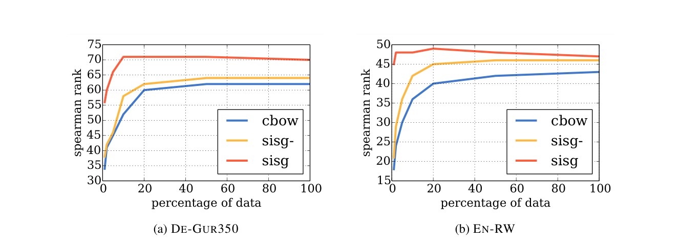
Figure 1: Influence of size of the training data on performance. We compute word vectors following the proposed model using datasets of increasing size. In this experiment, we train models on a fraction of the full Wikipedia dump.

图 1：训练数据规模对性能的影响。我们按提出的模型，在规模递增的数据集上计算词向量。本实验中，模型在完整维基百科转储的一个分数上训练。

As in the experiment presented in Sec. 5.1, not all words from the evaluation set are present in the Wikipedia data. Again, by default, we use a null vector for these words (sisg-) or compute a vector by summing the $n$-gram representations (sisg). The out-of-vocabulary rate is growing as the dataset shrinks, and therefore the performance of sisg- and cbow necessarily degrades. However, the proposed model (sisg) assigns non-trivial vectors to previously unseen words.

与第 5.1 节的实验一样，并非评估集中的所有词都出现在维基数据里。同样地，我们默认对这些词使用零向量（sisg-），或通过把 $n$-gram 表示相加来计算向量（sisg）。未登录词比例会随数据集缩小而上升，因此 sisg- 和 cbow 的性能必然会下降。不过，提出的模型（sisg）会给先前未见过的词赋予非平凡的向量。

First, we notice that for all datasets, and all sizes, the proposed approach (sisg) performs better than the baseline. However, the performance of the baseline cbow model gets better as more and more data is available. Our model, on the other hand, seems to quickly saturate and adding more data does not always lead to improved results.

首先，我们注意到，在所有数据集和所有规模上，提出的方法（sisg）都好于基线。不过，基线 cbow 模型的性能会随着数据增多而变好。我们的模型则似乎很快就趋于饱和，再增加数据并不总能带来更好的结果。

Second, and most importantly, we notice that the proposed approach provides very good word vectors even when using very small training datasets. For instance, on the German Gur350 dataset, our model (sisg) trained on $5\%$ of the data achieves better performance ($66$) than the cbow baseline trained on the full dataset ($62$). On the other hand, on the English RW dataset, using $1\%$ of the Wikipedia corpus we achieve a correlation coefficient of $45$ which is better than the performance of cbow trained on the full dataset ($43$). This has a very important practical implication: well performing word vectors can be computed on datasets of a restricted size and still work well on previously unseen words. In general, when using vectorial word representations in specific applications, it is recommended to retrain the model on textual data relevant for the application. However, this kind of relevant task-specific data is often very scarce and learning from a reduced amount of training data is a great advantage.

其次，也是最重要的一点，我们注意到，即使训练数据集非常小，提出的方法也能给出很好的词向量。例如，在德语 Gur350 数据集上，用 $5\%$ 的数据训练的模型（sisg）取得了比用全量数据训练的 cbow 基线（$62$）更好的性能（$66$）。另一方面，在英语 RW 数据集上，只用维基语料的 $1\%$，我们就得到了 $45$ 的相关系数，好于用全量数据训练的 cbow（$43$）。这有一个非常重要的实际含义：性能良好的词向量可以在规模受限的数据集上算出来，并且对先前未见过的词仍然管用。一般而言，在具体应用中使用向量词表示时，建议在与该应用相关的文本数据上重新训练模型。不过，这类相关的任务特定数据往往非常稀缺，能够从较少的训练数据中学习，是一个很大的优势。

5.5 Effect of the size of $n$-grams

5.5 $n$-gram 长度的影响

The proposed model relies on the use of character $n$-grams to represent words as vectors. As mentioned in Sec. 3.2, we decided to use $n$-grams ranging from $3$ to $6$ characters. This choice was arbitrary, motivated by the fact that $n$-grams of these lengths will cover a wide range of information. They would include short suffixes (corresponding to conjugations and declensions for instance) as well as longer roots. In this experiment, we empirically check for the influence of the range of $n$-grams that we use on performance. We report our results in Table 4 for English and German on word similarity and analogy datasets.

提出的模型依赖用字符 $n$-gram 把词表示成向量。如第 3.2 节所述，我们决定使用长度为 $3$ 到 $6$ 个字符的 $n$-gram。这一选择是任意的，动机是这些长度的 $n$-gram 能覆盖较广的信息：它们既包含短后缀（例如对应变位和变格），也包含较长的词根。本实验中，我们经验性地检查所用 $n$-gram 范围对性能的影响。我们在表 4 中报告英语和德语在词相似度和类比数据集上的结果。

(a) De-Gur350

	2	3	4	5	6
2	57	64	67	69	69
3		65	68	70	70
4			70	70	71
5				69	71
6					70

(b) De Semantic

	2	3	4	5	6
2	59	55	56	59	60
3		60	58	60	62
4			62	62	63
5				64	64
6					65

(c) De Syntactic

	2	3	4	5	6
2	45	50	53	54	55
3		51	55	55	56
4			54	56	56
5				56	56
6					54

(d) En-RW

	2	3	4	5	6
2	41	42	46	47	48
3		44	46	48	48
4			47	48	48
5				48	48
6					48

(e) En Semantic

	2	3	4	5	6
2	78	76	75	76	76
3		78	77	78	77
4			79	79	79
5				80	79
6					80

(f) En Syntactic

	2	3	4	5	6
2	70	71	73	74	73
3		72	74	75	74
4			74	75	75
5				74	74
6					72

Table 4: Study of the effect of sizes of $n$-grams considered on performance. We compute word vectors by using character $n$-grams with $n$ in $\{i, \ldots, j\}$ and report performance for various values of $i$ and $j$. We evaluate this effect on German and English, and represent out-of-vocabulary words using subword information.

(a) 德语 Gur350

	2	3	4	5	6
2	57	64	67	69	69
3		65	68	70	70
4			70	70	71
5				69	71
6					70

(b) 德语语义

	2	3	4	5	6
2	59	55	56	59	60
3		60	58	60	62
4			62	62	63
5				64	64
6					65

(c) 德语句法

	2	3	4	5	6
2	45	50	53	54	55
3		51	55	55	56
4			54	56	56
5				56	56
6					54

(d) 英语 RW

	2	3	4	5	6
2	41	42	46	47	48
3		44	46	48	48
4			47	48	48
5				48	48
6					48

(e) 英语语义

	2	3	4	5	6
2	78	76	75	76	76
3		78	77	78	77
4			79	79	79
5				80	79
6					80

(f) 英语句法

	2	3	4	5	6
2	70	71	73	74	73
3		72	74	75	74
4			74	75	75
5				74	74
6					72

表 4：所考虑 $n$-gram 长度对性能影响的研究。我们使用满足 $n$ 属于 $\{i, \ldots, j\}$ 的字符 $n$-gram 计算词向量，并报告不同 $i$、$j$ 取值下的性能。该影响在德语和英语上评估，未登录词用子词信息来表示。

We observe that for both English and German, our arbitrary choice of $3$-$6$ was a reasonable decision, as it provides satisfactory performance across languages. The optimal choice of length ranges depends on the considered task and language and should be tuned appropriately. However, due to the scarcity of test data, we did not implement any proper validation procedure to automatically select the best parameters. Nonetheless, taking a large range such as $3-6$ provides a reasonable amount of subword information.

我们观察到，对英语和德语而言，我们任意选定的 $3$-$6$ 是一个合理的决定，因为它在不同语言上都提供了令人满意的性能。最优的长度范围取决于所考虑的任务和语言，应当适当调整。不过，由于测试数据稀缺，我们没有实现任何自动选择最佳参数的正规验证程序。尽管如此，取 $3-6$ 这样较大的范围，已经能提供适量的子词信息。

This experiment also shows that it is important to include long $n$-grams, as columns corresponding to $n\leq 5$ and $n\leq 6$ work best. This is especially true for German, as many nouns are compounds made up from several units that can only be captured by longer character sequences. On analogy tasks, we observe that using larger $n$-grams helps for semantic analogies. However, results are always improved by taking $n\geq 3$ rather than $n\geq 2$, which shows that character $2$-grams are not informative for that task. As described in Sec. 3.2, before computing character $n$-grams, we prepend and append special positional characters to represent the beginning and end of word. Therefore, $2$-grams will not be enough to properly capture suffixes that correspond to conjugations or declensions, since they are composed of a single proper character and a positional one.

该实验还表明，纳入较长的 $n$-gram 很重要，因为对应 $n\leq 5$ 和 $n\leq 6$ 的各列效果最好。这对德语尤其如此，因为许多名词是由若干语素组成的复合词，只有较长的字符序列才能捕捉到。在类比任务上，我们观察到使用更长的 $n$-gram 对语义类比有帮助。不过，取 $n\geq 3$ 而不是 $n\geq 2$，结果总是更好，这说明字符二元组对该任务并没有信息量。如第 3.2 节所述，在计算字符 $n$-gram 之前，我们会在词的开头和结尾加上特殊的位置字符。因此，二元组不足以很好地捕捉对应变位或变格的后缀，因为它们由一个真正的字符和一个位置字符组成。

5.6 Language modeling

5.6 语言建模

In this section, we describe an evaluation of the word vectors obtained with our method on a language modeling task. We evaluate our language model on five languages (Cs, De, Es, Fr, Ru) using the datasets introduced by Botha and Blunsom (2014). Each dataset contains roughly one million training tokens, and we use the same preprocessing and data splits as Botha and Blunsom (2014).

本节描述把用我们的方法得到的词向量，放到语言建模任务上的一项评估。我们在五种语言（捷、德、西、法、俄）上评估语言模型，使用的是 Botha and Blunsom (2014) 提出的数据集。每个数据集大约有一百万个训练 token，我们采用与 Botha and Blunsom (2014) 相同的预处理和数据划分。

Our model is a recurrent neural network with $650$ LSTM units, regularized with dropout (with probability of $0.5$) and weight decay (regularization parameter of $10^{-5}$). We learn the parameters using the Adagrad algorithm with a learning rate of $0.1$, clipping the gradients which have a norm larger than $1.0$. We initialize the weight of the network in the range $[-0.05,0.05]$, and use a batch size of $20$. Two baselines are considered: we compare our approach to the log-bilinear language model of Botha and Blunsom (2014) and the character aware language model of Kim et al. (2016). We trained word vectors with character $n$-grams on the training set of the language modeling task and use them to initialize the lookup table of our language model. We report the test perplexity of our model without using pre-trained word vectors (LSTM), with word vectors pre-trained without subword information (sg) and with our vectors (sisg). The results are presented in Table 5.

我们的模型是一个有 $650$ 个 LSTM 单元的循环神经网络，用 dropout（概率为 $0.5$）和权值衰减（正则参数为 $10^{-5}$）做正则。参数用 Adagrad 算法学习，学习率为 $0.1$，并把范数大于 $1.0$ 的梯度裁剪掉。网络权重在 $[-0.05,0.05]$ 范围内初始化，批量大小为 $20$。我们考虑两个基线：Botha and Blunsom (2014) 的对数双线性语言模型，以及 Kim et al. (2016) 的字符感知语言模型。我们在语言建模任务的训练集上训练带字符 $n$-gram 的词向量，并用它们初始化语言模型的查找表。我们报告三种设置下的测试困惑度：不使用预训练词向量（LSTM）、使用不带子词信息的预训练词向量（sg），以及使用我们的向量（sisg）。结果见表 5。

	Cs	De	Es	Fr	Ru
Vocab. size	46k	37k	27k	25k	63k
CLBL	465	296	200	225	304
CANLM	371	239	165	184	261
LSTM	366	222	157	173	262
sg	339	216	150	162	237
sisg	312	206	145	159	206

Table 5: Test perplexity on the language modeling task, for 5 different languages. We compare to two state of the art approaches: CLBL refers to the work of Botha and Blunsom (2014) and CANLM refers to the work of Kim et al. (2016).

	捷	德	西	法	俄
词表大小	46k	37k	27k	25k	63k
CLBL	465	296	200	225	304
CANLM	371	239	165	184	261
LSTM	366	222	157	173	262
sg	339	216	150	162	237
sisg	312	206	145	159	206

表 5：五种语言上语言建模任务的测试困惑度。我们与两种当时最好的方法比较：CLBL 指 Botha and Blunsom (2014) 的工作，CANLM 指 Kim et al. (2016) 的工作。

	word	$n$-grams
	autofahrer	fahr	fahrer	auto
	freundeskreis	kreis	kreis>	<freun
De	grundwort	wort	wort>	grund
	sprachschule	schul	hschul	sprach
	tageslicht	licht	gesl	tages
	anarchy	chy	<anar	narchy
	monarchy	monarc	chy	<monar
	kindness	ness>	ness	kind
	politeness	polite	ness>	eness>
En	unlucky	<un	cky>	nlucky
	lifetime	life	<life	time
	starfish	fish	fish>	star
	submarine	marine	sub	marin
	transform	trans	<trans	form
	finirais	ais>	nir	fini
Fr	finissent	ent>	finiss	<finis
	finissions	ions>	finiss	sions>

Table 6: Illustration of most important character $n$-grams for selected words in three languages. For each word, we show the $n$-grams that, when removed, result in the most different representation.

	词	$n$-gram
	autofahrer	fahr	fahrer	auto
	freundeskreis	kreis	kreis>	<freun
德	grundwort	wort	wort>	grund
	sprachschule	schul	hschul	sprach
	tageslicht	licht	gesl	tages
	anarchy	chy	<anar	narchy
	monarchy	monarc	chy	<monar
	kindness	ness>	ness	kind
	politeness	polite	ness>	eness>
英	unlucky	<un	cky>	nlucky
	lifetime	life	<life	time
	starfish	fish	fish>	star
	submarine	marine	sub	marin
	transform	trans	<trans	form
	finirais	ais>	nir	fini
法	finissent	ent>	finiss	<finis
	finissions	ions>	finiss	sions>

表 6：三种语言中，若干词最重要的字符 $n$-gram 示例。对每个词，我们给出去掉之后会使表示变化最大的那些 $n$-gram。

We observe that initializing the lookup table of the language model with pre-trained word representations improves the test perplexity over the baseline LSTM. The most important observation is that using word representations trained with subword information outperforms the plain skipgram model. We observe that this improvement is most significant for morphologically rich Slavic languages such as Czech (8% reduction of perplexity over sg) and Russian (13% reduction). The improvement is less significant for Roman languages such as Spanish (3% reduction) or French (2% reduction). This shows the importance of subword information on the language modeling task and exhibits the usefulness of the vectors that we propose for morphologically rich languages.

我们观察到，用预训练词表示初始化语言模型的查找表，会比基线 LSTM 降低测试困惑度。最重要的观察是，用带子词信息训练的词表示，要好过普通的 skipgram 模型。这一改进在形态丰富的斯拉夫语上最为显著，例如捷克语（相对 sg，困惑度降低 8%）和俄语（降低 13%）。对西班牙语（降低 3%）或法语（降低 2%）这类罗曼语，改进则较小。这说明子词信息对语言建模任务很重要，也表明我们提出的向量对形态丰富的语言是有用的。

6 Qualitative analysis

6 定性分析

6.1 Nearest neighbors.

6.1 近邻。

We report sample qualitative results in Table 7. For selected words, we show nearest neighbors according to cosine similarity for vectors trained using the proposed approach and for the skipgram baseline. As expected, the nearest neighbors for complex, technical and infrequent words using our approach are better than the ones obtained using the baseline model.

我们在表 7 中报告若干定性结果。对选定的词，我们分别给出用提出方法和 skipgram 基线训练得到的向量按余弦相似度的近邻。正如所料，对复杂、专业且不常见的词，我们的方法给出的近邻要好于基线模型。

6.2 Character $n$-grams and morphemes

6.2 字符 $n$-gram 与语素

We want to qualitatively evaluate whether or not the most important $n$-grams in a word correspond to morphemes. To this end, we take a word vector that we construct as the sum of $n$-grams. As described in Sec. 3.2, each word $w$ is represented as the sum of its $n$-grams: $u_{w}=\sum_{g\in\mathcal{G}_{w}}z_{g}$. For each $n$-gram $g$, we propose to compute the restricted representation $u_{w\backslash g}$ obtained by omitting $g$:

我们希望定性地评估，一个词里最重要的 $n$-gram 是否对应于语素。为此，我们取由 $n$-gram 求和构成的词向量。如第 3.2 节所述，每个词 $w$ 表示成其 $n$-gram 的和：$u_{w}=\sum_{g\in\mathcal{G}_{w}}z_{g}$。对每个 $n$-gram $g$，我们计算去掉 $g$ 后得到的受限表示 $u_{w\backslash g}$：

$$u_{w\backslash g}=\sum_{g^{\prime}\in\mathcal{G}-\{g\}}z_{g^{\prime}}.$$

We then rank $n$-grams by increasing value of cosine between $u_{w}$ and $u_{w\backslash g}$. We show ranked $n$-grams for selected words in three languages in Table 6.

然后我们按 $u_{w}$ 与 $u_{w\backslash g}$ 之间余弦的升序给 $n$-gram 排序。三种语言中若干词的排序结果见表 6。

For German, which has a lot of compound nouns, we observe that the most important $n$-grams correspond to valid morphemes. Good examples include Autofahrer (car driver) whose most important $n$-grams are Auto (car) and Fahrer (driver). We also observe the separation of compound nouns into morphemes in English, with words such as lifetime or starfish. However, for English, we also observe that $n$-grams can correspond to affixes in words such as kindness or unlucky. Interestingly, for French we observe the inflections of verbs with endings such as ais>, ent> or ions>.

德语有很多复合名词，我们观察到最重要的 $n$-gram 对应于真正的语素。很好的例子是 Autofahrer（汽车司机），其最重要的 $n$-gram 是 Auto（汽车）和 Fahrer（司机）。在英语中，我们也观察到复合名词被拆成语素，例如 lifetime 或 starfish。不过对英语，我们还看到 $n$-gram 可以对应词缀，例如 kindness 或 unlucky。有意思的是，在法语中，我们观察到动词变位的词尾，例如 ais>、ent> 或 ions>。

6.3 Word similarity for OOV words

6.3 未登录词的词相似度

As described in Sec. 3.2, our model is capable of building word vectors for words that do not appear in the training set. For such words, we simply average the vector representation of its $n$-grams. In order to assess the quality of these representations, we analyze which of the $n$-grams match best for OOV words by selecting a few word pairs from the English RW similarity dataset. We select pairs such that one of the two words is not in the training vocabulary and is hence only represented by its $n$-grams. For each pair of words, we display the cosine similarity between each pair of $n$-grams that appear in the words. In order to simulate a setup with a larger number of OOV words, we use models trained on $1\%$ of the Wikipedia data as in Sec. 5.4. The results are presented in Fig. 2.

如第 3.2 节所述，我们的模型能够为未出现在训练集中的词构建词向量。对这些词，我们只要把它的 $n$-gram 向量表示取平均即可。为了评估这些表示的质量，我们从英语 RW 相似度数据集中选出若干词对，分析哪些 $n$-gram 对未登录词匹配得最好。我们选出这样一类词对：其中一词不在训练词表中，因而只由其 $n$-gram 来表示。对每一对词，我们展示出现在这两个词中的各对 $n$-gram 之间的余弦相似度。为了模拟未登录词更多的情形，我们使用如第 5.4 节那样在维基数据的 $1\%$ 上训练的模型。结果见图 2。

We observe interesting patterns, showing that subwords match correctly. Indeed, for the word chip, we clearly see that there are two groups of $n$-grams in microcircuit that match well. These roughly correspond to micro and circuit, and $n$-grams in between don’t match well. Another interesting example is the pair rarity and scarceness. Indeed, scarce roughly matches rarity while the suffix -ness matches -ity very well. Finally, the word preadolescent matches young well thanks to the -adolesc- subword. This shows that we build robust word representations where prefixes and suffixes can be ignored if the grammatical form is not found in the dictionary.

我们观察到一些有意思的模式，表明子词匹配是正确的。的确，对单词 chip，可以清楚地看到 microcircuit 里有两组 $n$-gram 匹配得很好。它们大致对应于 micro 和 circuit，而中间的 $n$-gram 则匹配不佳。另一个有意思的例子是 rarity 和 scarceness 这一对。的确，scarce 与 rarity 大致匹配，而后缀 -ness 与 -ity 匹配得非常好。最后，单词 preadolescent 凭借 -adolesc- 这一子词，与 young 匹配得很好。这表明我们构建的词表示相当稳健：如果词典里找不到相应的语法形式，前缀和后缀可以被忽略。

query	tiling	tech-rich	english-born	micromanaging	eateries	dendritic
sisg	tile	tech-dominated	british-born	micromanage	restaurants	dendrite
	flooring	tech-heavy	polish-born	micromanaged	eaterie	dendrites
sg	bookcases	technology-heavy	most-capped	defang	restaurants	epithelial
	built-ins	.ixic	ex-scotland	internalise	delis	p53

Table 7: Nearest neighbors of rare words using our representations and skipgram. These hand picked examples are for illustration.

查询	tiling	tech-rich	english-born	micromanaging	eateries	dendritic
sisg	tile	tech-dominated	british-born	micromanage	restaurants	dendrite
	flooring	tech-heavy	polish-born	micromanaged	eaterie	dendrites
sg	bookcases	technology-heavy	most-capped	defang	restaurants	epithelial
	built-ins	.ixic	ex-scotland	internalise	delis	p53

表 7：用我们的表示和 skipgram 得到的罕见词近邻。这些是手工挑选的示例，仅供说明。

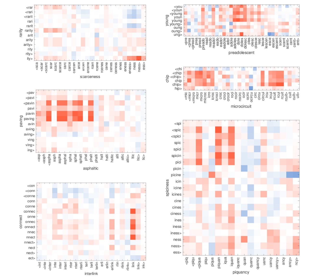
Figure 2: Illustration of the similarity between character $n$-grams in out-of-vocabulary words. For each pair, only one word is OOV, and is shown on the $x$ axis. Red indicates positive cosine, while blue negative.

图 2：未登录词中字符 $n$-gram 相似度的示意。对每一对词，只有一个是未登录词，并画在 $x$ 轴上。红色表示正的余弦，蓝色表示负的余弦。

7 Conclusion

7 结论

In this paper, we investigate a simple method to learn word representations by taking into account subword information. Our approach, which incorporates character $n$-grams into the skipgram model, is related to an idea that was introduced by Schütze (1993). Because of its simplicity, our model trains fast and does not require any preprocessing or supervision. We show that our model outperforms baselines that do not take into account subword information, as well as methods relying on morphological analysis. We will open source the implementation of our model, in order to facilitate comparison of future work on learning subword representations.

本文研究了一种把子词信息纳入考虑、学习词表示的简单方法。我们的做法是把字符 $n$-gram 引入 skipgram 模型，这与 Schütze (1993) 提出的想法相关。正因为简单，我们的模型训练很快，也不需要任何预处理或监督。我们表明，该模型既超过了不考虑子词信息的基线，也超过了依赖形态分析的方法。我们将开源模型实现，以便于后续关于学习子词表示的工作进行比较。

Acknowledgements

致谢

We thank Marco Baroni, Hinrich Schütze and the anonymous reviewers for their insightful comments.

我们感谢 Marco Baroni、Hinrich Schütze 以及匿名审稿人提出的富有见地的意见。

References

参考文献

[Alexandrescu and Kirchhoff (2006)] Andrei Alexandrescu and Katrin Kirchhoff. 2006. Factored neural language models. In Proc. NAACL .

[Ballesteros et al. (2015)] Miguel Ballesteros, Chris Dyer, and Noah A. Smith. 2015. Improved transition-based parsing by modeling characters instead of words with LSTMs. In Proc. EMNLP .

[Baroni and Lenci (2010)] Marco Baroni and Alessandro Lenci. 2010. Distributional memory: A general framework for corpus-based semantics. Computational Linguistics , 36(4):673–721.

[Berardi et al. (2015)] Giacomo Berardi, Andrea Esuli, and Diego Marcheggiani. 2015. Word embeddings go to Italy: a comparison of models and training datasets. Italian Information Retrieval Workshop .

[Bojanowski et al. (2015)] Piotr Bojanowski, Armand Joulin, and Tomáš Mikolov. 2015. Alternative structures for character-level RNNs. In Proc. ICLR .

[Botha and Blunsom (2014)] Jan A. Botha and Phil Blunsom. 2014. Compositional morphology for word representations and language modelling. In Proc. ICML .

[Chen et al. (2015)] Xinxiong Chen, Lei Xu, Zhiyuan Liu, Maosong Sun, and Huanbo Luan. 2015. Joint learning of character and word embeddings. In Proc. IJCAI .

[Chrupała (2014)] Grzegorz Chrupała. 2014. Normalizing tweets with edit scripts and recurrent neural embeddings. In Proc. ACL .

[Collobert and Weston (2008)] Ronan Collobert and Jason Weston. 2008. A unified architecture for natural language processing: Deep neural networks with multitask learning. In Proc. ICML .

[Cotterell and Schütze (2015)] Ryan Cotterell and Hinrich Schütze. 2015. Morphological word-embeddings. In Proc. NAACL .

[Cui et al. (2015)] Qing Cui, Bin Gao, Jiang Bian, Siyu Qiu, Hanjun Dai, and Tie-Yan Liu. 2015. KNET: A general framework for learning word embedding using morphological knowledge. ACM Transactions on Information Systems , 34(1):4:1–4:25.

[Deerwester et al. (1990)] Scott Deerwester, Susan T. Dumais, George W. Furnas, Thomas K. Landauer, and Richard Harshman. 1990. Indexing by latent semantic analysis. Journal of the American Society for Information Science , 41(6):391–407.

[dos Santos and Gatti (2014)] Cicero Nogueira dos Santos and Maira Gatti. 2014. Deep convolutional neural networks for sentiment analysis of short texts. In Proc. COLING .

[dos Santos and Zadrozny (2014)] Cicero Nogueira dos Santos and Bianca Zadrozny. 2014. Learning character-level representations for part-of-speech tagging. In Proc. ICML .

[Finkelstein et al. (2001)] Lev Finkelstein, Evgeniy Gabrilovich, Yossi Matias, Ehud Rivlin, Zach Solan, Gadi Wolfman, and Eytan Ruppin. 2001. Placing search in context: The concept revisited. In Proc. WWW .

[Graves (2013)] Alex Graves. 2013. Generating sequences with recurrent neural networks. arXiv preprint arXiv:1308.0850 .

[Gurevych (2005)] Iryna Gurevych. 2005. Using the structure of a conceptual network in computing semantic relatedness. In Proc. IJCNLP .

[Harris (1954)] Zellig S Harris. 1954. Distributional structure. Word , 10(2-3):146–162.

[Hassan and Mihalcea (2009)] Samer Hassan and Rada Mihalcea. 2009. Cross-lingual semantic relatedness using encyclopedic knowledge. In Proc. EMNLP .

[Joubarne and Inkpen (2011)] Colette Joubarne and Diana Inkpen. 2011. Comparison of semantic similarity for different languages using the google n-gram corpus and second-order co-occurrence measures. In Proc. Canadian Conference on Artificial Intelligence .

[Kim et al. (2016)] Yoon Kim, Yacine Jernite, David Sontag, and Alexander M Rush. 2016. Character-aware neural language models. In Proc. AAAI .

[Köper et al. (2015)] Maximilian Köper, Christian Scheible, and Sabine Schulte im Walde. 2015. Multilingual reliability and “semantic” structure of continuous word spaces. Proc. IWCS 2015 .

[Lazaridou et al. (2013)] Angeliki Lazaridou, Marco Marelli, Roberto Zamparelli, and Marco Baroni. 2013. Compositionally derived representations of morphologically complex words in distributional semantics. In Proc. ACL .

[Ling et al. (2015)] Wang Ling, Chris Dyer, Alan W. Black, Isabel Trancoso, Ramon Fermandez, Silvio Amir, Luis Marujo, and Tiago Luis. 2015. Finding function in form: Compositional character models for open vocabulary word representation. In Proc. EMNLP .

[Lund and Burgess (1996)] Kevin Lund and Curt Burgess. 1996. Producing high-dimensional semantic spaces from lexical co-occurrence. Behavior Research Methods, Instruments, & Computers , 28(2):203–208.

[Luong and Manning (2016)] Minh-Thang Luong and Christopher D. Manning. 2016. Achieving open vocabulary neural machine translation with hybrid word-character models. In Proc. ACL .

[Luong et al. (2013)] Thang Luong, Richard Socher, and Christopher D. Manning. 2013. Better word representations with recursive neural networks for morphology. In Proc. CoNLL .

[Mikolov et al. (2012)] Tomáš Mikolov, Ilya Sutskever, Anoop Deoras, Hai-Son Le, Stefan Kombrink, and Jan Černocký. 2012. Subword language modeling with neural networks. Technical report, Faculty of Information Technology, Brno University of Technology.

[Mikolov et al. (2013a)] Tomáš Mikolov, Kai Chen, Greg D. Corrado, and Jeffrey Dean. 2013a. Efficient estimation of word representations in vector space. arXiv preprint arXiv:1301.3781 .

[Mikolov et al. (2013b)] Tomáš Mikolov, Ilya Sutskever, Kai Chen, Greg S. Corrado, and Jeff Dean. 2013b. Distributed representations of words and phrases and their compositionality. In Adv. NIPS .

[Panchenko et al. (2016)] Alexander Panchenko, Dmitry Ustalov, Nikolay Arefyev, Denis Paperno, Natalia Konstantinova, Natalia Loukachevitch, and Chris Biemann. 2016. Human and machine judgements for russian semantic relatedness. In Proc. AIST .

[Qiu et al. (2014)] Siyu Qiu, Qing Cui, Jiang Bian, Bin Gao, and Tie-Yan Liu. 2014. Co-learning of word representations and morpheme representations. In Proc. COLING .

[Recht et al. (2011)] Benjamin Recht, Christopher Re, Stephen Wright, and Feng Niu. 2011. Hogwild: A lock-free approach to parallelizing stochastic gradient descent. In Adv. NIPS .

[Rumelhart et al. (1988)] David E. Rumelhart, Geoffrey E. Hinton, and Ronald J. Williams. 1988. Neurocomputing: Foundations of research. chapter Learning Representations by Back-propagating Errors, pages 696–699. MIT Press.

[Sak et al. (2010)] Haşim Sak, Murat Saraclar, and Tunga Gungör. 2010. Morphology-based and sub-word language modeling for turkish speech recognition. In Proc. ICASSP .

[Schütze (1992)] Hinrich Schütze. 1992. Dimensions of meaning. In Proc. IEEE Conference on Supercomputing .

[Schütze (1993)] Hinrich Schütze. 1993. Word space. In Adv. NIPS .

[Sennrich et al. (2016)] Rico Sennrich, Barry Haddow, and Alexandra Birch. 2016. Neural machine translation of rare words with subword units. In Proc. ACL .

[Shaoul and Westbury (2010)] Cyrus Shaoul and Chris Westbury. 2010. The Westbury lab Wikipedia corpus.

[Soricut and Och (2015)] Radu Soricut and Franz Och. 2015. Unsupervised morphology induction using word embeddings. In Proc. NAACL .

[Spearman (1904)] Charles Spearman. 1904. The proof and measurement of association between two things. The American Journal of Psychology , 15(1):72–101.

[Sperr et al. (2013)] Henning Sperr, Jan Niehues, and Alexander Waibel. 2013. Letter n-gram-based input encoding for continuous space language models. In Proc. of the Workshop on Continuous Vector Space Models and their Compositionality at ACL .

[Sutskever et al. (2011)] Ilya Sutskever, James Martens, and Geoffrey E Hinton. 2011. Generating text with recurrent neural networks. In Proc. ICML .

[Svoboda and Brychcin (2016)] Lukáš Svoboda and Tomáš Brychcin. 2016. New word analogy corpus for exploring embeddings of Czech words. In Proc. CICLING .

[Turney et al. (2010)] Peter D. Turney, Patrick Pantel, et al. 2010. From frequency to meaning: Vector space models of semantics. Journal of Artificial Intelligence Research , 37(1):141–188.

[Wieting et al. (2016)] John Wieting, Mohit Bansal, Kevin Gimpel, and Karen Livescu. 2016. CHARAGRAM: Embedding words and sentences via character n-grams. In Proc. EMNLP .

[Zesch and Gurevych (2006)] Torsten Zesch and Iryna Gurevych. 2006. Automatically creating datasets for measures of semantic relatedness. In Proc. Workshop on Linguistic Distances .

[Zhang et al. (2015)] Xiang Zhang, Junbo Zhao, and Yann LeCun. 2015. Character-level convolutional networks for text classification. In Adv. NIPS .