Fast R-CNN
Fast R-CNN
Ross Girshick Affiliation: Microsoft Research Email: rbg@microsoft.com
Abstract
摘要
This paper proposes a Fast Region-based Convolutional Network method (Fast R-CNN) for object detection. Fast R-CNN builds on previous work to efficiently classify object proposals using deep convolutional networks. Compared to previous work, Fast R-CNN employs several innovations to improve training and testing speed while also increasing detection accuracy. Fast R-CNN trains the very deep VGG16 network 9 faster than R-CNN, is 213 faster at test-time, and achieves a higher mAP on PASCAL VOC 2012. Compared to SPPnet, Fast R-CNN trains VGG16 3 faster, tests 10 faster, and is more accurate. Fast R-CNN is implemented in Python and C++ (using Caffe) and is available under the open-source MIT License at https://github.com/rbgirshick/fast-rcnn.
本文提出一种用于目标检测的快速区域卷积网络方法(Fast R-CNN)。它建立在已有工作之上,用深层卷积网络高效地为物体提议分类。与此前方法相比,Fast R-CNN 采用若干新设计,在提高检测精度的同时加快训练和测试。用很深的 VGG16 网络时,Fast R-CNN 的训练比 R-CNN 快 9 倍,测试快 213 倍,并且在 PASCAL VOC 2012 上得到更高的平均精度均值(mAP)。与 SPPnet 相比,它训练 VGG16 快 3 倍,测试快 10 倍,而且更准。Fast R-CNN 用 Python 和 C++(基于 Caffe)实现,以开源 MIT 许可证发布,地址为 https://github.com/rbgirshick/fast-rcnn。
1 Introduction
1 引言
Recently, deep ConvNets [14, 16] have significantly improved image classification [14] and object detection [9, 19] accuracy. Compared to image classification, object detection is a more challenging task that requires more complex methods to solve. Due to this complexity, current approaches (e.g., [9, 11, 19, 25]) train models in multi-stage pipelines that are slow and inelegant.
近年来,深层卷积网络 [14, 16] 显著提高了图像分类 [14] 和目标检测 [9, 19] 的精度。与图像分类相比,目标检测更难,也需要更复杂的方法。正因为这种复杂性,现有做法(例如 [9, 11, 19, 25])往往把模型训练做成多阶段流水线,既慢也不简洁。
Complexity arises because detection requires the accurate localization of objects, creating two primary challenges. First, numerous candidate object locations (often called “proposals”) must be processed. Second, these candidates provide only rough localization that must be refined to achieve precise localization. Solutions to these problems often compromise speed, accuracy, or simplicity.
复杂性来自检测必须把物体准确地定位出来,由此产生两个主要困难。第一,必须处理大量候选位置(常称为“提议”)。第二,这些候选往往只给出粗略定位,还需要再精细调整才能得到精确框。解决这两个问题的办法,常常要在速度、精度或简洁性上做取舍。
In this paper, we streamline the training process for state-of-the-art ConvNet-based object detectors [9, 11]. We propose a single-stage training algorithm that jointly learns to classify object proposals and refine their spatial locations.
本文把基于卷积网络的先进检测器 [9, 11] 的训练过程理顺。我们提出一种单阶段训练算法,同时学习给物体提议分类,并精细调整它们的空间位置。
The resulting method can train a very deep detection network (VGG16 [20]) 9 faster than R-CNN [9] and 3 faster than SPPnet [11]. At runtime, the detection network processes images in 0.3s (excluding object proposal time) while achieving top accuracy on PASCAL VOC 2012 [7] with a mAP of 66% (vs. 62% for R-CNN).[^1]
由此得到的方法可以把很深的检测网络(VGG16 [20])训得比 R-CNN [9] 快 9 倍,比 SPPnet [11] 快 3 倍。运行时,检测网络处理一张图只需 0.3 秒(不含生成物体提议的时间),并在 PASCAL VOC 2012 [7] 上取得当时最好的精度,mAP 为 66%(R-CNN 为 62%)。[^1]
1.1 R-CNN and SPPnet
1.1 R-CNN 与 SPPnet
The Region-based Convolutional Network method (R-CNN) [9] achieves excellent object detection accuracy by using a deep ConvNet to classify object proposals. R-CNN, however, has notable drawbacks:
基于区域的卷积网络方法(R-CNN)[9] 用深层卷积网络为物体提议分类,检测精度很高。不过 R-CNN 有几个明显缺点:
- Training is a multi-stage pipeline. R-CNN first fine-tunes a ConvNet on object proposals using log loss. Then, it fits SVMs to ConvNet features. These SVMs act as object detectors, replacing the softmax classifier learnt by fine-tuning. In the third training stage, bounding-box regressors are learned.
- 训练是多阶段流水线。 R-CNN 先在物体提议上用对数损失微调卷积网络,再在卷积特征上拟合 SVM。这些 SVM 充当检测器,替换微调时学到的 softmax 分类器。第三阶段再学习边界框回归器。
- Training is expensive in space and time. For SVM and bounding-box regressor training, features are extracted from each object proposal in each image and written to disk. With very deep networks, such as VGG16, this process takes 2.5 GPU-days for the 5k images of the VOC07 trainval set. These features require hundreds of gigabytes of storage.
- 训练在空间和时间上都昂贵。 为了训练 SVM 和边界框回归器,要从每张图的每个物体提议提取特征并写到磁盘。若使用 VGG16 这样很深的网络,仅 VOC07 trainval 的 5 千张图就要花 2.5 个 GPU-天。这些特征还需要数百 GB 的存储。
- Object detection is slow. At test-time, features are extracted from each object proposal in each test image. Detection with VGG16 takes 47s / image (on a GPU).
- 目标检测很慢。 测试时,要对每张测试图的每个物体提议提取特征。用 VGG16 检测一张图需要 47 秒(在 GPU 上)。
R-CNN is slow because it performs a ConvNet forward pass for each object proposal, without sharing computation. Spatial pyramid pooling networks (SPPnets) [11] were proposed to speed up R-CNN by sharing computation. The SPPnet method computes a convolutional feature map for the entire input image and then classifies each object proposal using a feature vector extracted from the shared feature map. Features are extracted for a proposal by max-pooling the portion of the feature map inside the proposal into a fixed-size output (e.g., ). Multiple output sizes are pooled and then concatenated as in spatial pyramid pooling [15]. SPPnet accelerates R-CNN by 10 to 100 at test time. Training time is also reduced by 3 due to faster proposal feature extraction.
R-CNN 之所以慢,是因为它对每个物体提议都单独做一次卷积网络前向传播,计算并不共享。空间金字塔池化网络(SPPnet)[11] 通过共享计算来加速 R-CNN。SPPnet 先为整张输入图计算一张卷积特征图,再从这张共享特征图上取出特征向量,为每个物体提议分类。取出特征的方式是:把提议框落在特征图上的那一块做最大池化,得到固定尺寸的输出(例如 )。多种输出尺寸会被池化后再拼接,就像空间金字塔池化 [15] 那样。测试时,SPPnet 把 R-CNN 加快 10 到 100 倍;由于提议特征提取变快,训练时间也缩短约 3 倍。
SPPnet also has notable drawbacks. Like R-CNN, training is a multi-stage pipeline that involves extracting features, fine-tuning a network with log loss, training SVMs, and finally fitting bounding-box regressors. Features are also written to disk. But unlike R-CNN, the fine-tuning algorithm proposed in [11] cannot update the convolutional layers that precede the spatial pyramid pooling. Unsurprisingly, this limitation (fixed convolutional layers) limits the accuracy of very deep networks.
SPPnet 同样有明显缺点。和 R-CNN 一样,训练仍是多阶段流水线:提取特征、用对数损失微调网络、训练 SVM,最后再拟合边界框回归器。特征同样要写到磁盘。但与 R-CNN 不同的是,[11] 提出的微调算法不能更新空间金字塔池化层之前的卷积层。这种限制(卷积层固定)会制约很深网络的精度,并不令人意外。
1.2 Contributions
1.2 贡献
We propose a new training algorithm that fixes the disadvantages of R-CNN and SPPnet, while improving on their speed and accuracy. We call this method Fast R-CNN because it’s comparatively fast to train and test. The Fast R-CNN method has several advantages:
我们提出一种新的训练算法,既补上 R-CNN 和 SPPnet 的不足,又在速度和精度上超过它们。我们把这种方法叫做 Fast R-CNN,因为它的训练和测试都比较快。Fast R-CNN 有几项优点:
- Higher detection quality (mAP) than R-CNN, SPPnet
- 检测质量(mAP)高于 R-CNN 和 SPPnet
- Training is single-stage, using a multi-task loss
- 训练是单阶段的,使用多任务损失
- Training can update all network layers
- 训练可以更新全部网络层
- No disk storage is required for feature caching
- 不必把特征缓存到磁盘
Fast R-CNN is written in Python and C++ (Caffe [13]) and is available under the open-source MIT License at https://github.com/rbgirshick/fast-rcnn.
Fast R-CNN 用 Python 和 C++(Caffe [13])写成,以开源 MIT 许可证发布,地址为 https://github.com/rbgirshick/fast-rcnn。
2 Fast R-CNN architecture and training
2 Fast R-CNN 的结构与训练
Fig. 1 illustrates the Fast R-CNN architecture. A Fast R-CNN network takes as input an entire image and a set of object proposals. The network first processes the whole image with several convolutional (conv) and max pooling layers to produce a conv feature map. Then, for each object proposal a region of interest (RoI) pooling layer extracts a fixed-length feature vector from the feature map. Each feature vector is fed into a sequence of fully connected (fc) layers that finally branch into two sibling output layers: one that produces softmax probability estimates over object classes plus a catch-all “background” class and another layer that outputs four real-valued numbers for each of the object classes. Each set of values encodes refined bounding-box positions for one of the classes.
图 1 给出了 Fast R-CNN 的结构。网络的输入是整张图像和一组物体提议。网络先用若干卷积(conv)层和最大池化层处理整张图,得到一张卷积特征图。然后,对每个物体提议,兴趣区域(RoI)池化层从特征图中取出一个固定长度的特征向量。每个特征向量再送入一系列全连接(fc)层,最后分成两个并列的输出层:一层给出 个物体类别再加一个“背景”类的 softmax 概率估计;另一层为这 个类别各输出 4 个实数。每组 4 个值编码的是该类 refinement 后的边界框位置。
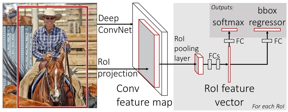
Figure 1: Fast R-CNN architecture. An input image and multiple regions of interest (RoIs) are input into a fully convolutional network. Each RoI is pooled into a fixed-size feature map and then mapped to a feature vector by fully connected layers (FCs). The network has two output vectors per RoI: softmax probabilities and per-class bounding-box regression offsets. The architecture is trained end-to-end with a multi-task loss.
图 1:Fast R-CNN 结构。输入图像和多个兴趣区域(RoI)被送入一个全卷积网络。每个 RoI 被池化成固定尺寸的特征图,再由全连接层(FC)映射成特征向量。每个 RoI 有两个输出向量:softmax 概率,以及按类别给出的边界框回归偏移。整个结构用多任务损失端到端训练。
2.1 The RoI pooling layer
2.1 RoI 池化层
The RoI pooling layer uses max pooling to convert the features inside any valid region of interest into a small feature map with a fixed spatial extent of (e.g., ), where and are layer hyper-parameters that are independent of any particular RoI. In this paper, an RoI is a rectangular window into a conv feature map. Each RoI is defined by a four-tuple that specifies its top-left corner and its height and width .
RoI 池化层用最大池化,把任意有效兴趣区域内的特征转换成空间尺寸固定为 (例如 )的小特征图,其中 和 是与具体 RoI 无关的层超参数。本文中,RoI 是卷积特征图上的一个矩形窗口。每个 RoI 由四元组 定义,给出左上角 以及高和宽 。
RoI max pooling works by dividing the RoI window into an grid of sub-windows of approximate size and then max-pooling the values in each sub-window into the corresponding output grid cell. Pooling is applied independently to each feature map channel, as in standard max pooling. The RoI layer is simply the special-case of the spatial pyramid pooling layer used in SPPnets [11] in which there is only one pyramid level. We use the pooling sub-window calculation given in [11].
RoI 最大池化的做法是:把 的 RoI 窗口划分成 的子窗口网格,每个子窗口大小约为 ,再把每个子窗口里的值最大池化到对应的输出网格单元。池化对每个特征图通道独立进行,和标准最大池化一样。RoI 层其实就是 SPPnet [11] 所用空间金字塔池化层在只有一层金字塔时的特例。子窗口的划分计算我们采用 [11] 中的方法。
2.2 Initializing from pre-trained networks
2.2 从预训练网络初始化
We experiment with three pre-trained ImageNet [4] networks, each with five max pooling layers and between five and thirteen conv layers (see Section 4.1 for network details). When a pre-trained network initializes a Fast R-CNN network, it undergoes three transformations.
我们实验了三个在 ImageNet [4] 上预训练的网络,它们都有五层最大池化,卷积层数从五层到十三层不等(网络细节见第 4.1 节)。用预训练网络初始化 Fast R-CNN 时,要做三处改动。
First, the last max pooling layer is replaced by a RoI pooling layer that is configured by setting and to be compatible with the net’s first fully connected layer (e.g., for VGG16).
第一,把最后一层最大池化换成 RoI 池化层,并把 和 设成与网络第一个全连接层兼容(例如对 VGG16 取 )。
Second, the network’s last fully connected layer and softmax (which were trained for 1000-way ImageNet classification) are replaced with the two sibling layers described earlier (a fully connected layer and softmax over categories and category-specific bounding-box regressors).
第二,把原先为 ImageNet 一千类分类训练的最后一个全连接层和 softmax,换成前面描述的两个并列层(一个对 类做全连接加 softmax,以及按类别的边界框回归器)。
Third, the network is modified to take two data inputs: a list of images and a list of RoIs in those images.
第三,把网络改成接受两个数据输入:一组图像,以及这些图像中的一组 RoI。
2.3 Fine-tuning for detection
2.3 面向检测的微调
Training all network weights with back-propagation is an important capability of Fast R-CNN. First, let’s elucidate why SPPnet is unable to update weights below the spatial pyramid pooling layer.
用反向传播训练全部网络权重,是 Fast R-CNN 的一项重要能力。我们先说明,为什么 SPPnet 无法更新空间金字塔池化层以下的权重。
The root cause is that back-propagation through the SPP layer is highly inefficient when each training sample (i.e. RoI) comes from a different image, which is exactly how R-CNN and SPPnet networks are trained. The inefficiency stems from the fact that each RoI may have a very large receptive field, often spanning the entire input image. Since the forward pass must process the entire receptive field, the training inputs are large (often the entire image).
根本原因是:当每个训练样本(即每个 RoI)来自不同图像时——而这正是 R-CNN 和 SPPnet 的训练方式——通过 SPP 层做反向传播会非常低效。低效是因为每个 RoI 的感受野可能非常大,常常覆盖整张输入图。前向传播必须处理整个感受野,于是训练输入往往就是整张图,体积很大。
We propose a more efficient training method that takes advantage of feature sharing during training. In Fast R-CNN training, stochastic gradient descent (SGD) mini-batches are sampled hierarchically, first by sampling images and then by sampling RoIs from each image. Critically, RoIs from the same image share computation and memory in the forward and backward passes. Making small decreases mini-batch computation. For example, when using and , the proposed training scheme is roughly 64 faster than sampling one RoI from different images (i.e., the R-CNN and SPPnet strategy).
我们提出一种更高效的训练方法,在训练时利用特征共享。Fast R-CNN 的随机梯度下降(SGD)小批量是分层采样的:先采样 张图,再从每张图采样 个 RoI。关键在于,同一张图上的 RoI 在前向和反向传播中共享计算和内存。把 取得小,可以减少小批量的计算量。例如,当 、 时,这种训练方案大约比从 128 张不同图各采一个 RoI(也就是 R-CNN 和 SPPnet 的策略)快 64 倍。
One concern over this strategy is it may cause slow training convergence because RoIs from the same image are correlated. This concern does not appear to be a practical issue and we achieve good results with and using fewer SGD iterations than R-CNN.
一种担心是:同一张图上的 RoI 相互相关,可能导致训练收敛变慢。这个问题在实践中似乎并不严重;我们用 、,以比 R-CNN 更少的 SGD 迭代就取得了好结果。
In addition to hierarchical sampling, Fast R-CNN uses a streamlined training process with one fine-tuning stage that jointly optimizes a softmax classifier and bounding-box regressors, rather than training a softmax classifier, SVMs, and regressors in three separate stages [9, 11]. The components of this procedure (the loss, mini-batch sampling strategy, back-propagation through RoI pooling layers, and SGD hyper-parameters) are described below.
除了分层采样,Fast R-CNN 还把训练收成一个微调阶段,同时优化 softmax 分类器和边界框回归器,而不是像 [9, 11] 那样分三个阶段分别训练 softmax 分类器、SVM 和回归器。下面说明这一过程的各个部分(损失、小批量采样策略、通过 RoI 池化层的反向传播,以及 SGD 超参数)。
Multi-task loss.
A Fast R-CNN network has two sibling output layers. The first outputs a discrete probability distribution (per RoI), , over categories. As usual, is computed by a softmax over the outputs of a fully connected layer. The second sibling layer outputs bounding-box regression offsets, , for each of the object classes, indexed by . We use the parameterization for given in [9], in which specifies a scale-invariant translation and log-space height/width shift relative to an object proposal.
多任务损失。
Fast R-CNN 网络有两个并列的输出层。第一个输出每个 RoI 在 个类别上的离散概率分布 。和通常做法一样, 是对全连接层的 个输出做 softmax 得到的。第二个并列层为 个物体类别各输出一组边界框回归偏移 ,用 索引类别。 的参数化采用 [9] 中的定义,表示相对物体提议的尺度不变平移,以及对数空间中的高宽平移。
Each training RoI is labeled with a ground-truth class and a ground-truth bounding-box regression target . We use a multi-task loss on each labeled RoI to jointly train for classification and bounding-box regression:
每个训练 RoI 都标有真实类别 和真实边界框回归目标 。我们在每个已标注 RoI 上使用多任务损失 ,联合训练分类和边界框回归:
in which is log loss for true class .
其中 是真实类别 上的对数损失。
The second task loss, , is defined over a tuple of true bounding-box regression targets for class , , and a predicted tuple , again for class . The Iverson bracket indicator function evaluates to 1 when and 0 otherwise. By convention the catch-all background class is labeled . For background RoIs there is no notion of a ground-truth bounding box and hence is ignored. For bounding-box regression, we use the loss
第二个任务损失 定义在类别 的真实边界框回归目标 与预测元组 上,二者都对应于类别 。艾弗森括号指示函数 在 时取 1,否则取 0。按惯例,背景类标记为 。对背景 RoI 不存在真实边界框,因此 被忽略。边界框回归使用的损失为
in which
其中
$$\textrm{smooth}{L{1}}(x)=\begin{cases}0.5x^{2}&\text{if }|x|<1\
|x|-0.5&\text{otherwise},\end{cases} \tag{3}$$
is a robust loss that is less sensitive to outliers than the loss used in R-CNN and SPPnet. When the regression targets are unbounded, training with loss can require careful tuning of learning rates in order to prevent exploding gradients. Eq. 3 eliminates this sensitivity.
是一种稳健的 损失,对离群点不如 R-CNN 和 SPPnet 所用的 损失敏感。当回归目标无界时,用 损失训练可能需要仔细调节学习率,以免梯度爆炸。式 3 消除了这种敏感性。
The hyper-parameter in Eq. 1 controls the balance between the two task losses. We normalize the ground-truth regression targets to have zero mean and unit variance. All experiments use .
式 1 中的超参数 控制两个任务损失的平衡。我们把真实回归目标 归一化到零均值、单位方差。全部实验都取 。
We note that [6] uses a related loss to train a class-agnostic object proposal network. Different from our approach, [6] advocates for a two-network system that separates localization and classification. OverFeat [19], R-CNN [9], and SPPnet [11] also train classifiers and bounding-box localizers, however these methods use stage-wise training, which we show is suboptimal for Fast R-CNN (Section 5.1).
需要说明的是,[6] 用一种相关的损失来训练与类别无关的物体提议网络。与我们不同,[6] 主张用两套网络分别做定位和分类。OverFeat [19]、R-CNN [9] 和 SPPnet [11] 也训练分类器和边界框定位器,但这些方法采用分阶段训练;我们在第 5.1 节表明,这对 Fast R-CNN 并非最优。
Mini-batch sampling.
During fine-tuning, each SGD mini-batch is constructed from images, chosen uniformly at random (as is common practice, we actually iterate over permutations of the dataset). We use mini-batches of size , sampling RoIs from each image. As in [9], we take 25% of the RoIs from object proposals that have intersection over union (IoU) overlap with a ground-truth bounding box of at least . These RoIs comprise the examples labeled with a foreground object class, i.e. . The remaining RoIs are sampled from object proposals that have a maximum IoU with ground truth in the interval , following [11]. These are the background examples and are labeled with . The lower threshold of appears to act as a heuristic for hard example mining [8]. During training, images are horizontally flipped with probability . No other data augmentation is used.
小批量采样。
微调时,每个 SGD 小批量由 张图构成,这些图均匀随机选取(和常见做法一样,我们实际是按数据集的随机排列迭代)。小批量大小为 ,从每张图采样 64 个 RoI。与 [9] 一样,我们把 25% 的 RoI 取自与某个真实框的交并比(IoU)至少为 的物体提议。这些 RoI 作为前景物体类别的样本,即 。其余 RoI 从与真实框的最大 IoU 落在区间 内的物体提议中采样,做法遵循 [11]。这些是背景样本,标记为 。下限 看起来像一种难例挖掘的启发式规则 [8]。训练时,图像以 的概率做水平翻转。不再使用其他数据增广。
Back-propagation through RoI pooling layers.
Back-propagation routes derivatives through the RoI pooling layer. For clarity, we assume only one image per mini-batch (), though the extension to is straightforward because the forward pass treats all images independently.
通过 RoI 池化层的反向传播。
反向传播要把导数路由过 RoI 池化层。为清楚起见,我们先假设每个小批量只有一张图();由于前向传播对所有图像是独立处理的,推广到 很直接。
Let be the -th activation input into the RoI pooling layer and let be the layer’s -th output from the -th RoI. The RoI pooling layer computes , in which . is the index set of inputs in the sub-window over which the output unit max pools. A single may be assigned to several different outputs .
设 是送入 RoI 池化层的第 个激活输入,设 是该层来自第 个 RoI 的第 个输出。RoI 池化层计算 ,其中 。 是输出单元 做最大池化时所覆盖子窗口中的输入下标集合。同一个 可能被赋给若干不同的输出 。
The RoI pooling layer’s backwards function computes partial derivative of the loss function with respect to each input variable by following the argmax switches:
RoI 池化层的反向函数按照 argmax 开关,计算损失函数对每个输入变量 的偏导数:
In words, for each mini-batch RoI and for each pooling output unit , the partial derivative is accumulated if is the argmax selected for by max pooling. In back-propagation, the partial derivatives are already computed by the backwards function of the layer on top of the RoI pooling layer.
用话说:对小批量中的每个 RoI 和每个池化输出单元 ,如果 是最大池化为 选出的 argmax,就把偏导数 累加进去。在反向传播中,偏导数 已经由 RoI 池化层之上那一层的反向函数算好了。
SGD hyper-parameters.
The fully connected layers used for softmax classification and bounding-box regression are initialized from zero-mean Gaussian distributions with standard deviations and , respectively. Biases are initialized to . All layers use a per-layer learning rate of 1 for weights and 2 for biases and a global learning rate of . When training on VOC07 or VOC12 trainval we run SGD for 30k mini-batch iterations, and then lower the learning rate to and train for another 10k iterations. When we train on larger datasets, we run SGD for more iterations, as described later. A momentum of and parameter decay of (on weights and biases) are used.
SGD 超参数。
用于 softmax 分类和边界框回归的全连接层,分别用标准差为 和 的零均值高斯分布初始化。偏置初始化为 。所有层对权重使用 1 倍的逐层学习率,对偏置使用 2 倍,全局学习率为 。在 VOC07 或 VOC12 的 trainval 上训练时,我们先跑 3 万次小批量迭代,再把学习率降到 ,继续训练 1 万次。在更大的数据集上训练时,迭代次数会更多,后文再说明。动量取 ,参数衰减取 (作用于权重和偏置)。
2.4 Scale invariance
2.4 尺度不变性
We explore two ways of achieving scale invariant object detection: (1) via “brute force” learning and (2) by using image pyramids. These strategies follow the two approaches in [11]. In the brute-force approach, each image is processed at a pre-defined pixel size during both training and testing. The network must directly learn scale-invariant object detection from the training data.
我们探索了两种实现尺度不变目标检测的途径:(1)“蛮力”学习;(2)使用图像金字塔。这两种策略对应于 [11] 中的两种做法。在蛮力方法里,训练和测试时每张图都处理到一个预先设定的像素尺寸。网络必须直接从训练数据中学会尺度不变的目标检测。
The multi-scale approach, in contrast, provides approximate scale-invariance to the network through an image pyramid. At test-time, the image pyramid is used to approximately scale-normalize each object proposal. During multi-scale training, we randomly sample a pyramid scale each time an image is sampled, following [11], as a form of data augmentation. We experiment with multi-scale training for smaller networks only, due to GPU memory limits.
多尺度方法则相反,通过图像金字塔给网络提供近似的尺度不变性。测试时,用图像金字塔把每个物体提议近似地尺度归一化。多尺度训练时,每当采到一张图,我们就随机采样一个金字塔尺度,做法遵循 [11],这也可以看成一种数据增广。受 GPU 显存限制,我们只在较小的网络上实验了多尺度训练。
3 Fast R-CNN detection
3 Fast R-CNN 检测
Once a Fast R-CNN network is fine-tuned, detection amounts to little more than running a forward pass (assuming object proposals are pre-computed). The network takes as input an image (or an image pyramid, encoded as a list of images) and a list of object proposals to score. At test-time, is typically around , although we will consider cases in which it is larger ( k). When using an image pyramid, each RoI is assigned to the scale such that the scaled RoI is closest to pixels in area [11].
Fast R-CNN 网络微调完成后,检测基本上就是做一次前向传播(假定物体提议已经预先算好)。网络的输入是一张图(或编码成图像列表的图像金字塔),以及要打分的 个物体提议。测试时 通常约为 2000,不过我们也会考虑更大的情形(约 4.5 万)。若使用图像金字塔,每个 RoI 会被分配到缩放后面积最接近 像素的那个尺度 [11]。
For each test RoI , the forward pass outputs a class posterior probability distribution and a set of predicted bounding-box offsets relative to (each of the classes gets its own refined bounding-box prediction). We assign a detection confidence to for each object class using the estimated probability . We then perform non-maximum suppression independently for each class using the algorithm and settings from R-CNN [9].
对每个测试 RoI ,前向传播输出类别后验概率分布 ,以及相对 的一组预测边界框偏移( 个类别各自得到 精细调整后的边界框预测)。我们对每个物体类别 ,用估计概率 作为 的检测置信度。然后对每个类别独立做非极大值抑制,算法和设定与 R-CNN [9] 相同。
3.1 Truncated SVD for faster detection
3.1 用截断 SVD 加快检测
For whole-image classification, the time spent computing the fully connected layers is small compared to the conv layers. On the contrary, for detection the number of RoIs to process is large and nearly half of the forward pass time is spent computing the fully connected layers (see Fig. 2). Large fully connected layers are easily accelerated by compressing them with truncated SVD [5, 23].
对整图分类来说,全连接层所占时间相对卷积层很小。检测则相反:要处理的 RoI 数量很多,前向传播近一半时间花在计算全连接层上(见图 2)。大型全连接层很容易用截断 SVD 压缩来加速 [5, 23]。
In this technique, a layer parameterized by the weight matrix is approximately factorized as
在这种技术里,由 权重矩阵 参数化的一层被近似分解为
using SVD. In this factorization, is a matrix comprising the first left-singular vectors of , is a diagonal matrix containing the top singular values of , and is matrix comprising the first right-singular vectors of . Truncated SVD reduces the parameter count from to , which can be significant if is much smaller than . To compress a network, the single fully connected layer corresponding to is replaced by two fully connected layers, without a non-linearity between them. The first of these layers uses the weight matrix (and no biases) and the second uses (with the original biases associated with ). This simple compression method gives good speedups when the number of RoIs is large.
分解通过 SVD 完成。其中 是 矩阵,由 的前 个左奇异向量组成; 是包含 最大的 个奇异值的 对角矩阵; 是由 的前 个右奇异向量组成的 矩阵。截断 SVD 把参数量从 降到 ,当 远小于 时,压缩可以相当可观。为了压缩网络,对应于 的那一个全连接层被换成两个中间没有非线性的全连接层。第一层使用权重矩阵 (没有偏置),第二层使用 (沿用原先与 相连的偏置)。当 RoI 数量很大时,这种简单的压缩方法能带来可观的加速。
4 Main results
4 主要结果
| method | train set | aero | bike | bird | boat | bottle | bus | car | cat | chair | cow | table | dog | horse | mbike | persn | plant | sheep | sofa | train | tv | mAP |
|---|---|---|---|---|---|---|---|---|---|---|---|---|---|---|---|---|---|---|---|---|---|---|
| SPPnet BB [11]† | 07 diff | 73.9 | 72.3 | 62.5 | 51.5 | 44.4 | 74.4 | 73.0 | 74.4 | 42.3 | 73.6 | 57.7 | 70.3 | 74.6 | 74.3 | 54.2 | 34.0 | 56.4 | 56.4 | 67.9 | 73.5 | 63.1 |
| R-CNN BB [10] | 07 | 73.4 | 77.0 | 63.4 | 45.4 | 44.6 | 75.1 | 78.1 | 79.8 | 40.5 | 73.7 | 62.2 | 79.4 | 78.1 | 73.1 | 64.2 | 35.6 | 66.8 | 67.2 | 70.4 | 71.1 | 66.0 |
| FRCN [ours] | 07 | 74.5 | 78.3 | 69.2 | 53.2 | 36.6 | 77.3 | 78.2 | 82.0 | 40.7 | 72.7 | 67.9 | 79.6 | 79.2 | 73.0 | 69.0 | 30.1 | 65.4 | 70.2 | 75.8 | 65.8 | 66.9 |
| FRCN [ours] | 07 diff | 74.6 | 79.0 | 68.6 | 57.0 | 39.3 | 79.5 | 78.6 | 81.9 | 48.0 | 74.0 | 67.4 | 80.5 | 80.7 | 74.1 | 69.6 | 31.8 | 67.1 | 68.4 | 75.3 | 65.5 | 68.1 |
| FRCN [ours] | 07+12 | 77.0 | 78.1 | 69.3 | 59.4 | 38.3 | 81.6 | 78.6 | 86.7 | 42.8 | 78.8 | 68.9 | 84.7 | 82.0 | 76.6 | 69.9 | 31.8 | 70.1 | 74.8 | 80.4 | 70.4 | 70.0 |
Table 1: VOC 2007 test detection average precision (%). All methods use VGG16. Training set key: 07: VOC07 trainval, 07 diff: 07 without “difficult” examples, 07+12: union of 07 and VOC12 trainval. †SPPnet results were prepared by the authors of [11].
| 方法 | 训练集 | aero | bike | bird | boat | bottle | bus | car | cat | chair | cow | table | dog | horse | mbike | persn | plant | sheep | sofa | train | tv | mAP |
|---|---|---|---|---|---|---|---|---|---|---|---|---|---|---|---|---|---|---|---|---|---|---|
| SPPnet BB [11]† | 07 diff | 73.9 | 72.3 | 62.5 | 51.5 | 44.4 | 74.4 | 73.0 | 74.4 | 42.3 | 73.6 | 57.7 | 70.3 | 74.6 | 74.3 | 54.2 | 34.0 | 56.4 | 56.4 | 67.9 | 73.5 | 63.1 |
| R-CNN BB [10] | 07 | 73.4 | 77.0 | 63.4 | 45.4 | 44.6 | 75.1 | 78.1 | 79.8 | 40.5 | 73.7 | 62.2 | 79.4 | 78.1 | 73.1 | 64.2 | 35.6 | 66.8 | 67.2 | 70.4 | 71.1 | 66.0 |
| FRCN [本文] | 07 | 74.5 | 78.3 | 69.2 | 53.2 | 36.6 | 77.3 | 78.2 | 82.0 | 40.7 | 72.7 | 67.9 | 79.6 | 79.2 | 73.0 | 69.0 | 30.1 | 65.4 | 70.2 | 75.8 | 65.8 | 66.9 |
| FRCN [本文] | 07 diff | 74.6 | 79.0 | 68.6 | 57.0 | 39.3 | 79.5 | 78.6 | 81.9 | 48.0 | 74.0 | 67.4 | 80.5 | 80.7 | 74.1 | 69.6 | 31.8 | 67.1 | 68.4 | 75.3 | 65.5 | 68.1 |
| FRCN [本文] | 07+12 | 77.0 | 78.1 | 69.3 | 59.4 | 38.3 | 81.6 | 78.6 | 86.7 | 42.8 | 78.8 | 68.9 | 84.7 | 82.0 | 76.6 | 69.9 | 31.8 | 70.1 | 74.8 | 80.4 | 70.4 | 70.0 |
表 1:VOC 2007 测试集检测平均精度(%)。所有方法都使用 VGG16。训练集代号:07:VOC07 trainval,07 diff:去掉“困难”样本后的 07,07+12:07 与 VOC12 trainval 的并集。†SPPnet 结果由 [11] 的作者提供。
| method | train set | aero | bike | bird | boat | bottle | bus | car | cat | chair | cow | table | dog | horse | mbike | persn | plant | sheep | sofa | train | tv | mAP |
|---|---|---|---|---|---|---|---|---|---|---|---|---|---|---|---|---|---|---|---|---|---|---|
| BabyLearning | Prop. | 77.7 | 73.8 | 62.3 | 48.8 | 45.4 | 67.3 | 67.0 | 80.3 | 41.3 | 70.8 | 49.7 | 79.5 | 74.7 | 78.6 | 64.5 | 36.0 | 69.9 | 55.7 | 70.4 | 61.7 | 63.8 |
| R-CNN BB [10] | 12 | 79.3 | 72.4 | 63.1 | 44.0 | 44.4 | 64.6 | 66.3 | 84.9 | 38.8 | 67.3 | 48.4 | 82.3 | 75.0 | 76.7 | 65.7 | 35.8 | 66.2 | 54.8 | 69.1 | 58.8 | 62.9 |
| SegDeepM | 12+seg | 82.3 | 75.2 | 67.1 | 50.7 | 49.8 | 71.1 | 69.6 | 88.2 | 42.5 | 71.2 | 50.0 | 85.7 | 76.6 | 81.8 | 69.3 | 41.5 | 71.9 | 62.2 | 73.2 | 64.6 | 67.2 |
| FRCN [ours] | 12 | 80.1 | 74.4 | 67.7 | 49.4 | 41.4 | 74.2 | 68.8 | 87.8 | 41.9 | 70.1 | 50.2 | 86.1 | 77.3 | 81.1 | 70.4 | 33.3 | 67.0 | 63.3 | 77.2 | 60.0 | 66.1 |
| FRCN [ours] | 07++12 | 82.0 | 77.8 | 71.6 | 55.3 | 42.4 | 77.3 | 71.7 | 89.3 | 44.5 | 72.1 | 53.7 | 87.7 | 80.0 | 82.5 | 72.7 | 36.6 | 68.7 | 65.4 | 81.1 | 62.7 | 68.8 |
Table 2: VOC 2010 test detection average precision (%). BabyLearning uses a network based on [17]. All other methods use VGG16. Training set key: 12: VOC12 trainval, Prop.: proprietary dataset, 12+seg: 12 with segmentation annotations, 07++12: union of VOC07 trainval, VOC07 test, and VOC12 trainval.
| 方法 | 训练集 | aero | bike | bird | boat | bottle | bus | car | cat | chair | cow | table | dog | horse | mbike | persn | plant | sheep | sofa | train | tv | mAP |
|---|---|---|---|---|---|---|---|---|---|---|---|---|---|---|---|---|---|---|---|---|---|---|
| BabyLearning | Prop. | 77.7 | 73.8 | 62.3 | 48.8 | 45.4 | 67.3 | 67.0 | 80.3 | 41.3 | 70.8 | 49.7 | 79.5 | 74.7 | 78.6 | 64.5 | 36.0 | 69.9 | 55.7 | 70.4 | 61.7 | 63.8 |
| R-CNN BB [10] | 12 | 79.3 | 72.4 | 63.1 | 44.0 | 44.4 | 64.6 | 66.3 | 84.9 | 38.8 | 67.3 | 48.4 | 82.3 | 75.0 | 76.7 | 65.7 | 35.8 | 66.2 | 54.8 | 69.1 | 58.8 | 62.9 |
| SegDeepM | 12+seg | 82.3 | 75.2 | 67.1 | 50.7 | 49.8 | 71.1 | 69.6 | 88.2 | 42.5 | 71.2 | 50.0 | 85.7 | 76.6 | 81.8 | 69.3 | 41.5 | 71.9 | 62.2 | 73.2 | 64.6 | 67.2 |
| FRCN [本文] | 12 | 80.1 | 74.4 | 67.7 | 49.4 | 41.4 | 74.2 | 68.8 | 87.8 | 41.9 | 70.1 | 50.2 | 86.1 | 77.3 | 81.1 | 70.4 | 33.3 | 67.0 | 63.3 | 77.2 | 60.0 | 66.1 |
| FRCN [本文] | 07++12 | 82.0 | 77.8 | 71.6 | 55.3 | 42.4 | 77.3 | 71.7 | 89.3 | 44.5 | 72.1 | 53.7 | 87.7 | 80.0 | 82.5 | 72.7 | 36.6 | 68.7 | 65.4 | 81.1 | 62.7 | 68.8 |
表 2:VOC 2010 测试集检测平均精度(%)。BabyLearning 使用基于 [17] 的网络。其余方法都使用 VGG16。训练集代号:12:VOC12 trainval,Prop.:专有数据集,12+seg:带分割标注的 12,07++12:VOC07 trainval、VOC07 test 与 VOC12 trainval 的并集。
| method | train set | aero | bike | bird | boat | bottle | bus | car | cat | chair | cow | table | dog | horse | mbike | persn | plant | sheep | sofa | train | tv | mAP |
|---|---|---|---|---|---|---|---|---|---|---|---|---|---|---|---|---|---|---|---|---|---|---|
| BabyLearning | Prop. | 78.0 | 74.2 | 61.3 | 45.7 | 42.7 | 68.2 | 66.8 | 80.2 | 40.6 | 70.0 | 49.8 | 79.0 | 74.5 | 77.9 | 64.0 | 35.3 | 67.9 | 55.7 | 68.7 | 62.6 | 63.2 |
| NUS_NIN_c2000 | Unk. | 80.2 | 73.8 | 61.9 | 43.7 | 43.0 | 70.3 | 67.6 | 80.7 | 41.9 | 69.7 | 51.7 | 78.2 | 75.2 | 76.9 | 65.1 | 38.6 | 68.3 | 58.0 | 68.7 | 63.3 | 63.8 |
| R-CNN BB [10] | 12 | 79.6 | 72.7 | 61.9 | 41.2 | 41.9 | 65.9 | 66.4 | 84.6 | 38.5 | 67.2 | 46.7 | 82.0 | 74.8 | 76.0 | 65.2 | 35.6 | 65.4 | 54.2 | 67.4 | 60.3 | 62.4 |
| FRCN [ours] | 12 | 80.3 | 74.7 | 66.9 | 46.9 | 37.7 | 73.9 | 68.6 | 87.7 | 41.7 | 71.1 | 51.1 | 86.0 | 77.8 | 79.8 | 69.8 | 32.1 | 65.5 | 63.8 | 76.4 | 61.7 | 65.7 |
| FRCN [ours] | 07++12 | 82.3 | 78.4 | 70.8 | 52.3 | 38.7 | 77.8 | 71.6 | 89.3 | 44.2 | 73.0 | 55.0 | 87.5 | 80.5 | 80.8 | 72.0 | 35.1 | 68.3 | 65.7 | 80.4 | 64.2 | 68.4 |
Table 3: VOC 2012 test detection average precision (%). BabyLearning and NUS_NIN_c2000 use networks based on [17]. All other methods use VGG16. Training set key: see Table 2, Unk.: unknown.
| 方法 | 训练集 | aero | bike | bird | boat | bottle | bus | car | cat | chair | cow | table | dog | horse | mbike | persn | plant | sheep | sofa | train | tv | mAP |
|---|---|---|---|---|---|---|---|---|---|---|---|---|---|---|---|---|---|---|---|---|---|---|
| BabyLearning | Prop. | 78.0 | 74.2 | 61.3 | 45.7 | 42.7 | 68.2 | 66.8 | 80.2 | 40.6 | 70.0 | 49.8 | 79.0 | 74.5 | 77.9 | 64.0 | 35.3 | 67.9 | 55.7 | 68.7 | 62.6 | 63.2 |
| NUS_NIN_c2000 | Unk. | 80.2 | 73.8 | 61.9 | 43.7 | 43.0 | 70.3 | 67.6 | 80.7 | 41.9 | 69.7 | 51.7 | 78.2 | 75.2 | 76.9 | 65.1 | 38.6 | 68.3 | 58.0 | 68.7 | 63.3 | 63.8 |
| R-CNN BB [10] | 12 | 79.6 | 72.7 | 61.9 | 41.2 | 41.9 | 65.9 | 66.4 | 84.6 | 38.5 | 67.2 | 46.7 | 82.0 | 74.8 | 76.0 | 65.2 | 35.6 | 65.4 | 54.2 | 67.4 | 60.3 | 62.4 |
| FRCN [本文] | 12 | 80.3 | 74.7 | 66.9 | 46.9 | 37.7 | 73.9 | 68.6 | 87.7 | 41.7 | 71.1 | 51.1 | 86.0 | 77.8 | 79.8 | 69.8 | 32.1 | 65.5 | 63.8 | 76.4 | 61.7 | 65.7 |
| FRCN [本文] | 07++12 | 82.3 | 78.4 | 70.8 | 52.3 | 38.7 | 77.8 | 71.6 | 89.3 | 44.2 | 73.0 | 55.0 | 87.5 | 80.5 | 80.8 | 72.0 | 35.1 | 68.3 | 65.7 | 80.4 | 64.2 | 68.4 |
表 3:VOC 2012 测试集检测平均精度(%)。BabyLearning 和 NUS_NIN_c2000 使用基于 [17] 的网络。其余方法都使用 VGG16。训练集代号见表 2,Unk.:未知。
Three main results support this paper’s contributions:
三项主要结果支撑了本文的贡献:
- State-of-the-art mAP on VOC07, 2010, and 2012
- 在 VOC07、2010 和 2012 上达到当时最好的 mAP
- Fast training and testing compared to R-CNN, SPPnet
- 训练和测试都比 R-CNN、SPPnet 更快
- Fine-tuning conv layers in VGG16 improves mAP
- 微调 VGG16 中的卷积层可以提高 mAP
4.1 Experimental setup
4.1 实验设置
Our experiments use three pre-trained ImageNet models that are available online.[^2] The first is the CaffeNet (essentially AlexNet [14]) from R-CNN [9]. We alternatively refer to this CaffeNet as model S, for “small.” The second network is VGG_CNN_M_1024 from [3], which has the same depth as S, but is wider. We call this network model M, for “medium.” The final network is the very deep VGG16 model from [20]. Since this model is the largest, we call it model L. In this section, all experiments use single-scale training and testing (; see Section 5.2 for details).
实验使用三个可在网上获取的 ImageNet 预训练模型。[^2] 第一个是 R-CNN [9] 中的 CaffeNet(本质上就是 AlexNet [14])。我们把它叫做模型 S,表示“小”。第二个网络是 [3] 中的 VGG_CNN_M_1024,深度与 S 相同,但更宽。我们把它叫做模型 M,表示“中”。最后一个是 [20] 中很深的 VGG16 模型。因为它最大,我们把它叫做模型 L。本节全部实验都使用单尺度训练和测试(;细节见第 5.2 节)。
4.2 VOC 2010 and 2012 results
4.2 VOC 2010 与 2012 的结果
On these datasets, we compare Fast R-CNN (FRCN, for short) against the top methods on the comp4 (outside data) track from the public leaderboard (Table 2, Table 3).[^3] For the NUS_NIN_c2000 and BabyLearning methods, there are no associated publications at this time and we could not find exact information on the ConvNet architectures used; they are variants of the Network-in-Network design [17]. All other methods are initialized from the same pre-trained VGG16 network.
在这两个数据集上,我们把 Fast R-CNN(简称 FRCN)与公开排行榜 comp4(外部数据)赛道上的最好方法作比较(表 2、表 3)。[^3] 对 NUS_NIN_c2000 和 BabyLearning,当时还没有相应的论文,我们也找不到所用卷积网络结构的准确信息;它们是 Network-in-Network 设计 [17] 的变体。其余方法都从同一个预训练的 VGG16 网络初始化。
Fast R-CNN achieves the top result on VOC12 with a mAP of 65.7% (and 68.4% with extra data). It is also two orders of magnitude faster than the other methods, which are all based on the “slow” R-CNN pipeline. On VOC10, SegDeepM [25] achieves a higher mAP than Fast R-CNN (67.2% vs. 66.1%). SegDeepM is trained on VOC12 trainval plus segmentation annotations; it is designed to boost R-CNN accuracy by using a Markov random field to reason over R-CNN detections and segmentations from the O2P [1] semantic-segmentation method. Fast R-CNN can be swapped into SegDeepM in place of R-CNN, which may lead to better results. When using the enlarged 07++12 training set (see Table 2 caption), Fast R-CNN’s mAP increases to 68.8%, surpassing SegDeepM.
Fast R-CNN 在 VOC12 上取得最好结果,mAP 为 65.7%(加上额外数据后为 68.4%)。它也比其他方法快两个数量级,那些方法都建立在“慢”的 R-CNN 流水线上。在 VOC10 上,SegDeepM [25] 的 mAP 高于 Fast R-CNN(67.2% 对 66.1%)。SegDeepM 在 VOC12 trainval 之外还用了分割标注;它的设计是用马尔可夫随机场,在 R-CNN 检测结果和来自 O2P [1] 语义分割方法的分割之间做推理,以提高 R-CNN 的精度。Fast R-CNN 可以替换 SegDeepM 里的 R-CNN,或许会得到更好的结果。当使用扩大后的 07++12 训练集(见表 2 注)时,Fast R-CNN 的 mAP 提高到 68.8%,超过了 SegDeepM。
4.3 VOC 2007 results
4.3 VOC 2007 的结果
On VOC07, we compare Fast R-CNN to R-CNN and SPPnet. All methods start from the same pre-trained VGG16 network and use bounding-box regression. The VGG16 SPPnet results were computed by the authors of [11]. SPPnet uses five scales during both training and testing. The improvement of Fast R-CNN over SPPnet illustrates that even though Fast R-CNN uses single-scale training and testing, fine-tuning the conv layers provides a large improvement in mAP (from 63.1% to 66.9%). R-CNN achieves a mAP of 66.0%. As a minor point, SPPnet was trained without examples marked as “difficult” in PASCAL. Removing these examples improves Fast R-CNN mAP to 68.1%. All other experiments use “difficult” examples.
在 VOC07 上,我们把 Fast R-CNN 与 R-CNN 和 SPPnet 比较。所有方法都从同一个预训练的 VGG16 网络出发,并使用边界框回归。VGG16 的 SPPnet 结果由 [11] 的作者计算。SPPnet 在训练和测试时都使用五个尺度。Fast R-CNN 相对 SPPnet 的提升说明:即便 Fast R-CNN 只用单尺度训练和测试,微调卷积层也能带来很大的 mAP 提高(从 63.1% 到 66.9%)。R-CNN 的 mAP 为 66.0%。顺带一提,SPPnet 训练时没有使用 PASCAL 中标为“困难”的样本。去掉这些样本后,Fast R-CNN 的 mAP 可以提高到 68.1%。其余实验都保留“困难”样本。
4.4 Training and testing time
4.4 训练与测试时间
Fast training and testing times are our second main result. Table 4 compares training time (hours), testing rate (seconds per image), and mAP on VOC07 between Fast R-CNN, R-CNN, and SPPnet. For VGG16, Fast R-CNN processes images 146 faster than R-CNN without truncated SVD and 213 faster with it. Training time is reduced by 9, from 84 hours to 9.5. Compared to SPPnet, Fast R-CNN trains VGG16 2.7 faster (in 9.5 vs. 25.5 hours) and tests 7 faster without truncated SVD or 10 faster with it. Fast R-CNN also eliminates hundreds of gigabytes of disk storage, because it does not cache features.
训练和测试更快,是我们的第二项主要结果。表 4 比较了 Fast R-CNN、R-CNN 和 SPPnet 的训练时间(小时)、测试速率(每张图秒数)以及在 VOC07 上的 mAP。对 VGG16,Fast R-CNN 在不做截断 SVD 时比 R-CNN 处理图像快 146 倍,做了之后快 213 倍。训练时间缩短 9 倍,从 84 小时降到 9.5 小时。与 SPPnet 相比,Fast R-CNN 训练 VGG16 快 2.7 倍(9.5 小时对 25.5 小时),测试在不做截断 SVD 时快 7 倍,做了之后快 10 倍。Fast R-CNN 也不再缓存特征,从而省掉数百 GB 的磁盘存储。
| Fast R-CNN | R-CNN | SPPnet | |||||
|---|---|---|---|---|---|---|---|
| S | M | L | S | M | L | †L | |
| train time (h) | 1.2 | 2.0 | 9.5 | 22 | 28 | 84 | 25 |
| train speedup | 18.3 | 14.0 | 8.8 | 1 | 1 | 1 | 3.4 |
| test rate (s/im) | 0.10 | 0.15 | 0.32 | 9.8 | 12.1 | 47.0 | 2.3 |
| with SVD | 0.06 | 0.08 | 0.22 | - | - | - | - |
| test speedup | 98 | 80 | 146 | 1 | 1 | 1 | 20 |
| with SVD | 169 | 150 | 213 | - | - | - | - |
| VOC07 mAP | 57.1 | 59.2 | 66.9 | 58.5 | 60.2 | 66.0 | 63.1 |
| with SVD | 56.5 | 58.7 | 66.6 | - | - | - | - |
Table 4: Runtime comparison between the same models in Fast R-CNN, R-CNN, and SPPnet. Fast R-CNN uses single-scale mode. SPPnet uses the five scales specified in [11]. †Timing provided by the authors of [11]. Times were measured on an Nvidia K40 GPU.
| Fast R-CNN | R-CNN | SPPnet | |||||
|---|---|---|---|---|---|---|---|
| S | M | L | S | M | L | †L | |
| 训练时间(小时) | 1.2 | 2.0 | 9.5 | 22 | 28 | 84 | 25 |
| 训练加速比 | 18.3 | 14.0 | 8.8 | 1 | 1 | 1 | 3.4 |
| 测试速率(秒/图) | 0.10 | 0.15 | 0.32 | 9.8 | 12.1 | 47.0 | 2.3 |
| 使用 SVD | 0.06 | 0.08 | 0.22 | - | - | - | - |
| 测试加速比 | 98 | 80 | 146 | 1 | 1 | 1 | 20 |
| 使用 SVD | 169 | 150 | 213 | - | - | - | - |
| VOC07 mAP | 57.1 | 59.2 | 66.9 | 58.5 | 60.2 | 66.0 | 63.1 |
| 使用 SVD | 56.5 | 58.7 | 66.6 | - | - | - | - |
表 4:Fast R-CNN、R-CNN 和 SPPnet 在相同模型上的运行时间比较。Fast R-CNN 使用单尺度模式。SPPnet 使用 [11] 中指定的五个尺度。†计时由 [11] 的作者提供。时间在一块 Nvidia K40 GPU 上测得。
Truncated SVD.
Truncated SVD can reduce detection time by more than 30% with only a small (0.3 percentage point) drop in mAP and without needing to perform additional fine-tuning after model compression. Fig. 2 illustrates how using the top singular values from the matrix in VGG16’s fc6 layer and the top singular values from the fc7 layer reduces runtime with little loss in mAP. Further speed-ups are possible with smaller drops in mAP if one fine-tunes again after compression.
截断 SVD。
截断 SVD 可以把检测时间降低 30% 以上,mAP 只下降很小一点(0.3 个百分点),而且压缩之后不必再微调。图 2 说明:取 VGG16 的 fc6 层 矩阵中最大的 个奇异值,以及 fc7 层 矩阵中最大的 个奇异值,就可以在几乎不损失 mAP 的情况下缩短运行时间。若在压缩后再微调一次,还可以进一步加速,mAP 的下降也更小。
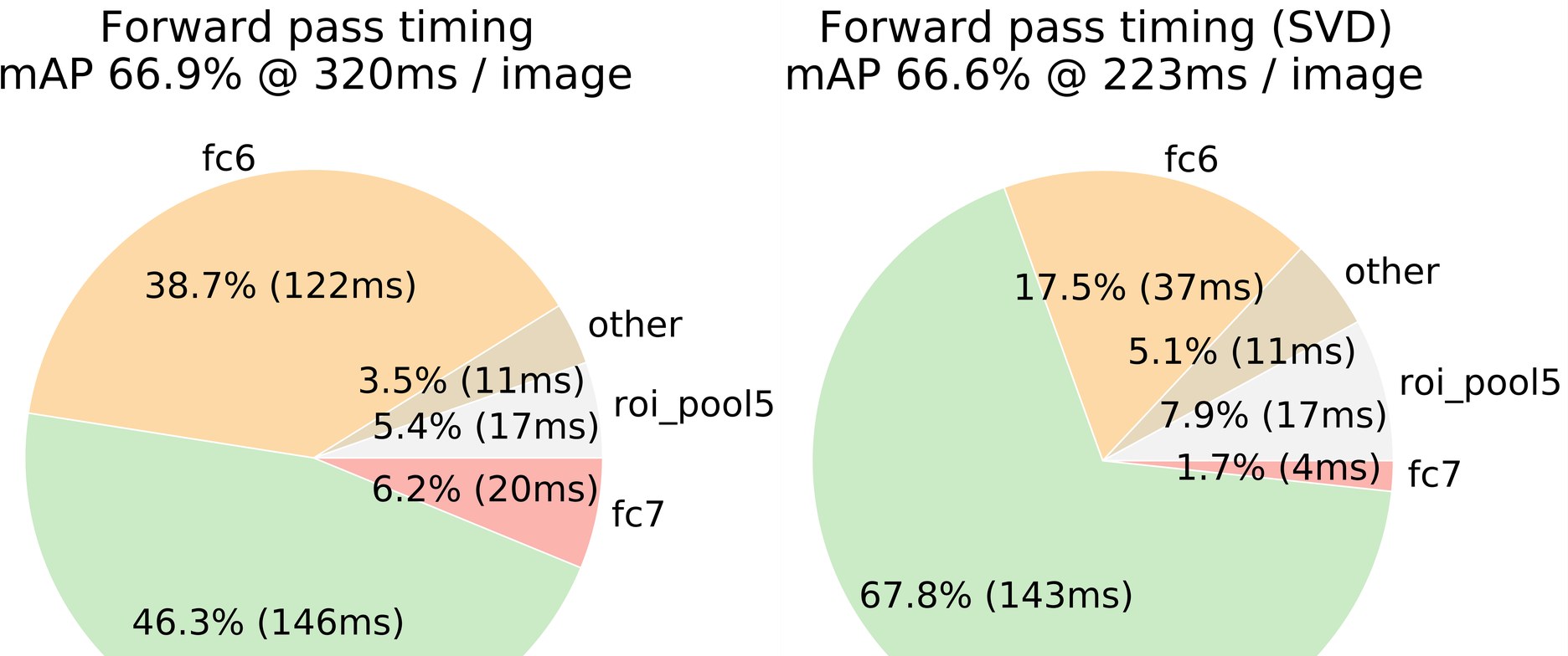
Figure 2: Timing for VGG16 before and after truncated SVD. Before SVD, fully connected layers fc6 and fc7 take 45% of the time.
图 2:截断 SVD 前后 VGG16 的耗时。做 SVD 之前,全连接层 fc6 和 fc7 占总时间的 45%。
4.5 Which layers to fine-tune?
4.5 应该微调哪些层?
For the less deep networks considered in the SPPnet paper [11], fine-tuning only the fully connected layers appeared to be sufficient for good accuracy. We hypothesized that this result would not hold for very deep networks. To validate that fine-tuning the conv layers is important for VGG16, we use Fast R-CNN to fine-tune, but freeze the thirteen conv layers so that only the fully connected layers learn. This ablation emulates single-scale SPPnet training and decreases mAP from 66.9% to 61.4% (Table 5). This experiment verifies our hypothesis: training through the RoI pooling layer is important for very deep nets.
对 SPPnet 论文 [11] 中那些不那么深的网络,只微调全连接层似乎就足以得到好精度。我们猜想,这个结论对很深的网络并不成立。为了验证微调卷积层对 VGG16 很重要,我们仍用 Fast R-CNN 做微调,但冻结十三层卷积,只让全连接层学习。这一消融相当于单尺度的 SPPnet 训练,并把 mAP 从 66.9% 降到 61.4%(表 5)。实验证实了我们的猜想:对很深的网络,把训练做到穿过 RoI 池化层是重要的。
| layers that are fine-tuned in model L | SPPnet L | |||
|---|---|---|---|---|
| fc6 | conv3_1 | conv2_1 | fc6 | |
| VOC07 mAP | 61.4 | 66.9 | 67.2 | 63.1 |
| test rate (s/im) | 0.32 | 0.32 | 0.32 | 2.3 |
Table 5: Effect of restricting which layers are fine-tuned for VGG16. Fine-tuning fc6 emulates the SPPnet training algorithm [11], but using a single scale. SPPnet L results were obtained using five scales, at a significant (7) speed cost.
| 模型 L 中被微调的层 | SPPnet L | |||
|---|---|---|---|---|
| fc6 | conv3_1 | conv2_1 | fc6 | |
| VOC07 mAP | 61.4 | 66.9 | 67.2 | 63.1 |
| 测试速率(秒/图) | 0.32 | 0.32 | 0.32 | 2.3 |
表 5:限制 VGG16 中哪些层被微调的影响。微调 fc6 相当于 [11] 中的 SPPnet 训练算法,但使用单尺度。SPPnet L 的结果是在五个尺度上得到的,速度上要付出显著代价(慢 7 倍)。
Does this mean that all conv layers should be fine-tuned? In short, no. In the smaller networks (S and M) we find that conv1 is generic and task independent (a well-known fact [14]). Allowing conv1 to learn, or not, has no meaningful effect on mAP. For VGG16, we found it only necessary to update layers from conv3_1 and up (9 of the 13 conv layers). This observation is pragmatic: (1) updating from conv2_1 slows training by 1.3 (12.5 vs. 9.5 hours) compared to learning from conv3_1; and (2) updating from conv1_1 over-runs GPU memory. The difference in mAP when learning from conv2_1 up was only points (Table 5, last column). All Fast R-CNN results in this paper using VGG16 fine-tune layers conv3_1 and up; all experiments with models S and M fine-tune layers conv2 and up.
这是否意味着所有卷积层都应该微调?简短的答案是不必。在较小的网络(S 和 M)上,我们发现 conv1 是通用的、与任务无关的(这是一个广为人知的事实 [14])。让 conv1 学习与否,对 mAP 没有实质影响。对 VGG16,我们发现只需更新从 conv3_1 往上的层(13 层卷积中的 9 层)。这一观察有实际意义:(1)从 conv2_1 开始更新,训练会比从 conv3_1 开始慢 1.3 倍(12.5 小时对 9.5 小时);(2)从 conv1_1 开始更新会超出 GPU 显存。从 conv2_1 往上学习时,mAP 只高 0.3 个点(表 5 最后一列)。本文所有使用 VGG16 的 Fast R-CNN 结果都微调 conv3_1 及以上的层;所有模型 S 和 M 的实验都微调 conv2 及以上的层。
| S | M | L | ||||||||||
|---|---|---|---|---|---|---|---|---|---|---|---|---|
| multi-task training? | ✓ | ✓ | ✓ | ✓ | ✓ | ✓ | ||||||
| stage-wise training? | ✓ | ✓ | ✓ | |||||||||
| test-time bbox reg? | ✓ | ✓ | ✓ | ✓ | ✓ | ✓ | ||||||
| VOC07 mAP | 52.2 | 53.3 | 54.6 | 57.1 | 54.7 | 55.5 | 56.6 | 59.2 | 62.6 | 63.4 | 64.0 | 66.9 |
Table 6: Multi-task training (forth column per group) improves mAP over piecewise training (third column per group).
| S | M | L | ||||||||||
|---|---|---|---|---|---|---|---|---|---|---|---|---|
| 是否多任务训练? | √ | √ | √ | √ | √ | √ | ||||||
| 是否分阶段训练? | √ | √ | √ | |||||||||
| 测试时是否做边界框回归? | √ | √ | √ | √ | √ | √ | ||||||
| VOC07 mAP | 52.2 | 53.3 | 54.6 | 57.1 | 54.7 | 55.5 | 56.6 | 59.2 | 62.6 | 63.4 | 64.0 | 66.9 |
表 6:多任务训练(每组第四列)相对分段训练(每组第三列)提高了 mAP。
5 Design evaluation
5 设计评估
We conducted experiments to understand how Fast R-CNN compares to R-CNN and SPPnet, as well as to evaluate design decisions. Following best practices, we performed these experiments on the PASCAL VOC07 dataset.
我们做了一组实验,既要弄清 Fast R-CNN 与 R-CNN、SPPnet 相比如何,也要评估各项设计选择。按照常见做法,这些实验都在 PASCAL VOC07 数据集上进行。
5.1 Does multi-task training help?
5.1 多任务训练有没有帮助?
Multi-task training is convenient because it avoids managing a pipeline of sequentially-trained tasks. But it also has the potential to improve results because the tasks influence each other through a shared representation (the ConvNet) [2]. Does multi-task training improve object detection accuracy in Fast R-CNN?
多任务训练很方便,因为它避免管理一条按顺序训练的任务流水线。它也有可能提高结果,因为各个任务会通过共享表示(卷积网络)相互影响 [2]。多任务训练能否提高 Fast R-CNN 的目标检测精度?
To test this question, we train baseline networks that use only the classification loss, , in Eq. 1 (i.e., setting ). These baselines are printed for models S, M, and L in the first column of each group in Table 6. Note that these models do not have bounding-box regressors. Next (second column per group), we take networks that were trained with the multi-task loss (Eq. 1, ), but we disable bounding-box regression at test time. This isolates the networks’ classification accuracy and allows an apples-to-apples comparison with the baseline networks.
为了检验这个问题,我们训练只使用式 1 中分类损失 的基线网络(也就是令 )。这些基线对应于表 6 中模型 S、M 和 L 每组的第一列。注意,这些模型没有边界框回归器。接下来(每组第二列),我们取用多任务损失(式 1,)训练好的网络,但在测试时关掉边界框回归。这样就单独衡量网络的分类精度,可以与基线网络做对等比较。
Across all three networks we observe that multi-task training improves pure classification accuracy relative to training for classification alone. The improvement ranges from to mAP points, showing a consistent positive effect from multi-task learning.
在全部三个网络上,我们都观察到:相对只训练分类,多任务训练提高了纯粹的分类精度。提升幅度在 到 个 mAP 点之间,说明多任务学习有稳定的正向作用。
Finally, we take the baseline models (trained with only the classification loss), tack on the bounding-box regression layer, and train them with while keeping all other network parameters frozen. The third column in each group shows the results of this stage-wise training scheme: mAP improves over column one, but stage-wise training underperforms multi-task training (forth column per group).
最后,我们取只按分类损失训练的基线模型,接上边界框回归层,在冻结其余网络参数的情况下用 训练它们。每组第三列给出这种分阶段训练方案的结果:mAP 比第一列有提高,但分阶段训练仍不如多任务训练(每组第四列)。
5.2 Scale invariance: to brute force or finesse?
5.2 尺度不变性:靠蛮力还是靠技巧?
We compare two strategies for achieving scale-invariant object detection: brute-force learning (single scale) and image pyramids (multi-scale). In either case, we define the scale of an image to be the length of its shortest side.
我们比较了两种实现尺度不变目标检测的策略:蛮力学习(单尺度)和图像金字塔(多尺度)。无论哪种情形,我们都把一幅图像的尺度 定义为其短边的长度。
All single-scale experiments use pixels; may be less than for some images as we cap the longest image side at pixels and maintain the image’s aspect ratio. These values were selected so that VGG16 fits in GPU memory during fine-tuning. The smaller models are not memory bound and can benefit from larger values of ; however, optimizing for each model is not our main concern. We note that PASCAL images are pixels on average and thus the single-scale setting typically upsamples images by a factor of 1.6. The average effective stride at the RoI pooling layer is thus pixels.
全部单尺度实验使用 像素;对某些图像, 可能小于 ,因为我们把最长边限制在 像素,并保持宽高比。这样取值是为了让 VGG16 在微调时放得进 GPU 显存。较小的模型不受显存限制,本可以从更大的 中受益;不过,为每个模型单独优化 并不是我们的主要关心。需要说明的是,PASCAL 图像的平均尺寸约为 像素,因此单尺度设定通常会把图像上采样约 1.6 倍。于是 RoI 池化层上的平均有效步幅约为 10 像素。
In the multi-scale setting, we use the same five scales specified in [11] () to facilitate comparison with SPPnet. However, we cap the longest side at pixels to avoid exceeding GPU memory.
在多尺度设定中,为了便于与 SPPnet 比较,我们使用 [11] 中指定的同样五个尺度()。不过,为了不超出 GPU 显存,我们把最长边限制在 像素。
| SPPnet ZF | S | M | L | ||||
|---|---|---|---|---|---|---|---|
| scales | 1 | 5 | 1 | 5 | 1 | 5 | 1 |
| test rate (s/im) | 0.14 | 0.38 | 0.10 | 0.39 | 0.15 | 0.64 | 0.32 |
| VOC07 mAP | 58.0 | 59.2 | 57.1 | 58.4 | 59.2 | 60.7 | 66.9 |
Table 7: Multi-scale vs. single scale. SPPnet ZF (similar to model S) results are from [11]. Larger networks with a single-scale offer the best speed / accuracy tradeoff. (L cannot use multi-scale in our implementation due to GPU memory constraints.)
| SPPnet ZF | S | M | L | ||||
|---|---|---|---|---|---|---|---|
| 尺度数 | 1 | 5 | 1 | 5 | 1 | 5 | 1 |
| 测试速率(秒/图) | 0.14 | 0.38 | 0.10 | 0.39 | 0.15 | 0.64 | 0.32 |
| VOC07 mAP | 58.0 | 59.2 | 57.1 | 58.4 | 59.2 | 60.7 | 66.9 |
表 7:多尺度与单尺度的比较。SPPnet ZF(与模型 S 类似)的结果来自 [11]。较大网络配单尺度,给出了最好的速度/精度权衡。(在我们的实现中,L 受 GPU 显存限制,不能使用多尺度。)
Table 7 shows models S and M when trained and tested with either one or five scales. Perhaps the most surprising result in [11] was that single-scale detection performs almost as well as multi-scale detection. Our findings confirm their result: deep ConvNets are adept at directly learning scale invariance. The multi-scale approach offers only a small increase in mAP at a large cost in compute time (Table 7). In the case of VGG16 (model L), we are limited to using a single scale by implementation details. Yet it achieves a mAP of 66.9%, which is slightly higher than the 66.0% reported for R-CNN [10], even though R-CNN uses “infinite” scales in the sense that each proposal is warped to a canonical size.
表 7 给出了模型 S 和 M 在一个或五个尺度上训练和测试的结果。[11] 中或许最令人意外的结果是:单尺度检测几乎和多尺度检测一样好。我们的发现证实了这一点:深层卷积网络很善于直接学习尺度不变性。多尺度方法只带来很小的 mAP 提升,却要付出很大的计算代价(表 7)。对 VGG16(模型 L),受实现细节限制,我们只能使用单尺度。即便如此,它仍达到 66.9% 的 mAP,略高于 R-CNN [10] 所报告的 66.0%,尽管 R-CNN 在某种意义上使用了“无穷多”尺度——每个提议都会被扭曲到一个标准尺寸。
Since single-scale processing offers the best tradeoff between speed and accuracy, especially for very deep models, all experiments outside of this sub-section use single-scale training and testing with pixels.
由于单尺度处理在速度和精度之间给出了最好的权衡,对很深的模型尤其如此,本小节以外的全部实验都使用 像素的单尺度训练和测试。
5.3 Do we need more training data?
5.3 我们需要更多训练数据吗?
A good object detector should improve when supplied with more training data. Zhu et al. [24] found that DPM [8] mAP saturates after only a few hundred to thousand training examples. Here we augment the VOC07 trainval set with the VOC12 trainval set, roughly tripling the number of images to 16.5k, to evaluate Fast R-CNN. Enlarging the training set improves mAP on VOC07 test from 66.9% to 70.0% (Table 1). When training on this dataset we use 60k mini-batch iterations instead of 40k.
一个好的目标检测器,在得到更多训练数据时应当还能提高。Zhu 等人 [24] 发现,DPM [8] 的 mAP 在几百到一千个训练样本之后就会饱和。这里我们把 VOC12 trainval 加进 VOC07 trainval,把图像数大约扩大到三倍,达到 1.65 万,以评估 Fast R-CNN。扩大训练集后,VOC07 测试集上的 mAP 从 66.9% 提高到 70.0%(表 1)。在这套数据上训练时,我们使用 6 万次小批量迭代,而不是 4 万次。
We perform similar experiments for VOC10 and 2012, for which we construct a dataset of 21.5k images from the union of VOC07 trainval, test, and VOC12 trainval. When training on this dataset, we use 100k SGD iterations and lower the learning rate by each 40k iterations (instead of each 30k). For VOC10 and 2012, mAP improves from 66.1% to 68.8% and from 65.7% to 68.4%, respectively.
我们对 VOC10 和 2012 做了类似实验,把 VOC07 的 trainval、test 与 VOC12 trainval 合并,构成 2.15 万张图的数据集。在这套数据上训练时,我们使用 10 万次 SGD 迭代,并且每隔 4 万次(而不是每隔 3 万次)把学习率乘以 。对 VOC10 和 2012,mAP 分别从 66.1% 提高到 68.8%,从 65.7% 提高到 68.4%。
5.4 Do SVMs outperform softmax?
5.4 SVM 是否优于 softmax?
Fast R-CNN uses the softmax classifier learnt during fine-tuning instead of training one-vs-rest linear SVMs post-hoc, as was done in R-CNN and SPPnet. To understand the impact of this choice, we implemented post-hoc SVM training with hard negative mining in Fast R-CNN. We use the same training algorithm and hyper-parameters as in R-CNN.
Fast R-CNN 使用微调过程中学到的 softmax 分类器,而不再像 R-CNN 和 SPPnet 那样事后训练一对多的线性 SVM。为了理解这一选择的影响,我们在 Fast R-CNN 中实现了带难负例挖掘的事后 SVM 训练。训练算法和超参数与 R-CNN 相同。
| method | classifier | S | M | L |
|---|---|---|---|---|
| R-CNN [9, 10] | SVM | 58.5 | 60.2 | 66.0 |
| FRCN [ours] | SVM | 56.3 | 58.7 | 66.8 |
| FRCN [ours] | softmax | 57.1 | 59.2 | 66.9 |
Table 8: Fast R-CNN with softmax vs. SVM (VOC07 mAP).
| 方法 | 分类器 | S | M | L |
|---|---|---|---|---|
| R-CNN [9, 10] | SVM | 58.5 | 60.2 | 66.0 |
| FRCN [本文] | SVM | 56.3 | 58.7 | 66.8 |
| FRCN [本文] | softmax | 57.1 | 59.2 | 66.9 |
表 8:Fast R-CNN 使用 softmax 与使用 SVM 的比较(VOC07 mAP)。
Table 8 shows softmax slightly outperforming SVM for all three networks, by to mAP points. This effect is small, but it demonstrates that “one-shot” fine-tuning is sufficient compared to previous multi-stage training approaches. We note that softmax, unlike one-vs-rest SVMs, introduces competition between classes when scoring a RoI.
表 8 显示,对全部三个网络,softmax 都略优于 SVM,幅度为 到 个 mAP 点。这一效应不大,但说明与此前的多阶段训练相比,“一次完成”的微调已经足够。还需要指出,与一对多 SVM 不同,softmax 在给一个 RoI 打分时会引入类别之间的竞争。
5.5 Are more proposals always better?
5.5 提议越多越好吗?
There are (broadly) two types of object detectors: those that use a sparse set of object proposals (e.g., selective search [21]) and those that use a dense set (e.g., DPM [8]). Classifying sparse proposals is a type of cascade [22] in which the proposal mechanism first rejects a vast number of candidates leaving the classifier with a small set to evaluate. This cascade improves detection accuracy when applied to DPM detections [21]. We find evidence that the proposal-classifier cascade also improves Fast R-CNN accuracy.
目标检测器大体上有两类:一类使用稀疏的物体提议(例如选择性搜索 [21]),一类使用稠密集合(例如 DPM [8])。给稀疏提议分类是一种级联 [22]:提议机制先拒绝掉海量候选,只给分类器留下一小批去评估。这种级联用在 DPM 检测上时能提高精度 [21]。我们找到的证据表明,提议–分类器级联也能提高 Fast R-CNN 的精度。
Using selective search’s quality mode, we sweep from 1k to 10k proposals per image, each time re-training and re-testing model M. If proposals serve a purely computational role, increasing the number of proposals per image should not harm mAP.
使用选择性搜索的质量模式,我们把每张图的提议数从 1 千扫到 1 万,每次都重新训练并测试模型 M。如果提议只起纯粹的计算作用,增加每张图的提议数就不应当损害 mAP。
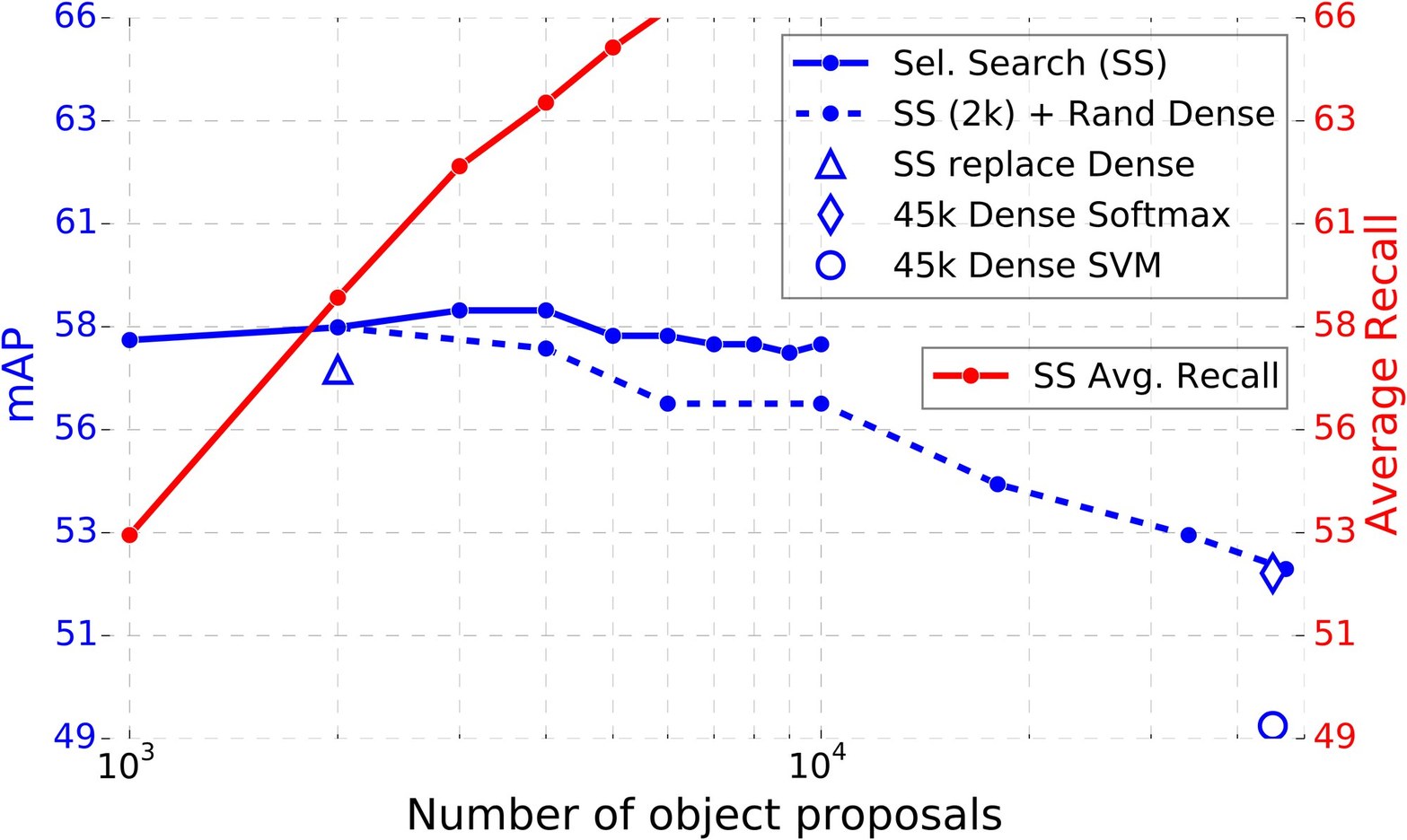
Figure 3: VOC07 test mAP and AR for various proposal schemes.
图 3:不同提议方案下 VOC07 测试集的 mAP 与平均召回率(AR)。
We find that mAP rises and then falls slightly as the proposal count increases (Fig. 3, solid blue line). This experiment shows that swamping the deep classifier with more proposals does not help, and even slightly hurts, accuracy.
我们发现,随着提议数增加,mAP 先升后略降(图 3,实心蓝线)。这一实验表明,用更多提议去淹没深层分类器并无帮助,甚至还会轻微损害精度。
This result is difficult to predict without actually running the experiment. The state-of-the-art for measuring object proposal quality is Average Recall (AR) [12]. AR correlates well with mAP for several proposal methods using R-CNN, when using a fixed number of proposals per image. Fig. 3 shows that AR (solid red line) does not correlate well with mAP as the number of proposals per image is varied. AR must be used with care; higher AR due to more proposals does not imply that mAP will increase. Fortunately, training and testing with model M takes less than 2.5 hours. Fast R-CNN thus enables efficient, direct evaluation of object proposal mAP, which is preferable to proxy metrics.
若不真正做实验,这一结果很难预见到。衡量物体提议质量的当时最优指标是平均召回率(AR)[12]。在每张图使用固定数量提议时,对若干与 R-CNN 搭配的提议方法,AR 与 mAP 相关性很好。图 3 显示,当每张图的提议数变化时,AR(实心红线)与 mAP 的相关性并不好。使用 AR 时必须小心:因提议变多而升高的 AR,并不意味着 mAP 也会升高。好在用模型 M 训练和测试只需不到 2.5 小时。因此 Fast R-CNN 使直接、高效地评估物体提议的 mAP 成为可能,这比使用替代指标更可取。
We also investigate Fast R-CNN when using densely generated boxes (over scale, position, and aspect ratio), at a rate of about 45k boxes / image. This dense set is rich enough that when each selective search box is replaced by its closest (in IoU) dense box, mAP drops only 1 point (to 57.7%, Fig. 3, blue triangle).
我们还考察了 Fast R-CNN 在使用稠密生成框(覆盖尺度、位置和宽高比)时的表现,大约每张图 4.5 万个框。这组稠密框足够丰富:若把每个选择性搜索框替换成与它交并比最接近的稠密框,mAP 只下降 1 个点(到 57.7%,图 3,蓝色三角)。
The statistics of the dense boxes differ from those of selective search boxes. Starting with 2k selective search boxes, we test mAP when adding a random sample of dense boxes. For each experiment we re-train and re-test model M. When these dense boxes are added, mAP falls more strongly than when adding more selective search boxes, eventually reaching 53.0%.
稠密框的统计性质与选择性搜索框不同。我们从 2 千个选择性搜索框出发,再加入随机采样的 个稠密框,测试此时的 mAP。每个实验都重新训练并测试模型 M。加入这些稠密框后,mAP 的下降比继续加入更多选择性搜索框更明显,最终降到 53.0%。
We also train and test Fast R-CNN using only dense boxes (45k / image). This setting yields a mAP of 52.9% (blue diamond). Finally, we check if SVMs with hard negative mining are needed to cope with the dense box distribution. SVMs do even worse: 49.3% (blue circle).
我们还只用稠密框(每张图 4.5 万个)训练和测试 Fast R-CNN。这一设定得到的 mAP 为 52.9%(蓝色菱形)。最后,我们检查是否需要带难负例挖掘的 SVM 来应对稠密框的分布。SVM 的结果更差:49.3%(蓝色圆点)。
5.6 Preliminary MS COCO results
5.6 MS COCO 上的初步结果
We applied Fast R-CNN (with VGG16) to the MS COCO dataset [18] to establish a preliminary baseline. We trained on the 80k image training set for 240k iterations and evaluated on the “test-dev” set using the evaluation server. The PASCAL-style mAP is 35.9%; the new COCO-style AP, which also averages over IoU thresholds, is 19.7%.
我们把 Fast R-CNN(使用 VGG16)用到 MS COCO 数据集 [18] 上,给出一个初步基线。我们在 8 万张训练图上训练 24 万次迭代,并用评测服务器在 “test-dev” 集上评估。PASCAL 风格的 mAP 为 35.9%;同时对交并比阈值再取平均的新 COCO 风格 AP 为 19.7%。
6 Conclusion
6 结论
This paper proposes Fast R-CNN, a clean and fast update to R-CNN and SPPnet. In addition to reporting state-of-the-art detection results, we present detailed experiments that we hope provide new insights. Of particular note, sparse object proposals appear to improve detector quality. This issue was too costly (in time) to probe in the past, but becomes practical with Fast R-CNN. Of course, there may exist yet undiscovered techniques that allow dense boxes to perform as well as sparse proposals. Such methods, if developed, may help further accelerate object detection.
本文提出 Fast R-CNN,它是对 R-CNN 和 SPPnet 的一次干净而快速的更新。除了报告当时最好的检测结果,我们还给出了希望能带来新认识的详细实验。特别值得注意的是,稀疏的物体提议似乎能提高检测器质量。这件事过去因耗时太多而难以细究,但有了 Fast R-CNN 就变得可行。当然,也许还存在尚未发现的技术,能让稠密框达到与稀疏提议相当的表现。若这类方法被发展出来,或许会进一步加快目标检测。
Acknowledgements.
I thank Kaiming He, Larry Zitnick, and Piotr Dollár for helpful discussions and encouragement.
致谢。
我感谢 Kaiming He、Larry Zitnick 和 Piotr Dollár 的讨论与鼓励。
Footnotes
脚注
- All timings use one Nvidia K40 GPU overclocked to 875 MHz.
- 所有计时均在一块超频至 875 MHz 的 Nvidia K40 GPU 上测得。
- http://host.robots.ox.ac.uk:8080/leaderboard (accessed April 18, 2015)
- http://host.robots.ox.ac.uk:8080/leaderboard(查阅于 2015 年 4 月 18 日)
References
参考文献
[1] J. Carreira, R. Caseiro, J. Batista, and C. Sminchisescu. Semantic segmentation with second-order pooling. In ECCV , 2012.
[2] R. Caruana. Multitask learning. Machine learning , 28(1), 1997.
[3] K. Chatfield, K. Simonyan, A. Vedaldi, and A. Zisserman. Return of the devil in the details: Delving deep into convolutional nets. In BMVC , 2014.
[4] J. Deng, W. Dong, R. Socher, L.-J. Li, K. Li, and L. Fei-Fei. ImageNet: A large-scale hierarchical image database. In CVPR , 2009.
[5] E. Denton, W. Zaremba, J. Bruna, Y. LeCun, and R. Fergus. Exploiting linear structure within convolutional networks for efficient evaluation. In NIPS , 2014.
[6] D. Erhan, C. Szegedy, A. Toshev, and D. Anguelov. Scalable object detection using deep neural networks. In CVPR , 2014.
[7] M. Everingham, L. Van Gool, C. K. I. Williams, J. Winn, and A. Zisserman. The PASCAL Visual Object Classes (VOC) Challenge. IJCV , 2010.
[8] P. Felzenszwalb, R. Girshick, D. McAllester, and D. Ramanan. Object detection with discriminatively trained part based models. TPAMI , 2010.
[9] R. Girshick, J. Donahue, T. Darrell, and J. Malik. Rich feature hierarchies for accurate object detection and semantic segmentation. In CVPR , 2014.
[10] R. Girshick, J. Donahue, T. Darrell, and J. Malik. Region-based convolutional networks for accurate object detection and segmentation. TPAMI , 2015.
[11] K. He, X. Zhang, S. Ren, and J. Sun. Spatial pyramid pooling in deep convolutional networks for visual recognition. In ECCV , 2014.
[12] J. H. Hosang, R. Benenson, P. Dollár, and B. Schiele. What makes for effective detection proposals? arXiv preprint arXiv:1502.05082 , 2015.
[13] Y. Jia, E. Shelhamer, J. Donahue, S. Karayev, J. Long, R. Girshick, S. Guadarrama, and T. Darrell. Caffe: Convolutional architecture for fast feature embedding. In Proc. of the ACM International Conf. on Multimedia , 2014.
[14] A. Krizhevsky, I. Sutskever, and G. Hinton. ImageNet classification with deep convolutional neural networks. In NIPS , 2012.
[15] S. Lazebnik, C. Schmid, and J. Ponce. Beyond bags of features: Spatial pyramid matching for recognizing natural scene categories. In CVPR , 2006.
[16] Y. LeCun, B. Boser, J. Denker, D. Henderson, R. Howard, W. Hubbard, and L. Jackel. Backpropagation applied to handwritten zip code recognition. Neural Comp. , 1989.
[17] M. Lin, Q. Chen, and S. Yan. Network in network. In ICLR , 2014.
[18] T. Lin, M. Maire, S. Belongie, L. Bourdev, R. Girshick, J. Hays, P. Perona, D. Ramanan, P. Dollár, and C. L. Zitnick. Microsoft COCO: common objects in context. arXiv e-prints , arXiv:1405.0312 [cs.CV], 2014.
[19] P. Sermanet, D. Eigen, X. Zhang, M. Mathieu, R. Fergus, and Y. LeCun. OverFeat: Integrated Recognition, Localization and Detection using Convolutional Networks. In ICLR , 2014.
[20] K. Simonyan and A. Zisserman. Very deep convolutional networks for large-scale image recognition. In ICLR , 2015.
[21] J. Uijlings, K. van de Sande, T. Gevers, and A. Smeulders. Selective search for object recognition. IJCV , 2013.
[22] P. Viola and M. Jones. Rapid object detection using a boosted cascade of simple features. In CVPR , 2001.
[23] J. Xue, J. Li, and Y. Gong. Restructuring of deep neural network acoustic models with singular value decomposition. In Interspeech , 2013.
[24] X. Zhu, C. Vondrick, D. Ramanan, and C. Fowlkes. Do we need more training data or better models for object detection? In BMVC , 2012.
[25] Y. Zhu, R. Urtasun, R. Salakhutdinov, and S. Fidler. segDeepM: Exploiting segmentation and context in deep neural networks for object detection. In CVPR , 2015.