Explaining and Harnessing Adversarial Examples

解释并利用对抗样本

Ian J. Goodfellow    Jonathon Shlens & Christian Szegedy Affiliation:  Google Inc., Mountain View, CA Email:  {goodfellow,shlens,szegedy}@google.com

Abstract

摘要

Several machine learning models, including neural networks, consistently misclassify adversarial examples—inputs formed by applying small but intentionally worst-case perturbations to examples from the dataset, such that the perturbed input results in the model outputting an incorrect answer with high confidence. Early attempts at explaining this phenomenon focused on nonlinearity and overfitting. We argue instead that the primary cause of neural networks’ vulnerability to adversarial perturbation is their linear nature. This explanation is supported by new quantitative results while giving the first explanation of the most intriguing fact about them: their generalization across architectures and training sets. Moreover, this view yields a simple and fast method of generating adversarial examples. Using this approach to provide examples for adversarial training, we reduce the test set error of a maxout network on the MNIST dataset.

包括神经网络在内的若干机器学习模型，会一贯地误分类 对抗样本：这类输入是在数据集中的样本上施加虽小、却故意按最坏情况选择的扰动后得到的，扰动后的输入会让模型以很高的把握给出错误答案。早期解释这一现象的尝试，多把原因放在非线性和过拟合上。我们则认为，神经网络容易被对抗扰动击中，首要原因是它们的线性本质。这一解释既有新的定量结果作为支持，也第一次说明了它们最令人费解的一点：对抗样本可以在不同结构和不同训练集之间泛化。不仅如此，这一看法还给出一种简单、快速的对抗样本生成方法。我们用这种方法为对抗训练提供样本，降低了 maxout 网络在 MNIST 数据集上的测试误差。

1 Introduction

1 引言

Szegedy et al. (2014b) made an intriguing discovery: several machine learning models, including state-of-the-art neural networks, are vulnerable to adversarial examples. That is, these machine learning models misclassify examples that are only slightly different from correctly classified examples drawn from the data distribution. In many cases, a wide variety of models with different architectures trained on different subsets of the training data misclassify the same adversarial example. This suggests that adversarial examples expose fundamental blind spots in our training algorithms.

Szegedy 等人 (2014b) 有一项引人注目的发现：包括当时最好的神经网络在内，若干机器学习模型都容易受到 对抗样本 的攻击。也就是说，这些模型会把一些例子分错，而这些例子与从数据分布中抽出、本来分对的例子只差很小一点。在许多情形下，结构不同、又在训练集的不同子集上训练的各种各样模型，会把同一个对抗样本分错。这说明，对抗样本暴露的是我们训练算法中根本性的盲区。

The cause of these adversarial examples was a mystery, and speculative explanations have suggested it is due to extreme nonlinearity of deep neural networks, perhaps combined with insufficient model averaging and insufficient regularization of the purely supervised learning problem. We show that these speculative hypotheses are unnecessary. Linear behavior in high-dimensional spaces is sufficient to cause adversarial examples. This view enables us to design a fast method of generating adversarial examples that makes adversarial training practical. We show that adversarial training can provide an additional regularization benefit beyond that provided by using dropout (Srivastava et al., 2014) alone. Generic regularization strategies such as dropout, pretraining, and model averaging do not confer a significant reduction in a model’s vulnerability to adversarial examples, but changing to nonlinear model families such as RBF networks can do so.

这些对抗样本的成因一度是个谜。带推测的解释认为，原因是深度神经网络极端的非线性，或许再叠加上模型平均不够、以及纯监督学习问题的正则不够。我们表明，这些推测性的假说并不是必要的。高维空间中的线性行为，就足以产生对抗样本。这一看法让我们能够设计出一种快速生成对抗样本的方法，从而使对抗训练变得可行。我们表明，对抗训练能在 dropout (Srivastava 等人, 2014) 之外再提供一份正则收益。dropout、预训练和模型平均这类通用正则策略，并不能显著降低模型对对抗样本的脆弱性；改用 RBF 网络这类非线性模型家族，则可以做到这一点。

Our explanation suggests a fundamental tension between designing models that are easy to train due to their linearity and designing models that use nonlinear effects to resist adversarial perturbation. In the long run, it may be possible to escape this tradeoff by designing more powerful optimization methods that can succesfully train more nonlinear models.

我们的解释提示了一种根本性的张力：一边是把模型设计得足够线性、从而容易训练，另一边是利用非线性效应来抵抗对抗扰动。从长远看，或许可以通过设计更有力的优化方法、成功训练非线性更强的模型，来摆脱这一权衡。

2 Related work

2 相关工作

Szegedy et al. (2014b) demonstrated a variety of intriguing properties of neural networks and related models. Those most relevant to this paper include:

Szegedy 等人 (2014b) 展示了神经网络及相关模型的许多有趣性质。与本文最相关的包括：

• • Box-constrained L-BFGS can reliably find adversarial examples.

• 带盒约束的 L-BFGS 可以可靠地找到对抗样本。

• • On some datasets, such as ImageNet (Deng et al., 2009), the adversarial examples were so close to the original examples that the differences were indistinguishable to the human eye.

• 在某些数据集上，例如 ImageNet (Deng 等人, 2009)，对抗样本与原例靠得非常近，差异用人眼无法分辨。

• • The same adversarial example is often misclassified by a variety of classifiers with different architectures or trained on different subsets of the training data.

• 同一个对抗样本，常常会被结构不同、或在训练集不同子集上训练的多种分类器一齐分错。

• • Shallow softmax regression models are also vulnerable to adversarial examples.

• 浅层 softmax 回归模型同样容易受到对抗样本的攻击。

• • Training on adversarial examples can regularize the model—however, this was not practical at the time due to the need for expensive constrained optimization in the inner loop.

• 在对抗样本上训练可以对模型起正则作用——不过在当时这并不实用，因为内层循环需要昂贵的约束优化。

These results suggest that classifiers based on modern machine learning techniques, even those that obtain excellent performance on the test set, are not learning the true underlying concepts that determine the correct output label. Instead, these algorithms have built a Potemkin village that works well on naturally occuring data, but is exposed as a fake when one visits points in space that do not have high probability in the data distribution. This is particularly disappointing because a popular approach in computer vision is to use convolutional network features as a space where Euclidean distance approximates perceptual distance. This resemblance is clearly flawed if images that have an immeasurably small perceptual distance correspond to completely different classes in the network’s representation.

这些结果说明，基于现代机器学习技术的分类器，即便在测试集上表现极好，也并没有学到决定正确输出标签的那些真正底层概念。相反，这些算法搭起的是一座波将金村庄：在自然出现的数据上运转良好，可一旦走到数据分布里概率不高的位置，假象就会被揭穿。这尤其令人失望，因为计算机视觉里一种流行做法，是把卷积网络特征当作欧氏距离近似感知距离的空间。如果两张在感知距离上小到几乎无法测量的图像，在网络表征里却对应完全不同的类别，这种相似性显然是靠不住的。

These results have often been interpreted as being a flaw in deep networks in particular, even though linear classifiers have the same problem. We regard the knowledge of this flaw as an opportunity to fix it. Indeed,  Gu & Rigazio (2014) and  Chalupka et al. (2014) have already begun the first steps toward designing models that resist adversarial perturbation, though no model has yet succesfully done so while maintaining state of the art accuracy on clean inputs.

这些结果常常被理解成深度网络特有的缺陷，尽管线性分类器也有同样的问题。我们把知道这一缺陷看成一次修好它的机会。事实上，Gu 与 Rigazio (2014) 以及 Chalupka 等人 (2014) 已经迈出了设计能够抵抗对抗扰动的模型的第一步，不过还没有哪个模型在保持干净输入上的前沿精度的同时，真正做到了这一点。

3 The linear explanation of adversarial examples

3 对抗样本的线性解释

We start with explaining the existence of adversarial examples for linear models.

我们先从解释线性模型为何会存在对抗样本开始。

In many problems, the precision of an individual input feature is limited. For example, digital images often use only 8 bits per pixel so they discard all information below $1/255$ of the dynamic range. Because the precision of the features is limited, it is not rational for the classifier to respond differently to an input ${\bm{x}}$ than to an adversarial input $\tilde{{\bm{x}}}={\bm{x}}+{\bm{\eta}}$ if every element of the perturbation ${\bm{\eta}}$ is smaller than the precision of the features. Formally, for problems with well-separated classes, we expect the classifier to assign the same class to ${\bm{x}}$ and $\tilde{{\bm{x}}}$ so long as $||{\bm{\eta}}||_{\infty}<{\epsilon}$, where ${\epsilon}$ is small enough to be discarded by the sensor or data storage apparatus associated with our problem.

在许多问题里，单个输入特征的精度是有限的。例如，数字图像常常每个像素只用 8 比特，因此会丢弃动态范围中低于 $1/255$ 的全部信息。由于特征精度有限，如果扰动 ${\bm{\eta}}$ 的每个元素都小于特征精度，分类器对输入 ${\bm{x}}$ 和对对抗输入 $\tilde{{\bm{x}}}={\bm{x}}+{\bm{\eta}}$ 做出不同反应，就是不合理的。形式化地说，对于类别分得比较开的问题，只要 $||{\bm{\eta}}||_{\infty}<{\epsilon}$，我们就期望分类器给 ${\bm{x}}$ 和 $\tilde{{\bm{x}}}$ 分到同一类，其中 ${\epsilon}$ 要小到能被与该问题相关的传感器或数据存储装置丢掉。

Consider the dot product between a weight vector ${\bm{w}}$ and an adversarial example $\tilde{{\bm{x}}}$:

考虑权重向量 ${\bm{w}}$ 与对抗样本 $\tilde{{\bm{x}}}$ 的点积：

$${\bm{w}}^{\top}\tilde{{\bm{x}}}={\bm{w}}^{\top}{\bm{x}}+{\bm{w}}^{\top}{\bm{\eta}}.$$

The adversarial perturbation causes the activation to grow by ${\bm{w}}^{\top}{\bm{\eta}}$.We can maximize this increase subject to the max norm constraint on ${\bm{\eta}}$ by assigning $\eta=\text{sign}({\bm{w}})$. If ${\bm{w}}$ has $n$ dimensions and the average magnitude of an element of the weight vector is $m$, then the activation will grow by ${\epsilon}mn$. Since $||\eta||_{\infty}$ does not grow with the dimensionality of the problem but the change in activation caused by perturbation by $\eta$ can grow linearly with $n$, then for high dimensional problems, we can make many infinitesimal changes to the input that add up to one large change to the output. We can think of this as a sort of “accidental steganography,” where a linear model is forced to attend exclusively to the signal that aligns most closely with its weights, even if multiple signals are present and other signals have much greater amplitude.

对抗扰动会使激活增加 ${\bm{w}}^{\top}{\bm{\eta}}$。在 ${\bm{\eta}}$ 的最大范数约束下，把这一增量最大化的办法，是取 $\eta=\text{sign}({\bm{w}})$。如果 ${\bm{w}}$ 有 $n$ 维，权重向量中元素的平均幅度为 $m$，那么激活会增加 ${\epsilon}mn$。由于 $||\eta||_{\infty}$ 并不随问题的维数增长，而由 $\eta$ 造成的激活变化却可以随 $n$ 线性增长，因此在高维问题里，我们可以对输入做许多无穷小的改动，这些改动加在一起，就会给输出带来一次很大的变化。这可以看成一种“偶然的隐写”：线性模型被迫只去关注与自己的权重最对齐的那路信号，即便同时存在多路信号、而且其他信号的幅度要大得多。

This explanation shows that a simple linear model can have adversarial examples if its input has sufficient dimensionality. Previous explanations for adversarial examples invoked hypothesized properties of neural networks, such as their supposed highly non-linear nature. Our hypothesis based on linearity is simpler, and can also explain why softmax regression is vulnerable to adversarial examples.

这一解释表明，只要输入的维数足够高，一个简单的线性模型就可以有对抗样本。先前对对抗样本的解释，援引的是对神经网络的一些假设性质，例如它们被设想为高度非线性。我们基于线性的假说更简单，也能够解释为何 softmax 回归同样容易受到对抗样本的攻击。

4 Linear perturbation of non-linear models

4 对非线性模型的线性扰动

The linear view of adversarial examples suggests a fast way of generating them. We hypothesize that neural networks are too linear to resist linear adversarial perturbation. LSTMs (Hochreiter & Schmidhuber, 1997), ReLUs (Jarrett et al., 2009; Glorot et al., 2011), and maxout networks (Goodfellow et al., 2013c) are all intentionally designed to behave in very linear ways, so that they are easier to optimize. More nonlinear models such as sigmoid networks are carefully tuned to spend most of their time in the non-saturating, more linear regime for the same reason. This linear behavior suggests that cheap, analytical perturbations of a linear model should also damage neural networks.

对抗样本的线性观点，提示了一种快速生成它们的办法。我们假设，神经网络过于线性，因而无法抵抗线性的对抗扰动。LSTM (Hochreiter 与 Schmidhuber, 1997)、ReLU (Jarrett 等人, 2009; Glorot 等人, 2011) 以及 maxout 网络 (Goodfellow 等人, 2013c) 都被有意设计成表现得非常线性，以便更容易优化。像 sigmoid 网络这类非线性更强的模型，也会被仔细调到大部分时间处在非饱和、因而更线性的区间，原因同样如此。这种线性行为意味着，对线性模型做廉价的解析扰动，同样应当能伤害神经网络。

Let ${\bm{\theta}}$ be the parameters of a model, ${\bm{x}}$ the input to the model, $y$ the targets associated with ${\bm{x}}$ (for machine learning tasks that have targets) and $J({\bm{\theta}},{\bm{x}},y)$ be the cost used to train the neural network. We can linearize the cost function around the current value of ${\bm{\theta}}$, obtaining an optimal max-norm constrained pertubation of

令 ${\bm{\theta}}$ 为模型参数，${\bm{x}}$ 为模型输入，$y$ 为与 ${\bm{x}}$ 相关的目标（对有目标的机器学习任务而言），$J({\bm{\theta}},{\bm{x}},y)$ 为训练该神经网络所用的代价。我们可以在 ${\bm{\theta}}$ 的当前值附近把代价函数线性化，从而得到一个在最大范数约束下最优的扰动

$${\bm{\eta}}={\epsilon}{\text{sign}}\left(\nabla_{\bm{x}}J({\bm{\theta}},{\bm{x}},y)\right).$$

We refer to this as the “fast gradient sign method” of generating adversarial examples. Note that the required gradient can be computed efficiently using backpropagation.

我们把这称为生成对抗样本的“快速梯度符号法”。需要指出，所需的梯度可以用反向传播高效地算出来。

We find that this method reliably causes a wide variety of models to misclassify their input. See Fig. 1 for a demonstration on ImageNet. We find that using ${\epsilon}=.25$, we cause a shallow softmax classifier to have an error rate of 99.9% with an average confidence of 79.3% on the MNIST (LeCun+98) test set[^1]. In the same setting, a maxout network misclassifies 89.4% of our adversarial examples with an average confidence of 97.6%. Similarly, using ${\epsilon}=.1$, we obtain an error rate of 87.15% and an average probability of 96.6% assigned to the incorrect labels when using a convolutional maxout network on a preprocessed version of the CIFAR-10 (Krizhevsky & Hinton, 2009) test set[^2]. Other simple methods of generating adversarial examples are possible. For example, we also found that rotating ${\bm{x}}$ by a small angle in the direction of the gradient reliably produces adversarial examples.

我们发现，这种方法能够可靠地让各种各样的模型把自己的输入分错。见图 1 在 ImageNet 上的演示。我们发现，取 ${\epsilon}=.25$ 时，可以让一个浅层 softmax 分类器在 MNIST (LeCun+98) 测试集上的误差率达到 99.9%，平均把握为 79.3%[^1]。在同一设定下，一个 maxout 网络会把我们 89.4% 的对抗样本分错，平均把握为 97.6%。类似地，取 ${\epsilon}=.1$ 时，在预处理过的 CIFAR-10 (Krizhevsky 与 Hinton, 2009) 测试集上使用卷积 maxout 网络，误差率为 87.15%，分给错误标签的平均概率为 96.6%[^2]。其他简单的对抗样本生成方法也是可能的。例如，我们还发现，把 ${\bm{x}}$ 沿着梯度方向旋转一个很小的角度，也能可靠地产生对抗样本。

The fact that these simple, cheap algorithms are able to generate misclassified examples serves as evidence in favor of our interpretation of adversarial examples as a result of linearity. The algorithms are also useful as a way of speeding up adversarial training or even just analysis of trained networks.

这些简单、廉价的算法能够生成被分错的例子，这一事实支持我们把对抗样本解释为线性的结果。这些算法也有用，可以加快对抗训练，哪怕只是用来分析已经训好的网络。

	$\ +\ .007\ \times$		$=$
$\centering{\bm{x}}\@add@centering$		${\text{sign}}(\nabla_{\bm{x}}J({\bm{\theta}},{\bm{x}},y))$		${\bm{x}}+\epsilon{\text{sign}}(\nabla_{\bm{x}}J({\bm{\theta}},{\bm{x}},y))$
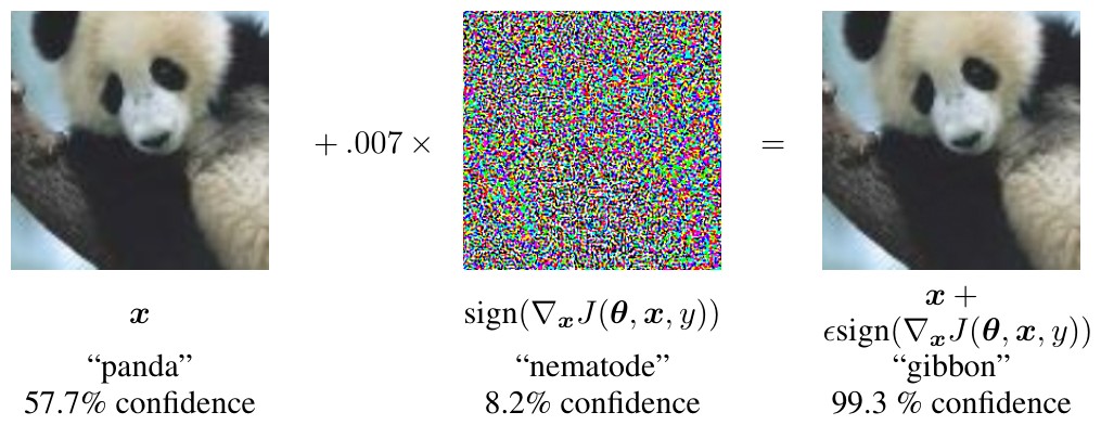
“panda”		“nematode”		“gibbon”
57.7% confidence		8.2% confidence		99.3 % confidence

Figure 1: A demonstration of fast adversarial example generation applied to GoogLeNet (Szegedy et al., 2014a) on ImageNet. By adding an imperceptibly small vector whose elements are equal to the sign of the elements of the gradient of the cost function with respect to the input, we can change GoogLeNet’s classification of the image. Here our ${\epsilon}$ of .007 corresponds to the magnitude of the smallest bit of an 8 bit image encoding after GoogLeNet’s conversion to real numbers.

图 1：把快速对抗样本生成应用到 ImageNet 上的 GoogLeNet (Szegedy 等人, 2014a) 的一次演示。加上一个不可察觉的小向量，其元素等于代价函数对输入的梯度各元素的符号，我们就能改变 GoogLeNet 对这张图的分类。这里我们取的 ${\epsilon}$ 为 .007，对应的是 8 比特图像编码在 GoogLeNet 把它转换成实数之后的最低有效位的幅度。

5 Adversarial training of linear models versus weight decay

5 线性模型的对抗训练与权重衰减

Perhaps the simplest possible model we can consider is logistic regression. In this case, the fast gradient sign method is exact. We can use this case to gain some intuition for how adversarial examples are generated in a simple setting. See Fig. 2 for instructive images.

我们能考虑的最简单模型，大概就是逻辑回归。在这种情形下，快速梯度符号法是精确的。我们可以用它来获得一些直觉，看看在简单设定里对抗样本是怎样生成的。见图 2 中便于说明的图像。

If we train a single model to recognize labels $y\in\{-1,1\}$ with $P(y=1)=\sigma\left({\bm{w}}^{\top}{\bm{x}}+b\right)$ where $\sigma(z)$ is the logistic sigmoid function, then training consists of gradient descent on

如果我们训练单个模型来识别标签 $y\in\{-1,1\}$，并取 $P(y=1)=\sigma\left({\bm{w}}^{\top}{\bm{x}}+b\right)$，其中 $\sigma(z)$ 是 logistic sigmoid 函数，那么训练就是对下式做梯度下降

$$\mathbb{E}_{{\bm{x}},y\sim p_{\text{data}}}\zeta(-y({\bm{w}}^{\top}{\bm{x}}+b))$$

where $\zeta(z)=\log\left(1+\exp(z)\right)$ is the softplus function. We can derive a simple analytical form for training on the worst-case adversarial perturbation of ${\bm{x}}$ rather than ${\bm{x}}$ itself, based on gradient sign perturbation. Note that the sign of the gradient is just $-{\text{sign}}({\bm{w}})$, and that ${\bm{w}}^{\top}{\text{sign}}({\bm{w}})=||{\bm{w}}||_{1}$. The adversarial version of logistic regression is therefore to minimize

其中 $\zeta(z)=\log\left(1+\exp(z)\right)$ 是 softplus 函数。基于梯度符号扰动，我们可以推导出一个简单的解析形式，用来在 ${\bm{x}}$ 的最坏情况对抗扰动上训练，而不是在 ${\bm{x}}$ 本身上训练。注意，梯度的符号恰好是 $-{\text{sign}}({\bm{w}})$，并且 ${\bm{w}}^{\top}{\text{sign}}({\bm{w}})=||{\bm{w}}||_{1}$。因此，逻辑回归的对抗版本就是最小化

$$\mathbb{E}_{{\bm{x}},y\sim p_{\text{data}}}\zeta(y({\epsilon}||{\bm{w}}||_{1}-{\bm{w}}^{\top}{\bm{x}}-b)).$$

This is somewhat similar to $L^{1}$ regularization. However, there are some important differences. Most significantly, the $L^{1}$ penalty is subtracted off the model’s activation during training, rather than added to the training cost. This means that the penalty can eventually start to disappear if the model learns to make confident enough predictions that $\zeta$ saturates. This is not guaranteed to happen—in the underfitting regime, adversarial training will simply worsen underfitting. We can thus view $L^{1}$ weight decay as being more “worst case” than adversarial training, because it fails to deactivate in the case of good margin.

这与 $L^{1}$ 正则有些相似。不过有几处重要差别。最显著的是，$L^{1}$ 惩罚在训练时是从模型的激活里减掉的，而不是加到训练代价上。这意味着，如果模型学会做出足够自信的预测、使 $\zeta$ 进入饱和，这份惩罚最终可能开始消失。这并不是一定会发生的——在欠拟合区间，对抗训练只会让欠拟合更严重。因此我们可以把 $L^{1}$ 权重衰减看成比对抗训练更“最坏情况”，因为它在间隔已经足够好的时候不会停下来。

If we move beyond logistic regression to multiclass softmax regression, $L^{1}$ weight decay becomes even more pessimistic, because it treats each of the softmax’s outputs as independently perturbable, when in fact it is usually not possible to find a single ${\bm{\eta}}$ that aligns with all of the class’s weight vectors. Weight decay overestimates the damage achievable with perturbation even more in the case of a deep network with multiple hidden units. Because $L^{1}$ weight decay overestimates the amount of damage an adversary can do, it is necessary to use a smaller $L^{1}$ weight decay coefficient than the ${\epsilon}$ associated with the precision of our features. When training maxout networks on MNIST, we obtained good results using adversarial training with ${\epsilon}=.25$. When applying $L^{1}$ weight decay to the first layer, we found that even a coefficient of .0025 was too large, and caused the model to get stuck with over 5% error on the training set. Smaller weight decay coefficients permitted succesful training but conferred no regularization benefit.

如果从逻辑回归走到多类 softmax 回归，$L^{1}$ 权重衰减会变得更加悲观，因为它把 softmax 的每一个输出都当成可以独立扰动的，而实际上通常找不到一个能与所有类别权重向量都对齐的单一 ${\bm{\eta}}$。在有多个隐单元的深度网络里，权重衰减对扰动所能造成伤害的高估还要更严重。正因为 $L^{1}$ 权重衰减高估了对手能造成的伤害，就必须使用比与特征精度相对应的 ${\epsilon}$ 更小的 $L^{1}$ 权重衰减系数。在 MNIST 上训练 maxout 网络时，我们用 ${\epsilon}=.25$ 的对抗训练得到了好结果。把 $L^{1}$ 权重衰减加到第一层时，我们发现即便系数取 .0025 也太大了，会让模型卡在训练集误差超过 5% 的地方。更小的权重衰减系数能够让训练成功进行，但没有带来正则收益。

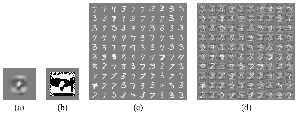
(a)	(b)	(c)	(d)

Figure 2: The fast gradient sign method applied to logistic regression (where it is not an approximation, but truly the most damaging adversarial example in the max norm box). a) The weights of a logistic regression model trained on MNIST. b) The sign of the weights of a logistic regression model trained on MNIST. This is the optimal perturbation. Even though the model has low capacity and is fit well, this perturbation is not readily recognizable to a human observer as having anything to do with the relationship between 3s and 7s. c) MNIST 3s and 7s. The logistic regression model has a 1.6% error rate on the 3 versus 7 discrimination task on these examples. d) Fast gradient sign adversarial examples for the logistic regression model with ${\epsilon}=.25$. The logistic regression model has an error rate of 99% on these examples.

图 2：把快速梯度符号法用在逻辑回归上（在这里它不是近似，而确实是最大范数盒子里最具破坏性的对抗样本）。a) 在 MNIST 上训练的逻辑回归模型的权重。b) 在 MNIST 上训练的逻辑回归模型权重的符号。这就是最优扰动。尽管模型容量很低、也拟合得很好，这一扰动在人类观察者看来，并不容易认出与 3 和 7 之间的关系有什么相干之处。c) MNIST 中的 3 和 7。逻辑回归模型在这些例子上做 3 对 7 的判别，误差率为 1.6%。d) 取 ${\epsilon}=.25$ 时，该逻辑回归模型的快速梯度符号对抗样本。逻辑回归模型在这些例子上的误差率为 99%。

6 Adversarial training of deep networks

6 深度网络的对抗训练

The criticism of deep networks as vulnerable to adversarial examples is somewhat misguided, because unlike shallow linear models, deep networks are at least able to represent functions that resist adversarial perturbation. The universal approximator theorem (Hornik et al., 1989) guarantees that a neural network with at least one hidden layer can represent any function to an arbitary degree of accuracy so long as its hidden layer is permitted to have enough units. Shallow linear models are not able to become constant near training points while also assigning different outputs to different training points.

批评深度网络容易受到对抗样本攻击，其实有些偏了，因为与浅层线性模型不同，深度网络至少有能力 表示 能够抵抗对抗扰动的函数。万能逼近定理 (Hornik 等人, 1989) 保证：只要允许隐层有足够多的单元，至少有一层隐层的神经网络可以把任意函数表示到任意精度。浅层线性模型做不到在训练点附近变成常数的同时，又给不同训练点赋上不同的输出。

Of course, the universal approximator theorem does not say anything about whether a training algorithm will be able to discover a function with all of the desired properties. Obviously, standard supervised training does not specify that the chosen function be resistant to adversarial examples. This must be encoded in the training procedure somehow.

当然，万能逼近定理并没有说训练算法是否能够发现一个具备全部所需性质的函数。很明显，标准的监督训练并没有规定所选函数必须抵抗对抗样本。这一点必须以某种方式写进训练过程里。

Szegedy et al. (2014b) showed that by training on a mixture of adversarial and clean examples, a neural network could be regularized somewhat. Training on adversarial examples is somewhat different from other data augmentation schemes; usually, one augments the data with transformations such as translations that are expected to actually occur in the test set. This form of data augmentation instead uses inputs that are unlikely to occur naturally but that expose flaws in the ways that the model conceptualizes its decision function. At the time, this procedure was never demonstrated to improve beyond dropout on a state of the art benchmark. However, this was partially because it was difficult to experiment extensively with expensive adversarial examples based on L-BFGS.

Szegedy 等人 (2014b) 表明，在对抗样本与干净样本的混合上训练，可以对神经网络起到一定的正则作用。在对抗样本上训练，与其他数据增广方案有些不同：通常人们会用平移这类预期在测试集上也会真实出现的变换来增广数据。这种数据增广用的却是不太可能自然出现、但能暴露模型对其决策函数概念化方式中缺陷的输入。在当时，这一做法从未被证明能在前沿基准上超过 dropout。不过，这部分是因为基于 L-BFGS 的对抗样本太贵，很难做大量实验。

We found that training with an adversarial objective function based on the fast gradient sign method was an effective regularizer:

我们发现，用基于快速梯度符号法的对抗目标函数来训练，是一种有效的正则：

$$\tilde{J}({\bm{\theta}},{\bm{x}},y)=\alpha J({\bm{\theta}},{\bm{x}},y)+(1-\alpha)J({\bm{\theta}},{\bm{x}}+{\epsilon}{\text{sign}}\left(\nabla_{\bm{x}}J({\bm{\theta}},{\bm{x}},y)\right).$$

In all of our experiments, we used $\alpha=0.5$. Other values may work better; our initial guess of this hyperparameter worked well enough that we did not feel the need to explore more. This approach means that we continually update our supply of adversarial examples, to make them resist the current version of the model. Using this approach to train a maxout network that was also regularized with dropout, we were able to reduce the error rate from 0.94% without adversarial training to 0.84% with adversarial training.

在我们的全部实验中，都取 $\alpha=0.5$。其他取值或许更好；我们对这一超参数的最初猜测已经足够好，因而没有觉得有必要再多探索。这一做法意味着，我们会不断更新手头的对抗样本，使它们能够抵抗模型的当前版本。用这种方法训练一个同时也用 dropout 正则的 maxout 网络，我们把误差率从没有对抗训练时的 0.94%，降到了有对抗训练时的 0.84%。

We observed that we were not reaching zero error rate on adversarial examples on the training set. We fixed this problem by making two changes. First, we made the model larger, using 1600 units per layer rather than the 240 used by the original maxout network for this problem. Without adversarial training, this causes the model to overfit slightly, and get an error rate of 1.14% on the test set. With adversarial training, we found that the validation set error leveled off over time, and made very slow progress. The original maxout result uses early stopping, and terminates learning after the validation set error rate has not decreased for 100 epochs. We found that while the validation set error was very flat, the adversarial validation set error was not. We therefore used early stopping on the adversarial validation set error. Using this criterion to choose the number of epochs to train for, we then retrained on all 60,000 examples. Five different training runs using different seeds for the random number generators used to select minibatches of training examples, initialize model weights, and generate dropout masks result in four trials that each had an error rate of 0.77% on the test set and one trial that had an error rate of 0.83%. The average of 0.782% is the best result reported on the permutation invariant version of MNIST, though statistically indistinguishable from the result obtained by fine-tuning DBMs with dropout (Srivastava et al., 2014) at 0.79%.

我们观察到，训练集上的对抗样本误差率并没有降到零。我们做了两处修改来解决这个问题。第一，把模型加大，每层使用 1600 个单元，而不是原版 maxout 网络在这个问题上所用的 240 个。若不做对抗训练，这会让模型略微过拟合，测试集误差率为 1.14%。做了对抗训练之后，我们发现验证集误差会随时间趋于平稳，进展非常缓慢。原来的 maxout 结果使用早停，在验证集误差率连续 100 个 epoch 不再下降后结束学习。我们发现，尽管验证集误差非常平坦，对抗 验证集误差却并非如此。因此我们改用 对抗验证集误差 来做早停。用这一标准选定训练的 epoch 数后，再在全部 60,000 个例子上重新训练。五次不同的训练运行使用了不同的随机数种子，分别用于选取训练样本的 minibatch、初始化模型权重、以及生成 dropout 掩码，结果有四次试验的测试集误差率都是 0.77%，另一次是 0.83%。平均 0.782% 是在排列不变版本的 MNIST 上报告过的最好结果，不过在统计上与用 dropout 微调 DBM (Srivastava 等人, 2014) 得到的 0.79% 无法区分。

The model also became somewhat resistant to adversarial examples. Recall that without adversarial training, this same kind of model had an error rate of 89.4% on adversarial examples based on the fast gradient sign method. With adversarial training, the error rate fell to 17.9%. Adversarial examples are transferable between the two models but with the adversarially trained model showing greater robustness. Adversarial examples generated via the original model yield an error rate of 19.6% on the adversarially trained model, while adversarial examples generated via the new model yield an error rate of 40.9% on the original model. When the adversarially trained model does misclassify an adversarial example, its predictions are unfortunately still highly confident. The average confidence on a misclassified example was 81.4%. We also found that the weights of the learned model changed significantly, with the weights of the adversarially trained model being significantly more localized and interpretable (see Fig. 3).

模型对对抗样本也变得有些抵抗力。请回忆，在不做对抗训练时，同一类模型在基于快速梯度符号法的对抗样本上误差率是 89.4%。做了对抗训练之后，误差率降到 17.9%。对抗样本可以在这两个模型之间迁移，但经过对抗训练的模型表现出更强的稳健性。用原模型生成的对抗样本，在对抗训练模型上的误差率是 19.6%；用新模型生成的对抗样本，在原模型上的误差率是 40.9%。当对抗训练模型确实把一个对抗样本分错时，它的预测仍然把握很高，这一点并不令人乐观。分错例子上的平均把握是 81.4%。我们还发现，学到的模型权重发生了显著变化：经过对抗训练的模型，其权重明显更加局部、也更好解释（见图 3）。

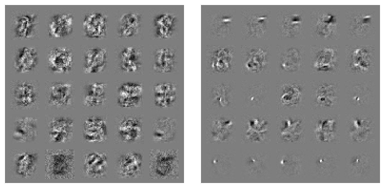
Figure 3: Weight visualizations of maxout networks trained on MNIST. Each row shows the filters for a single maxout unit. Left) Naively trained model. Right) Model with adversarial training.

图 3：在 MNIST 上训练的 maxout 网络的权重可视化。每一行展示单个 maxout 单元的滤波器。左）朴素训练的模型。右）经过对抗训练的模型。

The adversarial training procedure can be seen as minimizing the worst case error when the data is perturbed by an adversary. That can be interpreted as learning to play an adversarial game, or as minimizing an upper bound on the expected cost over noisy samples with noise from $U(-{\epsilon},{\epsilon})$ added to the inputs. Adversarial training can also be seen as a form of active learning, where the model is able to request labels on new points. In this case the human labeler is replaced with a heuristic labeler that copies labels from nearby points.

对抗训练过程可以看成：在数据被对手扰动时，最小化最坏情况误差。这可以解释成学习去玩一场对抗博弈，也可以解释成在输入上加上来自 $U(-{\epsilon},{\epsilon})$ 的噪声后，最小化噪声样本上期望代价的一个上界。对抗训练还可以看成一种主动学习，模型能够在新的点上请求标签。这时，人类标注者被一个启发式标注者取代，后者把附近点的标签复制过来。

We could also regularize the model to be insensitive to changes in its features that are smaller than the ${\epsilon}$ precision simply by training on all points within the ${\epsilon}$ max norm box, or sampling many points within this box. This corresponds to adding noise with max norm ${\epsilon}$ during training. However, noise with zero mean and zero covariance is very inefficient at preventing adversarial examples. The expected dot product between any reference vector and such a noise vector is zero. This means that in many cases the noise will have essentially no effect rather than yielding a more difficult input. In fact, in many cases the noise will actualy result in a lower objective function value. We can think of adversarial training as doing hard example mining among the set of noisy inputs, in order to train more efficiently by considering only those noisy points that strongly resist classification. As control experiments, we trained training a maxout network with noise based on randomly adding $\pm{\epsilon}$ to each pixel, or adding noise in $U(-{\epsilon},{\epsilon})$ to each pixel. These obtained an error rate of 86.2% with confidence 97.3% and an error rate of 90.4% with a confidence of 97.8% respectively on fast gradient sign adversarial examples.

我们也可以让模型对小于 ${\epsilon}$ 精度的特征变化不敏感，办法很简单：在 ${\epsilon}$ 最大范数盒子里的所有点上训练，或在这个盒子里采样许多点。这对应于训练时加上最大范数为 ${\epsilon}$ 的噪声。不过，均值为零、协方差为零的噪声，在防止对抗样本方面效率很低。任意参考向量与这种噪声向量的期望点积都是零。这意味着，在许多情形下，噪声本质上不会产生任何效果，而不会给出更难的输入。事实上，在许多情形下，噪声实际上还会让目标函数值变得更低。我们可以把对抗训练看成在噪声输入集合里做困难样本挖掘，从而只考虑那些强烈抵抗分类的噪声点，以便更高效地训练。作为对照实验，我们训练过一个 maxout 网络，噪声是随机给每个像素加上 $\pm{\epsilon}$，或给每个像素加上 $U(-{\epsilon},{\epsilon})$ 中的噪声。它们在快速梯度符号对抗样本上的误差率分别是 86.2%（把握 97.3%）和 90.4%（把握 97.8%）。

Because the derivative of the sign function is zero or undefined everywhere, gradient descent on the adversarial objective function based on the fast gradient sign method does not allow the model to anticipate how the adversary will react to changes in the parameters. If we instead adversarial examples based on small rotations or addition of the scaled gradient, then the perturbation process is itself differentiable and the learning can take the reaction of the adversary into account. However, we did not find nearly as powerful of a regularizing result from this process, perhaps because these kinds of adversarial examples are not as difficult to solve.

由于符号函数的导数处处为零或没有定义，基于快速梯度符号法的对抗目标函数上的梯度下降，并不能让模型预见到对手会如何对参数变化作出反应。如果我们改为基于小角度旋转或加上缩放后的梯度来构造对抗样本，那么扰动过程本身就是可微的，学习就可以把对手的反应考虑进去。不过，我们并没有发现这一过程能带来同样强的正则效果，或许是因为这类对抗样本没有那么难解决。

One natural question is whether it is better to perturb the input or the hidden layers or both. Here the results are inconsistent. Szegedy et al. (2014b) reported that adversarial perturbations yield the best regularization when applied to the hidden layers. That result was obtained on a sigmoidal network. In our experiments with the fast gradient sign method, we find that networks with hidden units whose activations are unbounded simply respond by making their hidden unit activations very large, so it is usually better to just perturb the original input. On saturating models such as the Rust model we found that perturbation of the input performed comparably to perturbation of the hidden layers. Perturbations based on rotating the hidden layers solve the problem of unbounded activations growing to make additive perturbations smaller by comparison. We were able to succesfully train maxout networks with rotational perturbations of the hidden layers. However, this did not yield nearly as strong of a regularizing effect as additive perturbation of the input layer. Our view of adversarial training is that it is only clearly useful when the model has the capacity to learn to resist adversarial examples. This is only clearly the case when a universal approximator theorem applies. Because the last layer of a neural network, the linear-sigmoid or linear-softmax layer, is not a universal approximator of functions of the final hidden layer, this suggests that one is likely to encounter problems with underfitting when applying adversarial perturbations to the final hidden layer. We indeed found this effect. Our best results with training using perturbations of hidden layers never involved perturbations of the final hidden layer.

一个自然的问题是：扰动输入更好，还是扰动隐层更好，还是两者都扰动更好。这里的结果并不一致。Szegedy 等人 (2014b) 报告说，把对抗扰动加在隐层上，正则效果最好。那一结果是在 sigmoid 网络上得到的。在我们用快速梯度符号法做的实验中，我们发现，激活无界的隐单元网络只会把隐单元激活变得非常大，因此通常只扰动原始输入会更好。在像 Rust 模型这样的饱和模型上，我们发现扰动输入与扰动隐层的效果相当。基于旋转隐层的扰动，可以解决无界激活变大、从而使加性扰动相对变小的问题。我们成功地用隐层的旋转扰动训练了 maxout 网络。不过，这并没有带来与在输入层做加性扰动几乎同样强的正则效果。我们对对抗训练的看法是：只有当模型有容量去学习抵抗对抗样本时，它的用处才是清楚的。而这一点只有在万能逼近定理适用时才清楚成立。因为神经网络的最后一层，也就是线性-sigmoid 或线性-softmax 层，并不是最终隐层上函数的万能逼近器，这就提示：把对抗扰动加到最后一层隐层上，很可能会遇到欠拟合。我们的确发现了这一效应。我们在隐层扰动上得到的最好结果，从未包含对最后一层隐层的扰动。

7 Different kinds of model capacity

7 不同种类的模型容量

One reason that the existence of adversarial examples can seem counter-intuitive is that most of us have poor intuitions for high dimensional spaces. We live in three dimensions, so we are not used to small effects in hundreds of dimensions adding up to create a large effect. There is another way that our intuitions serve us poorly. Many people think of models with low capacity as being unable to make many different confident predictions. This is not correct. Some models with low capacity do exhibit this behavior. For example shallow RBF networks with

对抗样本的存在看起来会有违直觉，原因之一是我们大多数人对高维空间的直觉都很差。我们生活在三维里，因而不习惯数百个维度上的微小效应加在一起，变成一次很大的效果。还有另一种方式让我们的直觉帮了倒忙。许多人认为，容量低的模型无法做出许多不同的、有把握的预测。这并不正确。有些低容量模型的确表现出这种行为。例如，浅层 RBF 网络采用

$$p(y=1\mid{\bm{x}})=\exp\left(({\bm{x}}-\mu)^{\top}{\bm{\beta}}({\bm{x}}-\mu)\right)$$

are only able to confidently predict that the positive class is present in the vicinity of $\mu$. Elsewhere, they default to predicting the class is absent, or have low-confidence predictions.

它们只能在 $\mu$ 附近有把握地预测正类存在。在其他地方，它们会默认预测该类不存在，或者给出低把握的预测。

RBF networks are naturally immune to adversarial examples, in the sense that they have low confidence when they are fooled. A shallow RBF network with no hidden layers gets an error rate of 55.4% on MNIST using adversarial examples generated with the fast gradient sign method and ${\epsilon}=.25$. However, its confidence on mistaken examples is only $1.2\%$. Its average confidence on clean test examples is $60.6$%. We can’t expect a model with such low capacity to get the right answer at all points of space, but it does correctly respond by reducing its confidence considerably on points it does not “understand.”

RBF 网络对对抗样本有一种天然的免疫，意思是：被骗的时候，它们的把握很低。一个没有隐层的浅层 RBF 网络，在用快速梯度符号法、取 ${\epsilon}=.25$ 生成的对抗样本上，MNIST 误差率为 55.4%。不过，它在分错例子上的把握只有 $1.2\%$。它在干净测试例子上的平均把握是 $60.6$%。我们不能指望一个容量如此低的模型在空间中所有点上都给出正确答案，但它确实会在自己并不“理解”的点上，正确地大幅降低把握。

RBF units are unfortunately not invariant to any significant transformations so they cannot generalize very well. We can view linear units and RBF units as different points on a precision-recall tradeoff curve. Linear units achieve high recall by responding to every input in a certain direction, but may have low precision due to responding too strongly in unfamiliar situations. RBF units achieve high precision by responding only to a specific point in space, but in doing so sacrifice recall. Motivated by this idea, we decided to explore a variety of models involving quadratic units, including deep RBF networks. We found this to be a difficult task—very model with sufficient quadratic inhibition to resist adversarial perturbation obtained high training set error when trained with SGD.

遗憾的是，RBF 单元对任何显著的变换都没有不变性，因此泛化能力不太好。我们可以把线性单元和 RBF 单元看成精确率-召回率权衡曲线上的不同位置。线性单元会对某个方向上的每一个输入都作出响应，因而召回率高，但在不熟悉的情形下响应过强，精确率可能就低。RBF 单元只对空间中一个特定的点作出响应，因而精确率高，但这样做牺牲了召回率。受这一想法推动，我们决定探索各种包含二次单元的模型，包括深层 RBF 网络。我们发现这是一项困难的任务——凡是二次抑制强到足以抵抗对抗扰动的模型，用 SGD 训练时，训练集误差都会很高。

8 Why do adversarial examples generalize?

8 对抗样本为何会泛化？

An intriguing aspect of adversarial examples is that an example generated for one model is often misclassified by other models, even when they have different architecures or were trained on disjoint training sets. Moreover, when these different models misclassify an adversarial example, they often agree with each other on its class. Explanations based on extreme non-linearity and overfitting cannot readily account for this behavior—why should multiple extremely non-linear model with excess capacity consistently label out-of-distribution points in the same way? This behavior is especially surprising from the view of the hypothesis that adversarial examples finely tile space like the rational numbers among the reals, because in this view adversarial examples are common but occur only at very precise locations.

对抗样本一个引人注目的方面是：为某个模型生成的例子，常常也会被其他模型分错，即便它们的结构不同，或者是在互不相交的训练集上训练的。不仅如此，当这些不同模型把一个对抗样本分错时，它们往往还会在其类别上彼此一致。基于极端非线性和过拟合的解释，不太容易说明这种行为——为什么多个容量过剩、又极端非线性的模型，会一致地给分布外的点标上同一类？若从“对抗样本像有理数嵌在实数中那样细密地铺满空间”这一假说看来，这种行为尤其令人吃惊，因为按那种看法，对抗样本虽然常见，却只出现在非常精确的位置上。

Under the linear view, adversarial examples occur in broad subspaces. The direction ${\bm{\eta}}$ need only have positive dot product with the gradient of the cost function, and ${\epsilon}$ need only be large enough. Fig. 4 demonstrates this phenomenon. By tracing out different values of ${\epsilon}$ we see that adversarial examples occur in contiguous regions of the 1-D subspace defined by the fast gradient sign method, not in fine pockets. This explains why adversarial examples are abundant and why an example misclassified by one classifier has a fairly high prior probability of being misclassified by another classifier.

在线性观点下，对抗样本出现在很宽的子空间里。方向 ${\bm{\eta}}$ 只需与代价函数的梯度有正的点积，${\epsilon}$ 只需足够大。图 4 展示了这一现象。通过追踪不同的 ${\epsilon}$ 取值，我们看到对抗样本出现在快速梯度符号法所定义的一维子空间的连续区域里，而不是细小的口袋中。这就解释了为何对抗样本大量存在，以及为何被一个分类器分错的例子，有相当高的先验概率也会被另一个分类器分错。

To explain why mutiple classifiers assign the same class to adversarial examples, we hypothesize that neural networks trained with current methodologies all resemble the linear classifier learned on the same training set. This reference classifier is able to learn approximately the same classification weights when trained on different subsets of the training set, simply because machine learning algorithms are able to generalize. The stability of the underlying classification weights in turn results in the stability of adversarial examples.

至于为何多个分类器会给对抗样本赋上 同一个类别，我们的假说是：用当前方法训练出来的神经网络，都类似于在同一训练集上学到的线性分类器。这个参照分类器在训练集的不同子集上训练时，能够学到大致相同的分类权重，只不过是因为机器学习算法能够泛化。底层分类权重的稳定性，反过来又造成了对抗样本的稳定性。

To test this hypothesis, we generated adversarial examples on a deep maxout network and classified these examples using a shallow softmax network and a shallow RBF network. On examples that were misclassified by the maxout network, the RBF network predicted the maxout network’s class assignment only 16.0% of the time, while the softmax classifier predict the maxout network’s class correctly 54.6% of the time. These numbers are largely driven by the differing error rate of the different models though. If we exclude our attention to cases where both models being compared make a mistake, then softmax regression predict’s maxout’s class 84.6% of the time, while the RBF network is able to predict maxout’s class only 54.3% of the time. For comparison, the RBF network can predict softmax regression’s class 53.6% of the time, so it does have a strong linear component to its own behavior. Our hypothesis does not explain all of the maxout network’s mistakes or all of the mistakes that generalize across models, but clearly a significant proportion of them are consistent with linear behavior being a major cause of cross-model generalization.

为了检验这一假说，我们在一个深度 maxout 网络上生成对抗样本，再用一个浅层 softmax 网络和一个浅层 RBF 网络来分类这些例子。在被 maxout 网络分错的例子上，RBF 网络只有 16.0% 的时候预测出 maxout 网络所赋的类别，而 softmax 分类器有 54.6% 的时候正确预测出 maxout 网络的类别。不过这些数字在很大程度上是由不同模型不同的误差率驱动的。如果把注意力限制在两个被比较的模型都分错的情形，那么 softmax 回归有 84.6% 的时候预测出 maxout 的类别，而 RBF 网络只有 54.3% 的时候能够预测出 maxout 的类别。作为对照，RBF 网络有 53.6% 的时候能够预测出 softmax 回归的类别，因此它自身的行为里也有很强的线性成分。我们的假说并不能解释 maxout 网络的全部错误，也不能解释全部在模型之间泛化的错误，但显然有相当一部分与“线性行为是跨模型泛化的主要原因”这一点相符。

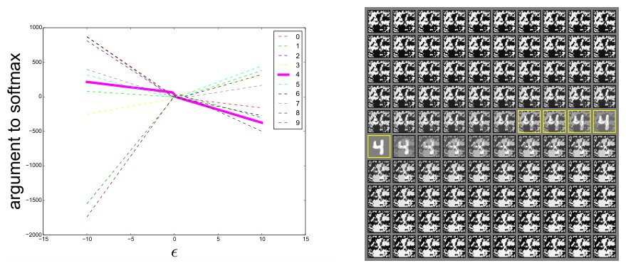
Figure 4: By tracing out different values of ${\epsilon}$, we can see that adversarial examples occur reliably for almost any sufficiently large value of ${\epsilon}$ provided that we move in the correct direction. Correct classifications occur only on a thin manifold where ${\bm{x}}$ occurs in the data. Most of $\mathbb{R}^{n}$ consists of adversarial examples and rubbish class examples (see the appendix). This plot was made from a naively trained maxout network. Left) A plot showing the argument to the softmax layer for each of the 10 MNIST classes as we vary ${\epsilon}$ on a single input example. The correct class is 4. We see that the unnormalized log probabilities for each class are conspicuously piecewise linear with ${\epsilon}$ and that the wrong classifications are stable across a wide region of ${\epsilon}$ values. Moreover, the predictions become very extreme as we increase ${\epsilon}$ enough to move into the regime of rubbish inputs. Right) The inputs used to generate the curve (upper left = negative ${\epsilon}$, lower right = positive ${\epsilon}$, yellow boxes indicate correctly classified inputs).

图 4：通过追踪不同的 ${\epsilon}$ 取值，可以看到：只要沿着正确方向移动，对几乎任何足够大的 ${\epsilon}$，对抗样本都会稳定出现。正确分类只发生在数据中 ${\bm{x}}$ 所在的那条很薄的流形上。$\mathbb{R}^{n}$ 的大部分由对抗样本和 垃圾类样本 组成（见附录）。本图来自一个朴素训练的 maxout 网络。左）在单个输入例子上改变 ${\epsilon}$ 时，10 个 MNIST 类别各自进入 softmax 层的自变量。正确类别是 4。可以看到，每个类别未经归一化的对数概率对 ${\epsilon}$ 明显是分段线性的，而且错误分类在很宽的 ${\epsilon}$ 取值区间里都保持稳定。此外，当把 ${\epsilon}$ 加大到进入垃圾输入区间时，预测会变得非常极端。右）用来生成这条曲线的输入（左上为负的 ${\epsilon}$，右下为正的 ${\epsilon}$，黄框标出被正确分类的输入）。

9 Alternative hypotheses

9 其他假说

We now consider and refute some alternative hypotheses for the existence of adversarial examples. First, one hypothesis is that generative training could provide more constraint on the training process, or cause the model to learn what to distinguish “real” from “fake” data and be confident only on “real” data. The MP-DBM (Goodfellow et al., 2013a) provides a good model to test this hypothesis. Its inference procedure gets good classification accuracy (an 0.88% error rate) on MNIST. This inference procedure is differentiable. Other generative models either have non-differentiable inference procedures, making it harder to compute adversarial examples, or require an additional non-generative discriminator model to get good classification accuracy on MNIST. In the case of the MP-DBM, we can be sure that the generative model itself is responding to adversarial examples, rather than the non-generative classifier model on top. We find that the model is vulnerable to adversarial examples. With an $\epsilon$ of 0.25, we find an error rate of 97.5% on adversarial examples generated from the MNIST test set. It remains possible that some other form of generative training could confer resistance, but clearly the mere fact of being generative is not alone sufficient.

我们现在考虑并反驳关于对抗样本存在的一些其他假说。首先，一种假说是：生成式训练能够给训练过程提供更多约束，或者让模型学会区分“真”数据和“假”数据，并且只在“真”数据上保持自信。MP-DBM (Goodfellow 等人, 2013a) 是检验这一假说的好模型。它的推断过程在 MNIST 上能得到很好的分类精度（误差率 0.88%）。这一推断过程是可微的。其他生成模型要么推断过程不可微，从而更难计算对抗样本，要么需要再加一个非生成的判别模型，才能在 MNIST 上得到好的分类精度。就 MP-DBM 而言，我们可以确定是生成模型本身在对对抗样本作出反应，而不是上面那个非生成的分类器模型。我们发现，该模型容易受到对抗样本的攻击。取 $\epsilon$ 为 0.25 时，在由 MNIST 测试集生成的对抗样本上，误差率为 97.5%。仍然有可能，某种其他形式的生成式训练能够带来抵抗力，但很清楚，仅仅“是生成式的”这一点本身并不足够。

Another hypothesis about why adversarial examples exist is that individual models have strange quirks but averaging over many models can cause adversarial examples to wash out. To test this hypothesis, we trained an ensemble of twelve maxout networks on MNIST. Each network was trained using a different seed for the random number generator used to initialize the weights, generate dropout masks, and select minibatches of data for stochastic gradient descent. The ensemble gets an error rate of 91.1% on adversarial examples designed to perturb the entire ensemble with $\epsilon=.25$. If we instead use adversarial examples designed to perturb only one member of the ensemble, the error rate falls to 87.9%. Ensembling provides only limited resistance to adversarial perturbation.

关于对抗样本为何存在的另一种假说是：单个模型会有奇怪的癖性，但在许多模型上取平均，就能把对抗样本冲淡。为了检验这一假说，我们在 MNIST 上训练了十二个 maxout 网络的集成。每个网络使用不同的随机数种子来初始化权重、生成 dropout 掩码，以及选取随机梯度下降所用的数据 minibatch。该集成对设计来扰动整个集成、且 $\epsilon=.25$ 的对抗样本，误差率为 91.1%。如果改为使用只扰动集成中某一个成员的对抗样本，误差率降到 87.9%。集成对对抗扰动只提供了有限的抵抗力。

10 Summary and discussion

10 小结与讨论

As a summary, this paper has made the following observations:

作为小结，本文做出了以下观察：

• • Adversarial examples can be explained as a property of high-dimensional dot products. They are a result of models being too linear, rather than too nonlinear.

• 对抗样本可以解释成高维点积的一种性质。它们是模型过于线性的结果，而不是过于非线性的结果。

• • The generalization of adversarial examples across different models can be explained as a result of adversarial perturbations being highly aligned with the weight vectors of a model, and different models learning similar functions when trained to perform the same task.

• 对抗样本在不同模型之间的泛化，可以解释为：对抗扰动与模型的权重向量高度对齐，而不同模型在被训练去做同一任务时会学到相似的函数。

• • The direction of perturbation, rather than the specific point in space, matters most. Space is not full of pockets of adversarial examples that finely tile the reals like the rational numbers.

• 最要紧的是扰动的方向，而不是空间中那个特定的点。空间并没有布满像有理数细密铺在实数中那样的对抗样本口袋。

• • Because it is the direction that matters most, adversarial perturbations generalize across different clean examples.

• 正因为方向最要紧，对抗扰动才会在不同的干净例子之间泛化。

• • We have introduced a family of fast methods for generating adversarial examples.

• 我们引入了一族快速生成对抗样本的方法。

• • We have demonstrated that adversarial training can result in regularization; even further regularization than dropout.

• 我们表明，对抗训练可以带来正则效果；甚至比 dropout 还要多一截正则。

• • We have run control experiments that failed to reproduce this effect with simpler but less efficient regularizers including $L^{1}$ weight decay and adding noise.

• 我们做了对照实验，用 $L^{1}$ 权重衰减和加噪声这类更简单、但效率更低的正则，没能复现这一效果。

• • Models that are easy to optimize are easy to perturb.

• 容易优化的模型，也容易被扰动。

• • Linear models lack the capacity to resist adversarial perturbation; only structures with a hidden layer (where the universal approximator theorem applies) should be trained to resist adversarial perturbation.

• 线性模型没有抵抗对抗扰动的容量；只有带隐层的结构（万能逼近定理在那里适用）才应当被训练去抵抗对抗扰动。

• • RBF networks are resistant to adversarial examples.

• RBF 网络能够抵抗对抗样本。

• • Models trained to model the input distribution are not resistant to adversarial examples.

• 被训练去建模输入分布的模型，并不能抵抗对抗样本。

• • Ensembles are not resistant to adversarial examples.

• 集成并不能抵抗对抗样本。

Some further observations concerning rubbish class examples are presented in the appendix:

附录中还给出了一些关于 垃圾类样本 的进一步观察：

• • Rubbish class examples are ubiquitous and easily generated.

• 垃圾类样本无处不在，也很容易生成。

• • Shallow linear models are not resistant to rubbish class examples.

• 浅层线性模型并不能抵抗垃圾类样本。

• • RBF networks are resistant to rubbish class examples.

• RBF 网络能够抵抗垃圾类样本。

Gradient-based optimization is the workhorse of modern AI. Using a network that has been designed to be sufficiently linear–whether it is a ReLU or maxout network, an LSTM, or a sigmoid network that has been carefully configured not to saturate too much– we are able to fit most problems we care about, at least on the training set. The existence of adversarial examples suggests that being able to explain the training data or even being able to correctly label the test data does not imply that our models truly understand the tasks we have asked them to perform. Instead, their linear responses are overly confident at points that do not occur in the data distribution, and these confident predictions are often highly incorrect. This work has shown we can partially correct for this problem by explicitly identifying problematic points and correcting the model at each of these points. However, one may also conclude that the model families we use are intrinsically flawed. Ease of optimization has come at the cost of models that are easily misled. This motivates the development of optimization procedures that are able to train models whose behavior is more locally stable.

基于梯度的优化是现代人工智能的主力。使用一个被设计得足够线性的网络——无论是 ReLU 或 maxout 网络、LSTM，还是被仔细配置成不要过度饱和的 sigmoid 网络——我们能够拟合大多数我们关心的问题，至少在训练集上是如此。对抗样本的存在说明：能够解释训练数据，哪怕能够正确标注测试数据，并不意味着我们的模型真正理解了我们要求它们完成的任务。相反，它们的线性响应会在数据分布中并不出现的点上过于自信，而这些自信的预测常常错得很厉害。这项工作表明，我们可以通过显式找出有问题的点，并在每一个这样的点上纠正模型，来部分地修正这一问题。不过，也可以由此认为，我们使用的模型家族本身就有内在缺陷。优化上的轻松，是以模型容易被误导为代价的。这促使我们去发展能够训练局部行为更稳定的模型的优化程序。

Acknowledgments

致谢

We would like to thank Geoffrey Hinton and Ilya Sutskever for helpful discussions. We would also like to thank Jeff Dean, Greg Corrado, and Oriol Vinyals for their feedback on drafts of this article. We would like to thank the developers of Theano(Bergstra et al., 2010; Bastien et al., 2012), Pylearn2(Goodfellow et al., 2013b), and DistBelief (Dean et al., 2012).

我们要感谢 Geoffrey Hinton 和 Ilya Sutskever 的有益讨论。我们也要感谢 Jeff Dean、Greg Corrado 和 Oriol Vinyals 对本文草稿的反馈。我们还要感谢 Theano(Bergstra 等人, 2010; Bastien 等人, 2012)、Pylearn2(Goodfellow 等人, 2013b) 以及 DistBelief (Dean 等人, 2012) 的开发者。

References

参考文献

Bastien et al. (2012) Bastien, Frédéric, Lamblin, Pascal, Pascanu, Razvan, Bergstra, James, Goodfellow, Ian J., Bergeron, Arnaud, Bouchard, Nicolas, and Bengio, Yoshua. Theano: new features and speed improvements. Deep Learning and Unsupervised Feature Learning NIPS 2012 Workshop, 2012.

Bergstra et al. (2010) Bergstra, James, Breuleux, Olivier, Bastien, Frédéric, Lamblin, Pascal, Pascanu, Razvan, Desjardins, Guillaume, Turian, Joseph, Warde-Farley, David, and Bengio, Yoshua. Theano: a CPU and GPU math expression compiler. In Proceedings of the Python for Scientific Computing Conference (SciPy) , June 2010. Oral Presentation.

Chalupka et al. (2014) Chalupka, K., Perona, P., and Eberhardt, F. Visual Causal Feature Learning. ArXiv e-prints , December 2014.

Dean et al. (2012) Dean, Jeffrey, Corrado, Greg S., Monga, Rajat, Chen, Kai, Devin, Matthieu, Le, Quoc V., Mao, Mark Z., Ranzato, Marc’Aurelio, Senior, Andrew, Tucker, Paul, Yang, Ke, and Ng, Andrew Y. Large scale distributed deep networks. In NIPS , 2012.

Deng et al. (2009) Deng, Jia, Dong, Wei, Socher, Richard, jia Li, Li, Li, Kai, and Fei-fei, Li. Imagenet: A large-scale hierarchical image database. In In CVPR , 2009.

Glorot et al. (2011) Glorot, Xavier, Bordes, Antoine, and Bengio, Yoshua. Deep sparse rectifier neural networks. In JMLR W&CP: Proceedings of the Fourteenth International Conference on Artificial Intelligence and Statistics (AISTATS 2011) , April 2011.

Goodfellow et al. (2013a) Goodfellow, Ian J., Mirza, Mehdi, Courville, Aaron, and Bengio, Yoshua. Multi-prediction deep Boltzmann machines. In Neural Information Processing Systems , December 2013a.

Goodfellow et al. (2013b) Goodfellow, Ian J., Warde-Farley, David, Lamblin, Pascal, Dumoulin, Vincent, Mirza, Mehdi, Pascanu, Razvan, Bergstra, James, Bastien, Frédéric, and Bengio, Yoshua. Pylearn2: a machine learning research library. arXiv preprint arXiv:1308.4214 , 2013b.

Goodfellow et al. (2013c) Goodfellow, Ian J., Warde-Farley, David, Mirza, Mehdi, Courville, Aaron, and Bengio, Yoshua. Maxout networks. In Dasgupta, Sanjoy and McAllester, David (eds.), International Conference on Machine Learning , pp. 1319–1327, 2013c.

Gu & Rigazio (2014) Gu, Shixiang and Rigazio, Luca. Towards deep neural network architectures robust to adversarial examples. In NIPS Workshop on Deep Learning and Representation Learning , 2014.

Hochreiter & Schmidhuber (1997) Hochreiter, S. and Schmidhuber, J. Long short-term memory. Neural Computation , 9(8):1735–1780, 1997.

Hornik et al. (1989) Hornik, Kurt, Stinchcombe, Maxwell, and White, Halbert. Multilayer feedforward networks are universal approximators. Neural Networks , 2:359–366, 1989.

Jarrett et al. (2009) Jarrett, Kevin, Kavukcuoglu, Koray, Ranzato, Marc’Aurelio, and LeCun, Yann. What is the best multi-stage architecture for object recognition? In Proc. International Conference on Computer Vision (ICCV’09) , pp. 2146–2153. IEEE, 2009.

Krizhevsky & Hinton (2009) Krizhevsky, Alex and Hinton, Geoffrey. Learning multiple layers of features from tiny images. Technical report, University of Toronto, 2009.

Nguyen et al. (2014) Nguyen, A., Yosinski, J., and Clune, J. Deep Neural Networks are Easily Fooled: High Confidence Predictions for Unrecognizable Images. ArXiv e-prints , December 2014.

Rust et al. (2005) Rust, Nicole, Schwartz, Odelia, Movshon, J. Anthony, and Simoncelli, Eero. Spatiotemporal elements of macaque V1 receptive fields. Neuron , 46(6):945–956, 2005.

Srivastava et al. (2014) Srivastava, Nitish, Hinton, Geoffrey, Krizhevsky, Alex, Sutskever, Ilya, and Salakhutdinov, Ruslan. Dropout: A simple way to prevent neural networks from overfitting. The Journal of Machine Learning Research , 15(1):1929–1958, 2014.

Szegedy et al. (2014a) Szegedy, Christian, Liu, Wei, Jia, Yangqing, Sermanet, Pierre, Reed, Scott, Anguelov, Dragomir, Erhan, Dumitru, Vanhoucke, Vincent, and Rabinovich, Andrew. Going deeper with convolutions. Technical report, arXiv preprint arXiv:1409.4842, 2014a.

Szegedy et al. (2014b) Szegedy, Christian, Zaremba, Wojciech, Sutskever, Ilya, Bruna, Joan, Erhan, Dumitru, Goodfellow, Ian J., and Fergus, Rob. Intriguing properties of neural networks. ICLR , abs/1312.6199, 2014b. URL http://arxiv.org/abs/1312.6199 .

Appendix A Rubbish class examples

附录 A 垃圾类样本

A concept related to adversarial examples is the concept of examples drawn from a “rubbish class.” These examples are degenerate inputs that a human would classify as not belonging to any of the categories in the training set. If we call these classes in the training set “the positive classes,” then we want to be careful to avoid false positives on rubbish inputs–i.e., we do not want to classify a degenerate input as being something real. In the case of separate binary classifiers for each class, we want all classes output near zero probability of the class being present, and in the case of a multinoulli distribution over only the positive classes, we would prefer that the classifier output a high-entropy (nearly uniform) distribution over the classes. The traditional approach to reducing vulnerability to rubbish inputs is to introduce an extra, constant output to the model representing the rubbish class (LeCun+98). Nguyen et al. (2014) recently re-popularized the concept of the rubbish class in the context of computer vision under the name fooling images. As with adversarial examples, there has been a misconception that rubbish class false positives are hard to find, and that they are primarily a problem faced by deep networks.

与对抗样本相关的一个概念，是抽自“垃圾类”的例子。这些例子是退化的输入，人类会把它们判定为不属于训练集中的任何一类。如果把训练集中的这些类称为“正类”，那么我们就要小心避免在垃圾输入上出现假阳性——也就是说，我们不想把一个退化输入分类成某种真实的东西。在每个类各有一个独立二分类器的情形下，我们希望所有类都输出接近零的“该类存在”的概率；在只在正类上给出多项分布的情形下，我们更希望分类器输出一个高熵（接近均匀）的类别分布。降低对垃圾输入脆弱性的传统做法，是给模型增加一个表示垃圾类的额外常数输出 (LeCun+98)。Nguyen 等人 (2014) 最近在计算机视觉的语境中，以 愚弄图像 的名称重新让垃圾类这一概念流行起来。与对抗样本一样，人们也有一种误解，认为垃圾类上的假阳性很难找到，而且主要是深度网络才会遇到的问题。

Our explanation of adversarial examples as the result of linearity and high dimensional spaces also applies to analyzing the behavior of the model on rubbish class examples. Linear models produce more extreme predictions at points that are far from the training data than at points that are near the training data. In order to find high confidence rubbish false positives for such a model, we need only generate a point that is far from the data, with larger norms yielding more confidence. RBF networks, which are not able to confidently predict the presence of any class far from the training data, are not fooled by this phenomenon.

我们把对抗样本解释为线性与高维空间的结果，这一解释也适用于分析模型在垃圾类样本上的行为。线性模型在远离训练数据的点上，会比在靠近训练数据的点上做出更极端的预测。为这类模型寻找高把握的垃圾假阳性，我们只需要生成一个远离数据的点，范数越大，把握就越高。RBF 网络无法在远离训练数据的地方有把握地预测任何一类存在，因而不会被这一现象愚弄。

We generated 10,000 samples from $\mathcal{N}(0,{\bm{I}}_{784})$ and fed them into various classifiers on the MNIST dataset. In this context, we consider assigning a probability greater than 0.5 to any class to be an error. A naively trained maxout network with a softmax layer on top had an error rate of 98.35% on Gaussian rubbish examples with an average confidence of 92.8% on mistakes. Changing the top layer to independent sigmoids dropped the error rate to 68% with an average confidence on mistakes of 87.9%. On CIFAR-10, using 1,000 samples from $\mathcal{N}(0,{\bm{I}}_{3072})$, a convolutional maxout net obtains an error rate of 93.4%, with an average confidence of 84.4%.

我们从 $\mathcal{N}(0,{\bm{I}}_{784})$ 中生成了 10,000 个样本，并把它们送入 MNIST 数据集上的各种分类器。在这一语境中，我们把给任何一类赋上大于 0.5 的概率都视为错误。一个朴素训练、顶层为 softmax 的 maxout 网络，在高斯垃圾例子上的误差率是 98.35%，分错时的平均把握为 92.8%。把顶层改成相互独立的 sigmoid 后，误差率降到 68%，分错时的平均把握为 87.9%。在 CIFAR-10 上，使用从 $\mathcal{N}(0,{\bm{I}}_{3072})$ 抽出的 1,000 个样本，一个卷积 maxout 网络的误差率为 93.4%，平均把握为 84.4%。

These experiments suggest that the optimization algorithms employed by  Nguyen et al. (2014) are overkill (or perhaps only needed on ImageNet), and that the rich geometric structure in their fooling images are due to the priors encoded in their search procedures, rather than those structures being uniquely able to cause false positives.

这些实验说明，Nguyen 等人 (2014) 所采用的优化算法是杀鸡用牛刀（或许只在 ImageNet 上才需要），而且他们愚弄图像中丰富的几何结构，来自其搜索过程中编码的先验，而不是只有那些结构才能引起假阳性。

Though Nguyen et al. (2014) focused their attention on deep networks, shallow linear models have the same problem. A softmax regression model has an error rate of 59.8% on the rubbish examples, with an average confidence on mistakes of 70.8%. If we use instead an RBF network, which does not behave like a linear function, we find an error rate of 0%. Note that when the error rate is zero the average confidence on a mistake is undefined.

尽管 Nguyen 等人 (2014) 把注意力放在深度网络上，浅层线性模型也有同样的问题。一个 softmax 回归模型在垃圾例子上的误差率是 59.8%，分错时的平均把握为 70.8%。如果改用并不表现得像线性函数的 RBF 网络，误差率是 0%。请注意，当误差率为零时，分错例子上的平均把握是没有定义的。

Nguyen et al. (2014) focused on the problem of generating fooling images for a specific class, which is a harder problem than simply finding points that the network confidently classifies as belonging to any one class despite being defective. The above methods on MNIST and CIFAR-10 tend to have a very skewed distribution over classes. On MNIST, 45.3% of a naively trained maxout network’s false positives were classified as 5s, and none were classified as 8s. Likewise, on CIFAR-10, 49.7% of the convolutional network’s false positives were classified as frogs, and none were classified as airplanes, automobiles, horses, ships, or trucks.

Nguyen 等人 (2014) 关注的是为特定类别生成愚弄图像，这比仅仅找到网络有把握地分成某一类、尽管本身有缺陷的点要更难。上面在 MNIST 和 CIFAR-10 上的方法，类别分布往往非常偏斜。在 MNIST 上，一个朴素训练的 maxout 网络的假阳性里，有 45.3% 被分成了 5，没有任何一个被分成 8。类似地，在 CIFAR-10 上，卷积网络的假阳性里有 49.7% 被分成青蛙，没有任何一个被分成飞机、汽车、马、船或卡车。

To solve the problem introduced by  Nguyen et al. (2014) of generating a fooling image for a particular class, we propose adding ${\epsilon}\nabla_{\bm{x}}p(y=i\mid{\bm{x}})$ to a Gaussian sample ${\bm{x}}$ as a fast method of generating a fooling image classified as class $i$. If we repeat this sampling process until it succeeds, we a randomized algorithm with variable runtime. On CIFAR-10, we found that one sampling step had a 100% success rate for frogs and trucks, and the hardest class was airplanes, with a success rate of 24.7% per sampling step. Averaged over all ten classes, the method has an average per-step success rate of 75.3%. We can thus generate any desired class with a handful of samples and no special priors, rather than tens of thousands of generations of evolution. To confirm that the resulting examples are indeed fooling images, and not images of real classes rendered by the gradient sign method, see Fig. 5. The success rate of this method in terms of generating members of class $i$ may degrade for datasets with more classes, since the risk of inadvertently increasing the activation of a different class $j$ increases in that case.

为了解决 Nguyen 等人 (2014) 提出的、为特定类别生成愚弄图像的问题，我们建议把 ${\epsilon}\nabla_{\bm{x}}p(y=i\mid{\bm{x}})$ 加到一个高斯样本 ${\bm{x}}$ 上，作为快速生成被分成第 $i$ 类的愚弄图像的方法。如果重复这一采样过程直到成功，我们就得到一个运行时间可变的随机算法。在 CIFAR-10 上，我们发现一步采样对青蛙和卡车的成功率是 100%，最难的类是飞机，每一步采样的成功率为 24.7%。在全部十类上平均，该方法每一步的平均成功率是 75.3%。因此，我们只需少量样本、也不需要特殊先验，就可以生成任何想要的类别，而不必经过数万代演化。为了确认得到的例子确实是愚弄图像，而不是由梯度符号法渲染出来的真实类别图像，见图 5。就生成第 $i$ 类成员而言，该方法的成功率在类别更多的数据集上可能会下降，因为那时无意中提高另一类 $j$ 的激活的风险会增加。

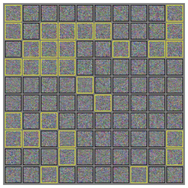
Figure 5: Randomly generated fooling images for a convolutional network trained on CIFAR-10. These examples were generated by drawing a sample from an isotropic Gaussian, then taking a gradient sign step in the direction that increases the probability of the “airplane” class. Yellow boxes indicate samples that successfully fool the model into believing an airplane is present with at least 50% confidence. “Airplane” is the hardest class to construct fooling images for on CIFAR-10, so this figure represents the worst case in terms of success rate.

图 5：为在 CIFAR-10 上训练的卷积网络随机生成的愚弄图像。这些例子的生成方式是：先从各向同性高斯中抽取一个样本，再沿着提高“飞机”类概率的方向走一步梯度符号。黄框标出成功把模型骗成相信有飞机存在、且把握至少为 50% 的样本。“飞机”是 CIFAR-10 上构造愚弄图像最难的类，因此本图代表的是成功率意义上的最坏情况。

We found that we were able to train a maxout network to have a zero percent error rate on Gaussian rubbish examples (it was still vulnerable to rubbish examples generated by applying a fast gradient sign step to a Gaussian sample) with no negative impact on its ability to classify clean examples. Unfortunately, unlike training on adversarial examples, this did not result in any significant reduction of the model’s test set error rate.

我们发现，能够把一个 maxout 网络训练到在高斯垃圾例子上误差率为零（它仍然容易受到对高斯样本再走一步快速梯度符号所生成的垃圾例子的攻击），而且不会对其分类干净例子的能力产生负面影响。遗憾的是，与在对抗样本上训练不同，这并没有显著降低模型的测试集误差率。

In conclusion, it appears that a randomly selected input to deep or shallow models built from linear parts is overwhelmingly likely to be processed incorrectly, and that these models only behave reasonably on a very thin manifold encompassing the training data.

总而言之，一个随机选取的输入，送进由线性部件构成的深层或浅层模型时，被错误处理的可能性占压倒多数；这些模型只在包围训练数据的那条非常薄的流形上，才会表现得合理。