End-To-End Memory Networks
End-To-End Memory Networks
Abstract
摘要
We introduce a neural network with a recurrent attention model over a possibly large external memory. The architecture is a form of Memory Network [23] but unlike the model in that work, it is trained end-to-end, and hence requires significantly less supervision during training, making it more generally applicable in realistic settings. It can also be seen as an extension of RNNsearch [2] to the case where multiple computational steps (hops) are performed per output symbol. The flexibility of the model allows us to apply it to tasks as diverse as (synthetic) question answering [22] and to language modeling. For the former our approach is competitive with Memory Networks, but with less supervision. For the latter, on the Penn TreeBank and Text8 datasets our approach demonstrates comparable performance to RNNs and LSTMs. In both cases we show that the key concept of multiple computational hops yields improved results.
我们提出一种带有循环注意力模型、作用在可能很大的外部记忆上的神经网络。该结构是记忆网络(Memory Network)[23] 的一种形式,但与那项工作中的模型不同,它是端到端训练的,因而在训练时需要的监督明显更少,在现实设定中也更一般地适用。它也可以看成把 RNNsearch [2] 扩展到每个输出符号执行多个计算步骤(跳,hops)的情形。模型的灵活性使我们能把它用到彼此很不相同的任务上,例如(合成)问答 [22] 和语言建模。对前者,我们的方法与记忆网络有竞争力,但所需监督更少。对后者,在 Penn TreeBank 和 Text8 数据集上,我们的方法表现出与 RNN 和 LSTM 相当的性能。在这两种情形下,我们都表明,多个计算跳这一关键概念会带来更好的结果。
1 Introduction
1 引言
Two grand challenges in artificial intelligence research have been to build models that can make multiple computational steps in the service of answering a question or completing a task, and models that can describe long term dependencies in sequential data.
人工智能研究里有两项重大挑战:一是建立能够为回答问题或完成任务而执行多个计算步骤的模型,二是建立能够刻画序列数据中长期依赖的模型。
Recently there has been a resurgence in models of computation using explicit storage and a notion of attention [23, 8, 2]; manipulating such a storage offers an approach to both of these challenges. In [23, 8, 2], the storage is endowed with a continuous representation; reads from and writes to the storage, as well as other processing steps, are modeled by the actions of neural networks.
近来,使用显式存储并带有注意力概念的计算模型重新受到关注 [23, 8, 2];操作这样的存储,为上述两项挑战都提供了一条途径。在 [23, 8, 2] 中,存储被赋予连续表示;对存储的读和写,以及其他处理步骤,都由神经网络的动作来建模。
In this work, we present a novel recurrent neural network (RNN) architecture where the recurrence reads from a possibly large external memory multiple times before outputting a symbol. Our model can be considered a continuous form of the Memory Network implemented in [23]. The model in that work was not easy to train via backpropagation, and required supervision at each layer of the network. The continuity of the model we present here means that it can be trained end-to-end from input-output pairs, and so is applicable to more tasks, i.e. tasks where such supervision is not available, such as in language modeling or realistically supervised question answering tasks. Our model can also be seen as a version of RNNsearch [2] with multiple computational steps (which we term "hops") per output symbol. We will show experimentally that the multiple hops over the long-term memory are crucial to good performance of our model on these tasks, and that training the memory representation can be integrated in a scalable manner into our end-to-end neural network model.
在本工作中,我们提出一种新的循环神经网络(RNN)结构:在输出一个符号之前,循环会多次读取可能很大的外部记忆。我们的模型可以看成 [23] 中所实现记忆网络的连续形式。那项工作中的模型不容易用反向传播训练,并且需要在网络的每一层提供监督。我们这里提出的模型是连续的,这意味着它可以从输入输出对端到端训练,因而可以用于更多任务,也就是那些没有此类监督的任务,例如语言建模,或监督更为现实的问答任务。我们的模型也可以看成每输出一个符号就做多个计算步骤(我们称之为“跳”)的 RNNsearch [2] 变体。我们将用实验表明,对长期记忆做多次跳,对我们的模型在这些任务上取得良好性能至关重要,并且对记忆表示的训练可以可扩展地整合进我们的端到端神经网络模型。
2 Approach
2 方法
Our model takes a discrete set of inputs that are to be stored in the memory, a query , and outputs an answer . Each of the , , and contains symbols coming from a dictionary with words. The model writes all to the memory up to a fixed buffer size, and then finds a continuous representation for the and . The continuous representation is then processed via multiple hops to output . This allows backpropagation of the error signal through multiple memory accesses back to the input during training.
我们的模型接收一组要存入记忆的离散输入 、一个查询 ,并输出一个答案 。每个 、 和 都包含来自一个有 个词的词典中的符号。模型把所有 写入记忆,直到固定的缓冲大小,然后为 和 找到连续表示。再经多次跳处理这一连续表示,输出 。这使得训练时可以把误差信号经多次记忆访问反向传播回输入。
2.1 Single Layer
2.1 单层
We start by describing our model in the single layer case, which implements a single memory hop operation. We then show it can be stacked to give multiple hops in memory.
我们先描述单层情形下的模型,它实现一次记忆跳操作。然后说明如何把它堆叠起来,以在记忆上做多次跳。
Input memory representation: Suppose we are given an input set to be stored in memory. The entire set of are converted into memory vectors of dimension computed by embedding each in a continuous space, in the simplest case, using an embedding matrix (of size ). The query is also embedded (again, in the simplest case via another embedding matrix with the same dimensions as ) to obtain an internal state . In the embedding space, we compute the match between and each memory by taking the inner product followed by a softmax:
输入记忆表示:假设给定一组要存入记忆的输入 。整个集合 被转换成维度为 的记忆向量 ,其计算方式是把每个 嵌入到一个连续空间;在最简单的情形下,使用一个大小为 的嵌入矩阵 。查询 也被嵌入(同样,在最简单的情形下,经由另一个与 维数相同的嵌入矩阵 ),得到内部状态 。在嵌入空间中,我们通过对 与每个记忆 做内积再接 softmax,来计算二者的匹配:
where . Defined in this way is a probability vector over the inputs.
其中 。如此定义后, 是输入上的一个概率向量。
Output memory representation: Each has a corresponding output vector (given in the simplest case by another embedding matrix ). The response vector from the memory is then a sum over the transformed inputs , weighted by the probability vector from the input:
输出记忆表示:每个 有一个对应的输出向量 (在最简单的情形下由另一个嵌入矩阵 给出)。记忆给出的响应向量 则是对变换后的输入 按输入侧得到的概率向量加权求和:
Because the function from input to output is smooth, we can easily compute gradients and backpropagate through it. Other recently proposed forms of memory or attention take this approach, notably Bahdanau et al. [2] and Graves et al. [8], see also [9].
由于从输入到输出的函数是光滑的,我们可以容易地计算梯度并沿它反向传播。其他近来提出的记忆或注意力形式也采用这一做法,尤其是 Bahdanau 等人 [2] 和 Graves 等人 [8],另见 [9]。
Generating the final prediction: In the single layer case, the sum of the output vector and the input embedding is then passed through a final weight matrix (of size ) and a softmax to produce the predicted label:
生成最终预测:在单层情形下,把输出向量 与输入嵌入 之和送入一个最终的权重矩阵 (大小为 )和 softmax,以产生预测标签:
The overall model is shown in Fig. 1(a). During training, all three embedding matrices , and , as well as are jointly learned by minimizing a standard cross-entropy loss between and the true label . Training is performed using stochastic gradient descent (see Section 4.2 for more details).
整体模型见图 1(a)。训练时,三个嵌入矩阵 、 和 以及 一起学习,目标是最小化 与真实标签 之间的标准交叉熵损失。训练使用随机梯度下降(更多细节见第 4.2 节)。
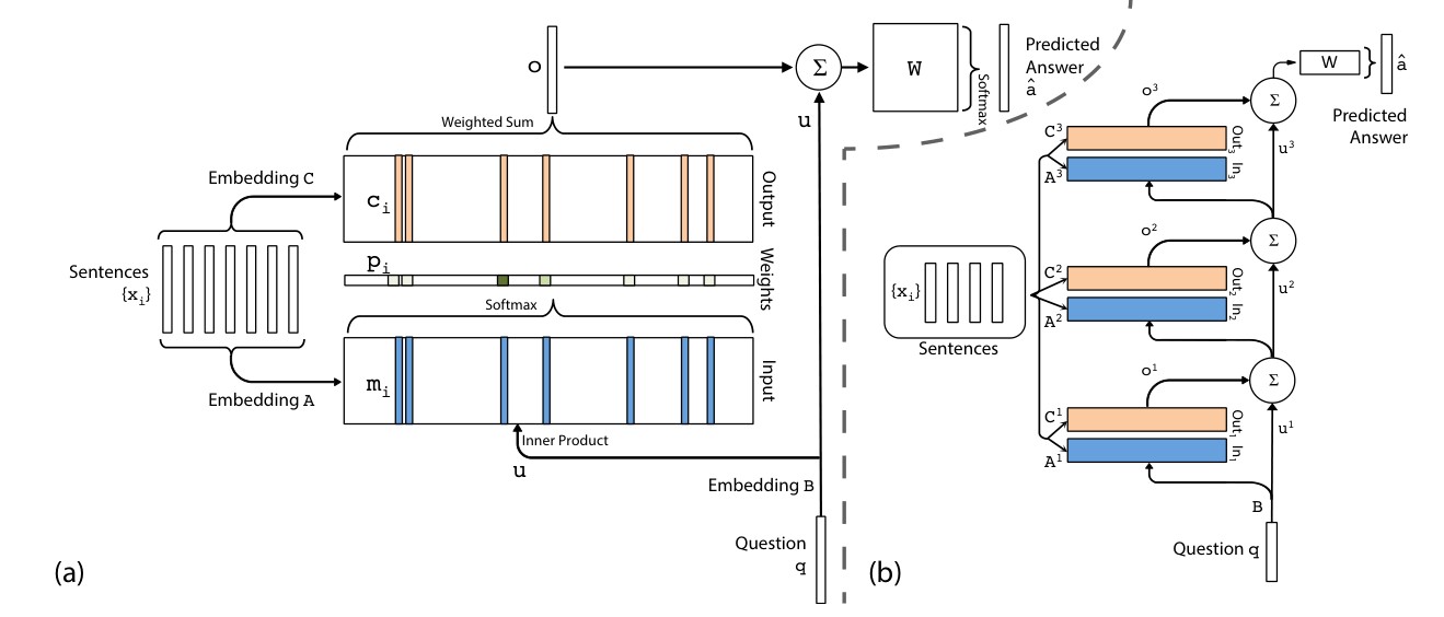
Figure 1: (a): A single layer version of our model. (b): A three layer version of our model. In practice, we can constrain several of the embedding matrices to be the same (see Section 2.2).
图 1:(a):我们模型的单层版本。(b):我们模型的三层版本。实践中,我们可以约束若干嵌入矩阵相同(见第 2.2 节)。
2.2 Multiple Layers
2.2 多层
We now extend our model to handle hop operations. The memory layers are stacked in the following way:
我们现在把模型扩展到处理 次跳操作。记忆层按如下方式堆叠:
- The input to layers above the first is the sum of the output and the input from layer (different ways to combine and are proposed later): . (4)
- 第一层以上各层的输入,是第 层的输出 与输入 之和(后面还提出了组合 与 的其他方式):。(4)
- Each layer has its own embedding matrices , , used to embed the inputs . However, as discussed below, they are constrained to ease training and reduce the number of parameters.
- 每一层有自己的嵌入矩阵 、,用来嵌入输入 。不过如下所述,它们会受到约束,以便于训练并减少参数量。
- At the top of the network, the input to also combines the input and the output of the top memory layer: .
- 在网络顶部,送入 的输入同样结合了顶层记忆层的输入与输出:。
We explore two types of weight tying within the model:
我们在模型内部探索了两类权值绑定:
- Adjacent: the output embedding for one layer is the input embedding for the one above, i.e. . We also constrain (a) the answer prediction matrix to be the same as the final output embedding, i.e , and (b) the question embedding to match the input embedding of the first layer, i.e. .
- 相邻绑定:一层的输出嵌入是上一层的输入嵌入,即 。我们还约束 (a) 答案预测矩阵与最后的输出嵌入相同,即 ,以及 (b) 问题嵌入与第一层的输入嵌入一致,即 。
- Layer-wise (RNN-like): the input and output embeddings are the same across different layers, i.e. and . We have found it useful to add a linear mapping to the update of between hops; that is, . This mapping is learnt along with the rest of the parameters and used throughout our experiments for layer-wise weight tying.
- 层间绑定(类似 RNN):不同层的输入、输出嵌入相同,即 以及 。我们发现,在各跳之间对 的更新加上一个线性映射 是有用的,也就是 。这一映射与其余参数一起学习,并在我们所有使用层间权值绑定的实验中采用。
A three-layer version of our memory model is shown in Fig. 1(b). Overall, it is similar to the Memory Network model in [23], except that the hard max operations within each layer have been replaced with a continuous weighting from the softmax.
我们记忆模型的三层版本见图 1(b)。总体而言,它与 [23] 中的记忆网络模型相似,只是每一层内的硬 max 操作被换成了来自 softmax 的连续加权。
Note that if we use the layer-wise weight tying scheme, our model can be cast as a traditional RNN where we divide the outputs of the RNN into internal and external outputs. Emitting an internal output corresponds to considering a memory, and emitting an external output corresponds to predicting a label. From the RNN point of view, in Fig. 1(b) and Eqn. 4 is a hidden state, and the model generates an internal output (attention weights in Fig. 1(a)) using . The model then ingests using , updates the hidden state, and so on. Here, unlike a standard RNN, we explicitly condition on the outputs stored in memory during the hops, and we keep these outputs soft, rather than sampling them. Thus our model makes several computational steps before producing an output meant to be seen by the "outside world".
注意,如果使用层间权值绑定方案,我们的模型可以写成一种传统 RNN,只是我们把 RNN 的输出分成内部输出和外部输出。发出内部输出对应于考虑一条记忆,发出外部输出对应于预测一个标签。从 RNN 的角度看,图 1(b) 和式 (4) 中的 是隐状态,模型用 生成内部输出 (也就是图 1(a) 中的注意力权重)。模型再用 吞入 ,更新隐状态,如此继续。与标准 RNN 不同的是,我们在 次跳期间显式地以存储在记忆中的输出为条件,并且保持这些输出是软的,而不是对它们做采样。因此,我们的模型在产生一个打算给“外部世界”看到的输出之前,会先做若干计算步骤。
Note that in this view, the terminology of input and output from Fig. 1 is flipped - when viewed as a traditional RNN with this special conditioning of outputs, becomes part of the output embedding of the RNN and becomes the input embedding.
注意,在这一视角下,图 1 中输入与输出的用语是对调的:当把它看成带有这种特殊输出条件的传统 RNN 时, 成为 RNN 输出嵌入的一部分,而 成为输入嵌入。
3 Related Work
3 相关工作
A number of recent efforts have explored ways to capture long-term structure within sequences using RNNs or LSTM-based models [4, 7, 12, 15, 10, 1]. The memory in these models is the state of the network, which is latent and inherently unstable over long timescales. The LSTM-based models address this through local memory cells which lock in the network state from the past. In practice, the performance gains over carefully trained RNNs are modest (see Mikolov et al. [15]). Our model differs from these in that it uses a global memory, with shared read and write functions. However, with layer-wise weight tying our model can be viewed as a form of RNN which only produces an output after a fixed number of time steps (corresponding to the number of hops), with the intermediary steps involving memory input/output operations that update the internal state.
近来已有不少工作探索用 RNN 或基于 LSTM 的模型来捕捉序列中的长期结构 [4, 7, 12, 15, 10, 1]。这些模型中的记忆就是网络的状态,它是隐变量,并且在长时尺度上天生不稳定。基于 LSTM 的模型通过局部记忆单元来应对这一点,这些单元会锁定过去的网络状态。实践中,相对仔细训练的 RNN,性能提升是有限的(见 Mikolov 等人 [15])。我们的模型与它们的不同在于使用全局记忆,并共享读写函数。不过,在使用层间权值绑定时,我们的模型可以看成一种只在固定数目的时间步(对应跳数)之后才产生输出的 RNN,中间步骤则包含用于更新内部状态的记忆输入/输出操作。
Some of the very early work on neural networks by Steinbuch and Piske[19] and Taylor [21] considered a memory that performed nearest-neighbor operations on stored input vectors and then fit parametric models to the retrieved sets. This has similarities to a single layer version of our model.
Steinbuch 与 Piske[19] 以及 Taylor [21] 在神经网络的一些很早期工作中,考虑过一种先对存储的输入向量做最近邻操作、再对取回的集合拟合参数模型的记忆。这与我们模型的单层版本有相似之处。
Subsequent work in the 1990's explored other types of memory [18, 5, 16]. For example, Das et al. [5] and Mozer et al. [16] introduced an explicit stack with push and pop operations which has been revisited recently by [11] in the context of an RNN model.
20 世纪 90 年代的后续工作探索了其他类型的记忆 [18, 5, 16]。例如,Das 等人 [5] 和 Mozer 等人 [16] 引入了带有压入和弹出操作的显式栈,这一想法近来又被 [11] 放在 RNN 模型的语境中重新讨论。
Closely related to our model is the Neural Turing Machine of Graves et al. [8], which also uses a continuous memory representation. The NTM memory uses both content and address-based access, unlike ours which only explicitly allows the former, although the temporal features that we will introduce in Section 4.1 allow a kind of address-based access. However, in part because we always write each memory sequentially, our model is somewhat simpler, not requiring operations like sharpening. Furthermore, we apply our memory model to textual reasoning tasks, which qualitatively differ from the more abstract operations of sorting and recall tackled by the NTM.
与我们的模型密切相关的是 Graves 等人 [8] 的神经图灵机,它也使用连续的记忆表示。NTM 的记忆同时使用基于内容和基于地址的访问,而我们的模型只显式允许前者,尽管我们将在第 4.1 节引入的时间特征允许一种基于地址的访问。不过,部分因为我们总是按顺序写入每条记忆,我们的模型更为简单,不需要锐化一类操作。此外,我们把记忆模型用到文本推理任务上,这与 NTM 所处理的排序和回忆等更抽象的操作在性质上不同。
Our model is also related to Bahdanau et al. [2]. In that work, a bidirectional RNN based encoder and gated RNN based decoder were used for machine translation. The decoder uses an attention model that finds which hidden states from the encoding are most useful for outputting the next translated word; the attention model uses a small neural network that takes as input a concatenation of the current hidden state of the decoder and each of the encoders hidden states. A similar attention model is also used in Xu et al. [24] for generating image captions. Our "memory" is analogous to their attention mechanism, although [2] is only over a single sentence rather than many, as in our case. Furthermore, our model makes several hops on the memory before making an output; we will see below that this is important for good performance. There are also differences in the architecture of the small network used to score the memories compared to our scoring approach; we use a simple linear layer, whereas they use a more sophisticated gated architecture.
我们的模型也与 Bahdanau 等人 [2] 有关。那项工作把基于双向 RNN 的编码器和基于门控 RNN 的解码器用于机器翻译。解码器使用一个注意力模型,找出编码中哪些隐状态对输出下一个译词最有用;该注意力模型使用一个小神经网络,其输入是解码器当前隐状态与编码器各个隐状态的拼接。类似的注意力模型也被 Xu 等人 [24] 用于生成图像描述。我们的“记忆”类似于他们的注意力机制,不过 [2] 只作用在一个句子上,而我们的情形是许多句子。此外,我们的模型在给出输出之前会对记忆做多次跳;下面将会看到,这对取得良好性能很重要。用来给记忆打分的小网络结构也与我们的打分方法不同:我们使用简单的线性层,而他们使用更复杂的门控结构。
We will apply our model to language modeling, an extensively studied task. Goodman [6] showed simple but effective approaches which combine n-grams with a cache. Bengio et al. [3] ignited interest in using neural network based models for the task, with RNNs [14] and LSTMs [10, 20] showing clear performance gains over traditional methods. Indeed, the current state-of-the-art is held by variants of these models, for example very large LSTMs with Dropout [25] or RNNs with diagonal constraints on the weight matrix [15]. With appropriate weight tying, our model can be regarded as a modified form of RNN, where the recurrence is indexed by memory lookups to the word sequence rather than indexed by the sequence itself.
我们将把模型用到语言建模这一被广泛研究的任务上。Goodman [6] 给出了把 n-gram 与缓存结合起来的简单而有效的方法。Bengio 等人 [3] 激发了用基于神经网络的模型做这一任务的兴趣,RNN [14] 和 LSTM [10, 20] 相对传统方法表现出明显的性能提升。事实上,当时最好的结果由这些模型的变体保持,例如带 Dropout 的很大的 LSTM [25],或对权重矩阵施加对角约束的 RNN [15]。在适当的权值绑定下,我们的模型可以看成一种改过的 RNN,其循环是按对词序列的记忆查找来索引的,而不是按序列本身来索引。
4 Synthetic Question and Answering Experiments
4 合成问答实验
We perform experiments on the synthetic QA tasks defined in [22] (using version 1.1 of the dataset). A given QA task consists of a set of statements, followed by a question whose answer is typically a single word (in a few tasks, answers are a set of words). The answer is available to the model at training time, but must be predicted at test time. There are a total of 20 different types of tasks that probe different forms of reasoning and deduction. Here are samples of three of the tasks:
我们在 [22] 定义的合成问答任务上做实验(使用该数据集的 1.1 版)。一个给定的问答任务由一组陈述和一个问题组成,答案通常是单个词(在少数任务中,答案是一组词)。训练时模型可以看到答案,测试时则必须预测答案。一共有 20 种不同类型的任务,分别探查不同形式的推理和演绎。下面是其中三个任务的样例:
Sam walks into the kitchen.
Sam picks up an apple.
Sam walks into the bedroom.
Sam drops the apple.
Q: Where is the apple?
A. Bedroom
Brian is a lion.
Julius is a lion.
Julius is white.
Bernhard is green.
Q: What color is Brian?
A. White
Mary journeyed to the den.
Mary went back to the kitchen.
John journeyed to the bedroom.
Mary discarded the milk.
Q: Where was the milk before the den?
A. Hallway
Note that for each question, only some subset of the statements contain information needed for the answer, and the others are essentially irrelevant distractors (e.g. the first sentence in the first example). In the Memory Networks of Weston et al. [22], this supporting subset was explicitly indicated to the model during training and the key difference between that work and this one is that this information is no longer provided. Hence, the model must deduce for itself at training and test time which sentences are relevant and which are not.
注意,对每个问题,只有一部分陈述包含答案所需的信息,其余本质上是无关的干扰(例如第一个例子中的第一句)。在 Weston 等人 [22] 的记忆网络中,这一支撑子集在训练时被明确告知模型;那项工作与本文的关键区别是,这一信息不再提供。因此,模型必须在训练和测试时自己推断哪些句子相关、哪些不相关。
Formally, for one of the 20 QA tasks, we are given example problems, each having a set of sentences where ; a question sentence and answer . Let the th word of sentence be , represented by a one-hot vector of length (where the vocabulary is of size , reflecting the simplistic nature of the QA language). The same representation is used for the question and answer . Two versions of the data are used, one that has 1000 training problems per task and a second larger one with 10,000 per task.
形式化地说,对 20 个问答任务中的一个,我们得到若干例题,每题有一组 个句子 ,其中 ;一个问句 和答案 。设句子 的第 个词为 ,用长度为 的独热向量表示(词表大小 ,反映出问答语言的简单性质)。问题 和答案 使用同样的表示。数据使用两个版本,一个是每项任务 1000 道训练题,另一个更大的版本每项任务 10,000 道。
4.1 Model Details
4.1 模型细节
Unless otherwise stated, all experiments used a hops model with the adjacent weight sharing scheme. For all tasks that output lists (i.e. the answers are multiple words), we take each possible combination of possible outputs and record them as a separate answer vocabulary word.
除非另有说明,全部实验都使用 跳、并采用相邻权值共享方案的模型。对所有输出列表的任务(即答案是多个词),我们把可能输出的每一种组合记为答案词表中的一个单独词。
Sentence Representation: In our experiments we explore two different representations for the sentences. The first is the bag-of-words (BoW) representation that takes the sentence , embeds each word and sums the resulting vectors: e.g and . The input vector representing the question is also embedded as a bag of words: . This has the drawback that it cannot capture the order of the words in the sentence, which is important for some tasks.
句子表示:在实验中我们探索两种不同的句子表示。第一种是词袋(BoW)表示:取句子 ,把每个词嵌入后再把得到的向量相加,例如 以及 。表示问题的输入向量 也按词袋嵌入:。其缺点是无法捕捉句子中的词序,而这对某些任务很重要。
We therefore propose a second representation that encodes the position of words within the sentence. This takes the form: , where is an element-wise multiplication. is a column vector with the structure (assuming 1-based indexing), with being the number of words in the sentence, and is the dimension of the embedding. This sentence representation, which we call position encoding (PE), means that the order of the words now affects . The same representation is used for questions, memory inputs and memory outputs.
因此我们提出第二种表示,对句子中词的位置进行编码。其形式为:,其中 是逐元素相乘。 是一个列向量,结构为 (假定下标从 1 开始),其中 是句子中的词数, 是嵌入维数。我们把这种句子表示称为位置编码(PE),它意味着词的顺序现在会影响 。问题、记忆输入和记忆输出使用同一种表示。
Temporal Encoding: Many of the QA tasks require some notion of temporal context, i.e. in the first example of Section 2, the model needs to understand that Sam is in the bedroom after he is in the kitchen. To enable our model to address them, we modify the memory vector so that , where is the th row of a special matrix that encodes temporal information. The output embedding is augmented in the same way with a matrix (e.g. ). Both and are learned during training. They are also subject to the same sharing constraints as and . Note that sentences are indexed in reverse order, reflecting their relative distance from the question so that is the last sentence of the story.
时间编码:许多问答任务需要某种时间上下文的概念,例如在第 2 节的第一个例子中,模型需要理解 Sam 是在厨房之后才到卧室的。为使模型能够处理这些任务,我们修改记忆向量,使得 ,其中 是编码时间信息的特殊矩阵 的第 行。输出嵌入以同样方式用矩阵 加以扩充(例如 )。 和 都在训练中学习,并且也受与 和 相同的共享约束。注意,句子按逆序编号,以反映它们相对问题的距离,因此 是故事中的最后一句。
Learning time invariance by injecting random noise: we have found it helpful to add "dummy" memories to regularize . That is, at training time we can randomly add 10% of empty memories to the stories. We refer to this approach as random noise (RN).
通过注入随机噪声来学习时间不变性:我们发现,加入“哑”记忆来正则化 是有帮助的。也就是说,在训练时我们可以随机向故事中加入 10% 的空记忆。我们把这种方法称为随机噪声(RN)。
4.2 Training Details
4.2 训练细节
10% of the bAbI training set was held-out to form a validation set, which was used to select the optimal model architecture and hyperparameters. Our models were trained using a learning rate of , with anneals every 25 epochs by until 100 epochs were reached. No momentum or weight decay was used. The weights were initialized randomly from a Gaussian distribution with zero mean and . When trained on all tasks simultaneously with 1k training samples (10k training samples), 60 epochs (20 epochs) were used with learning rate anneals of every 15 epochs (5 epochs). All training uses a batch size of 32 (but cost is not averaged over a batch), and gradients with an norm larger than 40 are divided by a scalar to have norm 40. In some of our experiments, we explored commencing training with the softmax in each memory layer removed, making the model entirely linear except for the final softmax for answer prediction. When the validation loss stopped decreasing, the softmax layers were re-inserted and training recommenced. We refer to this as linear start (LS) training. In LS training, the initial learning rate is set to . The capacity of memory is restricted to the most recent 50 sentences. Since the number of sentences and the number of words per sentence varied between problems, a null symbol was used to pad them all to a fixed size. The embedding of the null symbol was constrained to be zero.
bAbI 训练集中有 10% 被留出作为验证集,用来选择最优的模型结构和超参数。我们的模型用学习率 训练,每 25 个 epoch 把学习率退火为 ,直到 100 个 epoch。不使用动量或权重衰减。权重从均值为零、 的高斯分布随机初始化。当用 1k 训练样本(10k 训练样本)在全部任务上同时训练时,使用 60 个 epoch(20 个 epoch),并每 15 个 epoch(5 个 epoch)把学习率退火为 。全部训练的批量大小为 32(但代价不在一个批量上取平均), 范数大于 40 的梯度会被一个标量除掉,使其范数为 40。在部分实验中,我们探索先去掉每一记忆层中的 softmax 再开始训练,使模型除最后用于答案预测的 softmax 外完全是线性的。当验证损失停止下降时,再把 softmax 层插回去继续训练。我们称之为线性启动(LS)训练。在 LS 训练中,初始学习率设为 。记忆容量限制为最近的 50 个句子。由于不同题目的句子数以及每句词数不同,用一个空符号把它们都填充到固定大小。空符号的嵌入被约束为零。
On some tasks, we observed a large variance in the performance of our model (i.e. sometimes failing badly, other times not, depending on the initialization). To remedy this, we repeated each training 10 times with different random initializations, and picked the one with the lowest training error.
在某些任务上,我们观察到模型性能有很大方差(也就是说,有时失败得很严重,有时则不然,取决于初始化)。为补救这一点,我们用不同的随机初始化把每次训练重复 10 遍,并选取训练误差最低的那一次。
4.3 Baselines
4.3 基线
We compare our approach (abbreviated to MemN2N) to a range of alternate models:
我们把我们的方法(简写为 MemN2N)与一系列替代模型做比较:
MemN2N source code is available at https://github.com/facebook/MemNN.
MemN2N 的源代码见 https://github.com/facebook/MemNN。
- MemNN: The strongly supervised AM+NG+NL Memory Networks approach, proposed in [22]. This is the best reported approach in that paper. It uses a max operation (rather than softmax) at each layer which is trained directly with supporting facts (strong supervision). It employs n-gram modeling, nonlinear layers and an adaptive number of hops per query.
- MemNN: [22] 中提出的强监督 AM+NG+NL 记忆网络方法。这是该文报告的最好方法。它在每一层使用 max 操作(而不是 softmax),并直接用支撑事实训练(强监督)。它采用 n-gram 建模、非线性层,以及每个查询自适应的跳数。
- MemNN-WSH: A weakly supervised heuristic version of MemNN where the supporting sentence labels are not used in training. Since we are unable to backpropagate through the max operations in each layer, we enforce that the first memory hop should share at least one word with the question, and that the second memory hop should share at least one word with the first hop and at least one word with the answer. All those memories that conform are called valid memories, and the goal during training is to rank them higher than invalid memories using the same ranking criteria as during strongly supervised training.
- MemNN-WSH:MemNN 的弱监督启发式版本,训练时不使用支撑句标签。由于无法通过各层中的 max 操作反向传播,我们要求第一次记忆跳至少与问题共享一个词,第二次记忆跳至少与第一次跳共享一个词、并且至少与答案共享一个词。所有符合这些条件的记忆称为有效记忆,训练时的目标是用与强监督训练相同的排序准则,把它们排在无效记忆之上。
- LSTM: A standard LSTM model, trained using question / answer pairs only (i.e. also weakly supervised). For more detail, see [22].
- LSTM:一个标准的 LSTM 模型,只用问题/答案对训练(也就是说,同样是弱监督的)。更多细节见 [22]。
4.4 Results
4.4 结果
We report a variety of design choices: (i) BoW vs Position Encoding (PE) sentence representation; (ii) training on all 20 tasks independently vs jointly training (joint training used an embedding dimension of , while independent training used ); (iii) two phase training: linear start (LS) where softmaxes are removed initially vs training with softmaxes from the start; (iv) varying memory hops from 1 to 3.
我们报告多种设计选择:(i) 词袋(BoW)与位置编码(PE)句子表示;(ii) 在全部 20 项任务上独立训练还是联合训练(联合训练使用嵌入维数 ,独立训练使用 );(iii) 两阶段训练:先去掉 softmax 的线性启动(LS),还是从一开始就带 softmax 训练;(iv) 把记忆跳数从 1 变到 3。
The results across all 20 tasks are given in Table 1 for the 1k training set, along with the mean performance for 10k training set. They show a number of interesting points:
全部 20 项任务在 1k 训练集上的结果见表 1,同时还给出了 10k 训练集上的平均成绩。它们显示出若干有意思的要点:
More detailed results for the 10k training set can be found in the supplementary material.
10k 训练集上更详细的结果见补充材料。
- The best MemN2N models are reasonably close to the supervised models (e.g. 1k: 6.7% for MemNN vs 12.6% for MemN2N with position encoding + linear start + random noise, jointly trained and 10k: 3.2% for MemNN vs 4.2% for MemN2N with position encoding + linear start + random noise + non-linearity, although the supervised models are still superior.
- 最好的 MemN2N 模型与有监督模型相当接近(例如,1k:MemNN 为 6.7%,带位置编码 + 线性启动 + 随机噪声并联合训练的 MemN2N 为 12.6%;10k:MemNN 为 3.2%,带位置编码 + 线性启动 + 随机噪声 + 非线性的 MemN2N 为 4.2%),尽管有监督模型仍然更好。
Following [17] we found adding more non-linearity solves tasks 17 and 19, see the supplementary material.
沿用 [17],我们发现增加更多非线性可以解决第 17 和 19 项任务,见补充材料。
- All variants of our proposed model comfortably beat the weakly supervised baseline methods.
- 我们提出的模型的所有变体都明显超过弱监督基线方法。
- The position encoding (PE) representation improves over bag-of-words (BoW), as demonstrated by clear improvements on tasks 4, 5, 15 and 18, where word ordering is particularly important.
- 位置编码(PE)表示优于词袋(BoW),这在第 4、5、15 和 18 项对词序特别重要的任务上有明显改进。
- The linear start (LS) to training seems to help avoid local minima. See task 16 in Table 1, where PE alone gets 53.6% error, while using LS reduces it to 1.6%.
- 训练的线性启动(LS)似乎有助于避开局部极小。见表 1 中的第 16 项:单独用 PE 的错误率是 53.6%,而使用 LS 后降到 1.6%。
- Jittering the time index with random empty memories (RN) as described in Section 4.1 gives a small but consistent boost in performance, especially for the smaller 1k training set.
- 如第 4.1 节所述,用随机空记忆扰动时间索引(RN),会带来虽然不大、但稳定的性能提升,尤其是在较小的 1k 训练集上。
- Joint training on all tasks helps.
- 在全部任务上联合训练是有帮助的。
- Importantly, more computational hops give improved performance. We give examples of the hops performed (via the values of eq. (1)) over some illustrative examples in Fig. 2 and in the supplementary material.
- 重要的是,更多的计算跳会带来更好的性能。我们在图 2 和补充材料中,通过式 (1) 的取值,给出了一些说明性例子上所执行的跳。
| Task | MemNN [22] | LSTM [22] | MemNN WSH | BoW | PE | PE LS | PE LS RN | PE joint | PE LS joint | 1 hop PE LS joint | 2 hops PE LS joint | 3 hops PE LS RN joint | PE LS LW joint |
|---|---|---|---|---|---|---|---|---|---|---|---|---|---|
| 1: 1 supporting fact | 0.0 | 50.0 | 0.1 | 0.6 | 0.1 | 0.2 | 0.0 | 0.8 | 0.0 | 0.1 | 0.0 | 0.1 | |
| 2: 2 supporting facts | 0.0 | 80.0 | 42.8 | 17.6 | 21.6 | 12.8 | 8.3 | 62.0 | 15.6 | 14.0 | 11.4 | 18.8 | |
| 3: 3 supporting facts | 0.0 | 80.0 | 76.4 | 71.0 | 64.2 | 58.8 | 40.3 | 76.9 | 31.6 | 33.1 | 21.9 | 31.7 | |
| 4: 2 argument relations | 0.0 | 39.0 | 40.3 | 32.0 | 3.8 | 11.6 | 2.8 | 22.8 | 2.2 | 5.7 | 13.4 | 17.5 | |
| 5: 3 argument relations | 2.0 | 30.0 | 16.3 | 18.3 | 14.1 | 15.7 | 13.1 | 11.0 | 13.4 | 14.8 | 14.4 | 12.9 | |
| 6: yes/no questions | 0.0 | 52.0 | 51.0 | 8.7 | 7.9 | 8.7 | 7.6 | 7.2 | 2.3 | 3.3 | 2.8 | 2.0 | |
| 7: counting | 15.0 | 51.0 | 36.1 | 23.5 | 21.6 | 20.3 | 17.3 | 15.9 | 25.4 | 17.9 | 18.3 | 10.1 | |
| 8: lists/sets | 9.0 | 55.0 | 37.8 | 11.4 | 12.6 | 12.7 | 10.0 | 13.2 | 11.7 | 10.1 | 9.3 | 6.1 | |
| 9: simple negation | 0.0 | 36.0 | 35.9 | 21.1 | 23.3 | 17.0 | 13.2 | 5.1 | 2.0 | 3.1 | 1.9 | 1.5 | |
| 10: indefinite knowledge | 2.0 | 56.0 | 68.7 | 22.8 | 17.4 | 18.6 | 15.1 | 10.6 | 5.0 | 6.6 | 6.5 | 2.6 | |
| 11: basic coreference | 0.0 | 38.0 | 30.0 | 4.1 | 4.3 | 0.0 | 0.9 | 8.4 | 1.2 | 0.9 | 0.3 | 3.3 | |
| 12: conjunction | 0.0 | 26.0 | 10.1 | 0.3 | 0.3 | 0.1 | 0.2 | 0.4 | 0.0 | 0.3 | 0.1 | 0.0 | |
| 13: compound coreference | 0.0 | 6.0 | 19.7 | 10.5 | 9.9 | 0.3 | 0.4 | 6.3 | 0.2 | 1.4 | 0.2 | 0.5 | |
| 14: time reasoning | 1.0 | 73.0 | 18.3 | 1.3 | 1.8 | 2.0 | 1.7 | 36.9 | 8.1 | 8.2 | 6.9 | 2.0 | |
| 15: basic deduction | 0.0 | 79.0 | 64.8 | 24.3 | 0.0 | 0.0 | 0.0 | 46.4 | 0.5 | 0.0 | 0.0 | 1.8 | |
| 16: basic induction | 0.0 | 77.0 | 50.5 | 52.0 | 52.1 | 1.6 | 1.3 | 47.4 | 51.3 | 3.5 | 2.7 | 51.0 | |
| 17: positional reasoning | 35.0 | 49.0 | 50.9 | 45.4 | 50.1 | 49.0 | 51.0 | 44.4 | 41.2 | 44.5 | 40.4 | 42.6 | |
| 18: size reasoning | 5.0 | 48.0 | 51.3 | 48.1 | 13.6 | 10.1 | 11.1 | 9.6 | 10.3 | 9.2 | 9.4 | 9.2 | |
| 19: path finding | 64.0 | 92.0 | 100.0 | 89.7 | 87.4 | 85.6 | 82.8 | 90.7 | 89.9 | 90.2 | 88.0 | 90.6 | |
| 20: agent's motivation | 0.0 | 9.0 | 3.6 | 0.1 | 0.0 | 0.0 | 0.0 | 0.0 | 0.1 | 0.0 | 0.0 | 0.2 | |
| Mean error (%) | 6.7 | 51.3 | 40.2 | 25.1 | 20.3 | 16.3 | 13.9 | 25.8 | 15.6 | 13.3 | 12.4 | 15.2 | |
| Failed tasks (err. > 5%) | 4 | 20 | 18 | 15 | 13 | 12 | 11 | 17 | 11 | 11 | 11 | 10 | |
| On 10k training data Mean error (%) | 3.2 | 36.4 | 39.2 | 15.4 | 9.4 | 7.2 | 6.6 | 24.5 | 10.9 | 7.9 | 7.5 | 11.0 | |
| Failed tasks (err. > 5%) | 2 | 16 | 17 | 9 | 6 | 4 | 4 | 16 | 7 | 6 | 6 | 6 |
Table 1: Test error rates (%) on the 20 QA tasks for models using 1k training examples (mean test errors for 10k training examples are shown at the bottom). Key: BoW = bag-of-words representation; PE = position encoding representation; LS = linear start training; RN = random injection of time index noise; LW = RNN-style layer-wise weight tying (if not stated, adjacent weight tying is used); joint = joint training on all tasks (as opposed to per-task training).
| Task | MemNN [22] | LSTM [22] | MemNN WSH | BoW | PE | PE LS | PE LS RN | PE joint | PE LS joint | 1 hop PE LS joint | 2 hops PE LS joint | 3 hops PE LS RN joint | PE LS LW joint |
|---|---|---|---|---|---|---|---|---|---|---|---|---|---|
| 1: 1 supporting fact | 0.0 | 50.0 | 0.1 | 0.6 | 0.1 | 0.2 | 0.0 | 0.8 | 0.0 | 0.1 | 0.0 | 0.1 | |
| 2: 2 supporting facts | 0.0 | 80.0 | 42.8 | 17.6 | 21.6 | 12.8 | 8.3 | 62.0 | 15.6 | 14.0 | 11.4 | 18.8 | |
| 3: 3 supporting facts | 0.0 | 80.0 | 76.4 | 71.0 | 64.2 | 58.8 | 40.3 | 76.9 | 31.6 | 33.1 | 21.9 | 31.7 | |
| 4: 2 argument relations | 0.0 | 39.0 | 40.3 | 32.0 | 3.8 | 11.6 | 2.8 | 22.8 | 2.2 | 5.7 | 13.4 | 17.5 | |
| 5: 3 argument relations | 2.0 | 30.0 | 16.3 | 18.3 | 14.1 | 15.7 | 13.1 | 11.0 | 13.4 | 14.8 | 14.4 | 12.9 | |
| 6: yes/no questions | 0.0 | 52.0 | 51.0 | 8.7 | 7.9 | 8.7 | 7.6 | 7.2 | 2.3 | 3.3 | 2.8 | 2.0 | |
| 7: counting | 15.0 | 51.0 | 36.1 | 23.5 | 21.6 | 20.3 | 17.3 | 15.9 | 25.4 | 17.9 | 18.3 | 10.1 | |
| 8: lists/sets | 9.0 | 55.0 | 37.8 | 11.4 | 12.6 | 12.7 | 10.0 | 13.2 | 11.7 | 10.1 | 9.3 | 6.1 | |
| 9: simple negation | 0.0 | 36.0 | 35.9 | 21.1 | 23.3 | 17.0 | 13.2 | 5.1 | 2.0 | 3.1 | 1.9 | 1.5 | |
| 10: indefinite knowledge | 2.0 | 56.0 | 68.7 | 22.8 | 17.4 | 18.6 | 15.1 | 10.6 | 5.0 | 6.6 | 6.5 | 2.6 | |
| 11: basic coreference | 0.0 | 38.0 | 30.0 | 4.1 | 4.3 | 0.0 | 0.9 | 8.4 | 1.2 | 0.9 | 0.3 | 3.3 | |
| 12: conjunction | 0.0 | 26.0 | 10.1 | 0.3 | 0.3 | 0.1 | 0.2 | 0.4 | 0.0 | 0.3 | 0.1 | 0.0 | |
| 13: compound coreference | 0.0 | 6.0 | 19.7 | 10.5 | 9.9 | 0.3 | 0.4 | 6.3 | 0.2 | 1.4 | 0.2 | 0.5 | |
| 14: time reasoning | 1.0 | 73.0 | 18.3 | 1.3 | 1.8 | 2.0 | 1.7 | 36.9 | 8.1 | 8.2 | 6.9 | 2.0 | |
| 15: basic deduction | 0.0 | 79.0 | 64.8 | 24.3 | 0.0 | 0.0 | 0.0 | 46.4 | 0.5 | 0.0 | 0.0 | 1.8 | |
| 16: basic induction | 0.0 | 77.0 | 50.5 | 52.0 | 52.1 | 1.6 | 1.3 | 47.4 | 51.3 | 3.5 | 2.7 | 51.0 | |
| 17: positional reasoning | 35.0 | 49.0 | 50.9 | 45.4 | 50.1 | 49.0 | 51.0 | 44.4 | 41.2 | 44.5 | 40.4 | 42.6 | |
| 18: size reasoning | 5.0 | 48.0 | 51.3 | 48.1 | 13.6 | 10.1 | 11.1 | 9.6 | 10.3 | 9.2 | 9.4 | 9.2 | |
| 19: path finding | 64.0 | 92.0 | 100.0 | 89.7 | 87.4 | 85.6 | 82.8 | 90.7 | 89.9 | 90.2 | 88.0 | 90.6 | |
| 20: agent's motivation | 0.0 | 9.0 | 3.6 | 0.1 | 0.0 | 0.0 | 0.0 | 0.0 | 0.1 | 0.0 | 0.0 | 0.2 | |
| Mean error (%) | 6.7 | 51.3 | 40.2 | 25.1 | 20.3 | 16.3 | 13.9 | 25.8 | 15.6 | 13.3 | 12.4 | 15.2 | |
| Failed tasks (err. > 5%) | 4 | 20 | 18 | 15 | 13 | 12 | 11 | 17 | 11 | 11 | 11 | 10 | |
| On 10k training data Mean error (%) | 3.2 | 36.4 | 39.2 | 15.4 | 9.4 | 7.2 | 6.6 | 24.5 | 10.9 | 7.9 | 7.5 | 11.0 | |
| Failed tasks (err. > 5%) | 2 | 16 | 17 | 9 | 6 | 4 | 4 | 16 | 7 | 6 | 6 | 6 |
表 1:使用 1k 训练样本的模型在 20 项问答任务上的测试错误率(%)(10k 训练样本的平均测试错误列在表底)。代号:BoW = 词袋表示;PE = 位置编码表示;LS = 线性启动训练;RN = 对时间索引随机注入噪声;LW = RNN 式层间权值绑定(若未说明,则使用相邻权值绑定);joint = 在全部任务上联合训练(相对于逐任务训练)。
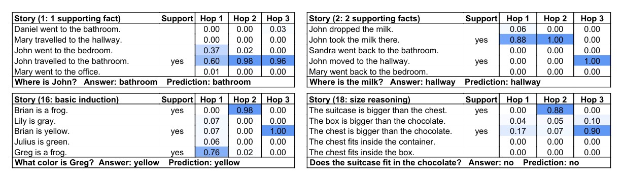
Figure 2: Example predictions on the QA tasks of [22]. We show the labeled supporting facts (support) from the dataset which MemN2N does not use during training, and the probabilities of each hop used by the model during inference. MemN2N successfully learns to focus on the correct supporting sentences.
图 2:[22] 的问答任务上的预测例子。我们给出数据集中已标注的支撑事实(support),MemN2N 在训练时并不使用它们,以及模型在推断时各次跳使用的概率 。MemN2N 成功地学会把注意力放到正确的支撑句上。
5 Language Modeling Experiments
5 语言建模实验
The goal in language modeling is to predict the next word in a text sequence given the previous words . We now explain how our model can easily be applied to this task.
语言建模的目标是在给定前面的词 时,预测文本序列中的下一个词。下面说明如何把我们的模型容易地用到这一任务上。
We now operate on word level, as opposed to the sentence level. Thus the previous words in the sequence (including the current) are embedded into memory separately. Each memory cell holds only a single word, so there is no need for the BoW or linear mapping representations used in the QA tasks. We employ the temporal embedding approach of Section 4.1.
我们现在在词一级上操作,而不是在句子一级。因此,序列中此前的 个词(包括当前词)被分别嵌入记忆。每个记忆单元只保存一个词,因而不再需要问答任务中使用的词袋或线性映射表示。我们采用第 4.1 节的时间嵌入方法。
Since there is no longer any question, in Fig. 1 is fixed to a constant vector 0.1 (without embedding). The output softmax predicts which word in the vocabulary (of size ) is next in the sequence. A cross-entropy loss is used to train model by backpropagating the error through multiple memory layers, in the same manner as the QA tasks. To aid training, we apply ReLU operations to half of the units in each layer. We use layer-wise (RNN-like) weight sharing, i.e. the query weights of each layer are the same; the output weights of each layer are the same. As noted in Section 2.2, this makes our architecture closely related to an RNN which is traditionally used for language modeling tasks; however here the "sequence" over which the network is recurrent is not in the text, but in the memory hops. Furthermore, the weight tying restricts the number of parameters in the model, helping generalization for the deeper models which we find to be effective for this task. We use two different datasets:
由于不再有问题,图 1 中的 被固定成常数向量 0.1(不做嵌入)。输出 softmax 预测词表(大小为 )中哪一个词是序列中的下一个。使用交叉熵损失,通过多个记忆层反向传播误差来训练模型,方式与问答任务相同。为帮助训练,我们对每一层中一半的单元施加 ReLU 操作。我们使用层间(类似 RNN 的)权值共享,也就是各层的查询权重相同,各层的输出权重也相同。如第 2.2 节所述,这使我们的结构与传统用于语言建模任务的 RNN 密切相关;不过在这里,网络循环所依据的“序列”不在文本中,而在记忆跳中。此外,权值绑定限制了模型中的参数量,有助于我们发现对这一任务有效的更深模型的泛化。我们使用两个不同的数据集:
- Penn Tree Bank [13]: This consists of 929k/73k/82k train/validation/test words, distributed over a vocabulary of 10k words. The same preprocessing as [25] was used.
- Penn Tree Bank [13]:包含 929k/73k/82k 个训练/验证/测试词,分布在 10k 词的词表上。预处理与 [25] 相同。
- Text8 [15]: This is a a pre-processed version of the first 100M million characters, dumped from Wikipedia. This is split into 93.3M/5.7M/1M character train/validation/test sets. All word occurring less than 5 times are replaced with the token, resulting in a vocabulary size of 44k.
- Text8 [15]:这是从维基百科转储的前 1 亿(原文作 100M million)个字符的预处理版本(原文作 a a)。它被分成 93.3M/5.7M/1M 个字符的训练/验证/测试集。所有出现少于 5 次的词都被替换为 标记,得到约 44k 的词表大小。
5.1 Training Details
5.1 训练细节
The training procedure we use is the same as the QA tasks, except for the following. For each mini-batch update, the norm of the whole gradient of all parameters is measured and if larger than , then it is scaled down to have norm . This was crucial for good performance. We use the learning rate annealing schedule from [15], namely, if the validation cost has not decreased after one epoch, then the learning rate is scaled down by a factor 1.5. Training terminates when the learning rate drops below , i.e. after 50 epochs or so. Weights are initialized using and batch size is set to 128. On the Penn tree dataset, we repeat each training 10 times with different random initializations and pick the one with smallest validation cost. However, we have done only a single training run on Text8 dataset due to limited time constraints.
我们使用的训练程序与问答任务相同,除了以下几点。对每一次小批量更新,测量全部参数的整个梯度的 范数,若大于 ,则把它缩放到范数为 。这一点对取得良好性能至关重要。我们使用 [15] 中的学习率退火计划,也就是:如果一个 epoch 之后验证代价没有下降,就把学习率缩小 1.5 倍。当学习率降到 以下时训练终止,大约在 50 个 epoch 之后。权重用 初始化,批量大小设为 128。在 Penn Tree 数据集上,我们用不同的随机初始化把每次训练重复 10 遍,并选取验证代价最小的那一次。不过,由于时间有限,我们在 Text8 数据集上只做了一次训练。
In the QA tasks, the gradient of each weight matrix is measured separately.
在问答任务中,每个权重矩阵的梯度是分别测量的。
5.2 Results
5.2 结果
Table 2 compares our model to RNN, LSTM and Structurally Constrained Recurrent Nets (SCRN) [15] baselines on the two benchmark datasets. Note that the baseline architectures were tuned in [15] to give optimal perplexity. Our MemN2N approach achieves lower perplexity on both datasets (111 vs 115 for RNN/SCRN on Penn and 147 vs 154 for LSTM on Text8). Note that MemN2N has 1.5x more parameters than RNNs with the same number of hidden units, while LSTM has 4x more parameters. We also vary the number of hops and memory size of our MemN2N, showing the contribution of both to performance; note in particular that increasing the number of hops helps. In Fig. 3, we show how MemN2N operates on memory with multiple hops. It shows the average weight of the activation of each memory position over the test set. We can see that some hops concentrate only on recent words, while other hops have more broad attention over all memory locations, which is consistent with the idea that succesful language models consist of a smoothed n-gram model and a cache [15]. Interestingly, it seems that those two types of hops tend to alternate. Also note that unlike a traditional RNN, the cache does not decay exponentially: it has roughly the same average activation across the entire memory. This may be the source of the observed improvement in language modeling.
表 2 在两个基准数据集上,把我们的模型与 RNN、LSTM 以及结构约束循环网络(SCRN)[15] 基线做比较。注意,基线结构已在 [15] 中调到给出最优困惑度。我们的 MemN2N 方法在两个数据集上都取得了更低的困惑度(在 Penn 上是 111 对 RNN/SCRN 的 115,在 Text8 上是 147 对 LSTM 的 154)。注意,与隐单元数相同的 RNN 相比,MemN2N 的参数大约多 1.5 倍,而 LSTM 大约多 4 倍。我们还改变了 MemN2N 的跳数和记忆大小,以说明二者对性能的贡献;尤其要注意,增加跳数是有帮助的。在图 3 中,我们展示 MemN2N 如何用多次跳在记忆上操作。它给出测试集上每个记忆位置激活的平均权重。可以看到,有的跳只集中在最近的词上,而其他跳对全部记忆位置有更宽的注意力,这与成功的语言模型由平滑的 n-gram 模型和一个缓存组成这一想法是一致的 [15]。有意思的是,这两类跳似乎往往交替出现。还要注意,与传统 RNN 不同,缓存并不会指数衰减:它在整个记忆上具有大致相同的平均激活。这可能是语言建模上所观察到改进的来源。
They tuned the hyper-parameters on Penn Treebank and used them on Text8 without additional tuning, except for the number of hidden units. See [15] for more detail.
他们在 Penn Treebank 上调节超参数,并在 Text8 上使用这些超参数而不再另调,只是隐单元数除外。更多细节见 [15]。
| Model | # of hidden | # of hops | memory size | PTB Valid. perp. | PTB Test perp. | # of hidden | # of hops | memory size | Text8 Valid. perp. | Text8 Test perp. |
|---|---|---|---|---|---|---|---|---|---|---|
| RNN [15] | 300 | - | - | 133 | 129 | 500 | - | - | - | 184 |
| LSTM [15] | 100 | - | - | 120 | 115 | 500 | - | - | 122 | 154 |
| SCRN [15] | 100 | - | - | 120 | 115 | 500 | - | - | - | 161 |
| MemN2N | 150 | 2 | 100 | 128 | 121 | 500 | 2 | 100 | 152 | 187 |
| 150 | 3 | 100 | 129 | 122 | 500 | 3 | 100 | 142 | 178 | |
| 150 | 4 | 100 | 127 | 120 | 500 | 4 | 100 | 129 | 162 | |
| 150 | 5 | 100 | 127 | 118 | 500 | 5 | 100 | 123 | 154 | |
| 150 | 6 | 100 | 122 | 115 | 500 | 6 | 100 | 124 | 155 | |
| 150 | 7 | 100 | 120 | 114 | 500 | 7 | 100 | 118 | 147 | |
| 150 | 6 | 25 | 125 | 118 | 500 | 6 | 25 | 131 | 163 | |
| 150 | 6 | 50 | 121 | 114 | 500 | 6 | 50 | 132 | 166 | |
| 150 | 6 | 75 | 122 | 114 | 500 | 6 | 75 | 126 | 158 | |
| 150 | 6 | 100 | 122 | 115 | 500 | 6 | 100 | 124 | 155 | |
| 150 | 6 | 125 | 120 | 112 | 500 | 6 | 125 | 125 | 157 | |
| 150 | 6 | 150 | 121 | 114 | 500 | 6 | 150 | 123 | 154 | |
| 150 | 7 | 200 | 118 | 111 | - | - | - | - | - |
Table 2: The perplexity on the test sets of Penn Treebank and Text8 corpora. Note that increasing the number of memory hops improves performance.
| Model | # of hidden | # of hops | memory size | PTB Valid. perp. | PTB Test perp. | # of hidden | # of hops | memory size | Text8 Valid. perp. | Text8 Test perp. |
|---|---|---|---|---|---|---|---|---|---|---|
| RNN [15] | 300 | - | - | 133 | 129 | 500 | - | - | - | 184 |
| LSTM [15] | 100 | - | - | 120 | 115 | 500 | - | - | 122 | 154 |
| SCRN [15] | 100 | - | - | 120 | 115 | 500 | - | - | - | 161 |
| MemN2N | 150 | 2 | 100 | 128 | 121 | 500 | 2 | 100 | 152 | 187 |
| 150 | 3 | 100 | 129 | 122 | 500 | 3 | 100 | 142 | 178 | |
| 150 | 4 | 100 | 127 | 120 | 500 | 4 | 100 | 129 | 162 | |
| 150 | 5 | 100 | 127 | 118 | 500 | 5 | 100 | 123 | 154 | |
| 150 | 6 | 100 | 122 | 115 | 500 | 6 | 100 | 124 | 155 | |
| 150 | 7 | 100 | 120 | 114 | 500 | 7 | 100 | 118 | 147 | |
| 150 | 6 | 25 | 125 | 118 | 500 | 6 | 25 | 131 | 163 | |
| 150 | 6 | 50 | 121 | 114 | 500 | 6 | 50 | 132 | 166 | |
| 150 | 6 | 75 | 122 | 114 | 500 | 6 | 75 | 126 | 158 | |
| 150 | 6 | 100 | 122 | 115 | 500 | 6 | 100 | 124 | 155 | |
| 150 | 6 | 125 | 120 | 112 | 500 | 6 | 125 | 125 | 157 | |
| 150 | 6 | 150 | 121 | 114 | 500 | 6 | 150 | 123 | 154 | |
| 150 | 7 | 200 | 118 | 111 | - | - | - | - | - |
表 2:Penn Treebank 和 Text8 语料测试集上的困惑度。注意,增加记忆跳数会改善性能。

Figure 3: Average activation weight of memory positions during 6 memory hops. White color indicates where the model is attending during the th hop. For clarity, each row is normalized to have maximum value of 1. A model is trained on (left) Penn Treebank and (right) Text8 dataset.
图 3:6 次记忆跳期间各记忆位置的平均激活权重。白色表示模型在第 次跳时正在关注的位置。为清晰起见,每一行被归一化到最大值为 1。模型分别在(左)Penn Treebank 和(右)Text8 数据集上训练。
6 Conclusions and Future Work
6 结论与未来工作
In this work we showed that a neural network with an explicit memory and a recurrent attention mechanism for reading the memory can be successfully trained via backpropagation on diverse tasks from question answering to language modeling. Compared to the Memory Network implementation of [23] there is no supervision of supporting facts and so our model can be used in a wider range of settings. Our model approaches the same performance of that model, and is significantly better than other baselines with the same level of supervision. On language modeling tasks, it slightly outperforms tuned RNNs and LSTMs of comparable complexity. On both tasks we can see that increasing the number of memory hops improves performance.
在本工作中我们表明,一个带有显式记忆、并用循环注意力机制来读取记忆的神经网络,可以成功地通过反向传播,在从问答到语言建模的多种任务上得到训练。与 [23] 的记忆网络实现相比,这里没有对支撑事实的监督,因而我们的模型可以用于更广的设定。我们的模型接近那种模型的性能,并且明显好于具有同一监督水平的其他基线。在语言建模任务上,它略优于复杂度相当、并经过调节的 RNN 和 LSTM。在这两类任务上都可以看到,增加记忆跳数会改善性能。
However, there is still much to do. Our model is still unable to exactly match the performance of the memory networks trained with strong supervision, and both fail on several of the 1k QA tasks. Furthermore, smooth lookups may not scale well to the case where a larger memory is required. For these settings, we plan to explore multiscale notions of attention or hashing, as proposed in [23].
不过,仍有许多事情要做。我们的模型仍然无法精确达到用强监督训练的记忆网络的性能,并且二者都在若干 1k 问答任务上失败。此外,平滑查找在需要更大记忆时可能难以很好地扩展。对这些设定,我们计划探索 [23] 中提出的多尺度注意力或哈希。
Acknowledgments
致谢
The authors would like to thank Armand Joulin, Tomas Mikolov, Antoine Bordes and Sumit Chopra for useful comments and valuable discussions, and also the FAIR Infrastructure team for their help and support.
作者感谢 Armand Joulin、Tomas Mikolov、Antoine Bordes 和 Sumit Chopra 提供的有益意见和宝贵讨论,也感谢 FAIR 基础设施团队的帮助和支持。
References
参考文献
[1] C. G. Atkeson and S. Schaal. Memory-based neural networks for robot learning. Neurocomputing, 9:243–269, 1995.
[2] D. Bahdanau, K. Cho, and Y. Bengio. Neural machine translation by jointly learning to align and translate. In International Conference on Learning Representations (ICLR), 2015.
[3] Y. Bengio, R. Ducharme, P. Vincent, and C. Janvin. A neural probabilistic language model. J. Mach. Learn. Res., 3:1137–1155, Mar. 2003.
[4] J. Chung, Ç. Gülçehre, K. Cho, and Y. Bengio. Empirical evaluation of gated recurrent neural networks on sequence modeling. arXiv preprint: 1412.3555, 2014.
[5] S. Das, C. L. Giles, and G.-Z. Sun. Learning context-free grammars: Capabilities and limitations of a recurrent neural network with an external stack memory. In In Proceedings of The Fourteenth Annual Conference of Cognitive Science Society, 1992.
[6] J. Goodman. A bit of progress in language modeling. CoRR, cs.CL/0108005, 2001.
[7] A. Graves. Generating sequences with recurrent neural networks. arXiv preprint: 1308.0850, 2013.
[8] A. Graves, G. Wayne, and I. Danihelka. Neural turing machines. arXiv preprint: 1410.5401, 2014.
[9] K. Gregor, I. Danihelka, A. Graves, and D. Wierstra. DRAW: A recurrent neural network for image generation. CoRR, abs/1502.04623, 2015.
[10] S. Hochreiter and J. Schmidhuber. Long short-term memory. Neural computation, 9(8):1735– 1780, 1997.
[11] A. Joulin and T. Mikolov. Inferring algorithmic patterns with stack-augmented recurrent nets. NIPS, 2015.
[12] J. Koutník, K. Greff, F. J. Gomez, and J. Schmidhuber. A clockwork RNN. In ICML, 2014.
[13] M. P. Marcus, M. A. Marcinkiewicz, and B. Santorini. Building a large annotated corpus of english: The Penn Treebank. Comput. Linguist., 19(2):313–330, June 1993.
[14] T. Mikolov. Statistical language models based on neural networks. Ph. D. thesis, Brno University of Technology, 2012.
[15] T. Mikolov, A. Joulin, S. Chopra, M. Mathieu, and M. Ranzato. Learning longer memory in recurrent neural networks. arXiv preprint: 1412.7753, 2014.
[16] M. C. Mozer and S. Das. A connectionist symbol manipulator that discovers the structure of context-free languages. NIPS, pages 863–863, 1993.
[17] B. Peng, Z. Lu, H. Li, and K. Wong. Towards Neural Network-based Reasoning. ArXiv preprint: 1508.05508, 2015.
[18] J. Pollack. The induction of dynamical recognizers. Machine Learning, 7(2-3):227–252, 1991.
[19] K. Steinbuch and U. Piske. Learning matrices and their applications. IEEE Transactions on Electronic Computers, 12:846–862, 1963.
[20] M. Sundermeyer, R. Schlüter, and H. Ney. LSTM neural networks for language modeling. In Interspeech, pages 194–197, 2012.
[21] W. K. Taylor. Pattern recognition by means of automatic analogue apparatus. Proceedings of The Institution of Electrical Engineers, 106:198–209, 1959.
[22] J. Weston, A. Bordes, S. Chopra, and T. Mikolov. Towards AI-complete question answering: A set of prerequisite toy tasks. arXiv preprint: 1502.05698, 2015.
[23] J. Weston, S. Chopra, and A. Bordes. Memory networks. In International Conference on Learning Representations (ICLR), 2015.
[24] K. Xu, J. Ba, R. Kiros, K. Cho, A. Courville, R. Salakhutdinov, R. Zemel, and Y. Bengio. Show, Attend and Tell: Neural Image Caption Generation with Visual Attention. ArXiv preprint: 1502.03044, 2015.
[25] W. Zaremba, I. Sutskever, and O. Vinyals. Recurrent neural network regularization. arXiv preprint arXiv:1409.2329, 2014.