Deep contextualized word representations

Matthew E. Peters Affiliation:  Allen Institute for Artificial Intelligence    Mark Neumann Affiliation:  Allen Institute for Artificial Intelligence    Mohit Iyyer Affiliation:  Allen Institute for Artificial Intelligence    Matt Gardner {matthewp,markn,mohiti,mattg}@allenai.org Affiliation:  Allen Institute for Artificial Intelligence    Christopher Clark Affiliation:  Paul G. Allen School of Computer Science & Engineering, University of Washington    Kenton Lee Affiliation:  Paul G. Allen School of Computer Science & Engineering, University of Washington    Luke Zettlemoyer {csquared,kentonl,lsz}@cs.washington.edu

Abstract

摘要

We introduce a new type of deep contextualized word representation that models both (1) complex characteristics of word use (e.g., syntax and semantics), and (2) how these uses vary across linguistic contexts (i.e., to model polysemy). Our word vectors are learned functions of the internal states of a deep bidirectional language model (biLM), which is pre-trained on a large text corpus. We show that these representations can be easily added to existing models and significantly improve the state of the art across six challenging NLP problems, including question answering, textual entailment and sentiment analysis. We also present an analysis showing that exposing the deep internals of the pre-trained network is crucial, allowing downstream models to mix different types of semi-supervision signals.

我们提出一类新的深度上下文化词表示，同时建模 (1) 词使用的复杂特征（如句法与语义），以及 (2) 这些用法如何随语言上下文变化（即建模一词多义）。我们的词向量是深度双向语言模型（biLM）内部状态的学习函数，该 biLM 在大规模文本语料上预训练。我们表明，这些表示可以轻松加入既有模型，并在六个具有挑战性的 NLP 问题上显著提升当时最优水平，包括问答、文本蕴含与情感分析。我们还给出分析：暴露预训练网络的深层内部状态至关重要，使下游模型能够混合不同类型的半监督信号。

1 Introduction

1 引言

Pre-trained word representations (Mikolov et al. 2013; Pennington et al. 2014) are a key component in many neural language understanding models. However, learning high quality representations can be challenging. They should ideally model both (1) complex characteristics of word use (e.g., syntax and semantics), and (2) how these uses vary across linguistic contexts (i.e., to model polysemy). In this paper, we introduce a new type of deep contextualized word representation that directly addresses both challenges, can be easily integrated into existing models, and significantly improves the state of the art in every considered case across a range of challenging language understanding problems.

预训练词表示（Mikolov et al. 2013；Pennington et al. 2014）是许多神经语言理解模型的关键组件。然而，学习高质量表示并不容易。它们理想上应同时建模 (1) 词使用的复杂特征（如句法与语义），以及 (2) 这些用法如何随语言上下文变化（即建模一词多义）。本文提出一类新的深度上下文化词表示，直接应对这两大挑战，可轻松接入既有模型，并在一系列具有挑战性的语言理解问题上、在所考察的每一情形中都显著提升当时最优水平。

Our representations differ from traditional word type embeddings in that each token is assigned a representation that is a function of the entire input sentence. We use vectors derived from a bidirectional LSTM that is trained with a coupled language model (LM) objective on a large text corpus. For this reason, we call them ELMo (Embeddings from Language Models) representations. Unlike previous approaches for learning contextualized word vectors (Peters et al. 2017; McCann et al. 2017), ELMo representations are deep, in the sense that they are a function of all of the internal layers of the biLM. More specifically, we learn a linear combination of the vectors stacked above each input word for each end task, which markedly improves performance over just using the top LSTM layer.

我们的表示不同于传统词型嵌入之处在于：每个 token 被赋予的表示是整个输入句子的函数。我们使用在双向 LSTM 上、以耦合语言模型（LM）目标在大规模文本语料上训练得到的向量。因此称之为 ELMo（Embeddings from Language Models）表示。与以往学习上下文化词向量的方法（Peters et al. 2017；McCann et al. 2017）不同，ELMo 表示是深度的，因为它们是 biLM 所有内部层的函数。更具体地说，我们对每个末端任务学习输入词上方各层向量的线性组合，这相对仅使用顶层 LSTM 显著提升了表现。

Combining the internal states in this manner allows for very rich word representations. Using intrinsic evaluations, we show that the higher-level LSTM states capture context-dependent aspects of word meaning (e.g., they can be used without modification to perform well on supervised word sense disambiguation tasks) while lower-level states model aspects of syntax (e.g., they can be used to do part-of-speech tagging). Simultaneously exposing all of these signals is highly beneficial, allowing the learned models select the types of semi-supervision that are most useful for each end task.

以这种方式组合内部状态，可以得到非常丰富的词表示。通过内在评估，我们表明较高层 LSTM 状态捕获依赖上下文的词义方面（例如，无需修改即可在有监督词义消歧任务上表现良好），而较低层状态建模句法方面（例如可用于词性标注）。同时暴露所有这些信号非常有益，使学到的模型能为每个末端任务选择最有用的半监督类型。

Extensive experiments demonstrate that ELMo representations work extremely well in practice. We first show that they can be easily added to existing models for six diverse and challenging language understanding problems, including textual entailment, question answering and sentiment analysis. The addition of ELMo representations alone significantly improves the state of the art in every case, including up to 20% relative error reductions. For tasks where direct comparisons are possible, ELMo outperforms CoVe (McCann et al. 2017), which computes contextualized representations using a neural machine translation encoder. Finally, an analysis of both ELMo and CoVe reveals that deep representations outperform those derived from just the top layer of an LSTM. Our trained models and code are publicly available, and we expect that ELMo will provide similar gains for many other NLP problems.[^1]

大量实验表明 ELMo 表示在实践中极为有效。我们首先表明，它们可以轻松加入六个多样且具有挑战性的语言理解问题的既有模型，包括文本蕴含、问答与情感分析。仅加入 ELMo 表示就在每一情形中显著提升当时最优，相对误差降低最高达 20%。在可直接比较的任务上，ELMo 超过用神经机器翻译编码器计算上下文化表示的 CoVe（McCann et al. 2017）。最后，对 ELMo 与 CoVe 的分析都表明，深度表示优于仅取自 LSTM 顶层的表示。我们的训练模型与代码已公开，并预期 ELMo 也能为许多其他 NLP 问题带来类似收益。[^1]

2 Related work

2 相关工作

Due to their ability to capture syntactic and semantic information of words from large scale unlabeled text, pretrained word vectors (Turian et al. 2010; Mikolov et al. 2013; Pennington et al. 2014) are a standard component of most state-of-the-art NLP architectures, including for question answering (Liu et al. 2017), textual entailment (Chen et al. 2017) and semantic role labeling (He et al. 2017). However, these approaches for learning word vectors only allow a single context-independent representation for each word.

由于能够从大规模无标注文本中捕获词的句法与语义信息，预训练词向量（Turian et al. 2010；Mikolov et al. 2013；Pennington et al. 2014）已成为大多数当时最优 NLP 架构的标准组件，包括问答（Liu et al. 2017）、文本蕴含（Chen et al. 2017）与语义角色标注（He et al. 2017）。然而，这些学习词向量的方法只允许每个词有一个与上下文无关的表示。

Previously proposed methods overcome some of the shortcomings of traditional word vectors by either enriching them with subword information (Wieting et al. 2016; Bojanowski et al. 2017, e.g., ) or learning separate vectors for each word sense (Neelakantan et al. 2014, e.g., ). Our approach also benefits from subword units through the use of character convolutions, and we seamlessly incorporate multi-sense information into downstream tasks without explicitly training to predict predefined sense classes.

此前提出的方法通过用子词信息丰富词向量（例如 Wieting et al. 2016；Bojanowski et al. 2017），或为每个词义学习单独向量（例如 Neelakantan et al. 2014），来克服传统词向量的部分缺点。我们的方法也通过字符卷积受益于子词单元，并且在不显式训练去预测预定义词义类别的情况下，把多义信息无缝纳入下游任务。

Other recent work has also focused on learning context-dependent representations. context2vec (Melamud et al. 2016) uses a bidirectional Long Short Term Memory (Hochreiter and Schmidhuber 1997, LSTM; ) to encode the context around a pivot word. Other approaches for learning contextual embeddings include the pivot word itself in the representation and are computed with the encoder of either a supervised neural machine translation (MT) system (McCann et al. 2017, CoVe; ) or an unsupervised language model (Peters et al. 2017). Both of these approaches benefit from large datasets, although the MT approach is limited by the size of parallel corpora. In this paper, we take full advantage of access to plentiful monolingual data, and train our biLM on a corpus with approximately 30 million sentences (Chelba et al. 2014). We also generalize these approaches to deep contextual representations, which we show work well across a broad range of diverse NLP tasks.

其他近期工作也聚焦于学习依赖上下文的表示。context2vec（Melamud et al. 2016）用双向长短期记忆网络（Hochreiter and Schmidhuber 1997，LSTM）编码枢轴词周围的上下文。其他学习上下文嵌入的方法把枢轴词本身也纳入表示，并用有监督神经机器翻译（MT）系统的编码器（McCann et al. 2017，CoVe）或无监督语言模型（Peters et al. 2017）计算。这两种方法都受益于大数据集，尽管 MT 方法受平行语料规模限制。本文充分利用可获得的丰富单语数据，在约 3000 万句的语料上训练 biLM（Chelba et al. 2014）。我们还将这些方法推广到深度上下文表示，并表明它们在广泛多样的 NLP 任务上表现良好。

Previous work has also shown that different layers of deep biRNNs encode different types of information. For example, introducing multi-task syntactic supervision (e.g., part-of-speech tags) at the lower levels of a deep LSTM can improve overall performance of higher level tasks such as dependency parsing (Hashimoto et al. 2017) or CCG super tagging (Søgaard and Goldberg 2016). In an RNN-based encoder-decoder machine translation system, Belinkov et al. 2017 showed that the representations learned at the first layer in a 2-layer LSTM encoder are better at predicting POS tags then second layer. Finally, the top layer of an LSTM for encoding word context (Melamud et al. 2016) has been shown to learn representations of word sense. We show that similar signals are also induced by the modified language model objective of our ELMo representations, and it can be very beneficial to learn models for downstream tasks that mix these different types of semi-supervision.

既往工作还表明，深层双向 RNN 的不同层编码不同类型的信息。例如，在深层 LSTM 的较低层引入多任务句法监督（如词性标签）可提升依存句法分析（Hashimoto et al. 2017）或 CCG 超标注（Søgaard and Goldberg 2016）等高层任务的整体表现。在基于 RNN 的编码器–解码器机器翻译系统中，Belinkov et al. 2017 表明两层 LSTM 编码器中第一层学到的表示比第二层更擅于预测 POS 标签。最后，用于编码词上下文的 LSTM 顶层（Melamud et al. 2016）已被证明能学到词义表示。我们表明，类似信号也会由我们 ELMo 表示所采用的修改后语言模型目标诱发，并且学习能混合这些不同类型半监督的下游任务模型可以非常有益。

Dai and Le 2015 and Ramachandran et al. 2017 pretrain encoder-decoder pairs using language models and sequence autoencoders and then fine tune with task specific supervision. In contrast, after pretraining the biLM with unlabeled data, we fix the weights and add additional task-specific model capacity, allowing us to leverage large, rich and universal biLM representations for cases where downstream training data size dictates a smaller supervised model.

Dai and Le 2015 与 Ramachandran et al. 2017 用语言模型与序列自编码器预训练编码器–解码器对，再以任务特定监督微调。相比之下，我们在无标注数据上预训练 biLM 之后固定权重，并增加额外的任务特定模型容量，从而在下游训练数据规模要求较小有监督模型的情形下，仍能利用大规模、丰富且通用的 biLM 表示。

3 ELMo: Embeddings from Language Models

3 ELMo：来自语言模型的嵌入

Unlike most widely used word embeddings (Pennington et al. 2014), ELMo word representations are functions of the entire input sentence, as described in this section. They are computed on top of two-layer biLMs with character convolutions (Sec. 3.1), as a linear function of the internal network states (Sec. 3.2). This setup allows us to do semi-supervised learning, where the biLM is pretrained at a large scale (Sec. 3.4) and easily incorporated into a wide range of existing neural NLP architectures (Sec. 3.3).

与大多数广泛使用的词嵌入（Pennington et al. 2014）不同，ELMo 词表示是整个输入句子的函数，详见本节。它们在带字符卷积的两层 biLM 之上计算（第 3.1 节），并作为内部网络状态的线性函数（第 3.2 节）。这一设定使我们能够做半监督学习：biLM 在大规模上预训练（第 3.4 节），并易于纳入广泛的既有神经 NLP 架构（第 3.3 节）。

3.1 Bidirectional language models

3.1 双向语言模型

Given a sequence of $N$ tokens, $(t_{1},t_{2},...,t_{N})$, a forward language model computes the probability of the sequence by modeling the probability of token $t_{k}$ given the history $(t_{1},...,t_{k-1})$:

给定 $N$ 个 token 的序列 $(t_{1},t_{2},...,t_{N})$，前向语言模型通过建模在历史 $(t_{1},...,t_{k-1})$ 条件下 token $t_{k}$ 的概率，来计算该序列的概率：

$$p(t_{1},t_{2},\ldots,t_{N})=\prod_{k=1}^{N}p({t_{k}}\mid t_{1},t_{2},\ldots,t_{k-1}).$$

Recent state-of-the-art neural language models (Józefowicz et al. 2016; Melis et al. 2017; Merity et al. 2017) compute a context-independent token representation $\mathbf{x}^{LM}_{k}$ (via token embeddings or a CNN over characters) then pass it through $L$ layers of forward LSTMs. At each position $k$, each LSTM layer outputs a context-dependent representation $\overrightarrow{\mathbf{h}}^{LM}_{k,j}$ where $j=1,\ldots,L$. The top layer LSTM output, $\overrightarrow{\mathbf{h}}^{LM}_{k,L}$, is used to predict the next token $t_{k+1}$ with a Softmax layer.

近期最优神经语言模型（Józefowicz et al. 2016；Melis et al. 2017；Merity et al. 2017）先计算与上下文无关的 token 表示 $\mathbf{x}^{LM}_{k}$（通过 token 嵌入或字符上的 CNN），再将其传入 $L$ 层前向 LSTM。在每个位置 $k$，每一 LSTM 层输出依赖上下文的表示 $\overrightarrow{\mathbf{h}}^{LM}_{k,j}$，其中 $j=1,\ldots,L$。顶层 LSTM 输出 $\overrightarrow{\mathbf{h}}^{LM}_{k,L}$ 经 Softmax 层用于预测下一 token $t_{k+1}$。

A backward LM is similar to a forward LM, except it runs over the sequence in reverse, predicting the previous token given the future context:

后向 LM 与前向 LM 类似，只是在序列上反向运行，在未来上下文条件下预测前一 token：

$$p(t_{1},t_{2},\ldots,t_{N})=\prod_{k=1}^{N}p(t_{k}\mid t_{k+1},t_{k+2},\ldots,t_{N}).$$

It can be implemented in an analogous way to a forward LM, with each backward LSTM layer $j$ in a $L$ layer deep model producing representations $\overleftarrow{\mathbf{h}}^{LM}_{k,j}$ of $t_{k}$ given $(t_{k+1},\ldots,t_{N})$.

它可以用与前向 LM 类似的方式实现：$L$ 层深度模型中的每一后向 LSTM 层 $j$ 在给定 $(t_{k+1},\ldots,t_{N})$ 时产生 $t_{k}$ 的表示 $\overleftarrow{\mathbf{h}}^{LM}_{k,j}$。

A biLM combines both a forward and backward LM. Our formulation jointly maximizes the log likelihood of the forward and backward directions:

biLM 组合前向与后向 LM。我们的形式化联合最大化前向与后向方向的对数似然：

$$\begin{split}\sum_{k=1}^{N}\left(\right.&\log p({t_{k}}\mid t_{1},\ldots,t_{k-1};\Theta_{x},\overrightarrow{\Theta}{LSTM},\Theta{s})\
+&\log p({t_{k}}\mid t_{k+1},\ldots,t_{N};\Theta_{x},\overleftarrow{\Theta}{LSTM},\Theta{s})\left.\right).\end{split}$$

We tie the parameters for both the token representation ($\Theta_{x}$) and Softmax layer ($\Theta_{s}$) in the forward and backward direction while maintaining separate parameters for the LSTMs in each direction. Overall, this formulation is similar to the approach of Peters et al. 2017, with the exception that we share some weights between directions instead of using completely independent parameters. In the next section, we depart from previous work by introducing a new approach for learning word representations that are a linear combination of the biLM layers.

我们在前向与后向方向上绑定 token 表示（$\Theta_{x}$）与 Softmax 层（$\Theta_{s}$）的参数，同时为各方向的 LSTM 保持独立参数。总体而言，这一形式化与 Peters et al. 2017 的方法类似，区别在于我们在方向之间共享部分权重，而非使用完全独立的参数。下一节我们偏离既往工作，引入一种新方法：学习作为 biLM 各层线性组合的词表示。

3.2 ELMo

ELMo is a task specific combination of the intermediate layer representations in the biLM. For each token $t_{k}$, a $L$-layer biLM computes a set of $2L+1$ representations

ELMo 是 biLM 中间层表示的任务特定组合。对每个 token $t_{k}$，$L$ 层 biLM 计算一组 $2L+1$ 个表示

$$\displaystyle R_{k} \\ \displaystyle= \\ \displaystyle\{\mathbf{x}^{LM}_{k},\overrightarrow{\mathbf{h}}^{LM}_{k,j},\overleftarrow{\mathbf{h}}^{LM}_{k,j}\ |\ j=1,\ldots,L\} \\ \displaystyle= \\ \displaystyle\{\mathbf{h}^{LM}_{k,j}\ |\ j=0,\ldots,L\},$$

where $\mathbf{h}^{LM}_{k,0}$ is the token layer and $\mathbf{h}^{LM}_{k,j}=[\overrightarrow{\mathbf{h}}^{LM}_{k,j};\overleftarrow{\mathbf{h}}^{LM}_{k,j}]$, for each biLSTM layer.

其中 $\mathbf{h}^{LM}_{k,0}$ 是 token 层，且对每个 biLSTM 层有 $\mathbf{h}^{LM}_{k,j}=[\overrightarrow{\mathbf{h}}^{LM}_{k,j};\overleftarrow{\mathbf{h}}^{LM}_{k,j}]$。

For inclusion in a downstream model, ELMo collapses all layers in $R$ into a single vector, $\mathbf{ELMo}_{k}=E(R_{k};\mathbf{\Theta}_{e})$. In the simplest case, ELMo just selects the top layer, $E(R_{k})=\mathbf{h}^{LM}_{k,L}$, as in TagLM (Peters et al. 2017) and CoVe (McCann et al. 2017). More generally, we compute a task specific weighting of all biLM layers:

为纳入下游模型，ELMo 把 $R$ 中所有层折叠为单一向量 $\mathbf{ELMo}_{k}=E(R_{k};\mathbf{\Theta}_{e})$。最简单情形下，ELMo 只选取顶层，$E(R_{k})=\mathbf{h}^{LM}_{k,L}$，如 TagLM（Peters et al. 2017）与 CoVe（McCann et al. 2017）。更一般地，我们对所有 biLM 层计算任务特定的加权：

$$\mathbf{ELMo}^{task}_{k}=E(R_{k};\Theta^{task})=\gamma^{task}\sum_{j=0}^{L}s^{task}_{j}\mathbf{h}^{LM}_{k,j}. \tag{1}$$

In (1), $\mathbf{s}^{task}$ are softmax-normalized weights and the scalar parameter $\gamma^{task}$ allows the task model to scale the entire ELMo vector. $\gamma$ is of practical importance to aid the optimization process (see supplemental material for details). Considering that the activations of each biLM layer have a different distribution, in some cases it also helped to apply layer normalization (Ba et al. 2016) to each biLM layer before weighting.

在 (1) 中，$\mathbf{s}^{task}$ 是经 softmax 归一的权重，标量参数 $\gamma^{task}$ 允许任务模型缩放整个 ELMo 向量。$\gamma$ 对辅助优化过程具有实际重要性（详见补充材料）。考虑到每一 biLM 层的激活具有不同分布，在某些情形下，在加权前对每一 biLM 层应用层归一化（Ba et al. 2016）也有帮助。

3.3 Using biLMs for supervised NLP tasks

3.3 将 biLM 用于有监督 NLP 任务

Given a pre-trained biLM and a supervised architecture for a target NLP task, it is a simple process to use the biLM to improve the task model. We simply run the biLM and record all of the layer representations for each word. Then, we let the end task model learn a linear combination of these representations, as described below.

给定预训练 biLM 与目标 NLP 任务的有监督架构，用 biLM 改进任务模型是一个简单过程。我们只需运行 biLM 并记录每个词的所有层表示。然后让末端任务模型学习这些表示的线性组合，如下所述。

First consider the lowest layers of the supervised model without the biLM. Most supervised NLP models share a common architecture at the lowest layers, allowing us to add ELMo in a consistent, unified manner. Given a sequence of tokens $(t_{1},\ldots,t_{N})$, it is standard to form a context-independent token representation $\mathbf{x}_{k}$ for each token position using pre-trained word embeddings and optionally character-based representations. Then, the model forms a context-sensitive representation $\mathbf{h}_{k}$, typically using either bidirectional RNNs, CNNs, or feed forward networks.

首先考虑不含 biLM 时有监督模型的最底层。大多数有监督 NLP 模型在最底层共享共性架构，使我们能以一致、统一的方式加入 ELMo。给定 token 序列 $(t_{1},\ldots,t_{N})$，标准做法是用预训练词嵌入以及可选的基于字符的表示，为每个 token 位置形成与上下文无关的表示 $\mathbf{x}_{k}$。然后模型形成依赖上下文的表示 $\mathbf{h}_{k}$，通常使用双向 RNN、CNN 或前馈网络。

To add ELMo to the supervised model, we first freeze the weights of the biLM and then concatenate the ELMo vector $\mathbf{ELMo}^{task}_{k}$ with $\mathbf{x}_{k}$ and pass the ELMo enhanced representation $[\mathbf{x}_{k};\mathbf{ELMo}^{task}_{k}]$ into the task RNN. For some tasks (e.g., SNLI, SQuAD), we observe further improvements by also including ELMo at the output of the task RNN by introducing another set of output specific linear weights and replacing $\mathbf{h}_{k}$ with $[\mathbf{h}_{k};\mathbf{ELMo}^{task}_{k}]$. As the remainder of the supervised model remains unchanged, these additions can happen within the context of more complex neural models. For example, see the SNLI experiments in Sec. 4 where a bi-attention layer follows the biLSTMs, or the coreference resolution experiments where a clustering model is layered on top of the biLSTMs.

为把 ELMo 加入有监督模型，我们先冻结 biLM 权重，再把 ELMo 向量 $\mathbf{ELMo}^{task}_{k}$ 与 $\mathbf{x}_{k}$ 拼接，并将增强后的表示 $[\mathbf{x}_{k};\mathbf{ELMo}^{task}_{k}]$ 传入任务 RNN。对某些任务（例如 SNLI、SQuAD），我们观察到：通过引入另一组输出特定的线性权重，并在任务 RNN 输出处用 $[\mathbf{h}_{k};\mathbf{ELMo}^{task}_{k}]$ 替换 $\mathbf{h}_{k}$，从而也在输出侧加入 ELMo，还能进一步提升。由于有监督模型的其余部分保持不变，这些添加可以发生在更复杂的神经模型语境中。例如，见第 4 节中 bi-attention 层接在 biLSTM 之后的 SNLI 实验，或在 biLSTM 之上叠加聚类模型的核心指代实验。

Finally, we found it beneficial to add a moderate amount of dropout to ELMo (Srivastava et al. 2014) and in some cases to regularize the ELMo weights by adding $\lambda\lVert\mathbf{w}\rVert_{2}^{2}$ to the loss. This imposes an inductive bias on the ELMo weights to stay close to an average of all biLM layers.

最后，我们发现对 ELMo 加入适量 dropout（Srivastava et al. 2014）有益，并且在某些情形下通过对损失加入 $\lambda\lVert\mathbf{w}\rVert_{2}^{2}$ 来正则化 ELMo 权重。这给 ELMo 权重施加归纳偏置，使其保持接近所有 biLM 层的平均。

Task	Previous SOTA		Our baseline	ELMo + baseline	Increase (absolute/ relative)
SQuAD	Liu et al. 2017	84.4	81.1	85.8	4.7 / 24.9%
SNLI	Chen et al. 2017	88.6	88.0	88.7 $\pm$ 0.17	0.7 / 5.8%
SRL	He et al. 2017	81.7	81.4	84.6	3.2 / 17.2%
Coref	Lee et al. 2017	67.2	67.2	70.4	3.2 / 9.8%
NER	Peters et al. 2017	91.93 $\pm$ 0.19	90.15	92.22 $\pm$ 0.10	2.06 / 21%
SST-5	McCann et al. 2017	53.7	51.4	54.7 $\pm$ 0.5	3.3 / 6.8%

Table 1: Test set comparison of ELMo enhanced neural models with state-of-the-art single model baselines across six benchmark NLP tasks. The performance metric varies across tasks – accuracy for SNLI and SST-5; F1 for SQuAD, SRL and NER; average F1 for Coref. Due to the small test sizes for NER and SST-5, we report the mean and standard deviation across five runs with different random seeds. The “increase” column lists both the absolute and relative improvements over our baseline.

任务	既往 SOTA		我们的基线	ELMo + 基线	提升（绝对 / 相对）
SQuAD	Liu et al. 2017	84.4	81.1	85.8	4.7 / 24.9%
SNLI	Chen et al. 2017	88.6	88.0	88.7 $\pm$ 0.17	0.7 / 5.8%
SRL	He et al. 2017	81.7	81.4	84.6	3.2 / 17.2%
Coref	Lee et al. 2017	67.2	67.2	70.4	3.2 / 9.8%
NER	Peters et al. 2017	91.93 $\pm$ 0.19	90.15	92.22 $\pm$ 0.10	2.06 / 21%
SST-5	McCann et al. 2017	53.7	51.4	54.7 $\pm$ 0.5	3.3 / 6.8%

表 1：在六个基准 NLP 任务上，ELMo 增强神经模型与当时最优单模型基线的测试集比较。性能指标因任务而异——SNLI 与 SST-5 为准确率；SQuAD、SRL 与 NER 为 F1；Coref 为平均 F1。由于 NER 与 SST-5 测试集较小，我们报告五个不同随机种子运行的均值与标准差。“提升”列同时列出相对我们基线的绝对与相对改进。

3.4 Pre-trained bidirectional language model architecture

3.4 预训练双向语言模型架构

The pre-trained biLMs in this paper are similar to the architectures in Józefowicz et al. 2016 and Kim et al. 2015, but modified to support joint training of both directions and add a residual connection between LSTM layers. We focus on large scale biLMs in this work, as Peters et al. 2017 highlighted the importance of using biLMs over forward-only LMs and large scale training.

本文的预训练 biLM 与 Józefowicz et al. 2016 以及 Kim et al. 2015 中的架构类似，但加以修改以支持双向联合训练，并在 LSTM 层之间加入残差连接。本工作聚焦大规模 biLM，因为 Peters et al. 2017 强调了使用 biLM（相对仅前向 LM）以及大规模训练的重要性。

To balance overall language model perplexity with model size and computational requirements for downstream tasks while maintaining a purely character-based input representation, we halved all embedding and hidden dimensions from the single best model CNN-BIG-LSTM in Józefowicz et al. 2016. The final model uses $L=2$ biLSTM layers with 4096 units and 512 dimension projections and a residual connection from the first to second layer. The context insensitive type representation uses 2048 character n-gram convolutional filters followed by two highway layers (Srivastava et al. 2015) and a linear projection down to a 512 representation. As a result, the biLM provides three layers of representations for each input token, including those outside the training set due to the purely character input. In contrast, traditional word embedding methods only provide one layer of representation for tokens in a fixed vocabulary.

为在保持纯字符输入表示的同时，平衡整体语言模型困惑度与下游任务的模型规模及计算需求，我们把 Józefowicz et al. 2016 中单一最佳模型 CNN-BIG-LSTM 的所有嵌入与隐层维度减半。最终模型使用 $L=2$ 层 biLSTM，每层 4096 单元与 512 维投影，并从第一层到第二层加残差连接。与上下文无关的类型表示使用 2048 个字符 n-gram 卷积滤波器，再接两层 highway（Srivastava et al. 2015）并线性投影到 512 维表示。因此，biLM 为每个输入 token 提供三层表示，并且由于纯字符输入，也包括训练集之外的 token。相比之下，传统词嵌入方法只为固定词表中的 token 提供一层表示。

After training for 10 epochs on the 1B Word Benchmark (Chelba et al. 2014), the average forward and backward perplexities is 39.7, compared to 30.0 for the forward CNN-BIG-LSTM. Generally, we found the forward and backward perplexities to be approximately equal, with the backward value slightly lower.

在 1B Word Benchmark（Chelba et al. 2014）上训练 10 个 epoch 后，前向与后向平均困惑度为 39.7，而前向 CNN-BIG-LSTM 为 30.0。总体而言，我们发现前向与后向困惑度大致相等，后向值略低。

Once pretrained, the biLM can compute representations for any task. In some cases, fine tuning the biLM on domain specific data leads to significant drops in perplexity and an increase in downstream task performance. This can be seen as a type of domain transfer for the biLM. As a result, in most cases we used a fine-tuned biLM in the downstream task. See supplemental material for details.

一旦预训练完成，biLM 可为任何任务计算表示。在某些情形下，在领域特定数据上微调 biLM 会显著降低困惑度并提升下游任务表现。这可视为 biLM 的一种领域迁移。因此，在大多数情形下我们在下游任务中使用微调后的 biLM。详见补充材料。

4 Evaluation

4 评估

Table 1 shows the performance of ELMo across a diverse set of six benchmark NLP tasks. In every task considered, simply adding ELMo establishes a new state-of-the-art result, with relative error reductions ranging from 6 - 20% over strong base models. This is a very general result across a diverse set model architectures and language understanding tasks. In the remainder of this section we provide high-level sketches of the individual task results; see the supplemental material for full experimental details.

表 1 展示了 ELMo 在六个多样基准 NLP 任务上的表现。在所考察的每一任务上，仅加入 ELMo 就确立了新的当时最优结果，相对强基线模型的相对误差降低在 6%–20%。这是一个跨越多样模型架构与语言理解任务的非常普适的结果。本节余下部分给出各任务结果的高层概要；完整实验细节见补充材料。

Question answering The Stanford Question Answering Dataset (SQuAD) (Rajpurkar et al. 2016) contains 100K+ crowd sourced question-answer pairs where the answer is a span in a given Wikipedia paragraph. Our baseline model (Clark and Gardner 2017) is an improved version of the Bidirectional Attention Flow model in Seo et al. 2017. It adds a self-attention layer after the bidirectional attention component, simplifies some of the pooling operations and substitutes the LSTMs for gated recurrent units (Cho et al. 2014, GRUs; ). After adding ELMo to the baseline model, test set F1 improved by 4.7% from 81.1% to 85.8%, a 24.9% relative error reduction over the baseline, and improving the overall single model state-of-the-art by 1.4%. A 11 member ensemble pushes F1 to 87.4, the overall state-of-the-art at time of submission to the leaderboard.[^2] The increase of 4.7% with ELMo is also significantly larger then the 1.8% improvement from adding CoVe to a baseline model (McCann et al. 2017).

问答 Stanford Question Answering Dataset（SQuAD）（Rajpurkar et al. 2016）包含 10 万+众包问答对，答案是给定维基百科段落中的一个片段。我们的基线模型（Clark and Gardner 2017）是 Seo et al. 2017 中双向注意力流模型的改进版。它在双向注意力组件之后加入自注意力层，简化部分池化操作，并用门控循环单元（Cho et al. 2014，GRU）替代 LSTM。把 ELMo 加入基线模型后，测试集 F1 从 81.1% 提升 4.7% 到 85.8%，相对基线误差降低 24.9%，并把整体单模型当时最优再提高 1.4%。11 成员集成把 F1 推到 87.4，为提交排行榜时的整体当时最优。[^2] 加入 ELMo 带来的 4.7% 提升也显著大于把 CoVe 加入基线模型所得的 1.8%（McCann et al. 2017）。

Textual entailment Textual entailment is the task of determining whether a “hypothesis” is true, given a “premise”. The Stanford Natural Language Inference (SNLI) corpus (Bowman et al. 2015) provides approximately 550K hypothesis/premise pairs. Our baseline, the ESIM sequence model from Chen et al. 2017, uses a biLSTM to encode the premise and hypothesis, followed by a matrix attention layer, a local inference layer, another biLSTM inference composition layer, and finally a pooling operation before the output layer. Overall, adding ELMo to the ESIM model improves accuracy by an average of 0.7% across five random seeds. A five member ensemble pushes the overall accuracy to 89.3%, exceeding the previous ensemble best of 88.9% (Gong et al. 2018).

文本蕴含 文本蕴含任务是在给定“前提”时判断“假设”是否为真。Stanford Natural Language Inference（SNLI）语料（Bowman et al. 2015）提供约 55 万假设/前提对。我们的基线是 Chen et al. 2017 的 ESIM 序列模型：用 biLSTM 编码前提与假设，再经矩阵注意力层、局部推理层、另一 biLSTM 推理组合层，最后在输出层前做池化。总体而言，把 ELMo 加入 ESIM 模型使准确率在五个随机种子上平均提高 0.7%。五成员集成把整体准确率推到 89.3%，超过既往集成最佳 88.9%（Gong et al. 2018）。

Semantic role labeling A semantic role labeling (SRL) system models the predicate-argument structure of a sentence, and is often described as answering “Who did what to whom”. He et al. 2017 modeled SRL as a BIO tagging problem and used an 8-layer deep biLSTM with forward and backward directions interleaved, following Zhou and Xu 2015. As shown in Table 1, when adding ELMo to a re-implementation of He et al. 2017 the single model test set F1 jumped 3.2% from 81.4% to 84.6% – a new state-of-the-art on the OntoNotes benchmark (Pradhan et al. 2013), even improving over the previous best ensemble result by 1.2%.

语义角色标注 语义角色标注（SRL）系统建模句子的谓词–论元结构，常被描述为回答“谁对谁做了什么”。He et al. 2017 把 SRL 建模为 BIO 标注问题，并按 Zhou and Xu 2015 使用 8 层深度 biLSTM，前后向交错。如表 1 所示，把 ELMo 加入对 He et al. 2017 的重实现后，单模型测试集 F1 从 81.4% 跃升 3.2% 到 84.6%——在 OntoNotes 基准（Pradhan et al. 2013）上刷新当时最优，甚至比既往最佳集成结果还高 1.2%。

Coreference resolution Coreference resolution is the task of clustering mentions in text that refer to the same underlying real world entities. Our baseline model is the end-to-end span-based neural model of Lee et al. 2017. It uses a biLSTM and attention mechanism to first compute span representations and then applies a softmax mention ranking model to find coreference chains. In our experiments with the OntoNotes coreference annotations from the CoNLL 2012 shared task (Pradhan et al. 2012), adding ELMo improved the average F1 by 3.2% from 67.2 to 70.4, establishing a new state of the art, again improving over the previous best ensemble result by 1.6% F1.

核心指代消解 核心指代消解是将文本中指向同一现实世界实体的提及聚类的任务。我们的基线模型是 Lee et al. 2017 的端到端、基于跨度的神经模型。它用 biLSTM 与注意力机制先计算跨度表示，再应用 softmax 提及排序模型以找到共指链。在我们使用 CoNLL 2012 共享任务（Pradhan et al. 2012）OntoNotes 共指标注的实验中，加入 ELMo 把平均 F1 从 67.2 提高 3.2% 到 70.4，确立新的当时最优，再次比既往最佳集成结果高 1.6% F1。

Named entity extraction The CoNLL 2003 NER task (Sang and Meulder 2003) consists of newswire from the Reuters RCV1 corpus tagged with four different entity types (PER, LOC, ORG, MISC). Following recent state-of-the-art systems (Lample et al. 2016; Peters et al. 2017), the baseline model uses pre-trained word embeddings, a character-based CNN representation, two biLSTM layers and a conditional random field (CRF) loss (Lafferty et al. 2001), similar to Collobert et al. 2011. As shown in Table 1, our ELMo enhanced biLSTM-CRF achieves 92.22% F1 averaged over five runs. The key difference between our system and the previous state of the art from Peters et al. 2017 is that we allowed the task model to learn a weighted average of all biLM layers, whereas Peters et al. 2017 only use the top biLM layer. As shown in Sec. 5.1, using all layers instead of just the last layer improves performance across multiple tasks.

命名实体识别 CoNLL 2003 NER 任务（Sang and Meulder 2003）由 Reuters RCV1 语料的新闻电讯组成，标注四类实体（PER、LOC、ORG、MISC）。遵循近期最优系统（Lample et al. 2016；Peters et al. 2017），基线模型使用预训练词嵌入、基于字符的 CNN 表示、两层 biLSTM 以及条件随机场（CRF）损失（Lafferty et al. 2001），类似 Collobert et al. 2011。如表 1 所示，我们的 ELMo 增强 biLSTM-CRF 在五次运行平均下达到 92.22% F1。我们的系统与 Peters et al. 2017 既往最优的关键差别在于：我们允许任务模型学习所有 biLM 层的加权平均，而 Peters et al. 2017 只使用顶层 biLM。如第 5.1 节所示，使用所有层而非仅最后一层可在多个任务上提升表现。

Sentiment analysis The fine-grained sentiment classification task in the Stanford Sentiment Treebank (Socher et al. 2013, SST-5;) involves selecting one of five labels (from very negative to very positive) to describe a sentence from a movie review. The sentences contain diverse linguistic phenomena such as idioms and complex syntactic constructions such as negations that are difficult for models to learn. Our baseline model is the biattentive classification network (BCN) from McCann et al. 2017, which also held the prior state-of-the-art result when augmented with CoVe embeddings. Replacing CoVe with ELMo in the BCN model results in a 1.0% absolute accuracy improvement over the state of the art.

情感分析 Stanford Sentiment Treebank（Socher et al. 2013，SST-5）中的细粒度情感分类任务要求从五个标签（从非常负面到非常正面）中选一，描述电影评论中的句子。这些句子包含习语与否定等复杂句法结构等多样语言现象，模型难以学习。我们的基线模型是 McCann et al. 2017 的双向注意力分类网络（BCN），该模型在加入 CoVe 嵌入时也曾保持既往最优。在 BCN 模型中用 ELMo 替换 CoVe，相对当时最优带来 1.0% 的绝对准确率提升。

Task	Baseline	Last Only	All layers
$\lambda$=1	$\lambda$=0.001
SQuAD	80.8	84.7	85.0	85.2
SNLI	88.1	89.1	89.3	89.5
SRL	81.6	84.1	84.6	84.8

Table 2: Development set performance for SQuAD, SNLI and SRL comparing using all layers of the biLM (with different choices of regularization strength $\lambda$) to just the top layer.

任务	基线	仅最后一层	所有层
			$\lambda$=1	$\lambda$=0.001
SQuAD	80.8	84.7	85.0	85.2
SNLI	88.1	89.1	89.3	89.5
SRL	81.6	84.1	84.6	84.8

表 2：SQuAD、SNLI 与 SRL 的开发集表现，比较使用 biLM 所有层（不同正则强度 $\lambda$）与仅使用顶层。

Task	Input Only	Input & Output	Output Only
SQuAD	85.1	85.6	84.8
SNLI	88.9	89.5	88.7
SRL	84.7	84.3	80.9

Table 3: Development set performance for SQuAD, SNLI and SRL when including ELMo at different locations in the supervised model.

任务	仅输入	输入与输出	仅输出
SQuAD	85.1	85.6	84.8
SNLI	88.9	89.5	88.7
SRL	84.7	84.3	80.9

表 3：在有监督模型不同位置加入 ELMo 时，SQuAD、SNLI 与 SRL 的开发集表现。

5 Analysis

5 分析

This section provides an ablation analysis to validate our chief claims and to elucidate some interesting aspects of ELMo representations. Sec. 5.1 shows that using deep contextual representations in downstream tasks improves performance over previous work that uses just the top layer, regardless of whether they are produced from a biLM or MT encoder, and that ELMo representations provide the best overall performance. Sec. 5.3 explores the different types of contextual information captured in biLMs and uses two intrinsic evaluations to show that syntactic information is better represented at lower layers while semantic information is captured a higher layers, consistent with MT encoders. It also shows that our biLM consistently provides richer representations then CoVe. Additionally, we analyze the sensitivity to where ELMo is included in the task model (Sec. 5.2), training set size (Sec. 5.4), and visualize the ELMo learned weights across the tasks (Sec. 5.5).

本节提供消融分析，以验证我们的主要主张，并阐明 ELMo 表示的一些有趣方面。第 5.1 节表明，在下游任务中使用深度上下文表示，相对既往仅使用顶层的工作可提升表现，无论这些表示来自 biLM 还是 MT 编码器，并且 ELMo 表示提供了整体最佳表现。第 5.3 节探索 biLM 捕获的不同类型上下文信息，并用两项内在评估表明句法信息在较低层表示更好，而语义信息在较高层被捕获，这与 MT 编码器一致。它还表明我们的 biLM 始终提供比 CoVe 更丰富的表示。此外，我们分析对在任务模型何处加入 ELMo 的敏感性（第 5.2 节）、训练集大小（第 5.4 节），并可视化各任务上学到的 ELMo 权重（第 5.5 节）。

	Source	Nearest Neighbors
GloVe	play	playing, game, games, played, players, plays, player, Play, football, multiplayer
biLM	Chico Ruiz made a spectacular play on Alusik ’s grounder {…}	Kieffer , the only junior in the group , was commended for his ability to hit in the clutch , as well as his all-round excellent play .
Olivia De Havilland signed to do a Broadway play for Garson {…}	{…}they were actors who had been handed fat roles in a successful play , and had talent enough to fill the roles competently , with nice understatement .

Table 4: Nearest neighbors to “play” using GloVe and the context embeddings from a biLM.

	来源	最近邻
GloVe	play	playing, game, games, played, players, plays, player, Play, football, multiplayer
biLM	Chico Ruiz made a spectacular play on Alusik ’s grounder {…}	Kieffer , the only junior in the group , was commended for his ability to hit in the clutch , as well as his all-round excellent play .
Olivia De Havilland signed to do a Broadway play for Garson {…}	{…}they were actors who had been handed fat roles in a successful play , and had talent enough to fill the roles competently , with nice understatement .

表 4：使用 GloVe 与 biLM 上下文嵌入时，“play”的最近邻。

Model	F1
WordNet 1st Sense Baseline	65.9
Raganato et al. 2017a	69.9
Iacobacci et al. 2016	70.1
CoVe, First Layer	59.4
CoVe, Second Layer	64.7
biLM, First layer	67.4
biLM, Second layer	69.0

Table 5: All-words fine grained WSD F1. For CoVe and the biLM, we report scores for both the first and second layer biLSTMs.

模型	F1
WordNet 第一义基线	65.9
Raganato et al. 2017a	69.9
Iacobacci et al. 2016	70.1
CoVe，第一层	59.4
CoVe，第二层	64.7
biLM，第一层	67.4
biLM，第二层	69.0

表 5：全词细粒度 WSD 的 F1。对 CoVe 与 biLM，我们报告第一与第二层 biLSTM 的分数。

5.1 Alternate layer weighting schemes

5.1 替代的层加权方案

There are many alternatives to Equation 1 for combining the biLM layers. Previous work on contextual representations used only the last layer, whether it be from a biLM (Peters et al. 2017) or an MT encoder (McCann et al. 2017, CoVe;). The choice of the regularization parameter $\lambda$ is also important, as large values such as $\lambda=1$ effectively reduce the weighting function to a simple average over the layers, while smaller values (e.g., $\lambda=0.001$) allow the layer weights to vary.

组合 biLM 各层有许多相对公式 (1) 的替代方案。既往关于上下文表示的工作无论来自 biLM（Peters et al. 2017）还是 MT 编码器（McCann et al. 2017，CoVe），都只使用最后一层。正则参数 $\lambda$ 的选择也很重要：较大值如 $\lambda=1$ 有效地把加权函数简化为各层简单平均，而较小值（例如 $\lambda=0.001$）允许层权重变化。

Table 2 compares these alternatives for SQuAD, SNLI and SRL. Including representations from all layers improves overall performance over just using the last layer, and including contextual representations from the last layer improves performance over the baseline. For example, in the case of SQuAD, using just the last biLM layer improves development F1 by 3.9% over the baseline. Averaging all biLM layers instead of using just the last layer improves F1 another 0.3% (comparing “Last Only” to $\lambda$=1 columns), and allowing the task model to learn individual layer weights improves F1 another 0.2% ($\lambda$=1 vs. $\lambda$=0.001). A small $\lambda$ is preferred in most cases with ELMo, although for NER, a task with a smaller training set, the results are insensitive to $\lambda$ (not shown).

表 2 比较了这些替代方案在 SQuAD、SNLI 与 SRL 上的结果。纳入所有层的表示相对仅使用最后一层可提升整体表现，而纳入最后一层的上下文表示又相对基线有提升。例如在 SQuAD 上，仅使用最后一层 biLM 相对基线把开发集 F1 提高 3.9%。用所有 biLM 层的平均替代仅最后一层再提高 0.3% F1（比较“仅最后一层”与 $\lambda$=1 列），允许任务模型学习各层权重再提高 0.2% F1（$\lambda$=1 对 $\lambda$=0.001）。对 ELMo，大多数情形下偏好较小的 $\lambda$；不过对训练集较小的 NER，结果对 $\lambda$ 不敏感（未展示）。

The overall trend is similar with CoVe but with smaller increases over the baseline. For SNLI, averaging all layers with $\lambda$=1 improves development accuracy from 88.2 to 88.7% over using just the last layer. SRL F1 increased a marginal 0.1% to 82.2 for the $\lambda$=1 case compared to using the last layer only.

对 CoVe 的整体趋势类似，但相对基线的提升较小。对 SNLI，用 $\lambda$=1 平均所有层，相对仅使用最后一层，开发集准确率从 88.2% 提到 88.7%。对 SRL，$\lambda$=1 情形相对仅最后一层，F1 仅边际提高 0.1% 到 82.2。

5.2 Where to include ELMo?

5.2 在何处加入 ELMo？

All of the task architectures in this paper include word embeddings only as input to the lowest layer biRNN. However, we find that including ELMo at the output of the biRNN in task-specific architectures improves overall results for some tasks. As shown in Table 3, including ELMo at both the input and output layers for SNLI and SQuAD improves over just the input layer, but for SRL (and coreference resolution, not shown) performance is highest when it is included at just the input layer. One possible explanation for this result is that both the SNLI and SQuAD architectures use attention layers after the biRNN, so introducing ELMo at this layer allows the model to attend directly to the biLM’s internal representations. In the SRL case, the task-specific context representations are likely more important than those from the biLM.

本文所有任务架构仅把词嵌入作为最底层 biRNN 的输入。然而我们发现，在任务特定架构中于 biRNN 输出处加入 ELMo，对某些任务可提升整体结果。如表 3 所示，对 SNLI 与 SQuAD，在输入与输出层都加入 ELMo 优于仅在输入层加入；但对 SRL（以及未展示的核心指代），仅在输入层加入时表现最高。一种可能解释是：SNLI 与 SQuAD 架构都在 biRNN 之后使用注意力层，因此在该层引入 ELMo 使模型能直接关注 biLM 的内部表示。在 SRL 情形下，任务特定的上下文表示可能比来自 biLM 的表示更重要。

5.3 What information is captured by the biLM’s representations?

5.3 biLM 的表示捕获了什么信息？

Since adding ELMo improves task performance over word vectors alone, the biLM’s contextual representations must encode information generally useful for NLP tasks that is not captured in word vectors. Intuitively, the biLM must be disambiguating the meaning of words using their context. Consider “play”, a highly polysemous word. The top of Table 4 lists nearest neighbors to “play” using GloVe vectors. They are spread across several parts of speech (e.g., “played”, “playing” as verbs, and “player”, “game” as nouns) but concentrated in the sports-related senses of “play”. In contrast, the bottom two rows show nearest neighbor sentences from the SemCor dataset (see below) using the biLM’s context representation of “play” in the source sentence. In these cases, the biLM is able to disambiguate both the part of speech and word sense in the source sentence.

既然加入 ELMo 相对仅用词向量能提升任务表现，biLM 的上下文表示必然编码了对 NLP 任务普遍有用、却未被词向量捕获的信息。直观上，biLM 必须利用上下文消歧词义。考虑高度多义的词 “play”。表 4 上半列出用 GloVe 向量得到的 “play” 最近邻。它们分布在若干词性上（例如动词 “played”“playing”，名词 “player”“game”），但集中在与体育相关的 “play” 义项。相比之下，下两行展示用源句中 “play” 的 biLM 上下文表示，在 SemCor 数据集（见下）中得到的最近邻句子。在这些情形下，biLM 能够消歧源句中的词性与词义。

These observations can be quantified using an intrinsic evaluation of the contextual representations similar to Belinkov et al. 2017. To isolate the information encoded by the biLM, the representations are used to directly make predictions for a fine grained word sense disambiguation (WSD) task and a POS tagging task. Using this approach, it is also possible to compare to CoVe, and across each of the individual layers.

这些观察可用类似 Belinkov et al. 2017 的上下文表示内在评估加以量化。为隔离 biLM 所编码的信息，直接用这些表示对细粒度词义消歧（WSD）任务与 POS 标注任务做预测。用这一方法也可与 CoVe 比较，并比较各个单独层。

Word sense disambiguation Given a sentence, we can use the biLM representations to predict the sense of a target word using a simple 1-nearest neighbor approach, similar to Melamud et al. 2016. To do so, we first use the biLM to compute representations for all words in SemCor 3.0, our training corpus (Miller et al. 1994), and then take the average representation for each sense. At test time, we again use the biLM to compute representations for a given target word and take the nearest neighbor sense from the training set, falling back to the first sense from WordNet for lemmas not observed during training.

词义消歧 给定句子，我们可用类似 Melamud et al. 2016 的简单 1-最近邻方法，用 biLM 表示预测目标词的词义。为此，我们先用 biLM 计算训练语料 SemCor 3.0（Miller et al. 1994）中所有词的表示，再对每个词义取平均表示。测试时，再次用 biLM 计算给定目标词的表示，并取训练集中的最近邻词义；对训练中未出现的引理，回退到 WordNet 第一义。

Model	Acc.
Collobert et al. 2011	97.3
Ma and Hovy 2016	97.6
Ling et al. 2015	97.8
CoVe, First Layer	93.3
CoVe, Second Layer	92.8
biLM, First Layer	97.3
biLM, Second Layer	96.8

Table 6: Test set POS tagging accuracies for PTB. For CoVe and the biLM, we report scores for both the first and second layer biLSTMs.

模型	准确率
Collobert et al. 2011	97.3
Ma and Hovy 2016	97.6
Ling et al. 2015	97.8
CoVe，第一层	93.3
CoVe，第二层	92.8
biLM，第一层	97.3
biLM，第二层	96.8

表 6：PTB 测试集 POS 标注准确率。对 CoVe 与 biLM，我们报告第一与第二层 biLSTM 的分数。

Table 5 compares WSD results using the evaluation framework from Raganato et al. 2017b across the same suite of four test sets in Raganato et al. 2017a. Overall, the biLM top layer representations have F1 of 69.0 and are better at WSD then the first layer. This is competitive with a state-of-the-art WSD-specific supervised model using hand crafted features (Iacobacci et al. 2016) and a task specific biLSTM that is also trained with auxiliary coarse-grained semantic labels and POS tags (Raganato et al. 2017a). The CoVe biLSTM layers follow a similar pattern to those from the biLM (higher overall performance at the second layer compared to the first); however, our biLM outperforms the CoVe biLSTM, which trails the WordNet first sense baseline.

表 5 用 Raganato et al. 2017b 的评估框架，在 Raganato et al. 2017a 同一套四个测试集上比较 WSD 结果。总体而言，biLM 顶层表示的 F1 为 69.0，在 WSD 上优于第一层。这与使用手工特征的当时最优 WSD 专用有监督模型（Iacobacci et al. 2016）以及同时用辅助粗粒度语义标签与 POS 标签训练的任务特定 biLSTM（Raganato et al. 2017a）具有竞争力。CoVe 的 biLSTM 各层呈现与 biLM 类似的模式（第二层整体表现高于第一层）；不过我们的 biLM 超过 CoVe 的 biLSTM，后者落后于 WordNet 第一义基线。

POS tagging To examine whether the biLM captures basic syntax, we used the context representations as input to a linear classifier that predicts POS tags with the Wall Street Journal portion of the Penn Treebank (PTB) (Marcus et al. 1993). As the linear classifier adds only a small amount of model capacity, this is direct test of the biLM’s representations. Similar to WSD, the biLM representations are competitive with carefully tuned, task specific biLSTMs (Ling et al. 2015; Ma and Hovy 2016). However, unlike WSD, accuracies using the first biLM layer are higher than the top layer, consistent with results from deep biLSTMs in multi-task training (Søgaard and Goldberg 2016; Hashimoto et al. 2017) and MT (Belinkov et al. 2017). CoVe POS tagging accuracies follow the same pattern as those from the biLM, and just like for WSD, the biLM achieves higher accuracies than the CoVe encoder.

词性标注 为考察 biLM 是否捕获基本句法，我们把上下文表示作为线性分类器的输入，在 Penn Treebank（PTB）华尔街日报部分（Marcus et al. 1993）上预测 POS 标签。由于线性分类器只增加少量模型容量，这是对 biLM 表示的直接检验。与 WSD 类似，biLM 表示与仔细调优的任务特定 biLSTM（Ling et al. 2015；Ma and Hovy 2016）具有竞争力。但与 WSD 不同，使用第一层 biLM 的准确率高于顶层，这与多任务训练中深层 biLSTM（Søgaard and Goldberg 2016；Hashimoto et al. 2017）以及 MT（Belinkov et al. 2017）的结果一致。CoVe 的 POS 标注准确率呈现与 biLM 相同的模式；并且与 WSD 一样，biLM 的准确率高于 CoVe 编码器。

Implications for supervised tasks Taken together, these experiments confirm different layers in the biLM represent different types of information and explain why including all biLM layers is important for the highest performance in downstream tasks. In addition, the biLM’s representations are more transferable to WSD and POS tagging than those in CoVe, helping to illustrate why ELMo outperforms CoVe in downstream tasks.

对有监督任务的含义 综合来看，这些实验证实 biLM 不同层表示不同类型的信息，并解释了为何纳入所有 biLM 层对下游任务取得最高表现很重要。此外，biLM 的表示比 CoVe 中的表示更能迁移到 WSD 与 POS 标注，有助于说明为何 ELMo 在下游任务上超过 CoVe。

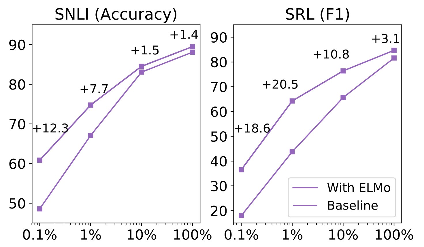
Figure 1: Comparison of baseline vs. ELMo performance for SNLI and SRL as the training set size is varied from 0.1% to 100%.

图 1：当训练集大小从 0.1% 变到 100% 时，SNLI 与 SRL 上基线与 ELMo 表现的比较。

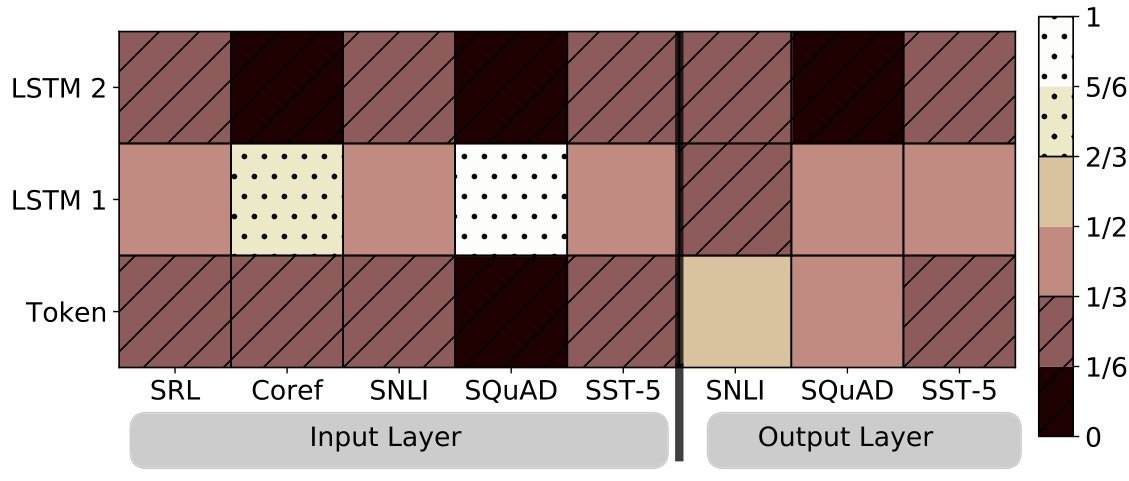
Figure 2: Visualization of softmax normalized biLM layer weights across tasks and ELMo locations. Normalized weights less then $1/3$ are hatched with horizontal lines and those greater then $2/3$ are speckled.

图 2：跨任务与 ELMo 位置的 softmax 归一 biLM 层权重可视化。归一权重小于 $1/3$ 的用水平线阴影标出，大于 $2/3$ 的用斑点标出。

5.4 Sample efficiency

5.4 样本效率

Adding ELMo to a model increases the sample efficiency considerably, both in terms of number of parameter updates to reach state-of-the-art performance and the overall training set size. For example, the SRL model reaches a maximum development F1 after 486 epochs of training without ELMo. After adding ELMo, the model exceeds the baseline maximum at epoch 10, a 98% relative decrease in the number of updates needed to reach the same level of performance.

把 ELMo 加入模型会显著提高样本效率，无论是达到当时最优表现所需的参数更新次数，还是整体训练集大小。例如，不含 ELMo 时 SRL 模型在训练 486 个 epoch 后达到最高开发集 F1。加入 ELMo 后，模型在第 10 个 epoch 就超过基线最高值，达到同等表现水平所需更新次数相对减少 98%。

In addition, ELMo-enhanced models use smaller training sets more efficiently than models without ELMo. Figure 1 compares the performance of baselines models with and without ELMo as the percentage of the full training set is varied from 0.1% to 100%. Improvements with ELMo are largest for smaller training sets and significantly reduce the amount of training data needed to reach a given level of performance. In the SRL case, the ELMo model with 1% of the training set has about the same F1 as the baseline model with 10% of the training set.

此外，ELMo 增强模型比不含 ELMo 的模型更高效地利用较小训练集。图 1 比较了有无 ELMo 时基线模型在完整训练集比例从 0.1% 到 100% 变化时的表现。ELMo 带来的提升在较小训练集上最大，并显著减少达到给定表现水平所需的训练数据量。在 SRL 情形下，使用 1% 训练集的 ELMo 模型与使用 10% 训练集的基线模型 F1 大致相当。

5.5 Visualization of learned weights

5.5 学到权重的可视化

Figure 2 visualizes the softmax-normalized learned layer weights. At the input layer, the task model favors the first biLSTM layer. For coreference and SQuAD, the this is strongly favored, but the distribution is less peaked for the other tasks. The output layer weights are relatively balanced, with a slight preference for the lower layers.

图 2 可视化经 softmax 归一的学到层权重。在输入层，任务模型偏好第一层 biLSTM。对核心指代与 SQuAD，这一偏好很强；对其余任务，分布不那么尖锐。输出层权重相对均衡，对较低层略有偏好。

6 Conclusion

6 结论

We have introduced a general approach for learning high-quality deep context-dependent representations from biLMs, and shown large improvements when applying ELMo to a broad range of NLP tasks. Through ablations and other controlled experiments, we have also confirmed that the biLM layers efficiently encode different types of syntactic and semantic information about words-in-context, and that using all layers improves overall task performance.

我们提出了一种从 biLM 学习高质量、深度、依赖上下文表示的通用方法，并表明把 ELMo 应用到广泛 NLP 任务时可获得大幅提升。通过消融与其他受控实验，我们还证实 biLM 各层高效编码关于上下文中词的不同类型句法与语义信息，并且使用所有层可提升整体任务表现。

References

参考文献

Ba et al. (2016) Jimmy Ba, Ryan Kiros, and Geoffrey E. Hinton. 2016. Layer normalization. CoRR abs/1607.06450.

Belinkov et al. (2017) Yonatan Belinkov, Nadir Durrani, Fahim Dalvi, Hassan Sajjad, and James R. Glass. 2017. What do neural machine translation models learn about morphology? In ACL .

Bojanowski et al. (2017) Piotr Bojanowski, Edouard Grave, Armand Joulin, and Tomas Mikolov. 2017. Enriching word vectors with subword information. TACL 5:135–146.

Bowman et al. (2015) Samuel R. Bowman, Gabor Angeli, Christopher Potts, and Christopher D. Manning. 2015. A large annotated corpus for learning natural language inference. In Proceedings of the 2015 Conference on Empirical Methods in Natural Language Processing (EMNLP) . Association for Computational Linguistics.

Chelba et al. (2014) Ciprian Chelba, Tomas Mikolov, Mike Schuster, Qi Ge, Thorsten Brants, Phillipp Koehn, and Tony Robinson. 2014. One billion word benchmark for measuring progress in statistical language modeling. In INTERSPEECH .

Chen et al. (2017) Qian Chen, Xiao-Dan Zhu, Zhen-Hua Ling, Si Wei, Hui Jiang, and Diana Inkpen. 2017. Enhanced lstm for natural language inference. In ACL .

Chiu and Nichols (2016) Jason Chiu and Eric Nichols. 2016. Named entity recognition with bidirectional LSTM-CNNs. In TACL .

Cho et al. (2014) Kyunghyun Cho, Bart van Merrienboer, Dzmitry Bahdanau, and Yoshua Bengio. 2014. On the properties of neural machine translation: Encoder-decoder approaches. In SSST@EMNLP .

Clark and Gardner (2017) Christopher Clark and Matthew Gardner. 2017. Simple and effective multi-paragraph reading comprehension. CoRR abs/1710.10723.

Clark and Manning (2016) Kevin Clark and Christopher D. Manning. 2016. Deep reinforcement learning for mention-ranking coreference models. In EMNLP .

Collobert et al. (2011) Ronan Collobert, Jason Weston, Léon Bottou, Michael Karlen, Koray Kavukcuoglu, and Pavel P. Kuksa. 2011. Natural language processing (almost) from scratch. In JMLR .

Dai and Le (2015) Andrew M. Dai and Quoc V. Le. 2015. Semi-supervised sequence learning. In NIPS .

Durrett and Klein (2013) Greg Durrett and Dan Klein. 2013. Easy victories and uphill battles in coreference resolution. In EMNLP .

Gal and Ghahramani (2016) Yarin Gal and Zoubin Ghahramani. 2016. A theoretically grounded application of dropout in recurrent neural networks. In NIPS .

Gong et al. (2018) Yichen Gong, Heng Luo, and Jian Zhang. 2018. Natural language inference over interaction space. In ICLR .

Hashimoto et al. (2017) Kazuma Hashimoto, Caiming Xiong, Yoshimasa Tsuruoka, and Richard Socher. 2017. A joint many-task model: Growing a neural network for multiple nlp tasks. In EMNLP 2017 .

He et al. (2017) Luheng He, Kenton Lee, Mike Lewis, and Luke S. Zettlemoyer. 2017. Deep semantic role labeling: What works and what’s next. In ACL .

Hochreiter and Schmidhuber (1997) Sepp Hochreiter and Jürgen Schmidhuber. 1997. Long short-term memory. Neural Computation 9.

Iacobacci et al. (2016) Ignacio Iacobacci, Mohammad Taher Pilehvar, and Roberto Navigli. 2016. Embeddings for word sense disambiguation: An evaluation study. In ACL .

Józefowicz et al. (2016) Rafal Józefowicz, Oriol Vinyals, Mike Schuster, Noam Shazeer, and Yonghui Wu. 2016. Exploring the limits of language modeling. CoRR abs/1602.02410.

Józefowicz et al. (2015) Rafal Józefowicz, Wojciech Zaremba, and Ilya Sutskever. 2015. An empirical exploration of recurrent network architectures. In ICML .

Kim et al. (2015) Yoon Kim, Yacine Jernite, David Sontag, and Alexander M Rush. 2015. Character-aware neural language models. In AAAI 2016 .

Kingma and Ba (2015) Diederik P. Kingma and Jimmy Ba. 2015. Adam: A method for stochastic optimization. In ICLR .

Kumar et al. (2016) Ankit Kumar, Ozan Irsoy, Peter Ondruska, Mohit Iyyer, Ishaan Gulrajani James Bradbury, Victor Zhong, Romain Paulus, and Richard Socher. 2016. Ask me anything: Dynamic memory networks for natural language processing. In ICML .

Lafferty et al. (2001) John D. Lafferty, Andrew McCallum, and Fernando Pereira. 2001. Conditional random fields: Probabilistic models for segmenting and labeling sequence data. In ICML .

Lample et al. (2016) Guillaume Lample, Miguel Ballesteros, Sandeep Subramanian, Kazuya Kawakami, and Chris Dyer. 2016. Neural architectures for named entity recognition. In NAACL-HLT .

Lee et al. (2017) Kenton Lee, Luheng He, Mike Lewis, and Luke S. Zettlemoyer. 2017. End-to-end neural coreference resolution. In EMNLP .

Ling et al. (2015) Wang Ling, Chris Dyer, Alan W. Black, Isabel Trancoso, Ramon Fermandez, Silvio Amir, Luís Marujo, and Tiago Luís. 2015. Finding function in form: Compositional character models for open vocabulary word representation. In EMNLP .

Liu et al. (2017) Xiaodong Liu, Yelong Shen, Kevin Duh, and Jianfeng Gao. 2017. Stochastic answer networks for machine reading comprehension. arXiv preprint arXiv:1712.03556 .

Ma and Hovy (2016) Xuezhe Ma and Eduard H. Hovy. 2016. End-to-end sequence labeling via bi-directional LSTM-CNNs-CRF. In ACL .

Marcus et al. (1993) Mitchell P. Marcus, Beatrice Santorini, and Mary Ann Marcinkiewicz. 1993. Building a large annotated corpus of english: The penn treebank. Computational Linguistics 19:313–330.

McCann et al. (2017) Bryan McCann, James Bradbury, Caiming Xiong, and Richard Socher. 2017. Learned in translation: Contextualized word vectors. In NIPS 2017 .

Melamud et al. (2016) Oren Melamud, Jacob Goldberger, and Ido Dagan. 2016. context2vec: Learning generic context embedding with bidirectional lstm. In CoNLL .

Melis et al. (2017) Gábor Melis, Chris Dyer, and Phil Blunsom. 2017. On the state of the art of evaluation in neural language models. CoRR abs/1707.05589.

Merity et al. (2017) Stephen Merity, Nitish Shirish Keskar, and Richard Socher. 2017. Regularizing and optimizing lstm language models. CoRR abs/1708.02182.

Mikolov et al. (2013) Tomas Mikolov, Ilya Sutskever, Kai Chen, Greg S Corrado, and Jeff Dean. 2013. Distributed representations of words and phrases and their compositionality. In NIPS .

Miller et al. (1994) George A. Miller, Martin Chodorow, Shari Landes, Claudia Leacock, and Robert G. Thomas. 1994. Using a semantic concordance for sense identification. In HLT .

Munkhdalai and Yu (2017) Tsendsuren Munkhdalai and Hong Yu. 2017. Neural tree indexers for text understanding. In EACL .

Neelakantan et al. (2014) Arvind Neelakantan, Jeevan Shankar, Alexandre Passos, and Andrew McCallum. 2014. Efficient non-parametric estimation of multiple embeddings per word in vector space. In EMNLP .

Palmer et al. (2005) Martha Palmer, Paul Kingsbury, and Daniel Gildea. 2005. The proposition bank: An annotated corpus of semantic roles. Computational Linguistics 31:71–106.

Pennington et al. (2014) Jeffrey Pennington, Richard Socher, and Christopher D. Manning. 2014. Glove: Global vectors for word representation. In EMNLP .

Peters et al. (2017) Matthew E. Peters, Waleed Ammar, Chandra Bhagavatula, and Russell Power. 2017. Semi-supervised sequence tagging with bidirectional language models. In ACL .

Pradhan et al. (2013) Sameer Pradhan, Alessandro Moschitti, Nianwen Xue, Hwee Tou Ng, Anders Björkelund, Olga Uryupina, Yuchen Zhang, and Zhi Zhong. 2013. Towards robust linguistic analysis using ontonotes. In CoNLL .

Pradhan et al. (2012) Sameer Pradhan, Alessandro Moschitti, Nianwen Xue, Olga Uryupina, and Yuchen Zhang. 2012. Conll-2012 shared task: Modeling multilingual unrestricted coreference in ontonotes. In EMNLP-CoNLL Shared Task .

Raganato et al. (2017a) Alessandro Raganato, Claudio Delli Bovi, and Roberto Navigli. 2017a. Neural sequence learning models for word sense disambiguation. In EMNLP .

Raganato et al. (2017b) Alessandro Raganato, Jose Camacho-Collados, and Roberto Navigli. 2017b. Word sense disambiguation: A unified evaluation framework and empirical comparison. In EACL .

Rajpurkar et al. (2016) Pranav Rajpurkar, Jian Zhang, Konstantin Lopyrev, and Percy Liang. 2016. Squad: 100, 000+ questions for machine comprehension of text. In EMNLP .

Ramachandran et al. (2017) Prajit Ramachandran, Peter Liu, and Quoc Le. 2017. Improving sequence to sequence learning with unlabeled data. In EMNLP .

Sang and Meulder (2003) Erik F. Tjong Kim Sang and Fien De Meulder. 2003. Introduction to the CoNLL-2003 shared task: Language-independent named entity recognition. In CoNLL .

Seo et al. (2017) Min Joon Seo, Aniruddha Kembhavi, Ali Farhadi, and Hannaneh Hajishirzi. 2017. Bidirectional attention flow for machine comprehension. In ICLR .

Socher et al. (2013) Richard Socher, Alex Perelygin, Jean Y Wu, Jason Chuang, Christopher D Manning, Andrew Y Ng, and Christopher Potts. 2013. Recursive deep models for semantic compositionality over a sentiment treebank. In EMNLP .

Søgaard and Goldberg (2016) Anders Søgaard and Yoav Goldberg. 2016. Deep multi-task learning with low level tasks supervised at lower layers. In ACL 2016 .

Srivastava et al. (2014) Nitish Srivastava, Geoffrey E. Hinton, Alex Krizhevsky, Ilya Sutskever, and Ruslan Salakhutdinov. 2014. Dropout: a simple way to prevent neural networks from overfitting. Journal of Machine Learning Research 15:1929–1958.

Srivastava et al. (2015) Rupesh Kumar Srivastava, Klaus Greff, and Jürgen Schmidhuber. 2015. Training very deep networks. In NIPS .

Turian et al. (2010) Joseph P. Turian, Lev-Arie Ratinov, and Yoshua Bengio. 2010. Word representations: A simple and general method for semi-supervised learning. In ACL .

Wang et al. (2017) Wenhui Wang, Nan Yang, Furu Wei, Baobao Chang, and Ming Zhou. 2017. Gated self-matching networks for reading comprehension and question answering. In ACL .

Wieting et al. (2016) John Wieting, Mohit Bansal, Kevin Gimpel, and Karen Livescu. 2016. Charagram: Embedding words and sentences via character n-grams. In EMNLP .

Wiseman et al. (2016) Sam Wiseman, Alexander M. Rush, and Stuart M. Shieber. 2016. Learning global features for coreference resolution. In HLT-NAACL .

Zeiler (2012) Matthew D. Zeiler. 2012. Adadelta: An adaptive learning rate method. CoRR abs/1212.5701.

Zhou and Xu (2015) Jie Zhou and Wei Xu. 2015. End-to-end learning of semantic role labeling using recurrent neural networks. In ACL .

Zhou et al. (2016) Peng Zhou, Zhenyu Qi, Suncong Zheng, Jiaming Xu, Hongyun Bao, and Bo Xu. 2016. Text classification improved by integrating bidirectional lstm with two-dimensional max pooling. In COLING .

Appendix A Supplemental Material to accompany Deep contextualized word representations

附录 A 伴随 Deep contextualized word representations 的补充材料

This supplement contains details of the model architectures, training routines and hyper-parameter choices for the state-of-the-art models in Section 4.

本补充材料包含第 4 节中当时最优模型的架构、训练流程与超参数选择细节。

All of the individual models share a common architecture in the lowest layers with a context independent token representation below several layers of stacked RNNs – LSTMs in every case except the SQuAD model that uses GRUs.

所有单个模型在最底层共享共性架构：与上下文无关的 token 表示之上堆叠若干层 RNN——除使用 GRU 的 SQuAD 模型外，其余情形均为 LSTM。

A.1 Fine tuning biLM

A.1 微调 biLM

As noted in Sec. 3.4, fine tuning the biLM on task specific data typically resulted in significant drops in perplexity. To fine tune on a given task, the supervised labels were temporarily ignored, the biLM fine tuned for one epoch on the training split and evaluated on the development split. Once fine tuned, the biLM weights were fixed during task training.

如第 3.4 节所述，在任务特定数据上微调 biLM 通常会显著降低困惑度。为在给定任务上微调，暂时忽略有监督标签，在训练划分上对 biLM 微调一个 epoch，并在开发划分上评估。微调完成后，在任务训练期间固定 biLM 权重。

Table 7 lists the development set perplexities for the considered tasks. In every case except CoNLL 2012, fine tuning results in a large improvement in perplexity, e.g., from 72.1 to 16.8 for SNLI.

表 7 列出所考察任务的开发集困惑度。除 CoNLL 2012 外，每一情形下微调都带来大幅困惑度改进，例如 SNLI 从 72.1 降到 16.8。

The impact of fine tuning on supervised performance is task dependent. In the case of SNLI, fine tuning the biLM increased development accuracy 0.6% from 88.9% to 89.5% for our single best model. However, for sentiment classification development set accuracy is approximately the same regardless whether a fine tuned biLM was used.

微调对有监督表现的影响因任务而异。对 SNLI，微调 biLM 把我们单一最佳模型的开发集准确率从 88.9% 提高 0.6% 到 89.5%。然而对情感分类，无论是否使用微调 biLM，开发集准确率大致相同。

A.2 Importance of $\gamma$ in Eqn. (1)

A.2 式 (1) 中 $\gamma$ 的重要性

The $\gamma$ parameter in Eqn. (1) was of practical importance to aid optimization, due to the different distributions between the biLM internal representations and the task specific representations. It is especially important in the last-only case in Sec. 5.1. Without this parameter, the last-only case performed poorly (well below the baseline) for SNLI and training failed completely for SRL.

式 (1) 中的 $\gamma$ 参数对辅助优化具有实际重要性，因为 biLM 内部表示与任务特定表示的分布不同。它在第 5.1 节仅最后一层的情形中尤其重要。若没有该参数，仅最后一层情形在 SNLI 上表现很差（远低于基线），在 SRL 上训练则完全失败。

A.3 Textual Entailment

A.3 文本蕴含

Our baseline SNLI model is the ESIM sequence model from Chen et al. 2017. Following the original implementation, we used 300 dimensions for all LSTM and feed forward layers and pre-trained 300 dimensional GloVe embeddings that were fixed during training. For regularization, we added 50% variational dropout (Gal and Ghahramani 2016) to the input of each LSTM layer and 50% dropout (Srivastava et al. 2014) at the input to the final two fully connected layers. All feed forward layers use ReLU activations. Parameters were optimized using Adam (Kingma and Ba 2015) with gradient norms clipped at 5.0 and initial learning rate 0.0004, decreasing by half each time accuracy on the development set did not increase in subsequent epochs. The batch size was 32.

我们的基线 SNLI 模型是 Chen et al. 2017 的 ESIM 序列模型。按原实现，所有 LSTM 与前馈层使用 300 维，并使用训练期间固定的 300 维预训练 GloVe 嵌入。正则方面，我们在每个 LSTM 层输入处加入 50% 变分 dropout（Gal and Ghahramani 2016），在最后两个全连接层输入处加入 50% dropout（Srivastava et al. 2014）。所有前馈层使用 ReLU 激活。参数用 Adam（Kingma and Ba 2015）优化，梯度范数裁剪为 5.0，初始学习率 0.0004，每当开发集准确率在后续 epoch 不再提升时减半。批量大小为 32。

The best ELMo configuration added ELMo vectors to both the input and output of the lowest layer LSTM, using (1) with layer normalization and $\lambda=0.001$. Due to the increased number of parameters in the ELMo model, we added $\ell^{2}$ regularization with regularization coefficient 0.0001 to all recurrent and feed forward weight matrices and 50% dropout after the attention layer.

最佳 ELMo 配置把 ELMo 向量加到最底层 LSTM 的输入与输出两侧，使用带层归一化的 (1) 且 $\lambda=0.001$。由于 ELMo 模型参数增多，我们对所有循环与前馈权重矩阵加入系数为 0.0001 的 $\ell^{2}$ 正则，并在注意力层后加入 50% dropout。

Table 4 compares test set accuracy of our system to previously published systems. Overall, adding ELMo to the ESIM model improved accuracy by 0.7% establishing a new single model state-of-the-art of 88.7%, and a five member ensemble pushes the overall accuracy to 89.3%.

表 4 比较我们的系统与既往发表系统的测试集准确率。总体而言，把 ELMo 加入 ESIM 模型使准确率提高 0.7%，确立 88.7% 的新单模型当时最优；五成员集成把整体准确率推到 89.3%。

Dataset	Before tuning	Before	tuning	After tuning	After	tuning
Before
tuning
After
tuning
SNLI	72.1	16.8
CoNLL 2012 (coref/SRL)	92.3	-
CoNLL 2003 (NER)	103.2	46.3
SQuAD	Context	99.1	43.5
Questions	158.2	52.0
SST	131.5	78.6

Before
tuning

After
tuning

Table 7: Development set perplexity before and after fine tuning for one epoch on the training set for various datasets (lower is better). Reported values are the average of the forward and backward perplexities.

数据集	微调前	微调后
SNLI	72.1	16.8
CoNLL 2012（coref/SRL）	92.3	-
CoNLL 2003（NER）	103.2	46.3
SQuAD 上下文	99.1	43.5
SQuAD 问题	158.2	52.0
SST	131.5	78.6

表 7：各数据集上在训练集微调一个 epoch 前后的开发集困惑度（越低越好）。报告值为前向与后向困惑度的平均。

Model	Acc.
Feature based (Bowman et al. 2015)	78.2
DIIN (Gong et al. 2018)	88.0
BCN+Char+CoVe (McCann et al. 2017)	88.1
ESIM (Chen et al. 2017)	88.0
ESIM+TreeLSTM (Chen et al. 2017)	88.6
ESIM+ELMo	88.7 $\pm$ 0.17
DIIN ensemble (Gong et al. 2018)	88.9
ESIM+ELMo ensemble	89.3

Table 8: SNLI test set accuracy.[^4]Single model results occupy the portion, with ensemble results at the bottom.

模型	准确率
基于特征（Bowman et al. 2015）	78.2
DIIN（Gong et al. 2018）	88.0
BCN+Char+CoVe（McCann et al. 2017）	88.1
ESIM（Chen et al. 2017）	88.0
ESIM+TreeLSTM（Chen et al. 2017）	88.6
ESIM+ELMo	88.7 $\pm$ 0.17
DIIN 集成（Gong et al. 2018）	88.9
ESIM+ELMo 集成	89.3

表 8：SNLI 测试集准确率。[^4]单模型结果在上半部分，集成结果在底部。

A.4 Question Answering

A.4 问答

Our QA model is a simplified version of the model from Clark and Gardner 2017. It embeds tokens by concatenating each token’s case-sensitive 300 dimensional GloVe word vector (Pennington et al. 2014) with a character-derived embedding produced using a convolutional neural network followed by max-pooling on learned character embeddings. The token embeddings are passed through a shared bi-directional GRU, and then the bi-directional attention mechanism from BiDAF Seo et al. 2017. The augmented context vectors are then passed through a linear layer with ReLU activations, a residual self-attention layer that uses a GRU followed by the same attention mechanism applied context-to-context, and another linear layer with ReLU activations. Finally, the results are fed through linear layers to predict the start and end token of the answer.

我们的 QA 模型是 Clark and Gardner 2017 模型的简化版。它通过拼接每个 token 区分大小写的 300 维 GloVe 词向量（Pennington et al. 2014）与用卷积神经网络再对学习到的字符嵌入做最大池化得到的字符导出嵌入，来嵌入 token。token 嵌入经共享双向 GRU，再经 BiDAF（Seo et al. 2017）的双向注意力机制。增强后的上下文向量再经带 ReLU 激活的线性层、使用 GRU 再接相同注意力机制（上下文对上下文）的残差自注意力层，以及另一带 ReLU 激活的线性层。最后，结果经线性层预测答案的起止 token。

Model	EM	F1
BiDAF (Seo et al. 2017)	68.0	77.3
BiDAF + Self Attention	72.1	81.1
DCN+	75.1	83.1
Reg-RaSoR	75.8	83.3
FusionNet	76.0	83.9
r-net (Wang et al. 2017)	76.5	84.3
SAN (Liu et al. 2017)	76.8	84.4
BiDAF + Self Attention + ELMo	78.6	85.8
DCN+ Ensemble	78.9	86.0
FusionNet Ensemble	79.0	86.0
Interactive AoA Reader+ Ensemble	79.1	86.5
BiDAF + Self Attention + ELMo Ensemble	81.0	87.4

Table 9: Test set results for SQuAD, showing both Exact Match (EM) and F1. The top half of the table contains single model results with ensembles at the bottom. References provided where available.

模型	EM	F1
BiDAF（Seo et al. 2017）	68.0	77.3
BiDAF + Self Attention	72.1	81.1
DCN+	75.1	83.1
Reg-RaSoR	75.8	83.3
FusionNet	76.0	83.9
r-net（Wang et al. 2017）	76.5	84.3
SAN（Liu et al. 2017）	76.8	84.4
BiDAF + Self Attention + ELMo	78.6	85.8
DCN+ 集成	78.9	86.0
FusionNet 集成	79.0	86.0
Interactive AoA Reader+ 集成	79.1	86.5
BiDAF + Self Attention + ELMo 集成	81.0	87.4

表 9：SQuAD 测试集结果，同时给出 Exact Match（EM）与 F1。表上半为单模型结果，底部为集成。在可获得处给出参考文献。

Model	F1
Pradhan et al. 2013	77.5
Zhou and Xu 2015	81.3
He et al. 2017, single	81.7
He et al. 2017, ensemble	83.4
He et al. 2017, our impl.	81.4
He et al. 2017 + ELMo	84.6

Table 10: SRL CoNLL 2012 test set F1.

模型	F1
Pradhan et al. 2013	77.5
Zhou and Xu 2015	81.3
He et al. 2017，单模型	81.7
He et al. 2017，集成	83.4
He et al. 2017，我们的实现	81.4
He et al. 2017 + ELMo	84.6

表 10：SRL CoNLL 2012 测试集 F1。

Variational dropout is used before the input to the GRUs and the linear layers at a rate of 0.2. A dimensionality of 90 is used for the GRUs, and 180 for the linear layers. We optimize the model using Adadelta with a batch size of 45. At test time we use an exponential moving average of the weights and limit the output span to be of at most size 17. We do not update the word vectors during training.

在 GRU 与线性层输入前使用比率为 0.2 的变分 dropout。GRU 维度为 90，线性层为 180。我们用 Adadelta、批量大小 45 优化模型。测试时使用权重的指数滑动平均，并把输出跨度限制为最多 17。训练期间不更新词向量。

Performance was highest when adding ELMo without layer normalization to both the input and output of the contextual GRU layer and leaving the ELMo weights unregularized ($\lambda=0$).

当不加层归一化地把 ELMo 加到上下文 GRU 层的输入与输出两侧、且不对 ELMo 权重正则（$\lambda=0$）时，表现最高。

Table 9 compares test set results from the SQuAD leaderboard as of November 17, 2017 when we submitted our system. Overall, our submission had the highest single model and ensemble results, improving the previous single model result (SAN) by 1.4% F1 and our baseline by 4.2%. A 11 member ensemble pushes F1 to 87.4%, 1.0% increase over the previous ensemble best.

表 9 比较我们于 2017 年 11 月 17 日提交系统时 SQuAD 排行榜的测试集结果。总体而言，我们的提交具有最高的单模型与集成结果，相对既往单模型结果（SAN）提高 1.4% F1，相对我们的基线提高 4.2%。11 成员集成把 F1 推到 87.4%，相对既往集成最佳提高 1.0%。

A.5 Semantic Role Labeling

A.5 语义角色标注

Our baseline SRL model is an exact reimplementation of (He et al. 2017). Words are represented using a concatenation of 100 dimensional vector representations, initialized using GloVe (Pennington et al. 2014) and a binary, per-word predicate feature, represented using an 100 dimensional embedding. This 200 dimensional token representation is then passed through an 8 layer “interleaved” biLSTM with a 300 dimensional hidden size, in which the directions of the LSTM layers alternate per layer. This deep LSTM uses Highway connections (Srivastava et al. 2015) between layers and variational recurrent dropout (Gal and Ghahramani 2016). This deep representation is then projected using a final dense layer followed by a softmax activation to form a distribution over all possible tags. Labels consist of semantic roles from PropBank (Palmer et al. 2005) augmented with a BIO labeling scheme to represent argument spans. During training, we minimize the negative log likelihood of the tag sequence using Adadelta with a learning rate of 1.0 and $\rho=0.95$ (Zeiler 2012). At test time, we perform Viterbi decoding to enforce valid spans using BIO constraints. Variational dropout of 10% is added to all LSTM hidden layers. Gradients are clipped if their value exceeds 1.0. Models are trained for 500 epochs or until validation F1 does not improve for 200 epochs, whichever is sooner. The pretrained GloVe vectors are fine-tuned during training. The final dense layer and all cells of all LSTMs are initialized to be orthogonal. The forget gate bias is initialized to 1 for all LSTMs, with all other gates initialized to 0, as per (Józefowicz et al. 2015).

我们的基线 SRL 模型是对（He et al. 2017）的精确重实现。词用 100 维向量表示的拼接表示，以 GloVe（Pennington et al. 2014）初始化，再加上用 100 维嵌入表示的逐词二元谓词特征。这一 200 维 token 表示再传入隐层大小为 300 的 8 层“交错” biLSTM，其中 LSTM 层方向逐层交替。该深层 LSTM 在层间使用 Highway 连接（Srivastava et al. 2015）以及变分循环 dropout（Gal and Ghahramani 2016）。这一深度表示再经最终稠密层与 softmax 激活投影，形成对所有可能标签的分布。标签由 PropBank（Palmer et al. 2005）的语义角色加上 BIO 标注方案以表示论元跨度组成。训练期间，我们用 Adadelta（学习率 1.0，$\rho=0.95$）（Zeiler 2012）最小化标签序列的负对数似然。测试时做 Viterbi 解码，用 BIO 约束强制有效跨度。所有 LSTM 隐层加入 10% 变分 dropout。若梯度值超过 1.0 则裁剪。模型训练 500 个 epoch，或验证 F1 连续 200 个 epoch 不再提升（以较早者为准）。预训练 GloVe 向量在训练期间微调。最终稠密层与所有 LSTM 的所有单元正交初始化。所有 LSTM 的遗忘门偏置初始化为 1，其余门初始化为 0，按（Józefowicz et al. 2015）。

Table 10 compares test set F1 scores of our ELMo augmented implementation of (He et al. 2017) with previous results. Our single model score of 84.6 F1 represents a new state-of-the-art result on the CONLL 2012 Semantic Role Labeling task, surpassing the previous single model result by 2.9 F1 and a 5-model ensemble by 1.2 F1.

表 10 比较我们的 ELMo 增强版（He et al. 2017）实现与既往结果的测试集 F1。我们 84.6 F1 的单模型分数在 CONLL 2012 语义角色标注任务上确立新的当时最优，超过既往单模型结果 2.9 F1，超过 5 模型集成 1.2 F1。

A.6 Coreference resolution

A.6 核心指代消解

Our baseline coreference model is the end-to-end neural model from Lee et al. 2017 with all hyperparameters exactly following the original implementation.

我们的基线核心指代模型是 Lee et al. 2017 的端到端神经模型，所有超参数完全遵循原实现。

The best configuration added ELMo to the input of the lowest layer biLSTM and weighted the biLM layers using (1) without any regularization ($\lambda=0$) or layer normalization. 50% dropout was added to the ELMo representations.

最佳配置把 ELMo 加到最底层 biLSTM 的输入，并用 (1) 对各 biLM 层加权，不加任何正则（$\lambda=0$）或层归一化。对 ELMo 表示加入 50% dropout。

Table 11 compares our results with previously published results. Overall, we improve the single model state-of-the-art by 3.2% average F1, and our single model result improves the previous ensemble best by 1.6% F1. Adding ELMo to the output from the biLSTM in addition to the biLSTM input reduced F1 by approximately 0.7% (not shown).

表 11 将我们的结果与既往发表结果比较。总体而言，我们把单模型当时最优提高 3.2% 平均 F1，并且我们的单模型结果比既往集成最佳高 1.6% F1。除 biLSTM 输入外再在 biLSTM 输出加入 ELMo，会使 F1 约降 0.7%（未展示）。

Model	Average F1
Durrett and Klein 2013	60.3
Wiseman et al. 2016	64.2
Clark and Manning 2016	65.7
Lee et al. 2017 (single)	67.2
Lee et al. 2017 (ensemble)	68.8
Lee et al. 2017 + ELMo	70.4

Table 11: Coreference resolution average F1 on the test set from the CoNLL 2012 shared task.

模型	平均 F1
Durrett and Klein 2013	60.3
Wiseman et al. 2016	64.2
Clark and Manning 2016	65.7
Lee et al. 2017（单模型）	67.2
Lee et al. 2017（集成）	68.8
Lee et al. 2017 + ELMo	70.4

表 11：CoNLL 2012 共享任务测试集上的核心指代消解平均 F1。

A.7 Named Entity Recognition

A.7 命名实体识别

Our baseline NER model concatenates 50 dimensional pre-trained Senna vectors (Collobert et al. 2011) with a CNN character based representation. The character representation uses 16 dimensional character embeddings and 128 convolutional filters of width three characters, a ReLU activation and by max pooling. The token representation is passed through two biLSTM layers, the first with 200 hidden units and the second with 100 hidden units before a final dense layer and softmax layer. During training, we use a CRF loss and at test time perform decoding using the Viterbi algorithm while ensuring that the output tag sequence is valid.

我们的基线 NER 模型把 50 维预训练 Senna 向量（Collobert et al. 2011）与基于 CNN 的字符表示拼接。字符表示使用 16 维字符嵌入与 128 个宽度为三字符的卷积滤波器，经 ReLU 激活与最大池化。token 表示传入两层 biLSTM，第一层 200 隐单元、第二层 100 隐单元，再接最终稠密层与 softmax 层。训练时使用 CRF 损失，测试时用 Viterbi 算法解码，并确保输出标签序列有效。

Variational dropout is added to the input of both biLSTM layers. During training the gradients are rescaled if their $\ell^{2}$ norm exceeds 5.0 and parameters updated using Adam with constant learning rate of 0.001. The pre-trained Senna embeddings are fine tuned during training. We employ early stopping on the development set and report the averaged test set score across five runs with different random seeds.

在两层 biLSTM 的输入处加入变分 dropout。训练期间若梯度 $\ell^{2}$ 范数超过 5.0 则重新缩放，并用学习率恒为 0.001 的 Adam 更新参数。预训练 Senna 嵌入在训练期间微调。我们在开发集上早停，并报告五个不同随机种子运行的平均测试集分数。

ELMo was added to the input of the lowest layer task biLSTM. As the CoNLL 2003 NER data set is relatively small, we found the best performance by constraining the trainable layer weights to be effectively constant by setting $\lambda=0.1$ with (1).

ELMo 被加到最底层任务 biLSTM 的输入。由于 CoNLL 2003 NER 数据集相对较小，我们发现通过设 $\lambda=0.1$ 并用 (1) 有效约束可训练层权重接近常数时表现最佳。

Table 12 compares test set F1 scores of our ELMo enhanced biLSTM-CRF tagger with previous results. Overall, the 92.22% F1 from our system establishes a new state-of-the-art. When compared to Peters et al. 2017, using representations from all layers of the biLM provides a modest improvement.

表 12 比较我们的 ELMo 增强 biLSTM-CRF 标注器与既往结果的测试集 F1。总体而言，我们系统的 92.22% F1 确立新的当时最优。相对 Peters et al. 2017，使用 biLM 所有层的表示带来适度提升。

Model	F1 $\pm$ std.
Collobert et al. 2011♣	89.59
Lample et al. 2016	90.94
Ma and Hovy 2016	91.2
Chiu and Nichols 2016*♣,♢*	91.62 $\pm$ 0.33
Peters et al. 2017♢	91.93 $\pm$ 0.19
biLSTM-CRF + ELMo	92.22 $\pm$ 0.10

Table 12: Test set F1 for CoNLL 2003 NER task. Models with ♣ included gazetteers and those with ♢ used both the train and development splits for training.

模型	F1 $\pm$ std.
Collobert et al. 2011♣	89.59
Lample et al. 2016	90.94
Ma and Hovy 2016	91.2
Chiu and Nichols 2016*♣,♢*	91.62 $\pm$ 0.33
Peters et al. 2017♢	91.93 $\pm$ 0.19
biLSTM-CRF + ELMo	92.22 $\pm$ 0.10

表 12：CoNLL 2003 NER 任务测试集 F1。带 ♣ 的模型包含地名词典，带 ♢ 的模型同时使用训练与开发划分进行训练。

A.8 Sentiment classification

A.8 情感分类

We use almost the same biattention classification network architecture described in McCann et al. 2017, with the exception of replacing the final maxout network with a simpler feedforward network composed of two ReLu layers with dropout. A BCN model with a batch-normalized maxout network reached significantly lower validation accuracies in our experiments, although there may be discrepancies between our implementation and that of McCann et al. 2017. To match the CoVe training setup, we only train on phrases that contain four or more tokens. We use 300-d hidden states for the biLSTM and optimize the model parameters with Adam Kingma and Ba 2015 using a learning rate of 0.0001. The trainable biLM layer weights are regularized by $\lambda=0.001$, and we add ELMo to both the input and output of the biLSTM; the output ELMo vectors are computed with a second biLSTM and concatenated to the input.

我们使用与 McCann et al. 2017 描述几乎相同的双向注意力分类网络架构，唯一例外是把最终 maxout 网络替换为由两个带 dropout 的 ReLU 层组成的更简单前馈网络。在我们的实验中，带批归一化 maxout 网络的 BCN 模型验证准确率显著更低，尽管我们的实现与 McCann et al. 2017 可能存在差异。为匹配 CoVe 训练设置，我们只在包含四个或更多 token 的短语上训练。biLSTM 使用 300 维隐状态，并用 Adam（Kingma and Ba 2015）以学习率 0.0001 优化模型参数。可训练 biLM 层权重用 $\lambda=0.001$ 正则，并把 ELMo 加到 biLSTM 的输入与输出两侧；输出侧 ELMo 向量用第二个 biLSTM 计算并拼接到输入。

Model	Acc.
DMN (Kumar et al. 2016)	52.1
LSTM-CNN (Zhou et al. 2016)	52.4
NTI (Munkhdalai and Yu 2017)	53.1
BCN+Char+CoVe (McCann et al. 2017)	53.7
BCN+ELMo	54.7

Table 13: Test set accuracy for SST-5.

模型	准确率
DMN（Kumar et al. 2016）	52.1
LSTM-CNN（Zhou et al. 2016）	52.4
NTI（Munkhdalai and Yu 2017）	53.1
BCN+Char+CoVe（McCann et al. 2017）	53.7
BCN+ELMo	54.7

表 13：SST-5 测试集准确率。