EfficientNet: Rethinking Model Scaling for Convolutional Neural Networks
EfficientNet: Rethinking Model Scaling for Convolutional Neural Networks
EfficientNet:重新思考卷积神经网络的模型缩放(EfficientNet: Rethinking Model Scaling for Convolutional Neural Networks)
Mingxing Tan Affiliation: Google Research, Brain Team, Mountain View, CA Correspondence to: tanmingxing@google.com Quoc V. Le Affiliation: Google Research, Brain Team, Mountain View, CA
Abstract
摘要
Convolutional Neural Networks (ConvNets) are commonly developed at a fixed resource budget, and then scaled up for better accuracy if more resources are available. In this paper, we systematically study model scaling and identify that carefully balancing network depth, width, and resolution can lead to better performance. Based on this observation, we propose a new scaling method that uniformly scales all dimensions of depth/width/resolution using a simple yet highly effective compound coefficient. We demonstrate the effectiveness of this method on scaling up MobileNets and ResNet.
卷积神经网络(ConvNet)通常在固定资源预算下设计,再放大以提升精度。缩放的常规做法是加深度或宽度,近年也有提高图像分辨率以换取精度的做法。本文中我们从经验上研究了缩放各维度的过程,发现仔细平衡网络深度、宽度与分辨率可带来更好收益。基于该观察,我们提出一种新的复合缩放方法,用一个简单却高效的复合系数去统一缩放深度、宽度与分辨率。令人惊讶的是,这一系统缩放方法在现有 MobileNet 与 ResNet 上都能轻松提升精度。
To go even further, we use neural architecture search to design a new baseline network and scale it up to obtain a family of models, called EfficientNets, which achieve much better accuracy and efficiency than previous ConvNets. In particular, our EfficientNet-B7 achieves state-of-the-art 84.3% top-1 accuracy on ImageNet, while being 8.4x smaller and 6.1x faster on inference than the best existing ConvNet. Our EfficientNets also transfer well and achieve state-of-the-art accuracy on CIFAR-100 (91.7%), Flowers (98.8%), and 3 other transfer learning datasets, with an order of magnitude fewer parameters. Source code is at https://github.com/tensorflow/tpu/tree/master/models/official/efficientnet.
更进一步,我们用神经架构搜索设计新的基线网络,再放大得到 EfficientNet 模型族;该系列在精度与效率上达到优于此前 ConvNet 的水平。尤其 EfficientNet-B7 在 ImageNet 上达到当时领先的 84.3% top-1 精度,同时比当时最好的 GPipe 小 8.4 倍、推理快 6.1 倍。在常用的迁移学习基准上,EfficientNet 模型同样以少一个数量级的参数量取得当时领先精度。
Keywords:
| Top1 Acc. | #Params | |
|---|---|---|
| ResNet-152 (He et al., 2016) | 77.8% | 60M |
| EfficientNet-B1 | 79.1% | 7.8M |
| ResNeXt-101 (Xie et al., 2017) | 80.9% | 84M |
| EfficientNet-B3 | 81.6% | 12M |
| SENet (Hu et al., 2018) | 82.7% | 146M |
| NASNet-A (Zoph et al., 2018) | 82.7% | 89M |
| EfficientNet-B4 | 82.9% | 19M |
| GPipe (Huang et al., 2018) † | 84.3% | 556M |
| EfficientNet-B7 | 84.3% | 66M |
| †Not plotted |
Figure 1: Model Size vs. ImageNet Accuracy. All numbers are for single-crop, single-model. Our EfficientNets significantly outperform other ConvNets. In particular, EfficientNet-B7 achieves new state-of-the-art 84.3% top-1 accuracy but being 8.4x smaller and 6.1x faster than GPipe. EfficientNet-B1 is 7.6x smaller and 5.7x faster than ResNet-152. Details are in Table 2 and 4.
关键词:
| Top1 Acc. | 参数量 | |
|---|---|---|
| ResNet-152 (He et al., 2016) | 77.8% | 60M |
| EfficientNet-B1 | 79.1% | 7.8M |
| ResNeXt-101 (Xie et al., 2017) | 80.9% | 84M |
| EfficientNet-B3 | 81.6% | 12M |
| SENet (Hu et al., 2018) | 82.7% | 146M |
| NASNet-A (Zoph et al., 2018) | 82.7% | 89M |
| EfficientNet-B4 | 82.9% | 19M |
| GPipe (Huang et al., 2018) † | 84.3% | 556M |
| EfficientNet-B7 | 84.3% | 66M |
| †未绘入图中 |
图 1:模型规模与 ImageNet 精度。 数字均为单裁剪、单模型。EfficientNet 显著优于其他 ConvNet。尤其 EfficientNet-B7 达到当时领先的 84.3% top-1 精度,同时比 GPipe 小 8.4 倍、快 6.1 倍;EfficientNet-B1 比 ResNet-152 小 7.6 倍、快 5.7 倍。细节见表 2 与表 4。
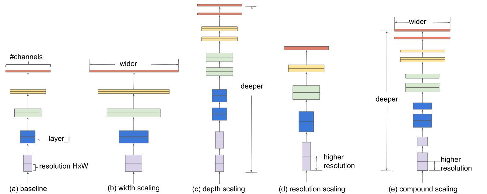
Figure 2: Model Scaling. (a) is a baseline network example; (b)-(d) are conventional scaling that only increases one dimension of network width, depth, or resolution. (e) is our proposed compound scaling method that uniformly scales all three dimensions with a fixed ratio.
图 2:模型缩放。(a)为基线网络示例;(b)–(d)为只增加宽度、深度或分辨率之一的常规缩放;(e)为以固定比例同时统一缩放全部三维的复合缩放方法。
1 Introduction
1 引言
Scaling up ConvNets is widely used to achieve better accuracy. For example, ResNet (He et al., 2016) can be scaled up from ResNet-18 to ResNet-200 by using more layers; Recently, GPipe (Huang et al., 2018) achieved 84.3% ImageNet top-1 accuracy by scaling up a baseline model four time larger. However, the process of scaling up ConvNets has never been well understood and there are currently many ways to do it. The most common way is to scale up ConvNets by their depth (He et al., 2016) or width (Zagoruyko & Komodakis, 2016). Another less common, but increasingly popular, method is to scale up models by image resolution (Huang et al., 2018). In previous work, it is common to scale only one of the three dimensions – depth, width, and image size. Though it is possible to scale two or three dimensions arbitrarily, arbitrary scaling requires tedious manual tuning and still often yields sub-optimal accuracy and efficiency.
扩大ConvNet被广泛用于提高准确性。 例如,ResNet(He等人,2016年)可以通过使用更多的层,从ResNet-18扩大到ResNet-200; 最近,GPipe(Huang等人,2018年)通过提升基线模型4倍大,实现了84.3%的ImageNet顶级-1精度. 然而,ConvNets的扩大进程一直没有得到很好的理解,目前有许多办法可以做到这一点。 最常见的方法是通过深度(He等人,2016年)或宽度(Zagoruyko & Komodakis,2016年)来扩大ConvNets. 另一个不太常见但越来越流行的方法是通过图像分辨率放大模型(Huang等人,2018年). 在之前的作品中,通常只缩放三个维度中的一个——深度,宽度,和图像大小. 虽然可以任意地对两个或三个维度进行测算,但任意测算需要经过繁琐的人工调整,而且仍然往往产生低于最佳的准确性和效率。
In this paper, we want to study and rethink the process of scaling up ConvNets. In particular, we investigate the central question: is there a principled method to scale up ConvNets that can achieve better accuracy and efficiency? Our empirical study shows that it is critical to balance all dimensions of network width/depth/resolution, and surprisingly such balance can be achieved by simply scaling each of them with constant ratio. Based on this observation, we propose a simple yet effective compound scaling method. Unlike conventional practice that arbitrary scales these factors, our method uniformly scales network width, depth, and resolution with a set of fixed scaling coefficients. For example, if we want to use times more computational resources, then we can simply increase the network depth by , width by , and image size by , where are constant coefficients determined by a small grid search on the original small model. Figure 2 illustrates the difference between our scaling method and conventional methods.
在本文中,我们想研究和重新考虑扩大ConvNets的进程. 特别是,我们调查了核心问题:是否有一种原则性的方法来扩大ConvNet,从而能够提高准确性和效率? 我们的实证研究表明,必须平衡网络宽度/深度/分辨率的方方面面,令人惊讶的是,只要以恒定比例来缩小每个层面,就可以实现这种平衡。 基于这一看法,我们提议采用一种简单而有效的*综合缩放方法。 与任意衡量这些因素的常规做法不同,我们的方法统一衡量网络宽度、深度和分辨率,并设定一套固定的衡量系数。 例如,如果我们想要使用比计算资源多一倍,那么我们就可以简单地将网络深度增加,宽度增加,图像大小增加,其中是由在原小模型上小网格搜索确定的恒定系数. 图2显示了我们的缩放方法和传统方法之间的差异。
Intuitively, the compound scaling method makes sense because if the input image is bigger, then the network needs more layers to increase the receptive field and more channels to capture more fine-grained patterns on the bigger image. In fact, previous theoretical (Raghu et al., 2017; Lu et al., 2018) and empirical results (Zagoruyko & Komodakis, 2016) both show that there exists certain relationship between network width and depth, but to our best knowledge, we are the first to empirically quantify the relationship among all three dimensions of network width, depth, and resolution.
直观上,复合缩放法是有道理的,因为如果输入图像更大,那么网络需要更多的层来增加可接受字段和更多的通道来捕捉更大的图像上的更精细的图案. 事实上,之前的理论(Raghu等人,2017年;Lu等人,2018年)和实证结果(Zagoruyko & Komodakis,2016年)都表明网络宽度和深度之间存在一定的关系,但据我们所知,我们是第一个以实证方式量化网络宽度,深度和分辨率所有三个维度之间的关系的.
We demonstrate that our scaling method work well on existing MobileNets (Howard et al., 2017; Sandler et al., 2018) and ResNet (He et al., 2016). Notably, the effectiveness of model scaling heavily depends on the baseline network; to go even further, we use neural architecture search (Zoph & Le, 2017; Tan et al., 2019) to develop a new baseline network, and scale it up to obtain a family of models, called EfficientNets. Figure 1 summarizes the ImageNet performance, where our EfficientNets significantly outperform other ConvNets. In particular, our EfficientNet-B7 surpasses the best existing GPipe accuracy (Huang et al., 2018), but using 8.4x fewer parameters and running 6.1x faster on inference. Compared to the widely used ResNet-50 (He et al., 2016), our EfficientNet-B4 improves the top-1 accuracy from 76.3% to 83.0% (+6.7%) with similar FLOPS. Besides ImageNet, EfficientNets also transfer well and achieve state-of-the-art accuracy on 5 out of 8 widely used datasets, while reducing parameters by up to 21x than existing ConvNets.
我们表明,我们的缩放方法在现有的移动网络(Howard等人,2017年;Sandler等人,2018年)和ResNet(He等人,2016年)上运作良好。 值得注意的是,模型缩放的有效性在很大程度上取决于基线网络;为了更进一步,我们利用神经结构搜索(Zoph & Le, 2017年;Tan等人, 2019年)来开发一个新的基线网络,并扩大其规模,以获得一个被称为“EfficentNets*”的模型家族。 图1总结了ImageNet的性能,我们的高效网络明显优于其他ConvNet。 特别是,我们的高效Net-B7超越了现有最佳的GPipe精度(Huang等人,2018年),但使用了8.4x更少的参数,并在推理上运行了6.1x更快. 与广泛使用的ResNet-50(He等人,2016年)相比,我们的高效Net-B4将具有类似FLOPS的顶级-1精度从76.3%提高到83.0%(+6.7%). 除了ImageNet之外,效率网还很好地传输,并在8个广泛使用的数据集中的5个数据集上实现最先进的精度,同时比现有的ConvNet减少最多21x的参数.
2 Related Work
2 相关工作
ConvNet Accuracy:
Since AlexNet (Krizhevsky et al., 2012) won the 2012 ImageNet competition, ConvNets have become increasingly more accurate by going bigger: while the 2014 ImageNet winner GoogleNet (Szegedy et al., 2015) achieves 74.8% top-1 accuracy with about 6.8M parameters, the 2017 ImageNet winner SENet (Hu et al., 2018) achieves 82.7% top-1 accuracy with 145M parameters. Recently, GPipe (Huang et al., 2018) further pushes the state-of-the-art ImageNet top-1 validation accuracy to 84.3% using 557M parameters: it is so big that it can only be trained with a specialized pipeline parallelism library by partitioning the network and spreading each part to a different accelerator. While these models are mainly designed for ImageNet, recent studies have shown better ImageNet models also perform better across a variety of transfer learning datasets (Kornblith et al., 2019), and other computer vision tasks such as object detection (He et al., 2016; Tan et al., 2019). Although higher accuracy is critical for many applications, we have already hit the hardware memory limit, and thus further accuracy gain needs better efficiency.
ConvNet 精确度 :
自从AlexNet(Krizhevsky等人,2012年)赢得2012年的ImageNet比赛以来,ConvNet通过更大规模而变得越来越准确:而2014年的ImageNet赢家GoogleNet(Szegedy等人,2015年)以约6.8M参数达到74.8%的顶级-1精度,2017年的ImageNet赢家SENet(Hu等人,2018年)以145M参数达到82.7%的顶级-1精度. 最近,GPipe(Huang等人,2018年)进一步将最先进的ImageNet顶级-1验证精度推到84.3%,使用557M参数:其体积巨大,只能通过对网络进行分割,将每个部分分散到不同的加速器进行专业的管道平行主义库训练. 虽然这些模型主要是为ImageNet设计的,但最近的研究表明,更好的ImageNet模型在各种转移学习数据集(Kornblith等人,2019年)和其他计算机视觉任务,如物体检测(He等人,2016年;Tan等人,2019年)中也有更好的表现. 虽然更高的精度对于许多应用程序至关重要,但我们已经达到硬件内存极限,因此进一步精度提高需要更高的效率.
ConvNet Efficiency:
Deep ConvNets are often over-parameterized. Model compression (Han et al., 2016; He et al., 2018; Yang et al., 2018) is a common way to reduce model size by trading accuracy for efficiency. As mobile phones become ubiquitous, it is also common to hand-craft efficient mobile-size ConvNets, such as SqueezeNets (Iandola et al., 2016; Gholami et al., 2018), MobileNets (Howard et al., 2017; Sandler et al., 2018), and ShuffleNets (Zhang et al., 2018; Ma et al., 2018). Recently, neural architecture search becomes increasingly popular in designing efficient mobile-size ConvNets (Tan et al., 2019; Cai et al., 2019), and achieves even better efficiency than hand-crafted mobile ConvNets by extensively tuning the network width, depth, convolution kernel types and sizes. However, it is unclear how to apply these techniques for larger models that have much larger design space and much more expensive tuning cost. In this paper, we aim to study model efficiency for super large ConvNets that surpass state-of-the-art accuracy. To achieve this goal, we resort to model scaling.
ConvNet 效率:
深层ConvNet往往过于参数化. 模型压缩(Han等人,2016年;He等人,2018年;Yang等人,2018年)是通过交易精度以提高效率来降低模型大小的一种常见方式. 随着手机变得无处不在,也常见于手动高效的手机大小Convnet,如SqueezeNets(Iandola等人,2016年;Gholami等人,2018年),MobileNets(Howard等人,2017年;Sandler等人,2018年)和ShuffleNets(Zhang等人,2018年;Ma等人,2018年). 最近,神经架构搜索在设计高效移动大小的ConvNet(Tan et al., 2019;Cai et al., 2019)中越来越受欢迎,并通过广泛调制网络宽度,深度,内核类型和大小,实现比手动ConvNet更高的效率. 然而,目前还不清楚如何将这些技术应用于设计空间大得多、调制成本高得多的大型模型。 在本文中,我们的目标是研究超大型ConvNet的模型效率,这些模型效率超过了最先进的精确度. 为了实现这一目标,我们采用模型规模。
Model Scaling:
There are many ways to scale a ConvNet for different resource constraints: ResNet (He et al., 2016) can be scaled down (e.g., ResNet-18) or up (e.g., ResNet-200) by adjusting network depth (#layers), while WideResNet (Zagoruyko & Komodakis, 2016) and MobileNets (Howard et al., 2017) can be scaled by network width (#channels). It is also well-recognized that bigger input image size will help accuracy with the overhead of more FLOPS. Although prior studies (Raghu et al., 2017; Lin & Jegelka, 2018; Sharir & Shashua, 2018; Lu et al., 2018) have shown that network depth and width are both important for ConvNets’ expressive power, it still remains an open question of how to effectively scale a ConvNet to achieve better efficiency and accuracy. Our work systematically and empirically studies ConvNet scaling for all three dimensions of network width, depth, and resolutions.
- 模型缩放 :
针对 你觉得不同的资源限制,可以有许多方式来扩大一个ConvNet:ResNet(He等人,2016年)可以通过调整网络深度(#layers)来缩小(例如ResNet-18)或上调(例如ResNet-200),而WideResNet(Zagoruyko & Komodakis,2016年)和MobileNet(Howard等人,2017年)可以通过网络宽度(#channels)来缩小. 人们也普遍认识到,更大的输入图像尺寸将有助于准确处理更多FLOPS的间接费用。 虽然之前的研究(Raghu等人,2017年;Lin & Jegelka,2018年;Sharir & Shashua,2018年;Lu等人,2018年)已经表明网络深度和宽度对ConvNets的表达力都很重要,但对于如何有效规模化ConvNet以达到更高的效率和准确性,这仍然是一个尚未解决的问题. 我们的工作对ConvNet在网络宽度、深度和分辨率等所有三个层面的规模进行系统和实证的研究。
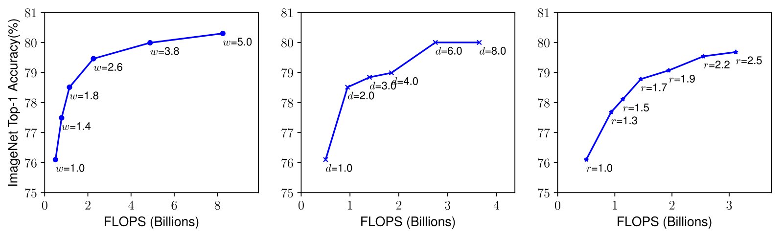
Figure 3: Scaling Up a Baseline Model with Different Network Width (), Depth (), and Resolution () Coefficients. Bigger networks with larger width, depth, or resolution tend to achieve higher accuracy, but the accuracy gain quickly saturate after reaching 80%, demonstrating the limitation of single dimension scaling. Baseline network is described in Table 1.
图3:** 用不同的网络宽度()、深度()和分辨率()扩大基线模型。 ** 宽度,深度或分辨率较大的网络往往能达到更高的精度,但精度在达到80%后迅速饱和,显示了单维缩放的局限性. 基线网络见表1。
3 Compound Model Scaling
3 复合模型缩放
In this section, we will formulate the scaling problem, study different approaches, and propose our new scaling method.
在本节中,我们将提出比例问题,研究不同的办法,并提出新的比例方法。
3.1 Problem Formulation
3.1 问题表述
A ConvNet Layer can be defined as a function: , where is the operator, is output tensor, is input tensor, with tensor shape [^1], where and are spatial dimension and is the channel dimension. A ConvNet can be represented by a list of composed layers: . In practice, ConvNet layers are often partitioned into multiple stages and all layers in each stage share the same architecture: for example, ResNet (He et al., 2016) has five stages, and all layers in each stage has the same convolutional type except the first layer performs down-sampling. Therefore, we can define a ConvNet as:
一个ConvNet Layle 可以定义为函数: ,其中为操作器,为输出拉伸,为输入拉伸,其中拉伸形状为 [^1],其中和为空间维度,为通道维度. 一个ConvNet 可以由组成的层列表来代表: . 在实务中,ConvNet层常被分割成多个阶段,每个阶段的所有层都共享相同的架构:例如ResNet(He等人,2016年)有五个阶段,每个阶段的所有层都有相同的演化类型,除了第一层进行下采样. 因此,我们可以将ConvNet定义为:
where denotes layer is repeated times in stage , denotes the shape of input tensor of layer . Figure 2(a) illustrate a representative ConvNet, where the spatial dimension is gradually shrunk but the channel dimension is expanded over layers, for example, from initial input shape to final output shape .
其中表示第XXMAT 没关系 在阶段重复的,表示第层的输入式成形器 的形状. 图2(a)说明一个具有代表性的ConvNet,空间维度在逐渐缩小,但通道维度在层上扩大,例如从初始输入式的到最终输出式的.
Unlike regular ConvNet designs that mostly focus on finding the best layer architecture , model scaling tries to expand the network length (), width (), and/or resolution () without changing predefined in the baseline network. By fixing , model scaling simplifies the design problem for new resource constraints, but it still remains a large design space to explore different for each layer. In order to further reduce the design space, we restrict that all layers must be scaled uniformly with constant ratio. Our target is to maximize the model accuracy for any given resource constraints, which can be formulated as an optimization problem:
与通常的ConvNet设计大多侧重于寻找最佳层架构不同,模型缩放试图扩展网络长度(),宽度(),和/或分辨率(),而不改变基线网络中预先定义的. 通过修复,模型缩放简化了新资源限制的设计问题,但仍是一个很大的设计空间,用于探索每层不同的. 为了进一步缩小设计空间,我们限制所有层都必须与恒定比例统一缩放. 我们的目标是使模型的准确性最大化,以应对任何特定的资源限制,这可作为一个优化问题:
where are coefficients for scaling network width, depth, and resolution; are predefined parameters in baseline network (see Table 1 as an example).
其中是用于放大网络宽度,深度和分辨率的系数; 是基线网络中预先定义的参数(例见表1).
3.2 Scaling Dimensions
3.2 缩放维度
The main difficulty of problem 2 is that the optimal depend on each other and the values change under different resource constraints. Due to this difficulty, conventional methods mostly scale ConvNets in one of these dimensions:
问题快点,问题2的主要困难在于,最佳的是互相依赖的,价值在不同的资源限制下会发生变化. 由于这一困难,传统方法主要在其中一个方面对ConvNet进行规模化:
Depth ():
Scaling network depth is the most common way used by many ConvNets (He et al., 2016; Huang et al., 2017; Szegedy et al., 2015; Szegedy et al., 2016). The intuition is that deeper ConvNet can capture richer and more complex features, and generalize well on new tasks. However, deeper networks are also more difficult to train due to the vanishing gradient problem (Zagoruyko & Komodakis, 2016). Although several techniques, such as skip connections (He et al., 2016) and batch normalization (Ioffe & Szegedy, 2015), alleviate the training problem, the accuracy gain of very deep network diminishes: for example, ResNet-1000 has similar accuracy as ResNet-101 even though it has much more layers. Figure 3 (middle) shows our empirical study on scaling a baseline model with different depth coefficient , further suggesting the diminishing accuracy return for very deep ConvNets.
桦树():
放大网络深度是许多ConvNet使用的最常见的方式(He等人,2016年;Huang等人,2017年;Szegedy等人,2015年;Szegedy等人,2016年). 直觉是,更深入的ConvNet能够捕捉更丰富和更复杂的特征,并很好地概括新任务. 然而,由于梯度问题消失(Zagoruyko & Komodakis, 2016),更深层的网络也更难训练. 虽然跳过连接(He等人,2016年)和批归一化(Ioffe & Szegedy,2015年)等几种技术缓解了训练问题,但非常深的网络的精度收益却在减弱:例如,ResNet-1000的精度与ResNet-101相似,尽管其分层要多得多. 图3(中)显示了我们对以不同深度系数衡量基准模型的经验性研究,进一步表明非常深的ConvNets的准确性回报率正在下降。
Width ():
Scaling network width is commonly used for small size models (Howard et al., 2017; Sandler et al., 2018; Tan et al., 2019)[^2]. As discussed in (Zagoruyko & Komodakis, 2016), wider networks tend to be able to capture more fine-grained features and are easier to train. However, extremely wide but shallow networks tend to have difficulties in capturing higher level features. Our empirical results in Figure 3 (left) show that the accuracy quickly saturates when networks become much wider with larger .
宽度():
缩放网络宽度通常用于小型模型(Howard等人,2017年;Sandler等人,2018年;Tan等人,2019年)[^2]. 如(Zagoruyko & Komodakis,2016年)所述,较宽的网络往往能够捕捉到更多精细的特征,更容易训练. 然而,极广但很浅的网络往往难以捕捉到更高层次的特征。 我们在图3(左)中的经验结果表明,当网络随着更大的而变得广泛得多时,精度迅速饱和。
Resolution ():
With higher resolution input images, ConvNets can potentially capture more fine-grained patterns. Starting from 224x224 in early ConvNets, modern ConvNets tend to use 299x299 (Szegedy et al., 2016) or 331x331 (Zoph et al., 2018) for better accuracy. Recently, GPipe (Huang et al., 2018) achieves state-of-the-art ImageNet accuracy with 480x480 resolution. Higher resolutions, such as 600x600, are also widely used in object detection ConvNets (He et al., 2017; Lin et al., 2017). Figure 3 (right) shows the results of scaling network resolutions, where indeed higher resolutions improve accuracy, but the accuracy gain diminishes for very high resolutions ( denotes resolution 224x224 and denotes resolution 560x560).
- 决议():
随着分辨率更高的输入图像,ConvNets可能捕捉到更多精细的图案. 从早期ConvNets的224x224开始,现代ConvNets往往使用299x299(Szegedy等人,2016年)或331x331(Zoph等人,2018年)来提高精度. 最近,GPipe(Huang等人,2018年)以480x480的分辨率实现了最先进的ImageNet精度. 600x600等更高分辨率也广泛用于对象检测ConvNets(He等人,2017年;Lin等人,2017年). 图3(右)显示的是比例化网络分辨率的结果,其中高分辨率确实提高了准确度,但非常高分辨率的准确度增益减少(表示224x224号决议,表示560x560号决议)。
The above analyses lead us to the first observation:
上述分析使我们得出第一点看法:
Observation 1 –
Scaling up any dimension of network width, depth, or resolution improves accuracy, but the accuracy gain diminishes for bigger models.
意见1 -
扩大网络宽度、深度或分辨率的任意维度可以提高准确性,但对于更大的模型而言,准确性提高会减少。
3.3 Compound Scaling
3.3 复合缩放
We empirically observe that different scaling dimensions are not independent. Intuitively, for higher resolution images, we should increase network depth, such that the larger receptive fields can help capture similar features that include more pixels in bigger images. Correspondingly, we should also increase network width when resolution is higher, in order to capture more fine-grained patterns with more pixels in high resolution images. These intuitions suggest that we need to coordinate and balance different scaling dimensions rather than conventional single-dimension scaling.
我们从经验上观察到,不同的规模层面并不独立。 直观地,对于更高的分辨率图像,我们应该增加网络深度,这样更大的可接受字段可以帮助捕捉到在更大的图像中包含更多像素的类似特性. 相应地,当分辨率较高时,我们也应该增加网络宽度,以便捕捉高分辨率图像中带有更多像素的更细纹图案. 这些直觉表明,我们需要协调和平衡不同的规模维度,而不是常规的单层规模。
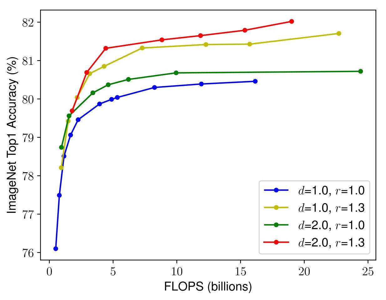
Figure 4: Scaling Network Width for Different Baseline Networks. Each dot in a line denotes a model with different width coefficient (). All baseline networks are from Table 1. The first baseline network (=1.0, =1.0) has 18 convolutional layers with resolution 224x224, while the last baseline (=2.0, =1.3) has 36 layers with resolution 299x299.
图4:不同基线网络的伸缩网络宽度。 一行中的每个点都可持续发展问题表示一个具有不同宽度系数的模型( )。 所有基线网络均来自表1。 第一个基线网络( = 1.0, = 1.0)有18个带有224x224分辨率的卷积层,而最后一个基线( = 2.0, = 1.3)有36个带有299x299分辨率的卷积层.
To validate our intuitions, we compare width scaling under different network depths and resolutions, as shown in Figure 4. If we only scale network width without changing depth (=1.0) and resolution (=1.0), the accuracy saturates quickly. With deeper (=2.0) and higher resolution (=2.0), width scaling achieves much better accuracy under the same FLOPS cost. These results lead us to the second observation:
为了验证我们的直觉,我们比较不同网络深度和分辨率下的宽度缩放,如图4所示. 如果我们在不改变深度( = 1.0)和分辨率( = 1.0)的情况下只缩放网络宽度,精度迅速饱和. 在深度( =2.0)和分辨率较高( =2.0)的情况下,宽度缩放在相同的FLOPS成本下能实现更好的精度. 这些结果使我们得出了第二项意见:
Observation 2 –
In order to pursue better accuracy and efficiency, it is critical to balance all dimensions of network width, depth, and resolution during ConvNet scaling.
意见2 -
为了追求更好的准确性和效率,必须在ConvNet缩放期间平衡网络宽度、深度和分辨率的方方面面。
In fact, a few prior work (Zoph et al., 2018; Real et al., 2019) have already tried to arbitrarily balance network width and depth, but they all require tedious manual tuning.
事实上,之前的几部作品(Zoph et al., 2018;Real et al., 2019)已经尝试任意平衡网络宽度和深度,但它们都要求使用乏味的手动调理.
In this paper, we propose a new compound scaling method, which use a compound coefficient to uniformly scales network width, depth, and resolution in a principled way:
在本文中,我们提议采用新的综合缩放方法,使用复合系数,以原则方式统一缩放网络宽度、深度和分辨率:
where are constants that can be determined by a small grid search. Intuitively, is a user-specified coefficient that controls how many more resources are available for model scaling, while specify how to assign these extra resources to network width, depth, and resolution respectively. Notably, the FLOPS of a regular convolution op is proportional to , , , i.e., doubling network depth will double FLOPS, but doubling network width or resolution will increase FLOPS by four times. Since convolution ops usually dominate the computation cost in ConvNets, scaling a ConvNet with equation 3 will approximately increase total FLOPS by . In this paper, we constraint such that for any new , the total FLOPS will approximately[^3] increase by .
其中是常数,可以通过小网格搜索确定. 直观上,是一个用户指定的系数,它控制了有多少可供模型缩放的资源,而则指定了如何分别将这些额外的资源分配给网络宽度,深度和分辨率. 值得注意的是,常规演化操作的FLOPS与,,成正比,即翻倍的网络深度将翻倍FLOPS,但翻倍的网络宽度或分辨率将翻四倍的FLOPS. 由于ConvNets的计算成本通常以ConvNet为主,使用方程式3的ConvNet的缩放将大约将FLOPS总量增加. 在本文件中,我们对的限制是,对于任何新的,FLOPS总量将增加约[^3] 。
4 EfficientNet Architecture
4 EfficientNet 架构
Since model scaling does not change layer operators in baseline network, having a good baseline network is also critical. We will evaluate our scaling method using existing ConvNets, but in order to better demonstrate the effectiveness of our scaling method, we have also developed a new mobile-size baseline, called EfficientNet.
由于模型缩放不会改变基线网络中的层操作员,因此拥有良好的基线网络也是至关重要的. 我们将利用现有的ConvNet来评估我们的缩放方法,但为了更好地展示我们的缩放方法的有效性,我们还开发了一个新的移动尺寸基线,称为 " 高效率网络 " 。
Inspired by (Tan et al., 2019), we develop our baseline network by leveraging a multi-objective neural architecture search that optimizes both accuracy and FLOPS. Specifically, we use the same search space as (Tan et al., 2019), and use as the optimization goal, where and denote the accuracy and FLOPS of model , is the target FLOPS and =-0.07 is a hyperparameter for controlling the trade-off between accuracy and FLOPS. Unlike (Tan et al., 2019; Cai et al., 2019), here we optimize FLOPS rather than latency since we are not targeting any specific hardware device. Our search produces an efficient network, which we name EfficientNet-B0. Since we use the same search space as (Tan et al., 2019), the architecture is similar to MnasNet, except our EfficientNet-B0 is slightly bigger due to the larger FLOPS target (our FLOPS target is 400M). Table 1 shows the architecture of EfficientNet-B0. Its main building block is mobile inverted bottleneck MBConv (Sandler et al., 2018; Tan et al., 2019), to which we also add squeeze-and-excitation optimization (Hu et al., 2018).
在(Tan等人,2019年)的启发下,我们通过利用多目标神经结构搜索,优化精度和FLOPS,来开发我们的基线网络. 具体而言,我们使用与(Tan等人,2019年)相同的搜索空间,并以作为优化目标,其中和表示型号的准确性和FLOPS,是目标FLOPS, =-0.07是控制精度与FLOPS之间的权衡的超参数. 与(Tan等人,2019年;Cai等人,2019年)不同,我们在这里优化了FLOPS,而不是暂时性,因为我们没有瞄准任何特定的硬件设备. 我们的搜索产生了一个高效的网络,我们称之为 " 高效网-B0 " 。 由于我们使用与(Tan et al.,2019)相同的搜索空间,该架构与MnasNet相似,只是由于FLOPS目标较大(我们的FLOPS目标为400M),我们的高效Net-B0稍大. 表1显示了高效网络-B0的结构。 其主要建筑构件为移动倒转瓶颈MBConv(Sandler等人,2018年;Tan等人,2019年),其中我们还加入了挤压和刺激优化(Hu等人,2018年).
| Stage | Operator | Resolution | #Channels | #Layers |
|---|---|---|---|---|
| 1 | Conv3x3 | 32 | 1 | |
| 2 | MBConv1, k3x3 | 16 | 1 | |
| 3 | MBConv6, k3x3 | 24 | 2 | |
| 4 | MBConv6, k5x5 | 40 | 2 | |
| 5 | MBConv6, k3x3 | 80 | 3 | |
| 6 | MBConv6, k5x5 | 112 | 3 | |
| 7 | MBConv6, k5x5 | 192 | 4 | |
| 8 | MBConv6, k3x3 | 320 | 1 | |
| 9 | Conv1x1 & Pooling & FC | 1280 | 1 |
Table 1: EfficientNet-B0 baseline network– Each row describes a stage with layers, with input resolution and output channels . Notations are adopted from equation 2.
| 阶段 | 运算符 | 决议 | 渠道 | # 骗子们 # |
|---|---|---|---|---|
| 第二十届 | 第二十届 | |||
| 1 | Conv3x3 数据 | 32 | 1 | |
| 2 | MBConv1, k3x3 数据 | 16 | 1 | |
| 3 | MBConv6, k3x3 类型 | 24 | 2 | |
| 4 | MBConv6, k5x5 主题 | 40 | 2 | |
| 5 | MBConv6, k3x3 类型 | 80 | 3 | |
| 6 | MBConv6, k5x5 主题 | 112 | 3 | |
| 7 | MBConv6, k5x5 主题 | 192 | 4 | |
| 8 | MBConv6, k3x3 类型 | 320 | 1 | |
| 9 | Conv1x1 组合 & FC | 1280 | 1 |
表1:** EfficientNet-B0基线网络**** 每行描述一个带有层的阶段,带有输入分辨率和输出通道. 从方程式2中采用注解。
Starting from the baseline EfficientNet-B0, we apply our compound scaling method to scale it up with two steps:
从基线 " 高效网络-B0 " 开始,我们采用复合缩放方法,以两个步骤加以扩大:
- • STEP 1: we first fix , assuming twice more resources available, and do a small grid search of based on Equation 2 and 3. In particular, we find the best values for EfficientNet-B0 are , under constraint of .
- • STEP 2: we then fix as constants and scale up baseline network with different using Equation 3, to obtain EfficientNet-B1 to B7 (Details in Table 2).
- 第1步:我们首先修复,假设可动用的资源增加了两倍,并根据第2和第3款对进行小网格搜索。 特别是,我们发现高效网络-B0的最佳值是,受的限制。
- 步骤2:然后,我们利用第3条方程式将固定为常数,并利用不同的扩大基线网络,以获得高效的Net-B1至B7(详见表2)。
Notably, it is possible to achieve even better performance by searching for directly around a large model, but the search cost becomes prohibitively more expensive on larger models. Our method solves this issue by only doing search once on the small baseline network (step 1), and then use the same scaling coefficients for all other models (step 2).
值得注意的是,通过直接围绕大型模型搜索,可以实现更好的性能,但大型模型的搜索成本却变得昂贵得多。 我们的方法解决了这个问题,只在小型基线网络(步骤1)上进行一次搜索,然后对所有其它模型(步骤2)使用相同的缩放系数.
| Model | Top-1 Acc. | Top-5 Acc. | #Params | Ratio-to-EfficientNet | #FLOPs | Ratio-to-EfficientNet |
|---|---|---|---|---|---|---|
| EfficientNet-B0 | 77.1% | 93.3% | 5.3M | 1x | 0.39B | 1x |
| ResNet-50 (He et al., 2016) | 76.0% | 93.0% | 26M | 4.9x | 4.1B | 11x |
| DenseNet-169 (Huang et al., 2017) | 76.2% | 93.2% | 14M | 2.6x | 3.5B | 8.9x |
| EfficientNet-B1 | 79.1% | 94.4% | 7.8M | 1x | 0.70B | 1x |
| ResNet-152 (He et al., 2016) | 77.8% | 93.8% | 60M | 7.6x | 11B | 16x |
| DenseNet-264 (Huang et al., 2017) | 77.9% | 93.9% | 34M | 4.3x | 6.0B | 8.6x |
| Inception-v3 (Szegedy et al., 2016) | 78.8% | 94.4% | 24M | 3.0x | 5.7B | 8.1x |
| Xception (Chollet, 2017) | 79.0% | 94.5% | 23M | 3.0x | 8.4B | 12x |
| EfficientNet-B2 | 80.1% | 94.9% | 9.2M | 1x | 1.0B | 1x |
| Inception-v4 (Szegedy et al., 2017) | 80.0% | 95.0% | 48M | 5.2x | 13B | 13x |
| Inception-resnet-v2 (Szegedy et al., 2017) | 80.1% | 95.1% | 56M | 6.1x | 13B | 13x |
| EfficientNet-B3 | 81.6% | 95.7% | 12M | 1x | 1.8B | 1x |
| ResNeXt-101 (Xie et al., 2017) | 80.9% | 95.6% | 84M | 7.0x | 32B | 18x |
| PolyNet (Zhang et al., 2017) | 81.3% | 95.8% | 92M | 7.7x | 35B | 19x |
| EfficientNet-B4 | 82.9% | 96.4% | 19M | 1x | 4.2B | 1x |
| SENet (Hu et al., 2018) | 82.7% | 96.2% | 146M | 7.7x | 42B | 10x |
| NASNet-A (Zoph et al., 2018) | 82.7% | 96.2% | 89M | 4.7x | 24B | 5.7x |
| AmoebaNet-A (Real et al., 2019) | 82.8% | 96.1% | 87M | 4.6x | 23B | 5.5x |
| PNASNet (Liu et al., 2018) | 82.9% | 96.2% | 86M | 4.5x | 23B | 6.0x |
| EfficientNet-B5 | 83.6% | 96.7% | 30M | 1x | 9.9B | 1x |
| AmoebaNet-C (Cubuk et al., 2019) | 83.5% | 96.5% | 155M | 5.2x | 41B | 4.1x |
| EfficientNet-B6 | 84.0% | 96.8% | 43M | 1x | 19B | 1x |
| EfficientNet-B7 | 84.3% | 97.0% | 66M | 1x | 37B | 1x |
| GPipe (Huang et al., 2018) | 84.3% | 97.0% | 557M | 8.4x | - | - |
| We omit ensemble and multi-crop models (Hu et al., 2018), or models pretrained on 3.5B Instagram images (Mahajan et al., 2018). |
Table 2: EfficientNet Performance Results on ImageNet (Russakovsky et al., 2015). All EfficientNet models are scaled from our baseline EfficientNet-B0 using different compound coefficient in Equation 3. ConvNets with similar top-1/top-5 accuracy are grouped together for efficiency comparison. Our scaled EfficientNet models consistently reduce parameters and FLOPS by an order of magnitude (up to 8.4x parameter reduction and up to 16x FLOPS reduction) than existing ConvNets.
| 型号 | 顶级1Acc. | 顶-5 Acc. | #Params | 比率与效率网 | #FLOPs | 比率与效率网 |
|---|---|---|---|---|---|---|
| ** EfficientNet-B0** | ** 77.1+++ | **93.3+++ | ** 5.3M ** | 页:1 | 0.39B (单位:千美元) | 页:1 |
| ResNet-50(他等人,2016年) | 76.0% | 93.0% | 26分钟 | 4.9x | 4.1B (韩语) | 11x |
| DenseNet-169 (Huang等人, 2017). | 76.2% | 93.2% | 14分钟 | 2.6x | 3.5B (韩语) | 8.9x |
| ** EfficientNet-B1** | (单位:千美元) | * 94.4% | 7.8M (单位:千美元) | 页:1 | 页:1 | 页:1 |
| ResNet-152(He等人,2016年) | 77.8% | 93.8% | 6万伎俩 | 7.6x | 第11B条 | 16x |
| DenseNet-264 (Huang等人, 2017). | 77.9% | 93.9% | 34分钟 | 4.3x | 6.0B (韩语) | 8.6x |
| Inception-v3(Szegedy等人,2016年) | 78.8% | 94.4% | 24分钟 | 3.0x | 5.7B (韩语) | 8.1x |
| Xception (Chollet, 2017) (英语). | 79.0% | 94.5% | 23分钟 | 3.0x | 8.4B (韩语) | 12x |
| ** EfficientNet-B2** | 快走 | * **94.9++ | ** 9.2M** (单位:千美元) | 页:1 | (单位:千美元) | 页:1 |
| Inception-v4(Szegedy等人,2017年). | 80.0% | 95.0% | 48分钟 | 5.2x | 第13B条 | 13x |
| Inception-resnet-v2(Szegedy等人,2017年). | 80.1% | 95.1% | 5600辆 | 6.1x | 第13B条 | 13x |
| ** EfficientNet-B3** | 页:1 | 页:1 | ** 12M** (单位:千美元) | 页:1 | 页:1 | 页:1 |
| ResNEXt-101(谢等人,2017年). | 80.9% | 95.6% | 84马 | 7.0x | 32B (韩语) | 18x |
| PolyNet(张等,2017). | 81.3% | 95.8% | 92海里 | 7.7x | 35B (韩语) | 19x |
| ** EfficientNet-B4** | 页:1 | 页:1 | 页:1 | 页ان | 页:1 | 页:1 |
| 咀丸(Hu等人,2018年) | 82.7% | 96.2% | 146海里 | 7.7x | 第42B条 | 10x |
| NASNet-A(Zoph等人,2018年) | 82.7% | 96.2% | 89马 | 4.7x | 24个B | 5.7x |
| AmoebaNet-A(Real等人,2019年) | 82.8% | 96.1% | 战利品 | 4.6x | 23B (韩语). | 5.5x |
| PNASNet(Liu等人,2018年) | 82.9% | 96.2% | 86M (英语). | 4.5x | 23B (韩语). | 6.0x |
| ** EfficientNet-B5** | 页:1 | **96.7+++ | 页:1 | 页:1 | (单位:千美元) | 页:1 |
| AmoebaNet-C(Cubuk等人,2019年) | 83.5% | 96.5% | 155M (英语). | 5.2x | 41B (韩语) | 4.1x |
| ** EfficientNet-B6** | 页:1 | **96.8+++ | ** 43M** (单位:千美元) | 页:1 | 页:1 | 页:1 |
| ** EfficientNet-B7** | 页:1 | 页:1 | ** 编号 | 页:1 | 页:1 | 页:1 |
| GPipe(Huang等人,2018年). | 84.3% | 97.0% | 557门 | 8.4x | - | - |
| 我们省略了综艺和多作物模型(Hu等人,2018年),或者在3.5B Instagram图像上预先训练的模型(Mahajan等人,2018年). |
表2:图像网的效能网成绩(Russakovsky等人,2015年)。 所有高效网络模型都从我们的基线 " 高效网络-B0 " 中缩放,使用方程式3中不同的复合系数。 具有类似顶级1/顶级-5精度的ConvNet被归为一组,以进行效率比较. 与现有的ConvNets相比,我们扩大后的高效网络模型将参数和FLOPS不断减少(最多减少8.4x参数,减少16xFLOPS)。
5 Experiments
5 实验
| Model | FLOPS | Top-1 Acc. |
|---|---|---|
| Baseline MobileNetV1 (Howard et al., 2017) | 0.6B | 70.6% |
| Scale MobileNetV1 by width (=2) | 2.2B | 74.2% |
| Scale MobileNetV1 by resolution (=2) | 2.2B | 72.7% |
| compound scale (=1.4, =1.2, =1.3) | 2.3B | 75.6% |
| Baseline MobileNetV2 (Sandler et al., 2018) | 0.3B | 72.0% |
| Scale MobileNetV2 by depth (=4) | 1.2B | 76.8% |
| Scale MobileNetV2 by width (=2) | 1.1B | 76.4% |
| Scale MobileNetV2 by resolution (=2) | 1.2B | 74.8% |
| MobileNetV2 compound scale | 1.3B | 77.4% |
| Baseline ResNet-50 (He et al., 2016) | 4.1B | 76.0% |
| Scale ResNet-50 by depth (=4) | 16.2B | 78.1% |
| Scale ResNet-50 by width (=2) | 14.7B | 77.7% |
| Scale ResNet-50 by resolution (=2) | 16.4B | 77.5% |
| ResNet-50 compound scale | 16.7B | 78.8% |
Table 3: Scaling Up MobileNets and ResNet.
| 型号 | FLOPS | 顶级1Acc. |
|---|---|---|
| 基线移动网络V1(Howard等人,2017年) | 0.6B (韩语) | 70.6% |
| 以宽度缩放移动NetV1(=2) | 2.2B (韩语) | 74.2% |
| 通过决议(=2)缩放移动NetV1 | 2.2B (韩语) | 72.7% |
| ** 缩放(=1.4,=1.2,=1.3)** | 页:1 | ** 75.6 ++ |
| 奠定了基线移动网络V2(Sandler等人,2018年) | 0.3B (韩语) | 72.0% |
| 按深度(=4)缩放 MobileNetV2 | 1.2B (韩语) | 76.8% |
| 以宽度缩放 MobileNetV2 ( = 2) | 1.1B (韩语) | 76.4% |
| 通过分辨率(=2)缩放移动网络V2 | 1.2B (韩语) | 74.8% |
| ** 移动NetV2复合尺度** | 页:1 | ** 77.4+++ |
| ResNet-50基线(他等人,2016年) | 4.1B (韩语) | 76.0% |
| 按深度划分的ResNet-50比例(=4) | 16.2B (韩语). | 78.1% |
| 按宽度划分的ResNet-50(=2) | 14.7B (中文(简体) ). | 77.7% |
| 按决议(=2)调整ResNet-50 | 16‛4B | 77.5% |
| ** ResNet-50复合比额表** | 页:1 | 页:1 |
表3:** 扩大移动网络和ResNet。 **
In this section, we will first evaluate our scaling method on existing ConvNets and the new proposed EfficientNets.
在本节中,我们将首先评估我们在现有ConvNet和新的拟议高效网络上的缩放方法。
5.1 Scaling Up MobileNets and ResNets
5.1 放大 MobileNet 与 ResNet
As a proof of concept, we first apply our scaling method to the widely-used MobileNets (Howard et al., 2017; Sandler et al., 2018) and ResNet (He et al., 2016). Table 3 shows the ImageNet results of scaling them in different ways. Compared to other single-dimension scaling methods, our compound scaling method improves the accuracy on all these models, suggesting the effectiveness of our proposed scaling method for general existing ConvNets.
作为概念的证明,我们首先将我们的缩放方法应用于广泛使用的MobileNets(Howard等人,2017年;Sandler等人,2018年)和ResNet(He等人,2016年). 表3显示图像网络以不同方式加以放大的结果。 与其他单元缩放方法相比,我们的复合缩放方法提高了所有这些模型的准确性,表明我们提议的缩放方法对于一般现有ConvNet的有效性.
| Acc. @ Latency | Acc. @ Latency | ||
|---|---|---|---|
| ResNet-152 | 77.8% @ 0.554s | GPipe | 84.3% @ 19.0s |
| EfficientNet-B1 | 78.8% @ 0.098s | EfficientNet-B7 | 84.4% @ 3.1s |
| Speedup | 5.7x | Speedup | 6.1x |
Table 4: Inference Latency Comparison – Latency is measured with batch size 1 on a single core of Intel Xeon CPU E5-2690.
| 校对:Soup | 校对:Soup | ||
|---|---|---|---|
| ResNet-152号卫星 | 77.8%@ 0.554s (单位:千美元) | 胶片 | 84.3%@ 19.0%s |
| 高效率的通用网络B1 | 78.8% @ 0.098s | 高效网络B7 | 84.4%@3.1s |
| 页:1 | 页:1 | 页:1 | 6.1x (单位:这方面的工作量) |
表4:推理纬度比较 – 在Intel Xeon CPU E5-2690的单个核心上用批量尺寸1测量纬度.
| Top1 Acc. | FLOPS | |
|---|---|---|
| ResNet-152 (Xie et al., 2017) | 77.8% | 11B |
| EfficientNet-B1 | 79.1% | 0.7B |
| ResNeXt-101 (Xie et al., 2017) | 80.9% | 32B |
| EfficientNet-B3 | 81.6% | 1.8B |
| SENet (Hu et al., 2018) | 82.7% | 42B |
| NASNet-A (Zoph et al., 2018) | 80.7% | 24B |
| EfficientNet-B4 | 82.9% | 4.2B |
| AmeobaNet-C (Cubuk et al., 2019) | 83.5% | 41B |
| EfficientNet-B5 | 83.6% | 9.9B |
Figure 5: FLOPS vs. ImageNet Accuracy – Similar to Figure 1 except it compares FLOPS rather than model size.
| Top1 Acc. (中文(简体) ). | FLOPS | |
|---|---|---|
| ResNet-152(谢等人,2017年) | 77.8% | 第11B条 |
| ** 效能网-B1** | * **79.1ĩa | 页:1 |
| ResNEXt-101(谢等人,2017年). | 80.9% | 32B (韩语) |
| ** EfficientNet-B3** | 页:1 | 页:1 |
| SENET(Hu等人,2018年) | 82.7% | 第42B条 |
| NASNet-A(Zoph等人,2018年) | 80.7% | 24个B |
| ** EfficientNet-B4** | 页:1 | 页:1 |
| AmeobaNet-C(Cubuk等人,2019年) | 83.5% | 41B (韩语) |
| ** EfficientNet-B5** | 页:1 | (单位:千美元) |
图5:**FLOPS vs. ImageNet 准确性 与图1相似,只是比较了FLOPS而不是模型大小.
| Comparison to best public-available results | Comparison to best reported results | |||||||||||
|---|---|---|---|---|---|---|---|---|---|---|---|---|
| Model | Acc. | #Param | Our Model | Acc. | #Param(ratio) | Model | Acc. | #Param | Our Model | Acc. | #Param(ratio) | |
| CIFAR-10 | NASNet-A | 98.0% | 85M | EfficientNet-B0 | 98.1% | 4M (21x) | †Gpipe | 99.0% | 556M | EfficientNet-B7 | 98.9% | 64M (8.7x) |
| CIFAR-100 | NASNet-A | 87.5% | 85M | EfficientNet-B0 | 88.1% | 4M (21x) | Gpipe | 91.3% | 556M | EfficientNet-B7 | 91.7% | 64M (8.7x) |
| Birdsnap | Inception-v4 | 81.8% | 41M | EfficientNet-B5 | 82.0% | 28M (1.5x) | GPipe | 83.6% | 556M | EfficientNet-B7 | 84.3% | 64M (8.7x) |
| Stanford Cars | Inception-v4 | 93.4% | 41M | EfficientNet-B3 | 93.6% | 10M (4.1x) | ‡DAT | 94.8% | - | EfficientNet-B7 | 94.7% | - |
| Flowers | Inception-v4 | 98.5% | 41M | EfficientNet-B5 | 98.5% | 28M (1.5x) | DAT | 97.7% | - | EfficientNet-B7 | 98.8% | - |
| FGVC Aircraft | Inception-v4 | 90.9% | 41M | EfficientNet-B3 | 90.7% | 10M (4.1x) | DAT | 92.9% | - | EfficientNet-B7 | 92.9% | - |
| Oxford-IIIT Pets | ResNet-152 | 94.5% | 58M | EfficientNet-B4 | 94.8% | 17M (5.6x) | GPipe | 95.9% | 556M | EfficientNet-B6 | 95.4% | 41M (14x) |
| Food-101 | Inception-v4 | 90.8% | 41M | EfficientNet-B4 | 91.5% | 17M (2.4x) | GPipe | 93.0% | 556M | EfficientNet-B7 | 93.0% | 64M (8.7x) |
| Geo-Mean | (4.7x) | (9.6x) | ||||||||||
| †GPipe (Huang et al., 2018) trains giant models with specialized pipeline parallelism library. | ||||||||||||
| ‡DAT denotes domain adaptive transfer learning (Ngiam et al., 2018). Here we only compare ImageNet-based transfer learning results. | ||||||||||||
| Transfer accuracy and #params for NASNet (Zoph et al., 2018), Inception-v4 (Szegedy et al., 2017), ResNet-152 (He et al., 2016) are from (Kornblith et al., 2019). |
Table 5: EfficientNet Performance Results on Transfer Learning Datasets. Our scaled EfficientNet models achieve new state-of-the-art accuracy for 5 out of 8 datasets, with 9.6x fewer parameters on average.
| 与最佳公共成果的比较 | 与最佳报告结果的比较 | |||||||||||
|---|---|---|---|---|---|---|---|---|---|---|---|---|
| 第 12 条 | Acc. | #Param | 我们的模特儿 | Acc. | #Param(鼠标) | 型号 | Acc. | #Param | 我们的模特儿 | Acc. | #Param(鼠标) | |
| 科伊法尔-10 | 纳斯网- 页:1 | 98.0% | 85分钟 | 高效网络B0 | 98.1% | 4M(21辆) | • 气管 | 99.0% | 556海里 | 高效网络B7 | 98.9% | 64M(8.7x) (中文(简体) ). |
| CIFAR-100 (法语) | 纳斯网- A级 | 87.5% | 85分钟 | 高效网络B0 | 88.1% | 4M(21x) (中文(简体) ). | 气管 | 91.3% | 556海里 | 高效网络B7 | 页:1 | 64M(8.7x) (中文(简体) ). |
| 鸟巢 | 感应V4 | 81.8% | 41分钟 | 高效网络B5 | 82.0% | 28M(1.5x) (中文(简体) ). | 胶片 | 83.6% | 556海里 | 高效网络B7 | 页:1 | 64防止冲突(8.7x) |
| 斯坦福车厢所得到的 | 感应V4 | 93.4% | 41分钟 | 高效网络B3 | 93.6% | 10M(4.1x) 导弹 警察 | 数据 | 页:1 | - | 高效网络B7 | 94.7% | - |
| 鲜花 | 感应V4 | 98.5% | 41分钟 | 高效网络B5 | 98.5% | 28M (1.5x) (中文(简体) ). | 数字 | 97.7% | - | 高效率网络B7 | * 98.8* | - |
| FGVC 飞机 | 感应V4 | 90.9% | 41分钟 | 高效网络B3 | 90.7% | 10M (4.1x) (中文(简体) ). | 数字 | 92.9% | - | 高效网络B7 | **92.9+++ | - |
| 牛津-IIIT 宠物 | ResNet-152号卫星 | 94.5% | 58分钟 | 高效网络-B4 | 94.8% | 17M (5.6x) (中文(简体) ). | 胶片 | 我刚说到 | 556海里 | 高效网络B6 | 95.4% | 41M(14x) (中文(简体) ). |
| 粮食101 | 感应V4 | 90.8% | 41分钟 | 高效网络-B4 | 91.5% | 17门(2.4x) | ip | 93.0% | 556海里 | 高效网络B7 | 页:1 | 64M(8.7x) (中文(简体) ). |
| 地理主题 | (4.7x) (单位:千美元) | ** (9.6x)** (单位:千美元) | ||||||||||
| QQ在国家和国际一级 (Huang et al., 2018) 训练具有专业管道平行主义图书馆的巨型模型. | ||||||||||||
| QQDAT表示域适应性转移学习(Ngiam等人,2018年). 这里我们只比较基于ImageNet的转移学习结果. | ||||||||||||
| NASNet(Zoph等人,2018年)、Inception-v4(Szegedy等人,2017年)、ResNet-152(He等人,2016年)的传输精度和#参数来自(Kornblith等人,2019年)。 |
表5:** 转让学习数据集的EfficientNet络绩效结果**。 我们的扩大的 " 高效网络 " 模型在8个数据集中,有5个实现了新的最新精度,平均减少9.6x参数。
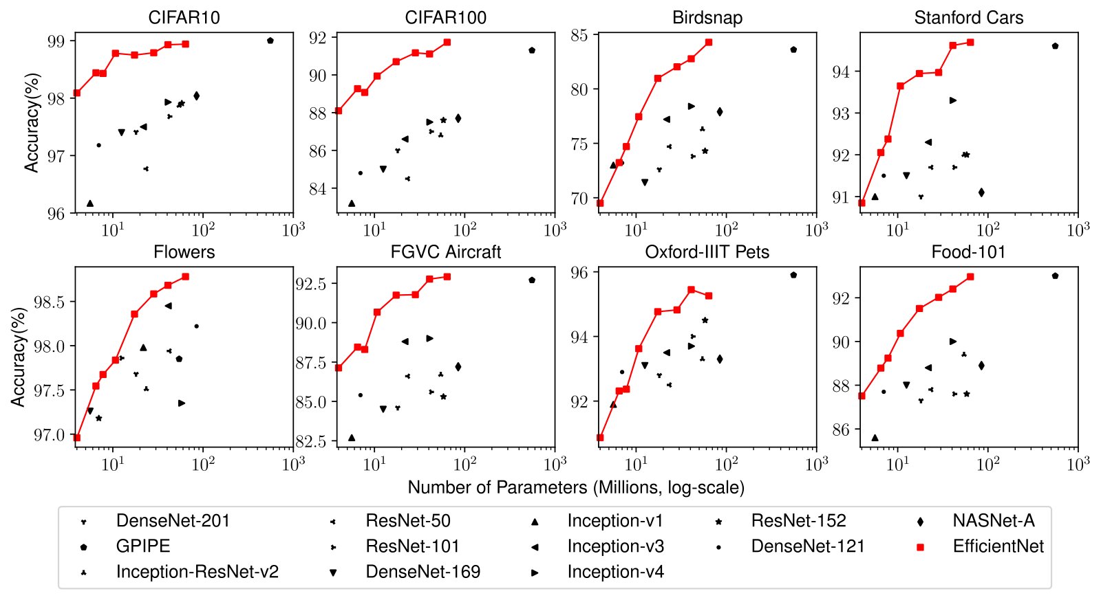
Figure 6: Model Parameters vs. Transfer Learning Accuracy – All models are pretrained on ImageNet and finetuned on new datasets.
ý 校对:Soup 所有模型都预先在ImageNet上训练,并在新的数据集上微调.
5.2 ImageNet Results for EfficientNet
5.2 EfficientNet 的 ImageNet 结果
We train our EfficientNet models on ImageNet using similar settings as (Tan et al., 2019): RMSProp optimizer with decay 0.9 and momentum 0.9; batch norm momentum 0.99; weight decay 1e-5; initial learning rate 0.256 that decays by 0.97 every 2.4 epochs. We also use SiLU (Swish-1) activation (Ramachandran et al., 2018; Elfwing et al., 2018; Hendrycks & Gimpel, 2016), AutoAugment (Cubuk et al., 2019), and stochastic depth (Huang et al., 2016) with survival probability 0.8. As commonly known that bigger models need more regularization, we linearly increase dropout (Srivastava et al., 2014) ratio from 0.2 for EfficientNet-B0 to 0.5 for B7. We reserve 25K randomly picked images from the training set as a minival set, and perform early stopping on this minival; we then evaluate the early-stopped checkpoint on the original validation set to report the final validation accuracy.
我们在ImageNet上使用类似的设置(Tan等人,2019年):RMSProp优化器,衰减0.9和动力0.9;批归一化动力0.99;重量衰减1e-5;初始学习率0.256,每2.4个纪元衰减0.97。 我们还使用SiLU(Swish-1)激活(Ramachandran等人,2018年;Elfwing等人,2018年;Hendrycks & Gimpel,2016年),AutoAugment(Cubuk等人,2019年),以及具有存活概率0.8. 众所周知,较大的模型需要更多的正规化,因此,我们线性地增加了辍学率(Srivastava等人,2014年),从效率网-B0的0.2上升到B7的0.5。 我们保留25K随机从训练集中选取的影像作为迷你瓦片集,并在这个迷你瓦片上进行早期的停放;然后在原始的验证集上评价早期停放的检查点,以报告最终的验证准确性.
Table 2 shows the performance of all EfficientNet models that are scaled from the same baseline EfficientNet-B0. Our EfficientNet models generally use an order of magnitude fewer parameters and FLOPS than other ConvNets with similar accuracy. In particular, our EfficientNet-B7 achieves 84.3% top1 accuracy with 66M parameters and 37B FLOPS, being more accurate but 8.4x smaller than the previous best GPipe (Huang et al., 2018). These gains come from both better architectures, better scaling, and better training settings that are customized for EfficientNet.
表2显示从同一基准的 " 高效率网络 " B0中缩放的所有高效网络模型的性能。 我们的高效网络模型一般比其他精度相似的ConvNet使用数量级的更少参数和FLOPS. 特别是,我们的高效Net-B7在66M参数和37B FLOPS中实现了84.3%的顶级精度,比之前最好的GPipe(Huang等人,2018年)更准确,但8.4x小。 这些收益既来自更好的架构、更好的规模化,也来自为高效网络定制的更好的训练环境。
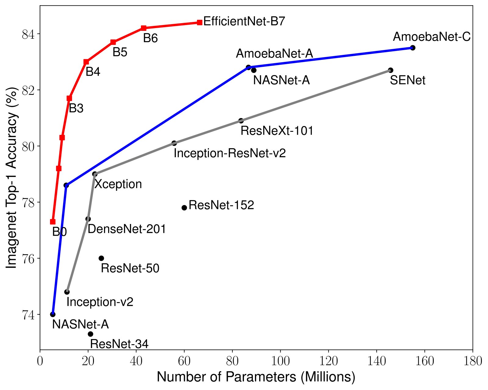
Figure 1 and Figure 5 illustrates the parameters-accuracy and FLOPS-accuracy curve for representative ConvNets, where our scaled EfficientNet models achieve better accuracy with much fewer parameters and FLOPS than other ConvNets. Notably, our EfficientNet models are not only small, but also computational cheaper. For example, our EfficientNet-B3 achieves higher accuracy than ResNeXt-101 (Xie et al., 2017) using 18x fewer FLOPS.
图1和图 没有显示具有代表性的ConvNet的参数精确度和FLOPS精确度曲线,我们经扩大的高效Net模型比其他ConvNet的参数和FLOPS更准确。 值得注意的是,我们的高效网络模型不仅规模小,而且计算成本低廉。 例如,我们的效率网-B3的精度高于ResNEXt-101(Xie等人,2017年)使用18x减少FLOPS.
To validate the latency, we have also measured the inference latency for a few representative CovNets on a real CPU as shown in Table 4, where we report average latency over 20 runs. Our EfficientNet-B1 runs 5.7x faster than the widely used ResNet-152, while EfficientNet-B7 runs about 6.1x faster than GPipe (Huang et al., 2018), suggesting our EfficientNets are indeed fast on real hardware.
为了证实这种暂时性,我们还测量了几个有代表性的CovNets在真正的CPU上的推断延迟性,如表4所示,我们报告的平均延迟超过20次。 我们的高效网-B1运行5.7x比广泛使用的ResNet-152运行快,而高效网-B7运行**6.1x则比GPipe运行快(Huang等人,2018年),说明我们的高效网在真正的硬件上确实快.
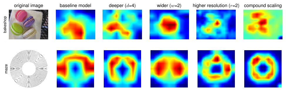
Figure 7: Class Activation Map (CAM) (Zhou et al., 2016) for Models with different scaling methods- Our compound scaling method allows the scaled model (last column) to focus on more relevant regions with more object details. Model details are in Table 7.
图7:具有不同缩放方法的模型的分类激活图(CAM)(Zhou等人,2016年) 我们的复合缩放方法使得缩放模型(最后一列)能够专注于更多对象细节的更相关区域. 模式细节见表7。
5.3 Transfer Learning Results for EfficientNet
5.3 EfficientNet 的迁移学习结果
| Dataset | Train Size | Test Size | #Classes |
|---|---|---|---|
| CIFAR-10 (Krizhevsky & Hinton, 2009) | 50,000 | 10,000 | 10 |
| CIFAR-100 (Krizhevsky & Hinton, 2009) | 50,000 | 10,000 | 100 |
| Birdsnap (Berg et al., 2014) | 47,386 | 2,443 | 500 |
| Stanford Cars (Krause et al., 2013) | 8,144 | 8,041 | 196 |
| Flowers (Nilsback & Zisserman, 2008) | 2,040 | 6,149 | 102 |
| FGVC Aircraft (Maji et al., 2013) | 6,667 | 3,333 | 100 |
| Oxford-IIIT Pets (Parkhi et al., 2012) | 3,680 | 3,369 | 37 |
| Food-101 (Bossard et al., 2014) | 75,750 | 25,250 | 101 |
Table 6: Transfer Learning Datasets.
| 数据集 | 列车大小 | 测试大小 | # 分类 # |
|---|---|---|---|
| CIFAR-10(Kettazhevsky & Hinton,2009年) | 50,000 | 10,000 | 10 |
| CIFAR-100(Krizhevsky & Hinton,2009年) | 50,000 | 10,000 | 100 |
| Birdsnap(Berg等人,2014年) | 47,386 | 2,443 | 500 |
| 斯坦福汽车(Krause等人,2013年) | 8,144 | 8,041 | 196 |
| 花(Nilsback & Zisserman,2008年). | 2,040 | 6,149 | 102 |
| FGVC飞机(Maji等人,2013年) | 6,667 | 3,333 | 100 |
| Oxford-IIIT Pets(Parkhi等人,2012年) | 3,680 | 3,369 | 37 |
| Food-101(Bossard等人,2014年) | 75,750 | 25,250 | 101 |
表6:** 转让学习数据集**。
We have also evaluated our EfficientNet on a list of commonly used transfer learning datasets, as shown in Table 6. We borrow the same training settings from (Kornblith et al., 2019) and (Huang et al., 2018), which take ImageNet pretrained checkpoints and finetune on new datasets.
如表6所示,我们还根据常用的转移学习数据集清单评估了我们的高效网络。 我们从(Kornblith等人,2019年)和(Huang等人,2018年)借用同样的训练环境,这些训练环境占用了ImageNet预先训练的检查站,并对新的数据集进行了微调。
Table 5 shows the transfer learning performance: (1) Compared to public available models, such as NASNet-A (Zoph et al., 2018) and Inception-v4 (Szegedy et al., 2017), our EfficientNet models achieve better accuracy with 4.7x average (up to 21x) parameter reduction. (2) Compared to state-of-the-art models, including DAT (Ngiam et al., 2018) that dynamically synthesizes training data and GPipe (Huang et al., 2018) that is trained with specialized pipeline parallelism, our EfficientNet models still surpass their accuracy in 5 out of 8 datasets, but using 9.6x fewer parameters
表5列示了转移学习性能: (1)与公有模式相比,如NASNet-A(Zoph等人,2018年)和Inception-v4(Szegedy等人,2017年),我们高效的Net模型以4.7x平均(最多21x)参数还原实现更好的精度. (2) 与先进模型相比,包括动态综合训练数据的DAT(Ngiam等人,2018年)和经过专门管道平行化训练的GPipe(Huang等人,2018年),我们的高效网络模型在8个数据集中有5个仍然超过其精确度,但使用9.6x更少的参数
Figure 6 compares the accuracy-parameters curve for a variety of models. In general, our EfficientNets consistently achieve better accuracy with an order of magnitude fewer parameters than existing models, including ResNet (He et al., 2016), DenseNet (Huang et al., 2017), Inception (Szegedy et al., 2017), and NASNet (Zoph et al., 2018).
图6比较了各种模型的精度参数曲线. 总体而言,我们的高效网络的精确度持续提高,其参数数量比现有模型少,包括ResNet(He等人,2016年)、DenseNet(Huang等人,2017年)、Inception(Szegedy等人,2017年)和NASNet(Zoph等人,2018年)。
6 Discussion
6 讨论
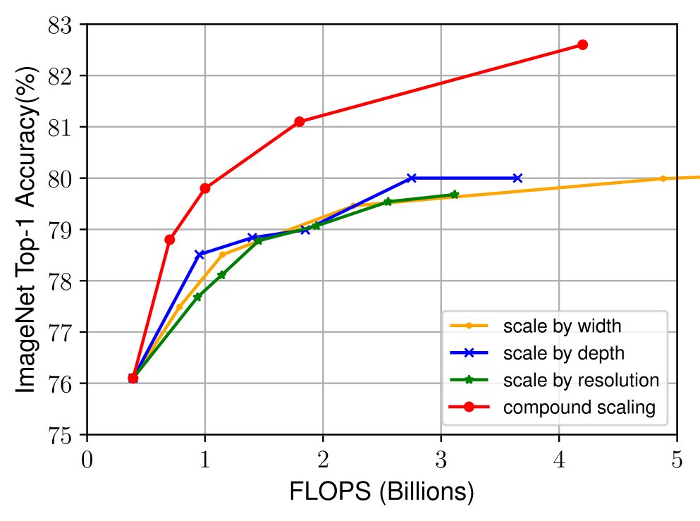
Figure 8: Scaling Up EfficientNet-B0 with Different Methods.
图 事实上,在2000年12月31日终了的2002-2003两年期中,有7个P-4和2个P-3员额的空缺。
| Model | FLOPS | Top-1 Acc. |
|---|---|---|
| Baseline model (EfficientNet-B0) | 0.4B | 77.3% |
| Scale model by depth (=4) | 1.8B | 79.0% |
| Scale model by width (=2) | 1.8B | 78.9% |
| Scale model by resolution (=2) | 1.9B | 79.1% |
| Compound Scale (=1.4, =1.2, =1.3) | 1.8B | 81.1% |
Table 7: Scaled Models Used in Figure 7.
| 型号 | FLOPS | 顶级1Acc. |
|---|---|---|
| 基线模型(EfficientNet-B0) | 0.4B (韩语) | 77.3% |
| 按深度划分的尺度模型(=4) | 1.8B (韩语) | 79.0% |
| 按宽度划分的缩放模型(=2) | 1.8B (韩语) | 78.9% |
| 按分辨率划分的比例模型(=2) | 1.9B (韩语) | 79.1% |
| ** 比额表(=1.4,=1.2,=1.3)** | 页:1 | 81.1% |
表7:** 图7使用的规模模型**
To disentangle the contribution of our proposed scaling method from the EfficientNet architecture, Figure 8 compares the ImageNet performance of different scaling methods for the same EfficientNet-B0 baseline network. In general, all scaling methods improve accuracy with the cost of more FLOPS, but our compound scaling method can further improve accuracy, by up to 2.5%, than other single-dimension scaling methods, suggesting the importance of our proposed compound scaling.
为了将我们提议的缩放方法与 " 高效网络 " 结构区分开来,图8比较了同一 " 高效网络-B0 " 基线网络不同缩放方法的图像网络性能。 一般来说,所有的缩放方法都会随着更多FLOPS的成本而提高精度,但我们的复合缩放方法可以比其他单位缩放方法进一步提高精度,最高可达2.5%,这表明我们提议的化合物缩放的重要性.
In order to further understand why our compound scaling method is better than others, Figure 7 compares the class activation map (Zhou et al., 2016) for a few representative models with different scaling methods. All these models are scaled from the same baseline, and their statistics are shown in Table 7. Images are randomly picked from ImageNet validation set. As shown in the figure, the model with compound scaling tends to focus on more relevant regions with more object details, while other models are either lack of object details or unable to capture all objects in the images.
为了进一步理解为什么我们的化合物缩放方法比其他方法更好,图7将分类激活图(Zhou et al.,2016)比较为少数具有代表性的模型,采用不同的缩放方法. 所有这些模型都从同一基线中按比例调整,其统计数据见表7。 从ImageNet验证集中随机选择图像. 如图所示,具有复合缩放的模型倾向于以更多对象细节的更相关区域为重点,而其他模型要么缺乏对象细节,要么无法捕捉图像中的所有对象.
7 Conclusion
7 结论
In this paper, we systematically study ConvNet scaling and identify that carefully balancing network width, depth, and resolution is an important but missing piece, preventing us from better accuracy and efficiency. To address this issue, we propose a simple and highly effective compound scaling method, which enables us to easily scale up a baseline ConvNet to any target resource constraints in a more principled way, while maintaining model efficiency. Powered by this compound scaling method, we demonstrate that a mobile-size EfficientNet model can be scaled up very effectively, surpassing state-of-the-art accuracy with an order of magnitude fewer parameters and FLOPS, on both ImageNet and five commonly used transfer learning datasets.
在本文中,我们系统地研究ConvNet的缩放,并确定仔细平衡网络宽度、深度和分辨率是一个重要的但缺失的作品,使我们无法提高准确度和效率。 为了解决这一问题,我们提出了一种简单和高效的复合规模化方法,使我们能够以更具原则性的方式将基线ConvNet扩大至任何目标资源限制,同时保持模式效率。 在这种复合缩放方法的推动下,我们表明,移动大小的高效网络模型可以非常有效地升级,在ImageNet和五个常用的传输学习数据集上,其精确度超过了最先进的参数和FLOPS。
Acknowledgements
致谢
We thank Ruoming Pang, Vijay Vasudevan, Alok Aggarwal, Barret Zoph, Hongkun Yu, Jonathon Shlens, Raphael Gontijo Lopes, Yifeng Lu, Daiyi Peng, Xiaodan Song, Samy Bengio, Jeff Dean, and the Google Brain team for their help.
感谢鲁明庞,维杰·瓦苏德万,阿洛克·阿加瓦尔,巴雷特·佐夫,洪昆羽,约纳顿·斯伦斯,拉斐尔·贡蒂霍·洛佩斯,吕义丰,戴义鹏,小丹松,萨米·本乔,杰夫·迪恩,以及谷歌脑团队的帮助.
Appendix
附录
Since 2017, most research papers only report and compare ImageNet validation accuracy; this paper also follows this convention for better comparison. In addition, we have also verified the test accuracy by submitting our predictions on the 100k test set images to http://image-net.org; results are in Table 8. As expected, the test accuracy is very close to the validation accuracy.
自2017年起,大多数研究论文只报告和比较ImageNet验证准确性;本文也遵循这个惯例进行更好的比较. 此外,我们还通过向http://image-net.org提交对100k测试集图像的预测,核实了测试准确性;结果见表8。 如预期,测试精度与验证精度非常接近.
| B0 | B1 | B2 | B3 | B4 | B5 | B6 | B7 | |
|---|---|---|---|---|---|---|---|---|
| Val top1 | 77.11 | 79.13 | 80.07 | 81.59 | 82.89 | 83.60 | 83.95 | 84.26 |
| Test top1 | 77.23 | 79.17 | 80.16 | 81.72 | 82.94 | 83.69 | 84.04 | 84.33 |
| Val top5 | 93.35 | 94.47 | 94.90 | 95.67 | 96.37 | 96.71 | 96.76 | 96.97 |
| Test top5 | 93.45 | 94.43 | 94.98 | 95.70 | 96.27 | 96.64 | 96.86 | 96.94 |
Table 8: ImageNet Validation vs. Test Top-1/5 Accuracy.
| 我还以为是B0 | B1级 | B2级 | B3级 | B4级 | B5级 | B6级 | B7级 | |
|---|---|---|---|---|---|---|---|---|
| 瓦尔顶部1 | 77.11 | 79.13 | 80.07 | 81.59 | 82.89 | 83.60 | 83.95 | 84.26 |
| 测试顶端1 | 77.23 | 79.17 | 80.16 | 81.72 | 82.94 | 83.69 | 84.04 | 84.33 |
| 瓦尔顶端5 | 93.35 | 94.47 | 94.90 | 95.67 | 96.37 | 96.71 | 96.76 | 96.97 |
| 测试顶端5 | 93.45 | 94.43 | 94.98 | 95.70 | 96.27 | 96.64 | 96.86 | 96.94 |
表8:ImageNet验证与Test Top-1/5精确度。
References
参考文献
Berg et al. (2014) Berg, T., Liu, J., Woo Lee, S., Alexander, M. L., Jacobs, D. W., and Belhumeur, P. N. Birdsnap: Large-scale fine-grained visual categorization of birds. CVPR , pp. 2011–2018, 2014.
Bossard et al. (2014) Bossard, L., Guillaumin, M., and Van Gool, L. Food-101–mining discriminative components with random forests. ECCV , pp. 446–461, 2014.
Cai et al. (2019) Cai, H., Zhu, L., and Han, S. Proxylessnas: Direct neural architecture search on target task and hardware. ICLR , 2019.
Chollet (2017) Chollet, F. Xception: Deep learning with depthwise separable convolutions. CVPR , pp. 1610–02357, 2017.
Cubuk et al. (2019) Cubuk, E. D., Zoph, B., Mane, D., Vasudevan, V., and Le, Q. V. Autoaugment: Learning augmentation policies from data. CVPR , 2019.
Elfwing et al. (2018) Elfwing, S., Uchibe, E., and Doya, K. Sigmoid-weighted linear units for neural network function approximation in reinforcement learning. Neural Networks , 107:3–11, 2018.
Gholami et al. (2018) Gholami, A., Kwon, K., Wu, B., Tai, Z., Yue, X., Jin, P., Zhao, S., and Keutzer, K. Squeezenext: Hardware-aware neural network design. ECV Workshop at CVPR’18 , 2018.
Han et al. (2016) Han, S., Mao, H., and Dally, W. J. Deep compression: Compressing deep neural networks with pruning, trained quantization and huffman coding. ICLR , 2016.
He et al. (2016) He, K., Zhang, X., Ren, S., and Sun, J. Deep residual learning for image recognition. CVPR , pp. 770–778, 2016.
He et al. (2017) He, K., Gkioxari, G., Dollár, P., and Girshick, R. Mask r-cnn. ICCV , pp. 2980–2988, 2017.
He et al. (2018) He, Y., Lin, J., Liu, Z., Wang, H., Li, L.-J., and Han, S. Amc: Automl for model compression and acceleration on mobile devices. ECCV , 2018.
Hendrycks & Gimpel (2016) Hendrycks, D. and Gimpel, K. Gaussian error linear units (gelus). arXiv preprint arXiv:1606.08415 , 2016.
Howard et al. (2017) Howard, A. G., Zhu, M., Chen, B., Kalenichenko, D., Wang, W., Weyand, T., Andreetto, M., and Adam, H. Mobilenets: Efficient convolutional neural networks for mobile vision applications. arXiv preprint arXiv:1704.04861 , 2017.
Hu et al. (2018) Hu, J., Shen, L., and Sun, G. Squeeze-and-excitation networks. CVPR , 2018.
Huang et al. (2016) Huang, G., Sun, Y., Liu, Z., Sedra, D., and Weinberger, K. Q. Deep networks with stochastic depth. ECCV , pp. 646–661, 2016.
Huang et al. (2017) Huang, G., Liu, Z., Van Der Maaten, L., and Weinberger, K. Q. Densely connected convolutional networks. CVPR , 2017.
Huang et al. (2018) Huang, Y., Cheng, Y., Chen, D., Lee, H., Ngiam, J., Le, Q. V., and Chen, Z. Gpipe: Efficient training of giant neural networks using pipeline parallelism. arXiv preprint arXiv:1808.07233 , 2018.
Iandola et al. (2016) Iandola, F. N., Han, S., Moskewicz, M. W., Ashraf, K., Dally, W. J., and Keutzer, K. Squeezenet: Alexnet-level accuracy with 50x fewer parameters and < < 0.5 mb model size. arXiv preprint arXiv:1602.07360 , 2016.
Ioffe & Szegedy (2015) Ioffe, S. and Szegedy, C. Batch normalization: Accelerating deep network training by reducing internal covariate shift. ICML , pp. 448–456, 2015.
Kornblith et al. (2019) Kornblith, S., Shlens, J., and Le, Q. V. Do better imagenet models transfer better? CVPR , 2019.
Krause et al. (2013) Krause, J., Deng, J., Stark, M., and Fei-Fei, L. Collecting a large-scale dataset of fine-grained cars. Second Workshop on Fine-Grained Visual Categorizatio , 2013.
Krizhevsky & Hinton (2009) Krizhevsky, A. and Hinton, G. Learning multiple layers of features from tiny images. Technical Report , 2009.
Krizhevsky et al. (2012) Krizhevsky, A., Sutskever, I., and Hinton, G. E. Imagenet classification with deep convolutional neural networks. In NIPS , pp. 1097–1105, 2012.
Lin & Jegelka (2018) Lin, H. and Jegelka, S. Resnet with one-neuron hidden layers is a universal approximator. NeurIPS , pp. 6172–6181, 2018.
Lin et al. (2017) Lin, T.-Y., Dollár, P., Girshick, R., He, K., Hariharan, B., and Belongie, S. Feature pyramid networks for object detection. CVPR , 2017.
Liu et al. (2018) Liu, C., Zoph, B., Shlens, J., Hua, W., Li, L.-J., Fei-Fei, L., Yuille, A., Huang, J., and Murphy, K. Progressive neural architecture search. ECCV , 2018.
Lu et al. (2018) Lu, Z., Pu, H., Wang, F., Hu, Z., and Wang, L. The expressive power of neural networks: A view from the width. NeurIPS , 2018.
Ma et al. (2018) Ma, N., Zhang, X., Zheng, H.-T., and Sun, J. Shufflenet v2: Practical guidelines for efficient cnn architecture design. ECCV , 2018.
Mahajan et al. (2018) Mahajan, D., Girshick, R., Ramanathan, V., He, K., Paluri, M., Li, Y., Bharambe, A., and van der Maaten, L. Exploring the limits of weakly supervised pretraining. arXiv preprint arXiv:1805.00932 , 2018.
Maji et al. (2013) Maji, S., Rahtu, E., Kannala, J., Blaschko, M., and Vedaldi, A. Fine-grained visual classification of aircraft. arXiv preprint arXiv:1306.5151 , 2013.
Ngiam et al. (2018) Ngiam, J., Peng, D., Vasudevan, V., Kornblith, S., Le, Q. V., and Pang, R. Domain adaptive transfer learning with specialist models. arXiv preprint arXiv:1811.07056 , 2018.
Nilsback & Zisserman (2008) Nilsback, M.-E. and Zisserman, A. Automated flower classification over a large number of classes. ICVGIP , pp. 722–729, 2008.
Parkhi et al. (2012) Parkhi, O. M., Vedaldi, A., Zisserman, A., and Jawahar, C. Cats and dogs. CVPR , pp. 3498–3505, 2012.
Raghu et al. (2017) Raghu, M., Poole, B., Kleinberg, J., Ganguli, S., and Sohl-Dickstein, J. On the expressive power of deep neural networks. ICML , 2017.
Ramachandran et al. (2018) Ramachandran, P., Zoph, B., and Le, Q. V. Searching for activation functions. arXiv preprint arXiv:1710.05941 , 2018.
Real et al. (2019) Real, E., Aggarwal, A., Huang, Y., and Le, Q. V. Regularized evolution for image classifier architecture search. AAAI , 2019.
Russakovsky et al. (2015) Russakovsky, O., Deng, J., Su, H., Krause, J., Satheesh, S., Ma, S., Huang, Z., Karpathy, A., Khosla, A., Bernstein, M., et al. Imagenet large scale visual recognition challenge. International Journal of Computer Vision , 115(3):211–252, 2015.
Sandler et al. (2018) Sandler, M., Howard, A., Zhu, M., Zhmoginov, A., and Chen, L.-C. Mobilenetv2: Inverted residuals and linear bottlenecks. CVPR , 2018.
Sharir & Shashua (2018) Sharir, O. and Shashua, A. On the expressive power of overlapping architectures of deep learning. ICLR , 2018.
Srivastava et al. (2014) Srivastava, N., Hinton, G., Krizhevsky, A., Sutskever, I., and Salakhutdinov, R. Dropout: a simple way to prevent neural networks from overfitting. The Journal of Machine Learning Research , 15(1):1929–1958, 2014.
Szegedy et al. (2015) Szegedy, C., Liu, W., Jia, Y., Sermanet, P., Reed, S., Anguelov, D., Erhan, D., Vanhoucke, V., and Rabinovich, A. Going deeper with convolutions. CVPR , pp. 1–9, 2015.
Szegedy et al. (2016) Szegedy, C., Vanhoucke, V., Ioffe, S., Shlens, J., and Wojna, Z. Rethinking the inception architecture for computer vision. CVPR , pp. 2818–2826, 2016.
Szegedy et al. (2017) Szegedy, C., Ioffe, S., Vanhoucke, V., and Alemi, A. A. Inception-v4, inception-resnet and the impact of residual connections on learning. AAAI , 4:12, 2017.
Tan et al. (2019) Tan, M., Chen, B., Pang, R., Vasudevan, V., Sandler, M., Howard, A., and Le, Q. V. MnasNet: Platform-aware neural architecture search for mobile. CVPR , 2019.
Xie et al. (2017) Xie, S., Girshick, R., Dollár, P., Tu, Z., and He, K. Aggregated residual transformations for deep neural networks. CVPR , pp. 5987–5995, 2017.
Yang et al. (2018) Yang, T.-J., Howard, A., Chen, B., Zhang, X., Go, A., Sze, V., and Adam, H. Netadapt: Platform-aware neural network adaptation for mobile applications. ECCV , 2018.
Zagoruyko & Komodakis (2016) Zagoruyko, S. and Komodakis, N. Wide residual networks. BMVC , 2016.
Zhang et al. (2017) Zhang, X., Li, Z., Loy, C. C., and Lin, D. Polynet: A pursuit of structural diversity in very deep networks. CVPR , pp. 3900–3908, 2017.
Zhang et al. (2018) Zhang, X., Zhou, X., Lin, M., and Sun, J. Shufflenet: An extremely efficient convolutional neural network for mobile devices. CVPR , 2018.
Zhou et al. (2016) Zhou, B., Khosla, A., Lapedriza, A., Oliva, A., and Torralba, A. Learning deep features for discriminative localization. CVPR , pp. 2921–2929, 2016.
Zoph & Le (2017) Zoph, B. and Le, Q. V. Neural architecture search with reinforcement learning. ICLR , 2017.
Zoph et al. (2018) Zoph, B., Vasudevan, V., Shlens, J., and Le, Q. V. Learning transferable architectures for scalable image recognition. CVPR , 2018.