EfficientDet: Scalable and Efficient Object Detection

EfficientDet：可扩展且高效的目标检测

Mingxing Tan Ruoming Pang Quoc V. Le Google Research, Brain Team { tanmingxing, rpang, qvl}@google.com

Abstract

摘要

Model efficiency has become increasingly important in computer vision. In this paper, we systematically study neural network architecture design choices for object detection and propose several key optimizations to improve efficiency. First, we propose a weighted bi-directional feature pyramid network (BiFPN), which allows easy and fast multi-scale feature fusion; Second, we propose a compound scaling method that uniformly scales the resolution, depth, and width for all backbone, feature network, and box/class prediction networks at the same time. Based on these optimizations and better backbones, we have developed a new family of object detectors, called EfficientDet, which consistently achieve much better efficiency than prior art across a wide spectrum of resource constraints. In particular, with single-model and single-scale, our EfficientDet-D7 achieves state-of-the-art 55.1 AP on COCO test-dev with 77M parameters and 410B FLOPs[^1], being 4x – 9x smaller and using 13x – 42x fewer FLOPs than previous detectors. Code is available at https://github.com/google/automl/tree/master/efficientdet.

模型效率在计算机视觉中变得越来越重要。本文系统地研究目标检测的神经网络结构设计，并提出若干提高效率的关键改进。首先，我们提出加权双向特征金字塔网络（BiFPN），使多尺度特征融合更简便、也更快；其次，我们提出一种复合缩放方法，同时对骨干网络、特征网络以及边框/类别预测网络的分辨率、深度和宽度做统一缩放。基于这些改进和更优的骨干网络，我们得到一族新的目标检测器，称为 EfficientDet，在很宽的资源约束范围内，效率都稳定优于已有方法。具体而言，在单模型、单尺度设置下，我们的 EfficientDet-D7 在 COCO test-dev 上达到当时最高的 55.1 AP，参数量为 7700 万，FLOPs 为 410B[^1]，体积比先前检测器小 4 倍到 9 倍，FLOPs 少 13 倍到 42 倍。代码见 https://github.com/google/automl/tree/master/efficientdet。

[^1]: Similar to [14, 39], FLOPs denotes number of multiply-adds.

[^1]：与 [14, 39] 类似，FLOPs 表示乘加次数。

1 Introduction

1 引言

Tremendous progresses have been made in recent years towards more accurate object detection; meanwhile, state-of-the-art object detectors also become increasingly more expensive. For example, the latest AmoebaNet-based NAS-FPN detector [45] requires 167M parameters and 3045B FLOPs (30x more than RetinaNet [24]) to achieve state-of-the-art accuracy. The large model sizes and expensive computation costs deter their deployment in many real-world applications such as robotics and self-driving cars where model size and latency are highly constrained. Given these real-world resource constraints, model efficiency becomes increasingly important for object detection.

近年来，目标检测的精度取得了巨大进展；与此同时，最先进的检测器也变得越来越昂贵。例如，最新的基于 AmoebaNet 的 NAS-FPN 检测器 [45] 需要 1.67 亿参数和 3045B FLOPs（约为 RetinaNet [24] 的 30 倍）才能达到当时最高精度。模型体积大、计算代价高，限制了它们在机器人和自动驾驶等对模型大小和延迟要求很严的实际场景中的部署。面对这些现实的资源约束，模型效率对目标检测变得越来越重要。

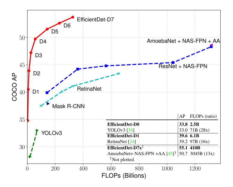
Figure 1: Model FLOPs vs. COCO accuracy – All numbers are for single-model single-scale. Our EfficientDet achieves new state-of-the-art 55.1% COCO AP with much fewer parameters and FLOPs than previous detectors. More studies on different backbones and FPN/NAS-FPN/BiFPN are in Table 4 and 5. Complete results are in Table 2.

图 1：模型 FLOPs 与 COCO 精度 – 所有数字均为单模型、单尺度。我们的 EfficientDet 在参数量和 FLOPs 远少于先前检测器的情况下，达到新的最高水平 55.1% COCO AP。关于不同骨干网络以及 FPN/NAS-FPN/BiFPN 的更多实验见 Table 4 和 Table 5。完整结果见 Table 2。

There have been many previous works aiming to develop more efficient detector architectures, such as one-stage [27, 33, 34, 24] and anchor-free detectors [21, 44, 40], or compress existing models [28, 29]. Although these methods tend to achieve better efficiency, they usually sacrifice accuracy. Moreover, most previous works only focus on a specific or a small range of resource requirements, but the variety of real-world applications, from mobile devices to datacenters, often demand different resource constraints.

已有不少工作试图设计更高效的检测器结构，例如单阶段检测器 [27, 33, 34, 24] 和无锚框检测器 [21, 44, 40]，或压缩已有模型 [28, 29]。这些方法往往能提高效率，却通常要牺牲精度。此外，大多数已有工作只关注某一段或很窄的资源需求，而真实应用从移动设备到数据中心，往往面对不同的资源约束。

A natural question is: Is it possible to build a scalable detection architecture with both higher accuracy and better efficiency across a wide spectrum of resource constraints (e.g., from 3B to 300B FLOPs)? This paper aims to tackle this problem by systematically studying various design choices of detector architectures. Based on the one-stage detector paradigm, we examine the design choices for backbone, feature fusion, and class/box network, and identify two main challenges:

一个自然的问题是：能否构建一种可缩放的检测结构，在很宽的资源约束范围（例如，从 3B 到 300B FLOPs）内，同时具有更高精度和更好效率？本文希望通过系统研究检测器结构的各种设计选择来回答这个问题。我们以单阶段检测器为出发点，考察骨干网络、特征融合和类别/边框网络的设计，并找出两个主要难点：

Challenge 1: efficient multi-scale feature fusion – Since introduced in [23], FPN has been widely used for multi-scale feature fusion. Recently, PANet [26], NAS-FPN [10], and other studies [20, 18, 42] have developed more network structures for cross-scale feature fusion. While fusing different input features, most previous works simply sum them up without distinction; however, since these different input features are at different resolutions, we observe they usually contribute to the fused output feature unequally. To address this issue, we propose a simple yet highly effective weighted bi-directional feature pyramid network (BiFPN), which introduces learnable weights to learn the importance of different input features, while repeatedly applying top-down and bottom-up multi-scale feature fusion.

难点 1：高效的多尺度特征融合 – 自 [23] 提出以来，FPN 已被广泛用于多尺度特征融合。近来，PANet [26]、NAS-FPN [10] 以及其他研究 [20, 18, 42] 为跨尺度特征融合设计了更多网络结构。在融合不同输入特征时，已有工作大多直接把它们相加、不加区分；然而这些输入特征分辨率不同，我们观察到它们对融合后输出特征的贡献通常并不相等。为此，我们提出一种简单而有效的加权双向特征金字塔网络（BiFPN）：引入可学习权重来学习不同输入特征的重要性，并反复进行自上而下和自下而上的多尺度特征融合。

Challenge 2: model scaling – While previous works mainly rely on bigger backbone networks [24, 35, 34, 10] or larger input image sizes [13, 45] for higher accuracy, we observe that scaling up feature network and box/class prediction network is also critical when taking into account both accuracy and efficiency. Inspired by recent works [39], we propose a compound scaling method for object detectors, which jointly scales up the resolution/depth/width for all backbone, feature network, box/class prediction network.

难点 2：模型缩放 – 已有工作为了提高精度，主要依赖更大的骨干网络 [24, 35, 34, 10] 或更大的输入图像 [13, 45]；我们则观察到，在同时考虑精度和效率时，放大特征网络和边框/类别预测网络同样关键。受近期工作 [39] 启发，我们为检测器提出一种复合缩放方法，同时放大骨干网络、特征网络和边框/类别预测网络的分辨率、深度与宽度。

Finally, we also observe that the recently introduced EfficientNets [39] achieve better efficiency than previous commonly used backbones. Combining EfficientNet backbones with our propose BiFPN and compound scaling, we have developed a new family of object detectors, named EfficientDet, which consistently achieve better accuracy with much fewer parameters and FLOPs than previous object detectors. Figure 1 and Figure 4 show the performance comparison on COCO dataset [25]. Under similar accuracy constraint, our EfficientDet uses 28x fewer FLOPs than YOLOv3 [34], 30x fewer FLOPs than RetinaNet [24], and 19x fewer FLOPs than the recent ResNet based NAS-FPN [10]. In particular, with single-model and single test-time scale, our EfficientDet-D7 achieves state-of-the-art 55.1 AP with 77M parameters and 410B FLOPs, outperforming previous best detector [45] by 4 AP while being 2.7x smaller and using 7.4x fewer FLOPs. Our EfficientDet is also up to 4x to 11x faster on GPU/CPU than previous detectors.

最后，我们还观察到，最近提出的 EfficientNets [39] 比此前常用的骨干网络效率更高。把 EfficientNet 骨干与我们提出的 BiFPN 和复合缩放结合起来，我们得到一族新的目标检测器，称为 EfficientDet，在参数量和 FLOPs 明显更少的情况下，精度稳定优于已有检测器。图 1 和图 4 给出了在 COCO 数据集 [25] 上的性能对比。在相近精度约束下，我们的 EfficientDet 所用 FLOPs 比 YOLOv3 [34] 少 28 倍，比 RetinaNet [24] 少 30 倍，比近期基于 ResNet 的 NAS-FPN [10] 少 19 倍。特别地，在单模型和单测试尺度下，我们的 EfficientDet-D7 以 7700 万参数和 410B FLOPs 达到当时最高的 55.1 AP，比此前最好的检测器 [45] 高 4 个 AP，体积小 2.7 倍，FLOPs 少 7.4 倍。在 GPU/CPU 上，我们的 EfficientDet 也最多可比先前检测器快 4 倍到 11 倍。

With simple modifications, we also demonstrate that our single-model single-scale EfficientDet achieves 81.74% mIOU accuracy with 18B FLOPs on Pascal VOC 2012 semantic segmentation, outperforming DeepLabV3+ [6] by 1.7% better accuracy with 9.8x fewer FLOPs.

稍作修改后，我们还表明，单模型、单尺度的 EfficientDet 在 Pascal VOC 2012 语义分割上以 18B FLOPs 达到 81.74% 的 mIOU，精度比 DeepLabV3+ [6] 高 1.7 个百分点，FLOPs 少 9.8 倍。

2 Related Work

2 相关工作

One-Stage Detectors:

Existing object detectors are mostly categorized by whether they have a region-of-interest proposal step (two-stage [11, 35, 5, 13]) or not (one-stage [36, 27, 33, 24]). While two-stage detectors tend to be more flexible and more accurate, one-stage detectors are often considered to be simpler and more efficient by leveraging predefined anchors [17]. Recently, one-stage detectors have attracted substantial attention due to their efficiency and simplicity [21, 42, 44]. In this paper, we mainly follow the one-stage detector design, and we show it is possible to achieve both better efficiency and higher accuracy with optimized network architectures.

单阶段检测器：

已有的目标检测器大多按是否包含兴趣区域提议步骤来划分：有这一步的是两阶段方法 [11, 35, 5, 13]，没有的是单阶段方法 [36, 27, 33, 24]。两阶段检测器往往更灵活、也更准，单阶段检测器则通常被认为更简单、更高效，因为它借助预定义的锚框 [17]。近来，单阶段检测器因其效率和简洁而受到大量关注 [21, 42, 44]。本文主要沿用单阶段检测器的设计，并表明通过优化网络结构，可以同时获得更好的效率和更高的精度。

Multi-Scale Feature Representations: One of the main difficulties in object detection is to effectively represent and process multi-scale features. Earlier detectors often directly perform predictions based on the pyramidal feature hierarchy extracted from backbone networks [4, 27, 36]. As one of the pioneering works, feature pyramid network (FPN) [23] proposes a top-down pathway to combine multi-scale features. Following this idea, PANet [26] adds an extra bottom-up path aggregation network on top of FPN; STDL [43] proposes a scale-transfer module to exploit cross-scale features; M2det [42] proposes a U-shape module to fuse multi-scale features, and G-FRNet [2] introduces gate units for controlling information flow across features. More recently, NAS-FPN [10] leverages neural architecture search to automatically design feature network topology. Although it achieves better performance, NAS-FPN requires thousands of GPU hours during search, and the resulting feature network is irregular and thus difficult to interpret. In this paper, we aim to optimize multi-scale feature fusion with a more intuitive and principled way.

多尺度特征表示： 目标检测的一个主要困难，是有效地表示并处理多尺度特征。较早的检测器往往直接在骨干网络提取的金字塔特征层次上做预测 [4, 27, 36]。作为开创性工作之一，特征金字塔网络（FPN）[23] 提出用一条自上而下的通路来组合多尺度特征。沿着这一思路，PANet [26] 在 FPN 之上增加一条自下而上的路径聚合网络；STDL [43] 提出尺度迁移模块来利用跨尺度特征；M2det [42] 提出 U 形模块融合多尺度特征；G-FRNet [2] 则引入门控单元来控制特征之间的信息流动。更近一些，NAS-FPN [10] 借助神经架构搜索自动设计特征网络拓扑。它虽然效果更好，但搜索需要数千 GPU 小时，得到的特征网络也不规则，因而难以解释。本文希望用更直观、也更有原则的方式，来优化多尺度特征融合。

Model Scaling: In order to obtain better accuracy, it is common to scale up a baseline detector by employing bigger backbone networks (e.g., from mobile-size models [38, 16] and ResNet [14], to ResNeXt [41] and AmoebaNet [32]), or increasing input image size (e.g., from 512x512 [24] to 1536x1536 [45]). Some recent works [10, 45] show that increasing the channel size and repeating feature networks can also lead to higher accuracy. These scaling methods mostly focus on single or limited scaling dimensions. Recently, [39] demonstrates remarkable model efficiency for image classification by jointly scaling up network width, depth, and resolution. Our proposed compound scaling method for object detection is mostly inspired by [39].

模型缩放： 为了获得更高精度，常见做法是放大一个基线检测器：换更大的骨干网络（例如，从移动端规模的模型 [38, 16] 和 ResNet [14]，到 ResNeXt [41] 和 AmoebaNet [32]），或增大输入图像尺寸（例如，从 512×512 [24] 到 1536×1536 [45]）。近期一些工作 [10, 45] 还表明，增加通道数并重复堆叠特征网络也能提高精度。这些缩放方法大多只关注单一或有限的几个维度。最近，[39] 通过同时放大网络宽度、深度和分辨率，在图像分类上展现出很高的模型效率。我们为检测提出的复合缩放方法，主要受到 [39] 的启发。

3 BiFPN

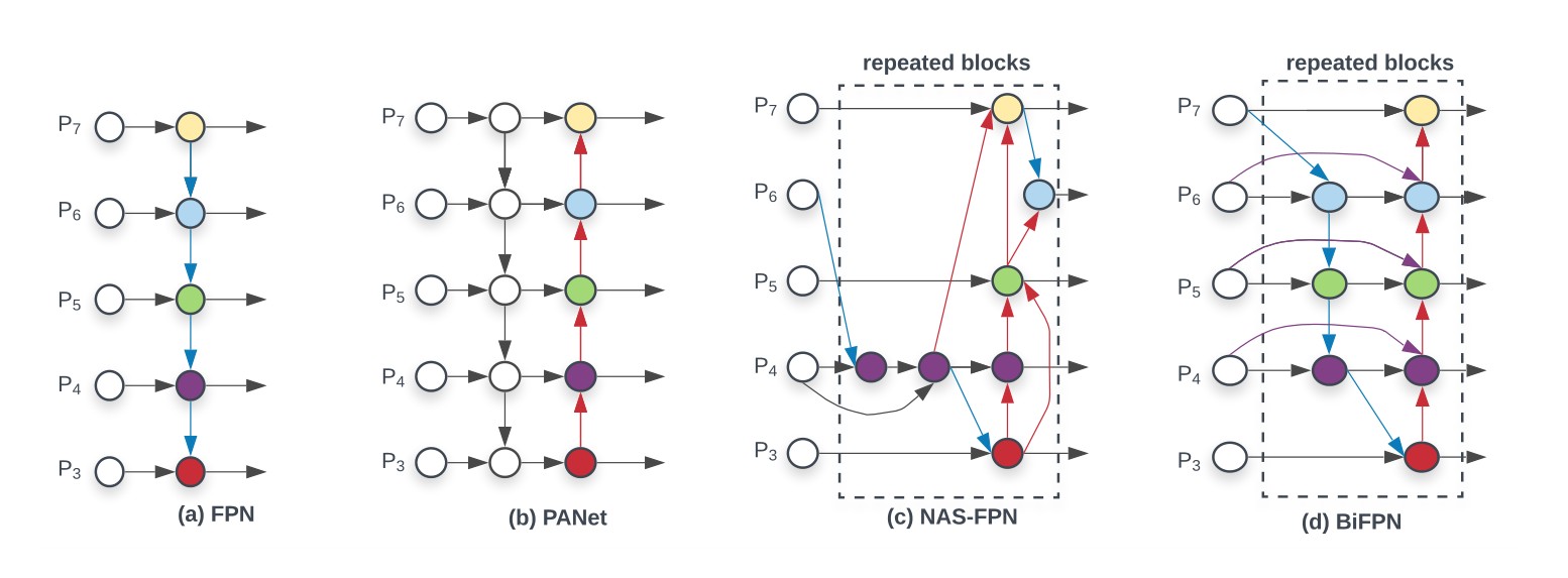
Figure 2: Feature network design – (a) FPN [23] introduces a top-down pathway to fuse multi-scale features from level 3 to 7 ($P_{3}$ - $P_{7}$); (b) PANet [26] adds an additional bottom-up pathway on top of FPN; (c) NAS-FPN [10] use neural architecture search to find an irregular feature network topology and then repeatedly apply the same block; (d) is our BiFPN with better accuracy and efficiency trade-offs.

图 2：特征网络设计 – (a) FPN [23] 引入一条自上而下的通路，融合第 3 到第 7 层的多尺度特征（$P_{3}$–$P_{7}$）；(b) PANet [26] 在 FPN 之上再加一条自下而上的通路；(c) NAS-FPN [10] 用神经架构搜索得到不规则的特征网络拓扑，再反复套用同一模块；(d) 是我们的 BiFPN，在精度和效率之间有更好的折中。

In this section, we first formulate the multi-scale feature fusion problem, and then introduce the main ideas for our proposed BiFPN: efficient bidirectional cross-scale connections and weighted feature fusion.

本节先把多尺度特征融合问题形式化，再介绍我们所提 BiFPN 的主要想法：高效的双向跨尺度连接，以及加权特征融合。

3.1 Problem Formulation

3.1 问题形式化

Multi-scale feature fusion aims to aggregate features at different resolutions. Formally, given a list of multi-scale features $\vec{P}^{in}=(P^{in}_{l_{1}},P^{in}_{l_{2}},...)$, where $P^{in}_{l_{i}}$ represents the feature at level $l_{i}$, our goal is to find a transformation $f$ that can effectively aggregate different features and output a list of new features: $\vec{P}^{out}=f(\vec{P}^{in})$. As a concrete example, Figure 2(a) shows the conventional top-down FPN [23]. It takes level 3-7 input features $\vec{P}^{in}=(P^{in}_{3},...P^{in}_{7})$, where $P^{in}_{i}$ represents a feature level with resolution of $1/2^{i}$ of the input images. For instance, if input resolution is 640x640, then $P^{in}_{3}$ represents feature level 3 ($640/2^{3}=80$) with resolution 80x80, while $P^{in}_{7}$ represents feature level 7 with resolution 5x5. The conventional FPN aggregates multi-scale features in a top-down manner:

多尺度特征融合的目标，是把不同分辨率的特征聚合起来。形式上，给定一组多尺度特征 $\vec{P}^{in}=(P^{in}_{l_{1}},P^{in}_{l_{2}},...)$，其中 $P^{in}_{l_{i}}$ 表示第 $l_{i}$ 层的特征，我们希望找到一个变换 $f$，能够有效地聚合这些特征，并输出一组新特征：$\vec{P}^{out}=f(\vec{P}^{in})$。作为一个具体例子，图 2(a) 给出了常规的自上而下 FPN [23]。它接收第 3 到第 7 层的输入特征 $\vec{P}^{in}=(P^{in}_{3},...P^{in}_{7})$，其中 $P^{in}_{i}$ 表示分辨率为输入图像 $1/2^{i}$ 的特征层。例如，若输入分辨率是 640×640，则 $P^{in}_{3}$ 表示第 3 层特征（$640/2^{3}=80$），分辨率为 80×80，而 $P^{in}_{7}$ 表示第 7 层特征，分辨率为 5×5。常规 FPN 按自上而下的方式聚合多尺度特征：

$$\displaystyle P^{out}_{7} \\ \displaystyle=Conv(P^{in}_{7}) \\ \displaystyle P^{out}_{6} \\ \displaystyle=Conv(P^{in}_{6}+Resize(P^{out}_{7})) \\ \displaystyle... \\ \displaystyle P^{out}_{3} \\ \displaystyle=Conv(P^{in}_{3}+Resize(P^{out}_{4}))$$

where $Resize$ is usually a upsampling or downsampling op for resolution matching, and $Conv$ is usually a convolutional op for feature processing.

其中 $Resize$ 通常是用于匹配分辨率的上采样或下采样操作，$Conv$ 通常是用于特征处理的卷积。

3.2 Cross-Scale Connections

3.2 跨尺度连接

Conventional top-down FPN is inherently limited by the one-way information flow. To address this issue, PANet [26] adds an extra bottom-up path aggregation network, as shown in Figure 2(b). Cross-scale connections are further studied in [20, 18, 42]. Recently, NAS-FPN [10] employs neural architecture search to search for better cross-scale feature network topology, but it requires thousands of GPU hours during search and the found network is irregular and difficult to interpret or modify, as shown in Figure 2(c).

常规的自上而下 FPN 受限于单向信息流。为解决这一问题，PANet [26] 增加了一条额外的自下而上路径聚合网络，如图 2(b) 所示。跨尺度连接在 [20, 18, 42] 中得到了进一步研究。近来，NAS-FPN [10] 用神经架构搜索寻找更好的跨尺度特征网络拓扑，但搜索需要数千 GPU 小时，得到的网络不规则，既难以解释也难以修改，如图 2(c) 所示。

By studying the performance and efficiency of these three networks (Table 5), we observe that PANet achieves better accuracy than FPN and NAS-FPN, but with the cost of more parameters and computations. To improve model efficiency, this paper proposes several optimizations for cross-scale connections: First, we remove those nodes that only have one input edge. Our intuition is simple: if a node has only one input edge with no feature fusion, then it will have less contribution to feature network that aims at fusing different features. This leads to a simplified bi-directional network; Second, we add an extra edge from the original input to output node if they are at the same level, in order to fuse more features without adding much cost; Third, unlike PANet [26] that only has one top-down and one bottom-up path, we treat each bidirectional (top-down & bottom-up) path as one feature network layer, and repeat the same layer multiple times to enable more high-level feature fusion. Section 4.2 will discuss how to determine the number of layers for different resource constraints using a compound scaling method. With these optimizations, we name the new feature network as bidirectional feature pyramid network (BiFPN), as shown in Figure 2 and 3.

通过比较这三种网络的精度和效率（表 5），我们观察到 PANet 的精度高于 FPN 和 NAS-FPN，但代价是更多的参数和计算量。为提高模型效率，本文对跨尺度连接做了几处优化：第一，删掉只有一条输入边的节点。直觉很简单：如果一个节点只有一条输入边、并不做特征融合，那么它对以融合不同特征为目标的特征网络贡献就较小。这样可以得到一个简化的双向网络；第二，如果原始输入和输出节点位于同一层，就再加一条从输入到输出的边，以便在不增加太多代价的情况下融合更多特征；第三，与只有一条自上而下通路和一条自下而上通路的 PANet [26] 不同，我们把每一条双向（自上而下与自下而上）通路当作一个特征网络层，并把同一层重复多次，以便做更多高层特征融合。第 4.2 节会讨论如何用复合缩放方法，按不同资源约束决定层数。经过这些优化，我们把新的特征网络称为双向特征金字塔网络（BiFPN），如图 2 和图 3 所示。

3.3 Weighted Feature Fusion

3.3 加权特征融合

When fusing features with different resolutions, a common way is to first resize them to the same resolution and then sum them up. Pyramid attention network [22] introduces global self-attention upsampling to recover pixel localization, which is further studied in [10]. All previous methods treat all input features equally without distinction. However, we observe that since different input features are at different resolutions, they usually contribute to the output feature unequally. To address this issue, we propose to add an additional weight for each input, and let the network to learn the importance of each input feature. Based on this idea, we consider three weighted fusion approaches:

在融合不同分辨率的特征时，常见做法是先把它们缩放到同一分辨率，再直接相加。金字塔注意力网络 [22] 引入全局自注意力上采样来恢复像素定位，这一做法在 [10] 中得到了进一步研究。已有方法都把各路输入特征同等看待、不加区分。然而我们观察到，由于不同输入特征分辨率不同，它们对输出特征的贡献通常并不相等。为解决这一问题，我们建议为每路输入增加一个额外权重，让网络学习各路输入特征的重要性。基于这一想法，我们考虑三种加权融合方式：

Unbounded fusion: $O=\sum_{i}w_{i}\cdot I_{i}$, where $w_{i}$ is a learnable weight that can be a scalar (per-feature), a vector (per-channel), or a multi-dimensional tensor (per-pixel). We find a scale can achieve comparable accuracy to other approaches with minimal computational costs. However, since the scalar weight is unbounded, it could potentially cause training instability. Therefore, we resort to weight normalization to bound the value range of each weight.

无界融合： $O=\sum_{i}w_{i}\cdot I_{i}$，其中 $w_{i}$ 是可学习权重，可以是标量（按特征）、向量（按通道）或多维张量（按像素）。我们发现，用一个标量缩放就能在计算代价很小的情况下，达到与其他方式相近的精度。不过，由于标量权重没有上界，有可能造成训练不稳定。因此，我们转而用权重归一化来限制每个权重的取值范围。

Softmax-based fusion: $O=\sum_{i}\cfrac{e^{w_{i}}}{\sum_{j}e^{w_{j}}}\cdot I_{i}$. An intuitive idea is to apply softmax to each weight, such that all weights are normalized to be a probability with value range from 0 to 1, representing the importance of each input. However, as shown in our ablation study in section 6.3, the extra softmax leads to significant slowdown on GPU hardware. To minimize the extra latency cost, we further propose a fast fusion approach.

基于 softmax 的融合： $O=\sum_{i}\cfrac{e^{w_{i}}}{\sum_{j}e^{w_{j}}}\cdot I_{i}$。一个直观的想法是对每个权重做 softmax，使所有权重被归一化成 0 到 1 之间的概率，用来表示各路输入的重要性。然而，如第 6.3 节的消融所示，额外的 softmax 会在 GPU 上带来明显的减速。为尽量降低这份额外延迟，我们进一步提出一种快速融合方法。

Fast normalized fusion: $O=\sum_{i}\cfrac{w_{i}}{\epsilon+\sum_{j}w_{j}}\cdot I_{i}$, where $w_{i}\geq 0$ is ensured by applying a Relu after each $w_{i}$, and $\epsilon=0.0001$ is a small value to avoid numerical instability. Similarly, the value of each normalized weight also falls between 0 and 1, but since there is no softmax operation here, it is much more efficient. Our ablation study shows this fast fusion approach has very similar learning behavior and accuracy as the softmax-based fusion, but runs up to 30% faster on GPUs (Table 6).

快速归一化融合： $O=\sum_{i}\cfrac{w_{i}}{\epsilon+\sum_{j}w_{j}}\cdot I_{i}$，其中通过对每个 $w_{i}$ 后接 ReLU 来保证 $w_{i}\geq 0$，$\epsilon=0.0001$ 是为避免数值不稳定而设的小量。与前一种方式类似，每个归一化权重的取值也落在 0 到 1 之间，但这里没有 softmax 运算，因而效率高得多。消融实验表明，这种快速融合与基于 softmax 的融合在学习行为和精度上非常接近，但在 GPU 上最多可快约 30%（表 6）。

Our final BiFPN integrates both the bidirectional cross-scale connections and the fast normalized fusion. As a concrete example, here we describe the two fused features at level 6 for BiFPN shown in Figure 2(d):

最终的 BiFPN 同时采用了双向跨尺度连接和快速归一化融合。作为一个具体例子，这里给出图 2(d) 中 BiFPN 在第 6 层的两路融合特征：

$$\displaystyle P^{td}_{6} \\ \displaystyle=Conv\left(\frac{w_{1}\cdot P^{in}_{6}+w_{2}\cdot Resize(P^{in}_{7})}{w_{1}+w_{2}+\epsilon}\right) \\ \displaystyle P^{out}_{6} \\ \displaystyle=Conv\left(\frac{w^{\prime}_{1}\cdot P^{in}_{6}+w^{\prime}_{2}\cdot P^{td}_{6}+w^{\prime}_{3}\cdot Resize(P^{out}_{5})}{w^{\prime}_{1}+w^{\prime}_{2}+w^{\prime}_{3}+\epsilon}\right)$$

where $P^{td}_{6}$ is the intermediate feature at level 6 on the top-down pathway, and $P^{out}_{6}$ is the output feature at level 6 on the bottom-up pathway. All other features are constructed in a similar manner. Notably, to further improve the efficiency, we use depthwise separable convolution [7, 37] for feature fusion, and add batch normalization and activation after each convolution.

其中 $P^{td}_{6}$ 是自上而下通路上第 6 层的中间特征，$P^{out}_{6}$ 是自下而上通路上第 6 层的输出特征。其余特征用类似方式构造。值得注意的是，为进一步提高效率，我们在特征融合中使用深度可分离卷积 [7, 37]，并在每次卷积后加入批归一化和激活函数。

4 EfficientDet

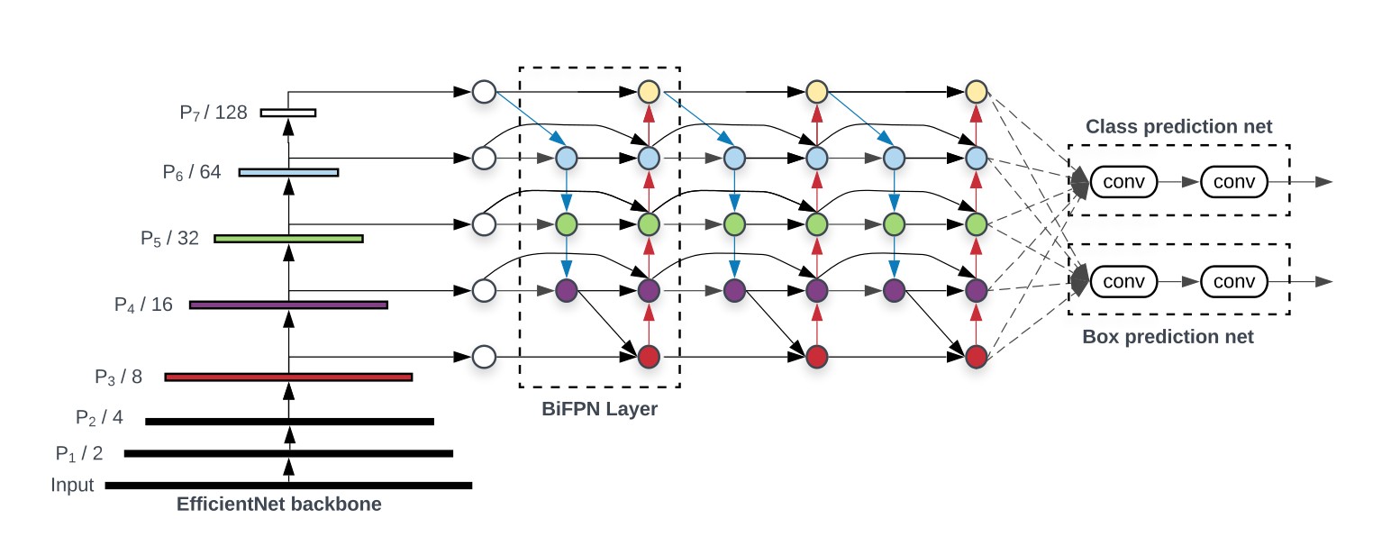
Figure 3: EfficientDet architecture – It employs EfficientNet [39] as the backbone network, BiFPN as the feature network, and shared class/box prediction network. Both BiFPN layers and class/box net layers are repeated multiple times based on different resource constraints as shown in Table 1.

图 3：EfficientDet 结构 – 以 EfficientNet [39] 为骨干网络，BiFPN 为特征网络，并使用共享的类别/边框预测网络。BiFPN 层和类别/边框网络层会按不同资源约束重复多次，具体配置见表 1。

Based on our BiFPN, we have developed a new family of detection models named EfficientDet. In this section, we will discuss the network architecture and a new compound scaling method for EfficientDet.

基于 BiFPN，我们设计了一族新的检测模型，称为 EfficientDet。本节将讨论其网络结构，以及一种新的复合缩放方法。

4.1 EfficientDet Architecture

4.1 EfficientDet 结构

Figure 3 shows the overall architecture of EfficientDet, which largely follows the one-stage detectors paradigm [27, 33, 23, 24]. We employ ImageNet-pretrained EfficientNets as the backbone network. Our proposed BiFPN serves as the feature network, which takes level 3-7 features {$P_{3},P_{4},P_{5},P_{6},P_{7}$} from the backbone network and repeatedly applies top-down and bottom-up bidirectional feature fusion. These fused features are fed to a class and box network to produce object class and bounding box predictions respectively. Similar to [24], the class and box network weights are shared across all levels of features.

图 3 给出了 EfficientDet 的整体结构，它大体沿用单阶段检测器的范式 [27, 33, 23, 24]。我们以在 ImageNet 上预训练的 EfficientNets 作为骨干网络。所提出的 BiFPN 充当特征网络，从骨干网络取出第 3 到第 7 层特征 $\{P_{3},P_{4},P_{5},P_{6},P_{7}\}$，并反复进行自上而下与自下而上的双向特征融合。这些融合后的特征再分别送入类别网络和边框网络，产生物体类别和边界框预测。与 [24] 类似，类别网络和边框网络的权重在所有特征层之间共享。

4.2 Compound Scaling

4.2 复合缩放

Aiming at optimizing both accuracy and efficiency, we would like to develop a family of models that can meet a wide spectrum of resource constraints. A key challenge here is how to scale up a baseline EfficientDet model.

为了同时优化精度和效率，我们希望得到一族能够覆盖很宽资源约束范围的模型。这里的一个关键问题是：如何放大一个基线 EfficientDet 模型。

Previous works mostly scale up a baseline detector by employing bigger backbone networks (e.g., ResNeXt [41] or AmoebaNet [32]), using larger input images, or stacking more FPN layers [10]. These methods are usually ineffective since they only focus on a single or limited scaling dimensions. Recent work [39] shows remarkable performance on image classification by jointly scaling up all dimensions of network width, depth, and input resolution. Inspired by these works [10, 39], we propose a new compound scaling method for object detection, which uses a simple compound coefficient $\phi$ to jointly scale up all dimensions of backbone , BiFPN, class/box network, and resolution. Unlike [39], object detectors have much more scaling dimensions than image classification models, so grid search for all dimensions is prohibitive expensive. Therefore, we use a heuristic-based scaling approach, but still follow the main idea of jointly scaling up all dimensions.

已有工作放大基线检测器时，大多是换更大的骨干网络（例如 ResNeXt [41] 或 AmoebaNet [32]）、使用更大的输入图像，或堆叠更多 FPN 层 [10]。这些方法往往效果有限，因为它们只关注单一或很少几个缩放维度。近期工作 [39] 表明，同时放大网络宽度、深度和输入分辨率，可以在图像分类上取得很好的效果。受这些工作 [10, 39] 启发，我们为检测提出一种新的复合缩放方法：用一个简单的复合系数 $\phi$，同时放大骨干网络、BiFPN、类别/边框网络以及分辨率的各个维度。与 [39] 不同，检测器的缩放维度比图像分类模型多得多，对所有维度做网格搜索代价过高。因此我们采用启发式的缩放方式，但仍然遵循同时放大所有维度这一主要想法。

Backbone network –

we reuse the same width/depth scaling coefficients of EfficientNet-B0 to B6 [39] such that we can easily reuse their ImageNet-pretrained checkpoints.

骨干网络 –

我们沿用 EfficientNet-B0 到 B6 [39] 的宽度/深度缩放系数，以便直接复用它们在 ImageNet 上预训练的检查点。

BiFPN network –

we linearly increase BiFPN depth $D_{bifpn}$ (#layers) since depth needs to be rounded to small integers. For BiFPN width $W_{bifpn}$ (#channels), exponentially grow BiFPN width $W_{bifpn}$ (#channels) as similar to [39]. Specifically, we perform a grid search on a list of values {1.2, 1.25, 1.3, 1.35, 1.4, 1.45}, and pick the best value 1.35 as the BiFPN width scaling factor. Formally, BiFPN width and depth are scaled with the following equation:

BiFPN 网络 –

由于深度需要取整为较小的整数，我们让 BiFPN 的深度 $D_{bifpn}$（层数）线性增加。对于 BiFPN 的宽度 $W_{bifpn}$（通道数），则与 [39] 类似地做指数增长。具体而言，我们在 $\{1.2, 1.25, 1.3, 1.35, 1.4, 1.45\}$ 这一组数值上做网格搜索，并选定效果最好的 1.35 作为 BiFPN 宽度缩放因子。形式上，BiFPN 的宽度和深度按下列公式缩放：

$$W_{bifpn}=64\cdot\left(1.35^{\phi}\right),\quad\quad D_{bifpn}=3+\phi \tag{1}$$

Box/class prediction network –

we fix their width to be always the same as BiFPN (i.e., $W_{pred}=W_{bifpn}$), but linearly increase the depth (#layers) using equation:

边框/类别预测网络 –

我们把它们的宽度固定为始终与 BiFPN 相同（即 $W_{pred}=W_{bifpn}$），但按下列公式线性增加深度（层数）：

$$D_{box}=D_{class}=3+\lfloor\phi/3\rfloor \tag{2}$$

Input image resolution –

Since feature level 3-7 are used in BiFPN, the input resolution must be dividable by $2^{7}=128$, so we linearly increase resolutions using equation:

输入图像分辨率 –

由于 BiFPN 使用第 3 到第 7 层特征，输入分辨率必须能被 $2^{7}=128$ 整除，因此我们按下列公式线性增大分辨率：

$$R_{input}=512+\phi\cdot 128 \tag{3}$$

Following Equations 1,2,3 with different $\phi$, we have developed EfficientDet-D0 ($\phi=0$) to D7 ($\phi=7$) as shown in Table 1, where D7 and D7x have the same BiFPN and head, but D7 uses higher resolution and D7x uses larger backbone network and one more feature level (from $P_{3}$ to $P_{8}$). Notably, our compound scaling is heuristic-based and might not be optimal, but we will show that this simple scaling method can significantly improve efficiency than other single-dimension scaling methods in Figure 6.

按公式 1、2、3 取不同的 $\phi$，我们得到如表 1 所示的 EfficientDet-D0（$\phi=0$）到 D7（$\phi=7$）。其中 D7 和 D7x 使用相同的 BiFPN 和预测头，但 D7 使用更高分辨率，D7x 则使用更大的骨干网络，并多一层特征（从 $P_{3}$ 到 $P_{8}$）。需要说明的是，我们的复合缩放是启发式的，不一定最优，但我们会在图 6 中表明，这种简单的缩放方法比其他单维度缩放能明显提高效率。

	Input size	Backbone Network	BiFPN #channels	BiFPN #layers	Box/class #layers
	$R_{input}$		$W_{bifpn}$	$D_{bifpn}$	$D_{class}$
D0 ($\phi=0$)	512	B0	64	3	3
D1 ($\phi=1$)	640	B1	88	4	3
D2 ($\phi=2$)	768	B2	112	5	3
D3 ($\phi=3$)	896	B3	160	6	4
D4 ($\phi=4$)	1024	B4	224	7	4
D5 ($\phi=5$)	1280	B5	288	7	4
D6 ($\phi=6$)	1280	B6	384	8	5
D7 ($\phi=7$)	1536	B6	384	8	5
D7x	1536	B7	384	8	5

Table 1: Scaling configs for EfficientDet D0-D6 – $\phi$ is the compound coefficient that controls all other scaling dimensions; BiFPN, box/class net, and input size are scaled up using equation 1, 2, 3 respectively.

	输入尺寸	骨干网络	BiFPN 通道数	BiFPN 层数	边框/类别头层数
	$R_{input}$		$W_{bifpn}$	$D_{bifpn}$	$D_{class}$
D0 ($\phi=0$)	512	B0	64	3	3
D1 ($\phi=1$)	640	B1	88	4	3
D2 ($\phi=2$)	768	B2	112	5	3
D3 ($\phi=3$)	896	B3	160	6	4
D4 ($\phi=4$)	1024	B4	224	7	4
D5 ($\phi=5$)	1280	B5	288	7	4
D6 ($\phi=6$)	1280	B6	384	8	5
D7 ($\phi=7$)	1536	B6	384	8	5
D7x	1536	B7	384	8	5

表 1：EfficientDet D0–D6 的缩放配置 – $\phi$ 是控制其余缩放维度的复合系数；BiFPN、边框/类别网络和输入尺寸 分别按公式 1、2、3 放大。

Model	test-dev $AP$	test-dev $AP_{50}$	test-dev $AP_{75}$	val $AP$	Params	Ratio	FLOPs	Ratio	TitianV	V100
EfficientDet-D0 (512)	34.6	53.0	37.1	34.3	3.9M	1x	2.5B	1x	12	10.2
YOLOv3 [34]	33.0	57.9	34.4	-	-	-	71B	28x	-	-
EfficientDet-D1 (640)	40.5	59.1	43.7	40.2	6.6M	1x	6.1B	1x	16	13.5
RetinaNet-R50 (640) [24]	39.2	58.0	42.3	39.2	34M	6.7x	97B	16x	25	-
RetinaNet-R101 (640)[24]	39.9	58.5	43.0	39.8	53M	8.0x	127B	21x	32	-
EfficientDet-D2 (768)	43.9	62.7	47.6	43.5	8.1M	1x	11B	1x	23	17.7
Detectron2 Mask R-CNN R101-FPN [1]	-	-	-	42.9	63M	7.7x	164B	15x	-	56‡
Detectron2 Mask R-CNN X101-FPN [1]	-	-	-	44.3	107M	13x	277B	25x	-	103‡
EfficientDet-D3 (896)	47.2	65.9	51.2	46.8	12M	1x	25B	1x	37	29.0
ResNet-50 + NAS-FPN (1024) [10]	44.2	-	-	-	60M	5.1x	360B	15x	64	-
ResNet-50 + NAS-FPN (1280) [10]	44.8	-	-	-	60M	5.1x	563B	23x	99	-
ResNet-50 + NAS-FPN (1280@384)[10]	45.4	-	-	-	104M	8.7x	1043B	42x	150	-
EfficientDet-D4 (1024)	49.7	68.4	53.9	49.3	21M	1x	55B	1x	65	42.8
AmoebaNet+ NAS-FPN +AA(1280)[45]	-	-	-	48.6	185M	8.8x	1317B	24x	246	-
EfficientDet-D5 (1280)	51.5	70.5	56.1	51.3	34M	1x	135B	1x	128	72.5
Detectron2 Mask R-CNN X152 [1]	-	-	-	50.2	-	-	-	-	-	234‡
EfficientDet-D6 (1280)	52.6	71.5	57.2	52.2	52M	1x	226B	1x	169	92.8
AmoebaNet+ NAS-FPN +AA(1536)[45]	-	-	-	50.7	209M	4.0x	3045B	13x	489	-
EfficientDet-D7 (1536)	53.7	72.4	58.4	53.4	52M		325B		232	122
EfficientDet-D7x (1536)	55.1	74.3	59.9	54.4	77M		410B		285	153

We omit ensemble and test-time multi-scale results [30, 12]. RetinaNet APs are reproduced with our trainer and others are from papers.

‡Latency numbers with ‡ are from detectron2, and others are measured on the same machine (TensorFlow2.1 + CUDA10.1, no TensorRT).

Table 2: EfficientDet performance on COCO [25] – Results are for single-model single-scale. test-dev is the COCO test set and val is the validation set. Params and FLOPs denote the number of parameters and multiply-adds. Latency is for inference with batch size 1. AA denotes auto-augmentation [45]. We group models together if they have similar accuracy, and compare their model size, FLOPs, and latency in each group.

模型	test-dev $AP$	test-dev $AP_{50}$	test-dev $AP_{75}$	val $AP$	参数量	倍率	FLOPs	倍率	TitianV	V100
EfficientDet-D0 (512)	34.6	53.0	37.1	34.3	3.9M	1x	2.5B	1x	12	10.2
YOLOv3 [34]	33.0	57.9	34.4	-	-	-	71B	28x	-	-
EfficientDet-D1 (640)	40.5	59.1	43.7	40.2	6.6M	1x	6.1B	1x	16	13.5
RetinaNet-R50 (640) [24]	39.2	58.0	42.3	39.2	34M	6.7x	97B	16x	25	-
RetinaNet-R101 (640)[24]	39.9	58.5	43.0	39.8	53M	8.0x	127B	21x	32	-
EfficientDet-D2 (768)	43.9	62.7	47.6	43.5	8.1M	1x	11B	1x	23	17.7
Detectron2 Mask R-CNN R101-FPN [1]	-	-	-	42.9	63M	7.7x	164B	15x	-	56‡
Detectron2 Mask R-CNN X101-FPN [1]	-	-	-	44.3	107M	13x	277B	25x	-	103‡
EfficientDet-D3 (896)	47.2	65.9	51.2	46.8	12M	1x	25B	1x	37	29.0
ResNet-50 + NAS-FPN (1024) [10]	44.2	-	-	-	60M	5.1x	360B	15x	64	-
ResNet-50 + NAS-FPN (1280) [10]	44.8	-	-	-	60M	5.1x	563B	23x	99	-
ResNet-50 + NAS-FPN (1280@384)[10]	45.4	-	-	-	104M	8.7x	1043B	42x	150	-
EfficientDet-D4 (1024)	49.7	68.4	53.9	49.3	21M	1x	55B	1x	65	42.8
AmoebaNet+ NAS-FPN +AA(1280)[45]	-	-	-	48.6	185M	8.8x	1317B	24x	246	-
EfficientDet-D5 (1280)	51.5	70.5	56.1	51.3	34M	1x	135B	1x	128	72.5
Detectron2 Mask R-CNN X152 [1]	-	-	-	50.2	-	-	-	-	-	234‡
EfficientDet-D6 (1280)	52.6	71.5	57.2	52.2	52M	1x	226B	1x	169	92.8
AmoebaNet+ NAS-FPN +AA(1536)[45]	-	-	-	50.7	209M	4.0x	3045B	13x	489	-
EfficientDet-D7 (1536)	53.7	72.4	58.4	53.4	52M		325B		232	122
EfficientDet-D7x (1536)	55.1	74.3	59.9	54.4	77M		410B		285	153

我们略去集成和测试时多尺度的结果 [30, 12]。RetinaNet 的 AP 由我们的训练程序复现，其余数字来自原论文。

标有 ‡ 的延迟数字来自 Detectron2，其余均在同一台机器上测得（TensorFlow 2.1 + CUDA 10.1，未使用 TensorRT）。

表 2：EfficientDet 在 COCO 上的表现 [25] – 结果均为单模型、单尺度。test-dev 是 COCO 测试集，val 是验证集。Params 和 FLOPs 分别表示参数量和乘加次数。延迟为 batch size 为 1 时的推理时间。AA 表示自动数据增强 [45]。我们把精度接近的模型放在同一组，比较每组内的模型大小、FLOPs 和延迟。

5 Experiments

5 实验

5.1 EfficientDet for Object Detection

5.1 用 EfficientDet 做目标检测

We evaluate EfficientDet on COCO 2017 detection datasets [25] with 118K training images. Each model is trained using SGD optimizer with momentum 0.9 and weight decay 4e-5. Learning rate is linearly increased from 0 to 0.16 in the first training epoch and then annealed down using cosine decay rule. Synchronized batch norm is added after every convolution with batch norm decay 0.99 and epsilon 1e-3. Same as the [39], we use SiLU (Swish-1) activation [8, 15, 31] and exponential moving average with decay 0.9998. We also employ commonly-used focal loss [24] with $\alpha=0.25$ and $\gamma=1.5$, and aspect ratio {1/2, 1, 2}. During training, we apply horizontal flipping and scale jittering [0.1, 2.0], which randomly rsizes images between 0.1x and 2.0x of the original size before cropping. We apply soft-NMS [3] for eval. For D0-D6, each model is trained for 300 epochs with total batch size 128 on 32 TPUv3 cores, but to push the envelope, we train D7/D7x for 600 epochs on 128 TPUv3 cores.

我们在 COCO 2017 检测数据集 [25] 上评估 EfficientDet，训练集有 11.8 万张图像。每个模型用 SGD 优化器训练，动量为 0.9，权重衰减为 4e-5。学习率在第一个训练轮次中从 0 线性升到 0.16，随后按余弦衰减下降。每个卷积后加入同步批归一化，衰减为 0.99，epsilon 为 1e-3。与 [39] 相同，我们使用 SiLU（Swish-1）激活函数 [8, 15, 31]，以及衰减为 0.9998 的指数滑动平均。我们还采用常用的 focal loss [24]，其中 $\alpha=0.25$，$\gamma=1.5$，宽高比为 {1/2, 1, 2}。训练时使用水平翻转和尺度抖动 [0.1, 2.0]，即先把图像随机缩放到原尺寸的 0.1 倍到 2.0 倍，再裁剪。评估时使用 soft-NMS [3]。D0 到 D6 每个模型训练 300 个轮次，总 batch size 为 128，使用 32 个 TPUv3 核心；为进一步冲高结果，D7/D7x 在 128 个 TPUv3 核心上训练 600 个轮次。

Table 2 compares EfficientDet with other object detectors, under the single-model single-scale settings with no test-time augmentation. We report accuracy for both test-dev (20K test images with no public ground-truth) and val with 5K validation images. Notably, model performance depends on both network architecture and trainning settings (see appendix), but for simplicity, we only reproduce RetinaNet using our trainers and refer other models from their papers. In general, our EfficientDet achieves better efficiency than previous detectors, being 4x – 9x smaller and using 13x - 42x less FLOPs across a wide range of accuracy or resource constraints. On relatively low-accuracy regime, our EfficientDet-D0 achieves similar accuracy as YOLOv3 with 28x fewer FLOPs. Compared to RetinaNet [24] and Mask-RCNN [13], our EfficientDet achieves similar accuracy with up to 8x fewer parameters and 21x fewer FLOPs. On high-accuracy regime, our EfficientDet also consistently outperforms recent object detectors [10, 45] with much fewer parameters and FLOPs. In particular, our single-model single-scale EfficientDet-D7x achieves a new state-of-the-art 55.1 AP on test-dev, outperforming prior art by a large margin in both accuracy (+4 AP) and efficiency (7x fewer FLOPs).

表 2 在单模型、单尺度、不做测试时增强的设置下，把 EfficientDet 与其他目标检测器做了比较。我们同时报告 test-dev（2 万张没有公开标注的测试图像）和包含 5000 张图像的验证集 val 上的精度。需要指出的是，模型表现同时取决于网络结构和训练设置（见附录），但为简单起见，我们只用自己的训练程序复现 RetinaNet，其余模型数字直接引用原论文。总体来看，我们的 EfficientDet 效率优于先前检测器，体积小 4 倍到 9 倍，在很宽的精度或资源区间内 FLOPs 少 13 倍到 42 倍。在精度相对较低的区间，我们的 EfficientDet-D0 与 YOLOv3 精度相近，FLOPs 少 28 倍。与 RetinaNet [24] 和 Mask R-CNN [13] 相比，EfficientDet 在相近精度下参数最多少 8 倍，FLOPs 最多少 21 倍。在高精度区间，EfficientDet 也稳定优于近期检测器 [10, 45]，同时参数量和 FLOPs 少得多。特别地，单模型、单尺度的 EfficientDet-D7x 在 test-dev 上达到新的最高水平 55.1 AP，精度比已有最好结果高出较大幅度（+4 AP），效率也更高（FLOPs 少 7 倍）。

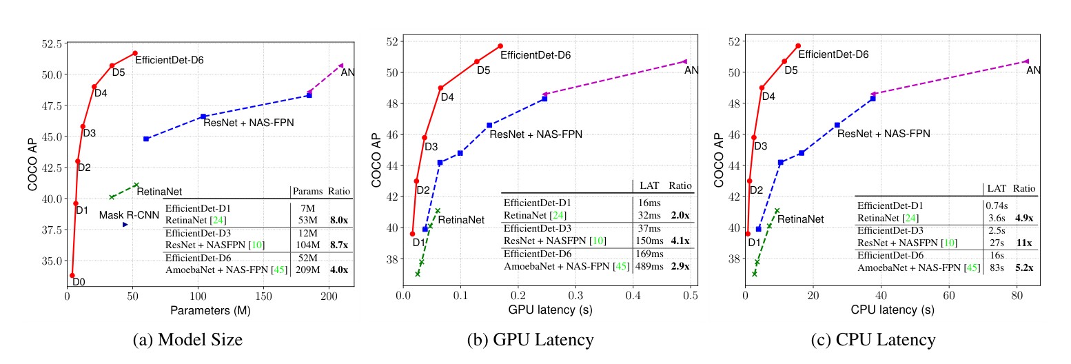
Figure 4: Model size and inference latency comparison – Latency is measured with batch size 1 on the same machine equipped with a Titan V GPU and Xeon CPU. AN denotes AmoebaNet + NAS-FPN trained with auto-augmentation [45]. Our EfficientDet models are 4x - 9x smaller, 2x - 4x faster on GPU, and 5x - 11x faster on CPU than other detectors.

图 4：模型大小与推理延迟对比 – 延迟在同一台配备 Titan V GPU 和 Xeon CPU 的机器上、以 batch size 为 1 测得。AN 表示经过自动数据增强训练的 AmoebaNet + NAS-FPN [45]。与其他检测器相比，我们的 EfficientDet 体积小 4 倍到 9 倍，在 GPU 上快 2 倍到 4 倍，在 CPU 上快 5 倍到 11 倍。

In addition, we have also compared the inference latency on Titan-V FP32 , V100 GPU FP16, and single-thread CPU. Notably, our V100 latency is end-to-end including preprocessing and NMS postprocessing. Figure 4 illustrates the comparison on model size and GPU/CPU latency. For fair comparison, these figures only include results that are measured on the same machine with the same settings. Compared to previous detectors, EfficientDet models are up to 4.1x faster on GPU and 10.8x faster on CPU, suggesting they are also efficient on real-world hardware.

此外，我们还在 Titan-V 的 FP32、V100 GPU 的 FP16 以及单线程 CPU 上比较了推理延迟。需要说明的是，我们给出的 V100 延迟是端到端的，包含预处理和 NMS 后处理。图 4 展示了模型大小以及 GPU/CPU 延迟的对比。为公平起见，这些图只收入在同一台机器、同一设置下测得的结果。与先前检测器相比，EfficientDet 在 GPU 上最快可快 4.1 倍，在 CPU 上最快可快 10.8 倍，说明它们在真实硬件上同样高效。

5.2 EfficientDet for Semantic Segmentation

5.2 用 EfficientDet 做语义分割

While our EfficientDet models are mainly designed for object detection, we are also interested in their performance on other tasks such as semantic segmentation. Following [19], we modify our EfficientDet model to keep feature level $\{P2,P3,...,P7\}$ in BiFPN, but only use $P2$ for the final per-pixel classification. For simplicity, here we only evaluate a EfficientDet-D4 based model, which uses a ImageNet pretrained EfficientNet-B4 backbone (similar size to ResNet-50). We set the channel size to 128 for BiFPN and 256 for classification head. Both BiFPN and classification head are repeated by 3 times.

EfficientDet 主要用于目标检测，但我们也关心它在语义分割等其他任务上的表现。按照 [19]，我们修改模型，使 BiFPN 保留特征层 $\{P2,P3,...,P7\}$，但最终的逐像素分类只用 $P2$。为简单起见，这里只评估一个基于 EfficientDet-D4 的模型，骨干是在 ImageNet 上预训练的 EfficientNet-B4（规模与 ResNet-50 相近）。我们把 BiFPN 的通道数设为 128，分类头的通道数设为 256。BiFPN 和分类头都重复 3 次。

Model	mIOU	Params	FLOPs
DeepLabV3+ (ResNet-101) [6]	79.35%	-	298B
DeepLabV3+ (Xception) [6]	80.02%	-	177B
Our EfficientDet†	81.74%	17M	18B
†A modified version of EfficientDet-D4.

Table 3: Performance comparison on Pascal VOC semantic segmentation.

模型	mIOU	参数量	FLOPs
DeepLabV3+ (ResNet-101) [6]	79.35%	-	298B
DeepLabV3+ (Xception) [6]	80.02%	-	177B
我们的 EfficientDet†	81.74%	17M	18B
†基于 EfficientDet-D4 的改写版本。

表 3：在 Pascal VOC 语义分割上的性能对比。

Table 3 shows the comparison between our models and previous DeepLabV3+ [6] on Pascal VOC 2012 [9]. Notably, we exclude those results with ensemble, test-time augmentation, or COCO pretraining. Under the same single-model single-scale settings, our model achieves 1.7% better accuracy with 9.8x fewer FLOPs than the prior art of DeepLabV3+ [6]. These results suggest that EfficientDet is also quite promising for semantic segmentation.

表 3 给出了我们的模型与先前 DeepLabV3+ [6] 在 Pascal VOC 2012 [9] 上的对比。需要说明的是，我们排除了使用集成、测试时增强或 COCO 预训练的结果。在同样的单模型、单尺度设置下，我们的模型精度比当时最好的 DeepLabV3+ [6] 高 1.7 个百分点，FLOPs 少 9.8 倍。这些结果表明，EfficientDet 在语义分割上也相当有潜力。

6 Ablation Study

6 消融实验

Figure 5: Softmax vs. fast normalized feature fusion – (a) - (c) shows normalized weights (i.e., importance) during training for three representative nodes; each node has two inputs (input1 & input2) and their normalized weights always sum up to 1.

图 5：softmax 融合与快速归一化特征融合 – (a)–(c) 给出三个代表性节点在训练过程中的归一化权重（即重要性）；每个节点有两路输入（input1 和 input2），它们的归一化权重始终和为 1。

In this section, we ablate various design choices for our proposed EfficientDet. For simplicity, all accuracy results here are for COCO validation set.

本节对我们提出的 EfficientDet 中的各项设计选择做消融。为简单起见，这里的精度结果都来自 COCO 验证集。

6.1 Disentangling Backbone and BiFPN

6.1 把骨干网络和 BiFPN 分开看

Since EfficientDet uses both a powerful backbone and a new BiFPN, we want to understand how much each of them contributes to the accuracy and efficiency improvements. Table 4 compares the impact of backbone and BiFPN using RetinaNet training settings. Starting from a RetinaNet detector [24] with ResNet-50 [14] backbone and top-down FPN [23], we first replace the backbone with EfficientNet-B3, which improves accuracy by about 3 AP with slightly less parameters and FLOPs. By further replacing FPN with our proposed BiFPN, we achieve additional 4 AP gain with much fewer parameters and FLOPs. These results suggest that EfficientNet backbones and BiFPN are both crucial for our final models.

EfficientDet 同时使用了较强的骨干网络和新的 BiFPN，我们希望弄清二者分别对精度和效率提升贡献了多少。表 4 在 RetinaNet 的训练设置下比较了骨干和 BiFPN 的影响。从采用 ResNet-50 [14] 骨干和自上而下 FPN [23] 的 RetinaNet 检测器 [24] 出发，我们先把骨干换成 EfficientNet-B3，精度提高约 3 个 AP，参数量和 FLOPs 还略有下降。再把 FPN 换成本文的 BiFPN，又能额外获得 4 个 AP，同时参数量和 FLOPs 明显减少。这些结果说明，EfficientNet 骨干和 BiFPN 对最终模型都至关重要。

	AP	Parameters	FLOPs
ResNet50 + FPN	37.0	34M	97B
EfficientNet-B3 + FPN	40.3	21M	75B
EfficientNet-B3 + BiFPN	44.4	12M	24B

Table 4: Disentangling backbone and BiFPN – Starting from the standard RetinaNet (ResNet50+FPN), we first replace the backbone with EfficientNet-B3, and then replace the baseline FPN with our proposed BiFPN.

	AP	参数量	FLOPs
ResNet50 + FPN	37.0	34M	97B
EfficientNet-B3 + FPN	40.3	21M	75B
EfficientNet-B3 + BiFPN	44.4	12M	24B

表 4：把骨干网络和 BiFPN 分开看 – 从标准 RetinaNet（ResNet50+FPN）出发，我们先把骨干换成 EfficientNet-B3，再把原来的 FPN 换成本文的 BiFPN。

6.2 BiFPN Cross-Scale Connections

6.2 BiFPN 的跨尺度连接

Table 5 shows the accuracy and model complexity for feature networks with different cross-scale connections listed in Figure 2. Notably, the original FPN [23] and PANet [26] only have one top-down or bottom-up flow, but for fair comparison, here we repeat each of them multiple times and replace all convs with depthwise separable convs, which is the same as BiFPN. We use the same backbone and class/box prediction network, and the same training settings for all experiments. As we can see, the conventional top-down FPN is inherently limited by the one-way information flow and thus has the lowest accuracy. While repeated FPN+PANet achieves slightly better accuracy than NAS-FPN [10], it also requires more parameters and FLOPs. Our BiFPN achieves similar accuracy as repeated FPN+PANet, but uses much less parameters and FLOPs. With the additional weighted feature fusion, our BiFPN further achieves the best accuracy with fewer parameters and FLOPs.

表 5 给出了图 2 中所列、具有不同跨尺度连接的特征网络在精度和模型复杂度上的对比。需要说明的是，原来的 FPN [23] 和 PANet [26] 分别只有自上而下或自下而上的一路信息流，但为公平比较，这里把它们各自重复多次，并把所有卷积换成深度可分离卷积，与 BiFPN 保持一致。所有实验使用相同的骨干网络、类别/边框预测网络和训练设置。可以看到，常规的自上而下 FPN 受限于单向信息流，精度最低。重复的 FPN+PANet 精度略高于 NAS-FPN [10]，但参数量和 FLOPs 也更多。我们的 BiFPN 精度与重复的 FPN+PANet 相近，但参数量和 FLOPs 少得多。再加上加权特征融合后，BiFPN 以更少的参数量和 FLOPs 取得了最高精度。

	AP	#Params ratio	#FLOPs ratio
Repeated top-down FPN	42.29	1.0x	1.0x
Repeated FPN+PANet	44.08	1.0x	1.0x
NAS-FPN	43.16	0.71x	0.72x
Fully-Connected FPN	43.06	1.24x	1.21x
BiFPN (w/o weighted)	43.94	0.88x	0.67x
BiFPN (w/ weighted)	44.39	0.88x	0.68x

Table 5: Comparison of different feature networks – Our weighted BiFPN achieves the best accuracy with fewer parameters and FLOPs.

	AP	参数量倍率	FLOPs 倍率
Repeated top-down FPN	42.29	1.0x	1.0x
Repeated FPN+PANet	44.08	1.0x	1.0x
NAS-FPN	43.16	0.71x	0.72x
Fully-Connected FPN	43.06	1.24x	1.21x
BiFPN（不加权重）	43.94	0.88x	0.67x
BiFPN（加权重）	44.39	0.88x	0.68x

表 5：不同特征网络的对比 – 带权重的 BiFPN 以更少的参数量和 FLOPs 取得最高精度。

6.3 Softmax vs Fast Normalized Fusion

6.3 Softmax 与快速归一化融合

Model	Softmax Fusion AP	Fast Fusion AP (delta)	Speedup
Model1	33.96	33.85 (-0.11)	1.28x
Model2	43.78	43.77 (-0.01)	1.26x
Model3	48.79	48.74 (-0.05)	1.31x

Table 6: Comparison of different feature fusion – Our fast fusion achieves similar accuracy as softmax-based fusion, but runs 28% - 31% faster.

模型	Softmax 融合 AP	快速融合 AP（差值）	加速比
Model1	33.96	33.85 (-0.11)	1.28x
Model2	43.78	43.77 (-0.01)	1.26x
Model3	48.79	48.74 (-0.05)	1.31x

表 6：不同特征融合方式的对比 – 快速融合的精度与基于 softmax 的融合相近，但速度快 28% 到 31%。

As discussed in Section 3.3, we propose a fast normalized feature fusion approach to get ride of the expensive softmax while retaining the benefits of normalized weights. Table 6 compares the softmax and fast normalized fusion approaches in three detectors with different model sizes. As shown in the results, our fast normalized fusion approach achieves similar accuracy as the softmax-based fusion, but runs 1.26x - 1.31x faster on GPUs.

如第 3.3 节所述，我们提出快速归一化特征融合，以去掉代价较高的 softmax，同时保留归一化权重的好处。表 6 在三个不同规模的检测器上比较了 softmax 融合与快速归一化融合。结果显示，快速归一化融合的精度与基于 softmax 的融合相近，但在 GPU 上快 1.26 倍到 1.31 倍。

In order to further understand the behavior of softmax-based and fast normalized fusion, Figure 5 illustrates the learned weights for three feature fusion nodes randomly selected from the BiFPN layers in EfficientDet-D3. Notably, the normalized weights (e.g., $e^{w_{i}}/\sum_{j}e^{w_{j}}$ for softmax-based fusion, and $w_{i}/(\epsilon+\sum_{j}w_{j})$ for fast normalized fusion) always sum up to 1 for all inputs. Interestingly, the normalized weights change rapidly during training, suggesting different features contribute to the feature fusion unequally. Despite the rapid change, our fast normalized fusion approach always shows very similar learning behavior to the softmax-based fusion for all three nodes.

为进一步理解基于 softmax 的融合和快速归一化融合的行为，图 5 给出了从 EfficientDet-D3 的 BiFPN 层中随机选出的三个特征融合节点的学习权重。需要注意的是，归一化权重（例如，基于 softmax 的融合为 $e^{w_{i}}/\sum_{j}e^{w_{j}}$，快速归一化融合为 $w_{i}/(\epsilon+\sum_{j}w_{j})$）对所有输入始终求和为 1。有意思的是，归一化权重在训练过程中变化很快，说明不同特征对融合的贡献并不相等。尽管变化很快，快速归一化融合在所有三个节点上的学习行为，始终与基于 softmax 的融合非常接近。

6.4 Compound Scaling

6.4 复合缩放

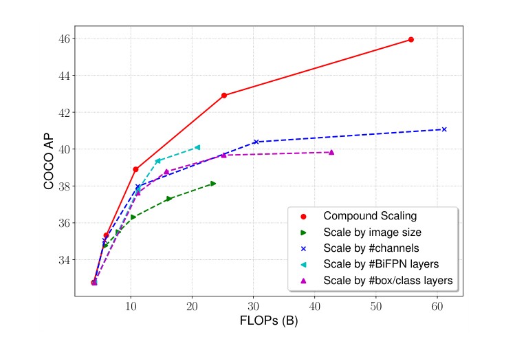
Figure 6: Comparison of different scaling methods – compound scaling achieves better accuracy and efficiency.

图 6：不同缩放方法的对比 – 复合缩放能同时取得更好的精度和效率。

As discussed in section 4.2, we employ a compound scaling method to jointly scale up all dimensions of depth/width/resolution for backbone, BiFPN, and box/class prediction networks. Figure 6 compares our compound scaling with other alternative methods that scale up a single dimension of resolution/depth/width. Although starting from the same baseline detector, our compound scaling method achieves better efficiency than other methods, suggesting the benefits of jointly scaling by better balancing difference architecture dimensions.

如第 4.2 节所述，我们采用复合缩放方法，同时放大骨干网络、BiFPN 以及边框/类别预测网络的深度、宽度和分辨率。图 6 把复合缩放与只放大分辨率、深度或宽度中单一维度的其他方法做了对比。尽管都从同一个基线检测器出发，复合缩放的效率优于其他方法，说明通过更好地平衡不同结构维度、同时进行缩放是有益的。

7 Conclusion

7 结论

In this paper, we systematically study network architecture design choices for efficient object detection, and propose a weighted bidirectional feature network and a customized compound scaling method, in order to improve accuracy and efficiency. Based on these optimizations, we develop a new family of detectors, named EfficientDet, which consistently achieve better accuracy and efficiency than the prior art across a wide spectrum of resource constraints. In particular, our scaled EfficientDet achieves state-of-the-art accuracy with much fewer parameters and FLOPs than previous object detection and semantic segmentation models.

本文系统研究了高效目标检测的网络结构设计，并提出一种加权双向特征网络，以及一种专门的复合缩放方法，以同时提高精度和效率。基于这些改进，我们得到一族新的检测器，称为 EfficientDet，在很宽的资源约束范围内，精度和效率都稳定优于已有方法。特别地，经过缩放的 EfficientDet 达到了当时最高的精度，而参数量和 FLOPs 远少于先前的目标检测和语义分割模型。

Acknowledgements

致谢

Special thanks to Golnaz Ghiasi, Adams Yu, Daiyi Peng for their help on infrastructure and discussion. We also thank Adam Kraft, Barret Zoph, Ekin D. Cubuk, Hongkun Yu, Jeff Dean, Pengchong Jin, Samy Bengio, Reed Wanderman-Milne, Tsung-Yi Lin, Xianzhi Du, Xiaodan Song, Yunxing Dai, and the Google Brain team. We thank the open source community for the contributions.

特别感谢 Golnaz Ghiasi、Adams Yu、Daiyi Peng 在基础设施和讨论上的帮助。我们也感谢 Adam Kraft、Barret Zoph、Ekin D. Cubuk、Hongkun Yu、Jeff Dean、Pengchong Jin、Samy Bengio、Reed Wanderman-Milne、Tsung-Yi Lin、Xianzhi Du、Xiaodan Song、Yunxing Dai 以及 Google Brain 团队。感谢开源社区的贡献。

References

参考文献

[1] Detectron2. https://github.com/facebookresearch/detectron2 . Accessed: 05/01/2020.

[2] Md Amirul Islam, Mrigank Rochan, Neil DB Bruce, and Yang Wang. Gated feedback refinement network for dense image labeling. CVPR , pages 3751–3759, 2017.

[3] Navaneeth Bodla, Bharat Singh, Rama Chellappa, and Larry S Davis. Soft-nms–improving object detection with one line of code. ICCV , pages 5561–5569, 2017.

[4] Zhaowei Cai, Quanfu Fan, Rogerio S Feris, and Nuno Vasconcelos. A unified multi-scale deep convolutional neural network for fast object detection. ECCV , pages 354–370, 2016.

[5] Zhaowei Cai and Nuno Vasconcelos. Cascade r-cnn: Delving into high quality object detection. CVPR , pages 6154–6162, 2018.

[6] Liang-Chieh Chen, Yukun Zhu, George Papandreou, Florian Schroff, and Hartwig Adam. Encoder-decoder with atrous separable convolution for semantic image segmentation. ECCV , 2018.

[7] François Chollet. Xception: Deep learning with depthwise separable convolutions. CVPR , pages 1610–02357, 2017.

[8] Stefan Elfwing, Eiji Uchibe, and Kenji Doya. Sigmoid-weighted linear units for neural network function approximation in reinforcement learning. Neural Networks , 107:3–11, 2018.

[9] Mark Everingham, S. M. Ali Eslami, Luc Van Gool, Christopher K. I. Williams, John Winn, and Andrew Zisserman. The pascal visual object classes challenge: A retrospective. International Journal of Computer Vision , 2015.

[10] Golnaz Ghiasi, Tsung-Yi Lin, Ruoming Pang, and Quoc V. Le. Nas-fpn: Learning scalable feature pyramid architecture for object detection. CVPR , 2019.

[11] Ross Girshick. Fast r-cnn. ICCV , 2015.

[12] Kaiming He, Ross Girshick, and Piotr Dollár. Rethinking imagenet pre-training. ICCV , 2019.

[13] Kaiming He, Georgia Gkioxari, Piotr Dollár, and Ross Girshick. Mask r-cnn. ICCV , pages 2980–2988, 2017.

[14] Kaiming He, Xiangyu Zhang, Shaoqing Ren, and Jian Sun. Deep residual learning for image recognition. CVPR , pages 770–778, 2016.

[15] Dan Hendrycks and Kevin Gimpel. Gaussian error linear units (gelus). arXiv preprint arXiv:1606.08415 , 2016.

[16] Andrew Howard, Mark Sandler, Grace Chu, Liang-Chieh Chen, Bo Chen, Mingxing Tan, Weijun Wang, Yukun Zhu, Ruoming Pang, Vijay Vasudevan, Quoc V. Le, and Hartwig Adam. Searching for mobilenetv3. ICCV , 2019.

[17] Jonathan Huang, Vivek Rathod, Chen Sun, Menglong Zhu, Anoop Korattikara, Alireza Fathi, Ian Fischer, Zbigniew Wojna, Yang Song, Sergio Guadarrama, et al. Speed/accuracy trade-offs for modern convolutional object detectors. CVPR , 2017.

[18] Seung-Wook Kim, Hyong-Keun Kook, Jee-Young Sun, Mun-Cheon Kang, and Sung-Jea Ko. Parallel feature pyramid network for object detection. ECCV , 2018.

[19] Alexander Kirillov, Ross Girshick, Kaiming He, and Piotr Dollár. Panoptic feature pyramid networks. CVPR , 2019.

[20] Tao Kong, Fuchun Sun, Chuanqi Tan, Huaping Liu, and Wenbing Huang. Deep feature pyramid reconfiguration for object detection. ECCV , 2018.

[21] Hei Law and Jia Deng. Cornernet: Detecting objects as paired keypoints. ECCV , 2018.

[22] Hanchao Li, Pengfei Xiong, Jie An, and Lingxue Wang. Pyramid attention networks. BMVC , 2018.

[23] Tsung-Yi Lin, Piotr Dollár, Ross Girshick, Kaiming He, Bharath Hariharan, and Serge Belongie. Feature pyramid networks for object detection. CVPR , 2017.

[24] Tsung-Yi Lin, Piotr Dollár, Ross Girshick, Kaiming He, Bharath Hariharan, and Serge Belongie. Focal loss for dense object detection. ICCV , 2017.

[25] Tsung-Yi Lin, Michael Maire, Serge Belongie, James Hays, Pietro Perona, Deva Ramanan, Piotr Dollár, and C Lawrence Zitnick. Microsoft COCO: Common objects in context. ECCV , 2014.

[26] Shu Liu, Lu Qi, Haifang Qin, Jianping Shi, and Jiaya Jia. Path aggregation network for instance segmentation. CVPR , 2018.

[27] Wei Liu, Dragomir Anguelov, Dumitru Erhan, Christian Szegedy, Scott Reed, Cheng-Yang Fu, and Alexander C Berg. SSD: Single shot multibox detector. ECCV , 2016.

[28] Zhuang Liu, Mingjie Sun, Tinghui Zhou, Gao Huang, and Trevor Darrell. Rethinking the value of network pruning. ICLR , 2019.

[29] Jonathan Pedoeem and Rachel Huang. Yolo-lite: a real-time object detection algorithm optimized for non-gpu computers. arXiv preprint arXiv:1811.05588 , 2018.

[30] Chao Peng, Tete Xiao, Zeming Li, Yuning Jiang, Xiangyu Zhang, Kai Jia, Gang Yu, and Jian Sun. Megdet: A large mini-batch object detector, 2018.

[31] Prajit Ramachandran, Barret Zoph, and Quoc V Le. Searching for activation functions. ICLR workshop , 2018.

[32] Esteban Real, Alok Aggarwal, Yanping Huang, and Quoc V Le. Regularized evolution for image classifier architecture search. AAAI , 2019.

[33] Joseph Redmon and Ali Farhadi. Yolo9000: better, faster, stronger. CVPR , 2017.

[34] Joseph Redmon and Ali Farhadi. Yolov3: An incremental improvement. arXiv preprint arXiv:1804.02767 , 2018.

[35] Shaoqing Ren, Kaiming He, Ross Girshick, and Jian Sun. Faster r-cnn: Towards real-time object detection with region proposal networks. NIPS , 2015.

[36] Pierre Sermanet, David Eigen, Xiang Zhang, Michaël Mathieu, Rob Fergus, and Yann LeCun. Overfeat: Integrated recognition, localization and detection using convolutional networks. ICLR , 2014.

[37] Laurent Sifre. Rigid-motion scattering for image classification. Ph.D. thesis section 6.2 , 2014.

[38] Mingxing Tan, Bo Chen, Ruoming Pang, Vijay Vasudevan, and Quoc V Le. Mnasnet: Platform-aware neural architecture search for mobile. CVPR , 2019.

[39] Mingxing Tan and Quoc V. Le. Efficientnet: Rethinking model scaling for convolutional neural networks. ICML , 2019.

[40] Zhi Tian, Chunhua Shen, Hao Chen, and Tong He. Fcos: Fully convolutional one-stage object detection. ICCV , 2019.

[41] Saining Xie, Ross Girshick, Piotr Dollár, Zhuowen Tu, and Kaiming He. Aggregated residual transformations for deep neural networks. CVPR , pages 5987–5995, 2017.

[42] Qijie Zhao, Tao Sheng, Yongtao Wang, Zhi Tang, Ying Chen, Ling Cai, and Haibin Ling. M2det: A single-shot object detector based on multi-level feature pyramid network. AAAI , 2019.

[43] Peng Zhou, Bingbing Ni, Cong Geng, Jianguo Hu, and Yi Xu. Scale-transferrable object detection. CVPR , pages 528–537, 2018.

[44] Xingyi Zhou, Dequan Wang, and Philipp Krähenbühl. Objects as points. arXiv:1904.07850 , 2019.

[45] Barret Zoph, Ekin D. Cubuk, Golnaz Ghiasi, Tsung-Yi Lin, Jonathon Shlens, and Quoc V. Le. Learning data augmentation strategies for object detection. arXiv preprint arXiv:1804.02767 , 2019.

Appendix

附录

1.1 Hyperparameters

1.1 超参数

Neural network architecture and training hyperparamters are both crucial for object detection. Here we ablate two important hyperparamters: training epochs and multi-scale jittering, using RetinaNet-R50 and our EfficientDet-D1. All other hyperparameters are kept the same as section 5.

神经网络结构和训练超参数对目标检测都至关重要。这里我们用 RetinaNet-R50 和 EfficientDet-D1，对两个重要超参数做消融：训练轮数和多尺度抖动。其余超参数与第 5 节保持一致。

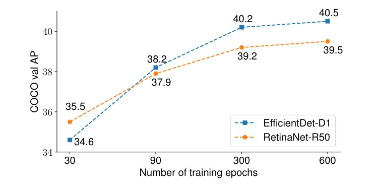
Figure 7: Accuracy vs. Training Epochs.

图 7：精度与训练轮数。

Training Epochs:

Many previous work only use a small number of epochs: for example, Detectron2 [1] trains each model with 12 epochs (1x schedule) in default, and at most 110 epochs (9x scahedule). Recent work [12] shows training longer is not helpful if using pretrained backbone networks; however, we observe training longer can significiantly improve accuracy in our settings. Figure 7 shows the performance comparison for different training epochs. We obseve: (1) both models benefit from longer training until reaching 300 epochs; (2) longer training is particularly important for EfficientDet, perhaps due to its small model size; (3) compared to the default 37 AP [24], our reproduced RetinaNet achieves higher accuracy (+2AP) using our training settings. In this paper, we mainly use 300 epochs for the good trade-off between accuracy and training time.

训练轮数：

已有工作往往只使用较少的训练轮数：例如，Detectron2 [1] 默认把每个模型训练 12 个轮次（1× 日程），最多 110 个轮次（9× 日程）。近期工作 [12] 表明，如果使用预训练的骨干网络，加长训练并无帮助；但在我们的设置里，加长训练可以明显提高精度。图 7 给出了不同训练轮数下的对比。我们观察到：（1）两种模型都能从更长的训练中获益，直到 300 个轮次；（2）加长训练对 EfficientDet 尤其重要，这可能是因为它的模型更小；（3）与默认的 37 AP [24] 相比，用我们的训练设置复现的 RetinaNet 精度更高（+2 AP）。本文主要采用 300 个轮次，以在精度和训练时间之间取得较好折中。

Scale Jittering:

A common training-time augmentation is to first resize images and then crop them into fixed size, known as scale jitterinig. Previous object detectors often use small jitters such as [0.8, 1.2], which randomly sample a scaling size between 0.8x to 1.2x of the original image size. However, we observe large jitters can improve accuracy if training longer. Figure 8 shows the results for different jitters: (1) when training with 30 epochs, a small jitter like [0.8, 1.2] performs quite good, and large jitters like [0.1, 2.0] actually hurts accuracy; (2) when training with 300 epochs, large jitters consistently improve accuracy, perhaps due to the stronger regularization. This paper uses a large jitter [0.1, 2.0] for all models.

尺度抖动：

一种常见的训练时增强，是先缩放图像再裁成固定大小，称为尺度抖动。已有检测器常用较小的抖动，例如 [0.8, 1.2]，即在原图尺寸的 0.8 倍到 1.2 倍之间随机采样缩放比例。但我们观察到，如果训练轮数足够长，较大的抖动反而能提高精度。图 8 给出了不同抖动设置的结果：（1）训练 30 个轮次时，像 [0.8, 1.2] 这样的小抖动表现较好，而 [0.1, 2.0] 这样的大抖动反而会损害精度；（2）训练 300 个轮次时，大抖动会稳定提高精度，这可能是因为正则更强。本文对所有模型都使用较大的抖动 [0.1, 2.0]。

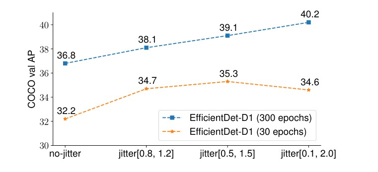
Figure 8: Accuracy vs. Scale Jittering.

图 8：精度与尺度抖动。

1.2 Image Resolutions

1.2 图像分辨率

In addition to our compound scaling that progressively increases image sizes, we are also interested in the accuracy-latency trade-offs with fixed image resolutions. Figure 9 compares EfficientDet-D1 to D6 with fixed and scaled resolutions. Surprisingly, their accuracy-latency trade-offs are very similar even though they have very different preferences: under similar accuracy constraints, models with fixed resolutions require much more parameters, but less activations and peak memory usage, than those with scaled resolutions. With fixed 640x640, our EfficientDet-D6 achieves real-time 47.9AP at 34ms latency.

除了按复合缩放逐步增大图像尺寸之外，我们也关心固定分辨率下的精度–延迟折中。图 9 比较了 EfficientDet-D1 到 D6 在固定分辨率和缩放分辨率下的结果。出乎意料的是，尽管二者偏好很不相同，精度–延迟折中却非常接近：在相近的精度约束下，固定分辨率的模型需要多得多的参数，但激活值和峰值显存占用更少。在固定的 640×640 下，我们的 EfficientDet-D6 以 34ms 延迟达到实时的 47.9 AP。

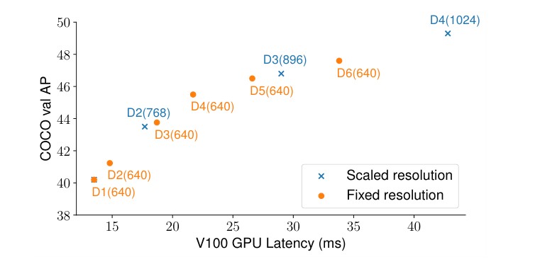
Figure 9: Comparison for Fixed and Scaled Resolution – fixed denotes 640x640 size and scaled denotes increased sizes.

图 9：固定分辨率与缩放分辨率的对比 – fixed 表示 640×640 的尺寸，scaled 表示按规则增大后的尺寸。