Dueling Network Architectures for Deep Reinforcement Learning
Dueling Network Architectures for Deep Reinforcement Learning
面向深度强化学习的对决网络结构
Ziyu Wang Tom Schaul Matteo Hessel Hado van Hasselt Marc Lanctot Nando de Freitas Address: Google DeepMind, London, UK
Abstract
摘要
In recent years there have been many successes of using deep representations in reinforcement learning. Still, many of these applications use conventional architectures, such as convolutional networks, LSTMs, or auto-encoders. In this paper, we present a new neural network architecture for model-free reinforcement learning. Our dueling network represents two separate estimators: one for the state value function and one for the state-dependent action advantage function. The main benefit of this factoring is to generalize learning across actions without imposing any change to the underlying reinforcement learning algorithm. Our results show that this architecture leads to better policy evaluation in the presence of many similar-valued actions. Moreover, the dueling architecture enables our RL agent to outperform the state-of-the-art on the Atari 2600 domain.
近年来,把深度表示用到强化学习中已经取得了许多成功。不过,这些应用里仍有不少使用的是常规结构,例如卷积网络、LSTM 或自编码器。本文为无模型强化学习提出一种新的神经网络结构。我们的对决网络表示两个分开的估计器:一个估计状态价值函数,一个估计依赖状态的动作优势函数。这种分解的主要好处,是在不必改动底层强化学习算法的前提下,让学习可以在不同动作之间推广。结果表明,当存在许多价值相近的动作时,这一结构能带来更好的策略评估。此外,对决结构使我们的强化学习智能体在 Atari 2600 领域超过了当时最好的方法。
1 Introduction
1 引言
Over the past years, deep learning has contributed to dramatic advances in scalability and performance of machine learning (LeCun et al., 2015). One exciting application is the sequential decision-making setting of reinforcement learning (RL) and control. Notable examples include deep Q-learning (Mnih et al., 2015), deep visuomotor policies (Levine et al., 2015), attention with recurrent networks (Ba et al., 2015), and model predictive control with embeddings (Watter et al., 2015). Other recent successes include massively parallel frameworks (Nair et al., 2015) and expert move prediction in the game of Go (Maddison et al., 2015), which produced policies matching those of Monte Carlo tree search programs, and squarely beaten a professional player when combined with search (Silver et al., 2016).
过去几年里,深度学习为机器学习的可扩展性和性能带来了显著进展(LeCun et al., 2015)。一个令人兴奋的应用,是强化学习(RL)与控制中的序贯决策设定。值得注意的例子包括深度 Q 学习(Mnih et al., 2015)、深度视觉运动策略(Levine et al., 2015)、带循环网络的注意力(Ba et al., 2015),以及用嵌入做模型预测控制(Watter et al., 2015)。其他近期的成功还包括大规模并行框架(Nair et al., 2015),以及围棋中的专家着法预测(Maddison et al., 2015)——后者产生的策略可以与蒙特卡洛树搜索程序相当,并在与搜索结合后清楚击败了一名职业棋手(Silver et al., 2016)。
In spite of this, most of the approaches for RL use standard neural networks, such as convolutional networks, MLPs, LSTMs and autoencoders. The focus in these recent advances has been on designing improved control and RL algorithms, or simply on incorporating existing neural network architectures into RL methods. Here, we take an alternative but complementary approach of focusing primarily on innovating a neural network architecture that is better suited for model-free RL. This approach has the benefit that the new network can be easily combined with existing and future algorithms for RL. That is, this paper advances a new network (Figure 1), but uses already published algorithms.
尽管如此,大多数强化学习方法使用的仍是标准神经网络,例如卷积网络、MLP、LSTM 和自编码器。这些近期进展的重点,是设计更好的控制与强化学习算法,或只是把已有的神经网络结构接入强化学习方法。这里,我们采取一种替代但互补的路径:把重点首先放在发明一种更适合无模型强化学习的神经网络结构上。这一路径的好处是,新网络可以很容易地与现有的以及未来的强化学习算法结合。也就是说,本文推进的是一种新网络(图 1),但使用的是已经发表的算法。
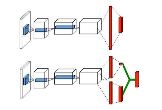
Figure 1: A popular single stream -network (top) and the dueling -network (bottom). The dueling network has two streams to separately estimate (scalar) state-value and the advantages for each action; the green output module implements equation (9) to combine them. Both networks output -values for each action.
图 1:一种常见的单流 网络(上)以及对决 网络(下)。对决网络有两条支路,分别估计(标量)状态价值和每个动作的优势;绿色输出模块实现式 (9) 来把它们组合起来。两种网络都输出每个动作的 值。
The proposed network architecture, which we name the dueling architecture, explicitly separates the representation of state values and (state-dependent) action advantages. The dueling architecture consists of two streams that represent the value and advantage functions, while sharing a common convolutional feature learning module. The two streams are combined via a special aggregating layer to produce an estimate of the state-action value function as shown in Figure 1. This dueling network should be understood as a single network with two streams that replaces the popular single-stream network in existing algorithms such as Deep Q-Networks (Mnih et al., 2015, DQN;). The dueling network automatically produces separate estimates of the state value function and advantage function, without any extra supervision.
我们所提出、并命名为对决结构(dueling architecture)的网络,显式地把状态价值的表示与(依赖状态的)动作优势的表示分开。对决结构由两条分别表示价值函数和优势函数的支路组成,同时共享一个公共的卷积特征学习模块。两条支路经过一层特殊的聚合层组合起来,得到状态–动作价值函数 的估计,如图 1 所示。这个对决网络应当被理解成一个带有两条支路的单一 网络,用来替换已有算法(例如 Deep Q-Networks(Mnih et al., 2015, DQN))中流行的单流 网络。对决网络会自动分别给出状态价值函数和优势函数的估计,而不需要任何额外的监督。
Intuitively, the dueling architecture can learn which states are (or are not) valuable, without having to learn the effect of each action for each state. This is particularly useful in states where its actions do not affect the environment in any relevant way. To illustrate this, consider the saliency maps shown in Figure 2[^1]. These maps were generated by computing the Jacobians of the trained value and advantage streams with respect to the input video, following the method proposed by Simonyan et al. (2013). (The experimental section describes this methodology in more detail.) The figure shows the value and advantage saliency maps for two different time steps. In one time step (leftmost pair of images), we see that the value network stream pays attention to the road and in particular to the horizon, where new cars appear. It also pays attention to the score. The advantage stream on the other hand does not pay much attention to the visual input because its action choice is practically irrelevant when there are no cars in front. However, in the second time step (rightmost pair of images) the advantage stream pays attention as there is a car immediately in front, making its choice of action very relevant.
直观上,对决结构可以学习哪些状态有(或没有)价值,而不必为每个状态学习每个动作的效果。这在动作不会以任何相关方式影响环境的那些状态里特别有用。为了说明这一点,请看图 2 中的显著性图(视频见 https://www.youtube.com/playlist?list=PLVFXyCSfS2Pau0gBh0mwTxDmutywWyFBP)。这些图是按照 Simonyan et al. (2013) 提出的方法,计算训练好的价值支路和优势支路对输入视频的雅可比得到的。(实验部分会更详细地描述这一方法。)该图给出了两个不同时间步上的价值和优势显著性图。在一个时间步(最左边的一对图像)里,我们看到价值网络支路关注路面,尤其是新车出现的地平线。它也关注分数。另一方面,优势支路对视觉输入关注不多,因为当前方没有车时,动作选择几乎无关紧要。然而在第二个时间步(最右边的一对图像)里,由于正前方已经有车,动作选择变得非常要紧,优势支路便开始关注。
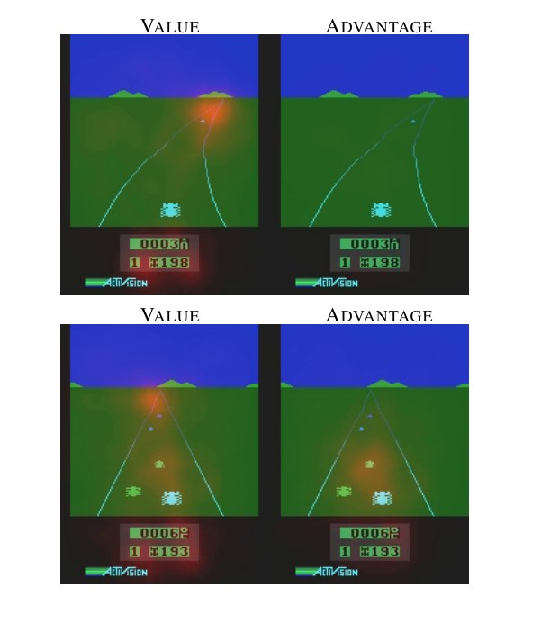
Figure 2: See, attend and drive: Value and advantage saliency maps (red-tinted overlay) on the Atari game Enduro, for a trained dueling architecture. The value stream learns to pay attention to the road. The advantage stream learns to pay attention only when there are cars immediately in front, so as to avoid collisions.
图 2:看、注意、再开车:在 Atari 游戏 Enduro 上,一个训练好的对决结构的价值和优势显著性图(红色调叠加)。价值支路学会关注路面。优势支路则学会只在正前方已有车辆、需要避免碰撞时才去关注。
In the experiments, we demonstrate that the dueling architecture can more quickly identify the correct action during policy evaluation as redundant or similar actions are added to the learning problem.
在实验中我们表明,当学习问题中加入冗余或相近的动作时,对决结构能在策略评估中更快地识别出正确动作。
We also evaluate the gains brought in by the dueling architecture on the challenging Atari 2600 testbed. Here, an RL agent with the same structure and hyper-parameters must be able to play 57 different games by observing image pixels and game scores only. The results illustrate vast improvements over the single-stream baselines of Mnih et al. (2015) and van Hasselt et al. (2015). The combination of prioritized replay (Schaul et al., 2016) with the proposed dueling network results in the new state-of-the-art for this popular domain.
我们也在具有挑战性的 Atari 2600 测试平台上评估了对决结构带来的增益。在这里,一个具有相同结构和超参数的强化学习智能体,必须只通过观察图像像素和游戏分数,就能玩 57 款不同的游戏。结果说明,它相对 Mnih et al. (2015) 和 van Hasselt et al. (2015) 的单流基线有大幅提升。把优先回放(Schaul et al., 2016)与所提出的对决网络结合起来,在这一流行领域得到了新的最好成绩。
1.1 Related Work
1.1 相关工作
The notion of maintaining separate value and advantage functions goes back to Baird (1993). In Baird’s original advantage updating algorithm, the shared Bellman residual update equation is decomposed into two updates: one for a state value function, and one for its associated advantage function. Advantage updating was shown to converge faster than Q-learning in simple continuous time domains in (Harmon et al., 1995). Its successor, the advantage learning algorithm, represents only a single advantage function (Harmon & Baird, 1996).
分别维护价值函数和优势函数这一想法,可以追溯到 Baird (1993)。在 Baird 最初的优势更新算法里,共享的 Bellman 残差更新方程被分解成两次更新:一次针对状态价值函数,一次针对与之相伴的优势函数。Harmon et al. (1995) 表明,在简单的连续时间域上,优势更新比 Q 学习收敛更快。它的后继——优势学习算法——只表示单个优势函数(Harmon & Baird, 1996)。
The dueling architecture represents both the value and advantage functions with a single deep model whose output combines the two to produce a state-action value . Unlike in advantage updating, the representation and algorithm are decoupled by construction. Consequently, the dueling architecture can be used in combination with a myriad of model free RL algorithms.
对决结构用一个单一的深度模型同时表示价值 和优势 函数,其输出把二者组合起来,得到状态–动作价值 。与优势更新不同,表示和算法在构造上是解耦的。因此,对决结构可以与众多无模型强化学习算法结合使用。
There is a long history of advantage functions in policy gradients, starting with (Sutton et al., 2000). As a recent example of this line of work, Schulman et al. (2015) estimate advantage values online to reduce the variance of policy gradient algorithms.
优势函数在策略梯度中有很长的历史,始于 (Sutton et al., 2000)。作为这条线上的一个近期例子,Schulman et al. (2015) 在线估计优势值,以降低策略梯度算法的方差。
There have been several attempts at playing Atari with deep reinforcement learning, including Mnih et al. (2015); Guo et al. (2014); Stadie et al. (2015); Nair et al. (2015); van Hasselt et al. (2015); Bellemare et al. (2016) and Schaul et al. (2016). The results of Schaul et al. (2016) are the current published state-of-the-art.
用深度强化学习玩 Atari 已有若干尝试,包括 Mnih et al. (2015);Guo et al. (2014);Stadie et al. (2015);Nair et al. (2015);van Hasselt et al. (2015);Bellemare et al. (2016) 以及 Schaul et al. (2016)。Schaul et al. (2016) 的结果是当时已发表的最好成绩。
2 Background
2 背景
We consider a sequential decision making setup, in which an agent interacts with an environment over discrete time steps, see Sutton & Barto (1998) for an introduction. In the Atari domain, for example, the agent perceives a video consisting of image frames: at time step . The agent then chooses an action from a discrete set and observes a reward signal produced by the game emulator.
我们考虑一个序贯决策设定:智能体在离散时间步上与环境 交互,入门介绍见 Sutton & Barto (1998)。例如在 Atari 领域,智能体在时间步 感知由 帧图像组成的视频 :。智能体随后从离散集合 中选择一个动作,并观察到由游戏模拟器产生的奖励信号 。
The agent seeks maximize the expected discounted return, where we define the discounted return as . In this formulation, is a discount factor that trades-off the importance of immediate and future rewards.
智能体寻求最大化期望折现回报,其中我们把折现回报定义为 。在这一表述中, 是一个折现因子,用来权衡即时奖励与未来奖励的重要性。
For an agent behaving according to a stochastic policy , the values of the state-action pair and the state are defined as follows
对于一个按照随机策略 行动的智能体,状态–动作对 以及状态 的价值定义如下
The preceding state-action value function ( function for short) can be computed recursively with dynamic programming:
前面的状态–动作价值函数(简称 函数)可以用动态规划递归计算:
We define the optimal Under the deterministic policy , it follows that From this, it also follows that the optimal function satisfies the Bellman equation:
我们定义最优 在确定性策略 下,随之有 由此也可知,最优 函数满足 Bellman 方程:
We define another important quantity, the advantage function, relating the value and functions:
我们再定义一个重要的量,即把价值函数和 函数联系起来的优势函数:
Note that . Intuitively, the value function measures the how good it is to be in a particular state . The function, however, measures the the value of choosing a particular action when in this state. The advantage function subtracts the value of the state from the Q function to obtain a relative measure of the importance of each action.
注意 。直观上,价值函数 衡量处在某个特定状态 有多好。而 函数衡量的是在这个状态选择某个特定动作的价值。优势函数从 函数中减去状态的价值,从而得到每个动作相对重要性的度量。
2.1 Deep Q-networks
2.1 深度 Q 网络
The value functions as described in the preceding section are high dimensional objects. To approximate them, we can use a deep -network: with parameters . To estimate this network, we optimize the following sequence of loss functions at iteration :
前一节所描述的价值函数是高维对象。为了近似它们,我们可以使用带参数 的深度 网络:。为了估计这个网络,我们在第 次迭代优化如下损失序列:
with
其中
where represents the parameters of a fixed and separate target network. We could attempt to use standard -learning to learn the parameters of the network online. However, this estimator performs poorly in practice. A key innovation in (Mnih et al., 2015) was to freeze the parameters of the target network for a fixed number of iterations while updating the online network by gradient descent. (This greatly improves the stability of the algorithm.) The specific gradient update is
这里 表示一个固定且分开的目标网络的参数。我们也可以尝试用标准 学习在线学习网络 的参数。不过这个估计器在实践中表现很差。(Mnih et al., 2015) 中的一项关键创新,是在用梯度下降更新在线网络 时,把目标网络 的参数冻结固定的迭代次数。(这大大提高了算法的稳定性。)具体的梯度更新是
This approach is model free in the sense that the states and rewards are produced by the environment. It is also off-policy because these states and rewards are obtained with a behavior policy (epsilon greedy in DQN) different from the online policy that is being learned.
这一方法是无模型的,因为状态和奖励由环境产生。它也是离策略的,因为这些状态和奖励是用一种行为策略(DQN 中是 -贪心)得到的,而该行为策略不同于正在学习的在线策略。
Another key ingredient behind the success of DQN is experience replay (Lin, 1993; Mnih et al., 2015). During learning, the agent accumulates a dataset of experiences from many episodes. When training the -network, instead only using the current experience as prescribed by standard temporal-difference learning, the network is trained by sampling mini-batches of experiences from uniformly at random. The sequence of losses thus takes the form
DQN 成功背后的另一项关键成分是经验回放(Lin, 1993; Mnih et al., 2015)。学习过程中,智能体从许多回合里积累一个经验数据集 ,其中 。训练 网络时,并不像标准时序差分学习所规定的那样只用当前经验,而是从 中均匀随机采样经验小批量来训练网络。于是损失序列取如下形式
Experience replay increases data efficiency through re-use of experience samples in multiple updates and, importantly, it reduces variance as uniform sampling from the replay buffer reduces the correlation among the samples used in the update.
经验回放通过在多次更新中重复使用经验样本来提高数据效率;更重要的是,它降低了方差,因为从回放缓冲里均匀采样减少了更新所用样本之间的相关性。
2.2 Double Deep Q-networks
2.2 双重深度 Q 网络
The previous section described the main components of DQN as presented in (Mnih et al., 2015). In this paper, we use the improved Double DQN (DDQN) learning algorithm of van Hasselt et al. (2015). In Q-learning and DQN, the operator uses the same values to both select and evaluate an action. This can therefore lead to overoptimistic value estimates (van Hasselt, 2010). To mitigate this problem, DDQN uses the following target:
上一节描述了 (Mnih et al., 2015) 中给出的 DQN 主要成分。本文使用 van Hasselt et al. (2015) 改进后的双重 DQN(DDQN)学习算法。在 Q 学习和 DQN 中, 算子用同一组值既选择动作又评估动作。因此这可能导致过于乐观的价值估计(van Hasselt, 2010)。为缓解这一问题,DDQN 使用如下目标:
DDQN is the same as for DQN (see Mnih et al. (2015)), but with the target replaced by . The pseudo-code for DDQN is presented in Appendix A.
DDQN 与 DQN 相同(见 Mnih et al. (2015)),只是把目标 换成 。DDQN 的伪代码见附录 A。
2.3 Prioritized Replay
2.3 优先回放
A recent innovation in prioritized experience replay (Schaul et al., 2016) built on top of DDQN and further improved the state-of-the-art. Their key idea was to increase the replay probability of experience tuples that have a high expected learning progress (as measured via the proxy of absolute TD-error). This led to both faster learning and to better final policy quality across most games of the Atari benchmark suite, as compared to uniform experience replay.
优先经验回放(Schaul et al., 2016)是建立在 DDQN 之上的一项近期创新,并进一步刷新了当时最好的成绩。他们的关键想法是,提高那些预期学习进度高(以绝对 TD 误差作为代理来衡量)的经验元组的回放概率。与均匀经验回放相比,这在 Atari 基准套件的大多数游戏上既加快了学习,也提高了最终策略质量。
To strengthen the claim that our dueling architecture is complementary to algorithmic innovations, we show that it improves performance for both the uniform and the prioritized replay baselines (for which we picked the easier to implement rank-based variant), with the resulting prioritized dueling variant holding the new state-of-the-art.
为了加强“对决结构与算法创新是互补的”这一论断,我们表明,它对均匀回放和优先回放两种基线都能提高表现(优先回放我们选用了更容易实现的基于秩的变体),由此得到的优先对决变体保持了新的最好成绩。
3 The Dueling Network Architecture
3 对决网络结构
The key insight behind our new architecture, as illustrated in Figure 2, is that for many states, it is unnecessary to estimate the value of each action choice. For example, in the Enduro game setting, knowing whether to move left or right only matters when a collision is eminent. In some states, it is of paramount importance to know which action to take, but in many other states the choice of action has no repercussion on what happens. For bootstrapping based algorithms, however, the estimation of state values is of great importance for every state.
如图 2 所说明的,我们这一新结构背后的关键认识是:对许多状态来说,没有必要估计每个动作选择的价值。例如在 Enduro 这款游戏的设定里,只有在碰撞即将发生时,知道该向左还是向右才要紧。在有些状态里,知道该采取哪个动作至关重要,但在许多其他状态里,动作选择对接下来发生的事没有影响。不过,对于基于自举的算法,每个状态上的状态价值估计都非常重要。
To bring this insight to fruition, we design a single -network architecture, as illustrated in Figure 1, which we refer to as the dueling network. The lower layers of the dueling network are convolutional as in the original DQNs (Mnih et al., 2015). However, instead of following the convolutional layers with a single sequence of fully connected layers, we instead use two sequences (or streams) of fully connected layers. The streams are constructed such that they have they have the capability of providing separate estimates of the value and advantage functions. Finally, the two streams are combined to produce a single output function. As in (Mnih et al., 2015), the output of the network is a set of values, one for each action.
为了把这一认识落到实处,我们设计了如图 1 所示的单一 网络结构,并把它称为对决网络。对决网络的较低层与原先的 DQN 一样是卷积(Mnih et al., 2015)。不过,在卷积层之后我们不再接单一的一串全连接层,而是使用两串(或者说两条支路)全连接层。这两条支路被构造成能够分别提供价值函数和优势函数的估计。最后,两条支路组合起来,产生单一的输出 函数。与 (Mnih et al., 2015) 一样,网络的输出是一组 值,每个动作一个。
Since the output of the dueling network is a function, it can be trained with the many existing algorithms, such as DDQN and SARSA. In addition, it can take advantage of any improvements to these algorithms, including better replay memories, better exploration policies, intrinsic motivation, and so on.
因为对决网络的输出是一个 函数,它可以用许多已有算法来训练,例如 DDQN 和 SARSA。此外,它也可以利用这些算法的任何改进,包括更好的回放记忆、更好的探索策略、内在动机等等。
The module that combines the two streams of fully-connected layers to output a estimate requires very thoughtful design.
把两条全连接支路组合起来、输出 估计的那个模块,需要非常审慎的设计。
From the expressions for advantage and state-value , it follows that . Moreover, for a deterministic policy, , it follows that and hence .
由优势的表达式 以及状态价值 ,可以推出 。此外,对于确定性策略 ,有 ,从而 。
Let us consider the dueling network shown in Figure 1, where we make one stream of fully-connected layers output a scalar , and the other stream output an -dimensional vector . Here, denotes the parameters of the convolutional layers, while and are the parameters of the two streams of fully-connected layers.
让我们考虑图 1 所示的对决网络:我们让一条全连接支路输出标量 ,另一条支路输出一个 维向量 。这里, 表示卷积层的参数,而 和 是两条全连接支路的参数。
Using the definition of advantage, we might be tempted to construct the aggregating module as follows:
利用优势的定义,我们可能会想把聚合模块构造成如下形式:
Note that this expression applies to all instances; that is, to express equation (7) in matrix form we need to replicate the scalar, , times.
注意这一表达式适用于所有 实例;也就是说,要把式 (7) 写成矩阵形式,需要把标量 复制 次。
However, we need to keep in mind that is only a parameterized estimate of the true -function. Moreover, it would be wrong to conclude that is a good estimator of the state-value function, or likewise that provides a reasonable estimate of the advantage function.
不过需要记住, 只是对真正 函数的参数化估计。此外,不能由此断定 就是状态价值函数的好估计器,同样也不能断定 就提供了优势函数的合理估计。
Equation (7) is unidentifiable in the sense that given we cannot recover and uniquely. To see this, add a constant to and subtract the same constant from . This constant cancels out resulting in the same value. This lack of identifiability is mirrored by poor practical performance when this equation is used directly.
式 (7) 在如下意义上是不可辨识的:给定 ,我们无法唯一还原 和 。只要给 加上一个常数,再从 中减去同一个常数,就能看出这一点。这个常数相互抵消,得到的 值不变。这种缺乏可辨识性,也反映在直接使用该式时实践表现很差。
To address this issue of identifiability, we can force the advantage function estimator to have zero advantage at the chosen action. That is, we let the last module of the network implement the forward mapping
为了解决这一可辨识性问题,我们可以迫使优势函数估计器在所选定的动作上优势为零。也就是说,我们让网络的最后一个模块实现如下前向映射
$$Q(s,a;\theta,\alpha,\beta)={V}(s;\theta,\beta)~+\
\left({A}(s,a;\theta,\alpha)-\max_{a^{\prime}\in|\mathcal{A}|}{A}(s,a^{\prime};\theta,\alpha)\right). \tag{8}$$
Now, for , we obtain . Hence, the stream provides an estimate of the value function, while the other stream produces an estimate of the advantage function.
于是,对 ,我们得到 。因此,支路 提供价值函数的估计,另一条支路则产生优势函数的估计。
An alternative module replaces the max operator with an average:
另一种模块是把 max 算子换成平均:
$$Q(s,a;\theta,\alpha,\beta)={V}(s;\theta,\beta)~+\
\left({A}(s,a;\theta,\alpha)-\frac{1}{|\mathcal{A}|}\sum_{a^{\prime}}{A}(s,a^{\prime};\theta,\alpha)\right). \tag{9}$$
On the one hand this loses the original semantics of and because they are now off-target by a constant, but on the other hand it increases the stability of the optimization: with (9) the advantages only need to change as fast as the mean, instead of having to compensate any change to the optimal action’s advantage in (8). We also experimented with a softmax version of equation (8), but found it to deliver similar results to the simpler module of equation (9). Hence, all the experiments reported in this paper use the module of equation (9).
一方面,这会失去 和 原先的语义,因为它们现在会偏离一个常数;另一方面,它提高了优化的稳定性:在 (9) 中,优势只需与均值一样快地变化,而不必像 (8) 那样去补偿最优动作优势上的任何变化。我们也实验过式 (8) 的一种 softmax 版本,但发现它与更简单的式 (9) 模块给出相近的结果。因此,本文报告的全部实验都使用式 (9) 的模块。
Note that while subtracting the mean in equation (9) helps with identifiability, it does not change the relative rank of the (and hence ) values, preserving any greedy or -greedy policy based on values from equation (7). When acting, it suffices to evaluate the advantage stream to make decisions.
需要注意的是,虽然在式 (9) 中减去均值有助于可辨识性,它并不改变 (从而也不改变 )值的相对排序,因此基于式 (7) 的 值的任何贪心或 -贪心策略都得以保留。在行动时,只需评估优势支路就可以做决策。
It is important to note that equation (9) is viewed and implemented as part of the network and not as a separate algorithmic step. Training of the dueling architectures, as with standard networks (e.g. the deep -network of Mnih et al. (2015)), requires only back-propagation. The estimates and are computed automatically without any extra supervision or algorithmic modifications.
重要的是,式 (9) 被看成并实现为网络的一部分,而不是一个单独的算法步骤。与标准 网络(例如 Mnih et al. (2015) 的深度 网络)一样,训练对决结构只需要反向传播。估计 和 会自动算出来,不需要任何额外的监督或算法修改。
As the dueling architecture shares the same input-output interface with standard networks, we can recycle all learning algorithms with networks (e.g., DDQN and SARSA) to train the dueling architecture.
由于对决结构与标准 网络共享相同的输入–输出接口,我们可以把所有带 网络的学习算法(例如 DDQN 和 SARSA)重新用来训练对决结构。
4 Experiments
4 实验
We now show the practical performance of the dueling network. We start with a simple policy evaluation task and then show larger scale results for learning policies for general Atari game-playing.
我们现在展示对决网络的实际表现。我们先从一个简单的策略评估任务开始,再给出在一般 Atari 游戏对局中学习策略的更大规模结果。
4.1 Policy evaluation
4.1 策略评估
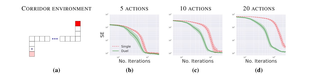
Figure 3: (a) The corridor environment. The star marks the starting state. The redness of a state signifies the reward the agent receives upon arrival. The game terminates upon reaching either reward state. The agent’s actions are going up, down, left, right and no action. Plots (b), (c) and (d) shows squared error for policy evaluation with 5, 10, and 20 actions on a log-log scale. The dueling network (Duel) consistently outperforms a conventional single-stream network (Single), with the performance gap increasing with the number of actions.
图 3:(a) 走廊环境。星号标出起始状态。某个状态的红色程度表示智能体到达该状态时所获得的奖励。游戏在到达任一奖励状态时终止。智能体的动作是向上、向下、向左、向右以及不动。图 (b)、(c) 和 (d) 在双对数坐标上给出动作数为 5、10 和 20 时策略评估的平方误差。对决网络(Duel)始终超过常规的单流网络(Single),而且表现差距随动作数增大而变大。
We start by measuring the performance of the dueling architecture on a policy evaluation task. We choose this particular task because it is very useful for evaluating network architectures, as it is devoid of confounding factors such as the choice of exploration strategy, and the interaction between policy improvement and policy evaluation.
我们先在一个策略评估任务上衡量对决结构的表现。选择这一特定任务,是因为它对评估网络结构非常有用:它没有探索策略选择、以及策略改进与策略评估之间相互作用这类混杂因素。
In this experiment, we employ temporal difference learning (without eligibility traces, i.e., ) to learn values. More specifically, given a behavior policy , we seek to estimate the state-action value by optimizing the sequence of costs of equation (4), with target
在这一实验中,我们采用时序差分学习(不带资格迹,即 )来学习 值。更具体地说,给定行为策略 ,我们通过优化式 (4) 的代价序列来估计状态–动作价值 ,其目标为
The above update rule is the same as that of Expected SARSA (van Seijen et al., 2009). We, however, do not modify the behavior policy as in Expected SARSA.
上述更新规则与 Expected SARSA(van Seijen et al., 2009)相同。不过我们并不像 Expected SARSA 那样修改行为策略。
To evaluate the learned values, we choose a simple environment where the exact values can be computed separately for all . This environment, which we call the corridor is composed of three connected corridors. A schematic drawing of the corridor environment is shown in Figure 3, The agent starts from the bottom left corner of the environment and must move to the top right to get the largest reward. A total of actions are available: go up, down, left, right and no-op. We also have the freedom of adding an arbitrary number of no-op actions. In our setup, the two vertical sections both have 10 states while the horizontal section has 50.
为了评估学到的 值,我们选择一个可以对所有 单独算出精确 值的简单环境。这个我们称之为走廊的环境,由三段相连的走廊组成。走廊环境的示意画法见图 3。智能体从环境的左下角出发,必须走到右上角才能获得最大奖励。一共有 个可用动作:向上、向下、向左、向右以及空操作。我们也可以自由加入任意数量的空操作动作。在我们的设置里,两段竖直部分都有 10 个状态,水平部分有 50 个状态。
We use an -greedy policy as the behavior policy , which chooses a random action with probability or an action according to the optimal function with probability . In our experiments, is chosen to be .
我们使用 -贪心策略作为行为策略 ,它以概率 选择随机动作,或以概率 按照最优 函数 选择动作。实验中 取为 。
We compare a single-stream architecture with the dueling architecture on three variants of the corridor environment with 5, 10 and 20 actions respectively. The 10 and 20 action variants are formed by adding no-ops to the original environment. We measure performance by Squared Error (SE) against the true state values: . The single-stream architecture is a three layer MLP with units on each hidden layer. The dueling architecture is also composed of three layers. After the first hidden layer of 50 units, however, the network branches off into two streams each of them a two layer MLP with 25 hidden units. The results of the comparison are summarized in Figure 3.
我们在走廊环境的三个变体上比较单流 结构与对决结构,动作数分别为 5、10 和 20。10 和 20 个动作的变体,是通过向原环境加入空操作形成的。我们用相对真实状态价值的平方误差(SE)来衡量表现:。单流结构是一个三层 MLP,每个隐层有 个单元。对决结构同样由三层组成。不过在 50 个单元的第一个隐层之后,网络分成两条支路,每条都是带 25 个隐单元的两层 MLP。比较结果汇总在图 3 中。
The results show that with actions, both architectures converge at about the same speed. However, when we increase the number of actions, the dueling architecture performs better than the traditional -network. In the dueling network, the stream learns a general value that is shared across many similar actions at , hence leading to faster convergence. This is a very promising result because many control tasks with large action spaces have this property, and consequently we should expect that the dueling network will often lead to much faster convergence than a traditional single stream network. In the following section, we will indeed see that the dueling network results in substantial gains in performance in a wide-range of Atari games.
结果表明,在 个动作时,两种结构以大致相同的速度收敛。然而当我们增加动作数时,对决结构的表现优于传统 网络。在对决网络中,支路 学到一个在 上许多相近动作之间共享的一般价值,因而带来更快的收敛。这是一个很有希望的结果,因为许多具有大动作空间的控制任务都有这一性质,因此我们应当预期,对决网络往往会比传统的单流网络收敛得快得多。在下一节里,我们的确会看到,对决网络在范围很广的 Atari 游戏上带来了可观的表现提升。
4.2 General Atari Game-Playing
4.2 一般的 Atari 游戏对局
We perform a comprehensive evaluation of our proposed method on the Arcade Learning Environment (Bellemare et al., 2013), which is composed of 57 Atari games. The challenge is to deploy a single algorithm and architecture, with a fixed set of hyper-parameters, to learn to play all the games given only raw pixel observations and game rewards. This environment is very demanding because it is both comprised of a large number of highly diverse games and the observations are high-dimensional.
我们在由 57 款 Atari 游戏组成的 Arcade Learning Environment(Bellemare et al., 2013)上,对所提出的方法做了全面评估。挑战在于部署同一套算法和结构、使用固定的一组超参数,只根据原始像素观测和游戏奖励,学会玩所有游戏。这一环境要求很高,因为它既包含大量彼此差异很大的游戏,观测又是高维的。
We follow closely the setup of van Hasselt et al. (2015) and compare to their results using single-stream -networks. We train the dueling network with the DDQN algorithm as presented in Appendix A. At the end of this section, we incorporate prioritized experience replay (Schaul et al., 2016).
我们尽量沿用 van Hasselt et al. (2015) 的设置,并与他们使用单流 网络的结果做比较。我们用附录 A 中给出的 DDQN 算法训练对决网络。在本节末尾,我们再引入优先经验回放(Schaul et al., 2016)。
Our network architecture has the same low-level convolutional structure of DQN (Mnih et al., 2015; van Hasselt et al., 2015). There are 3 convolutional layers followed by 2 fully-connected layers. The first convolutional layer has 32 filters with stride 4, the second 64 filters with stride 2, and the third and final convolutional layer consists 64 filters with stride 1. As shown in Figure 1, the dueling network splits into two streams of fully connected layers. The value and advantage streams both have a fully-connected layer with 512 units. The final hidden layers of the value and advantage streams are both fully-connected with the value stream having one output and the advantage as many outputs as there are valid actions[^2]. We combine the value and advantage streams using the module described by Equation (9). Rectifier non-linearities (Fukushima, 1980) are inserted between all adjacent layers.
我们的网络结构具有与 DQN 相同的低层卷积结构(Mnih et al., 2015; van Hasselt et al., 2015)。共有 3 个卷积层,后面再接 2 个全连接层。第一个卷积层有 32 个步幅为 4 的 滤波器,第二个有 64 个步幅为 2 的 滤波器,第三个也是最后一个卷积层由 64 个步幅为 1 的 滤波器组成。如图 1 所示,对决网络分成两条全连接支路。价值支路和优势支路都有一个 512 个单元的全连接层。价值支路和优势支路的最后隐层也都是全连接的,价值支路有一个输出,优势支路的输出数与合法动作数相同(ALE 环境中的动作数在 3 到 18 之间)。我们用式 (9) 所描述的模块来组合价值支路和优势支路。在所有相邻层之间插入整流非线性(Fukushima, 1980)。
We adopt the optimizers and hyper-parameters of van Hasselt et al. (2015), with the exception of the learning rate which we chose to be slightly lower (we do not do this for double DQN as it can deteriorate its performance). Since both the advantage and the value stream propagate gradients to the last convolutional layer in the backward pass, we rescale the combined gradient entering the last convolutional layer by . This simple heuristic mildly increases stability. In addition, we clip the gradients to have their norm less than or equal to 10. This clipping is not standard practice in deep RL, but common in recurrent network training (Bengio et al., 2013).
我们采用 van Hasselt et al. (2015) 的优化器和超参数,只是把学习率选得略低一些(对双重 DQN 我们不做这一改动,因为它可能损害其表现)。由于优势支路和价值支路在反向传播时都会把梯度传到最后一个卷积层,我们把进入最后一个卷积层的组合梯度按 重新缩放。这一简单的启发式略微提高了稳定性。此外,我们把梯度裁剪到范数不超过 10。这种裁剪在深度强化学习中并非标准做法,但在循环网络训练中很常见(Bengio et al., 2013)。
To isolate the contributions of the dueling architecture, we re-train DDQN with a single stream network using exactly the same procedure as described above. Specifically, we apply gradient clipping, and use hidden units for the first fully-connected layer of the network so that both architectures (dueling and single) have roughly the same number of parameters. We refer to this re-trained model as Single Clip, while the original trained model of van Hasselt et al. (2015) is referred to as Single.
为了分离对决结构的贡献,我们用完全相同的上述规程,重新训练了一个单流网络的 DDQN。具体地说,我们施加梯度裁剪,并把网络第一个全连接层设为 个隐单元,使两种结构(对决与单流)具有大致相同的参数量。我们把这个重新训练的模型称为 Single Clip,而把 van Hasselt et al. (2015) 原先训练的模型称为 Single。
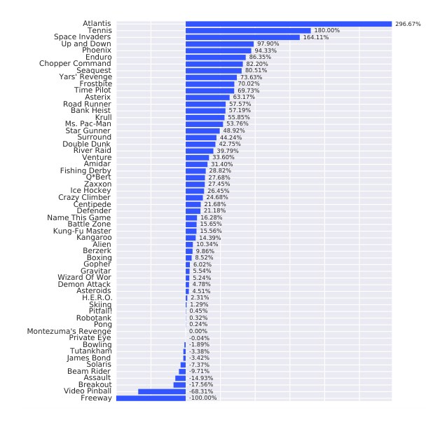
Figure 4: Improvements of dueling architecture over the baseline Single network of van Hasselt et al. (2015), using the metric described in Equation (10). Bars to the right indicate by how much the dueling network outperforms the single-stream network.
图 4:对决结构相对 van Hasselt et al. (2015) 的基线 Single 网络的改进,所用度量见式 (10)。向右的条形表示对决网络超出单流网络的幅度。
As in (van Hasselt et al., 2015), we start the game with up to 30 no-op actions to provide random starting positions for the agent. To evaluate our approach, we measure improvement in percentage (positive or negative) in score over the better of human and baseline agent scores:
与 (van Hasselt et al., 2015) 一样,我们在开局时加入最多 30 步空操作,以便为智能体提供随机的起始位置。为评估方法,我们衡量分数相对人类与基线智能体分数中较好者的百分比改进(可正可负):
We took the maximum over human and baseline agent scores as it prevents insignificant changes to appear as large improvements when neither the agent in question nor the baseline are doing well. For example, an agent that achieves 2% human performance should not be interpreted as two times better when the baseline agent achieves 1% human performance. We also chose not to measure performance in terms of percentage of human performance alone because a tiny difference relative to the baseline on some games can translate into hundreds of percent in human performance difference.
我们在人类分数和基线智能体分数上取最大值,是为了避免在所讨论的智能体和基线都表现不佳时,把微不足道的变化看成大幅改进。例如,一个达到 2% 人类水平的智能体,在基线智能体达到 1% 人类水平时,不应被解释成好了两倍。我们也选择不只按人类水平百分比来衡量表现,因为某些游戏上相对基线的微小差别,可以转化成数百个百分点的人类水平差距。
The results for the wide suite of 57 games are summarized in Table 1. Detailed results are presented in the Appendix.
57 款游戏这一大套结果汇总在表 1 中。详细结果见附录。
Using this 30 no-ops performance measure, it is clear that the dueling network (Duel Clip) does substantially better than the Single Clip network of similar capacity. It also does considerably better than the baseline (Single) of van Hasselt et al. (2015). For comparison we also show results for the deep -network of Mnih et al. (2015), referred to as Nature DQN.
用这一 30 步空操作的表现度量可以清楚地看到,对决网络(Duel Clip)明显好于容量相近的 Single Clip 网络。它也明显好于 van Hasselt et al. (2015) 的基线(Single)。作为对照,我们也给出 Mnih et al. (2015) 的深度 网络结果,称为 Nature DQN。
Figure 4 shows the improvement of the dueling network over the baseline Single network of van Hasselt et al. (2015). Again, we seen that the improvements are often very dramatic.
图 4 给出对决网络相对 van Hasselt et al. (2015) 的基线 Single 网络的改进。我们再次看到,这些改进往往非常显著。
As shown in Table 1, Single Clip performs better than Single. We verified that this gain was mostly brought in by gradient clipping. For this reason, we incorporate gradient clipping in all the new approaches.
如表 1 所示,Single Clip 的表现好于 Single。我们核过,这一增益主要来自梯度裁剪。因此,我们在所有新方法中都加入了梯度裁剪。
| 30 no-ops | Human Starts | |||
|---|---|---|---|---|
| Mean | Median | Mean | Median | |
| Prior. Duel Clip | 591.9% | 172.1% | 567.0% | 115.3% |
| Prior. Single | 434.6% | 123.7% | 386.7% | 112.9% |
| Duel Clip | 373.1% | 151.5% | 343.8% | 117.1% |
| Single Clip | 341.2% | 132.6% | 302.8% | 114.1% |
| Single | 307.3% | 117.8% | 332.9% | 110.9% |
| Nature DQN | 227.9% | 79.1% | 219.6% | 68.5% |
Table 1: Mean and median scores across all 57 Atari games, measured in percentages of human performance.
| 30 no-ops | Human Starts | |||
|---|---|---|---|---|
| Mean | Median | Mean | Median | |
| Prior. Duel Clip | 591.9% | 172.1% | 567.0% | 115.3% |
| Prior. Single | 434.6% | 123.7% | 386.7% | 112.9% |
| Duel Clip | 373.1% | 151.5% | 343.8% | 117.1% |
| Single Clip | 341.2% | 132.6% | 302.8% | 114.1% |
| Single | 307.3% | 117.8% | 332.9% | 110.9% |
| Nature DQN | 227.9% | 79.1% | 219.6% | 68.5% |
表 1:全部 57 款 Atari 游戏上的均值和中位数分数,以人类水平的百分比衡量。
Duel Clip does better than Single Clip on 75.4% of the games (43 out of 57). It also achieves higher scores compared to the Single baseline on 80.7% ( out of ) of the games. Of all the games with actions, Duel Clip is better % of the time (26 out of 30). This is consistent with the findings of the previous section. Overall, our agent (Duel Clip) achieves human level performance on 42 out of 57 games. Raw scores for all the games, as well as measurements in human performance percentage, are presented in the Appendix.
Duel Clip 在 75.4% 的游戏上好于 Single Clip(57 款中的 43 款)。相对 Single 基线,它也在 80.7%( 款中的 款)的游戏上取得更高分数。在全部有 个动作的游戏里,Duel Clip 有 % 的时候更好(30 款中的 26 款)。这与上一节的发现是一致的。总体上看,我们的智能体(Duel Clip)在 57 款游戏中的 42 款上达到了人类水平。全部游戏的原始分数,以及按人类水平百分比衡量的结果,见附录。
Robustness to human starts. One shortcoming of the 30 no-ops metric is that an agent does not necessarily have to generalize well to play the Atari games. Due to the deterministic nature of the Atari environment, from an unique starting point, an agent could learn to achieve good performance by simply remembering sequences of actions.
对人类起点的稳健性。 30 步空操作这一指标的一个不足,是智能体不一定需要很好地推广就能玩 Atari 游戏。由于 Atari 环境是确定性的,从一个唯一的起点出发,智能体可能只靠记住动作序列就学到不错的表现。
To obtain a more robust measure, we adopt the methodology of Nair et al. (2015). Specifically, for each game, we use 100 starting points sampled from a human expert’s trajectory. From each of these points, an evaluation episode is launched for up to 108,000 frames. The agents are evaluated only on rewards accrued after the starting point. We refer to this metric as Human Starts.
为了得到更稳健的度量,我们采用 Nair et al. (2015) 的方法。具体地说,对每款游戏,我们从一位人类专家的轨迹中采样 100 个起点。从这些点中的每一个出发,启动一个最多 108,000 帧的评测回合。智能体只按起点之后累积的奖励来评测。我们把这一指标称为 Human Starts(人类起点)。
As shown in Table 1, under the Human Starts metric, Duel Clip once again outperforms the single stream variants. In particular, our agent does better than the Single baseline on 70.2% (40 out of 57) games and on games of actions, Duel Clip is 83.3% better (25 out of 30).
如表 1 所示,在 Human Starts 指标下,Duel Clip 再次超过单流变体。特别是,我们的智能体在 70.2%(57 款中的 40 款)的游戏上好于 Single 基线;在有 个动作的游戏上,Duel Clip 好于基线的比例是 83.3%(30 款中的 25 款)。
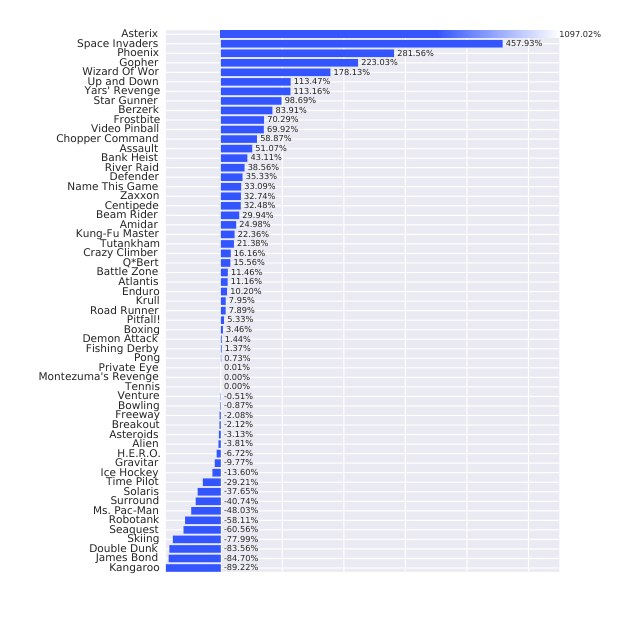
Figure 5: Improvements of dueling architecture over Prioritized DDQN baseline, using the same metric as Figure 4. Again, the dueling architecture leads to significant improvements over the single-stream baseline on the majority of games.
图 5:对决结构相对优先 DDQN 基线的改进,所用度量与图 4 相同。对决结构再次在大多数游戏上相对单流基线带来显著改进。
Combining with Prioritized Experience Replay. The dueling architecture can be easily combined with other algorithmic improvements. In particular, prioritization of the experience replay has been shown to significantly improve performance of Atari games (Schaul et al., 2016). Furthermore, as prioritization and the dueling architecture address very different aspects of the learning process, their combination is promising. So in our final experiment, we investigate the integration of the dueling architecture with prioritized experience replay. We use the prioritized variant of DDQN (Prior. Single) as the new baseline algorithm, which replaces with the uniform sampling of the experience tuples by rank-based prioritized sampling. We keep all the parameters of the prioritized replay as described in (Schaul et al., 2016), namely a priority exponent of , and an annealing schedule on the importance sampling exponent from to . We combine this baseline with our dueling architecture (as above), and again use gradient clipping (Prior. Duel Clip).
与优先经验回放结合。 对决结构可以很容易地与其他算法改进结合起来。特别是,经验回放的优先化已被表明能显著提高 Atari 游戏上的表现(Schaul et al., 2016)。此外,由于优先化与对决结构处理的是学习过程中非常不同的方面,把它们结合起来是有希望的。因此在最后一项实验里,我们考察把对决结构与优先经验回放整合在一起。我们把 DDQN 的优先变体(Prior. Single)作为新的基线算法,它用基于秩的优先采样替换对经验元组的均匀采样。我们保留 (Schaul et al., 2016) 中描述的全部优先回放参数,即优先指数为 ,以及重要性采样指数从 退火到 的日程。我们把这一基线与对决结构(如上所述)结合起来,并再次使用梯度裁剪(Prior. Duel Clip)。
Note that, although orthogonal in their objectives, these extensions (prioritization, dueling and gradient clipping) interact in subtle ways. For example, prioritization interacts with gradient clipping, as sampling transitions with high absolute TD-errors more often leads to gradients with higher norms. To avoid adverse interactions, we roughly re-tuned the learning rate and the gradient clipping norm on a subset of games. As a result of rough tuning, we settled on for the learning rate and for the gradient clipping norm (the same as in the previous section).
需要注意,尽管这些扩展(优先化、对决和梯度裁剪)在目标上是正交的,它们会以微妙的方式相互作用。例如,优先化会与梯度裁剪相互作用,因为更经常地采样绝对 TD 误差高的转移,会导致范数更大的梯度。为了避免不利的相互作用,我们在一个 9 款游戏的子集上大致重新调节了学习率和梯度裁剪范数。粗调的结果是,我们把学习率定为 ,梯度裁剪范数定为 (与上一节相同)。
When evaluated on all Atari games, our prioritized dueling agent performs significantly better than both the prioritized baseline agent and the dueling agent alone. The full mean and median performance against the human performance percentage is shown in Table 1. When initializing the games using up to 30 no-ops action, we observe mean and median scores of 591% and 172% respectively. The direct comparison between the prioritized baseline and prioritized dueling versions, using the metric described in Equation 10, is presented in Figure 5.
在全部 款 Atari 游戏上评测时,我们的优先对决智能体明显好于优先基线智能体,也明显好于单独的对决智能体。相对人类水平百分比的完整均值和中位数表现见表 1。在用最多 30 步空操作初始化游戏时,我们观察到的均值和中位数分数分别为 591% 和 172%。优先基线与优先对决版本之间、使用式 10 所述度量的直接比较,见图 5。
The combination of prioritized replay and the dueling network results in vast improvements over the previous state-of-the-art in the popular ALE benchmark.
优先回放与对决网络的结合,相对此前在流行的 ALE 基准上的最好成绩,带来了大幅提升。
Saliency maps. To better understand the roles of the value and the advantage streams, we compute saliency maps (Simonyan et al., 2013). More specifically, to visualize the salient part of the image as seen by the value stream, we compute the absolute value of the Jacobian of with respect to the input frames: Similarly, to visualize the salient part of the image as seen by the advantage stream, we compute . Both quantities are of the same dimensionality as the input frames and therefore can be visualized easily alongside the input frames.
显著性图。 为了更好地理解价值支路和优势支路的作用,我们计算显著性图(Simonyan et al., 2013)。更具体地说,为了可视化价值支路所看到的图像显著部分,我们计算 对输入帧的雅可比的绝对值: 类似地,为了可视化优势支路所看到的图像显著部分,我们计算 。这两个量与输入帧具有相同的维数,因此可以很容易地与输入帧并排可视化。
Here, we place the gray scale input frames in the green and blue channel and the saliency maps in the red channel. All three channels together form an RGB image. Figure 2 depicts the value and advantage saliency maps on the Enduro game for two different time steps. As observed in the introduction, the value stream pays attention to the horizon where the appearance of a car could affect future performance. The value stream also pays attention to the score. The advantage stream, on the other hand, cares more about cars that are on an immediate collision course.
在这里,我们把灰度输入帧放在绿色和蓝色通道,把显著性图放在红色通道。三个通道一起构成一幅 RGB 图像。图 2 给出了 Enduro 游戏在两个不同时间步上的价值和优势显著性图。正如引言中所观察到的,价值支路关注地平线,因为那里出现一辆车可能影响未来的表现。价值支路也关注分数。另一方面,优势支路更关心那些已经处于立即碰撞路线上的车辆。
5 Discussion
5 讨论
The advantage of the dueling architecture lies partly in its ability to learn the state-value function efficiently. With every update of the values in the dueling architecture, the value stream is updated – this contrasts with the updates in a single-stream architecture where only the value for one of the actions is updated, the values for all other actions remain untouched. This more frequent updating of the value stream in our approach allocates more resources to , and thus allows for better approximation of the state values, which in turn need to be accurate for temporal-difference-based methods like Q-learning to work (Sutton & Barto, 1998). This phenomenon is reflected in the experiments, where the advantage of the dueling architecture over single-stream networks grows when the number of actions is large.
对决结构的优势,部分在于它能有效地学习状态价值函数。在对决结构里,每一次更新 值,价值支路 都会被更新——这与单流结构中的更新形成对照:那里只有其中一个动作的价值被更新,所有其他动作的价值保持不动。我们这种方法更频繁地更新价值支路,从而把更多资源分配给 ,因此能更好地近似状态价值;而对 Q 学习这类基于时序差分的方法来说,状态价值需要足够准确才能工作(Sutton & Barto, 1998)。这一现象也反映在实验中:当动作数很大时,对决结构相对单流 网络的优势会增大。
Furthermore, the differences between -values for a given state are often very small relative to the magnitude of . For example, after training with DDQN on the game of Seaquest, the average action gap (the gap between the values of the best and the second best action in a given state) across visited states is roughly , whereas the average state value across those states is about . This difference in scales can lead to small amounts of noise in the updates can lead to reorderings of the actions, and thus make the nearly greedy policy switch abruptly. The dueling architecture with its separate advantage stream is robust to such effects.
此外,给定状态下各 值之间的差别,相对 的量级往往非常小。例如,用 DDQN 在 Seaquest 这款游戏上训练之后,在所访问的状态上,平均动作间隙(给定状态下最好动作与次好动作的 值之差)大约为 ,而这些状态上的平均状态价值约为 。这种尺度上的差别,可能使更新中少量噪声就导致动作重新排序,从而使近乎贪心的策略突然切换。带有单独优势支路的对决结构对这类效应更为稳健。
6 Conclusions
6 结论
We introduced a new neural network architecture that decouples value and advantage in deep -networks, while sharing a common feature learning module. The new dueling architecture, in combination with some algorithmic improvements, leads to dramatic improvements over existing approaches for deep RL in the challenging Atari domain. The results presented in this paper are the new state-of-the-art in this popular domain.
我们引入了一种新的神经网络结构,在深度 网络中把价值和优势解耦,同时共享一个公共的特征学习模块。这一新的对决结构,与若干算法改进相结合,在具有挑战性的 Atari 领域相对已有的深度强化学习方法带来了显著提升。本文给出的结果,是这一流行领域当时新的最好成绩。
References
参考文献
Ba et al. (2015) Ba, J., Mnih, V., and Kavukcuoglu, K. Multiple object recognition with visual attention. In ICLR , 2015.
Baird (1993) Baird, L.C. Advantage updating. Technical Report WL-TR-93-1146, Wright-Patterson Air Force Base, 1993.
Bellemare et al. (2013) Bellemare, M. G., Naddaf, Y., Veness, J., and Bowling, M. The arcade learning environment: An evaluation platform for general agents. Journal of Artificial Intelligence Research , 47:253–279, 2013.
Bellemare et al. (2016) Bellemare, M. G., Ostrovski, G., Guez, A., Thomas, P. S., and Munos, R. Increasing the action gap: New operators for reinforcement learning. In AAAI , 2016. To appear.
Bengio et al. (2013) Bengio, Y., Boulanger-Lewandowski, N., and Pascanu, R. Advances in optimizing recurrent networks. In ICASSP , pp. 8624–8628, 2013.
Fukushima (1980) Fukushima, K. Neocognitron: A self-organizing neural network model for a mechanism of pattern recognition unaffected by shift in position. Biological Cybernetics , 36:193–202, 1980.
Guo et al. (2014) Guo, X., Singh, S., Lee, H., Lewis, R. L., and Wang, X. Deep learning for real-time Atari game play using offline Monte-Carlo tree search planning. In NIPS , pp. 3338–3346. 2014.
Harmon & Baird (1996) Harmon, M.E. and Baird, L.C. Multi-player residual advantage learning with general function approximation. Technical Report WL-TR-1065, Wright-Patterson Air Force Base, 1996.
Harmon et al. (1995) Harmon, M.E., Baird, L.C., and Klopf, A.H. Advantage updating applied to a differential game. In G. Tesauro, D.S. Touretzky and Leen, T.K. (eds.), NIPS , 1995.
LeCun et al. (2015) LeCun, Y., Bengio, Y., and Hinton, G. Deep learning. Nature , 521(7553):436–444, 2015.
Levine et al. (2015) Levine, S., Finn, C., Darrell, T., and Abbeel, P. End-to-end training of deep visuomotor policies. arXiv preprint arXiv:1504.00702 , 2015.
Lin (1993) Lin, L.J. Reinforcement learning for robots using neural networks . PhD thesis, School of Computer Science, Carnegie Mellon University, 1993.
Maddison et al. (2015) Maddison, C. J., Huang, A., Sutskever, I., and Silver, D. Move Evaluation in Go Using Deep Convolutional Neural Networks. In ICLR , 2015.
Mnih et al. (2015) Mnih, V., Kavukcuoglu, K., Silver, D., Rusu, A. A., Veness, J., Bellemare, M. G., Graves, A., Riedmiller, M., Fidjeland, A. K., Ostrovski, G., Petersen, S., Beattie, C., Sadik, A., Antonoglou, I., King, H., Kumaran, D., Wierstra, D., Legg, S., and Hassabis, D. Human-level control through deep reinforcement learning. Nature , 518(7540):529–533, 2015.
Nair et al. (2015) Nair, A., Srinivasan, P., Blackwell, S., Alcicek, C., Fearon, R., Maria, A. De, Panneershelvam, V., Suleyman, M., Beattie, C., Petersen, S., Legg, S., Mnih, V., Kavukcuoglu, K., and Silver, D. Massively parallel methods for deep reinforcement learning. In Deep Learning Workshop, ICML , 2015.
Schaul et al. (2016) Schaul, T., Quan, J., Antonoglou, I., and Silver, D. Prioritized experience replay. In ICLR , 2016.
Schulman et al. (2015) Schulman, J., Moritz, P., Levine, S., Jordan, M. I., and Abbeel, P. High-dimensional continuous control using generalized advantage estimation. arXiv preprint arXiv:1506.02438, 2015.
Silver et al. (2016) Silver, D., Huang, A., Maddison, C.J., Guez, A., Sifre, L., van den Driessche, G., Schrittwieser, J., Antonoglou, I., Panneershelvam, V., Lanctot, M., Dieleman, S., Grewe, D., Nham, J., Kalchbrenner, N., Sutskever, I., Lillicrap, T., Leach, M., Kavukcuoglu, K., Graepel, T., and Hassabis, D. Mastering the game of go with deep neural networks and tree search. Nature , 529(7587):484–489, 01 2016.
Simonyan et al. (2013) Simonyan, K., Vedaldi, A., and Zisserman, A. Deep inside convolutional networks: Visualising image classification models and saliency maps. arXiv preprint arXiv:1312.6034 , 2013.
Stadie et al. (2015) Stadie, B. C., Levine, S., and Abbeel, P. Incentivizing exploration in reinforcement learning with deep predictive models. arXiv preprint arXiv:1507.00814 , 2015.
Sutton & Barto (1998) Sutton, R. S. and Barto, A. G. Introduction to reinforcement learning . MIT Press, 1998.
Sutton et al. (2000) Sutton, R. S., Mcallester, D., Singh, S., and Mansour, Y. Policy gradient methods for reinforcement learning with function approximation. In NIPS , pp. 1057–1063, 2000.
van Hasselt (2010) van Hasselt, H. Double Q-learning. NIPS , 23:2613–2621, 2010.
van Hasselt et al. (2015) van Hasselt, H., Guez, A., and Silver, D. Deep reinforcement learning with double Q-learning. arXiv preprint arXiv:1509.06461 , 2015.
van Seijen et al. (2009) van Seijen, H., van Hasselt, H., Whiteson, S., and Wiering, M. A theoretical and empirical analysis of Expected Sarsa. In IEEE Symposium on Adaptive Dynamic Programming and Reinforcement Learning , pp. 177–184. 2009.
Watter et al. (2015) Watter, M., Springenberg, J. T., Boedecker, J., and Riedmiller, M. A. Embed to control: A locally linear latent dynamics model for control from raw images. In NIPS , 2015.
Appendix A Double DQN Algorithm
附录 A 双重 DQN 算法
input : – empty replay buffer; – initial network parameters, – copy of
input : – replay buffer maximum size; – training batch size; -- target network replacement freq.
for episode } do
Initialize frame sequence
for do
Set state , sample action
Sample next frame from environment given and receive reward , and append to
if then delete oldest frame from end
Set , and add transition tuple to ,
replacing the oldest tuple if
Sample a minibatch of tuples
Construct target values, one for each of the tuples:
Define
y_{j}=\left\{\begin{array}[]{ll}r&\mbox{ifs^{\prime}is terminal}\\ r+\gamma Q(s^{\prime},a^{\max{}}(s^{\prime};\theta);\theta^{-}),&\mbox{otherwise}.\end{array}\right.
Do a gradient descent step with loss
Replace target parameters every steps
end for
end for
Algorithm 1 Double DQN Algorithm.
输入: – 空的回放缓冲; – 初始网络参数, – 的副本
输入: – 回放缓冲最大容量; – 训练批量大小; -- 目标网络替换频率。
for 回合 } do
初始化帧序列
for do
置状态 ,采样动作
给定 从环境 采样下一帧 并接收奖励 ,把 追加到
if then 从 中删除最旧的帧 end
置 ,并把转移元组 加入 ,
若 则替换最旧的元组
从 采样大小为 的小批量元组
为这 个元组中的每一个构造目标值:
定义
y_{j}=\left\{\begin{array}[]{ll}r&\mbox{ifs^{\prime}is terminal}\\ r+\gamma Q(s^{\prime},a^{\max{}}(s^{\prime};\theta);\theta^{-}),&\mbox{otherwise}.\end{array}\right.
用损失 做一步梯度下降
每隔 步用 替换目标参数
end for
end for
算法 1 双重 DQN 算法。
| Games | No. Actions | Random | Human | DQN | DDQN | Duel | Prior. | Prior. Duel. |
|---|---|---|---|---|---|---|---|---|
| Alien | 18 | 227.8 | 7,127.7 | 1,620.0 | 3,747.7 | 4,461.4 | 4,203.8 | 3,941.0 |
| Amidar | 10 | 5.8 | 1,719.5 | 978.0 | 1,793.3 | 2,354.5 | 1,838.9 | 2,296.8 |
| Assault | 7 | 222.4 | 742.0 | 4,280.4 | 5,393.2 | 4,621.0 | 7,672.1 | 11,477.0 |
| Asterix | 9 | 210.0 | 8,503.3 | 4,359.0 | 17,356.5 | 28,188.0 | 31,527.0 | 375,080.0 |
| Asteroids | 14 | 719.1 | 47,388.7 | 1,364.5 | 734.7 | 2,837.7 | 2,654.3 | 1,192.7 |
| Atlantis | 4 | 12,850.0 | 29,028.1 | 279,987.0 | 106,056.0 | 382,572.0 | 357,324.0 | 395,762.0 |
| Bank Heist | 18 | 14.2 | 753.1 | 455.0 | 1,030.6 | 1,611.9 | 1,054.6 | 1,503.1 |
| Battle Zone | 18 | 2,360.0 | 37,187.5 | 29,900.0 | 31,700.0 | 37,150.0 | 31,530.0 | 35,520.0 |
| Beam Rider | 9 | 363.9 | 16,926.5 | 8,627.5 | 13,772.8 | 12,164.0 | 23,384.2 | 30,276.5 |
| Berzerk | 18 | 123.7 | 2,630.4 | 585.6 | 1,225.4 | 1,472.6 | 1,305.6 | 3,409.0 |
| Bowling | 6 | 23.1 | 160.7 | 50.4 | 68.1 | 65.5 | 47.9 | 46.7 |
| Boxing | 18 | 0.1 | 12.1 | 88.0 | 91.6 | 99.4 | 95.6 | 98.9 |
| Breakout | 4 | 1.7 | 30.5 | 385.5 | 418.5 | 345.3 | 373.9 | 366.0 |
| Centipede | 18 | 2,090.9 | 12,017.0 | 4,657.7 | 5,409.4 | 7,561.4 | 4,463.2 | 7,687.5 |
| Chopper Command | 18 | 811.0 | 7,387.8 | 6,126.0 | 5,809.0 | 11,215.0 | 8,600.0 | 13,185.0 |
| Crazy Climber | 9 | 10,780.5 | 35,829.4 | 110,763.0 | 117,282.0 | 143,570.0 | 141,161.0 | 162,224.0 |
| Defender | 18 | 2,874.5 | 18,688.9 | 23,633.0 | 35,338.5 | 42,214.0 | 31,286.5 | 41,324.5 |
| Demon Attack | 6 | 152.1 | 1,971.0 | 12,149.4 | 58,044.2 | 60,813.3 | 71,846.4 | 72,878.6 |
| Double Dunk | 18 | -18.6 | -16.4 | -6.6 | -5.5 | 0.1 | 18.5 | -12.5 |
| Enduro | 9 | 0.0 | 860.5 | 729.0 | 1,211.8 | 2,258.2 | 2,093.0 | 2,306.4 |
| Fishing Derby | 18 | -91.7 | -38.7 | -4.9 | 15.5 | 46.4 | 39.5 | 41.3 |
| Freeway | 3 | 0.0 | 29.6 | 30.8 | 33.3 | 0.0 | 33.7 | 33.0 |
| Frostbite | 18 | 65.2 | 4,334.7 | 797.4 | 1,683.3 | 4,672.8 | 4,380.1 | 7,413.0 |
| Gopher | 8 | 257.6 | 2,412.5 | 8,777.4 | 14,840.8 | 15,718.4 | 32,487.2 | 104,368.2 |
| Gravitar | 18 | 173.0 | 3,351.4 | 473.0 | 412.0 | 588.0 | 548.5 | 238.0 |
| H.E.R.O. | 18 | 1,027.0 | 30,826.4 | 20,437.8 | 20,130.2 | 20,818.2 | 23,037.7 | 21,036.5 |
| Ice Hockey | 18 | -11.2 | 0.9 | -1.9 | -2.7 | 0.5 | 1.3 | -0.4 |
| James Bond | 18 | 29.0 | 302.8 | 768.5 | 1,358.0 | 1,312.5 | 5,148.0 | 812.0 |
| Kangaroo | 18 | 52.0 | 3,035.0 | 7,259.0 | 12,992.0 | 14,854.0 | 16,200.0 | 1,792.0 |
| Krull | 18 | 1,598.0 | 2,665.5 | 8,422.3 | 7,920.5 | 11,451.9 | 9,728.0 | 10,374.4 |
| Kung-Fu Master | 14 | 258.5 | 22,736.3 | 26,059.0 | 29,710.0 | 34,294.0 | 39,581.0 | 48,375.0 |
| Montezuma’s Revenge | 18 | 0.0 | 4,753.3 | 0.0 | 0.0 | 0.0 | 0.0 | 0.0 |
| Ms. Pac-Man | 9 | 307.3 | 6,951.6 | 3,085.6 | 2,711.4 | 6,283.5 | 6,518.7 | 3,327.3 |
| Name This Game | 6 | 2,292.3 | 8,049.0 | 8,207.8 | 10,616.0 | 11,971.1 | 12,270.5 | 15,572.5 |
| Phoenix | 8 | 761.4 | 7,242.6 | 8,485.2 | 12,252.5 | 23,092.2 | 18,992.7 | 70,324.3 |
| Pitfall! | 18 | -229.4 | 6,463.7 | -286.1 | -29.9 | 0.0 | -356.5 | 0.0 |
| Pong | 3 | -20.7 | 14.6 | 19.5 | 20.9 | 21.0 | 20.6 | 20.9 |
| Private Eye | 18 | 24.9 | 69,571.3 | 146.7 | 129.7 | 103.0 | 200.0 | 206.0 |
| Q*Bert | 6 | 163.9 | 13,455.0 | 13,117.3 | 15,088.5 | 19,220.3 | 16,256.5 | 18,760.3 |
| River Raid | 18 | 1,338.5 | 17,118.0 | 7,377.6 | 14,884.5 | 21,162.6 | 14,522.3 | 20,607.6 |
| Road Runner | 18 | 11.5 | 7,845.0 | 39,544.0 | 44,127.0 | 69,524.0 | 57,608.0 | 62,151.0 |
| Robotank | 18 | 2.2 | 11.9 | 63.9 | 65.1 | 65.3 | 62.6 | 27.5 |
| Seaquest | 18 | 68.4 | 42,054.7 | 5,860.6 | 16,452.7 | 50,254.2 | 26,357.8 | 931.6 |
| Skiing | 3 | -17,098.1 | -4,336.9 | -13,062.3 | -9,021.8 | -8,857.4 | -9,996.9 | -19,949.9 |
| Solaris | 18 | 1,236.3 | 12,326.7 | 3,482.8 | 3,067.8 | 2,250.8 | 4,309.0 | 133.4 |
| Space Invaders | 6 | 148.0 | 1,668.7 | 1,692.3 | 2,525.5 | 6,427.3 | 2,865.8 | 15,311.5 |
| Star Gunner | 18 | 664.0 | 10,250.0 | 54,282.0 | 60,142.0 | 89,238.0 | 63,302.0 | 125,117.0 |
| Surround | 5 | -10.0 | 6.5 | -5.6 | -2.9 | 4.4 | 8.9 | 1.2 |
| Tennis | 18 | -23.8 | -8.3 | 12.2 | -22.8 | 5.1 | 0.0 | 0.0 |
| Time Pilot | 10 | 3,568.0 | 5,229.2 | 4,870.0 | 8,339.0 | 11,666.0 | 9,197.0 | 7,553.0 |
| Tutankham | 8 | 11.4 | 167.6 | 68.1 | 218.4 | 211.4 | 204.6 | 245.9 |
| Up and Down | 6 | 533.4 | 11,693.2 | 9,989.9 | 22,972.2 | 44,939.6 | 16,154.1 | 33,879.1 |
| Venture | 18 | 0.0 | 1,187.5 | 163.0 | 98.0 | 497.0 | 54.0 | 48.0 |
| Video Pinball | 9 | 16,256.9 | 17,667.9 | 196,760.4 | 309,941.9 | 98,209.5 | 282,007.3 | 479,197.0 |
| Wizard Of Wor | 10 | 563.5 | 4,756.5 | 2,704.0 | 7,492.0 | 7,855.0 | 4,802.0 | 12,352.0 |
| Yars’ Revenge | 18 | 3,092.9 | 54,576.9 | 18,098.9 | 11,712.6 | 49,622.1 | 11,357.0 | 69,618.1 |
| Zaxxon | 18 | 32.5 | 9,173.3 | 5,363.0 | 10,163.0 | 12,944.0 | 10,469.0 | 13,886.0 |
Table 2: Raw scores across all games. Starting with 30 no-op actions.
| 游戏 | 动作数 | Random | Human | DQN | DDQN | Duel | Prior. | Prior. Duel. |
|---|---|---|---|---|---|---|---|---|
| Alien | 18 | 227.8 | 7,127.7 | 1,620.0 | 3,747.7 | 4,461.4 | 4,203.8 | 3,941.0 |
| Amidar | 10 | 5.8 | 1,719.5 | 978.0 | 1,793.3 | 2,354.5 | 1,838.9 | 2,296.8 |
| Assault | 7 | 222.4 | 742.0 | 4,280.4 | 5,393.2 | 4,621.0 | 7,672.1 | 11,477.0 |
| Asterix | 9 | 210.0 | 8,503.3 | 4,359.0 | 17,356.5 | 28,188.0 | 31,527.0 | 375,080.0 |
| Asteroids | 14 | 719.1 | 47,388.7 | 1,364.5 | 734.7 | 2,837.7 | 2,654.3 | 1,192.7 |
| Atlantis | 4 | 12,850.0 | 29,028.1 | 279,987.0 | 106,056.0 | 382,572.0 | 357,324.0 | 395,762.0 |
| Bank Heist | 18 | 14.2 | 753.1 | 455.0 | 1,030.6 | 1,611.9 | 1,054.6 | 1,503.1 |
| Battle Zone | 18 | 2,360.0 | 37,187.5 | 29,900.0 | 31,700.0 | 37,150.0 | 31,530.0 | 35,520.0 |
| Beam Rider | 9 | 363.9 | 16,926.5 | 8,627.5 | 13,772.8 | 12,164.0 | 23,384.2 | 30,276.5 |
| Berzerk | 18 | 123.7 | 2,630.4 | 585.6 | 1,225.4 | 1,472.6 | 1,305.6 | 3,409.0 |
| Bowling | 6 | 23.1 | 160.7 | 50.4 | 68.1 | 65.5 | 47.9 | 46.7 |
| Boxing | 18 | 0.1 | 12.1 | 88.0 | 91.6 | 99.4 | 95.6 | 98.9 |
| Breakout | 4 | 1.7 | 30.5 | 385.5 | 418.5 | 345.3 | 373.9 | 366.0 |
| Centipede | 18 | 2,090.9 | 12,017.0 | 4,657.7 | 5,409.4 | 7,561.4 | 4,463.2 | 7,687.5 |
| Chopper Command | 18 | 811.0 | 7,387.8 | 6,126.0 | 5,809.0 | 11,215.0 | 8,600.0 | 13,185.0 |
| Crazy Climber | 9 | 10,780.5 | 35,829.4 | 110,763.0 | 117,282.0 | 143,570.0 | 141,161.0 | 162,224.0 |
| Defender | 18 | 2,874.5 | 18,688.9 | 23,633.0 | 35,338.5 | 42,214.0 | 31,286.5 | 41,324.5 |
| Demon Attack | 6 | 152.1 | 1,971.0 | 12,149.4 | 58,044.2 | 60,813.3 | 71,846.4 | 72,878.6 |
| Double Dunk | 18 | -18.6 | -16.4 | -6.6 | -5.5 | 0.1 | 18.5 | -12.5 |
| Enduro | 9 | 0.0 | 860.5 | 729.0 | 1,211.8 | 2,258.2 | 2,093.0 | 2,306.4 |
| Fishing Derby | 18 | -91.7 | -38.7 | -4.9 | 15.5 | 46.4 | 39.5 | 41.3 |
| Freeway | 3 | 0.0 | 29.6 | 30.8 | 33.3 | 0.0 | 33.7 | 33.0 |
| Frostbite | 18 | 65.2 | 4,334.7 | 797.4 | 1,683.3 | 4,672.8 | 4,380.1 | 7,413.0 |
| Gopher | 8 | 257.6 | 2,412.5 | 8,777.4 | 14,840.8 | 15,718.4 | 32,487.2 | 104,368.2 |
| Gravitar | 18 | 173.0 | 3,351.4 | 473.0 | 412.0 | 588.0 | 548.5 | 238.0 |
| H.E.R.O. | 18 | 1,027.0 | 30,826.4 | 20,437.8 | 20,130.2 | 20,818.2 | 23,037.7 | 21,036.5 |
| Ice Hockey | 18 | -11.2 | 0.9 | -1.9 | -2.7 | 0.5 | 1.3 | -0.4 |
| James Bond | 18 | 29.0 | 302.8 | 768.5 | 1,358.0 | 1,312.5 | 5,148.0 | 812.0 |
| Kangaroo | 18 | 52.0 | 3,035.0 | 7,259.0 | 12,992.0 | 14,854.0 | 16,200.0 | 1,792.0 |
| Krull | 18 | 1,598.0 | 2,665.5 | 8,422.3 | 7,920.5 | 11,451.9 | 9,728.0 | 10,374.4 |
| Kung-Fu Master | 14 | 258.5 | 22,736.3 | 26,059.0 | 29,710.0 | 34,294.0 | 39,581.0 | 48,375.0 |
| Montezuma’s Revenge | 18 | 0.0 | 4,753.3 | 0.0 | 0.0 | 0.0 | 0.0 | 0.0 |
| Ms. Pac-Man | 9 | 307.3 | 6,951.6 | 3,085.6 | 2,711.4 | 6,283.5 | 6,518.7 | 3,327.3 |
| Name This Game | 6 | 2,292.3 | 8,049.0 | 8,207.8 | 10,616.0 | 11,971.1 | 12,270.5 | 15,572.5 |
| Phoenix | 8 | 761.4 | 7,242.6 | 8,485.2 | 12,252.5 | 23,092.2 | 18,992.7 | 70,324.3 |
| Pitfall! | 18 | -229.4 | 6,463.7 | -286.1 | -29.9 | 0.0 | -356.5 | 0.0 |
| Pong | 3 | -20.7 | 14.6 | 19.5 | 20.9 | 21.0 | 20.6 | 20.9 |
| Private Eye | 18 | 24.9 | 69,571.3 | 146.7 | 129.7 | 103.0 | 200.0 | 206.0 |
| Q*Bert | 6 | 163.9 | 13,455.0 | 13,117.3 | 15,088.5 | 19,220.3 | 16,256.5 | 18,760.3 |
| River Raid | 18 | 1,338.5 | 17,118.0 | 7,377.6 | 14,884.5 | 21,162.6 | 14,522.3 | 20,607.6 |
| Road Runner | 18 | 11.5 | 7,845.0 | 39,544.0 | 44,127.0 | 69,524.0 | 57,608.0 | 62,151.0 |
| Robotank | 18 | 2.2 | 11.9 | 63.9 | 65.1 | 65.3 | 62.6 | 27.5 |
| Seaquest | 18 | 68.4 | 42,054.7 | 5,860.6 | 16,452.7 | 50,254.2 | 26,357.8 | 931.6 |
| Skiing | 3 | -17,098.1 | -4,336.9 | -13,062.3 | -9,021.8 | -8,857.4 | -9,996.9 | -19,949.9 |
| Solaris | 18 | 1,236.3 | 12,326.7 | 3,482.8 | 3,067.8 | 2,250.8 | 4,309.0 | 133.4 |
| Space Invaders | 6 | 148.0 | 1,668.7 | 1,692.3 | 2,525.5 | 6,427.3 | 2,865.8 | 15,311.5 |
| Star Gunner | 18 | 664.0 | 10,250.0 | 54,282.0 | 60,142.0 | 89,238.0 | 63,302.0 | 125,117.0 |
| Surround | 5 | -10.0 | 6.5 | -5.6 | -2.9 | 4.4 | 8.9 | 1.2 |
| Tennis | 18 | -23.8 | -8.3 | 12.2 | -22.8 | 5.1 | 0.0 | 0.0 |
| Time Pilot | 10 | 3,568.0 | 5,229.2 | 4,870.0 | 8,339.0 | 11,666.0 | 9,197.0 | 7,553.0 |
| Tutankham | 8 | 11.4 | 167.6 | 68.1 | 218.4 | 211.4 | 204.6 | 245.9 |
| Up and Down | 6 | 533.4 | 11,693.2 | 9,989.9 | 22,972.2 | 44,939.6 | 16,154.1 | 33,879.1 |
| Venture | 18 | 0.0 | 1,187.5 | 163.0 | 98.0 | 497.0 | 54.0 | 48.0 |
| Video Pinball | 9 | 16,256.9 | 17,667.9 | 196,760.4 | 309,941.9 | 98,209.5 | 282,007.3 | 479,197.0 |
| Wizard Of Wor | 10 | 563.5 | 4,756.5 | 2,704.0 | 7,492.0 | 7,855.0 | 4,802.0 | 12,352.0 |
| Yars’ Revenge | 18 | 3,092.9 | 54,576.9 | 18,098.9 | 11,712.6 | 49,622.1 | 11,357.0 | 69,618.1 |
| Zaxxon | 18 | 32.5 | 9,173.3 | 5,363.0 | 10,163.0 | 12,944.0 | 10,469.0 | 13,886.0 |
表 2:全部游戏的原始分数。以 30 步空操作 开局。
| Games | No. Actions | Random | Human | DQN | DDQN | Duel | Prior. | Prior. Duel. |
|---|---|---|---|---|---|---|---|---|
| Alien | 18 | 128.3 | 6,371.3 | 634.0 | 1,033.4 | 1,486.5 | 1,334.7 | 823.7 |
| Amidar | 10 | 11.8 | 1,540.4 | 178.4 | 169.1 | 172.7 | 129.1 | 238.4 |
| Assault | 7 | 166.9 | 628.9 | 3,489.3 | 6,060.8 | 3,994.8 | 6,548.9 | 10,950.6 |
| Asterix | 9 | 164.5 | 7,536.0 | 3,170.5 | 16,837.0 | 15,840.0 | 22,484.5 | 364,200.0 |
| Asteroids | 14 | 871.3 | 36,517.3 | 1,458.7 | 1,193.2 | 2,035.4 | 1,745.1 | 1,021.9 |
| Atlantis | 4 | 13,463.0 | 26,575.0 | 292,491.0 | 319,688.0 | 445,360.0 | 330,647.0 | 423,252.0 |
| Bank Heist | 18 | 21.7 | 644.5 | 312.7 | 886.0 | 1,129.3 | 876.6 | 1,004.6 |
| Battle Zone | 18 | 3,560.0 | 33,030.0 | 23,750.0 | 24,740.0 | 31,320.0 | 25,520.0 | 30,650.0 |
| Beam Rider | 9 | 254.6 | 14,961.0 | 9,743.2 | 17,417.2 | 14,591.3 | 31,181.3 | 37,412.2 |
| Berzerk | 18 | 196.1 | 2,237.5 | 493.4 | 1,011.1 | 910.6 | 865.9 | 2,178.6 |
| Bowling | 6 | 35.2 | 146.5 | 56.5 | 69.6 | 65.7 | 52.0 | 50.4 |
| Boxing | 18 | -1.5 | 9.6 | 70.3 | 73.5 | 77.3 | 72.3 | 79.2 |
| Breakout | 4 | 1.6 | 27.9 | 354.5 | 368.9 | 411.6 | 343.0 | 354.6 |
| Centipede | 18 | 1,925.5 | 10,321.9 | 3,973.9 | 3,853.5 | 4,881.0 | 3,489.1 | 5,570.2 |
| Chopper Command | 18 | 644.0 | 8,930.0 | 5,017.0 | 3,495.0 | 3,784.0 | 4,635.0 | 8,058.0 |
| Crazy Climber | 9 | 9,337.0 | 32,667.0 | 98,128.0 | 113,782.0 | 124,566.0 | 127,512.0 | 127,853.0 |
| Defender | 18 | 1,965.5 | 14,296.0 | 15,917.5 | 27,510.0 | 33,996.0 | 23,666.5 | 34,415.0 |
| Demon Attack | 6 | 208.3 | 3,442.8 | 12,550.7 | 69,803.4 | 56,322.8 | 61,277.5 | 73,371.3 |
| Double Dunk | 18 | -16.0 | -14.4 | -6.0 | -0.3 | -0.8 | 16.0 | -10.7 |
| Enduro | 9 | -81.8 | 740.2 | 626.7 | 1,216.6 | 2,077.4 | 1,831.0 | 2,223.9 |
| Fishing Derby | 18 | -77.1 | 5.1 | -1.6 | 3.2 | -4.1 | 9.8 | 17.0 |
| Freeway | 3 | 0.1 | 25.6 | 26.9 | 28.8 | 0.2 | 28.9 | 28.2 |
| Frostbite | 18 | 66.4 | 4,202.8 | 496.1 | 1,448.1 | 2,332.4 | 3,510.0 | 4,038.4 |
| Gopher | 8 | 250.0 | 2,311.0 | 8,190.4 | 15,253.0 | 20,051.4 | 34,858.8 | 105,148.4 |
| Gravitar | 18 | 245.5 | 3,116.0 | 298.0 | 200.5 | 297.0 | 269.5 | 167.0 |
| H.E.R.O. | 18 | 1,580.3 | 25,839.4 | 14,992.9 | 14,892.5 | 15,207.9 | 20,889.9 | 15,459.2 |
| Ice Hockey | 18 | -9.7 | 0.5 | -1.6 | -2.5 | -1.3 | -0.2 | 0.5 |
| James Bond | 18 | 33.5 | 368.5 | 697.5 | 573.0 | 835.5 | 3,961.0 | 585.0 |
| Kangaroo | 18 | 100.0 | 2,739.0 | 4,496.0 | 11,204.0 | 10,334.0 | 12,185.0 | 861.0 |
| Krull | 18 | 1,151.9 | 2,109.1 | 6,206.0 | 6,796.1 | 8,051.6 | 6,872.8 | 7,658.6 |
| Kung-Fu Master | 14 | 304.0 | 20,786.8 | 20,882.0 | 30,207.0 | 24,288.0 | 31,676.0 | 37,484.0 |
| Montezuma’s Revenge | 18 | 25.0 | 4,182.0 | 47.0 | 42.0 | 22.0 | 51.0 | 24.0 |
| Ms. Pac-Man | 9 | 197.8 | 15,375.0 | 1,092.3 | 1,241.3 | 2,250.6 | 1,865.9 | 1,007.8 |
| Name This Game | 6 | 1,747.8 | 6,796.0 | 6,738.8 | 8,960.3 | 11,185.1 | 10,497.6 | 13,637.9 |
| Phoenix | 8 | 1,134.4 | 6,686.2 | 7,484.8 | 12,366.5 | 20,410.5 | 16,903.6 | 63,597.0 |
| Pitfall! | 18 | -348.8 | 5,998.9 | -113.2 | -186.7 | -46.9 | -427.0 | -243.6 |
| Pong | 3 | -18.0 | 15.5 | 18.0 | 19.1 | 18.8 | 18.9 | 18.4 |
| Private Eye | 18 | 662.8 | 64,169.1 | 207.9 | -575.5 | 292.6 | 670.7 | 1,277.6 |
| Q*Bert | 6 | 183.0 | 12,085.0 | 9,271.5 | 11,020.8 | 14,175.8 | 9,944.0 | 14,063.0 |
| River Raid | 18 | 588.3 | 14,382.2 | 4,748.5 | 10,838.4 | 16,569.4 | 11,807.2 | 16,496.8 |
| Road Runner | 18 | 200.0 | 6,878.0 | 35,215.0 | 43,156.0 | 58,549.0 | 52,264.0 | 54,630.0 |
| Robotank | 18 | 2.4 | 8.9 | 58.7 | 59.1 | 62.0 | 56.2 | 24.7 |
| Seaquest | 18 | 215.5 | 40,425.8 | 4,216.7 | 14,498.0 | 37,361.6 | 25,463.7 | 1,431.2 |
| Skiing | 3 | -15,287.4 | -3,686.6 | -12,142.1 | -11,490.4 | -11,928.0 | -10,169.1 | -18,955.8 |
| Solaris | 18 | 2,047.2 | 11,032.6 | 1,295.4 | 810.0 | 1,768.4 | 2,272.8 | 280.6 |
| Space Invaders | 6 | 182.6 | 1,464.9 | 1,293.8 | 2,628.7 | 5,993.1 | 3,912.1 | 8,978.0 |
| Star Gunner | 18 | 697.0 | 9,528.0 | 52,970.0 | 58,365.0 | 90,804.0 | 61,582.0 | 127,073.0 |
| Surround | 5 | -9.7 | 5.4 | -6.0 | 1.9 | 4.0 | 5.9 | -0.2 |
| Tennis | 18 | -21.4 | -6.7 | 11.1 | -7.8 | 4.4 | -5.3 | -13.2 |
| Time Pilot | 10 | 3,273.0 | 5,650.0 | 4,786.0 | 6,608.0 | 6,601.0 | 5,963.0 | 4,871.0 |
| Tutankham | 8 | 12.7 | 138.3 | 45.6 | 92.2 | 48.0 | 56.9 | 108.6 |
| Up and Down | 6 | 707.2 | 9,896.1 | 8,038.5 | 19,086.9 | 24,759.2 | 12,157.4 | 22,681.3 |
| Venture | 18 | 18.0 | 1,039.0 | 136.0 | 21.0 | 200.0 | 94.0 | 29.0 |
| Video Pinball | 9 | 20,452.0 | 15,641.1 | 154,414.1 | 367,823.7 | 110,976.2 | 295,972.8 | 447,408.6 |
| Wizard Of Wor | 10 | 804.0 | 4,556.0 | 1,609.0 | 6,201.0 | 7,054.0 | 5,727.0 | 10,471.0 |
| Yars’ Revenge | 18 | 1,476.9 | 47,135.2 | 4,577.5 | 6,270.6 | 25,976.5 | 4,687.4 | 58,145.9 |
| Zaxxon | 18 | 475.0 | 8,443.0 | 4,412.0 | 8,593.0 | 10,164.0 | 9,474.0 | 11,320.0 |
Table 3: Raw scores across all games. Starting with Human starts.
| 游戏 | 动作数 | Random | Human | DQN | DDQN | Duel | Prior. | Prior. Duel. |
|---|---|---|---|---|---|---|---|---|
| Alien | 18 | 128.3 | 6,371.3 | 634.0 | 1,033.4 | 1,486.5 | 1,334.7 | 823.7 |
| Amidar | 10 | 11.8 | 1,540.4 | 178.4 | 169.1 | 172.7 | 129.1 | 238.4 |
| Assault | 7 | 166.9 | 628.9 | 3,489.3 | 6,060.8 | 3,994.8 | 6,548.9 | 10,950.6 |
| Asterix | 9 | 164.5 | 7,536.0 | 3,170.5 | 16,837.0 | 15,840.0 | 22,484.5 | 364,200.0 |
| Asteroids | 14 | 871.3 | 36,517.3 | 1,458.7 | 1,193.2 | 2,035.4 | 1,745.1 | 1,021.9 |
| Atlantis | 4 | 13,463.0 | 26,575.0 | 292,491.0 | 319,688.0 | 445,360.0 | 330,647.0 | 423,252.0 |
| Bank Heist | 18 | 21.7 | 644.5 | 312.7 | 886.0 | 1,129.3 | 876.6 | 1,004.6 |
| Battle Zone | 18 | 3,560.0 | 33,030.0 | 23,750.0 | 24,740.0 | 31,320.0 | 25,520.0 | 30,650.0 |
| Beam Rider | 9 | 254.6 | 14,961.0 | 9,743.2 | 17,417.2 | 14,591.3 | 31,181.3 | 37,412.2 |
| Berzerk | 18 | 196.1 | 2,237.5 | 493.4 | 1,011.1 | 910.6 | 865.9 | 2,178.6 |
| Bowling | 6 | 35.2 | 146.5 | 56.5 | 69.6 | 65.7 | 52.0 | 50.4 |
| Boxing | 18 | -1.5 | 9.6 | 70.3 | 73.5 | 77.3 | 72.3 | 79.2 |
| Breakout | 4 | 1.6 | 27.9 | 354.5 | 368.9 | 411.6 | 343.0 | 354.6 |
| Centipede | 18 | 1,925.5 | 10,321.9 | 3,973.9 | 3,853.5 | 4,881.0 | 3,489.1 | 5,570.2 |
| Chopper Command | 18 | 644.0 | 8,930.0 | 5,017.0 | 3,495.0 | 3,784.0 | 4,635.0 | 8,058.0 |
| Crazy Climber | 9 | 9,337.0 | 32,667.0 | 98,128.0 | 113,782.0 | 124,566.0 | 127,512.0 | 127,853.0 |
| Defender | 18 | 1,965.5 | 14,296.0 | 15,917.5 | 27,510.0 | 33,996.0 | 23,666.5 | 34,415.0 |
| Demon Attack | 6 | 208.3 | 3,442.8 | 12,550.7 | 69,803.4 | 56,322.8 | 61,277.5 | 73,371.3 |
| Double Dunk | 18 | -16.0 | -14.4 | -6.0 | -0.3 | -0.8 | 16.0 | -10.7 |
| Enduro | 9 | -81.8 | 740.2 | 626.7 | 1,216.6 | 2,077.4 | 1,831.0 | 2,223.9 |
| Fishing Derby | 18 | -77.1 | 5.1 | -1.6 | 3.2 | -4.1 | 9.8 | 17.0 |
| Freeway | 3 | 0.1 | 25.6 | 26.9 | 28.8 | 0.2 | 28.9 | 28.2 |
| Frostbite | 18 | 66.4 | 4,202.8 | 496.1 | 1,448.1 | 2,332.4 | 3,510.0 | 4,038.4 |
| Gopher | 8 | 250.0 | 2,311.0 | 8,190.4 | 15,253.0 | 20,051.4 | 34,858.8 | 105,148.4 |
| Gravitar | 18 | 245.5 | 3,116.0 | 298.0 | 200.5 | 297.0 | 269.5 | 167.0 |
| H.E.R.O. | 18 | 1,580.3 | 25,839.4 | 14,992.9 | 14,892.5 | 15,207.9 | 20,889.9 | 15,459.2 |
| Ice Hockey | 18 | -9.7 | 0.5 | -1.6 | -2.5 | -1.3 | -0.2 | 0.5 |
| James Bond | 18 | 33.5 | 368.5 | 697.5 | 573.0 | 835.5 | 3,961.0 | 585.0 |
| Kangaroo | 18 | 100.0 | 2,739.0 | 4,496.0 | 11,204.0 | 10,334.0 | 12,185.0 | 861.0 |
| Krull | 18 | 1,151.9 | 2,109.1 | 6,206.0 | 6,796.1 | 8,051.6 | 6,872.8 | 7,658.6 |
| Kung-Fu Master | 14 | 304.0 | 20,786.8 | 20,882.0 | 30,207.0 | 24,288.0 | 31,676.0 | 37,484.0 |
| Montezuma’s Revenge | 18 | 25.0 | 4,182.0 | 47.0 | 42.0 | 22.0 | 51.0 | 24.0 |
| Ms. Pac-Man | 9 | 197.8 | 15,375.0 | 1,092.3 | 1,241.3 | 2,250.6 | 1,865.9 | 1,007.8 |
| Name This Game | 6 | 1,747.8 | 6,796.0 | 6,738.8 | 8,960.3 | 11,185.1 | 10,497.6 | 13,637.9 |
| Phoenix | 8 | 1,134.4 | 6,686.2 | 7,484.8 | 12,366.5 | 20,410.5 | 16,903.6 | 63,597.0 |
| Pitfall! | 18 | -348.8 | 5,998.9 | -113.2 | -186.7 | -46.9 | -427.0 | -243.6 |
| Pong | 3 | -18.0 | 15.5 | 18.0 | 19.1 | 18.8 | 18.9 | 18.4 |
| Private Eye | 18 | 662.8 | 64,169.1 | 207.9 | -575.5 | 292.6 | 670.7 | 1,277.6 |
| Q*Bert | 6 | 183.0 | 12,085.0 | 9,271.5 | 11,020.8 | 14,175.8 | 9,944.0 | 14,063.0 |
| River Raid | 18 | 588.3 | 14,382.2 | 4,748.5 | 10,838.4 | 16,569.4 | 11,807.2 | 16,496.8 |
| Road Runner | 18 | 200.0 | 6,878.0 | 35,215.0 | 43,156.0 | 58,549.0 | 52,264.0 | 54,630.0 |
| Robotank | 18 | 2.4 | 8.9 | 58.7 | 59.1 | 62.0 | 56.2 | 24.7 |
| Seaquest | 18 | 215.5 | 40,425.8 | 4,216.7 | 14,498.0 | 37,361.6 | 25,463.7 | 1,431.2 |
| Skiing | 3 | -15,287.4 | -3,686.6 | -12,142.1 | -11,490.4 | -11,928.0 | -10,169.1 | -18,955.8 |
| Solaris | 18 | 2,047.2 | 11,032.6 | 1,295.4 | 810.0 | 1,768.4 | 2,272.8 | 280.6 |
| Space Invaders | 6 | 182.6 | 1,464.9 | 1,293.8 | 2,628.7 | 5,993.1 | 3,912.1 | 8,978.0 |
| Star Gunner | 18 | 697.0 | 9,528.0 | 52,970.0 | 58,365.0 | 90,804.0 | 61,582.0 | 127,073.0 |
| Surround | 5 | -9.7 | 5.4 | -6.0 | 1.9 | 4.0 | 5.9 | -0.2 |
| Tennis | 18 | -21.4 | -6.7 | 11.1 | -7.8 | 4.4 | -5.3 | -13.2 |
| Time Pilot | 10 | 3,273.0 | 5,650.0 | 4,786.0 | 6,608.0 | 6,601.0 | 5,963.0 | 4,871.0 |
| Tutankham | 8 | 12.7 | 138.3 | 45.6 | 92.2 | 48.0 | 56.9 | 108.6 |
| Up and Down | 6 | 707.2 | 9,896.1 | 8,038.5 | 19,086.9 | 24,759.2 | 12,157.4 | 22,681.3 |
| Venture | 18 | 18.0 | 1,039.0 | 136.0 | 21.0 | 200.0 | 94.0 | 29.0 |
| Video Pinball | 9 | 20,452.0 | 15,641.1 | 154,414.1 | 367,823.7 | 110,976.2 | 295,972.8 | 447,408.6 |
| Wizard Of Wor | 10 | 804.0 | 4,556.0 | 1,609.0 | 6,201.0 | 7,054.0 | 5,727.0 | 10,471.0 |
| Yars’ Revenge | 18 | 1,476.9 | 47,135.2 | 4,577.5 | 6,270.6 | 25,976.5 | 4,687.4 | 58,145.9 |
| Zaxxon | 18 | 475.0 | 8,443.0 | 4,412.0 | 8,593.0 | 10,164.0 | 9,474.0 | 11,320.0 |
表 3:全部游戏的原始分数。以 人类起点 开局。
| Games | DQN | DDQN | Duel | Prior. | Prior. Duel. |
|---|---|---|---|---|---|
| Alien | 20.2% | 51.0% | 61.4% | 57.6% | 53.8% |
| Amidar | 56.7% | 104.3% | 137.1% | 107.0% | 133.7% |
| Assault | 781.0% | 995.1% | 846.5% | 1433.7% | 2166.0% |
| Asterix | 50.0% | 206.8% | 337.4% | 377.6% | 4520.1% |
| Asteroids | 1.4% | 0.0% | 4.5% | 4.1% | 1.0% |
| Atlantis | 1651.2% | 576.1% | 2285.3% | 2129.3% | 2366.9% |
| Bank Heist | 59.7% | 137.6% | 216.2% | 140.8% | 201.5% |
| Battle Zone | 79.1% | 84.2% | 99.9% | 83.8% | 95.2% |
| Beam Rider | 49.9% | 81.0% | 71.2% | 139.0% | 180.6% |
| Berzerk | 18.4% | 44.0% | 53.8% | 47.2% | 131.1% |
| Bowling | 19.8% | 32.7% | 30.8% | 18.0% | 17.1% |
| Boxing | 732.5% | 762.1% | 827.1% | 795.5% | 823.1% |
| Breakout | 1334.5% | 1449.2% | 1194.5% | 1294.3% | 1266.6% |
| Centipede | 25.9% | 33.4% | 55.1% | 23.9% | 56.4% |
| Chopper Command | 80.8% | 76.0% | 158.2% | 118.4% | 188.1% |
| Crazy Climber | 399.1% | 425.2% | 530.1% | 520.5% | 604.6% |
| Defender | 131.3% | 205.3% | 248.8% | 179.7% | 243.1% |
| Demon Attack | 659.6% | 3182.8% | 3335.0% | 3941.6% | 3998.3% |
| Double Dunk | 557.7% | 607.9% | 866.5% | 1723.3% | 280.5% |
| Enduro | 84.7% | 140.8% | 262.4% | 243.2% | 268.0% |
| Fishing Derby | 163.8% | 202.4% | 260.7% | 247.7% | 251.1% |
| Freeway | 104.0% | 112.5% | 0.1% | 114.0% | 111.3% |
| Frostbite | 17.1% | 37.9% | 107.9% | 101.1% | 172.1% |
| Gopher | 395.4% | 676.7% | 717.5% | 1495.6% | 4831.3% |
| Gravitar | 9.4% | 7.5% | 13.1% | 11.8% | 2.0% |
| H.E.R.O. | 65.1% | 64.1% | 66.4% | 73.9% | 67.1% |
| Ice Hockey | 76.9% | 70.0% | 96.4% | 103.2% | 89.6% |
| James Bond | 270.1% | 485.4% | 468.8% | 1869.8% | 286.0% |
| Kangaroo | 241.6% | 433.8% | 496.2% | 541.3% | 58.3% |
| Krull | 639.3% | 592.3% | 923.1% | 761.6% | 822.2% |
| Kung-Fu Master | 114.8% | 131.0% | 151.4% | 174.9% | 214.1% |
| Montezuma’s Revenge | 0.0% | 0.0% | 0.0% | 0.0% | 0.0% |
| Ms. Pac-Man | 41.8% | 36.2% | 89.9% | 93.5% | 45.5% |
| Name This Game | 102.8% | 144.6% | 168.1% | 173.3% | 230.7% |
| Phoenix | 119.2% | 177.3% | 344.5% | 281.3% | 1073.3% |
| Pitfall! | -0.8% | 3.0% | 3.4% | -1.9% | 3.4% |
| Pong | 114.0% | 117.8% | 118.2% | 117.1% | 118.0% |
| Private Eye | 0.2% | 0.2% | 0.1% | 0.3% | 0.3% |
| Q*Bert | 97.5% | 112.3% | 143.4% | 121.1% | 139.9% |
| River Raid | 38.3% | 85.8% | 125.6% | 83.6% | 122.1% |
| Road Runner | 504.7% | 563.2% | 887.4% | 735.3% | 793.3% |
| Robotank | 631.5% | 643.7% | 645.1% | 617.5% | 259.5% |
| Seaquest | 13.8% | 39.0% | 119.5% | 62.6% | 2.1% |
| Skiing | 31.6% | 63.3% | 64.6% | 55.6% | -22.3% |
| Solaris | 20.3% | 16.5% | 9.1% | 27.7% | -9.9% |
| Space Invaders | 101.6% | 156.3% | 412.9% | 178.7% | 997.2% |
| Star Gunner | 559.3% | 620.5% | 924.0% | 653.4% | 1298.3% |
| Surround | 26.5% | 43.2% | 86.9% | 114.6% | 67.6% |
| Tennis | 231.3% | 6.8% | 186.2% | 153.2% | 153.2% |
| Time Pilot | 78.4% | 287.2% | 487.5% | 338.9% | 239.9% |
| Tutankham | 36.3% | 132.5% | 128.1% | 123.7% | 150.1% |
| Up and Down | 84.7% | 201.1% | 397.9% | 140.0% | 298.8% |
| Venture | 13.7% | 8.3% | 41.9% | 4.5% | 4.0% |
| Video Pinball | 1113.7% | 1754.3% | 555.9% | 1596.2% | 2712.2% |
| Wizard Of Wor | 51.0% | 165.2% | 173.9% | 101.1% | 281.1% |
| Yars’ Revenge | 29.1% | 16.7% | 90.4% | 16.1% | 129.2% |
| Zaxxon | 58.3% | 110.8% | 141.3% | 114.2% | 151.6% |
Table 4: Normalized scores across all games. Starting with 30 no-op actions.
| 游戏 | DQN | DDQN | Duel | Prior. | Prior. Duel. |
|---|---|---|---|---|---|
| Alien | 20.2% | 51.0% | 61.4% | 57.6% | 53.8% |
| Amidar | 56.7% | 104.3% | 137.1% | 107.0% | 133.7% |
| Assault | 781.0% | 995.1% | 846.5% | 1433.7% | 2166.0% |
| Asterix | 50.0% | 206.8% | 337.4% | 377.6% | 4520.1% |
| Asteroids | 1.4% | 0.0% | 4.5% | 4.1% | 1.0% |
| Atlantis | 1651.2% | 576.1% | 2285.3% | 2129.3% | 2366.9% |
| Bank Heist | 59.7% | 137.6% | 216.2% | 140.8% | 201.5% |
| Battle Zone | 79.1% | 84.2% | 99.9% | 83.8% | 95.2% |
| Beam Rider | 49.9% | 81.0% | 71.2% | 139.0% | 180.6% |
| Berzerk | 18.4% | 44.0% | 53.8% | 47.2% | 131.1% |
| Bowling | 19.8% | 32.7% | 30.8% | 18.0% | 17.1% |
| Boxing | 732.5% | 762.1% | 827.1% | 795.5% | 823.1% |
| Breakout | 1334.5% | 1449.2% | 1194.5% | 1294.3% | 1266.6% |
| Centipede | 25.9% | 33.4% | 55.1% | 23.9% | 56.4% |
| Chopper Command | 80.8% | 76.0% | 158.2% | 118.4% | 188.1% |
| Crazy Climber | 399.1% | 425.2% | 530.1% | 520.5% | 604.6% |
| Defender | 131.3% | 205.3% | 248.8% | 179.7% | 243.1% |
| Demon Attack | 659.6% | 3182.8% | 3335.0% | 3941.6% | 3998.3% |
| Double Dunk | 557.7% | 607.9% | 866.5% | 1723.3% | 280.5% |
| Enduro | 84.7% | 140.8% | 262.4% | 243.2% | 268.0% |
| Fishing Derby | 163.8% | 202.4% | 260.7% | 247.7% | 251.1% |
| Freeway | 104.0% | 112.5% | 0.1% | 114.0% | 111.3% |
| Frostbite | 17.1% | 37.9% | 107.9% | 101.1% | 172.1% |
| Gopher | 395.4% | 676.7% | 717.5% | 1495.6% | 4831.3% |
| Gravitar | 9.4% | 7.5% | 13.1% | 11.8% | 2.0% |
| H.E.R.O. | 65.1% | 64.1% | 66.4% | 73.9% | 67.1% |
| Ice Hockey | 76.9% | 70.0% | 96.4% | 103.2% | 89.6% |
| James Bond | 270.1% | 485.4% | 468.8% | 1869.8% | 286.0% |
| Kangaroo | 241.6% | 433.8% | 496.2% | 541.3% | 58.3% |
| Krull | 639.3% | 592.3% | 923.1% | 761.6% | 822.2% |
| Kung-Fu Master | 114.8% | 131.0% | 151.4% | 174.9% | 214.1% |
| Montezuma’s Revenge | 0.0% | 0.0% | 0.0% | 0.0% | 0.0% |
| Ms. Pac-Man | 41.8% | 36.2% | 89.9% | 93.5% | 45.5% |
| Name This Game | 102.8% | 144.6% | 168.1% | 173.3% | 230.7% |
| Phoenix | 119.2% | 177.3% | 344.5% | 281.3% | 1073.3% |
| Pitfall! | -0.8% | 3.0% | 3.4% | -1.9% | 3.4% |
| Pong | 114.0% | 117.8% | 118.2% | 117.1% | 118.0% |
| Private Eye | 0.2% | 0.2% | 0.1% | 0.3% | 0.3% |
| Q*Bert | 97.5% | 112.3% | 143.4% | 121.1% | 139.9% |
| River Raid | 38.3% | 85.8% | 125.6% | 83.6% | 122.1% |
| Road Runner | 504.7% | 563.2% | 887.4% | 735.3% | 793.3% |
| Robotank | 631.5% | 643.7% | 645.1% | 617.5% | 259.5% |
| Seaquest | 13.8% | 39.0% | 119.5% | 62.6% | 2.1% |
| Skiing | 31.6% | 63.3% | 64.6% | 55.6% | -22.3% |
| Solaris | 20.3% | 16.5% | 9.1% | 27.7% | -9.9% |
| Space Invaders | 101.6% | 156.3% | 412.9% | 178.7% | 997.2% |
| Star Gunner | 559.3% | 620.5% | 924.0% | 653.4% | 1298.3% |
| Surround | 26.5% | 43.2% | 86.9% | 114.6% | 67.6% |
| Tennis | 231.3% | 6.8% | 186.2% | 153.2% | 153.2% |
| Time Pilot | 78.4% | 287.2% | 487.5% | 338.9% | 239.9% |
| Tutankham | 36.3% | 132.5% | 128.1% | 123.7% | 150.1% |
| Up and Down | 84.7% | 201.1% | 397.9% | 140.0% | 298.8% |
| Venture | 13.7% | 8.3% | 41.9% | 4.5% | 4.0% |
| Video Pinball | 1113.7% | 1754.3% | 555.9% | 1596.2% | 2712.2% |
| Wizard Of Wor | 51.0% | 165.2% | 173.9% | 101.1% | 281.1% |
| Yars’ Revenge | 29.1% | 16.7% | 90.4% | 16.1% | 129.2% |
| Zaxxon | 58.3% | 110.8% | 141.3% | 114.2% | 151.6% |
表 4:全部游戏的归一化分数。以 30 步空操作 开局。
| Games | DQN | DDQN | Duel | Prior. | Prior. Duel. |
|---|---|---|---|---|---|
| Alien | 8.1% | 14.5% | 21.8% | 19.3% | 11.1% |
| Amidar | 10.9% | 10.3% | 10.5% | 7.7% | 14.8% |
| Assault | 719.2% | 1275.9% | 828.6% | 1381.5% | 2334.4% |
| Asterix | 40.8% | 226.2% | 212.7% | 302.8% | 4938.4% |
| Asteroids | 1.6% | 0.9% | 3.3% | 2.5% | 0.4% |
| Atlantis | 2128.0% | 2335.5% | 3293.9% | 2419.0% | 3125.3% |
| Bank Heist | 46.7% | 138.8% | 177.8% | 137.3% | 157.8% |
| Battle Zone | 68.5% | 71.9% | 94.2% | 74.5% | 91.9% |
| Beam Rider | 64.5% | 116.7% | 97.5% | 210.3% | 252.7% |
| Berzerk | 14.6% | 39.9% | 35.0% | 32.8% | 97.1% |
| Bowling | 19.2% | 30.9% | 27.5% | 15.1% | 13.7% |
| Boxing | 648.2% | 677.0% | 711.2% | 666.7% | 728.5% |
| Breakout | 1341.9% | 1396.7% | 1559.0% | 1298.3% | 1342.4% |
| Centipede | 24.4% | 23.0% | 35.2% | 18.6% | 43.4% |
| Chopper Command | 52.8% | 34.4% | 37.9% | 48.2% | 89.5% |
| Crazy Climber | 380.6% | 447.7% | 493.9% | 506.5% | 508.0% |
| Defender | 113.2% | 207.2% | 259.8% | 176.0% | 263.2% |
| Demon Attack | 381.6% | 2151.6% | 1734.8% | 1888.0% | 2261.9% |
| Double Dunk | 622.5% | 982.5% | 948.7% | 1998.7% | 328.7% |
| Enduro | 86.2% | 158.0% | 262.7% | 232.7% | 280.5% |
| Fishing Derby | 91.8% | 97.7% | 88.8% | 105.7% | 114.5% |
| Freeway | 105.1% | 112.5% | 0.6% | 113.1% | 110.2% |
| Frostbite | 10.4% | 33.4% | 54.8% | 83.2% | 96.0% |
| Gopher | 385.3% | 727.9% | 960.8% | 1679.2% | 5089.7% |
| Gravitar | 1.8% | -1.6% | 1.8% | 0.8% | -2.7% |
| H.E.R.O. | 55.3% | 54.9% | 56.2% | 79.6% | 57.2% |
| Ice Hockey | 79.2% | 70.8% | 82.4% | 92.5% | 99.4% |
| James Bond | 198.2% | 161.0% | 239.4% | 1172.4% | 164.6% |
| Kangaroo | 166.6% | 420.8% | 387.8% | 457.9% | 28.8% |
| Krull | 528.0% | 589.7% | 720.8% | 597.7% | 679.8% |
| Kung-Fu Master | 100.5% | 146.0% | 117.1% | 153.2% | 181.5% |
| Montezuma’s Revenge | 0.5% | 0.4% | -0.1% | 0.6% | -0.0% |
| Ms. Pac-Man | 5.9% | 6.9% | 13.5% | 11.0% | 5.3% |
| Name This Game | 98.9% | 142.9% | 186.9% | 173.3% | 235.5% |
| Phoenix | 114.4% | 202.3% | 347.2% | 284.0% | 1125.1% |
| Pitfall! | 3.7% | 2.6% | 4.8% | -1.2% | 1.7% |
| Pong | 107.6% | 110.9% | 110.0% | 110.1% | 108.6% |
| Private Eye | -0.7% | -1.9% | -0.6% | 0.0% | 1.0% |
| Q*Bert | 76.4% | 91.1% | 117.6% | 82.0% | 116.6% |
| River Raid | 30.2% | 74.3% | 115.9% | 81.3% | 115.3% |
| Road Runner | 524.3% | 643.2% | 873.7% | 779.6% | 815.1% |
| Robotank | 863.3% | 868.7% | 913.3% | 824.4% | 341.1% |
| Seaquest | 10.0% | 35.5% | 92.4% | 62.8% | 3.0% |
| Skiing | 27.1% | 32.7% | 29.0% | 44.1% | -31.6% |
| Solaris | -8.4% | -13.8% | -3.1% | 2.5% | -19.7% |
| Space Invaders | 86.7% | 190.8% | 453.1% | 290.8% | 685.9% |
| Star Gunner | 591.9% | 653.0% | 1020.3% | 689.4% | 1431.0% |
| Surround | 24.7% | 76.9% | 91.1% | 103.2% | 62.9% |
| Tennis | 220.8% | 92.1% | 175.0% | 109.6% | 55.6% |
| Time Pilot | 63.7% | 140.3% | 140.0% | 113.2% | 67.2% |
| Tutankham | 26.2% | 63.3% | 28.1% | 35.2% | 76.4% |
| Up and Down | 79.8% | 200.0% | 261.8% | 124.6% | 239.1% |
| Venture | 11.6% | 0.3% | 17.8% | 7.4% | 1.1% |
| Video Pinball | 987.2% | 2351.6% | 709.5% | 1892.3% | 2860.5% |
| Wizard Of Wor | 21.5% | 143.8% | 166.6% | 131.2% | 257.6% |
| Yars’ Revenge | 6.8% | 10.5% | 53.7% | 7.0% | 124.1% |
| Zaxxon | 49.4% | 101.9% | 121.6% | 112.9% | 136.1% |
| Mean | 219.6% | 332.9% | 343.8% | 386.7% | 567.0% |
| Median | 68.5% | 110.9% | 117.1% | 112.9% | 115.3% |
Table 5: Normalized scores across all games. Starting with Human Starts.
| 游戏 | DQN | DDQN | Duel | Prior. | Prior. Duel. |
|---|---|---|---|---|---|
| Alien | 8.1% | 14.5% | 21.8% | 19.3% | 11.1% |
| Amidar | 10.9% | 10.3% | 10.5% | 7.7% | 14.8% |
| Assault | 719.2% | 1275.9% | 828.6% | 1381.5% | 2334.4% |
| Asterix | 40.8% | 226.2% | 212.7% | 302.8% | 4938.4% |
| Asteroids | 1.6% | 0.9% | 3.3% | 2.5% | 0.4% |
| Atlantis | 2128.0% | 2335.5% | 3293.9% | 2419.0% | 3125.3% |
| Bank Heist | 46.7% | 138.8% | 177.8% | 137.3% | 157.8% |
| Battle Zone | 68.5% | 71.9% | 94.2% | 74.5% | 91.9% |
| Beam Rider | 64.5% | 116.7% | 97.5% | 210.3% | 252.7% |
| Berzerk | 14.6% | 39.9% | 35.0% | 32.8% | 97.1% |
| Bowling | 19.2% | 30.9% | 27.5% | 15.1% | 13.7% |
| Boxing | 648.2% | 677.0% | 711.2% | 666.7% | 728.5% |
| Breakout | 1341.9% | 1396.7% | 1559.0% | 1298.3% | 1342.4% |
| Centipede | 24.4% | 23.0% | 35.2% | 18.6% | 43.4% |
| Chopper Command | 52.8% | 34.4% | 37.9% | 48.2% | 89.5% |
| Crazy Climber | 380.6% | 447.7% | 493.9% | 506.5% | 508.0% |
| Defender | 113.2% | 207.2% | 259.8% | 176.0% | 263.2% |
| Demon Attack | 381.6% | 2151.6% | 1734.8% | 1888.0% | 2261.9% |
| Double Dunk | 622.5% | 982.5% | 948.7% | 1998.7% | 328.7% |
| Enduro | 86.2% | 158.0% | 262.7% | 232.7% | 280.5% |
| Fishing Derby | 91.8% | 97.7% | 88.8% | 105.7% | 114.5% |
| Freeway | 105.1% | 112.5% | 0.6% | 113.1% | 110.2% |
| Frostbite | 10.4% | 33.4% | 54.8% | 83.2% | 96.0% |
| Gopher | 385.3% | 727.9% | 960.8% | 1679.2% | 5089.7% |
| Gravitar | 1.8% | -1.6% | 1.8% | 0.8% | -2.7% |
| H.E.R.O. | 55.3% | 54.9% | 56.2% | 79.6% | 57.2% |
| Ice Hockey | 79.2% | 70.8% | 82.4% | 92.5% | 99.4% |
| James Bond | 198.2% | 161.0% | 239.4% | 1172.4% | 164.6% |
| Kangaroo | 166.6% | 420.8% | 387.8% | 457.9% | 28.8% |
| Krull | 528.0% | 589.7% | 720.8% | 597.7% | 679.8% |
| Kung-Fu Master | 100.5% | 146.0% | 117.1% | 153.2% | 181.5% |
| Montezuma’s Revenge | 0.5% | 0.4% | -0.1% | 0.6% | -0.0% |
| Ms. Pac-Man | 5.9% | 6.9% | 13.5% | 11.0% | 5.3% |
| Name This Game | 98.9% | 142.9% | 186.9% | 173.3% | 235.5% |
| Phoenix | 114.4% | 202.3% | 347.2% | 284.0% | 1125.1% |
| Pitfall! | 3.7% | 2.6% | 4.8% | -1.2% | 1.7% |
| Pong | 107.6% | 110.9% | 110.0% | 110.1% | 108.6% |
| Private Eye | -0.7% | -1.9% | -0.6% | 0.0% | 1.0% |
| Q*Bert | 76.4% | 91.1% | 117.6% | 82.0% | 116.6% |
| River Raid | 30.2% | 74.3% | 115.9% | 81.3% | 115.3% |
| Road Runner | 524.3% | 643.2% | 873.7% | 779.6% | 815.1% |
| Robotank | 863.3% | 868.7% | 913.3% | 824.4% | 341.1% |
| Seaquest | 10.0% | 35.5% | 92.4% | 62.8% | 3.0% |
| Skiing | 27.1% | 32.7% | 29.0% | 44.1% | -31.6% |
| Solaris | -8.4% | -13.8% | -3.1% | 2.5% | -19.7% |
| Space Invaders | 86.7% | 190.8% | 453.1% | 290.8% | 685.9% |
| Star Gunner | 591.9% | 653.0% | 1020.3% | 689.4% | 1431.0% |
| Surround | 24.7% | 76.9% | 91.1% | 103.2% | 62.9% |
| Tennis | 220.8% | 92.1% | 175.0% | 109.6% | 55.6% |
| Time Pilot | 63.7% | 140.3% | 140.0% | 113.2% | 67.2% |
| Tutankham | 26.2% | 63.3% | 28.1% | 35.2% | 76.4% |
| Up and Down | 79.8% | 200.0% | 261.8% | 124.6% | 239.1% |
| Venture | 11.6% | 0.3% | 17.8% | 7.4% | 1.1% |
| Video Pinball | 987.2% | 2351.6% | 709.5% | 1892.3% | 2860.5% |
| Wizard Of Wor | 21.5% | 143.8% | 166.6% | 131.2% | 257.6% |
| Yars’ Revenge | 6.8% | 10.5% | 53.7% | 7.0% | 124.1% |
| Zaxxon | 49.4% | 101.9% | 121.6% | 112.9% | 136.1% |
| Mean | 219.6% | 332.9% | 343.8% | 386.7% | 567.0% |
| Median | 68.5% | 110.9% | 117.1% | 112.9% | 115.3% |
表 5:全部游戏的归一化分数。以 人类起点 开局。