Direct Sparse Odometry
Direct Sparse Odometry
This work was supported by the ERC Consolidator Grant “3D Reloaded” and by a Google Faculty Research Award.
本研究得到 ERC Consolidator Grant “3D Reloaded” 以及 Google Faculty Research Award 的资助。
Abstract
摘要
We propose a novel direct sparse visual odometry formulation. It combines a fully direct probabilistic model (minimizing a photometric error) with consistent, joint optimization of all model parameters, including geometry – represented as inverse depth in a reference frame – and camera motion. This is achieved in real time by omitting the smoothness prior used in other direct methods and instead sampling pixels evenly throughout the images. Since our method does not depend on keypoint detectors or descriptors, it can naturally sample pixels from across all image regions that have intensity gradient, including edges or smooth intensity variations on mostly white walls. The proposed model integrates a full photometric calibration, accounting for exposure time, lens vignetting, and non-linear response functions. We thoroughly evaluate our method on three different datasets comprising several hours of video. The experiments show that the presented approach significantly outperforms state-of-the-art direct and indirect methods in a variety of real-world settings, both in terms of tracking accuracy and robustness.
我们提出一种新的直接法稀疏视觉里程计表述。它把完全直接的概率模型(最小化光度误差)与对全部模型参数——包括以参考帧中逆深度表示的几何,以及相机运动——所做的一致联合优化结合在一起。之所以能实时完成,是因为我们去掉了其他直接法使用的平滑先验,改为在整幅图像上均匀采样像素。由于方法不依赖关键点检测器或描述子,它可以从一切存在强度梯度的图像区域自然取样,包括边缘,或几乎全白的墙壁上那些平缓的强度变化。所提出的模型集成了完整的光度标定,计入曝光时间、镜头暗角和非线性响应函数。我们在三个不同数据集、共计数小时的视频上对方法进行了充分评测。实验表明,在多种真实场景中,无论是跟踪精度还是鲁棒性,本文方法都明显优于当时最先进的直接法与间接法。
1 Introduction
1 引言
Simultaneous localization and mapping (SLAM) and visual odometry (VO) are fundamental building blocks for many emerging technologies – from autonomous cars and UAVs to virtual and augmented reality. Realtime methods for SLAM and VO have made significant progress in recent years. While for a long time the field was dominated by feature-based (indirect) methods, in recent years a number of different approaches have gained in popularity, namely direct and dense formulations.
同时定位与地图构建(SLAM)和视觉里程计(VO)是许多新兴技术的基本构件——从自动驾驶汽车、无人机,到虚拟现实与增强现实。近年来,实时的 SLAM 与 VO 方法取得了显著进展。在相当长一段时间里,该领域由基于特征的(间接)方法主导;近几年则有若干不同路线开始流行,也就是直接法和稠密表述。
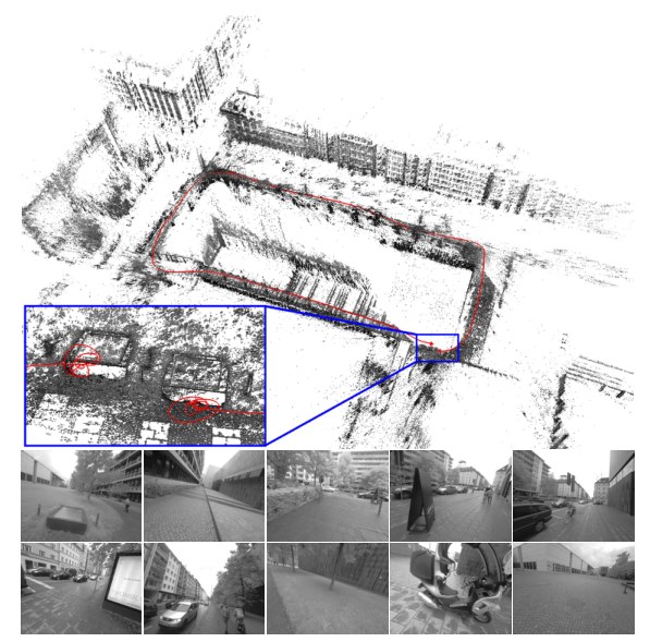
Figure 1. Direct sparse odometry (DSO). 3D reconstruction and tracked trajectory for a 1:40min video cycling around a building (monocular visual odometry only). The bottom-left inset shows a close-up of the start and end point, visualizing the drift accumulated over the course of the trajectory. The bottom row shows some video frames.
图 1:直接稀疏里程计(DSO)。一段环绕建筑物骑行、时长 1 分 40 秒的视频上的三维重建与跟踪轨迹(仅单目视觉里程计)。左下角的插图是起点与终点的放大,用来显示整段轨迹上累积的漂移。底下一行是若干视频帧。
Direct vs. Indirect.
Underlying all formulations is a probabilistic model that takes noisy measurements as input and computes an estimator for the unknown, hidden model parameters (3D world model and camera motion). Typically a Maximum Likelihood approach is used, which finds the model parameters that maximize the probability of obtaining the actual measurements, i.e., .
直接法与间接法。
所有这些表述的底层,都是一个以带噪测量 为输入、为未知的隐模型参数(三维世界模型与相机运动)计算估计量 的概率模型。通常采用最大似然:寻找使获得实际测量的概率最大的模型参数,即 。
Indirect methods then proceed in two steps. First, the raw sensor measurements are pre-processed to generate an intermediate representation, solving part of the overall problem, such as establishing correspondences. Second, the computed intermediate values are interpreted as noisy measurements in a probabilistic model to estimate geometry and camera motion. Note that the first step is typically approached by extracting and matching a sparse set of keypoints – however other options exist, like establishing correspondences in the form of dense, regularized optical flow. It can also include methods that extract and match parametric representations of other geometric primitives, such as line- or curve-segments.
间接方法分两步进行。首先,对原始传感器测量做预处理,生成一种中间表示,从而先解决整体问题的一部分,例如建立对应。其次,把算得的中间量当作概率模型里的带噪测量 ,用来估计几何和相机运动。第一步通常是提取并匹配一组稀疏关键点——不过也有别的做法,例如用稠密、正则化的光流来建立对应。它也可以包括提取并匹配其他几何基元的参数表示,例如线段或曲线段。
Direct methods skip the pre-processing step and directly use the actual sensor values – light received from a certain direction over a certain time period – as measurements in a probabilistic model.
直接方法跳过预处理,直接把实际传感器读数——在某一方向、某一时间段内接收到的光——当作概率模型中的测量 。
In the case of passive vision, the direct approach thus optimizes a photometric error, since the sensor provides photometric measurements. Indirect methods on the other hand optimize a geometric error, since the pre-computed values – point-positions or flow-vecors – are geometric quantities. Note that for other sensor modalities like depth cameras or laser scanners (which directly measure geometric quantities) direct formulations may also optimize a geometric error.
对被动视觉而言,直接法因此优化的是光度误差,因为传感器提供的是光度测量。间接法则优化几何误差,因为预先算出的量——点的位置或流动向量——是几何量。需要注意,对深度相机或激光扫描仪这类直接测量几何量的传感器,直接法表述也可以优化几何误差。
Dense vs. Sparse.
Sparse methods use and reconstruct only a selected set of independent points (traditionally corners), whereas dense methods attempt to use and reconstruct all pixels in the 2D image domain. Intermediate approaches (semi-dense) refrain from reconstructing the complete surface, but still aim at using and reconstructing a (largely connected and well-constrained) subset.
稠密与稀疏。
稀疏方法只使用并重建一组选定的独立点(传统上是角点);稠密方法则试图使用并重建二维图像域中的全部像素。中间做法(半稠密)并不重建完整表面,但仍希望使用并重建一个(大体连通、约束良好的)子集。
Apart from the extent of the used image region however, a more fundamental -- and consequential -- difference lies in the addition of a geometry prior. In the sparse formulation, there is no notion of neighborhood, and geometry parameters (keypoint positions) are conditionally independent given the camera poses & intrinsics[^1]. Dense (or semi-dense) approaches on the other hand exploit the connectedness of the used image region to formulate a geometry prior, typically favouring smoothness. In fact, such a prior is necessarily required to make a dense world model observable from passive vision alone. In general, this prior is formulated directly in the form of an additional log-likelihood energy term [26, 21, 22].
[^1]: Note that even though early filtering-based methods [12, 4] kept track of point-point-correlations, these originated from marginalized camera poses, not from the model itself.
不过,除了所用图像区域的范围之外,一个更根本——也更有后果——的差别在于是否加入几何先验。在稀疏表述里没有邻域的概念,给定相机位姿和内参后,几何参数(关键点位置)是条件独立的[^1]。稠密(或半稠密)方法则利用所用图像区域的连通性来写出几何先验,通常偏好平滑。事实上,若只靠被动视觉,要使稠密的世界模型可观测,这样的先验是必要的。一般而言,先验直接写成额外的对数似然能量项 [26, 21, 22]。
[^1]: 需要说明的是,尽管早期基于滤波的方法 [12, 4] 也会跟踪点与点之间的相关,这些相关来自被边缘化的相机位姿,而不是来自模型本身。
Note that the distinction between dense and sparse is not synonymous to direct and indirect – in fact, all four combinations exist:
需要注意,稠密与稀疏的区分并不等同于直接与间接——事实上,四种组合都存在:
- • Sparse + Indirect: This is the most widely-used formulation, estimating 3D geometry from a set of keypoint-matches, thereby using a geometric error without a geometry prior. Examples include the work of Jin et al. [12], monoSLAM [4], PTAM [16], and ORB-SLAM [20].
- 稀疏 + 间接: 这是使用最广的表述,从一组关键点匹配估计三维几何,因而使用几何误差、不加几何先验。例子包括 Jin 等人的工作 [12]、monoSLAM [4]、PTAM [16] 以及 ORB-SLAM [20]。
- • Dense + Indirect: This formulation estimates 3D geometry from – or in conjunction with – a dense, regularized optical flow field, thereby combining a geometric error (deviation from the flow field) with a geometry prior (smoothness of the flow field), examples include [27, 23].
- 稠密 + 间接: 这种表述从稠密、正则化的光流场估计三维几何,或与之联合估计,从而把几何误差(相对光流场的偏差)与几何先验(光流场的平滑性)结合起来,例子包括 [27, 23]。
- • Dense + Direct: This formulation employs a photometric error as well as a geometric prior to estimate dense or semi-dense geometry. Examples include DTAM [21], its precursor [26], and LSD-SLAM [5].
- 稠密 + 直接: 这种表述同时使用光度误差和几何先验,以估计稠密或半稠密几何。例子包括 DTAM [21]、其前身 [26],以及 LSD-SLAM [5]。
- • Sparse + Direct: This is the formulation proposed in this paper. It optimizes a photometric error defined directly on the images, without incorporating a geometric prior. While we are not aware of any recent work using this formulation, a sparse and direct formulation was already proposed by Jin et al. in 2003 [13]. In contrast to their work however, which is based on an extended Kalman filter, our method uses a non-linear optimization framework. The motivation for exploring the combination of sparse and direct is laid out in the following section.
- 稀疏 + 直接: 这就是本文提出的表述。它直接在图像上优化光度误差,不引入几何先验。我们不知道近年还有哪项工作采用这种表述,不过 Jin 等人在 2003 年已经提出过稀疏直接法 [13]。与他们基于扩展卡尔曼滤波的工作不同,我们的方法使用非线性优化框架。探索稀疏与直接这一组合的动机,将在下一节说明。
1.1 Motivation
1.1 动机
The direct and sparse formulation for monocular visual odometry proposed in this paper is motivated by the following considerations.
本文提出的单目视觉里程计的直接且稀疏表述,出于以下考虑。
(1) Direct: One of the main benefits of keypoints is their ability to provide robustness to photometric and geometric distortions present in images taken with off-the-shelf commodity cameras. Examples are automatic exposure changes, non-linear response functions (gamma correction / white-balancing), lens attenuation (vignetting), de-bayering artefacts, or even strong geometric distortions caused by a rolling shutter.
(1)直接: 关键点的一个主要好处,是能对消费级现成相机所拍图像里的光度和几何畸变保持鲁棒。例如自动曝光变化、非线性响应函数(伽马校正 / 白平衡)、镜头衰减(暗角)、去马赛克伪影,乃至卷帘快门造成的强烈几何畸变。
At the same time, for all use-cases mentioned in the introduction, millions of devices will be (and already are) equipped with cameras solely meant to provide data for computer vision algorithms, instead of capturing images for human consumption. These cameras should and will be designed to provide a complete sensor model, and to capture data in a way that best serves the processing algorithms: Auto-exposure and gamma correction for instance are not unknown noise sources, but features that provide better image data – and that can be incorporated into the model, making the obtained data more informative. Since the direct approach models the full image formation process down to pixel intensities, it greatly benefits from a more precise sensor model.
与此同时,对引言中提到的全部应用而言,将有(并且已经有)数以百万计的设备配备相机,这些相机的目的只是为计算机视觉算法提供数据,而不是给人看的图像。它们应当、也将会被设计成提供完整的传感器模型,并以最有利于处理算法的方式采集数据:例如自动曝光和伽马校正并不是未知噪声源,而是能提供更好图像数据的功能——并且可以被写进模型,使获得的数据更有信息量。由于直接法把成像过程一直建模到像素强度,它会从更精确的传感器模型中显著受益。
One of the main benefits of a direct formulation is that it does not require a point to be recognizable by itself, thereby allowing for a more finely grained geometry representation (pixelwise inverse depth). Furthermore, we can sample from across all available data – including edges and weak intensity variations – generating a more complete model and lending more robustness in sparsely textured environments.
直接法表述的一个主要好处是,它并不要求一个点本身可被识别,从而允许更细粒度的几何表示(逐像素逆深度)。此外,我们可以从所有可用数据中取样——包括边缘和微弱的强度变化——得到更完整的模型,并在纹理稀疏的环境里带来更高的鲁棒性。
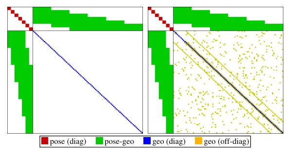
Figure 2. Sparse vs. dense Hessian structure. Left: Hessian structure of sparse bundle adjustment: since the geometry-geometry block is diagonal, it can be solved efficiently using the Schur complement. Right: A geometry prior adds (partially unstructured) geometry-geometry correlations – the resulting system is hence not only much larger, but also becomes much harder to solve. For simplicity, we do not show the global camera intrinsic parameters.
图 2:稀疏与稠密海塞结构。左:稀疏束调整的海塞结构:几何–几何块是对角的,因而可以用舒尔补高效求解。右:加入几何先验后,会增加(部分无结构的)几何–几何相关——系统因此不仅规模大得多,也更难求解。为简单起见,图中未画出全局相机内参。
(2) Sparse: The main drawback of adding a geometry prior is the introduction of correlations between geometry parameters, which render a statistically consistent, joint optimization in real time infeasible (see Figure 2). This is why existing dense or semi-dense approaches (a) neglect or coarsely approximate correlations between geometry parameters (orange), and / or between geometry parameters and camera poses (green), and (b) employ different optimization methods for the dense geometry part, such as a primal-dual formulation [26, 21, 22].
(2)稀疏: 加入几何先验的主要缺点,是在几何参数之间引入相关,使得统计上一致的联合优化无法实时完成(见图 2)。这就是已有稠密或半稠密方法(a)忽略或粗近几何参数之间(橙色),以及/或几何参数与相机位姿之间(绿色)的相关,并且(b)对稠密几何部分改用另一套优化方法,例如原–对偶表述 [26, 21, 22] 的原因。
In addition, the expressive complexity of today’s priors is limited: While they make the 3D reconstruction denser, locally more accurate and more visually appealing, we found that priors can introduce a bias, and thereby reduce rather than increase long-term, large-scale accuracy. Note that in time this may well change with the introduction of more realistic, unbiased priors learnt from real-world data.
此外,今天这些先验的表达能力也有限:虽然它们让三维重建更密、局部更准、看起来更顺眼,我们发现先验可能引入偏差,从而不是提高、反而降低长期、大尺度精度。需要说明的是,随着从真实数据中学习到更真实、无偏的先验,这一点将来完全可能改变。
1.2 Contribution and Outline
1.2 贡献与结构
In this paper we propose a sparse and direct approach to monocular visual odometry. To our knowledge, it is the only fully direct method that jointly optimizes the full likelihood for all involved model parameters, including camera poses, camera intrinsics, and geometry parameters (inverse depth values). This is in contrast to hybrid approaches such as SVO [9], which revert to an indirect formulation for joint model optimization.
本文提出一种稀疏且直接的单目视觉里程计方法。据我们所知,它是唯一对全部相关模型参数——包括相机位姿、相机内参和几何参数(逆深度)——联合优化完整似然的完全直接法。这与 SVO [9] 这类混合方法不同,后者在联合模型优化时会回到间接表述。
Optimization is performed in a sliding window, where old camera poses as well as points that leave the field of view of the camera are marginalized, in a manner inspired by [17]. In contrast to existing approaches, our method further takes full advantage of photometric camera calibration, including lens attenuation, gamma correction, and known exposure times. This integrated photometric calibration further increases accuracy and robustness.
优化在滑动窗口中进行,旧的相机位姿以及离开相机视野的点会被边缘化,做法受到 [17] 的启发。与已有方法不同,我们的方法还充分利用光度相机标定,包括镜头衰减、伽马校正和已知曝光时间。这种集成的光度标定进一步提高了精度和鲁棒性。
Our CPU-based implementation runs in real time on a laptop computer. We show in extensive evaluations on three different datasets comprising several hours of video that it outperforms other state-of-the-art approaches (direct and indirect), both in terms of robustness and accuracy. With reduced settings (less points and active keyframes), it even runs at real-time speed while still outperforming state-of-the-art indirect methods. On high, non-real-time settings in turn (more points and active keyframes), it creates semi-dense models similar in density to those of LSD-SLAM, but much more accurate.
我们基于 CPU 的实现可以在笔记本电脑上实时运行。在三个不同数据集、共计数小时视频上的大量评测表明,无论鲁棒性还是精度,它都优于其他最先进的方法(直接法与间接法)。在降低设置(更少的点和活跃关键帧)时,它甚至能以 实时速度运行,并且仍然优于最先进的间接法。反过来,在更高的非实时设置下(更多的点和活跃关键帧),它能生成密度与 LSD-SLAM 相近、但准确得多的半稠密模型。
The paper is organized as follows: The proposed direct, sparse model as well as the windowed optimization method are described in Section 2. Specifically, this comprises the geometric and photometric camera calibration in Section 2.1, the model formulation in Section 2.2, and the windowed optimization in Section 2.3. Section 3 describes the front-end: the part of the algorithm that performs data-selection and provides sufficiently accurate initializations for the highly non-convex optimization back-end. We provide a thorough experimental comparison to other methods in Section 4.1. We also evaluate the effect of important parameters and new concepts like the use of photometric calibration in Section 4.2. In Section 4.3, we analyse the effect of added photometric and geometric noise to the data. Finally, we provide a summary in Section 5.
论文组织如下:第 2 节描述所提出的直接稀疏模型以及窗口优化方法。具体而言,第 2.1 节是几何与光度相机标定,第 2.2 节是模型表述,第 2.3 节是窗口优化。第 3 节描述前端:负责选取数据、并为高度非凸的优化后端提供足够准确初值的那一部分算法。第 4.1 节给出与其他方法的充分实验比较。第 4.2 节评测重要参数以及光度标定等新概念的影响。第 4.3 节分析在数据中加入光度和几何噪声后的影响。最后,第 5 节给出总结。
2 Direct Sparse Model
2 直接稀疏模型
Our direct sparse odometry is based on continuous optimization of the photometric error over a window of recent frames, taking into account a photometrically calibrated model for image formation. In contrast to existing direct methods, we jointly optimize for all involved parameters (camera intrinsics, camera extrinsics, and inverse depth values), effectively performing the photometric equivalent of windowed sparse bundle adjustment. We keep the geometry representation employed by other direct approaches, i.e., 3D points are represented as inverse depth in a reference frame (and thus have one degree of freedom).
我们的直接稀疏里程计,是在最近若干帧组成的窗口上连续优化光度误差,并采用经过光度标定的成像模型。与已有直接法不同,我们对全部相关参数(相机内参、外参和逆深度)做联合优化,实际上是在做窗口稀疏束调整的光度对应物。几何表示仍沿用其他直接法:三维点表示成参考帧中的逆深度(因而只有一个自由度)。
Notation.
Throughout the paper, bold lower-case letters () represent vectors and bold upper-case letters () represent matrices. Scalars will be represented by light lower-case letters (), functions (including images) by light upper-case letters (). Camera poses are represented as transformation matrices , transforming a point from the world frame into the camera frame. Linearized pose-increments will be expressed as Lie-algebra elements , which – with a slight abuse of notation – we directly write as vectors . We further define the commonly used operator using a left-multiplicative formulation, i.e.,
记号。
全文用粗体小写字母()表示向量,粗体大写字母()表示矩阵。标量用细体小写字母(),函数(包括图像)用细体大写字母()。相机位姿表示成变换矩阵 ,把点从世界坐标系变到相机坐标系。线性化后的位姿增量写成李代数元素 ,并——略微滥用记号——直接写成向量 。我们还用左乘形式定义常用算子 ,即
2.1 Calibration
2.1 标定
The direct approach comprehensively models the image formation process. In addition to a geometric camera model – which comprises the function that projects a 3D point onto the 2D image – it is hence beneficial to also consider a photometric camera model, which comprises the function that maps real-world energy received by a pixel on the sensor (irradiance) to the respective intensity value. Note that for indirect methods this is of little benefit and hence widely ignored, as common feature extractors and descriptors are invariant (or highly robust) to photometric variations.
直接法对成像过程做比较完整的建模。除了几何相机模型——也就是把三维点投影到二维图像上的那个函数——之外,再考虑一个光度相机模型是有益的:它把传感器上某个像素接收到的真实世界能量(辐照度)映射为相应的强度值。对间接法来说,这一点好处不大,因而普遍被忽略,因为常见的特征提取器和描述子对光度变化是不变的(或高度鲁棒的)。
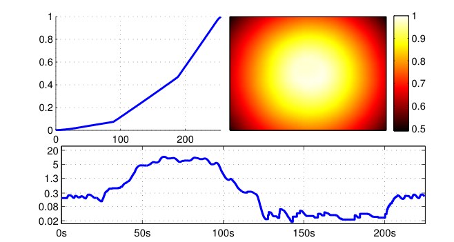
Figure 3. Photometric calibration. Top: Inverse response function and lens attenuation of the camera used for Figure 1. Bottom: Exposure in milliseconds for a sequence containing an indoor and an outdoor part. Note how it varies by a factor of more than 500, from 0.018 to 10.5ms. Instead of treating these quantities as unknown noise sources, we explicitly account for them in the photometric error model.
图 3:光度标定。上:图 1 所用相机的逆响应函数 与镜头衰减 。下:一段同时包含室内与室外部分的序列中,曝光时间 (毫秒)。注意它变化了 500 倍以上,从 0.018 毫秒到 10.5 毫秒。我们不把这些量当成未知噪声,而是在光度误差模型里显式计入。
2.1.1 Geometric Camera Calibration
For simplicity, we formulate our method for the well-known pinhole camera model – radial distortion is removed in a preprocessing step. While for wide-angle cameras this does reduce the field of view, it allows comparison across methods that only implement a limited choice of camera models. Throughout this paper, we will denote projection by and back-projection with , where denotes the intrinsic camera parameters (for the pinhole model these are the focal length and the principal point). Note that analogously to [2], our approach can be extended to other (invertible) camera models, although this does increase computational demands.
2.1.1 几何相机标定
为简单起见,我们按熟知的针孔相机模型来写方法——径向畸变在预处理步骤中去掉。对广角相机而言,这会减小视场,但便于与只实现了有限几种相机模型的方法做比较。全文用 表示投影,用 表示反投影,其中 表示相机内参(对针孔模型而言就是焦距和主点)。与 [2] 类似,我们的方法也可以推广到其他(可逆的)相机模型,不过计算量会增加。
2.1.2 Photometric Camera Calibration
We use the image formation model used in [8], which accounts for a non-linear response function , as well as lens attenuation (vignetting) . Figure 3 shows an example calibration from the TUM monoVO dataset. The combined model is then given by
2.1.2 光度相机标定
我们采用 [8] 中的成像模型,它计入非线性响应函数 ,以及镜头衰减(暗角)。图 3 给出了 TUM monoVO 数据集上的一个标定示例。组合模型为
where and are the irradiance and the observed pixel intensity in frame , and is the exposure time. The model is applied by photometrically correcting each video frame as very first step, by computing
其中 和 分别是第 帧中的辐照度和观测到的像素强度, 是曝光时间。该模型的用法是:作为非常靠前的一步,先对每一视频帧做光度校正,计算
In the remainder of this paper, will always refer to the photometrically corrected image , except where otherwise stated.
在本文余下部分,除另有说明外, 一律指经过光度校正的图像 。
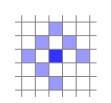
Figure 4. Residual pattern. Pattern used for energy computation. The bottom-right pixel is omitted to enable SSE-optimized processing. Note that since we have 1 unknown per point (its inverse depth), and do not use a regularizer, we require in order for all model parameters to be well-constrained when optimizing over only two frames. Figure 19 shows an evaluation of how this pattern affects tracking accuracy.
图 4:残差图案。用于计算能量的图案 。右下角那个像素被去掉,以便用 SSE 做优化计算。注意每个点只有 1 个未知量(其逆深度),而且我们不用正则项,因此在只对两帧优化时,需要 ,才能把所有模型参数都约束住。图 19 给出了这一图案对跟踪精度的评测。
2.2 Model Formulation
2.2 模型表述
We define the photometric error of a point in reference frame , observed in a target frame , as the weighted SSD over a small neighborhood of pixels. Our experiments have shown that 8 pixels, arranged in a slightly spread pattern (see Figure 4) give a good trade-off between computations required for evaluation, robustness to motion blur, and providing sufficient information. Note that in terms of the contained information, evaluating the SSD over such a small neighborhood of pixels is similar to adding first- and second-order irradiance derivative constancy terms (in addition to irradiance constancy) for the central pixel. Let
我们把参考帧 中一点 在目标帧 中被观测到时的光度误差,定义为在一个小像素邻域上的加权 SSD。实验表明,8 个像素、排成略微散开的图案(见图 4),在计算量、对运动模糊的鲁棒性、以及所含信息量之间是较好的折中。就所含信息而言,在这样的小邻域上计算 SSD,类似于在辐照度恒常之外,再为中心像素加上一阶和二阶辐照度导数恒常项。令
where is the set of pixels included in the SSD; the exposure times of the images ; and the Huber norm. Further, stands for the projected point position of with inverse depth , given by
其中 是计入 SSD 的像素集合; 是图像 的曝光时间; 是 Huber 范数。此外, 表示逆深度为 的点 投影后的位置,由下式给出
with
其中
$$\displaystyle\begin{bmatrix}\mathbf{R}&\mathbf{t}\
0&1\end{bmatrix}:=\mathbf{T}{j}\mathbf{T}{i}^{-1}. \tag{6}$$
In order to allow our method to operate on sequences without known exposure times, we include an additional affine brightness transfer function given by . Note that in contrast to most previous formulations [13, 6], the scalar factor is parametrized logarithmically. This both prevents it from becoming negative, and avoids numerical issues arising from multiplicative (i.e., exponentially increasing) drift.
为了让方法也能用在没有已知曝光时间的序列上,我们额外加入仿射亮度传递函数 。与以往多数表述 [13, 6] 不同,标量因子 采用对数参数化。这既避免它变成负数,也避免乘性(也就是指数增长的)漂移带来的数值问题。
In addition to using robust Huber penalties, we apply a gradient-dependent weighting given by
除了使用稳健的 Huber 惩罚,我们还施加依赖于梯度的权重 ,定义为
which down-weights pixels with high gradient. This weighting function can be probabilistically interpreted as adding small, independent geometric noise on the projected point position , and immediately marginalizing it – approximating small geometric error. To summarize, the error depends on the following variables: (1) the point’s inverse depth , (2) the camera intrinsics , (3) the poses of the involved frames , and (4) their brightness transfer function parameters .
它会下调梯度大的像素的权重。从概率上看,这个加权函数可以理解为:在投影点位置 上加上很小的独立几何噪声,并立刻把它边缘化——相当于近似小的几何误差。总结起来,误差 依赖于下列变量:(1)该点的逆深度 ,(2)相机内参 ,(3)所涉及帧的位姿 ,以及(4)它们的亮度传递函数参数 。
The full photometric error over all frames and points is given by
所有帧和所有点上的完整光度误差为
where runs over all frames , over all points in frame , and over all frames in which the point is visible. Figure 5 shows the resulting factor graph: The only difference to the classical reprojection error is the additional dependency of each residual on the pose of the host frame, i.e., each term depends on two frames instead of only one. While this adds off-diagonal entries to the pose-pose block of the Hessian, it does not affect the sparsity pattern after application of the Schur complement to marginalize point parameters. The resulting system can thus be solved analogously to the indirect formulation. Note that the Jacobians with respect to the two frames’ poses are linearly related by the adjoint of their relative pose. In practice, this factor can then be pulled out of the sum when computing the Hessian or its Schur complement, greatly reducing the additional computations caused by more variable dependencies.
其中 遍历所有帧 , 遍历第 帧中的所有点 , 遍历能看到点 的所有帧 。图 5 给出了由此得到的因子图:与经典重投影误差的唯一差别,是每个残差还额外依赖于宿主帧的位姿,也就是说,每一项依赖于两帧而不是一帧。这会在海塞矩阵的位姿–位姿块中增加非对角项,但在用舒尔补边缘化点参数之后,并不改变稀疏模式。因此,得到的系统可以按与间接表述相同的方式求解。注意,关于两帧位姿的雅可比由它们相对位姿的伴随线性地联系在一起。实践中,计算海塞或其舒尔补时可以把这个因子提到求和号外面,从而大大减少因变量依赖增多而带来的额外计算。
If exposure times are known, we further add a prior pulling the affine brightness transfer function to zero:
若曝光时间已知,我们再加一项先验,把仿射亮度传递函数往零拉:
If no photometric calibration is available, we set and , as in this case they need to model the (unknown) changing exposure time of the camera. As a side-note it should be mentioned that the ML estimator for a multiplicative factor is biased if both and contain noisy measurements (see [7]); causing to drift in the unconstrained case . While this generally has little effect on the estimated poses, it may introduce a bias if the scene contains only few, weak intensity variations.
若没有光度标定,我们令 且 ,因为这时它们需要去建模相机未知的曝光变化。顺便指出,若 和 都含有带噪测量,则乘性因子的最大似然估计 是有偏的(见 [7]);在无约束情形 时,这会导致 漂移。这对估计出的位姿一般影响不大,但如果场景里只有很少、很弱的强度变化,则可能引入偏差。
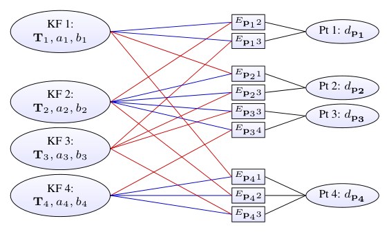
Figure 5. Factor graph for the direct sparse model. Example with four keyframes and four points; one in KF1, two in KF2, and one in KF4. Each energy term (defined in Eq. (4)) depends on the point’s host frame (blue), the frame the point is observed in (red), and the point’s inverse depth (black). Further, all terms depend on the global camera intrinsics vector , which is not shown.
图 5:直接稀疏模型的因子图。示例含四个关键帧和四个点:一个在 KF1,两个在 KF2,一个在 KF4。每个能量项(由式 (4) 定义)依赖于该点的宿主帧(蓝)、观测到该点的帧(红),以及该点的逆深度(黑)。此外,所有项还依赖于未在图中画出的全局相机内参向量 。
Point Dimensionality.
In the proposed direct model, a point is parametrized by only one parameter (the inverse depth in the reference frame), in contrast to three unknowns as in the indirect model. To understand the reason for this difference, we first note that in both cases a 3D point is in fact an arbitrarily located discrete sample on a continuous, real-world 3D surface. The difference then lies in the way this 2D location on the surface is defined. In the indirect approach, it is implicitly defined as the point, which (projected into an image) generates a maximum in the used corner response function. This entails that both the surface, as well as the point’s location on the surface are unknowns, and need to be estimated. In our direct formulation, a point is simply defined as the point, where the source pixel’s ray hits the surface, thus only one unknown remains. In addition to a reduced number of parameters, this naturally enables an inverse depth parametrization, which – in a Gaussian framework – is better suited to represent uncertainty from stereo-based depth estimation, in particular for far-away points [3].
点的维数。
在所提出的直接模型里,一个点只用一个参数来参数化(参考帧中的逆深度),而间接模型有三个未知量。要理解这一差别,首先注意到:两种情形下,三维点其实都是连续真实三维表面上一个位置任意的离散采样。差别在于这个表面上的二维位置如何定义。间接法里,它被隐含地定义为投影到图像中、使所用角点响应函数取极大的那个点。这意味着表面本身,以及点在表面上的位置,都是未知量,都需要估计。在我们的直接表述里,一个点就定义为源像素射线与表面相交的那个点,因而只剩一个未知量。除了参数更少,这还自然地允许采用逆深度参数化——在高斯框架下,它更适合表示基于立体的深度估计的不确定性,对远处的点尤其如此 [3]。
Consistency.
Strictly speaking, the proposed direct sparse model does allow to use some observations (pixel values) multiple times, while others are not used at all. This is because – even though our point selection strategy attempts to avoid this by equally distributing points in space (see Section 3.2) – we allow point observations to overlap, and thus depend on the same pixel value(s). This particularly happens in scenes with little texture, where all points have to be chosen from a small subset of textured image regions. We however argue that this has negligible effect in practice, and – if desired – can be avoided by removing (or downweighting) observations that use the same pixel value.
一致性。
严格来说,所提出的直接稀疏模型允许某些观测(像素值)被使用多次,而另一些则完全没用到。这是因为——尽管我们的选点策略试图通过在空间中均匀分布点来避免这一点(见第 3.2 节)——我们允许点的观测发生重叠,从而依赖于同一个(或同一些)像素值。在纹理很少的场景里尤其如此,那时所有点都不得不从一小块有纹理的图像区域里选取。不过我们认为这在实践中影响可以忽略;如果希望避免,也可以去掉(或下调)使用了同一像素值的观测。
2.3 Windowed Optimization
2.3 窗口优化
We follow the approach by Leutenegger et al. [17] and optimize the total error (8) in a sliding window using the Gauss-Newton algorithm, which gives a good trade-off between speed and flexibility.
我们沿用 Leutenegger 等人 [17] 的做法,用高斯–牛顿算法在滑动窗口里优化总误差 (8),以求在速度和灵活性之间取得较好折中。
For ease of notation, we extend the operator as defined in (1) to all optimized parameters – for parameters other than SE(3) poses it denotes conventional addition. We will use to denote all optimized variables, including camera poses, affine brightness parameters, inverse depth values, and camera intrinsics. As in [17], marginalizing a residual that depends on a parameter in will fix the tangent space in which any future information (delta-updates) on that parameter is accumulated. We will denote the evaluation point for this tangent space with , and the accumulated delta-updates by . The current state estimate is hence given by . Figure 6 visualizes the relation between the different variables.
为便于书写,我们把 (1) 中定义的 算子推广到全部优化参数——对 SE(3) 位姿以外的参数,它就是普通加法。我们用 表示全部优化变量,包括相机位姿、仿射亮度参数、逆深度和相机内参。与 [17] 一样,一旦边缘化一个依赖于 中某参数的残差,就会固定该参数此后累积信息(增量更新)所在的切空间。我们把这个切空间的求值点记为 ,把累积的增量更新记为 。当前状态估计因而由 给出。图 6 画出了这些变量之间的关系。
Gauss-Newton Optimization.
We compute the Gauss-Newton system as
高斯–牛顿优化。
我们把高斯–牛顿系统写成
where is the diagonal matrix containing the weights, is the stacked residual vector, and is the Jacobian of .
其中 是含权重的对角矩阵, 是堆叠后的残差向量, 是 的雅可比。
Note that each point contributes residuals to the energy. For notational simplicity, we will in the following consider only a single residual , and the associated row of the Jacobian . During optimization – as well as when marginalizing – residuals are always evaluated at the current state estimate, i.e.,
注意每个点为能量贡献 个残差。为书写简便,下面只考虑单个残差 以及相应的雅可比行 。在优化——以及边缘化——时,残差总是在当前状态估计处求值,即
where are the current state variables the residual depends on. The Jacobian is evaluated with respect to an additive increment to , i.e.,
其中 是该残差所依赖的当前状态变量。雅可比 是关于 的加性增量求值的,即
It can be decomposed as
它可以分解为
where denotes the “geometric” parameters , and denotes the “photometric” parameters . We employ two approximations, described below.
其中 表示“几何”参数 , 表示“光度”参数 。我们采用下面所述的两个近似。
First, both and are evaluated at . This technique is called “First Estimate Jacobians” [17, 11], and is required to maintain consistency of the system and prevent the accumulation of spurious information. In particular, in the presence of non-linear null-spaces in the energy (in our formulation absolute pose and scale), adding linearizations around different evaluation points eliminates these and thus slowly corrupts the system. In practice, this approximation is very good, since , are smooth compared to the size of the increment . In contrast, is much less smooth, but does not affect the null-spaces. Thus, it is evaluated at the current value for , i.e., at the same point as the residual . We use centred differences to compute the image derivatives at integer positions, which are then bilinearly interpolated.
第一, 和 都在 处求值。这一技术称为“首次估计雅可比”(First Estimate Jacobians)[17, 11],是为了保持系统一致性、防止虚假信息累积。特别是,当能量中存在非线性零空间时(在我们的表述里是绝对位姿和尺度),如果在不同求值点附近做线性化再相加,就会消除这些零空间,从而缓慢腐蚀系统。实践中这一近似很好,因为相对于增量 的大小,、 是光滑的。相比之下, 远没有那么光滑,但不影响零空间。因此,它在 的当前值处求值,也就是与残差 相同的点。图像导数在整数位置用中心差分计算,再双线性插值。
Second, is assumed to be the same for all residuals belonging to the same point, and evaluated only for the center pixel. Again, this approximation is very good in practice. While it significantly reduces the required computations, we have not observed a notable effect on accuracy for any of the used datasets.
第二,假定属于同一点的所有残差共用同一个 ,并且只对中心像素求值。这一近似在实践中同样很好。它显著减少了所需计算,而我们在所用的任何数据集上都没有观察到对精度有明显影响。
From the resulting linear system, an increment is computed as and added to the current state:
由得到的线性系统,增量按 计算,并加到当前状态上:
Note that due to the First Estimate Jacobian approximation, a multiplicative formulation (replacing with in (12)) results in the exact same Jacobian, thus a multiplicative update step is equally valid.
注意,由于采用了首次估计雅可比近似,乘性表述(把 (12) 中的 换成 )会得到完全相同的雅可比,因此乘性更新步 同样成立。
After each update step, we update for all variables that are not part of the marginalization term, using and . In practice, this includes all depth values, as well as the pose of the newest keyframe. Each time a new keyframe is added, we perform up to 6 Gauss-Newton iterations, breaking early if is sufficiently small. We found that – since we never start far-away from the minimum – a Levenberg-Marquad dampening (which slows down convergence) is not required.
每做完一步更新,我们用 以及 ,对所有尚未进入边缘化项的变量更新 。实践中,这包括全部深度值,以及最新关键帧的位姿。每加入一个新关键帧,我们最多做 6 次高斯–牛顿迭代,若 已足够小就提前停止。我们发现——因为从未从离极小值很远的地方起步——并不需要会减慢收敛的 Levenberg–Marquardt 阻尼。
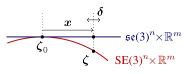
Figure 6. Windowed optimization. The red curve denotes the parameter space, composed of non-Euclidean camera poses in , and the remaining Euclidean parameters. The blue line corresponds to the tangent-space around , in which we (1) accumulate the quadratic marginalization-prior on , and (2) compute Gauss-Newton steps . For each parameter, the tangent space is fixed as soon as that parameter becomes part of the marginalization term. Note that while we treat all parameters equally in our notation, for Euclidean parameters tangent-space and parameter-space coincide.
图 6:窗口优化。红线表示参数空间,由 中的非欧相机位姿以及其余欧氏参数组成。蓝线是 附近的切空间,我们在其中(1)累积关于 的二次边缘化先验,(2)计算高斯–牛顿步 。对每个参数,一旦它进入边缘化项,切空间就被固定下来。虽然记号上我们对所有参数一视同仁,但对欧氏参数而言,切空间与参数空间是重合的。
Marginalization.
When the active set of variables becomes too large, old variables are removed by marginalization using the Schur complement. Similar to [17], we drop any residual terms that would affect the sparsity pattern of : When marginalizing frame , we first marginalize all points in , as well as points that have not been observed in the last two keyframes. Remaining observations of active points in frame are dropped from the system.
边缘化。
当活跃变量集合变得太大时,用舒尔补把旧变量边缘化掉。与 [17] 类似,我们丢掉任何会破坏 稀疏模式的残差项:在边缘化第 帧时,先边缘化 中的所有点,以及在最近两个关键帧中未被观测到的点。活跃点在第 帧中的其余观测则从系统中丢掉。
Marginalization proceeds as follows: Let denote the part of the energy containing all residuals that depend on state variables to be marginalized. We first compute a Gauss-Newton approximation of around the current state estimate . This gives
边缘化步骤如下:令 表示能量中、所有依赖于待边缘化状态变量的残差所构成的那一部分。我们先在当前状态估计 附近计算 的高斯–牛顿近似。这给出
where denotes the current value (evaluation point for ) of . The constants can be dropped, and are defined as in (10-13). This is a quadratic function on , and we can apply the Schur complement to marginalize a subset of variables. Written as a linear system, it becomes
其中 表示 的当前值( 的求值点)。常数 可以丢掉, 按 (10-13) 定义。这是关于 的二次函数,我们可以用舒尔补边缘化其中一部分变量。写成线性系统,即为
$$\displaystyle\begin{bmatrix}\mathbf{H}{\alpha\alpha}&\mathbf{H}{\alpha\beta}\
\mathbf{H}{\beta\alpha}&\mathbf{H}{\beta\beta}\end{bmatrix}\begin{bmatrix}{{\boldsymbol{x}}}{\alpha}\
{{\boldsymbol{x}}}{\beta}\end{bmatrix}=\begin{bmatrix}\mathbf{b}^{\prime}{\alpha}\
\mathbf{b}^{\prime}{\beta}\end{bmatrix}, \tag{16}$$
where denotes the block of variables we would like to marginalize, and the block of variables we would like to keep. Applying the Schur complement yields , with
其中 表示我们希望边缘化的那一块变量, 表示希望保留的那一块。做舒尔补得到 ,其中
The residual energy on can hence be written as
因此, 上的残差能量可以写成
This is a quadratic function on and can be trivially added to the full photometric error during all subsequent optimization and marginalization operations, replacing the corresponding non-linear terms. Note that this requires the tangent space for to remain the same for all variables that appear in during all subsequent optimization and marginalization steps.
这是关于 的二次函数,可以在随后所有优化和边缘化步骤中直接加到完整光度误差 上,以替换相应的非线性项。注意,这要求在随后所有优化和边缘化步骤中,出现在 里的所有变量,其 的切空间保持不变。
3 Visual Odometry Front-End
3 视觉里程计前端
The front end is the part of the algorithm that
前端是算法中负责以下事项的部分
- • determines the sets , and that make up the error terms of . It decides which points and frames are used, and in which frames a point is visible – in particular, this includes outlier removal and occlusion detection.
- 确定构成 误差项的集合 、 以及 。它决定使用哪些点和哪些帧,以及一个点在哪些帧中可见——这其中特别包括去除外点和遮挡检测。
- • provides initializations for new parameters, required for optimizing the highly non-convex energy function . As a rule of thumb, a linearization of the image is only valid in a 1-2 pixel radius; hence all parameters involved in computing should be initialized sufficiently accurately for to be off by no more than 1-2 pixels.
- 为新参数提供初值,这是优化高度非凸的能量函数 所需要的。经验上,图像 的线性化只在 1–2 个像素的半径内有效;因此,所有参与计算 的参数都应当初始化得足够准,使 的偏差不超过 1–2 个像素。
- • decides when a point / frame should be marginalized.
- 决定何时应当把一个点 / 一帧边缘化。
As such, the front-end needs to replace many operations that in the indirect setting are accomplished by keyframe detectors (determining visibility, point selection) and initialization procedures such as RANSAC. Note that many procedures described here are specific to the monocular case. For instance, using a stereo camera makes obtaining initial depth values more straightforward, while integration of an IMU can significantly robustify – or even directly provide – a pose initialization for new frames.
因此,前端需要替代间接法设定里由关键帧检测器(判断可见性、选点)以及 RANSAC 这类初始化程序完成的许多操作。注意,这里描述的许多步骤是单目情形所特有的。例如,使用双目相机后,获得初始深度会更直接;而接入 IMU 可以显著增强——甚至直接提供——新帧的位姿初值。
3.1 Frame Management
3.1 帧管理
Our method always keeps a window of up to active keyframes (we use ). Every new frame is initially tracked with respect to these reference frames (Step 1). It is then either discarded or used to create a new keyframe (Step 2). Once a new keyframe – and respective new points – are created, the total photometric error (8) is optimized. Afterwards, we marginalize one or more frames (Step 3).
我们的方法始终保持一个最多 个活跃关键帧的窗口(我们取 )。每一新帧先相对这些参考帧做初始跟踪(步骤 1)。然后它要么被丢掉,要么用来生成新的关键帧(步骤 2)。一旦新的关键帧以及相应的新点被创建,就优化总光度误差 (8)。随后,我们边缘化一帧或多帧(步骤 3)。
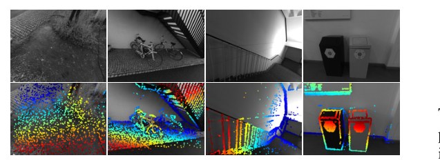
Figure 7. Example depth maps used for initial frame tracking. The top row shows the original images, the bottom row the color-coded depth maps. Since we aim at a fixed number of points in the active optimization, they become more sparse in densely textured scenes (left), while becoming similar in density to those of LSD-SLAM in scenes where only few informative image regions are available to sample from (right).
图 7:用于初始帧跟踪的深度图示例。上一行是原始图像,下一行是伪彩色深度图。因为我们希望活跃优化里的点数固定,在纹理密集的场景里(左)这些点会更稀;而在只能从很少几块有信息的图像区域取样的场景里(右),密度会接近 LSD-SLAM。
Step 1: Initial Frame Tracking.
When a new keyframe is created, all active points are projected into it and slightly dilated, creating a semi-dense depth map. New frames are tracked with respect to only this frame using conventional two-frame direct image alignment, a multi-scale image pyramid and a constant motion model to initialize. Figure 7 shows some examples – we found that further increasing the density has little to no benefit in terms of accuracy or robustness, while significantly increasing runtime. Note that when down-scaling the images, a pixel is assigned a depth value if at least one of the source pixels has a depth value as in [24], significantly increasing the density on coarser resolutions.
步骤 1:初始帧跟踪。
当创建一个新关键帧时,所有活跃点被投影到该帧上并略做膨胀,生成半稠密深度图。新帧只相对这一帧、用常规的两帧直接图像对齐来跟踪,采用多尺度图像金字塔,并用匀速运动模型做初始化。图 7 给出了一些例子——我们发现再提高密度对精度或鲁棒性几乎没有好处,却会显著增加运行时间。注意,在对图像降采样时,只要源像素中至少有一个有深度值,该像素就被赋予深度,做法同 [24],从而在更粗的分辨率上显著提高密度。
If the final RMSE for a frame is more than twice that of the frame before, we assume that direct image alignment failed and attempt to recover by initializing with up to 27 different small rotations in different directions. This recovery-tracking is done on the coarsest pyramid level only, and takes approximately 0.5ms per try. Note that this RANSAC-like procedure is only rarely invoked, such as when the camera moves very quickly shakily. Tightly integrating an IMU would likely render this unnecessary.
如果某一帧最终的 RMSE 超过前一帧的两倍,我们就认为直接图像对齐失败了,并尝试用最多 27 个不同方向上的小旋转来初始化,以求恢复。这种恢复性跟踪只在最粗的金字塔层上进行,每次大约耗时 0.5 毫秒。注意,这种类似 RANSAC 的步骤很少被调用,例如只在相机快速、抖动地运动时。若紧密接入 IMU,很可能就不再需要它。
Step 2: Keyframe Creation.
Similar to ORB-SLAM, our strategy is to initially take many keyframes (around 5-10 keyframes per second), and sparsify them afterwards by early marginalizing redundant keyframes. We combine three criteria to determine if a new keyframe is required:
步骤 2:关键帧创建。
与 ORB-SLAM 类似,我们的策略是一开始多取关键帧(大约每秒 5–10 个),再通过尽早边缘化冗余关键帧把它们稀疏化。我们结合三个准则来判断是否需要新的关键帧:
- New keyframes need to be created as the field of view changes. We measure this by the mean square optical flow (from the last keyframe to the latest frame) during initial coarse tracking.
- 视场变化时需要创建新关键帧。我们用初始粗跟踪期间(从上一关键帧到最新帧)的均方光流 来度量这一点。
- Camera translation causes occlusions and dis-occlusions, which requires more keyframes to be taken (even though may be small). This is measured by the mean flow without rotation, i.e., , where is the warped point position with .
- 相机平移会造成遮挡与去遮挡,因而需要取更多关键帧(即使 可能很小)。这用不含旋转的平均流动来度量,即 ,其中 是取 时变形后的点位置。
- If the camera exposure time changes significantly, a new keyframe should be taken. This is measured by the relative brightness factor between two frames .
- 若相机曝光时间变化显著,应当取新的关键帧。这用两帧之间的相对亮度因子 来度量。
These three quantities can be obtained easily as a by-product of initial alignment. Finally, a new keyframe is taken if , where provide a relative weighting of these three indicators, and by default.
这三个量都可以作为初始对齐的副产品很容易得到。最后,若 ,就取一个新关键帧,其中 给出这三项指标的相对权重,默认 。
Step 3: Keyframe Marginalization.
Our marginalization strategy is as follows (let be the set of active keyframes, with being the newest and being the oldest):
步骤 3:关键帧边缘化。
我们的边缘化策略如下(令 为活跃关键帧集合, 最新, 最旧):
- We always keep the latest two keyframes ( and ).
- 始终保留最近的两个关键帧( 和 )。
- Frames with less than 5% of their points visible in are marginalized.
- 在 中可见点数不足 5% 的帧被边缘化。
- If more than frames are active, we marginalize the one (excluding and ) which maximizes a “distance score” , computed as (20) where is the Euclidean distance between keyframes and , and a small constant. This scoring function is heuristically designed to keep active keyframes well-distributed in 3D space, with more keyframes close to the most recent one.
- 若活跃帧数超过 ,我们就边缘化(除 和 以外)使“距离分数” 最大的那一帧,其计算为 (20) 其中 是关键帧 与 之间的欧氏距离, 是一个小常数。这一评分函数是启发式设计的,目的是让活跃关键帧在三维空间中分布良好,并且在最新一帧附近布置更多关键帧。
A keyframe is marginalized by first marginalizing all points represented in it, and then the frame itself, using the marginalization procedure from Section 2.3. To preserve the sparsity structure of the Hessian, all observations of still existing points in the frame are dropped from the system. While this is clearly suboptimal (in practice about half of all residuals are dropped for this reason), it allows to efficiently optimize the energy function. Figure 8 shows an example of a scene, highlighting the active set of points and frames.
边缘化一个关键帧时,先边缘化其中表示的所有点,再边缘化该帧本身,采用第 2.3 节的边缘化步骤。为保持海塞矩阵的稀疏结构,该帧中仍然存在的点的全部观测都会从系统中丢掉。这显然并非最优(实践中约一半残差因此被丢掉),却使能量函数可以高效优化。图 8 给出了一个场景示例,标出了活跃的点和帧。
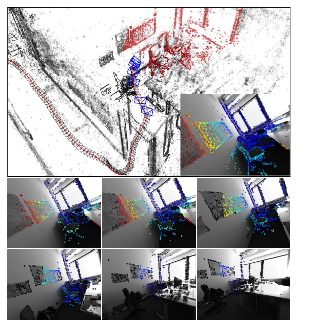
Figure 8. Keyframe management. Bottom rows: The 6 old keyframes in the optimization window, overlaid with the points hosted in them (already marginalized points are shown in black). The top image shows the full point cloud, as well as the positions of all keyframes (black camera frustums) – active points and keyframes are shown in red and blue respectively. The inlay shows the newly added keyframe, overlaid with all forward-warped active points, which will be used for initial alignment of subsequent frames.
图 8:关键帧管理。下面几行:优化窗口里的 6 个旧关键帧,并叠上寄宿在这些帧里的点(已经边缘化的点画成黑色)。上图是完整点云以及所有关键帧的位置(黑色相机椎体)——活跃点和活跃关键帧分别用红、蓝表示。插图是新加入的关键帧,叠上所有前向变形后的活跃点,后续帧的初始对齐会用到它们。
3.2 Point Management
3.2 点管理
Most existing direct methods focus on utilizing as much image data as possible. To achieve this in real time, they accumulate early, sub-optimal estimates (linearizations / depth triangulations), and ignore – or approximate – correlations between different parameters. In this work, we follow a different approach, and instead heavily sub-sample data to allow processing it in real time in a joint optimization framework. In fact, our experiments show that image data is highly redundant, and the benefit of simply using more data points quickly flattens off. Note that in contrast to indirect methods, our direct framework still allows to sample from across all available data, including weakly textured or repetitive regions and edges, which does provide a real benefit (see Section 4).
已有的多数直接法着眼于尽可能利用更多图像数据。为了实时做到这一点,它们会累积早期、并不最优的估计(线性化 / 深度三角化),并忽略——或近似——不同参数之间的相关。本文采取不同做法:对数据做大幅子采样,以便在联合优化框架里实时处理。事实上,我们的实验表明图像数据高度冗余,仅仅使用更多数据点的收益很快就会变平。需要注意,与间接法不同,我们的直接法框架仍然允许从所有可用数据中取样,包括弱纹理或重复区域以及边缘,而这确实带来实际好处(见第 4 节)。
We aim at always keeping a fixed number of active points (we use ), equally distributed across space and active frames, in the optimization. In a first step, we identify candidate points in each new keyframe (Step 1). Candidate points are not immediately added into the optimization, but instead are tracked individually in subsequent frames, generating a coarse depth value which will serve as initialization (Step 2). When new points need to be added to the optimization, we choose a number of candidate points (from across all frames in the optimization window) to be activated, i.e., added into the optimization (Step 3). Note that we choose candidates in each frame, however only keep active points across all active frames combined. This assures that we always have sufficient candidates to activate, even though some may become invalid as they leave the field of view or are identified as outliers.
我们希望在优化中始终保持固定数目 的活跃点(我们取 ),并在空间和活跃帧之间均匀分布。第一步,在每个新关键帧中识别 个候选点(步骤 1)。候选点并不立即加入优化,而是在后续帧中被单独跟踪,生成一个粗深度,作为初始化(步骤 2)。当需要向优化中加入新点时,我们从优化窗口里的所有帧中选取若干候选点加以激活,也就是加入优化(步骤 3)。注意,我们在每一帧选取 个候选,但只在全部活跃帧合计时保持 个活跃点。这样可以保证始终有足够的候选可供激活,即使有些会因离开视野或被判为外点而失效。
Step 1: Candidate Point Selection.
Our point selection strategy aims at selecting points that are (1) well-distributed in the image and (2) have sufficiently high image gradient magnitude with respect to their immediate surroundings. We obtain a region-adaptive gradient threshold by splitting the image into blocks. For each block, we then compute the threshold as , where is the median absolute gradient over all pixels in that block, and a global constant (we use ).
步骤 1:候选点选取。
我们的选点策略旨在选出(1)在图像中分布良好,并且(2)相对其紧邻周围具有足够高图像梯度幅值的点。我们把图像分成 的块,以得到区域自适应的梯度阈值。对每一块,阈值取为 ,其中 是该块内所有像素绝对梯度的中位数, 是一个全局常数(我们取 )。
To obtain an equal distribution of points throughout the image, we split it into blocks, and from each block select the pixel with largest gradient if it surpasses the region-adaptive threshold. Otherwise, we do not select a pixel from that block. We found that it is often beneficial to also include some points with weaker gradient from regions where no high-gradient points are present, capturing information from weak intensity variations originating for example from smoothly changing illumination across white walls. To achieve this, we repeat this procedure twice more, with decreased gradient threshold and block-size and , respectively. The block-size is continuously adapted such that this procedure generates the desired amount of points (if too many points were created it is increased for the next frame, otherwise it is decreased). Figure 9 shows the selected point candidates for some example scenes. Note that for for candidate point selection, we use the raw images prior to photometric correction.
为了使点在整幅图像上均匀分布,我们再把它分成 的块,并从每一块中选取梯度最大的像素——如果它超过了区域自适应阈值。否则,该块不选点。我们发现,在没有高梯度点的区域里再补一些梯度较弱的点往往是有益的,从而捕捉例如白墙上缓慢变化的光照所形成的微弱强度变化。为此,我们把这一步骤再重复两遍,梯度阈值降低,块大小分别改为 和 。块大小 会持续调整,使这一过程产生期望数量的点(若生成的点太多,下一帧就增大 ,否则减小)。图 9 给出了若干示例场景中选出的候选点。注意,候选点选取使用的是光度校正之前的原始图像。
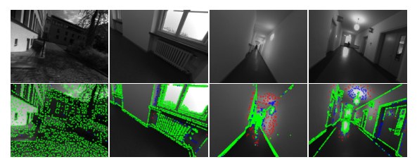
Figure 9. Candidate selection. The top row shows the original images, the bottom row shows the points chosen as candidates to be added to the map (2000 in each frame). Points selected on the first pass are shown in green, those selected on the second and third pass in blue and red respectively. Green candidates are evenly spread across gradient-rich areas, while points added on the second and third pass also cover regions with very weak intensity variations, but are much sparser.
图 9:候选点选取。上一行是原始图像,下一行是选来加入地图的候选点(每帧 2000 个)。第一轮选出的点为绿色,第二、三轮分别为蓝、红。绿色候选点均匀分布在梯度丰富的区域;后两轮补上的点也会覆盖强度变化很弱的区域,但稀疏得多。
Step 2: Candidate Point Tracking.
Point candidates are tracked in subsequent frames using a discrete search along the epipolar line, minimizing the photometric error (4). From the best match we compute a depth and associated variance, which is used to constrain the search interval for the subsequent frame. This tracking strategy is inspired by LSD-SLAM. Note that the computed depth only serves as initialization once the point is activated.
步骤 2:候选点跟踪。
候选点在后续帧中沿极线做离散搜索来跟踪,目标是最小化光度误差 (4)。由最佳匹配计算深度及相应方差,用来约束下一帧的搜索区间。这一跟踪策略受到 LSD-SLAM 的启发。注意,算出的深度只在点被激活时作为初值使用。
Step 3: Candidate Point Activation.
After a set of old points is marginalized, new point candidates are activated to replace them. Again, we aim at maintaining a uniform spatial distribution across the image. To this end, we first project all active points onto the most recent keyframe. We then activate candidate points which – also projected into this keyframe – maximize the distance to any existing point (requiring larger distance for candidates created during the second or third block-run). Figure 7 shows the resulting distribution of points in a number of scenes.
步骤 3:候选点激活。
一组旧点被边缘化之后,会激活新的候选点来替换它们。同样,我们希望在图像上保持均匀的空间分布。为此,先把所有活跃点投影到最新关键帧上,再激活那些——同样投影到该关键帧后——与任何已有点距离最大的候选点(对第二、三轮分块产生的候选,要求更大的距离)。图 7 给出了若干场景中由此得到的点分布。
Outlier and Occlusion Detection.
Since the available image data generally contains much more information than can be used in real time, we attempt to identify and remove potential outliers as early as possible. First, when searching along the epipolar line during candidate tracking, points for which the minimum is not sufficiently distinct are permanently discarded, greatly reducing the number of false matches in repetitive areas. Second, point observations for which the photometric error (4) surpasses a threshold are removed. The threshold is continuously adapted with respect to the median residual in the respective frame. For “bad” frames (e.g., frames that contain a lot of motion blur), the threshold will be higher, such that not all observations are removed. For good frames, in turn, the threshold will be lower, as we can afford to be more strict.
外点与遮挡检测。
由于可用的图像数据通常包含远超实时所能使用的信息,我们尽量尽早识别并去掉潜在外点。第一,在候选跟踪沿极线搜索时,若极小不够显著,该点就被永久丢弃,从而大幅减少重复区域中的错误匹配。第二,光度误差 (4) 超过某一阈值的点观测会被去掉。该阈值相对相应帧中残差的中位数持续调整。对“较差”的帧(例如含有大量运动模糊的帧),阈值会更高,以免所有观测都被去掉。反过来,对较好的帧,阈值会更低,因为这时可以更严格。
4 Results
4 结果
In this section we will extensively evaluate our Direct Sparse mono-VO algorithm (DSO). We both compare it to other monocular SLAM / VO methods, as well as evaluate the effect of important design and parameter choices. We use three datasets for evaluation:
本节将充分评测我们的直接稀疏单目视觉里程计算法(DSO,Direct Sparse mono-VO)。我们既把它与其他单目 SLAM / VO 方法比较,也评测重要设计和参数选择的影响。评测使用三个数据集:
(1) The TUM monoVO dataset [8], which provides 50 photometrically calibrated sequences, comprising 105 minutes of video recorded in dozens of different environments, indoors and outdoors (see Figure 11). Since the dataset only provides loop-closure-ground-truth (allowing to evaluate tracking accuracy via the accumulated drift after a large loop), we evaluate using the alignment error () as defined in the respective publication.
(1)TUM monoVO 数据集 [8],提供 50 条经过光度标定的序列,共 105 分钟视频,录制于数十种不同的室内外环境(见图 11)。由于该数据集只提供回环真值(因而可以通过大回环之后的累积漂移来评测跟踪精度),我们采用相应论文中定义的对齐误差()来评测。
(2) The EuRoC MAV dataset [1], which contains 11 stereo-inertial sequences comprising 19 minutes of video, recorded in 3 different indoor environments. For this dataset, no photometric calibration or exposure times are available, hence we omit photometric image correction and set (). We evaluate in terms of the absolute trajectory error (), which is the translational RMSE after alignment. For this dataset we crop the beginning of each sequence since they contain very shaky motion meant to initialize the IMU biases – we only use the parts of the sequence where the MAV is in the air.
(2)EuRoC MAV 数据集 [1],包含 11 条立体–惯性序列,共 19 分钟视频,录制于 3 种不同的室内环境。该数据集没有光度标定或曝光时间,因此我们省略光度图像校正,并令()。评测指标是绝对轨迹误差(),也就是做 对齐后的平移 RMSE。对该数据集,我们裁掉每条序列的开头,因为其中含有意在初始化 IMU 偏置的剧烈抖动运动——我们只使用飞行器已升空的那一部分。
(3) The ICL-NUIM dataset [10], which contains 8 ray-traced sequences comprising 4.5 minutes of video, from two indoor environments. For this dataset, photometric image correction is not required, and all exposure times can be set to . Again, we evaluate in terms of the absolute trajectory error ().
(3)ICL-NUIM 数据集 [10],包含 8 条光线追踪序列,共 4.5 分钟视频,来自两个室内环境。对该数据集不需要光度图像校正,全部曝光时间可设为 。同样,我们用绝对轨迹误差()来评测。
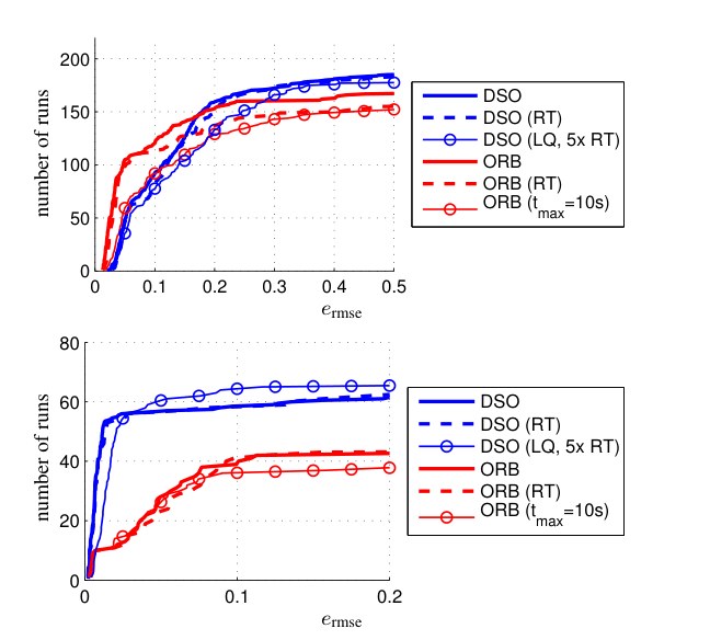
Figure 10. Results on EuRoC MAV (top) and ICL NUIM (bottom) datasets. Translational RMSE after Sim(3) alignment. RT (dashed) denotes hard-enforced real-time execution. Further, we evaluate DSO with low settings at 5 times real-time speed, and ORB-SLAM when restricting local loop-closures to points that have been observed at least once within the last s.
图 10:EuRoC MAV(上)和 ICL NUIM(下)数据集上的结果。做 Sim(3) 对齐后的平移 RMSE。RT(虚线)表示强制实时运行。我们还评测了低参数设置、以 5 倍实时速度运行的 DSO,以及把局部回环限制为最近 秒内至少被观测过一次的点时的 ORB-SLAM。
Methodology.
We aim at an evaluation as comprehensive as possible given the available data, and thus run all sequences both forwards and backwards, 5 times each (to account for non-deterministic behaviour). On default settings, we run each method 10 times each. For the EuRoC MAV dataset we further run both the left and the right video separately. In total, this gives 500 runs for the TUM-monoVO dataset, 220 runs for the EuRoC MAV dataset, and 80 runs for the ICL-NUIM dataset, which we run on 20 dedicated workstations. We remove the dependency on the host machine’s CPU speed by not enforcing real-time execution, except where stated otherwise: for ORB-SLAM we play the video at 20% speed, whereas DSO is run in a sequentialized, single-threaded implementation that runs approximately four times slower than real time. Note that even though we do not enforce real-time execution for most of the experiments, we use the exact same parameter settings as for the real-time comparisons.
方法。
在现有数据允许的范围内,我们希望评测尽可能全面,因此把所有序列既向前又向后各跑 5 次(以计入非确定性)。默认设置下,每种方法各跑 10 次。对 EuRoC MAV 数据集,我们还把左、右目视频分别跑一遍。合计起来,TUM-monoVO 有 500 次运行,EuRoC MAV 有 220 次,ICL-NUIM 有 80 次,分布在 20 台专用工作站上。为去掉对宿主机器 CPU 速度的依赖,除另行说明外我们不强制实时执行:对 ORB-SLAM,视频以 20% 速度播放;DSO 则用顺序化的单线程实现来跑,大约比实时慢四倍。需要注意,尽管多数实验并不强制实时,我们使用的参数设置与实时比较时完全相同。
The results are summarized in the form of cumulative error plots (see, e.g., Figure 10), which visualize for how many tracked sequences the respective error value ( / ) was below a certain threshold; thereby showing both accuracy on sequences where a method works well, as well as robustness, i.e., on how many sequences the method does not fail. The raw tracking results for all runs -- as well as scripts to compute the figures -- are provided in the supplementary material^2. Additional interesting analysis using the TUM-monoVO dataset – e.g. the influence of the camera’s field of view, the image resolution or the camera’s motion direction – can be found in [8].
结果以累积误差曲线的形式汇总(例如见图 10),它显示有多少条被跟踪的序列,其相应误差( / )低于某一阈值;从而既表现方法在效果好的序列上的精度,也表现鲁棒性,也就是方法在多少条序列上没有失败。全部运行的原始跟踪结果——以及用于计算这些图的脚本——在补充材料中提供^2。利用 TUM-monoVO 数据集所做的其他有意思的分析——例如相机视场、图像分辨率或相机运动方向的影响——可见 [8]。
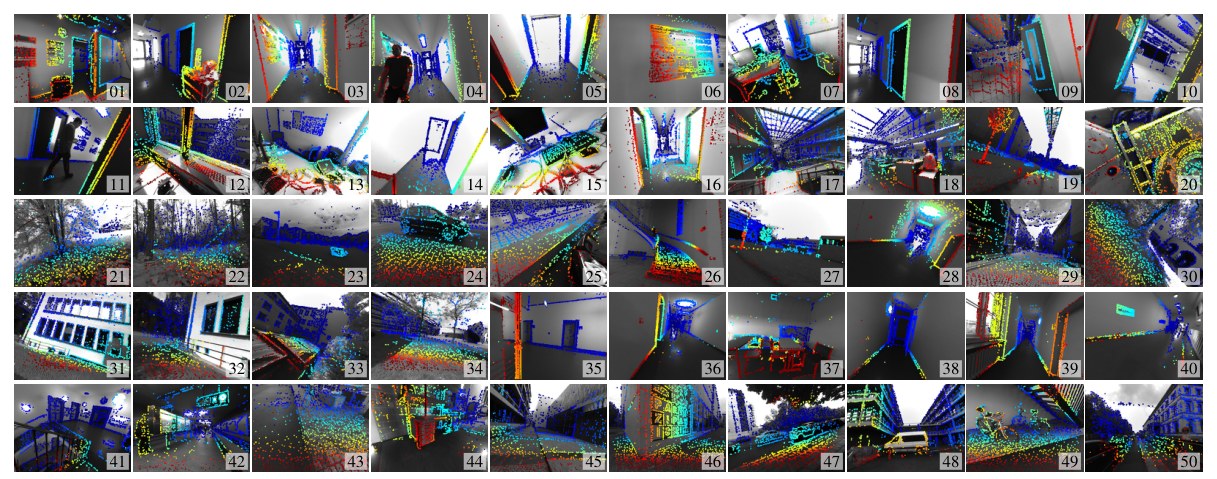
Figure 11. TUM mono-VO Dataset. A single image from each of the 50 TUM mono-VO dataset sequences (s_01 to s_50) used for evaluation and parameter studies, overlayed with the predicted depth map from DSO. The full dataset contains over 105 minutes of video (190'000 frames). Note the wide range of environments covered, ranging from narrow indoor corridors to wide outdoor areas, including forests.
图 11:TUM mono-VO 数据集。评测与参数研究用到的 50 条 TUM mono-VO 序列(s_01 到 s_50)各取一帧,并叠上 DSO 预测的深度图。全集超过 105 分钟视频(190'000 帧)。注意覆盖的环境很广,从狭窄的室内走廊到开阔的户外,也包括树林。
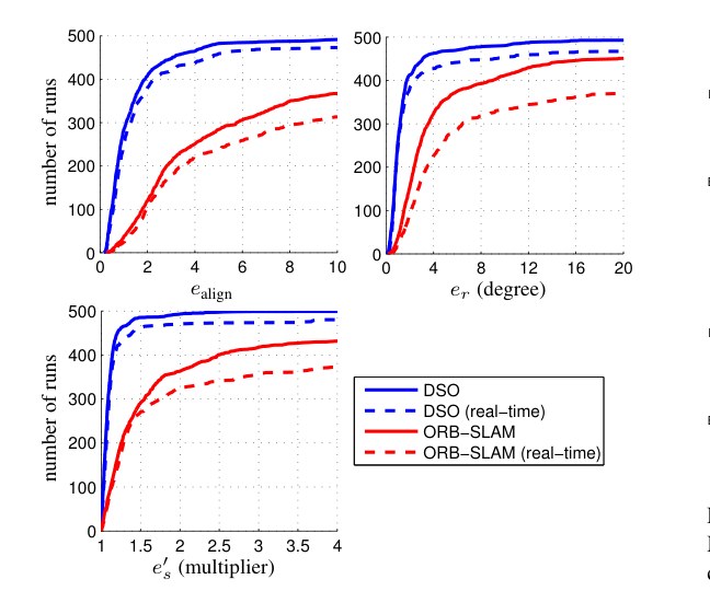
Figure 12. Results on TUM-monoVO dataset. Accumulated rotational drift and scale drift after a large loop, as well as the alignment error as defined in [8]. Since is a multiplicative factor, we aggregate . The solid line corresponds to sequentialized, non-real-time execution, the dashed line to hard enforced real-time processing. For DSO, we also show results obtained at low parameter settings, running at 5 times real-time speed.
图 12:TUM-monoVO 数据集上的结果。大回环之后累积的旋转漂移 与尺度漂移 ,以及 [8] 中定义的对齐误差。由于 是乘性因子,我们汇总为 。实线对应顺序执行、非实时;虚线对应强制实时。对 DSO,我们还给出了低参数设置、以 5 倍实时速度运行的结果。
Evaluated Methods and Parameter Settings.
We compare our method to the open-source implementation of (monocular) ORB-SLAM [20]. We also attempted to evaluate against the open-source implementations of LSD-SLAM [5] and SVO [9], however both methods consistently fail on most of the sequences. A major reason for this is that they assume brightness constancy (ignoring exposure changes), while both real-world datasets used contain heavy exposure variations.
评测方法与参数设置。
我们把方法与(单目)ORB-SLAM [20] 的开源实现比较。也曾尝试与 LSD-SLAM [5] 和 SVO [9] 的开源实现比较,但这两种方法在大多数序列上持续失败。一个主要原因是它们假设亮度恒定(忽略曝光变化),而所用的两个真实世界数据集都含有强烈的曝光变化。
To facilitate a fair comparison and allow application of the loop-closure metric from the TUM-monoVO dataset, we disable explicit loop-closure detection and re-localization for ORB-SLAM. Note that everything else (including local and global BA) remains unchanged, still allowing ORB-SLAM to detect incremental loop-closures that can be found via the co-visibility representation alone. All parameters are set to the same value across all sequences and datasets. The only exception is the ICL-NUIM dataset: For this dataset we set for DSO, and lower the FAST threshold for ORB-SLAM to 2, which we found to give best results.
为便于公平比较,并能够使用 TUM-monoVO 数据集的回环度量,我们关闭了 ORB-SLAM 的显式回环检测与重定位。注意其余一切(包括局部和全局束调整)保持不变,因而 ORB-SLAM 仍能检测仅通过共视表示即可发现的增量回环。所有参数在全部序列和数据集上取相同值。唯一例外是 ICL-NUIM 数据集:对该数据集,我们把 DSO 的 设为 3,并把 ORB-SLAM 的 FAST 阈值降到 2,我们发现这样效果最好。
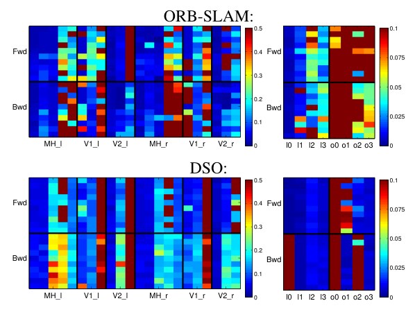
Figure 13. Full evaluation results. All error values for the EuRoC MAV dataset (left) and the ICL NUIM dataset (right): Each square corresponds to the (color-coded) absolute trajectory error over the full sequence. We run each of the 11 + 8 sequences (horizontal axis) forwards (“Fwd”) and backwards (“Bwd”), 10 times each (vertical axis); for the EuRoC MAV dataset we further use the left and the right image stream. Figure 10 shows these error values aggregated as cumulative error plot (bold, continuous lines).
图 13:完整评测结果。EuRoC MAV 数据集(左)和 ICL NUIM 数据集(右)的全部误差:每个方格对应整条序列上(伪彩色的)绝对轨迹误差 。11 + 8 条序列(横轴)各向前(“Fwd”)和向后(“Bwd”)跑 10 次(纵轴);EuRoC MAV 还分别使用左、右目图像流。图 10 把这些误差汇总成累积误差曲线(粗实线)。
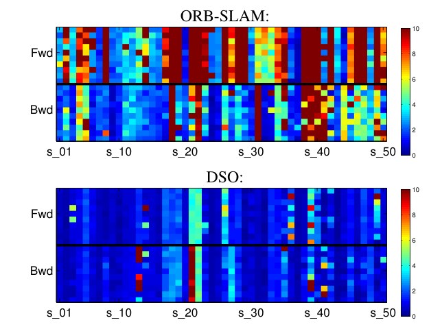
Figure 14. Full evaluation results. All error values for the TUM-monoVO dataset (also see Figure 11). Each square corresponds to the (color-coded) alignment error , as defined in [8]. We run each of the 50 sequences (horizontal axis) forwards (“Fwd”) and backwards (“Bwd”), 10 times each (vertical axis). Figure 12 shows all these error values aggregated as cumulative error plot (bold, continuous lines).
图 14:完整评测结果。TUM-monoVO 数据集上的全部误差(亦可参见图 11)。每个方格对应 [8] 中定义的(伪彩色)对齐误差 。50 条序列(横轴)各向前(“Fwd”)和向后(“Bwd”)跑 10 次(纵轴)。图 12 把这些误差汇总成累积误差曲线(粗实线)。
4.1 Quantitative Comparison
4.1 定量比较
Figure 10 shows the absolute trajectory RMSE on the EuRoC MAV dataset and the ICL-NUIM dataset for both methods (if an algorithm gets lost within a sequence, we set ). Figure 12 shows the alignment error , as well as the rotation-drift and scale-drift for the TUM-monoVO dataset.
图 10 给出了两种方法在 EuRoC MAV 数据集和 ICL-NUIM 数据集上的绝对轨迹 RMSE (若算法在某条序列中跟丢,我们令 )。图 12 给出了 TUM-monoVO 数据集上的对齐误差 ,以及旋转漂移 和尺度漂移 。
In addition to the non-real-time evaluation (bold lines), we evaluate both algorithms in a hard-enforced real-time setting on an Intel i7-4910MQ CPU (dashed lines). The direct, sparse approach clearly outperforms ORB-SLAM in accuracy and robustness both on the TUM-monoVO dataset, as well as the synthetic ICL_NUIM dataset. On the EuRoC MAV dataset, ORB-SLAM achieves a better accuracy (but lower robustness). This is due to two major reasons: (1) there is no photometric calibration available, and (2) the sequences contain many small loops or segments where the quadrocopter “back-tracks” the way it came, allowing ORB-SLAM’s local mapping component to implicitly close many small and some large loops, whereas our visual odometry formulation permanently marginalizes all points and frames that leave the field of view. We can validate this by prohibiting ORB-SLAM from matching against any keypoints that have not been observed for more than s (lines with circle markers in Figure 10): In this case, ORB-SLAM performs similar to DSO in terms of accuracy, but is less robust. The slight difference in robustness for DSO comes from the fact that for real-time execution, tracking new frames and keyframe-creation are parallelized, thus new frames are tracked on the second-latest keyframe, instead of the latest. In some rare cases – in particular during strong exposure changes – this causes initial image alignment to fail.
除了非实时评测(粗线)之外,我们还在 Intel i7-4910MQ CPU 上对两种算法做强制实时评测(虚线)。在 TUM-monoVO 数据集以及合成的 ICL-NUIM 数据集上,这种直接、稀疏的方法在精度和鲁棒性上都明显优于 ORB-SLAM。在 EuRoC MAV 数据集上,ORB-SLAM 取得了更好的精度(但鲁棒性较低)。这主要有两个原因:(1)没有可用的光度标定;(2)序列中包含许多小回环,或飞行器沿来路“折返”的片段,使得 ORB-SLAM 的局部建图能够隐式合上许多小回环和一些大回环,而我们的视觉里程计表述会把离开视野的点和帧永久边缘化。我们可以这样验证这一点:禁止 ORB-SLAM 匹配超过 秒未见过的任何关键点(图 10 中带圆圈标记的线):这时 ORB-SLAM 的精度与 DSO 相近,但鲁棒性较差。DSO 在鲁棒性上的轻微差别,来自实时执行时跟踪新帧与创建关键帧是并行的,因而新帧是在倒数第二个关键帧而不是最新关键帧上跟踪的。在少数情形——尤其是曝光剧烈变化时——这会导致初始图像对齐失败。
To show the flexibility of DSO, we include results when running at 5 times real-time speed[^3], with reduced settings (=800 points, =6 active frames, image resolution, Gauss-Newton iterations after a keyframe is created): Even with such extreme settings, DSO achieves very good accuracy and robustness on all three datasets.
[^3]: All images are loaded, decoded, and pinhole-rectified beforehand.
为展示 DSO 的灵活性,我们还给出了以 5 倍实时速度运行、并降低设置时的结果^3(=800 个点,=6 个活跃帧, 的图像分辨率,创建关键帧后高斯–牛顿迭代不超过 4 次):即使在这样极端的设置下,DSO 在全部三个数据集上仍然取得很好的精度和鲁棒性。
Note that DSO is designed as a pure visual adometry while ORB-SLAM constitutes a full SLAM system, including loop-closure detection & correction and re-localization – all these additional abilities are neglected or switched off in this comparison.
需要注意,DSO 被设计成纯粹的视觉里程计,而 ORB-SLAM 是完整的 SLAM 系统,包括回环检测与纠正以及重定位——在本比较中,这些额外能力都被忽略或关闭。
4.2 Parameter Studies
4.2 参数研究
This section aims at evaluating a number of different parameter and algorithm design choices, using the TUM-monoVO dataset.
本节旨在利用 TUM-monoVO 数据集,评测若干不同的参数和算法设计选择。
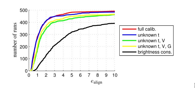
Figure 15. Photometric calibration. Errors on the TUM-monoVO dataset, when incrementally disabling photometric calibration.
图 15:光度标定。在 TUM-monoVO 数据集上,逐步关闭光度标定各项时的误差。
Photometric Calibration.
We analyze the influence of photometric calibration, verifying that it in fact increases accuracy and robustness: to this end, we incrementally disable the different components:
光度标定。
我们分析光度标定的影响,以验证它确实提高精度和鲁棒性:为此,我们逐步关闭其中的不同成分:
- exposure (blue): set and .
- 曝光(蓝):令 且 。
- vignette (green): set (and 1.).
- 暗角(绿):令 (并包含第 1 项)。
- response (yellow): set (and 1 – 2.).
- 响应(黄):令 (并包含第 1–2 项)。
- brightness constancy (black): set , i.e., disable affine brightness correction (and 1 – 3.).
- 亮度恒定(黑):令 ,也就是关闭仿射亮度校正(并包含第 1–3 项)。
Figure 15 shows the result. While known exposure times seem to have little effect on the accuracy, removing vignette and response calibration does slightly decrease the overall accuracy and robustness. Interestingly, only removing vignette calibration performs slightly worse than removing vignette and response calibration. A naïve brightness constancy assumption (as used in many other direct approaches like LSD-SLAM or SVO) clearly performs worst, since it does not account for automatic exposure changes at all.
图 15 给出了结果。已知曝光时间似乎对精度影响不大,但去掉暗角和响应校正会略微降低整体精度和鲁棒性。有意思的是,只去掉暗角校正,表现比同时去掉暗角和响应校正还略差。朴素的亮度恒定假设(LSD-SLAM 或 SVO 等许多其他直接法所采用的)明显最差,因为它完全不考虑自动曝光变化。
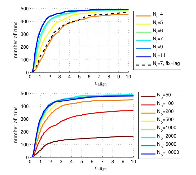
Figure 16. Amount of data used. Errors on the TUM-monoVO dataset, when changing the size of the optimization window (top) and the number of points (bottom). Using more than points or active frames has only marginal impact. Note that as real-time default setting, we use and , mainly to obtain denser reconstructions.
图 16:所用数据量。在 TUM-monoVO 数据集上,改变优化窗口大小(上)和点数(下)时的误差。点数超过 、或活跃帧数超过 之后,影响已经很小。实时默认设置采用 、,主要是为了得到更密的重建。
Amount of Data.
We analyze the effect of changing the amount of data used, by varying the number of active points , as well as the number of frames in the active window . Note that increasing allows to keep more observations per point: For any point we only ever keep observations in active frames; thus the number of observations when marginalizing a point is limited to (see Section 2.3). Figure 16 summarizes the result. We can observe that the benefit of simply using more data quickly flattens off after points. At the same time, the number of active frames has little influence after , while increasing the runtime quadratically. We further evaluate a fixed-lag marginalization strategy (i.e., always marginalize the oldest keyframe, instead of using the proposed distancescore) as in [17]: this performs significantly worse.
数据量。
我们通过分析改变所用数据量的影响,办法是改变活跃点数 ,以及活跃窗口中的帧数 。注意,增大 可以让每个点保留更多观测:对任意一点,我们只保留活跃帧中的观测;因而在边缘化一个点时,观测数以 为上限(见第 2.3 节)。图 16 汇总了结果。可以看到,仅仅使用更多数据的收益在 个点之后很快变平。与此同时,活跃帧数在 之后影响已经很小,而运行时间却按二次增长。我们还评测了固定滞后的边缘化策略(也就是总是边缘化最旧的关键帧,而不是使用所提出的距离分数),做法同 [17]:这明显更差。
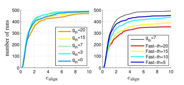
Figure 17. Selection of data used. Errors on the TUM-monoVO dataset, when changing the type of data used. Left: Errors for different gradient thresholds , which seems to have a limited impact on the algorithm’s accuracy. Right: Errors when only using FAST corners, at different thresholds. Using only FAST corners significantly reduces accuracy and robustness, showing that the ability to use data from edges and weakly textured surfaces does have a real benefit.
图 17:所用数据的选取。在 TUM-monoVO 数据集上,改变所用数据类型时的误差。左:不同梯度阈值 下的误差,对算法精度的影响似乎有限。右:只使用 FAST 角点、并改变其阈值时的误差。只用 FAST 角点会明显降低精度和鲁棒性,说明利用边缘和弱纹理表面的数据确实有好处。
Selection of Data.
In addition to evaluating the effect of the number of residuals used, it is interesting to look at which data is used – in particular since one of the main benefits of a direct approach is the ability to sample from all points, instead of only using corners. To this end, we vary the gradient threshold for point selection, ; the result is summarized in Figure 17. While there seems to be a sweet spot around (if is too large, for some scenes not enough well-distributed points are available to sample from – if it is too low, too much weight will be given to data with a low signal-to-noise ratio), the overall impact is relatively low.
数据选取。
除了评测所用残差数量的影响,看一看用了哪些数据也很有意思——尤其是因为直接法的一个主要好处,就是能够从所有点中取样,而不是只用角点。为此,我们改变选点的梯度阈值 ;结果汇总在图 17 中。似乎在 附近有一个较优点(若 太大,有些场景就没有足够、分布良好的点可供取样——若太低,又会给信噪比低的数据过多权重),但总体影响相对较小。
More interestingly, we analyse the effect of only using corners, by restricting point candidates to FAST corners only. We can clearly see that only using corners significantly decreases performance. Note that for lower FAST thresholds, many false “corners” will be detected along edges, which our method can still use, in contrast to indirect methods for which such points will be outliers. In fact, ORB-SLAM achieves best performance using the default threshold of 20.
更有意思的是,我们分析了只用角点的影响,办法是把候选点限制为 FAST 角点。可以清楚地看到,只用角点会显著降低性能。注意,在较低的 FAST 阈值下,沿边缘会检测出许多虚假“角点”,我们的方法仍然可以利用它们,而间接法会把这些点当作外点。事实上,ORB-SLAM 在默认阈值 20 时取得最佳性能。
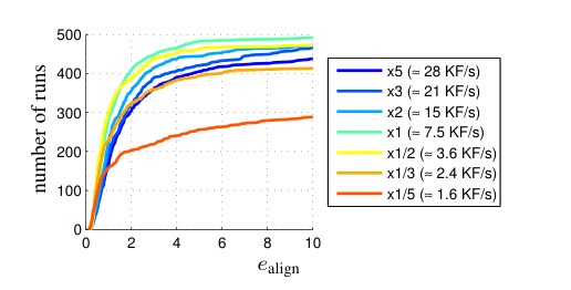
Figure 18. Number of keyframes. Errors on the TUM-monoVO dataset, when changing the number of keyframes taken via the threshold .
图 18:关键帧数量。在 TUM-monoVO 数据集上,通过阈值 改变所取关键帧数量时的误差。
Number of Keyframes.
We analyze the number of keyframes taken by varying (see Section 3.1). For each value of we give the resulting average number of keyframes per second; the default setting results in 8 keyframes per second, which is easily achieved in real time. The result is summarized in Figure 18. Taking too few keyframes (less than 4 per second) reduces the robustness, mainly in situations with strong occlusions / dis-occlusions, e.g., when walking through doors. Taking too many keyframes, on the other hand (more than 15 per second), decreases accuracy. This is because taking more keyframes causes them to be marginalized earlier (since is fixed), thereby accumulating linearizations around earlier (and less accurate) linearization points.
关键帧数量。
我们通过改变 来分析所取关键帧的数量(见第 3.1 节)。对每个 值,我们给出由此得到的平均每秒关键帧数;默认设置 约为每秒 8 个关键帧,这在实时下很容易达到。结果汇总于图 18。关键帧太少(每秒不足 4 个)会降低鲁棒性,主要出现在遮挡 / 去遮挡很强的情形,例如走过门时。另一方面,关键帧太多(每秒超过 15 个)会降低精度。这是因为取更多关键帧会使它们更早被边缘化(因为 是固定的),从而在更早(也更不准)的线性化点附近累积线性化。
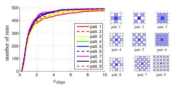
Figure 19. Residual pattern. Errors on the TUM-monoVO dataset for some of the evaluated patterns . Using only a neighborhood seems to perform slightly worse – using more than the proposed 8-pixel pattern however seems to have little benefit – at the same time, using a larger neighbourhood increases the computational demands. Note that these results may vary with low-level properties of the used camera and lens, such as the point spread function.
图 19:残差图案。TUM-monoVO 数据集上,若干被评测图案 的误差。只用 邻域似乎略差一些——但超过文中提出的 8 像素图案之后,收益已经不大——同时,更大的邻域会增加计算量。注意这些结果可能随所用相机和镜头的底层特性(例如点扩散函数)而变化。
Residual Pattern.
We test different residual patterns for , covering smaller or larger areas. The result is shown in Figure 19.
残差图案。
我们为 测试了覆盖更小或更大区域的不同残差图案。结果见图 19。
4.3 Geometric vs. Photometric Noise Study
4.3 几何噪声与光度噪声研究
The fundamental difference between the proposed direct model and the indirect model is the noise assumption. The direct approach models photometric noise, i.e., additive noise on pixel intensities. In contrast, the indirect approaches models geometric noise, i.e., additive noise on the -position of a point in the image plane, assuming that keypoint descriptors are robust to photometric noise. It therefore comes at no surprise that the indirect approach is significantly more robust to geometric noise in the data. In turn, the direct approach performs better in the presence of strong photometric noise – which keypoint-descriptors (operating on a purely local level) fail to filter out. We verify this by analyzing tracking accuracy on the TUM-monoVO dataset, when artificially adding (a) geometric noise, and (b) photometric noise to the images.
所提出的直接模型与间接模型的根本差别,在于噪声假设。直接法建模的是光度噪声,也就是像素强度上的加性噪声。相反,间接法建模的是几何噪声,也就是图像平面中一个点 位置上的加性噪声,并假定关键点描述子对光度噪声是鲁棒的。因此,间接法对数据中的几何噪声明显更鲁棒,也就不足为奇。反过来,在强光度噪声下直接法表现更好——关键点描述子(只在纯局部层面工作)无法滤掉这种噪声。我们通过在 TUM-monoVO 数据集上人为加入(a)几何噪声和(b)光度噪声,分析跟踪精度,来验证这一点。
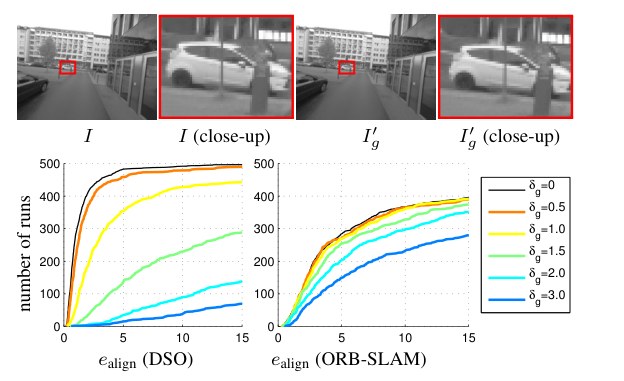
Figure 20. Geometric noise. Effect of applying low-frequency geometric noise to the image, simulating geometric distortions such as a rolling shutter (evaluated on the TUM-monoVO dataset). The top row shows an example image with . While the effect is hardly visible to the human eye (observe that the close-up is slightly shifted), it has a severe impact on SLAM accuracy, in particular when using a direct model. Note that the distortion caused by a standard rolling shutter camera easily surpasses .
图 20:几何噪声。对图像施加低频几何噪声、以模拟卷帘快门这类几何畸变的影响(在 TUM-monoVO 数据集上评测)。上一行是 时的示例图像。人眼几乎看不出差别(放大后可见有轻微错位),却会严重损害 SLAM 精度,对直接法尤其如此。注意,普通卷帘快门相机造成的畸变很容易超过 。
Geometric Noise.
For each frame, we separately generate a low-frequency random flow-map by up-sampling a grid filled with uniformly distributed random values from (using bicubic interpolation). We then perturb the original image by shifting each pixel by :
几何噪声。
对每一帧,我们单独生成一张低频随机流动图 ,办法是对填满 上均匀随机值的 网格做上采样(使用双三次插值)。然后把原图中每个像素 平移 ,以扰动图像:
This procedure simulates noise originating from (unmodeled) rolling shutter or inaccurate geometric camera calibration. Figure 20 visualizes an example of the resulting noise pattern, as well as the accuracy of ORB-SLAM and DSO for different values of . As expected, we can clearly observe how DSO’s performance quickly deteriorates with added geometric noise, whereas ORB-SLAM is much less affected. This is because the first step in the indirect pipeline – keypoint detection and extraction – is not affected by low-frequency geometric noise, as it operates on a purely local level. The second step then optimizes a geometric noise model – which not surprisingly deals well with geometric noise. In the direct approach, in turn, geometric noise is not modeled, and thus has a much more severe effect – in fact, for there likely exists no state for which all residuals are within the validity radius of the linearization of ; thus optimization fails entirely (which can be alleviated by using a coarser pyramid level). Note that this result also suggests that the proposed direct model is more susceptible to inaccurate intrinsic camera calibration than the indirect approach – in turn, it may benefit more from accurate, non-parametric intrinsic calibration.
这一步骤模拟来自(未建模的)卷帘快门或不准确几何相机标定的噪声。图 20 画出了由此得到的噪声图案示例,以及不同 下 ORB-SLAM 与 DSO 的精度。正如所料,可以清楚地看到,随着加入几何噪声,DSO 的性能迅速变差,而 ORB-SLAM 受影响小得多。这是因为间接法流程的第一步——关键点检测与提取——在纯局部层面工作,不受低频几何噪声影响。第二步再优化一个几何噪声模型——它理所当然地能够较好地处理几何噪声。反过来,直接法并不建模几何噪声,因而影响要严重得多——事实上,当 时,很可能不存在一个使所有残差都落在 的线性化有效半径之内的状态;于是优化彻底失败(改用更粗的金字塔层可以缓解)。需要注意,这一结果也表明,与间接法相比,所提出的直接模型对不准确的相机内参标定更敏感——反过来,它也可能从精确的非参数内参标定中受益更多。
Photometric Noise.
For each frame, we separately generate a high-frequency random blur-map by up-sampling a grid filled with uniformly distributed random values in . We then perturb the original image by adding anisotropic blur with standard deviation to pixel :
光度噪声。
对每一帧,我们单独生成一张高频随机模糊图 ,办法是对填满 上均匀随机值的 网格做上采样。然后对像素 加上标准差为 的各向异性模糊,以扰动原图:
where denotes a 2D Gaussian kernel with standard deviation . Figure 21 shows the result. We can observe that DSO is slightly more robust to photometric noise than ORB-SLAM – this is because (purely local) keypoint matching fails for high photometric noise, whereas a joint optimization of the photometric error better overcomes the introduced distortions.
其中 表示标准差为 的二维高斯核。图 21 给出了结果。可以看到,DSO 对光度噪声比 ORB-SLAM 略更鲁棒——这是因为(纯局部的)关键点匹配在高光度噪声下会失败,而对光度误差做联合优化更能克服所引入的畸变。
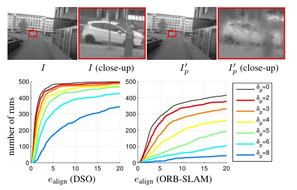
Figure 21. Photometric noise. Effect of applying high-frequent, non-isotropic blur to the image, simulating photometric noise (evaluated on the TUM-monoVO dataset). The top row shows an example image with , the effect is clearly visible. Since the direct approach models a photometric error, it is more robust to this type of noise than indirect methods.
图 21:光度噪声。对图像施加高频、非各向同性模糊,以模拟光度噪声(在 TUM-monoVO 数据集上评测)。上一行是 时的示例,效果清晰可见。由于直接法建模的是光度误差,对这类噪声比间接法更鲁棒。
To summarize: While the direct approach outperforms the indirect approach on well-calibrated data, it is ill-suited in the presence of strong geometric noise, e.g., originating from a rolling shutter or inaccurate intrinsic calibration. In practice, this makes the indirect model superior for smartphones or off-the-shelf webcams, since these were designed to capture videos for human consumption – prioritizing resolution and light-sensitivity over geometric precision. In turn, the direct approach offers superior performance on data captured with dedicated cameras for machine-vision, since these put more importance on geometric precision, rather than capturing appealing images for human consumption. Note that this can be resolved by tightly integrating the rolling shutter into the model, as done, e.g., in [19, 18, 15].
总结起来:在标定良好的数据上,直接法优于间接法;但在存在强几何噪声时——例如来自卷帘快门或不准确的内参标定——它并不适用。实践中,这使得间接模型更适合智能手机或现成的网络摄像头,因为这些设备被设计来拍摄供人观看的视频——优先考虑分辨率和感光,而不是几何精度。反过来,在为机器视觉专门采集的数据上,直接法表现更好,因为这类相机更看重几何精度,而不是拍出吸引人的画面。需要注意,若把卷帘快门紧密写进模型,这一问题可以解决,例如 [19, 18, 15] 所做的那样。
4.4 Qualitative Results
4.4 定性结果
In addition to accurate camera tracking, DSO computes 3D points on all gradient-rich areas, including edges – resulting in point-cloud reconstructions similar to the semi-dense reconstructions of LSD-SLAM. The density then directly corresponds to how many points we keep in the active window . Figure 22 shows some examples.
除了准确的相机跟踪,DSO 还在所有梯度丰富的区域(包括边缘)上计算三维点——得到的点云重建类似于 LSD-SLAM 的半稠密重建。密度则直接对应我们在活跃窗口中保留的点数 。图 22 给出了一些例子。
Figure 23 shows three more scenes (one from each dataset), together with some corresponding depth maps. Note that our approach is able to track through scenes with very little texture, whereas indirect approaches fail. All reconstructions shown are simply accumulated from the odometry, without integrating loop-closures. See the supplementary video for more qualitative results.
图 23 另外给出三个场景(每个数据集各一个),以及若干相应的深度图。注意,我们的方法能够在纹理极少的场景中完成跟踪,而间接法会失败。所示的全部重建都只是从里程计累积而来,没有加入回环。更多定性结果见补充视频。
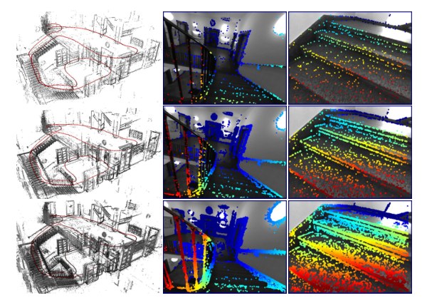
Figure 22. Point density. 3D point cloud and some coarse depth maps, i.e., the most recent keyframe with all active points projected into it) for =500 (top), =2000 (middle), and =10000 (bottom).
图 22:点密度。三维点云以及若干较粗的深度图,也就是把全部 个活跃点投影到最新关键帧上的结果:=500(上)、=2000(中)、=10000(下)。
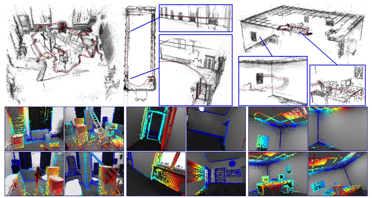
Figure 23. Qualitative examples. One scene from each dataset (left to right: V2_01_easy [1], seq_38 [8] and office_1 [10]), computed in real time with default settings. The bottom shows some corresponding (sparse) depth maps – some scenes contain very little texture, making them very challenging for indirect approaches.
图 23:定性示例。三个数据集各取一个场景(从左到右:V2_01_easy [1]、seq_38 [8] 和 office_1 [10]),用默认设置实时计算。底部是若干对应的(稀疏)深度图——有的场景纹理极少,对间接法非常困难。
5 Conclusion
5 结论
We have presented a novel direct and sparse formulation for Structure from Motion. It combines the benefits of direct methods (seamless ability to use & reconstruct all points instead of only corners) with the flexibility of sparse approaches (efficient, joint optimization of all model parameters). This is possible in real time by omitting the geometric prior used by other direct methods, and instead evaluating the photometric error for each point over a small neighborhood of pixels, to well-constrain the overall problem. Furthermore, we incorporate full photometric calibration, completing the intrinsic camera model that traditionally only reflects the geometric component of the image formation process.
我们提出了一种新的、用于运动恢复结构的直接且稀疏表述。它把直接法的好处(可以自然地使用并重建所有点,而不只是角点)与稀疏方法的灵活性(对全部模型参数做高效的联合优化)结合起来。之所以能实时完成,是因为我们去掉了其他直接法使用的几何先验,改为对每个点在一个小像素邻域上计算光度误差,以便把整体问题约束住。此外,我们纳入了完整的光度标定,补全了传统上只反映成像过程几何部分的内参相机模型。
We have implemented our direct & sparse model in the form of a monocular visual odometry algorithm (DSO), incrementally marginalizing / eliminating old states to maintain real-time performance. To this end we have developed a front-end that performs data-selection and provides accurate initialization for optimizing the highly non-convex energy function. Our comprehensive evaluation on several hours of video shows the superiority of the presented formulation relative to state-of-the-art indirect methods. We furthermore present an exhaustive parameter study, indicating that (1) simply using more data does not increase tracking accuracy (although it makes the 3D models denser), (2) using all points instead of only corners does provide a real gain in accuracy and robustness, and (3) incorporating photometric calibration does increase performance, in particular compared to the basic “brightness constancy” assumption.
我们把这一直接且稀疏的模型实现为一套单目视觉里程计算法(DSO),通过逐步边缘化 / 消去旧状态来保持实时性能。为此,我们开发了一个负责选取数据、并为优化高度非凸的能量函数提供准确初值的前端。在数小时视频上的全面评测表明,相对最先进的间接法,所提出的表述更优。我们还做了详尽的参数研究,表明:(1)仅仅使用更多数据并不会提高跟踪精度(虽然会让三维模型更密);(2)使用全部点而不是只用角点,确实能带来精度和鲁棒性上的实际增益;(3)纳入光度标定确实能提高性能,尤其是相对于基本的“亮度恒定”假设。
We have also shown experimentally that the indirect approach – modeling a geometric error – is much more robust to geometric noise, e.g., originating from a poor intrinsic camera calibration or a rolling shutter. The direct approach is in turn more robust to photometric noise, and achieves superior accuracy on well-calibrated data. We believe this to be one of the main explanations for the recent revival of direct formulations after a dominance of indirect approaches for more than a decade: For a long time, the predominant source of digital image data were cameras, which originally were designed to capture images for human viewing (such as off-the-shelf webcams or integrated smartphone cameras). In this setting, the strong geometric distortions caused by rolling shutters and imprecise lenses favored the indirect approach. In turn, with 3D computer vision becoming an integral part of mass-market products (including autonomous cars and drones, as well as mobile devices for VR and AR), cameras are being developed specifically for this purpose, featuring global shutters, precise lenses, and high frame-rates – which allows direct formulations to realize their full potential.
我们还用实验表明,间接法——建模几何误差——对几何噪声鲁棒得多,例如来自较差的相机内参标定或卷帘快门。直接法则对光度噪声更鲁棒,并在标定良好的数据上取得更高精度。我们认为,这是直接法表述在间接法主导十多年之后近来再度兴起的主要原因之一:在很长一段时间里,数字图像数据的主要来源是原本为人眼观看而设计的相机(例如现成的网络摄像头或集成在智能手机里的相机)。在这种设定下,卷帘快门和不精确镜头造成的强烈几何畸变更有利于间接法。反过来,随着三维计算机视觉成为大众市场产品的组成部分(包括自动驾驶汽车和无人机,以及用于 VR 和 AR 的移动设备),专门为此开发的相机开始出现,它们具有全局快门、精确镜头和高帧率——从而让直接法表述能够充分发挥潜力。
Since the structure of the proposed direct sparse energy formulation is the same as that of indirect methods, it can be integrated with other optimization frameworks like (double-windowed) bundle adjustment [25] or incremental smoothing and mapping [14]. The main challenge here is the greatly increased degree of non-convexity compared to the indirect model, which originates from the inclusion of the image in the error function – this is likely to restrict the use of our model to video processing.
由于所提出的直接稀疏能量表述与间接法具有相同的结构,它可以与其他优化框架集成,例如(双窗口)束调整 [25] 或增量平滑与建图 [14]。这里的主要挑战是,与间接模型相比,非凸程度大大增加,根源在于误差函数中包含了图像本身——这很可能把我们模型的使用限制在视频处理上。
References
[1] M. Burri, J. Nikolic, P. Gohl, T. Schneider, J. Rehder, S. Omari, M. Achtelik, and R. Siegwart. The EuRoC micro aerial vehicle datasets. International Journal of Robotics Research , 2016.
[2] D. Caruso, J. Engel, and D. Cremers. Large-scale direct SLAM for omnidirectional cameras. In International Conference on Intelligent Robot Systems (IROS) , 2015.
[3] J. Civera, A. Davison, and J. Montiel. Inverse depth parametrization for monocular SLAM. Transactions on Robotics , 24(5):932–945, 2008.
[4] A. Davison, I. Reid, N. Molton, and O. Stasse. MonoSLAM: Real-time single camera SLAM. Transactions on Pattern Analysis and Machine Intelligence (TPAMI) , 29, 2007.
[5] J. Engel, T. Schöps, and D. Cremers. LSD-SLAM: Large-scale direct monocular SLAM. In European Conference on Computer Vision (ECCV) , 2014.
[6] J. Engel, J. Stueckler, and D. Cremers. Large-scale direct slam with stereo cameras. In International Conference on Intelligent Robot Systems (IROS) , 2015.
[7] J. Engel, J. Sturm, and D. Cremers. Scale-aware navigation of a low-cost quadrocopter with a monocular camera. Robotics and Autonomous Systems (RAS) , 62(11):1646––1656, 2014.
[8] J. Engel, V. Usenko, and D. Cremers. A photometrically calibrated benchmark for monocular visual odometry. In arXiv preprint arXiv , 2016.
[9] C. Forster, M. Pizzoli, and D. Scaramuzza. SVO: Fast semi-direct monocular visual odometry. In International Conference on Robotics and Automation (ICRA) , 2014.
[10] A. Handa, T. Whelan, J. McDonald, and A. Davison. A benchmark for RGB-D visual odometry, 3D reconstruction and SLAM. In International Conference on Robotics and Automation (ICRA) , 2014.
[11] G. P. Huang, A. I. Mourikis, and S. I. Roumeliotis. A first-estimates Jacobian EKF for improving SLAM consistency. In International Symposium on Experimental Robotics , 2008.
[12] H. Jin, P. Favaro, and S. Soatto. Real-time 3-d motion and structure of point features: Front-end system for vision-based control and interaction. In International Conference on Computer Vision and Pattern Recognition (CVPR) , 2000.
[13] H. Jin, P. Favaro, and S. Soatto. A semi-direct approach to structure from motion. The Visual Computer , 19(6):377–394, 2003.
[14] M. Kaess, H. Johannsson, R. Roberts, V. Ila, J. Leonard, and F. Dellaert. iSAM2: Incremental smoothing and mapping using the Bayes tree. International Journal of Robotics Research , 31(2):217–236, Feb 2012.
[15] C. Kerl, J. Stueckler, and D. Cremers. Dense continuous-time tracking and mapping with rolling shutter RGB-D cameras. In International Conference on Computer Vision (ICCV) , 2015.
[16] G. Klein and D. Murray. Parallel tracking and mapping for small AR workspaces. In International Symposium on Mixed and Augmented Reality (ISMAR) , 2007.
[17] S. Leutenegger, S. Lynen, M. Bosse, R. Siegwart, and P. Furgale. Keyframe-based visual–inertial odometry using nonlinear optimization. International Journal of Robotics Research , 34(3):314–334, 2015.
[18] M. Li, B. Kim, and A. Mourikis. Real-time motion estimation on a cellphone using inertial sensing and a rolling-shutter camera. In International Conference on Robotics and Automation (ICRA) , 2013.
[19] S. Lovegrove, A. Patron-Perez, and G. Sibley. Spline fusion: A continuous-time representation for visual-inertial fusion with application to rolling shutter cameras. In British Machine Vision Converence (BMVC) , 2013.
[20] R. Mur-Artal, J. Montiel, and J. Tardos. ORB-SLAM: a versatile and accurate monocular SLAM system. Transactions on Robotics , 31(5):1147–1163, 2015.
[21] R. Newcombe, S. Lovegrove, and A. Davison. DTAM: Dense tracking and mapping in real-time. In International Conference on Computer Vision (ICCV) , 2011.
[22] M. Pizzoli, C. Forster, and D. Scaramuzza. REMODE: Probabilistic, monocular dense reconstruction in real time. In International Conference on Robotics and Automation (ICRA) , 2014.
[23] R. Ranftl, V. Vineet, Q. Chen, and V. Koltun. Dense monocular depth estimation in complex dynamic scenes. In International Conference on Computer Vision and Pattern Recognition (CVPR) , 2016.
[24] T. Schöps, J. Engel, and D. Cremers. Semi-dense visual odometry for AR on a smartphone. In International Symposium on Mixed and Augmented Reality (ISMAR) , 2014.
[25] H. Strasdat, A. J. Davison, J. M. M. Montiel, and K. Konolige. Double window optimisation for constant time visual SLAM. In International Conference on Computer Vision (ICCV) , 2011.
[26] J. Stühmer, S. Gumhold, and D. Cremers. Real-time dense geometry from a handheld camera. In Pattern Recognition (DAGM) , 2010.
[27] L. Valgaerts, A. Bruhn, M. Mainberger, and J. Weickert. Dense versus sparse approaches for estimating the fundamental matrix. International Journal of Computer Vision (IJCV) , 96(2):212–234, 2012.