Improving neural networks by preventing co-adaptation of feature detectors

通过防止特征检测器共适应来改进神经网络

G. E. Hinton ∗    N. Srivastava    A. Krizhevsky    I. Sutskever    R. R. Salakhutdinov Affiliation:  Department of Computer Science, University of Toronto, Affiliation:  6 King’s College Rd, Toronto, Ontario M5S 3G4, Canada Affiliation:  ∗ To whom correspondence should be addressed; E-mail: hinton@cs.toronto.edu

When a large feedforward neural network is trained on a small training set, it typically performs poorly on held-out test data. This “overfitting” is greatly reduced by randomly omitting half of the feature detectors on each training case. This prevents complex co-adaptations in which a feature detector is only helpful in the context of several other specific feature detectors. Instead, each neuron learns to detect a feature that is generally helpful for producing the correct answer given the combinatorially large variety of internal contexts in which it must operate. Random “dropout” gives big improvements on many benchmark tasks and sets new records for speech and object recognition.

当大型前馈神经网络在较小训练集上训练时，在留出测试数据上通常表现很差。这种「过拟合」可通过在每个训练样本上随机省略一半特征检测器而大幅减轻。这能防止复杂的共适应：某个特征检测器只在若干其他特定检测器同时存在时才有用。相反，每个神经元会学会检测一种特征，使其在必须面对的组合爆炸般的内部上下文中，大体上都能帮助给出正确答案。随机「dropout」在许多基准任务上带来大幅提升，并在语音与物体识别上刷新记录。

A feedforward, artificial neural network uses layers of non-linear “hidden” units between its inputs and its outputs. By adapting the weights on the incoming connections of these hidden units it learns feature detectors that enable it to predict the correct output when given an input vector [1]. If the relationship between the input and the correct output is complicated and the network has enough hidden units to model it accurately, there will typically be many different settings of the weights that can model the training set almost perfectly, especially if there is only a limited amount of labeled training data. Each of these weight vectors will make different predictions on held-out test data and almost all of them will do worse on the test data than on the training data because the feature detectors have been tuned to work well together on the training data but not on the test data.

前馈人工神经网络在输入与输出之间使用多层非线性「隐」单元。通过调整这些隐单元入边连接上的权重，它学会特征检测器，从而在给定输入向量时预测正确输出 [1]。若输入与正确输出之间的关系复杂，且网络有足够多隐单元可准确建模，尤其在有标注训练数据有限时，通常会有许多不同的权重设置几乎完美拟合训练集。这些权重向量在留出测试数据上会给出不同预测，且几乎都会在测试集上差于训练集——因为特征检测器被调成在训练数据上彼此配合良好，却未必迁移到测试数据。

Overfitting can be reduced by using “dropout” to prevent complex co-adaptations on the training data. On each presentation of each training case, each hidden unit is randomly omitted from the network with a probability of 0.5, so a hidden unit cannot rely on other hidden units being present. Another way to view the dropout procedure is as a very efficient way of performing model averaging with neural networks. A good way to reduce the error on the test set is to average the predictions produced by a very large number of different networks. The standard way to do this is to train many separate networks and then to apply each of these networks to the test data, but this is computationally expensive during both training and testing. Random dropout makes it possible to train a huge number of different networks in a reasonable time. There is almost certainly a different network for each presentation of each training case but all of these networks share the same weights for the hidden units that are present.

可用「dropout」减少过拟合，防止在训练数据上形成复杂共适应。每次呈现每个训练样本时，每个隐单元以 0.5 的概率被随机从网络中省略，因此一个隐单元不能依赖其他隐单元一定存在。另一种看法是：dropout 是对神经网络做模型平均的极高效方式。降低测试误差的好办法是平均大量不同网络的预测。标准做法是分别训练许多网络再各自应用到测试数据，但训练与测试都很昂贵。随机 dropout 使在合理时间内训练海量不同网络成为可能。几乎每次呈现每个训练样本都会对应一个不同网络，但所有这些网络对仍存在的隐单元共享同一套权重。

We use the standard, stochastic gradient descent procedure for training the dropout neural networks on mini-batches of training cases, but we modify the penalty term that is normally used to prevent the weights from growing too large. Instead of penalizing the squared length (L2 norm) of the whole weight vector, we set an upper bound on the L2 norm of the incoming weight vector for each individual hidden unit. If a weight-update violates this constraint, we renormalize the weights of the hidden unit by division. Using a constraint rather than a penalty prevents weights from growing very large no matter how large the proposed weight-update is. This makes it possible to start with a very large learning rate which decays during learning, thus allowing a far more thorough search of the weight-space than methods that start with small weights and use a small learning rate.

我们用标准随机梯度下降、在训练样本的小批量上训练 dropout 网络，但修改了通常用来防止权重过大的惩罚项。不再惩罚整个权重向量的平方长度（L2 范数），而是对每个隐单元的入边权重向量设置 L2 范数上界。若某次权重更新违反该约束，就用除法把该隐单元的权重重新归一化。用约束而非惩罚，无论建议的权重大小如何，都能阻止权重涨得过大。这使我们能从很大的学习率起步并在学习过程中衰减，从而比从小权重、小学习率起步的方法更彻底地搜索权重空间。

At test time, we use the “mean network” that contains all of the hidden units but with their outgoing weights halved to compensate for the fact that twice as many of them are active. In practice, this gives very similar performance to averaging over a large number of dropout networks. In networks with a single hidden layer of $N$ units and a “softmax” output layer for computing the probabilities of the class labels, using the mean network is exactly equivalent to taking the geometric mean of the probability distributions over labels predicted by all $2^{N}$ possible networks. Assuming the dropout networks do not all make identical predictions, the prediction of the mean network is guaranteed to assign a higher log probability to the correct answer than the mean of the log probabilities assigned by the individual dropout networks [2]. Similarly, for regression with linear output units, the squared error of the mean network is always better than the average of the squared errors of the dropout networks.

测试时我们使用「均值网络」：包含全部隐单元，但把它们的出边权重减半，以补偿活跃单元数量翻倍。实践中，这与对大量 dropout 网络求平均表现非常接近。对单隐层 $N$ 个单元、输出为类别概率「softmax」的网络，使用均值网络恰好等价于对全部 $2^{N}$ 个可能网络所预测的标签概率分布取几何平均。若各 dropout 网络预测不完全相同，均值网络的预测保证给正确答案赋予比各 dropout 网络对数概率均值更高的对数概率 [2]。类似地，对带线性输出单元的回归，均值网络的平方误差总是优于各 dropout 网络平方误差的平均。

We initially explored the effectiveness of dropout using MNIST, a widely used benchmark for machine learning algorithms. It contains 60,000 28x28 training images of individual hand written digits and 10,000 test images. Performance on the test set can be greatly improved by enhancing the training data with transformed images [3] or by wiring knowledge about spatial transformations into a convolutional neural network [4] or by using generative pre-training to extract useful features from the training images without using the labels [5]. Without using any of these tricks, the best published result for a standard feedforward neural network is 160 errors on the test set. This can be reduced to about 130 errors by using 50% dropout with separate L2 constraints on the incoming weights of each hidden unit and further reduced to about 110 errors by also dropping out a random 20% of the pixels (see figure 1).

我们先在 MNIST 上探索 dropout 的效果；这是机器学习算法广泛使用的基准，含 60,000 张 28×28 手写数字训练图像与 10,000 张测试图像。通过用变换图像增强训练数据 [3]、把空间变换知识编入卷积神经网络 [4]，或用生成式预训练在无标签情况下从训练图像抽取有用特征 [5]，都可大幅提升测试表现。若不使用这些技巧，标准前馈神经网络此前最佳公开结果是测试集上 160 个错误。对每个隐单元的入边权重分别施加 L2 约束并使用 50% dropout，可降到约 130；再随机丢掉 20% 像素，可进一步到约 110（见图 1）。

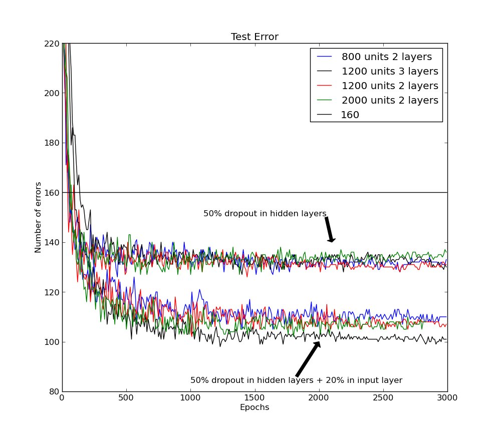
Fig. 1: The error rate on the MNIST test set for a variety of neural network architectures trained with backpropagation using 50% dropout for all hidden layers. The lower set of lines also use 20% dropout for the input layer. The best previously published result for this task using backpropagation without pre-training or weight-sharing or enhancements of the training set is shown as a horizontal line.

图 1：多种神经网络结构在反向传播训练下、所有隐层使用 50% dropout 时的 MNIST 测试错误率。下方一组曲线还对输入层使用 20% dropout。水平线表示此前用反向传播、无预训练、无权值共享、未增强训练集时该任务的最佳公开结果。

Dropout can also be combined with generative pre-training, but in this case we use a small learning rate and no weight constraints to avoid losing the feature detectors discovered by the pre-training. The publically available, pre-trained deep belief net described in [5] got 118 errors when it was fine-tuned using standard back-propagation and 92 errors when fine-tuned using 50% dropout of the hidden units. When the publically available code at URL was used to pre-train a deep Boltzmann machine five times, the unrolled network got 103, 97, 94, 93 and 88 errors when fine-tuned using standard backpropagation and 83, 79, 78, 78 and 77 errors when using 50% dropout of the hidden units. The mean of 79 errors is a record for methods that do not use prior knowledge or enhanced training sets (For details see Appendix A).

Dropout 也可与生成式预训练结合；此时我们用较小学习率且不加权重约束，以免丢掉预训练发现的特征检测器。文献 [5] 中公开可用的预训练深度信念网，用标准反向传播微调得 118 个错误，隐单元 50% dropout 微调得 92 个错误。用公开代码预训练深度玻尔兹曼机五次，展开网络用标准反向传播微调分别得 103、97、94、93、88 个错误，隐单元 50% dropout 则得 83、79、78、78、77；均值 79 个错误，是不使用先验知识或增强训练集的方法中的纪录（细节见附录 A）。

We then applied dropout to TIMIT, a widely used benchmark for recognition of clean speech with a small vocabulary. Speech recognition systems use hidden Markov models (HMMs) to deal with temporal variability and they need an acoustic model that determines how well a frame of coefficients extracted from the acoustic input fits each possible state of each hidden Markov model. Recently, deep, pre-trained, feedforward neural networks that map a short sequence of frames into a probability distribution over HMM states have been shown to outperform tradional Gaussian mixture models on both TIMIT [6] and a variety of more realistic large vocabulary tasks [7, 8].

接着我们把 dropout 用到 TIMIT——小词汇量干净语音识别的常用基准。语音识别系统用隐马尔可夫模型（HMM）处理时间可变性，并需要声学模型判断从声学输入抽出的一帧系数与各 HMM 各可能状态的匹配程度。近来，把短帧序列映射到 HMM 状态概率分布的深度预训练前馈神经网络，已在 TIMIT [6] 与多种更贴近现实的大词汇量任务 [7, 8] 上超过传统高斯混合模型。

Figure 2 shows the frame classification error rate on the core test set of the TIMIT benchmark when the central frame of a window is classified as belonging to the HMM state that is given the highest probability by the neural net. The input to the net is 21 adjacent frames with an advance of 10ms per frame. The neural net has 4 fully-connected hidden layers of 4000 units per layer and 185 “softmax” output units that are subsequently merged into the 39 distinct classes used for the benchmark. Dropout of 50% of the hidden units significantly improves classification for a variety of different network architectures (see figure 2). To get the frame recognition rate, the class probabilities that the neural network outputs for each frame are given to a decoder which knows about transition probabilities between HMM states and runs the Viterbi algorithm to infer the single best sequence of HMM states. Without dropout, the recognition rate is $22.7$% and with dropout this improves to $19.7$%, which is a record for methods that do not use any information about speaker identity.

图 2 给出 TIMIT 基准核心测试集上的帧 分类 错误率：窗口中心帧被标成神经网络赋予最高概率的那个 HMM 状态。网络输入为相邻 21 帧、每帧前进 10ms；网络有 4 个全连接隐层、每层 4000 单元，以及 185 个「softmax」输出单元，随后合并为基准所用的 39 个不同类别。对多种不同网络结构，隐单元 50% dropout 都显著改善分类（见图 2）。要得到帧 识别 率，把网络对每帧输出的类别概率交给了解 HMM 状态转移概率的解码器，用 Viterbi 算法推断单一最佳 HMM 状态序列。无 dropout 时识别率为 $22.7\%$，有 dropout 则提升到 $19.7\%$，是不使用说话人身份信息的方法中的纪录。

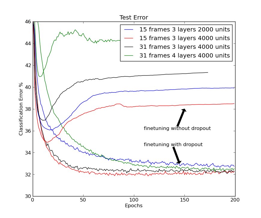
Fig. 2: The frame classification error rate on the core test set of the TIMIT benchmark. Comparison of standard and dropout finetuning for different network architectures. Dropout of 50% of the hidden units and 20% of the input units improves classification.

图 2：TIMIT 基准核心测试集上的帧 分类 错误率。比较不同网络结构下标准微调与 dropout 微调。隐单元 50% dropout、输入单元 20% dropout 可改善分类。

CIFAR-10 is a benchmark task for object recognition. It uses 32x32 downsampled color images of 10 different object classes that were found by searching the web for the names of the class (e.g. dog) or its subclasses (e.g. Golden Retriever). These images were labeled by hand to produce 50,000 training images and 10,000 test images in which there is a single dominant object that could plausibly be given the class name [9] (see figure 3). The best published error rate on the test set, without using transformed data, is 18.5% [10]. We achieved an error rate of 16.6% by using a neural network with three convolutional hidden layers interleaved with three “max-pooling” layers that report the maximum activity in local pools of convolutional units. These six layers were followed by one locally-connected layer (For details see Appendix D) . Using dropout in the last hidden layer gives an error rate of 15.6%.

CIFAR-10 是物体识别基准任务。它使用 10 个物体类的 32×32 降采样彩色图像；这些图像通过在网上搜索类名（如 dog）或其子类（如 Golden Retriever）得到，再人工标注，得到 50,000 张训练图像与 10,000 张测试图像，每张图有一个可合理赋予该类名的主导物体 [9]（见图 3）。不使用变换数据时，此前最佳公开测试错误率为 18.5% [10]。我们用三个卷积隐层与三个「最大池化」层交错、池化层报告卷积单元局部池中的最大活动，这六层后再接一个局部连接层（细节见附录 D），达到 16.6% 错误率。在最后隐层使用 dropout 则得到 15.6%。

Fig. 3: Ten examples of the class “bird” from the CIFAR-10 test set illustrating the variety of types of bird, viewpoint, lighting and background. The neural net gets all but the last two examples correct.

图 3：CIFAR-10 测试集中「鸟」类的十个例子，展示鸟种、视角、光照与背景的多样性。神经网络除最后两个例子外全部判对。

ImageNet is an extremely challenging object recognition dataset consisting of thousands of high-resolution images of thousands of classes of object [11]. In 2010, a subset of 1000 classes with roughly 1000 examples per class was the basis of an object recognition competition in which the winning entry, which was actually an average of six separate models, achieved an error rate of 47.2% on the test set. The current state-of-the-art result on this dataset is 45.7% [12]. We achieved comparable performance of 48.6% error using a single neural network with five convolutional hidden layers interleaved with “max-pooling” layer followed by two globally connected layers and a final 1000-way softmax layer. All layers had L2 weight constraints on the incoming weights of each hidden unit. Using 50% dropout in the sixth hidden layer reduces this to a record 42.4% (For details see Appendix E).

ImageNet 是极具挑战的物体识别数据集，包含数千类物体、数千张高分辨率图像 [11]。2010 年，约 1000 类、每类约 1000 例的子集成为物体识别竞赛基础；夺冠条目实际是六个独立模型的平均，测试错误率 47.2%。当时该数据集最优结果为 45.7% [12]。我们用单个神经网络达到可比较的 48.6%：五个卷积隐层与「最大池化」层交错，再接两个全局连接层与最终 1000 路 softmax。所有层对每个隐单元的入边权重施加 L2 约束。在第六隐层使用 50% dropout 后降到创纪录的 42.4%（细节见附录 E）。

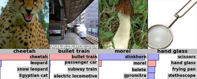
Fig. 4: Some Imagenet test cases with the probabilities of the best 5 labels underneath. Many of the top 5 labels are quite plausible.

图 4：若干 ImageNet 测试样例，下方给出最优 5 个标签的概率。许多 top-5 标签相当合理。

For the speech recognition dataset and both of the object recognition datasets it is necessary to make a large number of decisions in designing the architecture of the net. We made these decisions by holding out a separate validation set that was used to evaluate the performance of a large number of different architectures and we then used the architecture that performed best with dropout on the validation set to assess the performance of dropout on the real test set.

对语音识别数据集以及两个物体识别数据集，设计网络结构时需做大量决策。我们通过留出单独验证集评估大量不同结构的表现来做这些决策，再用在验证集上配合 dropout 表现最好的结构，评估 dropout 在真实测试集上的表现。

The Reuters dataset contains documents that have been labeled with a hierarchy of classes. We created training and test sets each containing 201,369 documents from 50 mutually exclusive classes. Each document was represented by a vector of counts for 2000 common non-stop words, with each count $C$ being transformed to $\log(1+C)$. A feedforward neural network with 2 fully connected layers of 2000 hidden units trained with backpropagation gets 31.05% error on the test set. This is reduced to 29.62% by using 50% dropout (Appendix C).

Reuters 数据集包含按层次类别标注的文档。我们构造各含 201,369 篇文档、来自 50 个互斥类别的训练与测试集。每篇文档用 2000 个常见非停用词的计数向量表示，计数 $C$ 变换为 $\log(1+C)$。带 2 个全连接层、每层 2000 隐单元的前馈网络用反向传播训练，测试错误率 31.05%；使用 50% dropout 后降到 29.62%（附录 C）。

We have tried various dropout probabilities and almost all of them improve the generalization performance of the network. For fully connected layers, dropout in all hidden layers works better than dropout in only one hidden layer and more extreme probabilities tend to be worse, which is why we have used 0.5 throughout this paper. For the inputs, dropout can also help, though it it often better to retain more than 50% of the inputs. It is also possible to adapt the individual dropout probability of each hidden or input unit by comparing the average performance on a validation set with the average performance when the unit is present. This makes the method work slightly better. For datasets in which the required input-output mapping has a number of fairly different regimes, performance can probably be further improved by making the dropout probabilities be a learned function of the input, thus creating a statistically efficient “mixture of experts” [13] in which there are combinatorially many experts, but each parameter gets adapted on a large fraction of the training data.

我们尝试了多种 dropout 概率，几乎都能改善网络的泛化。对全连接层，所有隐层都 dropout 优于只在一个隐层 dropout；过于极端的概率往往更差，因此全文使用 0.5。对输入，dropout 也有帮助，但通常保留超过 50% 的输入更好。也可通过比较某单元在验证集上的平均表现与该单元存在时的平均表现，适配每个隐单元或输入单元各自的 dropout 概率，这会使方法略好一些。对所需输入—输出映射存在若干相当不同体制的数据集，或许还可把 dropout 概率学成输入的函数，从而构造统计上高效的「专家混合」[13]：专家组合数呈组合爆炸，但每个参数仍在训练数据的很大一部分上得到适配。

Dropout is considerably simpler to implement than Bayesian model averaging which weights each model by its posterior probability given the training data. For complicated model classes, like feedforward neural networks, Bayesian methods typically use a Markov chain Monte Carlo method to sample models from the posterior distribution [14]. By contrast, dropout with a probability of $0.5$ assumes that all the models will eventually be given equal importance in the combination but the learning of the shared weights takes this into account. At test time, the fact that the dropout decisions are independent for each unit makes it very easy to approximate the combined opinions of exponentially many dropout nets by using a single pass through the mean net. This is far more efficient than averaging the predictions of many separate models.

相比按训练数据后验概率加权各模型的贝叶斯模型平均，dropout 实现简单得多。对前馈神经网络这类复杂模型类，贝叶斯方法通常用马尔可夫链蒙特卡洛从后验分布采样模型 [14]。相比之下，概率为 $0.5$ 的 dropout 假设组合中所有模型最终同等重要，但共享权重的学习已把这一点考虑进去。测试时，各单元的 dropout 决策相互独立，使一次前向通过均值网络就能近似指数多个 dropout 网的综合意见。这比平均许多独立模型的预测高效得多。

A popular alternative to Bayesian model averaging is “bagging” in which different models are trained on different random selections of cases from the training set and all models are given equal weight in the combination [15]. Bagging is most often used with models such as decision trees because these are very quick to fit to data and very quick at test time[16]. Dropout allows a similar approach to be applied to feedforward neural networks which are much more powerful models. Dropout can be seen as an extreme form of bagging in which each model is trained on a single case and each parameter of the model is very strongly regularized by sharing it with the corresponding parameter in all the other models. This is a much better regularizer than the standard method of shrinking parameters towards zero.

贝叶斯模型平均的流行替代是「bagging」：在训练集的不同随机子集上训练不同模型，组合时各模型等权 [15]。Bagging 最常用于决策树等模型，因为它们拟合数据与测试时都很快 [16]。Dropout 使类似思路可用于强大得多的前馈神经网络。可把 dropout 看成极端形式的 bagging：每个模型只在单个样本上训练，且模型每个参数通过与所有其他模型中对应参数共享而受到极强正则。这比把参数往零收缩的标准方法是好得多的正则。

A familiar and extreme case of dropout is “naive bayes” in which each input feature is trained separately to predict the class label and then the predictive distributions of all the features are multiplied together at test time. When there is very little training data, this often works much better than logistic classification which trains each input feature to work well in the context of all the other features.

一个熟悉且极端的 dropout 情形是「朴素贝叶斯」：每个输入特征单独训练以预测类别标签，测试时再把所有特征的预测分布相乘。训练数据很少时，这往往远好于逻辑分类——后者训练每个输入特征在所有其他特征的上下文中表现良好。

Finally, there is an intriguing similarity between dropout and a recent theory of the role of sex in evolution [17]. One possible interpretation of the theory of mixability articulated in [17] is that sex breaks up sets of co-adapted genes and this means that achieving a function by using a large set of co-adapted genes is not nearly as robust as achieving the same function, perhaps less than optimally, in multiple alternative ways, each of which only uses a small number of co-adapted genes. This allows evolution to avoid dead-ends in which improvements in fitness require co- ordinated changes to a large number of co-adapted genes. It also reduces the probability that small changes in the environment will cause large decreases in fitness – a phenomenon which is known as “overfitting” in the field of machine learning.

最后，dropout 与近期关于性别在进化中作用的理论 [17] 有耐人寻味的相似。对 [17] 中阐述的可混合性理论，一种可能解读是：有性繁殖拆散共适应基因集合，这意味着用一大套共适应基因实现某功能，远不如用多种替代方式（或许并非最优）实现同一功能稳健——每种方式只使用少量共适应基因。这使进化避免死胡同：适应度提升需要对大量共适应基因做协同改变。它也降低环境小变化导致适应度大幅下降的概率——机器学习领域称之为「过拟合」。

References

参考文献

• 1. We thank N. Jaitly for help with TIMIT, H. Larochelle, R. Neal, K. Swersky and C.K.I. Williams for helpful discussions, and NSERC, Google and Microsoft Research for funding. GEH and RRS are members of the Canadian Institute for Advanced Research.

• 1. 感谢 N. Jaitly 在 TIMIT 上的帮助，H. Larochelle、R. Neal、K. Swersky 与 C.K.I. Williams 的有益讨论，以及 NSERC、Google 与 Microsoft Research 的资助。GEH 与 RRS 是加拿大高级研究院成员。

[1] D. E. Rumelhart, G. E. Hinton, R. J. Williams, Nature 323 , 533 (1986).

[2] G. E. Hinton, Neural Computation 14 , 1771 (2002).

[3] L. M. G. D. C. Ciresan, U. Meier, J. Schmidhuber, Neural Computation 22 , 3207 (2010).

[4] Y. B. Y. Lecun, L. Bottou, P. Haffner, Proceedings of the IEEE 86 , 2278 (1998).

[5] G. E. Hinton, R. Salakhutdinov, Science 313 , 504 (2006).

[6] A. Mohamed, G. Dahl, G. Hinton, IEEE Transactions on Audio, Speech, and Language Processing, 20 , 14 (2012).

[7] G. Dahl, D. Yu, L. Deng, A. Acero, IEEE Transactions on Audio, Speech, and Language Processing, 20 , 30 (2012).

[8] N. Jaitly, P. Nguyen, A. Senior, V. Vanhoucke, An Application OF Pretrained Deep Neural Networks To Large Vocabulary Conversational Speech Recognition, Tech. Rep. 001 , Department of Computer Science, University of Toronto (2012).

[9] A. Krizhevsky, Learning multiple layers of features from tiny images, Tech. Rep. 001 , Department of Computer Science, University of Toronto (2009).

[10] A. Coates, A. Y. Ng, ICML (2011), pp. 921–928.

[11] J. Deng, et al. , CVPR09 (2009).

[12] J. Sanchez, F. Perronnin, CVPR11 (2011).

[13] S. J. N. R. A. Jacobs, M. I. Jordan, G. E. Hinton, Neural Computation 3 , 79 (1991).

[14] R. M. Neal, Bayesian Learning for Neural Networks, Lecture Notes in Statistics No. 118 (Springer-Verlag, New York, 1996).

[15] L. Breiman, Machine Learning 24 , 123 (1996).

[16] L. Breiman, Machine Learning 45 , 5 (2001).

[17] J. D. A. Livnat, C. Papadimitriou, M. W. Feldman, PNAS 105 , 19803– (2008).

[18] R. R. Salakhutdinov, G. E. Hinton, Artificial Intelligence and Statistics (2009).

[19] D. D. Lewis, T. G. R. Y. Yang, Journal of Machine Learning 5 , 361 (2004).

Appendix A Experiments on MNIST

附录 A MNIST 实验

A.1 Details for dropout training

A.1 Dropout 训练细节

The MNIST dataset consists of 28 $\times$ 28 digit images - 60,000 for training and 10,000 for testing. The objective is to classify the digit images into their correct digit class. We experimented with neural nets of different architectures (different number of hidden units and layers) to evaluate the sensitivity of the dropout method to these choices. We show results for 4 nets (784-800-800-10, 784-1200-1200-10, 784-2000-2000-10, 784-1200-1200-1200-10). For each of these architectures we use the same dropout rates - 50% dropout for all hidden units and 20% dropout for visible units. We use stochastic gradient descent with 100-sized minibatches and a cross-entropy objective function. An exponentially decaying learning rate is used that starts at the value of 10.0 (applied to the average gradient in each minibatch). The learning rate is multiplied by 0.998 after each epoch of training. The incoming weight vector corresponding to each hidden unit is constrained to have a maximum squared length of $l$. If, as a result of an update, the squared length exceeds $l$, the vector is scaled down so as to make it have a squared length of $l$. Using cross validation we found that $l=15$ gave best results. Weights are initialzed to small random values drawn from a zero-mean normal distribution with standard deviation 0.01. Momentum is used to speed up learning. The momentum starts off at a value of 0.5 and is increased linearly to 0.99 over the first 500 epochs, after which it stays at 0.99. Also, the learning rate is multiplied by a factor of (1-momentum). No weight decay is used. Weights were updated at the end of each minibatch. Training was done for 3000 epochs. The weight update takes the following form:

MNIST 数据集由 28 $\times$ 28 数字图像组成——60,000 张训练、10,000 张测试。目标是把数字图像分到正确数字类别。我们试验不同结构（不同隐单元数与层数）的神经网络，以评估 dropout 方法对这些选择的敏感性。展示 4 个网络的结果（784-800-800-10、784-1200-1200-10、784-2000-2000-10、784-1200-1200-1200-10）。对各结构使用相同 dropout 率——所有隐单元 50%、可见单元 20%。用批量大小 100 的随机梯度下降与交叉熵目标。学习率指数衰减，初值 10.0（作用于每个小批量的平均梯度），每轮训练后乘以 0.998。每个隐单元对应的入边权重向量约束最大平方长度为 $l$；若更新后平方长度超过 $l$，则缩放使平方长度回到 $l$。交叉验证发现 $l=15$ 最好。权重初始化为零均值、标准差 0.01 的正态小随机值。用动量加速学习：动量从 0.5 起步，前 500 轮线性增至 0.99，之后保持 0.99。学习率还乘以 (1-momentum)。不使用权重衰减。每个小批量结束时更新权重。共训练 3000 轮。权重更新形式为：

$$\displaystyle\Delta w^{t} \\ \displaystyle= \\ \displaystyle p^{t}\Delta w^{t-1}-(1-p^{t})\epsilon^{t}\langle\nabla_{w}L\rangle \\ \displaystyle w^{t} \\ \displaystyle= \\ \displaystyle w^{t-1}+\Delta w^{t},$$

where,

其中，

$$\displaystyle\epsilon^{t} \ \displaystyle= \ \displaystyle\epsilon_{0}f^{t} \ \displaystyle p^{t} \ \displaystyle= \ \displaystyle\begin{cases}\frac{t}{T}p_{i}+(1-\frac{t}{T})p_{f}&t<T\
p_{f}&t\geq T\end{cases}$$

with $\epsilon_{0}=10.0$, $f=0.998$, $p_{i}=0.5$, $p_{f}=0.99$, $T=500$. While using a constant learning rate also gives improvements over standard backpropagation, starting with a high learning rate and decaying it provided a significant boost in performance. Constraining input vectors to have a fixed length prevents weights from increasing arbitrarily in magnitude irrespective of the learning rate. This gives the network a lot of opportunity to search for a good configuration in the weight space. As the learning rate decays, the algorithm is able to take smaller steps and finds the right step size at which it can make learning progress. Using a high final momentum distributes gradient information over a large number of updates making learning stable in this scenario where each gradient computation is for a different stochastic network.

取 $\epsilon_{0}=10.0$，$f=0.998$，$p_{i}=0.5$，$p_{f}=0.99$，$T=500$。恒定学习率也优于标准反向传播，但从高学习率起步再衰减能显著再抬表现。把入边向量约束到固定长度，使权重幅度不会随学习率任意增大。这给网络大量机会在权重空间中搜索好配置。学习率衰减后，算法可迈更小步，并找到能推进学习的合适步长。高终值动量把梯度信息分散到大量更新上，使每个梯度对应不同随机网络时学习仍稳定。

A.2 Details for dropout finetuning

A.2 Dropout 微调细节

Apart from training a neural network starting from random weights, dropout can also be used to finetune pretrained models. We found that finetuning a model using dropout with a small learning rate can give much better performace than standard backpropagation finetuning.

除从随机权重起步训练外，dropout 也可用于微调预训练模型。我们发现用小学习率做 dropout 微调，可比标准反向传播微调好得多。

Deep Belief Nets - We took a neural network pretrained using a Deep Belief Network [5]. It had a 784-500-500-2000 architecture and was trained using greedy layer-wise Contrastive Divergence learning [^1]. Instead of fine-tuning it with the usual backpropagation algorithm, we used the dropout version of it. Dropout rate was same as before : 50% for hidden units and 20% for visible units. A constant small learning rate of 1.0 was used. No constraint was imposed on the length of incoming weight vectors. No weight decay was used. All other hyper-parameters were set to be the same as before. The model was trained for 1000 epochs with stochstic gradient descent using minibatches of size 100. While standard back propagation gave about 118 errors, dropout decreased the errors to about 92.

深度信念网 — 我们取用深度信念网预训练的神经网络 [5]。结构为 784-500-500-2000，用贪心逐层对比散度学习训练。[^1] 不用常规反向传播微调，而用其 dropout 版本。Dropout 率同前：隐单元 50%、可见单元 20%。使用恒定小学习率 1.0。不对入边权重向量长度施加约束。不使用权重衰减。其余超参同前。用批量大小 100 的随机梯度下降训练 1000 轮。标准反向传播约 118 个错误，dropout 降到约 92。

Deep Boltzmann Machines - We also took a pretrained Deep Boltzmann Machine [18] [^2] (784-500-1000-10) and finetuned it using dropout-backpropagation. The model uses a 1784 - 500 - 1000 - 10 architecture (The extra 1000 input units come from the mean-field activations of the second layer of hidden units in the DBM, See [18] for details). All finetuning hyper-parameters were set to be the same as the ones used for a Deep Belief Network. We were able to get a mean of about 79 errors with dropout whereas usual finetuning gives about 94 errors.

深度玻尔兹曼机 — 我们还取预训练的深度玻尔兹曼机 [18] [^2]（784-500-1000-10），用 dropout-反向传播微调。模型使用 1784-500-1000-10 结构（额外 1000 个输入单元来自 DBM 第二隐层的平均场激活，细节见 [18]）。全部微调超参与深度信念网相同。Dropout 平均约 79 个错误，常规微调约 94。

(a)

A.3 Effect on features

A.3 对特征的影响

One reason why dropout gives major improvements over backpropagation is that it encourages each individual hidden unit to learn a useful feature without relying on specific other hidden units to correct its mistakes. In order to verify this and better understand the effect of dropout on feature learning, we look at the first level of features learned by a 784-500-500 neural network without any generative pre-training. The features are shown in Figure 5. Each panel shows 100 random features learned by each network. The features that dropout learns are simpler and look like strokes, whereas the ones learned by standard backpropagation are difficult to interpret. This confirms that dropout indeed forces the discriminative model to learn good features which are less co-adapted and leads to better generalization.

Dropout 相对反向传播大幅提升的一个原因是：它促使每个隐单元独自学会有用特征，而不依赖特定其他隐单元来纠正其错误。为验证这一点并更好理解 dropout 对特征学习的影响，我们查看无生成式预训练的 784-500-500 网络所学的第一层特征，见图 5。每块面板展示各网络学到的 100 个随机特征。Dropout 学到的特征更简单，看起来像笔划；标准反向传播学到的则难以解释。这证实 dropout 确实迫使判别模型学习更少共适应的好特征，从而更好泛化。

Appendix B Experiments on TIMIT

附录 B TIMIT 实验

The TIMIT Acoustic-Phonetic Continuous Speech Corpus is a standard dataset used for evaluation of automatic speech recognition systems. It consists of recordings of 630 speakers of 8 dialects of American English each reading 10 phonetically-rich sentences. It also comes with the word and phone-level transcriptions of the speech. The objective is to convert a given speech signal into a transcription sequence of phones. This data needs to be pre-processed to extract input features and output targets. We used Kaldi, an open source code library for speech [^3], to pre-process the dataset so that our results can be reproduced exactly. The inputs to our networks are log filter bank responses. They are extracted for 25 ms speech windows with strides of 10 ms.

TIMIT 声学—音素连续语音语料是自动语音识别系统评估的标准数据集。它包含 630 名、涵盖 8 种美式英语方言的说话人录音，每人朗读 10 句富含音素的句子，并附带词级与音素级转写。目标是把给定语音信号转成音素转写序列。数据需预处理以抽取输入特征与输出目标。我们用开源语音库 Kaldi [^3] 做预处理，以便结果可精确复现。网络输入为对数滤波器组响应，按 25 ms 语音窗、步长 10 ms 抽取。

Each dimension of the input representation was normalized to have mean 0 and variance 1. Minibatches of size 100 were used for both pretraining and dropout finetuning. We tried several network architectures by varying the number of input frames (15 and 31), number of layers in the neural network (3, 4 and 5) and the number of hidden units in each layer (2000 and 4000). Figure 6 shows the validation error curves for a number of these combinations. Using dropout consistently leads to lower error rates.

输入表示的每一维归一化到均值 0、方差 1。预训练与 dropout 微调均用批量大小 100。我们通过改变输入帧数（15 与 31）、网络层数（3、4、5）以及每层隐单元数（2000 与 4000）试验多种结构。图 6 给出若干组合的验证错误率曲线。使用 dropout 一致带来更低错误率。

(a)

B.1 Pretraining

B.1 预训练

For all our experiments on TIMIT, we pretrain the neural network with a Deep Belief Network [5]. Since the inputs are real-valued, the first layer was pre-trained as a Gaussian RBM. Visible biases were initialized to zero and weights to random numbers sampled from a zero-mean normal distribution with standard deviation 0.01. The variance of each visible unit was set to 1.0 and not learned. Learning was done by minimizing Contrastive Divergence. Momentum was used to speed up learning. Momentum started at 0.5 and was increased linearly to 0.9 over 20 epochs. A learning rate of 0.001 on the average gradient was used (which was then multiplied by 1-momentum). An L2 weight decay of 0.001 was used. The model was trained for 100 epochs.

对所有 TIMIT 实验，我们用深度信念网 [5] 预训练神经网络。因输入为实值，第一层预训练为高斯 RBM。可见偏置初始化为零，权重从零均值、标准差 0.01 的正态采样。每个可见单元方差固定为 1.0 且不学习。学习通过最小化对比散度完成。用动量加速：动量从 0.5 起步，20 轮内线性增至 0.9。平均梯度上的学习率为 0.001（再乘以 1-momentum）。L2 权重衰减 0.001。模型训练 100 轮。

All subsequent layers were trained as binary RBMs. A learning rate of 0.01 was used. The visible bias of each unit was initialized to $\log(p/(1-p))$ where $p$ was the mean activation of that unit in the dataset. All other hyper-parameters were set to be the same as those we used for the Gaussian RBM. Each layer was trained for 50 epochs.

后续各层训练为二值 RBM。学习率 0.01。每个单元的可见偏置初始化为 $\log(p/(1-p))$，其中 $p$ 为该单元在数据集中的平均激活。其余超参与高斯 RBM 相同。每层训练 50 轮。

B.2 Dropout Finetuning

B.2 Dropout 微调

The pretrained RBMs were used to initialize the weights in a neural network. The network was then finetuned with dropout-backpropagation. Momentum was increased from 0.5 to 0.9 linearly over 10 epochs. A small constant learning rate of 1.0 was used (applied to the average gradient on a minibatch). All other hyperparameters are the same as for MNIST dropout finetuning. The model needs to be run for about 200 epochs to converge. The same network was also finetuned with standard backpropagation using a smaller learning rate of 0.1, keeping all other hyperparameters

预训练的 RBM 用于初始化神经网络权重。随后用 dropout-反向传播微调。动量在 10 轮内从 0.5 线性增至 0.9。使用恒定小学习率 1.0（作用于小批量平均梯度）。其余超参与 MNIST dropout 微调相同。模型约需 200 轮收敛。同一网络也用标准反向传播微调，学习率更小为 0.1，其余超参保持不变。

Figure 6 shows the frame classification error and cross-entropy objective value on the training and validation sets. We compare the performance of dropout and standard backpropagation on several network architectures and input representations. Dropout consistently achieves lower error and cross-entropy. It significantly controls overfitting, making the method robust to choices of network architecture. It allows much larger nets to be trained and removes the need for early stopping. We also observed that the final error obtained by the model is not very sensitive to the choice of learning rate and momentum.

图 6 给出训练集与验证集上的帧分类错误率与交叉熵目标值。我们在多种网络结构与输入表示上比较 dropout 与标准反向传播。Dropout 一致取得更低错误与交叉熵。它显著控制过拟合，使方法对网络结构选择更稳健；允许训练大得多的网络，并去掉对早停的依赖。我们还观察到，模型最终错误对学习率与动量的选择不太敏感。

Appendix C Experiments on Reuters

附录 C Reuters 实验

Reuters Corpus Volume I (RCV1-v2) [19] is an archive of 804,414 newswire stories that have been manually categorized into 103 topics[^4]. The corpus covers four major groups: corporate/industrial, economics, government/social, and markets. Sample topics include Energy Markets, Accounts/Earnings, Government Borrowings, Disasters and Accidents, Interbank Markets, Legal/Judicial, Production/Services, etc. The topic classes form a tree which is typically of depth three.

Reuters Corpus Volume I（RCV1-v2）[19] 是含 804,414 篇新闻电讯的档案，人工分为 103 个主题。[^4] 语料覆盖四大组：公司/工业、经济、政府/社会与市场。示例主题包括能源市场、账目/收益、政府借款、灾害事故、同业拆借市场、法律/司法、生产/服务等。主题类别构成通常深度为三的树。

We took the dataset and split it into 63 classes based on the the 63 categories at the second-level of the category tree. We removed 11 categories that did not have any data and one category that had only 4 training examples. We also removed one category that covered a huge chunk (25%) of the examples. This left us with 50 classes and 402,738 documents. We divided the documents into equal-sized training and test sets randomly. Each document was represented using the 2000 most frequent non-stopwords in the dataset.

我们按类别树第二层的 63 个类别把数据分成 63 类。去掉 11 个无数据的类别、1 个仅有 4 个训练例的类别，以及覆盖约 25% 样本的 1 个大类。剩下 50 类、402,738 篇文档。随机均分为等大的训练与测试集。每篇文档用数据集中最常见的 2000 个非停用词表示。

(a)

We trained a neural network using dropout-backpropagation and compared it with standard backpropagation. We used a 2000-2000-1000-50 architecture. The training hyperparameters are same as that in MNIST dropout training (Appendix A.1). Training was done for 500 epochs.

我们用 dropout-反向传播训练神经网络，并与标准反向传播比较。结构为 2000-2000-1000-50。训练超参与 MNIST dropout 训练（附录 A.1）相同。共训练 500 轮。

Figure 7 shows the training and test set errors as learning progresses. We show two nets - one with a 2000-2000-1000-50 and another with a 2000-1000-1000-50 architecture trained with and without dropout. As in all previous datasets discussed so far, we obtain significant improvements here too. The learning not only results in better generalization, but also proceeds smoothly, without the need for early stopping.

图 7 给出学习过程中训练与测试错误。展示两个网络——2000-2000-1000-50 与 2000-1000-1000-50——分别有无 dropout 的训练。与此前所有数据集一样，这里也有显著提升。学习不仅泛化更好，而且过程平稳，无需早停。

Appendix D Tiny Images and CIFAR-10

附录 D Tiny Images 与 CIFAR-10

The Tiny Images dataset contains 80 million $32\times 32$ color images collected from the web. The images were found by searching various image search engines for English nouns, so each image comes with a very unreliable label, which is the noun that was used to find it. The CIFAR-10 dataset is a subset of the Tiny Images dataset which contains 60000 images divided among ten classes[^5]. Each class contains 5000 training images and 1000 testing images. The classes are airplane, automobile, bird, cat, deer, dog, frog, horse, ship, and truck. The CIFAR-10 dataset was obtained by filtering the Tiny Images dataset to remove images with incorrect labels. The CIFAR-10 images are highly varied, and there is no canonical viewpoint or scale at which the objects appear. The only criteria for including an image were that the image contain one dominant instance of a CIFAR-10 class, and that the object in the image be easily identifiable as belonging to the class indicated by the image label.

Tiny Images 数据集含从网上收集的 8000 万张 $32\times 32$ 彩色图像。图像通过在各图像搜索引擎搜索英语名词得到，因此每张图带有很不可靠的标签——即用来找到它的那个名词。CIFAR-10 是 Tiny Images 的子集，含 60000 张图像、分为十类。[^5] 每类 5000 张训练、1000 张测试。类别为 airplane、automobile、bird、cat、deer、dog、frog、horse、ship 与 truck。CIFAR-10 通过对 Tiny Images 过滤去掉错误标签得到。图像高度多样，物体没有规范视角或尺度。纳入图像的唯一标准是：图中含 CIFAR-10 某类的一个主导实例，且物体易于识别为标签所示类别。

Appendix E ImageNet

附录 E ImageNet

ImageNet is a dataset of millions of labeled images in thousands of categories. The images were collected from the web and labelled by human labellers using Amazon’s Mechanical Turk crowd-sourcing tool. In 2010, a subset of roughly 1000 images in each of 1000 classes was the basis of an object recognition competition, a part of the Pascal Visual Object Challenge. This is the version of ImageNet on which we performed our experiments. In all, there are roughly 1.3 million training images, 50000 validation images, and 150000 testing images. This dataset is similar in spirit to the CIFAR-10, but on a much bigger scale. The images are full-resolution, and there are 1000 categories instead of ten. Another difference is that the ImageNet images often contain multiple instances of ImageNet objects, simply due to the sheer number of object classes. For this reason, even a human would have difficulty approaching perfect accuracy on this dataset. For our experiments we resized all images to $256\times 256$ pixels.

ImageNet 是含数百万标注图像、数千类别的数据集。图像从网上收集，并由 Amazon Mechanical Turk 众包人工标注。2010 年，约 1000 类、每类约 1000 张图像的子集成为物体识别竞赛（Pascal Visual Object Challenge 的一部分）的基础。我们的实验即在该版 ImageNet 上进行。总计约 130 万训练图像、50000 验证、150000 测试。精神上类似 CIFAR-10，但规模大得多：图像为全分辨率，类别为 1000 而非十。另一差异是 ImageNet 图像常含多个 ImageNet 物体实例，只因物体类极多。因此即使人类也难以逼近完美准确率。实验中我们把所有图像缩放到 $256\times 256$ 像素。

Appendix F Convolutional Neural Networks

附录 F 卷积神经网络

Our models for CIFAR-10 and ImageNet are deep, feed-forward convolutional neural networks (CNNs). Feed-forward neural networks are models which consist of several layers of “neurons”, where each neuron in a given layer applies a linear filter to the outputs of the neurons in the previous layer. Typically, a scalar bias is added to the filter output and a nonlinear activation function is applied to the result before the neuron’s output is passed to the next layer. The linear filters and biases are referred to as weights, and these are the parameters of the network that are learned from the training data.

我们用于 CIFAR-10 与 ImageNet 的模型是深度前馈卷积神经网络（CNN）。前馈神经网络由多层「神经元」组成，给定层中每个神经元对上一层神经元输出施加线性滤波。通常在滤波输出上加标量偏置，再经非线性激活后传给下一层。线性滤波器与偏置称为 权重，是从训练数据学习的网络参数。

CNNs differ from ordinary neural networks in several ways. First, neurons in a CNN are organized topographically into a bank that reflects the organization of dimensions in the input data. So for images, the neurons are laid out on a 2D grid. Second, neurons in a CNN apply filters which are local in extent and which are centered at the neuron’s location in the topographic organization. This is reasonable for datasets where we expect the dependence of input dimensions to be a decreasing function of distance, which is the case for pixels in natural images. In particular, we expect that useful clues to the identity of the object in an input image can be found by examining small local neighborhoods of the image. Third, all neurons in a bank apply the same filter, but as just mentioned, they apply it at different locations in the input image. This is reasonable for datasets with roughly stationary statistics, such as natural images. We expect that the same kinds of structures can appear at all positions in an input image, so it is reasonable to treat all positions equally by filtering them in the same way. In this way, a bank of neurons in a CNN applies a convolution operation to its input. A single layer in a CNN typically has multiple banks of neurons, each performing a convolution with a different filter. These banks of neurons become distinct input channels into the next layer. The distance, in pixels, between the boundaries of the receptive fields of neighboring neurons in a convolutional bank determines the stride with which the convolution operation is applied. Larger strides imply fewer neurons per bank. Our models use a stride of one pixel unless otherwise noted.

CNN 与普通神经网络有若干不同。第一，CNN 中的神经元按地形学组织成反映输入数据维度组织的组（bank）。对图像而言，神经元排布在二维网格上。第二，CNN 中的神经元施加局部范围的滤波器，并以该神经元在地形组织中的位置为中心。这对我们期望输入维度依赖随距离递减的数据集是合理的——自然图像的像素正是如此。尤其是，识别输入图像中物体身份的有用线索，往往可通过查看图像的小局部邻域得到。第三，同一 bank 中所有神经元施加相同滤波器，但如上所述作用于输入图像的不同位置。这对统计大致平稳的数据集（如自然图像）合理：我们期望同类结构可出现在输入图像任意位置，因此以相同方式滤波、平等对待各位置是合理的。于是 CNN 中一个 bank 对其输入施加卷积。CNN 的单层通常有多个 bank，各自用不同滤波器做卷积；这些 bank 成为下一层的不同输入通道。卷积 bank 中相邻神经元感受野边界之间的像素距离，决定卷积操作的 步幅。更大步幅意味着每个 bank 神经元更少。除非另有说明，我们的模型使用 1 像素步幅。

One important consequence of this convolutional shared-filter architecture is a drastic reduction in the number of parameters relative to a neural net in which all neurons apply different filters. This reduces the net’s representational capacity, but it also reduces its capacity to overfit, so dropout is far less advantageous in convolutional layers.

这种卷积共享滤波器结构的一个重要后果是：相对每个神经元使用不同滤波器的网络，参数量大幅减少。这降低网络的表示容量，也降低过拟合容量，因此 dropout 在卷积层上远不那么有利。

F.1 Pooling

F.1 池化

CNNs typically also feature “pooling” layers which summarize the activities of local patches of neurons in convolutional layers. Essentially, a pooling layer takes as input the output of a convolutional layer and subsamples it. A pooling layer consists of pooling units which are laid out topographically and connected to a local neighborhood of convolutional unit outputs from the same bank. Each pooling unit then computes some function of the bank’s output in that neighborhood. Typical functions are maximum and average. Pooling layers with such units are called max-pooling and average-pooling layers, respectively. The pooling units are usually spaced at least several pixels apart, so that there are fewer total pooling units than there are convolutional unit outputs in the previous layer. Making this spacing smaller than the size of the neighborhood that the pooling units summarize produces overlapping pooling. This variant makes the pooling layer produce a coarse coding of the convolutional unit outputs, which we have found to aid generalization in our experiments. We refer to this spacing as the stride between pooling units, analogously to the stride between convolutional units. Pooling layers introduce a level of local translation invariance to the network, which improves generalization. They are the analogues of complex cells in the mammalian visual cortex, which pool activities of multiple simple cells. These cells are known to exhibit similar phase-invariance properties.

CNN 通常还有「池化」层，用于汇总卷积层中局部片上的神经元活动。本质上，池化层以卷积层输出为输入并对其子采样。池化层由按地形排布的池化单元组成，每个单元连接到同一 bank 中卷积单元输出的局部邻域，再对该邻域计算某种函数。典型函数是最大值与平均值，对应最大池化与平均池化层。池化单元通常至少间隔若干像素，使总数少于上一层卷积输出。若该间隔小于池化单元所汇总的邻域大小，则产生 重叠池化。这一变体使池化层对卷积输出做粗编码，我们在实验中发现有助于泛化。我们把该间隔称为池化单元之间的 步幅，类比卷积单元步幅。池化层为网络引入局部平移不变性，改善泛化。它们类似于哺乳动物视皮层中的 复杂细胞，后者汇总多个简单细胞的活动，并已知表现出类似的相位不变性。

F.2 Local response normalization

F.2 局部响应归一化

Our networks also include response normalization layers. This type of layer encourages competition for large activations among neurons belonging to different banks. In particular, the activity $a_{x,y}^{i}$ of a neuron in bank $i$ at position $(x,y)$ in the topographic organization is divided by

我们的网络还包含响应归一化层。这类层鼓励不同 bank 的神经元竞争大激活。具体地，bank $i$ 中位于地形组织位置 $(x,y)$ 的神经元活动 $a_{x,y}^{i}$ 被除以

$$\left(1+\alpha\sum_{j=i-N/2}^{i+N/2}(a_{x,y}^{j})^{2}\right)^{\beta}$$

where the sum runs over $N$ “adjacent” banks of neurons at the same position in the topographic organization. The ordering of the banks is of course arbitrary and determined before training begins. Response normalization layers implement a form of lateral inhibition found in real neurons. The constants $N,\alpha$, and $\beta$ are hyper-parameters whose values are determined using a validation set.

其中求和遍历在地形组织 同一位置 上 $N$ 个「相邻」神经元 bank。Bank 的排序当然是任意的，并在训练开始前确定。响应归一化层实现真实神经元中可见的一种侧抑制。常数 $N$、$\alpha$ 与 $\beta$ 是超参，取值由验证集确定。

F.3 Neuron nonlinearities

F.3 神经元非线性

All of the neurons in our networks utilize the max-with-zero nonlinearity. That is, their output is computed as $a_{x,y}^{i}=\max(0,z_{x,y}^{i})$ where $z_{x,y}^{i}$ is the total input to the neuron (equivalently, the output of the neuron’s linear filter added to the bias). This nonlinearity has several advantages over traditional saturating neuron models, including a significant reduction in the training time required to reach a given error rate. This nonlinearity also reduces the need for contrast-normalization and similar data pre-processing schemes, because neurons with this nonlinearity do not saturate – their activities simply scale up when presented with unusually large input values. Consequently, the only data pre-processing step which we take is to subtract the mean activity from each pixel, so that the data is centered. So we train our networks on the (centered) raw RGB values of the pixels.

我们网络中所有神经元使用 max-with-zero 非线性。亦即输出为 $a_{x,y}^{i}=\max(0,z_{x,y}^{i})$，其中 $z_{x,y}^{i}$ 是神经元总输入（等价于线性滤波输出加偏置）。相对传统饱和神经元模型，该非线性有若干优点，包括达到给定错误率所需训练时间显著缩短。它也减少对对比度归一化等数据预处理的依赖——因为这类神经元不饱和：输入异常大时活动只是按比例放大。因此我们唯一的预处理是从每个像素减去平均活动，使数据居中。于是网络在（居中后的）原始 RGB 像素值上训练。

F.4 Objective function

F.4 目标函数

Our networks maximize the multinomial logistic regression objective, which is equivalent to minimizing the average across training cases of the cross-entropy between the true label distribution and the model’s predicted label distribution.

我们的网络最大化多项式逻辑回归目标，等价于最小化训练样本上真实标签分布与模型预测标签分布之间交叉熵的平均。

F.5 Weight initialization

F.5 权重初始化

We initialize the weights in our model from a zero-mean normal distribution with a variance set high enough to produce positive inputs into the neurons in each layer. This is a slightly tricky point when using the max-with-zero nonlinearity. If the input to a neuron is always negative, no learning will take place because its output will be uniformly zero, as will the derivative of its output with respect to its input. Therefore it’s important to initialize the weights from a distribution with a sufficiently large variance such that all neurons are likely to get positive inputs at least occasionally. In practice, we simply try different variances until we find an initialization that works. It usually only takes a few attempts. We also find that initializing the biases of the neurons in the hidden layers with some positive constant (1 in our case) helps get learning off the ground, for the same reason.

模型权重从零均值正态分布初始化，方差设得足够高，使每层神经元能得到正输入。使用 max-with-zero 非线性时这一点略棘手。若某神经元输入恒为负，则输出恒为零，输出对输入的导数亦为零，学习不会发生。因此重要的是从方差足够大的分布初始化，使所有神经元至少偶尔得到正输入。实践中我们只是尝试不同方差直到找到可用初始化，通常只需几次。我们还发现把隐层神经元偏置初始化为某个正常数（本文取 1）有助于启动学习，原因相同。

F.6 Training

F.6 训练

We train our models using stochastic gradient descent with a batch size of 128 examples and momentum of 0.9. Therefore the update rule for weight $w$ is

我们用批量大小 128、动量 0.9 的随机梯度下降训练模型。因此权重 $w$ 的更新规则为

$$\displaystyle v_{i+1} \\ \displaystyle= \\ \displaystyle 0.9v_{i}+\epsilon<\frac{\partial E}{\partial w_{i}}>_{i} \\ \displaystyle w_{i+1} \\ \displaystyle= \\ \displaystyle w_{i}+v_{i+1}$$

where $i$ is the iteration index, $v$ is a momentum variable, $\epsilon$ is the learning rate, and $<\frac{\partial E}{\partial w_{i}}>_{i}$ is the average over the $i^{th}$ batch of the derivative of the objective with respect to $w_{i}$. We use the publicly available cuda-convnet package to train all of our models on a single NVIDIA GTX 580 GPU. Training on CIFAR-10 takes roughly 90 minutes. Training on ImageNet takes roughly four days with dropout and two days without.

其中 $i$ 为迭代索引，$v$ 为动量变量，$\epsilon$ 为学习率，$<\frac{\partial E}{\partial w_{i}}>_{i}$ 为第 $i$ 个批量上目标对 $w_{i}$ 导数的平均。我们用公开的 cuda-convnet 包在单块 NVIDIA GTX 580 GPU 上训练全部模型。CIFAR-10 训练约 90 分钟；ImageNet 有 dropout 约四天，无 dropout 约两天。

F.7 Learning rates

F.7 学习率

We use an equal learning rate for each layer, whose value we determine heuristically as the largest power of ten that produces reductions in the objective function. In practice it is typically of the order $10^{-2}$ or $10^{-3}$. We reduce the learning rate twice by a factor of ten shortly before terminating training.

各层使用相同学习率，取值启发式取能使目标下降的最大十的幂。实践中通常量级为 $10^{-2}$ 或 $10^{-3}$。终止训练前不久，我们两次把学习率缩小十倍。

Appendix G Models for CIFAR-10

附录 G CIFAR-10 模型

Our model for CIFAR-10 without dropout is a CNN with three convolutional layers. Pooling layers follow all three. All of the pooling layers summarize a $3\times 3$ neighborhood and use a stride of 2. The pooling layer which follows the first convolutional layer performs max-pooling, while the remaining pooling layers perform average-pooling. Response normalization layers follow the first two pooling layers, with $N=9$, $\alpha=0.001$, and $\beta=0.75$. The upper-most pooling layer is connected to a ten-unit softmax layer which outputs a probability distribution over class labels. All convolutional layers have 64 filter banks and use a filter size of $5\times 5$ (times the number of channels in the preceding layer).

无 dropout 的 CIFAR-10 模型是含三个卷积层的 CNN。三层后均接池化层。所有池化层汇总 $3\times 3$ 邻域、步幅为 2。第一卷积层后的池化做最大池化，其余做平均池化。前两个池化层后接响应归一化，$N=9$，$\alpha=0.001$，$\beta=0.75$。最上层池化连接到十单元 softmax，输出类别标签概率分布。所有卷积层有 64 个滤波器 bank，滤波器大小 $5\times 5$（再乘以上一层通道数）。

Our model for CIFAR-10 with dropout is similar, but because dropout imposes a strong regularization on the network, we are able to use more parameters. Therefore we add a fourth weight layer, which takes its input from the third pooling layer. This weight layer is locally-connected but not convolutional. It is like a convolutional layer in which filters in the same bank do not share weights. This layer contains 16 banks of filters of size $3\times 3$. This is the layer in which we use 50% dropout. The softmax layer takes its input from this fourth weight layer.

有 dropout 的 CIFAR-10 模型类似，但因 dropout 带来强正则，我们可用更多参数。因此增加第四个权重层，输入来自第三池化层。该权重层 局部连接但非卷积：类似同一 bank 内滤波器不共享权重的卷积层。该层含 16 个 bank、$3\times 3$ 滤波器。我们在此层使用 50% dropout。Softmax 层以该第四权重层为输入。

Appendix H Models for ImageNet

附录 H ImageNet 模型

Our model for ImageNet with dropout is a CNN which is trained on $224\times 224$ patches randomly extracted from the $256\times 256$ images, as well as their horizontal reflections. This is a form of data augmentation that reduces the network’s capacity to overfit the training data and helps generalization. The network contains seven weight layers. The first five are convolutional, while the last two are globally-connected. Max-pooling layers follow the first, second, and fifth convolutional layers. All of the pooling layers summarize a $3\times 3$ neighborhood and use a stride of 2. Response-normalization layers follow the first and second pooling layers. The first convolutional layer has 64 filter banks with $11\times 11$ filters which it applies with a stride of 4 pixels (this is the distance between neighboring neurons in a bank). The second convolutional layer has 256 filter banks with $5\times 5$ filters. This layer takes two inputs. The first input to this layer is the (pooled and response-normalized) output of the first convolutional layer. The 256 banks in this layer are divided arbitrarily into groups of 64, and each group connects to a unique random 16 channels from the first convolutional layer. The second input to this layer is a subsampled version of the original image ($56\times 56$), which is filtered by this layer with a stride of 2 pixels. The two maps resulting from filtering the two inputs are summed element-wise (they have exactly the same dimensions) and a max-with-zero nonlinearity is applied to the sum in the usual way. The third, fourth, and fifth convolutional layers are connected to one another without any intervening pooling or normalization layers, but the max-with-zero nonlinearity is applied at each layer after linear filtering. The third convolutional layer has 512 filter banks divided into groups of 32, each group connecting to a unique random subset of 16 channels produced by the (pooled, normalized) outputs of the second convolutional layer. The fourth and fifth convolutional layers similarly have 512 filter banks divided into groups of 32, each group connecting to a unique random subset of 32 channels produced by the layer below. The next two weight layers are globally-connected, with 4096 neurons each. In these last two layers we use 50% dropout. Finally, the output of the last globally-connected layer is fed to a 1000-way softmax which produces a distribution over the 1000 class labels. We test our model by averaging the prediction of the net on ten $224\times 224$ patches of the $256\times 256$ input image: the center patch, the four corner patches, and their horizontal reflections. Even though we make ten passes of each image at test time, we are able to run our system in real-time.

有 dropout 的 ImageNet 模型是 CNN：从 $256\times 256$ 图像中随机抽取 $224\times 224$ 块及其水平翻转进行训练。这是一种数据增强，降低对训练数据过拟合的能力并有助于泛化。网络含七个权重层：前五个为卷积，最后两个为全局连接。最大池化层接在第一、第二与第五卷积层之后。所有池化层汇总 $3\times 3$ 邻域、步幅 2。响应归一化接在第一与第二池化层之后。第一卷积层有 64 个 bank、$11\times 11$ 滤波器，步幅 4 像素（即 bank 内相邻神经元间距）。第二卷积层有 256 个 bank、$5\times 5$ 滤波器，有两个输入：其一是第一卷积层（经池化与响应归一化）的输出——该层 256 个 bank 任意分成每组 64，每组连接到第一卷积层中随机 16 个通道；其二是原图的子采样版（$56\times 56$），以 2 像素步幅滤波。两路滤波得到的图逐元素相加（维度完全相同），再按常法对和施加 max-with-zero 非线性。第三、第四与第五卷积层彼此相连，中间无池化或归一化，但每层线性滤波后仍施加 max-with-zero。第三卷积层有 512 个 bank，分成每组 32，每组连接到第二卷积层（经池化、归一化）输出中随机 16 个通道。第四与第五卷积层同样有 512 个 bank、每组 32，每组连接到下层随机 32 个通道。接下来两个权重层为全局连接，各 4096 个神经元，这两层使用 50% dropout。最后，末个全局连接层输出送入 1000 路 softmax，产生 1000 类标签上的分布。测试时对 $256\times 256$ 输入图像的十个 $224\times 224$ 块平均预测：中心块、四角块及其水平翻转。尽管测试时每张图做十次前向，系统仍可实时运行。

Our model for ImageNet without dropout is similar, but without the two globally-connected layers which create serious overfitting when used without dropout.

无 dropout 的 ImageNet 模型类似，但不含那两个全局连接层——无 dropout 时它们会造成严重过拟合。

In order to achieve state-of-the-art performance on the validation set, we found it necessary to use the very complicated network architecture described above. Fortunately, the complexity of this architecture is not the main point of our paper. What we wanted to demonstrate is that dropout is a significant help even for the very complex neural nets that have been developed by the joint efforts of many groups over many years to be really good at object recognition. This is clearly demonstrated by the fact that using non-convolutional higher layers with a lot of parameters leads to a big improvement with dropout but makes things worse without dropout.

为在验证集上达到当时最优，我们发现必须使用上述非常复杂的网络结构。幸运的是，结构复杂度并非本文重点。我们想展示的是：即便对许多研究组多年合力打磨、专精物体识别的极复杂神经网络，dropout 仍有显著帮助。这一点由如下事实清楚表明：使用参数很多的非卷积高层，在有 dropout 时大幅提升，在无 dropout 时反而变差。