Deep Neural Networks as Gaussian Processes
Published as a conference paper at ICLR 2018
发表为 ICLR 2018 会议论文
Deep Neural Networks as Gaussian Processes
Google Brain
{jaehlee, yasamanb, romann, schsam, jpennin, jaschasd}@google.com
∗ Both authors contributed equally to this work.
† Work done as a member of the Google AI Residency program (g.co/airesidency).
Abstract
摘要
It has long been known that a single-layer fully-connected neural network with an i.i.d. prior over its parameters is equivalent to a Gaussian process (GP), in the limit of infinite network width. This correspondence enables exact Bayesian inference for infinite width neural networks on regression tasks by means of evaluating the corresponding GP. Recently, kernel functions which mimic multi-layer random neural networks have been developed, but only outside of a Bayesian framework. As such, previous work has not identified that these kernels can be used as covariance functions for GPs and allow fully Bayesian prediction with a deep neural network.
人们早已知道,带独立同分布参数先验的单隐层全连接神经网络,在网络宽度趋于无穷时,等价于一个高斯过程(GP)。这一对应关系使我们可以通过计算相应的高斯过程,对无限宽神经网络在回归任务上做精确贝叶斯推断。近年来,已有核函数被用来模仿多层随机神经网络,但都处在贝叶斯框架之外。因此,先前工作并没有指出:这些核可以用作高斯过程的协方差函数,从而允许用深度神经网络做完全贝叶斯的预测。
In this work, we derive the exact equivalence between infinitely wide deep networks and GPs. We further develop a computationally efficient pipeline to compute the covariance function for these GPs. We then use the resulting GPs to perform Bayesian inference for wide deep neural networks on MNIST and CIFAR-10. We observe that trained neural network accuracy approaches that of the corresponding GP with increasing layer width, and that the GP uncertainty is strongly correlated with trained network prediction error. We further find that test performance increases as finite-width trained networks are made wider and more similar to a GP, and thus that GP predictions typically outperform those of finite-width networks. Finally we connect the performance of these GPs to the recent theory of signal propagation in random neural networks.
在本文中,我们推导出无限宽深度网络与高斯过程之间的精确等价。我们进一步给出一条计算上高效的流程,用来计算这些高斯过程的协方差函数。随后,我们用得到的高斯过程,在 MNIST 和 CIFAR-10 上对宽的深度神经网络做贝叶斯推断。我们观察到,随着层宽增加,训练后神经网络的精度会接近对应高斯过程的精度,而且高斯过程的不确定度与训练网络的预测误差高度相关。我们还发现,当有限宽的训练网络被加宽、从而更接近高斯过程时,测试表现会提升,因此高斯过程的预测通常优于有限宽网络。最后,我们把这些高斯过程的表现,与近期关于随机神经网络中信号传播的理论联系起来。
1 Introduction
1 引言
Deep neural networks have emerged in recent years as flexible parametric models which can fit complex patterns in data. As a contrasting approach, Gaussian processes have long served as a traditional nonparametric tool for modeling. An equivalence between these two approaches was derived in Neal (1994a), for the case of one layer networks in the limit of infinite width. Neal (1994a) further suggested that a similar correspondence might hold for deeper networks.
近年来,深度神经网络已成为能够拟合数据中复杂模式的灵活参数模型。与之相对,高斯过程长期以来一直是传统的非参数建模工具。这两种方法之间的等价性,由 Neal (1994a) 在单隐层网络、宽度趋于无穷的情形下给出。Neal (1994a) 还进一步提出,类似的对应关系可能对更深的网络同样成立。
Consider a deep fully-connected neural network with i.i.d. random parameters. Each scalar output of the network, an affine transformation of the final hidden layer, will be a sum of i.i.d. terms. As we will discuss in detail below, in the limit of infinite width the Central Limit Theorem¹ implies that the function computed by the neural network (NN) is a function drawn from a Gaussian process (GP). In the case of single hidden-layer networks, the form of the kernel of this GP is well known (Neal (1994a); Williams (1997)).
考虑一个参数独立同分布的深层全连接神经网络。网络的每个标量输出,是对最后隐层做仿射变换的结果,因而会是若干独立同分布项之和。如下文将详细讨论的,在宽度趋于无穷时,中心极限定理¹意味着神经网络(NN)所计算的函数,就是从某个高斯过程(GP)中抽出的一个函数。对于单隐层网络,这一高斯过程核的形式已经为人所知(Neal (1994a);Williams (1997))。
This correspondence implies that if we choose the hypothesis space to be the class of infinitely wide neural networks, an i.i.d. prior over weights and biases can be replaced with a corresponding GP prior over functions. As noted by (Williams (1997)), this substitution enables exact Bayesian inference for regression using neural networks. The computation requires building the necessary covariance matrices over the training and test sets and straightforward linear algebra computations.
这一对应意味着,若把假设空间取为无限宽神经网络这一类,则权重和偏置上的独立同分布先验,可以被相应的函数上的高斯过程先验所替代。正如 (Williams, 1997) 所指出的,这一替换使得我们可以用神经网络在回归任务上做精确贝叶斯推断。计算上只需在训练集和测试集上构造必要的协方差矩阵,并做直接的线性代数运算。
¹ Throughout this paper, we assume the conditions on the parameter distributions and nonlinearities are such that the Central Limit Theorem will hold; for instance, that the weight variance is scaled inversely proportional to the layer width.
¹ 在本文中,我们始终假定参数分布和非线性满足使中心极限定理成立的条件;例如,权重方差按层宽成反比缩放。
In light of the resurgence in popularity of neural networks, it is timely to revisit this line of work. We delineate the correspondence between deep and wide neural networks and GPs and utilize it for Bayesian training of neural networks on regression tasks.
鉴于神经网络再次流行,现在正适合重新审视这一路线。我们厘清深层、宽神经网络与高斯过程之间的对应,并把它用于回归任务上神经网络的贝叶斯训练。
1.1 Related Work
1.1 相关工作
Our work touches on aspects of GPs, Bayesian learning, and compositional kernels. The correspondence between infinite neural networks and GPs was first noted by Neal (1994a); Neal (1994b). Williams (1997) computes analytic GP kernels for single hidden-layer neural networks with error function or Gaussian nonlinearities and noted the use of the GP prior for exact Bayesian inference in regression. Duvenaud et al. 2014 discusses several routes to building deep GPs and observes the degenerate form of kernels that are composed infinitely many times – a point we will return to Section 3.2 – but they do not derive the form of GP kernels as we do. Hazan & Jaakkola 2015 also discusses constructing kernels equivalent to infinitely wide deep neural networks, but their construction does not go beyond two hidden layers with nonlinearities.
我们的工作同时涉及高斯过程、贝叶斯学习与组合核。无限宽神经网络与高斯过程的对应,最早由 Neal (1994a;b) 指出。Williams (1997) 为带误差函数或高斯非线性的单隐层神经网络计算了解析的高斯过程核,并指出可以用这一高斯过程先验在回归中做精确贝叶斯推断。Duvenaud et al. (2014) 讨论了构造深层高斯过程的若干路径,并观察到将核无限次复合后会出现退化形式——这一点我们会在第 3.2 节再谈到——但他们并没有像我们这样推导出高斯过程核的形式。Hazan & Jaakkola (2015) 也讨论了构造与无限宽深度神经网络等价的核,但他们的构造在带非线性的情形下没有超出两个隐层。
Related work has also appeared outside of the GP context but in compositional kernel constructions. Cho & Saul (2009) derives compositional kernels for polynomial rectified nonlinearities, which includes the Sign and ReLU nonlinearities, and can be used in GPs; our manner of composing kernels matches theirs, though the context is different. Daniely et al. 2016 extends the construction of compositional kernels to neural networks whose underlying directed acyclic graph is of general form. They also prove, utilizing the formalism of dual activations, that compositional kernels originating from fully-connected topologies with the same nonlinearity become degenerate when composed infinitely many times. In a different context than compositional kernels, Poole et al. (2016); Schoenholz et al. (2017) study the same underlying recurrence relation for the specific case of fully-connected networks and bounded nonlinearities. They distinguish regions in hyperparameter space with different fixed points and convergence behavior in the recurrence relations. The focus in these works was to better understand the expressivity and trainability of deep networks.
相关工作也出现在高斯过程之外、但同属组合核构造的文献中。Cho & Saul (2009) 为多项式整流非线性(其中包括 Sign 和 ReLU)推导了组合核,这些核也可以用于高斯过程;我们组合核的方式与他们一致,只是所处语境不同。Daniely et al. (2016) 把组合核的构造推广到底层有向无环图为一般形式的神经网络。他们还利用对偶激活的形式,证明当全连接结构配合同一非线性被无限次复合时,相应的组合核会退化。在不同于组合核的语境下,Poole et al. (2016);Schoenholz et al. (2017) 研究了同一套递推关系,对象是全连接网络和有界非线性。他们区分了超参数空间中具有不同不动点和收敛行为的区域。这些工作的重点,是更好地理解深度网络的表达能力和可训练性。
Drawing inspiration from the multi-layer nature of deep neural networks, there is a line of work considering various approaches to stacking GPs, such as deep GPs (Lawrence & Moore 2007; Damianou & Lawrence 2013; Hensman & Lawrence 2014; Duvenaud et al. 2014; Bui et al. 2016), which can give rise to a richer class of probabilistic models beyond GPs. This contrasts with our work, where we study GPs that are in direct correspondence with deep, infinitely wide neural networks. Krauth et al. 2016 has recently explored the performance of GP models with deep kernels given in Cho & Saul (2009), implemented with scalable approximations. However, they do not discuss the equivalence between deep neural networks and GPs with compositional kernels, which constitutes a conceptual contribution of our work. Furthermore, we note that the GP kernels in our work are more general than the compositional kernel construction outlined in Cho & Saul (2009) in two respects: (i) we are not limited to rectified polynomials but can deal with general nonlinearities, and (ii) we consider two additional hyperparameters in the kernels, which would correspond to the weight and bias parameter variances in a neural network. Finally, Gal & Ghahramani 2016 connects dropout in deep neural networks with approximate Bayesian inference in deep GPs.
受到深度神经网络多层结构的启发,另有一条工作线考虑以各种方式堆叠高斯过程,例如深层高斯过程(Lawrence & Moore (2007);Damianou & Lawrence (2013);Hensman & Lawrence (2014);Duvenaud et al. (2014);Bui et al. (2016)),它们可以产生比高斯过程更丰富的一类概率模型。这与我们的工作不同:我们研究的是与深层、无限宽神经网络直接对应的高斯过程。Krauth et al. (2016) 最近用可扩展近似,考察了采用 Cho & Saul (2009) 中深层核的高斯过程模型的表现。不过,他们并没有讨论深度神经网络与带组合核的高斯过程之间的等价,而这一点构成了我们工作的一个概念性贡献。此外我们还指出,本文中的高斯过程核在两个意义上比 Cho & Saul (2009) 给出的组合核构造更一般:(i)我们不限于整流多项式,而可以处理一般非线性;(ii)我们在核中考虑两个额外的超参数,它们对应于神经网络中权重和偏置参数的方差。最后,Gal & Ghahramani (2016) 把深度神经网络中的 dropout 与深层高斯过程中的近似贝叶斯推断联系起来。
Another series of recent works (Wilson et al. 2016b; Wilson et al. 2016a; Al-Shedivat et al. 2017), termed deep kernel learning, utilize GPs with base kernels which take in features produced by a deep multilayer neural network, and train the resulting model end-to-end. Our work differs from these in that our GP corresponds to a multilayer neural network. Additionally, our GP kernels have many fewer parameters, and these parameters correspond to the hyperparameters of the equivalent neural network.
另有一系列近期工作(Wilson et al. (2016b;a);Al-Shedivat et al. (2017))被称作深度核学习(deep kernel learning),它们使用以深度多层神经网络产出的特征作为输入的基础核,并对整个模型做端到端训练。我们的工作与这些方法的不同之处在于,我们的高斯过程本身就对应于一个多层神经网络。此外,我们的高斯过程核参数要少得多,而且这些参数对应于等价神经网络的超参数。
1.2 Summary of Contributions
1.2 贡献概述
We begin by specifying the form of a GP which corresponds to a deep, infinitely wide neural network – hereafter referred to as the Neural Network GP (NNGP) – in terms of a recursive, deterministic computation of the kernel function. The prescription is valid for generic pointwise nonlinearities in fully-connected feedforward networks. We develop a computationally efficient method (Section 2.5) to compute the covariance function corresponding to deep neural networks with fixed hyperparameters.
我们首先给出与深层、无限宽神经网络相对应的高斯过程的形式——后文称作 Neural Network GP(NNGP)——它通过对核函数做递归、确定性的计算来确定。这一规定对全连接前馈网络中的一般逐点非线性都成立。我们发展了一种计算上高效的方法(第 2.5 节),用来计算固定超参数的深度神经网络所对应的协方差函数。
In this work, as a first proof of concept of our NNGP construction, we focus on exact Bayesian inference for regression tasks, treating classification as regression on class labels. While less principled, least-squares classification performs well (Rifkin et al. 2003) and allows us to compare exact inference via a GP to prediction by a trained neural network on well-studied tasks (MNIST and CIFAR-10 classification). Note that it is possible to extend GPs to softmax classification with cross entropy loss (Williams & Barber 1998; Rasmussen & Williams (2006)), which we aim to investigate in future work.
作为 NNGP 构造的第一个可行性验证,本文将重点放在回归任务上的精确贝叶斯推断,并把分类当作对类别标签的回归来处理。虽然原则上不够纯粹,但最小二乘分类效果很好(Rifkin et al. (2003)),使我们能够在已被充分研究的任务(MNIST 和 CIFAR-10 分类)上,把高斯过程的精确推断与训练后神经网络的预测做比较。需要指出,也可以把高斯过程推广到带交叉熵损失的 softmax 分类(Williams & Barber (1998);Rasmussen & Williams (2006)),我们计划在未来工作中考察这一点。
We conduct experiments making Bayesian predictions on MNIST and CIFAR-10 (Section 3) and compare against NNs trained with standard gradient-based approaches. The experiments explore different hyperparameter settings of the Bayesian training including network depth, nonlinearity, training set size (up to and including the full dataset consisting of tens of thousands of images), and weight and bias variance. Our experiments reveal that the best NNGP performance is consistently competitive against that of NNs trained with gradient-based techniques, and the best NNGP setting, chosen across hyperparameters, often surpasses that of conventional training (Section 3, Table 1). We further observe that, with increasing network width, the performance of neural networks with gradient-based training approaches that of the NNGP computation, and that the GP uncertainty is strongly correlated with prediction error. Furthermore, the performance of the NNGP depends on the structure of the kernel, which can be connected to recent work on signal propagation in networks with random parameters (Schoenholz et al. (2017)).
我们在 MNIST 和 CIFAR-10 上做贝叶斯预测实验(第 3 节),并与用标准基于梯度的方法训练的神经网络做比较。实验考察了贝叶斯训练的不同超参数设置,包括网络深度、非线性、训练集大小(直至包含数万张图像的完整数据集),以及权重和偏置方差。实验表明,最好的 NNGP 表现始终能与用基于梯度的技术训练的神经网络相竞争;在超参数中选出的最佳 NNGP 设置,还常常超过常规训练(第 3 节,表 1)。我们还进一步观察到,随着网络宽度增加,用基于梯度的方法训练的神经网络,其表现会趋近 NNGP 的计算结果,而且高斯过程的不确定度与预测误差高度相关。此外,NNGP 的表现依赖于核的结构,而这可以与关于随机参数网络中信号传播的近期工作联系起来(Schoenholz et al. (2017))。
2 Deep, infinitely wide Neural Networks are drawn from GPs
2 深层、无限宽的神经网络是从高斯过程中抽出的
We begin by specifying the correspondence between GPs and deep, infinitely wide neural networks, which hinges crucially on application of the Central Limit Theorem. We review the single-hidden layer case (Section 2.2) before moving to the multi-layer case (Section 2.3).
我们首先给出高斯过程与深层、无限宽神经网络之间的对应,其关键在于中心极限定理的应用。我们先回顾单隐层情形(第 2.2 节),再讨论多层情形(第 2.3 节)。
2.1 Notation
2.1 记号
Consider an -hidden-layer fully-connected neural network with hidden layers of width (for layer ) and pointwise nonlinearities . Let denote the input to the network, and let denote its output. The th component of the activations in the th layer, post-nonlinearity and post-affine transformation, are denoted and respectively. We will refer to these as the post- and pre-activations. (We let for the input, dropping the Arabic numeral superscript, and instead use a Greek superscript to denote a particular input ). Weight and bias parameters for the th layer have components , which are independent and randomly drawn, and we take them all to have zero mean and variances and , respectively. denotes a Gaussian process with mean and covariance functions , respectively.
考虑一个有 个隐层的全连接神经网络,第 层宽度为 ,并采用逐点非线性 。记网络输入为 ,输出为 。第 层激活在非线性之后、以及仿射变换之后的第 个分量,分别记为 和 。我们把它们称作后激活和预激活。(对输入我们令 ,并去掉阿拉伯数字上标,改用希腊上标 表示某一个输入 。)第 层的权重和偏置参数分量为 ,它们独立随机抽取,并取为零均值,方差分别为 和 。 表示均值为 、协方差为 的高斯过程。
2.2 Review of Gaussian Processes and Single-layer Neural Networks
2.2 高斯过程与单隐层神经网络回顾
We briefly review the correspondence between single-hidden layer neural networks and GPs (Neal (1994a); Neal (1994b); Williams (1997)). The th component of the network output, , is computed as,
我们简要回顾单隐层神经网络与高斯过程的对应(Neal (1994a);Neal (1994b);Williams (1997))。网络输出的第 个分量 计算为
where we have emphasized the dependence on input . Because the weight and bias parameters are taken to be i.i.d., the post-activations are independent for . Moreover, since is a sum of i.i.d terms, it follows from the Central Limit Theorem that in the limit of infinite width , will be Gaussian distributed. Likewise, from the multidimensional Central Limit Theorem, any finite collection of will have a joint multivariate Gaussian distribution, which is exactly the definition of a Gaussian process. Therefore we conclude that , a GP with mean and covariance , which are themselves independent of . Because the parameters have zero mean, we have that and,
其中我们强调了对输入 的依赖。由于权重和偏置参数被取为独立同分布,当 时,后激活 与 相互独立。此外,由于 是独立同分布项之和,由中心极限定理可知,在无限宽极限 下, 将服从高斯分布。同样,由多维中心极限定理,任何有限集合 都具有联合多元高斯分布,而这恰好就是高斯过程的定义。因此我们得到 ,即均值为 、协方差为 的高斯过程,而且它们本身不依赖于 。由于参数均值为零,我们有 ,以及
where we have introduced as in Neal (1994a); it is obtained by integrating against the distribution of . Note that, as any two for are joint Gaussian and have zero covariance, they are guaranteed to be independent despite utilizing the same features produced by the hidden layer.
其中我们如 Neal (1994a) 那样引入了 ;它通过对 的分布积分得到。注意,对任意 , 与 是联合高斯且协方差为零,因此尽管它们使用了同一隐层产生的特征,仍然保证相互独立。
2.3 Gaussian Processes and Deep Neural Networks
2.3 高斯过程与深度神经网络
The arguments of the previous section can be extended to deeper layers by induction. We proceed by taking the hidden layer widths to be infinite in succession (, , etc.) as we continue with the induction, to guarantee that the input to the layer under consideration is already governed by a GP. In Appendix C we provide an alternative derivation in terms of Bayesian marginalization over intermediate layers, which does not depend on the order of limits, in the case of a Gaussian prior on the weights. A concurrent work (de G. Matthews et al. (2018)) further derives the convergence rate towards a GP if all layers are taken to infinite width simultaneously, but at different rates.
上一节的论证可以通过归纳推广到更深的层。我们依次把各隐层宽度取到无穷(,,等等)来推进归纳,以保证当前所考虑层的输入已经由一个高斯过程支配。在附录 C 中,我们给出另一种推导,通过对中间层做贝叶斯边缘化,在权重为高斯先验时,这一推导不依赖于取极限的次序。一篇同期工作(de G. Matthews et al. (2018))进一步给出了当所有层同时、但以不同速率取到无限宽时,趋向高斯过程的收敛速度。
Suppose that is a GP, identical and independent for every (and hence are independent and identically distributed). After steps, the network computes
假设 是一个高斯过程,并且对每个 都相同且独立(因而 独立同分布)。在 步之后,网络计算
As before, is a sum of i.i.d. random terms so that, as , any finite collection will have joint multivariate Gaussian distribution and . The covariance is
和前面一样, 是独立同分布随机项之和,因此当 时,任何有限集合 都具有联合多元高斯分布,并且 。协方差为
By induction, the expectation in Equation 4 is over the GP governing , but this is equivalent to integrating against the joint distribution of only and . The latter is described by a zero mean, two-dimensional Gaussian whose covariance matrix has distinct entries , , and . As such, these are the only three quantities that appear in the result. We introduce the shorthand
由归纳,式 4 中的期望是对支配 的高斯过程来取的,但这等价于只对 和 的联合分布积分。后者由一个零均值的二维高斯描述,其协方差矩阵的不同元素为 、 和 。因此,结果中只会出现这三个量。我们引入简记
to emphasize the recursive relationship between and via a deterministic function whose form depends only on the nonlinearity . This gives an iterative series of computations which can be performed to obtain for the GP describing the network’s final output.
以强调 与 之间通过一个确定性函数 的递归关系,而 的形式只依赖于非线性 。这就给出了一串可以迭代进行的计算,用来得到描述网络最终输出的高斯过程的 。
For the base case , suppose ; we can utilize the recursion relating and , where
作为递推的底 ,设 ,;我们可以利用联系 与 的递推,其中
In fact, these recurrence relations have appeared in other contexts. They are exactly the relations derived in the mean field theory of signal propagation in fully-connected random neural networks (Poole et al. (2016); Schoenholz et al. (2017)) and also appear in the literature on compositional kernels (Cho & Saul (2009); Daniely et al. 2016). For certain activation functions, Equation 5 can be computed analytically (Cho & Saul (2009); Daniely et al. 2016). In the case of the ReLU nonlinearity, it yields the well-known arccosine kernel (Cho & Saul (2009)) whose form we reproduce in Appendix B. When no analytic form exists, it can instead be efficiently computed numerically, as described in Section 2.5.
事实上,这些递推关系也出现在其他语境中。它们恰好就是全连接随机神经网络信号传播的平均场理论中导出的关系(Poole et al. (2016);Schoenholz et al. (2017)),也出现在组合核的文献中(Cho & Saul (2009);Daniely et al. (2016))。对某些激活函数,式 5 可以解析计算(Cho & Saul (2009);Daniely et al. (2016))。在 ReLU 非线性下,它给出著名的反余弦核(Cho & Saul (2009)),其形式我们在附录 B 中复述。当不存在解析形式时,可以按第 2.5 节所述高效地做数值计算。
2.4 Bayesian Training of Neural Networks using Gaussian Process Priors
2.4 用高斯过程先验对神经网络做贝叶斯训练
Here we provide a short review of how a GP prior over functions can be used to do Bayesian inference; see e.g. (Rasmussen & Williams (2006)) for a comprehensive review of GPs. Given a dataset consisting of input-target pairs , we wish to make a Bayesian prediction at test point using a distribution over functions . This distribution is constrained to take values on the training inputs and,
这里我们简要回顾如何用函数上的高斯过程先验做贝叶斯推断;更全面的综述可见 (Rasmussen & Williams, 2006)。给定由输入–目标对 组成的数据集 ,我们希望用函数 上的分布,在测试点 上做贝叶斯预测。该分布被约束为在训练输入 上取值为 ,并且
where are the targets on the training set, and corresponds to observation noise. We will assume a noise model consisting of a Gaussian with variance centered at .
其中 是训练集上的目标, 对应于观测噪声。我们将假定噪声模型是以 为中心、方差为 的高斯。
If the conditions of Section 2.2 or 2.3 apply, our choice of prior over functions implies that are draws from a GP and is a multivariate Gaussian whose covariance matrix has the form
如果第 2.2 节或第 2.3 节的条件成立,我们对函数先验的选择意味着 是来自一个高斯过程的 个抽取,并且 是一个多元高斯,其协方差矩阵具有形式
$$\mathbf{K}=\begin{bmatrix}K_{\mathcal{D},\mathcal{D}}&K_{x^{},\mathcal{D}}^{T}\
K_{x^{},\mathcal{D}}&K_{x^{},x^{}}\end{bmatrix},$$
where the block structure corresponds to the division between the training set and the test point. That is, is an matrix whose th element is with , while e.g. the th element of is . As is standard in GPs, the integral in Equation 7 can be done exactly, resulting in with
其中分块结构对应于训练集与测试点的划分。也就是说, 是一个 矩阵,其 元素为 ,其中 ;而例如 的第 个元素为 ,。如高斯过程中的标准做法,式 7 中的积分可以精确完成,得到 ,其中
$$\begin{aligned}
\bar{\mu}&=K_{x^{},\mathcal{D}}(K_{\mathcal{D},\mathcal{D}}+\sigma^{2}{\epsilon}\mathbb{I}{n})^{-1}\bm{t}\
\bar{K}&=K_{x^{},x^{}}-K_{x^{},\mathcal{D}}(K_{\mathcal{D},\mathcal{D}}+\sigma^{2}{\epsilon}\mathbb{I}{n})^{-1}K^{T}_{x^{*},\mathcal{D}}
\end{aligned} \tag{8,9}$$
where is the identity. The predicted distribution for is hence determined from straightforward matrix computations, yet nonetheless corresponds to fully Bayesian training of the deep neural network. The form of the covariance function used is determined by the choice of GP prior, i.e. the neural network model class, which depends on depth, nonlinearity, and weight and bias variances. We henceforth resume placing a superscript as in to emphasize the choice of depth for the compositional kernel.
其中 是 单位矩阵。因此,对 的预测分布由直接的矩阵计算确定,但仍然对应于对该深度神经网络的完全贝叶斯训练。所用协方差函数的形式由高斯过程先验的选择决定,也就是由神经网络模型类决定,它依赖于深度、非线性以及权重和偏置方差。此后我们重新给 加上上标 ,以强调组合核所取的深度。
2.5 Efficient Implementation of the GP Kernel
2.5 高斯过程核的高效实现
Given an -layer deep neural network with fixed hyperparameters, constructing the covariance matrix for the equivalent GP involves computing the Gaussian integral in Equation 4 for all pairs of training-training and training-test points, recursively for all layers. For some nonlinearities, such as ReLU, this integration can be done analytically. However, to compute the kernel corresponding to arbitrary nonlinearities, the integral must be performed numerically.
给定一个超参数固定的 层深度神经网络,构造等价高斯过程的协方差矩阵 ,需要对数对训练–训练点和训练–测试点计算式 4 中的高斯积分,并按层递归进行。对某些非线性,例如 ReLU,这一积分可以解析完成。但若要计算任意非线性对应的核,积分就必须数值进行。
The most direct implementation of a numerical algorithm for would be to compute integrals independently for each pair of datapoints and each layer. This is prohibitively expensive and costs , where is the sampling density for the pair of Gaussian random variables in the 2D integral and are the training and test set sizes, respectively. However, by careful pipelining, and by preprocessing all inputs to have identical norm, we can improve this cost to , where and are sampling densities for a variance and correlation grid, as described below. In order to achieve this, we break the process into several steps:
对 最直接的数值实现,是对每一对数据点和每一层独立做积分。这在计算上过于昂贵,代价为 ,其中 是二维积分中那对高斯随机变量的采样密度, 分别是训练集和测试集大小。不过,通过仔细的流水线安排,并把所有输入预处理成相同的范数,我们可以把代价改进为 ,其中 和 是方差网格和相关网格的采样密度,如下所述。为达到这一目标,我们把过程分成若干步:
- Generate: pre-activations consisting of elements linearly spaced between and ; variances with linearly spaced elements, where ; and correlations with linearly spaced elements. Note that we are using fixed, rather than adaptive, sampling grids to allow operations to be parallelized and reused across datapoints and layers.
- 生成:由 个在 与 之间均匀排列的元素组成的预激活 ;由 个均匀排列元素组成的方差 ,其中 ;以及由 个均匀排列元素组成的相关 。注意我们使用固定而非自适应的采样网格,以便运算可以跨数据点和层并行并复用。
- Populate a matrix containing a lookup table for the function in Equation 5. This involves numerically approximating a Gaussian integral, in terms of the marginal variances and correlations . We guarantee that the marginal variance is identical for each datapoint, by preprocessing all datapoints to have identical norm at the input layer, so the number of entries in the lookup table need only be . These entries are computed as²: (10)
- 填入矩阵 ,作为式 5 中函数 的查找表。这需要对边际方差 和相关 数值逼近一个高斯积分。通过在输入层把所有数据点预处理成相同范数,我们保证每个数据点的边际方差相同,因此查找表只需 个表项。这些表项按如下计算²:
² For numerical reasons, in practice an independent 1D lookup table is built for the case that .
² 出于数值上的原因,实际中会在 的情形下另行构造一张一维查找表。
- For every pair of datapoints and in layer , compute using Equation 5. Approximate the function by bilinear interpolation into the matrix from Step 2, where we interpolate into using the value of , and interpolate into using . Remember that , due to data preprocessing to guarantee constant norm.
- 对第 层中的每一对数据点 和 ,用式 5 计算 。用对第 2 步得到的矩阵 做双线性插值,来逼近函数 :按 的值在 上插值,按 在 上插值。记住,由于对数据做了常数范数预处理,有 。
- Repeat the previous step recursively for all layers. Bilinear interpolation has constant cost, so this has cost .
- 对所有层递归重复上一步。双线性插值的代价是常数,因此这一步的代价为 。
This computational recipe allows us to compute the covariance matrix for the NNGP corresponding to any well-behaved nonlinearity . All computational steps above can be implemented using accelerated tensor operations, and computation of is typically faster than solving the system of linear equations in Equation 8-9. Figure 6 illustrates the close agreement between the kernel function computed numerically (using this approach) and analytically, for the ReLU nonlinearity. It also illustrates the angular dependence of the kernel and its evolution with increasing depth.
这一计算方案使我们能够为任何性态良好的非线性 计算相应 NNGP 的协方差矩阵。上述所有计算步骤都可以用加速的张量运算实现,而且计算 通常比求解式 8–9 中的线性方程组更快。图 6 展示了用这一方法数值计算的核函数,与 ReLU 非线性下解析核之间的密切吻合。它也展示了核的角度依赖,以及它随深度增加的演变。
Finally, note that the full computational pipeline is deterministic and differentiable. The shape and properties of a deep network kernel are purely determined by hyperparameters of the deep neural network. Since GPs give exact marginal likelihood estimates, this kernel construction may allow principled hyperparameter selection, or nonlinearity design, e.g. by gradient ascent on the log likelihood w.r.t. the hyperparameters. Although this is not the focus of current work, we hope to return to this topic in follow-up work.
最后需要指出,整条计算流程是确定的,也是可微的。深度网络核的形状和性质完全由该深度神经网络的超参数决定。由于高斯过程给出精确的边际似然估计,这一核构造可能允许有原则地选择超参数,或设计非线性,例如对超参数做对数似然的梯度上升。这并非当前工作的重点,但我们希望在后续工作中再回到这一题目。
An open source implementation of the algorithm is available at https://github.com/brain-research/nngp.
该算法的开源实现可见 https://github.com/brain-research/nngp。
3 Experimental Results
3 实验结果
3.1 Description
3.1 说明
We compare NNGPs with SGD³ trained neural networks on the permutation invariant MNIST and CIFAR-10 datasets. The baseline neural network is a fully-connected network with identical width at each hidden layer. Training is on the mean squared error (MSE) loss, chosen so as to allow direct comparison to GP predictions. Formulating classification as regression often leads to good results (Rifkin & Klautau 2004). Future work may involve evaluating the NNGP on a cross entropy loss using the approach in (Williams & Barber 1998; Rasmussen & Williams (2006)). Training used the Adam optimizer (Kingma & Ba 2014) with learning rate and initial weight/bias variances optimized over validation error using the Google Vizier hyperparameter tuner (Golovin et al. 2017). Dropout was not used. In future work, it would be interesting to incorporate dropout into the NNGP covariance matrix using an approach like that in (Schoenholz et al. (2017)). For the study, nonlinearities were chosen to be either rectified linear units (ReLU) or hyperbolic tangent (Tanh). Class labels were encoded as a one-hot, zero-mean, regression target (i.e., entries of -0.1 for the incorrect class and 0.9 for the correct class). We constructed the covariance kernel numerically for ReLU and Tanh nonlinearities following the method described in Section 2.5.
我们在置换不变的 MNIST 和 CIFAR-10 数据集上,把 NNGP 与用 SGD³ 训练的神经网络做比较。作为基线的神经网络是每一隐层宽度相同的全连接网络。训练使用均方误差(MSE)损失,以便与高斯过程的预测直接比较。把分类写成回归,往往也能得到好结果(Rifkin & Klautau (2004))。未来工作可以按 (Williams & Barber (1998);Rasmussen & Williams (2006)) 中的方法,在交叉熵损失上评估 NNGP。训练使用 Adam 优化器(Kingma & Ba (2014)),学习率以及初始的权重/偏置方差,用 Google Vizier 超参数调谐器(Golovin et al. (2017))按验证误差优化。没有使用 dropout。在未来工作中,若能用类似 (Schoenholz et al. (2017)) 的方法把 dropout 纳入 NNGP 的协方差矩阵,会很有意思。本研究中,非线性取为修正线性单元(ReLU)或双曲正切(Tanh)。类别标签被编码为零均值的 one-hot 回归目标(即错误类的分量为 -0.1,正确类为 0.9)。我们按第 2.5 节所述的方法,为 ReLU 和 Tanh 非线性数值构造了协方差核。
³ For all presented results, the variant of SGD used is Adam. Although not shown, we found vanilla SGD produced qualitatively similar results, with slightly higher MSE.
³ 对所有给出的结果,所用的 SGD 变体都是 Adam。虽然未在文中展示,我们发现普通 SGD 会得到定性上相似的结果,只是均方误差略高。
Performance: We find that the NNGP often outperforms trained finite width networks. See Table 1 and Figure 1.
表现:我们发现 NNGP 常常优于训练后的有限宽网络。见表 1 和图 1。
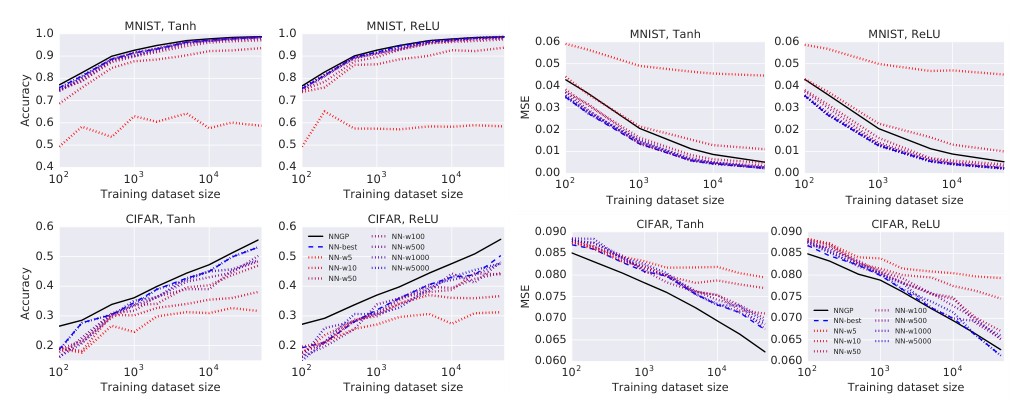
Figure 1: The NNGP often outperforms finite width networks, and neural network performance more closely resembles NNGP performance with increasing width. Test accuracy and mean squared error on MNIST and CIFAR-10 dataset are shown for the best performing NNGP and best performing SGD trained neural networks for given width. ‘NN-best’ denotes the best performing (on the validation set) neural network across all widths and trials. Often this is the neural network with the largest width.
图 1:NNGP 常常优于有限宽网络,而且随着宽度增加,神经网络的表现会更接近 NNGP。图中给出给定宽度下,表现最好的 NNGP 与表现最好的、用 SGD 训练的神经网络,在 MNIST 和 CIFAR-10 数据集上的测试精度和均方误差。‘NN-best’ 表示在所有宽度和所有试验中(按验证集)表现最好的神经网络。这往往就是宽度最大的那个网络。
We additionally find the performance of the best finite-width NNs, trained with a variant of SGD, approaches that of the NNGP with increasing layer width. This is interesting from at least two, potentially related, standpoints. (1) NNs are commonly believed to be powerful because of their ability to do flexible representation learning, while our NNGP uses fixed basis functions; nonetheless, in our experiments we find no salient performance advantage to the former. (2) It hints at a possible relationship between SGD and Bayesian inference in certain regimes – were the neural networks trained in a fully Bayesian fashion, rather than by SGD, the approach to NNGP in the large width limit would be guaranteed. There is recent work suggesting that SGD can implement approximate Bayesian inference (Mandt et al. 2017) under certain assumptions.
我们还发现,用一种 SGD 变体训练的最佳有限宽神经网络,其表现会随着层宽增加而接近 NNGP。这一点至少从两个、并且可能相互关联的角度看都有意思。(1)人们通常认为神经网络之所以有力,是因为它们能灵活地做表征学习,而我们的 NNGP 使用固定基函数;尽管如此,在我们的实验中,前者并没有表现出明显的性能优势。(2)它暗示在某些机制下,SGD 与贝叶斯推断之间可能存在联系——若神经网络是以完全贝叶斯的方式、而不是用 SGD 训练的,则在大宽度极限下趋近 NNGP 是有保证的。已有近期工作表明,在一定假定下,SGD 可以实现近似贝叶斯推断(Mandt et al. (2017))。
The similarity of the performance of the widest NN in Figure 1 with the NNGP suggests that the limit of infinite network width, which is inherent to the GP, is far from being a disadvantage. Indeed, in practice it is found that the best generalizing NNs are in fact the widest. To support this, in Figure 2 we show generalization gap results from an experiment in which we train 180 fully-connected networks with five hidden layers on CIFAR-10 with a range of layer widths. For this experiment, we trained the networks using a standard cross entropy loss rather than MSE, leading to a slight difference in performance.
图 1 中最宽神经网络与 NNGP 表现相近,说明高斯过程所固有的无限宽极限远非劣势。事实上,实践中发现泛化最好的神经网络往往正是最宽的那些。为支持这一点,图 2 给出了一项实验的泛化间隙结果:我们在 CIFAR-10 上训练了 180 个有五个隐层、层宽不等的全连接网络。该实验使用标准交叉熵损失而非 MSE,因此表现上会有轻微差别。
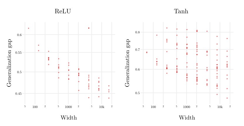
Figure 2: Generalization gap for five hidden layer fully-connected networks with variable widths, using ReLU and Tanh nonlinearities on CIFAR-10. Random optimization and initialization hyperparameters were used and results were filtered for networks with 100% classification training accuracy, resulting in a total of 125 Tanh and 55 ReLU networks. The best generalizing networks are consistently the widest.
图 2:在 CIFAR-10 上,使用 ReLU 和 Tanh 非线性、隐层数为五且宽度可变的全连接网络的泛化间隙。优化和初始化超参数为随机选取,并筛出分类训练精度达到 100% 的网络,最终得到 125 个 Tanh 网络和 55 个 ReLU 网络。泛化最好的网络始终是最宽的那些。
Uncertainty: One benefit in using a GP is that, due to its Bayesian nature, all predictions have uncertainty estimates (Equation 9). For conventional neural networks, capturing the uncertainty in a model’s predictions is challenging (Gal 2016). In the NNGP, every test point has an explicit estimate of prediction variance associated with it (Equation 9). In our experiments, we observe that the NNGP uncertainty estimate is highly correlated with prediction error (Figure 3).
不确定度:使用高斯过程的一个好处是,由于其贝叶斯性质,所有预测都带有不确定度估计(式 9)。对常规神经网络来说,刻画模型预测中的不确定度是困难的(Gal (2016))。在 NNGP 中,每个测试点都有与之相伴的预测方差的显式估计(式 9)。在我们的实验中,我们观察到 NNGP 的不确定度估计与预测误差高度相关(图 3)。
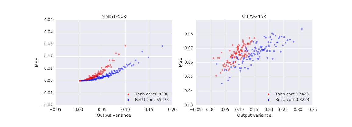
Figure 3: The Bayesian nature of NNGP allows it to assign a prediction uncertainty to each test point. This prediction uncertainty is highly correlated with the empirical error on test points. The -axis shows the predicted MSE for test points, while the -axis shows the realized MSE. To allow comparison of mean squared error, each plotted point is an average over 100 test points, binned by predicted MSE. The hyperparameters for the NNGP are depth , , and . See Appendix Figure 8 for dependence on training set size.
图 3:NNGP 的贝叶斯性质使它能够给每个测试点赋予预测不确定度。这一预测不确定度与测试点上的经验误差高度相关。横轴为测试点的预测均方误差,纵轴为实际实现的均方误差。为便于比较均方误差,图中每个点是按预测均方误差分箱后、对 100 个测试点的平均。该 NNGP 的超参数为深度 ,,。对训练集大小的依赖见附录图 8。
Table 1: The NNGP often outperforms finite width networks. Test accuracy on MNIST and CIFAR-10 datasets. The reported NNGP results correspond to the best performing depth, , and values on the validation set. The traditional NN results correspond to the best performing depth, width and optimization hyperparameters. Best models for a given training set size are specified by (depth-width--) for NNs and (depth–-) for GPs. More results are in Appendix Table 2.
| Num training | Model (ReLU) | Test accuracy | Model (tanh) | Test accuracy |
|---|---|---|---|---|
| MNIST:1k | NN-2-5000-3.19-0.00 | 0.9252 | NN-2-1000-0.60-0.00 | 0.9254 |
| GP-20-1.45-0.28 | 0.9279 | GP-20-1.96-0.62 | 0.9266 | |
| MNIST:10k | NN-2-2000-0.42-0.16 | 0.9771 | NN-2-2000-2.41-1.84 | 0.9745 |
| GP-7-0.61-0.07 | 0.9765 | GP-2-1.62-0.28 | 0.9773 | |
| MNIST:50k | NN-2-2000-0.60-0.44 | 0.9864 | NN-2-5000-0.28-0.34 | 0.9857 |
| GP-1-0.10-0.48 | 0.9875 | GP-1-1.28-0.00 | 0.9879 | |
| CIFAR:1k | NN-5-500-1.29-0.28 | 0.3225 | NN-1-200-1.45-0.12 | 0.3378 |
| GP-7-1.28-0.00 | 0.3608 | GP-50-2.97-0.97 | 0.3702 | |
| CIFAR:10k | NN-5-2000-1.60-1.07 | 0.4545 | NN-1-500-1.48-1.59 | 0.4429 |
| GP-5-2.97-0.28 | 0.4780 | GP-7-3.48-2.00 | 0.4766 | |
| CIFAR:45k | NN-3-5000-0.53-0.01 | 0.5313 | NN-2-2000-1.05-2.08 | 0.5034 |
| GP-3-3.31-1.86 | 0.5566 | GP-3-3.48-1.52 | 0.5558 |
表 1:NNGP 常常优于有限宽网络。表中为 MNIST 和 CIFAR-10 数据集上的测试精度。所报告的 NNGP 结果对应于验证集上表现最好的深度、 和 。传统神经网络结果对应于表现最好的深度、宽度和优化超参数。对给定训练集大小,最佳模型对神经网络记为(深度-宽度--),对高斯过程记为(深度–-)。更多结果见附录表 2。
| Num training | Model (ReLU) | Test accuracy | Model (tanh) | Test accuracy |
|---|---|---|---|---|
| MNIST:1k | NN-2-5000-3.19-0.00 | 0.9252 | NN-2-1000-0.60-0.00 | 0.9254 |
| GP-20-1.45-0.28 | 0.9279 | GP-20-1.96-0.62 | 0.9266 | |
| MNIST:10k | NN-2-2000-0.42-0.16 | 0.9771 | NN-2-2000-2.41-1.84 | 0.9745 |
| GP-7-0.61-0.07 | 0.9765 | GP-2-1.62-0.28 | 0.9773 | |
| MNIST:50k | NN-2-2000-0.60-0.44 | 0.9864 | NN-2-5000-0.28-0.34 | 0.9857 |
| GP-1-0.10-0.48 | 0.9875 | GP-1-1.28-0.00 | 0.9879 | |
| CIFAR:1k | NN-5-500-1.29-0.28 | 0.3225 | NN-1-200-1.45-0.12 | 0.3378 |
| GP-7-1.28-0.00 | 0.3608 | GP-50-2.97-0.97 | 0.3702 | |
| CIFAR:10k | NN-5-2000-1.60-1.07 | 0.4545 | NN-1-500-1.48-1.59 | 0.4429 |
| GP-5-2.97-0.28 | 0.4780 | GP-7-3.48-2.00 | 0.4766 | |
| CIFAR:45k | NN-3-5000-0.53-0.01 | 0.5313 | NN-2-2000-1.05-2.08 | 0.5034 |
| GP-3-3.31-1.86 | 0.5566 | GP-3-3.48-1.52 | 0.5558 |
3.2 Relationship to Deep Signal Propagation
3.2 与深度信号传播的关系
Several prior works (Poole et al. (2016); Schoenholz et al. (2017); Daniely et al. 2016; Duvenaud et al. 2014) have noted the recurrence relations Equation 5 commonly approach a functionally uninteresting fixed point with depth , in that becomes a constant or piecewise constant map. We now briefly relate our ability to train NNGPs with the convergence of to the fixed-point kernel.
若干先前工作(Poole et al. (2016);Schoenholz et al. (2017);Daniely et al. (2016);Duvenaud et al. (2014))已经指出,式 5 的递推关系在深度 时,通常会趋向一个功能上乏味的不动点,也就是说 会变成一个常数或分段常数映射。下面我们把训练 NNGP 的能力,与 向不动点核的收敛简要联系起来。
We will be particularly interested in contextualizing our results in relation to Poole et al. (2016); Schoenholz et al. (2017) which analyzed the fixed points and the approach to them in detail for bounded nonlinearities. To briefly recapitulate: there are regions of hyperparameter space (called phases) where changes only quantitatively with and . However, there are low dimensional boundaries that separate different phases and between them the nature of changes qualitatively.
我们尤其希望把结果放到 Poole et al. (2016);Schoenholz et al. (2017) 的语境中来理解,这两项工作对有界非线性下的不动点及其趋近过程做了细致分析。简要复述如下:在超参数空间的一些区域(称作相)中, 随 和 只发生定量变化。但存在分隔不同相的低维边界,在边界两侧, 的性质会发生定性变化。
For the Tanh nonlinearity, there are two distinct phases respectively called the “ordered” phase and the “chaotic” phase that can be understood as a competition between the weights and the biases of the network. A diagram showing these phases and the boundary between them is shown in Figure 4(a). In the ordered phase, the features obtained by propagating an input through the each layer of the recursion become similar for dissimilar inputs. Fundamentally, this occurs because the different inputs share common bias vectors and so all inputs end up just approaching the random bias. In this case the covariance for every pair of inputs , where is a constant that depends only on and . All inputs have unit correlation asymptotically with depth. By contrast in the chaotic phase the weight variance dominates and similar inputs become dissimilar with depth as they are randomly projected by the weight matrices. In this case, the covariance for but for . Here is the fixed point correlation. In each of these regimes, there is also a finite depth-scale which describes the characteristic number of layers over which the covariance function decays exponentially towards its fixed point form. Exactly at the boundary between these two regimes is a line in -space where the decay towards its fixed point is significantly slower and non-exponential. It was noted in Schoenholz et al. (2017) that this approach to the fixed-point covariance fundamentally bounded whether or not neural networks could successfully be trained. It was shown that initializing networks on this line allowed for significantly deeper neural networks to be trained.
对 Tanh 非线性,存在两个不同的相,分别称为“有序”相和“混沌”相,可以理解为网络权重与偏置之间的竞争。展示这两个相及其分界的图见图 4(a)。在有序相中,把一个输入沿递推的各层向前传播后得到的特征,即使输入原本不同,也会变得相似。从根本上说,这是因为不同输入共享共同的偏置向量,于是所有输入最终都只是趋近这个随机偏置。此时,对每一对输入 ,协方差 ,其中 是一个只依赖于 和 的常数。随着深度增加,所有输入渐近地具有单位相关。相反,在混沌相中,权重方差 占主导,相近的输入会随着深度增加、被权重矩阵随机投影而变得不再相似。此时,当 时协方差 ,而当 时则趋向 。这里 是不动点相关。在这两个区域内,还有一个有限的深度尺度 ,用来描述协方差函数向其不动点形式做指数衰减的特征层数。恰好在这两个区域的边界上,在 空间中有一条线,沿这条线, 向不动点的衰减显著更慢,而且不再是指数的。Schoenholz et al. (2017) 指出,向不动点协方差的这一趋近过程,从根本上限制了神经网络能否被成功训练。他们还表明,把网络初始化在这条线上,可以训练显著更深的神经网络。
For ReLU networks a similar picture emerges, however there are some subtleties due to the unbounded nature of the nonlinearity. In this case for all and , for all and every point becomes asymptotically correlated. Despite this, there are again two phases: a “bounded” phase in which is finite (and nonzero) and an unbounded phase in which is either infinite or zero. As in the Tanh case there are depth scales that control the rate of convergence to these fixed points and therefore limit the maximum trainable depth. The phase diagram for the ReLU nonlinearity is also shown in Figure 4(b).
对 ReLU 网络,也会出现类似的图景,不过由于非线性无界,情况有些微妙。此时,对所有 和 ,都有 对一切 成立,每个点都会渐近相关。尽管如此,仍然存在两个相:一个“有界”相,其中 有限(且非零);以及一个无界相,其中 要么是无穷,要么是零。与 Tanh 情形一样,也存在控制向这些不动点收敛速度、从而限制最大可训练深度的深度尺度。ReLU 非线性的相图同样画在图 4(b) 中。
In a striking analogy with the trainability of neural networks, we observe that the performance of the NNGP appears to closely track the structure from the phase diagram, clearly illustrated in Figure 4. Indeed, we see that as for hyperparameter settings that are far from criticality, the GP is unable to train and we encounter poor test set performance. By contrast, near criticality we observe that our models display high accuracy. Moreover, we find that the accuracy appears to drop more quickly away from the phase boundary with increase in depth of the GP kernel, . To understand this effect we note that information about data will be available to our model only through the difference . However, as the depth gets larger, this difference becomes increasingly small and at some point can no longer be represented due to numerical precision. At this point our test accuracy begins to quickly degrade to random chance.
与神经网络的可训练性形成一种惊人的类比,我们观察到 NNGP 的表现似乎紧密跟随相图中的结构,这在图 4 中可以清楚地看到。事实上,当超参数设置远离临界性时,高斯过程无法训练,测试表现很差。相反,在临界性附近,我们的模型表现出高准确率。此外我们还发现,随着高斯过程核 的深度 增加,准确率在离开相边界时下降得更快。要理解这一效应,只需注意到,关于数据的信息只能通过差值 进入我们的模型。然而,随着深度变大,这一差值会越来越小,到某一点就不再能被数值精度表示。此时,测试准确率开始迅速退化到随机猜测的水平。
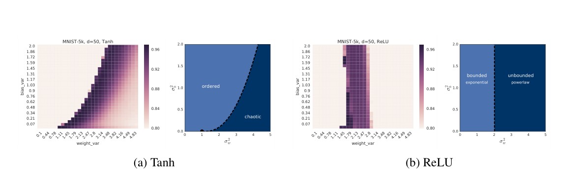
Figure 4: The best performing NNGP hyperparameters agree with those predicted by deep signal propagation. Test set accuracy heatmaps for NNGPs evaluated for a grid of and values. The right plot in each subfigure (a), (b) is a theoretical phase diagram for that nonlinearity following the methodology of Schoenholz et al. (2017). We observe that the performance of the NNGP is best along the critical line (dotted lines). Additional depths are shown in the Appendix Figure 9.
图 4:表现最好的 NNGP 超参数,与深度信号传播所预言的相一致。图中是对一组 和 网格评估得到的 NNGP 测试精度热图。每个子图 (a)、(b) 中右侧的图,是按 Schoenholz et al. (2017) 的方法得到的该非线性的理论相图。我们观察到,NNGP 的表现在临界线(虚线)上最好。更多深度见附录图 9。
4 Conclusion and Future Directions
4 结论与未来方向
By harnessing the limit of infinite width, we have specified a correspondence between priors on deep neural networks and Gaussian processes whose kernel function is constructed in a compositional, but fully deterministic and differentiable, manner. Use of a GP prior on functions enables exact Bayesian inference for regression from matrix computations, and hence we are able to obtain predictions and uncertainty estimates from deep neural networks without stochastic gradient-based training. The performance is competitive with the best neural networks (within specified class of fully-connected models) trained on the same regression task under similar hyperparameter settings. While we were able to run experiments for somewhat large datasets (sizes of 50k), we intend to look into scalability for larger learning tasks, possibly harnessing recent progress in scalable GPs (Quiñonero-Candela & Rasmussen 2005; Hensman et al. 2013).
通过利用无限宽极限,我们给出了深度神经网络先验与一类高斯过程之间的对应,这类高斯过程的核函数以组合的方式构造,但完全是确定且可微的。使用函数上的高斯过程先验,使得回归中的精确贝叶斯推断可以由矩阵计算完成,因而我们可以在不做基于随机梯度的训练的情况下,从深度神经网络得到预测和不确定度估计。在指定的全连接模型类内,其表现可以与在同一回归任务、相近超参数设置下训练的最佳神经网络相竞争。虽然我们已经能在规模约 5 万的较大数据集上做实验,我们仍打算考察更大学习任务上的可扩展性,或可利用近年来可扩展高斯过程的进展(Quiñonero-Candela & Rasmussen (2005);Hensman et al. (2013))。
In our experiments, we observed the performance of the optimized neural network appears to approach that of the GP computation with increasing width. Whether gradient-based stochastic optimization implements an approximate Bayesian computation is an interesting question (Mandt et al. 2017). Further investigation is needed to determine if SGD does approximately implement Bayesian inference under the conditions typically employed in practice.
在实验中我们观察到,经过优化的神经网络,其表现似乎会随着宽度增加而接近高斯过程的计算结果。基于梯度的随机优化是否实现了一种近似贝叶斯计算,是一个有意思的问题(Mandt et al. (2017))。还需要进一步研究,才能确定在实践中通常采用的条件下,SGD 是否近似地实现了贝叶斯推断。
Additionally, the NNGP provides explicit estimates of uncertainty. This may be useful in predicting model failure in critical applications of deep learning, or for active learning tasks where it can be used to identify the best datapoints to hand label.
此外,NNGP 还给出不确定度的显式估计。这在预测深度学习关键应用中的模型失效时可能有用,也可以用于主动学习任务,用来找出最值得人工标注的数据点。
Acknowledgments
致谢
We thank Ryan Adams, Samy Bengio, and Matt Hoffman for useful discussions and feedback, and Gamaleldin Elsayed and Daniel Levy for helpful comments on the manuscript.
我们感谢 Ryan Adams、Samy Bengio 和 Matt Hoffman 提供的有益讨论与反馈,并感谢 Gamaleldin Elsayed 和 Daniel Levy 对稿件提出的意见。
References
参考文献
Maruan Al-Shedivat, Andrew Gordon Wilson, Yunus Saatchi, Zhiting Hu, and Eric P Xing. Learning scalable deep kernels with recurrent structure. Journal of Machine Learning Research, 18(82):1–37, 2017.
Thang Bui, Daniel Hernández-Lobato, Jose Hernandez-Lobato, Yingzhen Li, and Richard Turner. Deep gaussian processes for regression using approximate expectation propagation. In International Conference on Machine Learning, pp. 1472–1481, 2016.
Youngmin Cho and Lawrence K Saul. Kernel methods for deep learning. In Advances in neural information processing systems, pp. 342–350, 2009.
Andreas Damianou and Neil Lawrence. Deep gaussian processes. In Artificial Intelligence and Statistics, pp. 207–215, 2013.
Amit Daniely, Roy Frostig, and Yoram Singer. Toward deeper understanding of neural networks: The power of initialization and a dual view on expressivity. In Advances In Neural Information Processing Systems, pp. 2253–2261, 2016.
de G. Matthews et al. (2018) Alexander G. de G. Matthews, Jiri Hron, Mark Rowland, Richard E. Turner, and Zoubin Ghahramani. Gaussian process behaviour in wide deep neural networks. In International Conference on Learning Representations, 2018. URL https://openreview.net/forum?id=H1-nGgWC-.
David Duvenaud, Oren Rippel, Ryan Adams, and Zoubin Ghahramani. Avoiding pathologies in very deep networks. In Artificial Intelligence and Statistics, pp. 202–210, 2014.
Yarin Gal. Uncertainty in deep learning. PhD thesis, PhD thesis, University of Cambridge, 2016.
Yarin Gal and Zoubin Ghahramani. Dropout as a bayesian approximation: Representing model uncertainty in deep learning. In international conference on machine learning, pp. 1050–1059, 2016.
Daniel Golovin, Benjamin Solnik, Subhodeep Moitra, Greg Kochanski, John Karro, and D Sculley. Google vizier: A service for black-box optimization. In Proceedings of the 23rd ACM SIGKDD International Conference on Knowledge Discovery and Data Mining, pp. 1487–1495. ACM, 2017.
Tamir Hazan and Tommi Jaakkola. Steps toward deep kernel methods from infinite neural networks. arXiv preprint arXiv:1508.05133, 2015.
James Hensman and Neil D Lawrence. Nested variational compression in deep gaussian processes. arXiv preprint arXiv:1412.1370, 2014.
James Hensman, Nicolo Fusi, and Neil D Lawrence. Gaussian processes for big data. arXiv preprint arXiv:1309.6835, 2013.
Diederik Kingma and Jimmy Ba. Adam: A method for stochastic optimization. arXiv preprint arXiv:1412.6980, 2014.
Karl Krauth, Edwin V Bonilla, Kurt Cutajar, and Maurizio Filippone. Autogp: Exploring the capabilities and limitations of gaussian process models. arXiv preprint arXiv:1610.05392, 2016.
Neil D Lawrence and Andrew J Moore. Hierarchical gaussian process latent variable models. In Proceedings of the 24th international conference on Machine learning, pp. 481–488. ACM, 2007.
Stephan Mandt, Matthew D Hoffman, and David M Blei. Stochastic gradient descent as approximate bayesian inference. arXiv preprint arXiv:1704.04289, 2017.
Radford M. Neal. Priors for infinite networks (tech. rep. no. crg-tr-94-1). University of Toronto, 1994a.
Radford M. Neal. Bayesian Learning for Neural Networks. PhD thesis, University of Toronto, Dept. of Computer Science, 1994b.
Ben Poole, Subhaneil Lahiri, Maithra Raghu, Jascha Sohl-Dickstein, and Surya Ganguli. Exponential expressivity in deep neural networks through transient chaos. In Advances In Neural Information Processing Systems, pp. 3360–3368, 2016.
Joaquin Quiñonero-Candela and Carl Edward Rasmussen. A unifying view of sparse approximate gaussian process regression. Journal of Machine Learning Research, 6(Dec):1939–1959, 2005.
Carl Edward Rasmussen and Christopher KI Williams. Gaussian processes for machine learning, volume 1. MIT press Cambridge, 2006.
Ryan Rifkin and Aldebaro Klautau. In defense of one-vs-all classification. Journal of machine learning research, 5(Jan):101–141, 2004.
Ryan Rifkin, Gene Yeo, Tomaso Poggio, et al. Regularized least-squares classification. Nato Science Series Sub Series III Computer and Systems Sciences, 190:131–154, 2003.
Samuel S Schoenholz, Justin Gilmer, Surya Ganguli, and Jascha Sohl-Dickstein. Deep information propagation. ICLR, 2017.
Christopher KI Williams. Computing with infinite networks. In Advances in neural information processing systems, pp. 295–301, 1997.
Christopher KI Williams and David Barber. Bayesian classification with gaussian processes. IEEE Transactions on Pattern Analysis and Machine Intelligence, 20(12):1342–1351, 1998.
Andrew G Wilson, Zhiting Hu, Ruslan R Salakhutdinov, and Eric P Xing. Stochastic variational deep kernel learning. In Advances in Neural Information Processing Systems, pp. 2586–2594, 2016a.
Andrew Gordon Wilson, Zhiting Hu, Ruslan Salakhutdinov, and Eric P Xing. Deep kernel learning. In Artificial Intelligence and Statistics, pp. 370–378, 2016b.
Appendix A Draws from an NNGP prior
附录 A 从 NNGP 先验中抽样
Figure 5 illustrates the nature of the GP prior for the ReLU nonlinearity by depicting samples of 1D functions drawn from a ReLU GP, , with fixed depth and .
图 5 通过画出从 ReLU 高斯过程 中抽出的一维函数 样本,来说明 ReLU 非线性下该高斯过程先验的性质;深度固定为 ,且 。
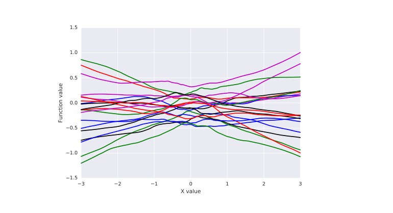
Figure 5: Samples from an NNGP prior for 1D functions. Different lines correspond to different draws (arbitrary colors).
图 5:来自 NNGP 先验的一维函数样本。不同曲线对应不同的抽取(颜色任意)。
Appendix B Analytic Form for Kernel and Comparison
附录 B 核的解析形式及比较
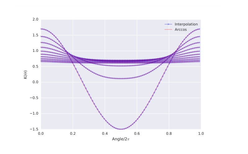
Figure 6: The angular structure of the kernel and its evolution with depth. Also illustrated is the good agreement between the kernel computed using the methods of Section 2.5 (blue, starred) and the analytic form of the kernel (red). The depth in runs from (flattened curves for increasing ), and .
图 6:核的角度结构及其随深度的演变。图中也展示了用第 2.5 节方法算出的核(蓝色,带星号)与核的解析形式(红色)之间的良好吻合。 中的深度 取 (曲线随 增加而变平),且 。
In the main text, we noted that the recurrence relation Equation 5 can be computed analytically for certain nonlinearities. In particular, this was computed in Cho & Saul (2009) for polynomial rectified nonlinearities. For ReLU, the result including the weight and bias variance is
在正文中我们指出,对某些非线性,式 5 的递推关系可以解析计算。特别地,Cho & Saul (2009) 为多项式整流非线性计算了这一结果。对 ReLU,把权重和偏置方差包括在内的结果是
To illustrate the angular form of and its evolution with , in Figure 6 we plot for the ReLU nonlinearity, where is the angle between and with norms such that . We observe a flattening of the angular structure with increase in depth , as predicted from the understanding in Section 3.2. Simultaneously, the figure also illustrates the good agreement between the kernel computed using the numerical implementation of Section 2.5 (blue, starred) and the analytic arccosine kernel, Equation 11 (red), for a particular choice of hyperparameters .
为说明 的角度形式及其随 的演变,我们在图 6 中画出 ReLU 非线性下的 ,其中 是 与 之间的夹角,且范数满足 。我们观察到,随着深度 增加,角度结构会变平,这与第 3.2 节中的理解相符。与此同时,该图还展示了用第 2.5 节的数值实现算出的核(蓝色,带星号)与解析的反余弦核(式 11,红色)之间的良好吻合,超参数取某一组 。
Appendix C Bayesian marginalization over intermediate layers
附录 C 对中间层做贝叶斯边缘化
In this section, we present an alternate derivation of the equivalence between infinitely wide deep neural networks and Gaussian process by marginalization over intermediate layers. For this derivation, we take the weight and bias parameters to be drawn from independent Gaussians, with zero mean and appropriately scaled variance.
本节给出无限宽深度神经网络与高斯过程等价性的另一种推导,即对中间层做边缘化。在这一推导中,我们把权重和偏置参数取为从独立高斯中抽出,均值为零,方差做适当缩放。
We are interested in finding the distribution over network outputs , conditioned on network inputs , for input dimensionality , output dimensionality , and dataset size . Intervening layers will have width , for . We define the second moment matrix (here post-nonlinearity) for each layer to be
我们关心的是,在给定网络输入 时,网络输出 的分布 ,其中 为输入维, 为输出维, 为数据集大小。中间层宽度为 ,对 有 。我们把每一层 的二阶矩矩阵(此处是非线性之后的)定义为
$$K^{l}{ab} =\left{\begin{array}[]{ccc}\frac{1}{d{\text{in}}}\sum_{n}x_{na}x_{nb}&&l=0\
\frac{1}{N_{l}}\sum_{n}\phi(z_{na}^{l-1})\phi(z_{nb}^{l-1})&&l>0\end{array}\right..$$
Our approach is to think of intermediate random variables corresponding to these second moments defined above. By definition, only depends on . In turn, the pre-activations are described by a Gaussian process conditioned on the second moment matrix ,
我们的做法是,把与上面定义的这些二阶矩相对应的量,看作中间随机变量。按定义, 只依赖于 。反过来,预激活 在给定二阶矩矩阵 时,由一个高斯过程描述,
where
其中
This correspondence of each layer to a GP, conditioned on the layer’s second moment matrix, is exact even for finite width because the parameters are drawn from a Gaussian. Altogether, this justifies the graphical model depicted in Figure 7.
每一层在给定该层二阶矩矩阵时对应于一个高斯过程,这一对应即使在有限宽度 下也是精确的,因为参数是从高斯中抽出的。合在一起,这就给出了图 7 所示的图模型。
We will write as an integral over all the intervening second moment matrices ,
我们将把 写成对所有中间二阶矩矩阵 的积分,
This joint distribution can be decomposed as
这一联合分布可以分解为
The directed decomposition in Equation 17 holds because is a function only of (see Equation C), depends only on (see Equation 14), is a function only of , etc (Figure 7).
式 17 中的有向分解之所以成立,是因为 只是 的函数(见式 C), 只依赖于 (见式 14), 又只是 的函数,以此类推(图 7)。
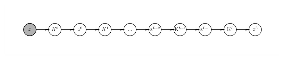
Figure 7: Graphical model for neural network’s computation.
图 7:神经网络计算的图模型。
The sum in Equation C for is a sum over i.i.d. terms. As grows large, the Central Limit Theorem applies, and converges to a Gaussian with variance that shrinks as . Further, in the infinite width limit it will go to a delta function,
式 C 中当 时的求和,是对独立同分布项求和。当 变大时,中心极限定理适用, 收敛到一个方差按 缩小的高斯。进一步,在无限宽极限下,它会变成一个 delta 函数,
with defined as in Equation 5. Similarly, the dependence of on can be expressed as a delta function,
其中 的定义与式 5 相同。类似地, 对 的依赖也可以写成一个 delta 函数,
Substituting , and into Equation 17, we get
把 、 和 代入式 17,得到
So, in the limit of infinite width, is described by a Gaussian process with kernel .
因此,在无限宽极限下, 由一个核为 的高斯过程描述。
Appendix D Details of the Experiments
附录 D 实验细节
We outline details of the experiments for Section 3. For MNIST we use a 50k/10k/10k split of the training/validation/test dataset. For CIFAR-10, we used a 45k/5k/10k split. The validation set was used for choosing the best hyperparameters and evaluation on the test set is reported.
我们概述第 3 节实验的细节。对 MNIST,我们使用 50k/10k/10k 的训练/验证/测试划分。对 CIFAR-10,我们使用 45k/5k/10k 的划分。验证集用来选择最佳超参数,并报告在测试集上的评估。
For training neural networks hyperparameters were optimized via random search on average 250 trials for each choice of (, depth, width, nonlinearity).
训练神经网络时,超参数通过随机搜索优化,对每一组 平均做 250 次试验。
Random search range: Learning rate was sampled within in log-scale, weight decay constant was sampled from in log-scale, , was uniformly sampled and mini-batch size was chosen equally among .
随机搜索范围:学习率在对数尺度上从 中采样,权重衰减常数在对数尺度上从 中采样,, 做均匀采样,小批量大小在 中等概率选取。
For the GP with given depth and nonlinearity, a grid of 30 points evenly spaced from 0.1 to 5.0 (for ) and 30 points evenly spaced from 0 to 2.0 (for ) was evaluated to generate the heatmap. The best GP run was chosen among the 900 evaluations in the - grid.
对给定深度和非线性的高斯过程,为生成热图,我们在 上从 0.1 到 5.0 均匀取 30 个点,在 上从 0 到 2.0 均匀取 30 个点并做评估。最佳高斯过程运行是在 – 网格的 900 次评估中选出的。
Computation time: We report computation times for NNGP experiments. The grid generation with took 440-460s with 6 CPUs for , which was amortized over all the experiments. For full (50k) MNIST, constructing for each layer took 90-140s (depending on CPU generation) running on 64 CPUs. Solving linear equations via Cholesky decomposition took 180-220s for 1000 test points.
计算时间:我们报告 NNGP 实验的计算时间。网格生成在 6 个 CPU 上、当 时用了 440–460 秒,这一代价由全部实验摊还。对完整(5 万)MNIST,在 64 个 CPU 上为每一层构造 用了 90–140 秒(取决于 CPU 代数)。用 Cholesky 分解求解线性方程、针对 1000 个测试点,用了 180–220 秒。
Details of NNGP implementaion: For all the experiments we used pre-computed lookup tables with and . Default value for the target noise was set to and was increased by factor of 10 when Cholesky decomposition failed while solving Equation 8 and 9. We refer to Rasmussen & Williams (2006) for standard numerically stable implementation of GP regression.
NNGP 实现细节:所有实验都使用预先计算的查找表 ,参数为 ,以及 。目标噪声 的默认值设为 ,在求解式 8 和式 9 时若 Cholesky 分解失败,则把它乘以 10。关于高斯过程回归的标准数值稳定实现,我们参考 Rasmussen & Williams (2006)。
Appendix E Further results
附录 E 更多结果
Here we include more results from experiments described in Section 3.
这里补充第 3 节所述实验的更多结果。
Uncertainty: Relationship between the target MSE and the GP’s uncertainty estimate for smaller training set size is shown in Figure 8.
不确定度:更小训练集下,目标均方误差与高斯过程不确定度估计之间的关系见图 8。
Performance: Performance of grid points of - for varying depth is shown in Figure 9. The best performing NNGP’s hyperparameters are distributed near the critical line (Figure 10) where the phase changes as described in Section 3.2.
表现:– 网格点在不同深度下的表现见图 9。表现最好的 NNGP 的超参数分布在临界线附近(图 10),相变情况如第 3.2 节所述。
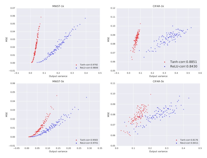
Figure 8: The prediction uncertainty for smaller number of training points. The details are the same as Figure 3.
图 8:训练点数更少时的预测不确定度。细节与图 3 相同。
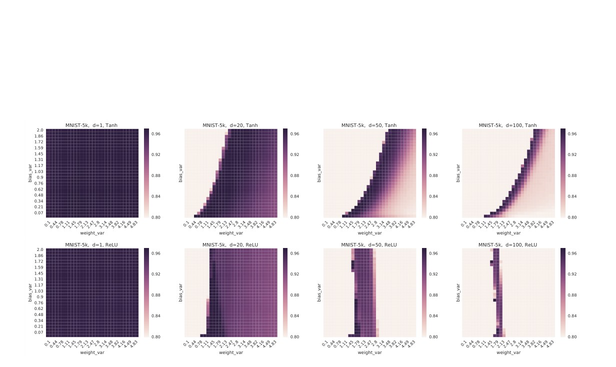
Figure 9: Test set accuracy heatmaps for NNGPs evaluated for a grid of and values for varying depth. Rows correspond to Tanh and ReLU nonlinearities, and columns correspond to varying depth.
图 9:在不同深度下,对一组 和 网格评估得到的 NNGP 测试精度热图。行对应 Tanh 和 ReLU 非线性,列对应不同深度。
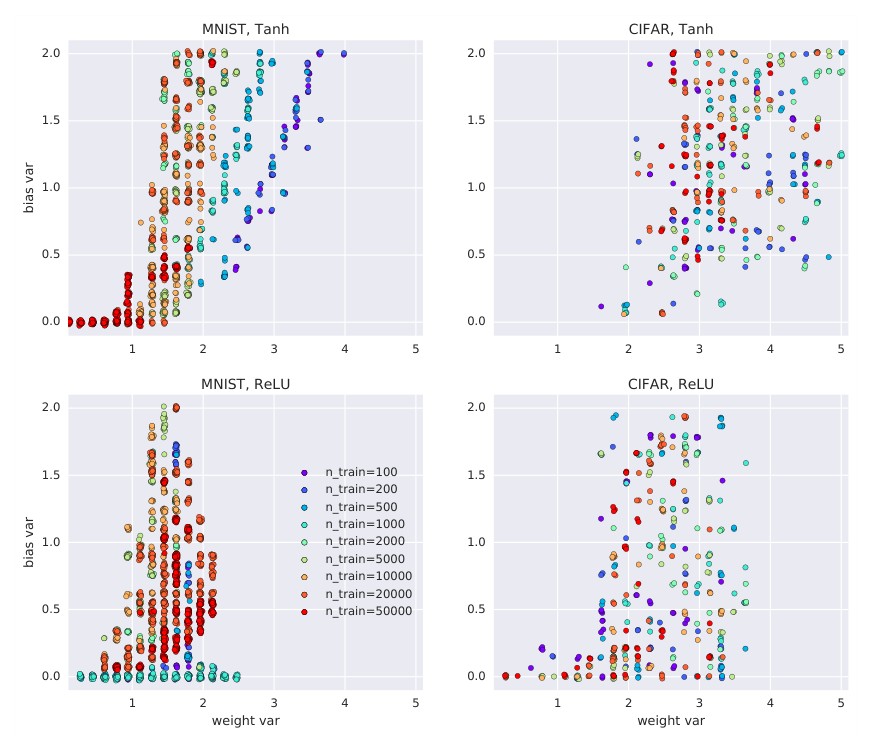
Figure 10: Best performing NNGPs are distributed near the critical line. Weight and bias variance distribution for the 25 best performing runs for NNGP with the given training set size is shown.
图 10:表现最好的 NNGP 分布在临界线附近。图中给出给定训练集大小下,NNGP 表现最好的 25 次运行的权重方差和偏置方差分布。
Table 2: Completion of Table 1. The reported NNGP results correspond to the best performing depth, , and values on the validation set. The traditional NN results correspond to the best performing depth, width and optimization hyperparameters. Best models for a given training set size are specified by (depth-width--) for NNs and (depth–-) for GPs.
| Num training | Model (ReLU) | Test accuracy | Model (tanh) | Test accuracy |
|---|---|---|---|---|
| MNIST:100 | NN-2-5000-0.10-0.11 | 0.7786 | NN-1-500-1.48-0.61 | 0.7766 |
| GP-100-1.79-0.83 | 0.7735 | GP-100-3.14-0.97 | 0.7736 | |
| MNIST:200 | NN-2-2000-0.52-0.00 | 0.8298 | NN-2-1000-1.80-1.99 | 0.8223 |
| GP-100-1.79-0.83 | 0.8282 | GP-100-3.99-2.00 | 0.8277 | |
| MNIST:500 | NN-2-5000-1.82-0.77 | 0.9028 | NN-1-5000-3.74-2.18 | 0.9001 |
| GP-100-1.79-0.83 | 0.8995 | GP-50-3.48-1.86 | 0.9008 | |
| MNIST:1k | NN-2-5000-3.19-0.00 | 0.9252 | NN-2-1000-0.60-0.00 | 0.9254 |
| GP-20-1.45-0.28 | 0.9279 | GP-20-1.96-0.62 | 0.9266 | |
| MNIST:2k | NN-2-5000-2.88-0.01 | 0.9468 | NN-1-2000-0.98-1.30 | 0.9462 |
| GP-10-1.11-0.55 | 0.9485 | GP-10-1.79-1.45 | 0.9477 | |
| MNIST:5k | NN-3-500-2.92-0.22 | 0.9675 | NN-2-1000-4.12-2.18 | 0.9655 |
| GP-7-0.61-0.07 | 0.9692 | GP-3-1.11-0.00 | 0.9693 | |
| MNIST:10k | NN-2-2000-0.42-0.16 | 0.9771 | NN-2-2000-2.41-1.84 | 0.9745 |
| GP-7-0.61-0.07 | 0.9765 | GP-2-1.62-0.28 | 0.9773 | |
| MNIST:20k | NN-3-1000-2.45-0.98 | 0.9825 | NN-2-2000-0.21-0.10 | 0.9814 |
| GP-5-1.62-0.83 | 0.9830 | GP-1-2.63-0.00 | 0.9836 | |
| MNIST:50k | NN-2-2000-0.60-0.44 | 0.9864 | NN-2-5000-0.28-0.34 | 0.9857 |
| GP-1-0.10-0.48 | 0.9875 | GP-1-1.28-0.00 | 0.9879 | |
| CIFAR:100 | NN-5-500-1.88-1.00 | 0.2586 | NN-2-200-3.22-2.09 | 0.2470 |
| GP-3-4.49-0.97 | 0.2673 | GP-10-3.65-1.17 | 0.2718 | |
| CIFAR:200 | NN-3-200-0.17-0.00 | 0.2719 | NN-3-200-1.41-0.21 | 0.2686 |
| GP-3-3.99-1.72 | 0.3022 | GP-7-3.65-0.55 | 0.2927 | |
| CIFAR:500 | NN-1-100-1.26-0.63 | 0.3132 | NN-1-2000-0.11-0.90 | 0.2939 |
| GP-20-1.79-0.21 | 0.3395 | GP-7-3.65-0.62 | 0.3291 | |
| CIFAR:1k | NN-5-500-1.29-0.28 | 0.3225 | NN-1-200-1.45-0.12 | 0.3378 |
| GP-7-1.28-0.00 | 0.3608 | GP-50-2.97-0.97 | 0.3702 | |
| CIFAR:2k | NN-3-5000-5.59-0.57 | 0.3894 | NN-5-1000-0.86-1.28 | 0.3597 |
| GP-3-4.16-1.17 | 0.3953 | GP-5-4.66-1.03 | 0.3959 | |
| CIFAR:5k | NN-5-2000-5.26-1.74 | 0.4241 | NN-1-5000-0.07-0.22 | 0.3993 |
| GP-3-4.66-1.03 | 0.4454 | GP-10-3.65-1.38 | 0.4430 | |
| CIFAR:10k | NN-5-2000-1.60-1.07 | 0.4545 | NN-1-500-1.48-1.59 | 0.4429 |
| GP-5-2.97-0.28 | 0.4780 | GP-7-3.48-2.00 | 0.4766 | |
| CIFAR:20k | NN-3-5000-4.18-0.18 | 0.5041 | NN-2-5000-0.02-1.12 | 0.4565 |
| GP-3-5.00-0.83 | 0.5118 | GP-7-3.14-1.93 | 0.5124 | |
| CIFAR:45k | NN-3-5000-0.53-0.01 | 0.5313 | NN-2-2000-1.05-2.08 | 0.5034 |
| GP-3-3.31-1.86 | 0.5566 | GP-3-3.48-1.52 | 0.5558 |
表 2:表 1 的补全。所报告的 NNGP 结果对应于验证集上表现最好的深度、 和 。传统神经网络结果对应于表现最好的深度、宽度和优化超参数。对给定训练集大小,最佳模型对神经网络记为(深度-宽度--),对高斯过程记为(深度–-)。
| Num training | Model (ReLU) | Test accuracy | Model (tanh) | Test accuracy |
|---|---|---|---|---|
| MNIST:100 | NN-2-5000-0.10-0.11 | 0.7786 | NN-1-500-1.48-0.61 | 0.7766 |
| GP-100-1.79-0.83 | 0.7735 | GP-100-3.14-0.97 | 0.7736 | |
| MNIST:200 | NN-2-2000-0.52-0.00 | 0.8298 | NN-2-1000-1.80-1.99 | 0.8223 |
| GP-100-1.79-0.83 | 0.8282 | GP-100-3.99-2.00 | 0.8277 | |
| MNIST:500 | NN-2-5000-1.82-0.77 | 0.9028 | NN-1-5000-3.74-2.18 | 0.9001 |
| GP-100-1.79-0.83 | 0.8995 | GP-50-3.48-1.86 | 0.9008 | |
| MNIST:1k | NN-2-5000-3.19-0.00 | 0.9252 | NN-2-1000-0.60-0.00 | 0.9254 |
| GP-20-1.45-0.28 | 0.9279 | GP-20-1.96-0.62 | 0.9266 | |
| MNIST:2k | NN-2-5000-2.88-0.01 | 0.9468 | NN-1-2000-0.98-1.30 | 0.9462 |
| GP-10-1.11-0.55 | 0.9485 | GP-10-1.79-1.45 | 0.9477 | |
| MNIST:5k | NN-3-500-2.92-0.22 | 0.9675 | NN-2-1000-4.12-2.18 | 0.9655 |
| GP-7-0.61-0.07 | 0.9692 | GP-3-1.11-0.00 | 0.9693 | |
| MNIST:10k | NN-2-2000-0.42-0.16 | 0.9771 | NN-2-2000-2.41-1.84 | 0.9745 |
| GP-7-0.61-0.07 | 0.9765 | GP-2-1.62-0.28 | 0.9773 | |
| MNIST:20k | NN-3-1000-2.45-0.98 | 0.9825 | NN-2-2000-0.21-0.10 | 0.9814 |
| GP-5-1.62-0.83 | 0.9830 | GP-1-2.63-0.00 | 0.9836 | |
| MNIST:50k | NN-2-2000-0.60-0.44 | 0.9864 | NN-2-5000-0.28-0.34 | 0.9857 |
| GP-1-0.10-0.48 | 0.9875 | GP-1-1.28-0.00 | 0.9879 | |
| CIFAR:100 | NN-5-500-1.88-1.00 | 0.2586 | NN-2-200-3.22-2.09 | 0.2470 |
| GP-3-4.49-0.97 | 0.2673 | GP-10-3.65-1.17 | 0.2718 | |
| CIFAR:200 | NN-3-200-0.17-0.00 | 0.2719 | NN-3-200-1.41-0.21 | 0.2686 |
| GP-3-3.99-1.72 | 0.3022 | GP-7-3.65-0.55 | 0.2927 | |
| CIFAR:500 | NN-1-100-1.26-0.63 | 0.3132 | NN-1-2000-0.11-0.90 | 0.2939 |
| GP-20-1.79-0.21 | 0.3395 | GP-7-3.65-0.62 | 0.3291 | |
| CIFAR:1k | NN-5-500-1.29-0.28 | 0.3225 | NN-1-200-1.45-0.12 | 0.3378 |
| GP-7-1.28-0.00 | 0.3608 | GP-50-2.97-0.97 | 0.3702 | |
| CIFAR:2k | NN-3-5000-5.59-0.57 | 0.3894 | NN-5-1000-0.86-1.28 | 0.3597 |
| GP-3-4.16-1.17 | 0.3953 | GP-5-4.66-1.03 | 0.3959 | |
| CIFAR:5k | NN-5-2000-5.26-1.74 | 0.4241 | NN-1-5000-0.07-0.22 | 0.3993 |
| GP-3-4.66-1.03 | 0.4454 | GP-10-3.65-1.38 | 0.4430 | |
| CIFAR:10k | NN-5-2000-1.60-1.07 | 0.4545 | NN-1-500-1.48-1.59 | 0.4429 |
| GP-5-2.97-0.28 | 0.4780 | GP-7-3.48-2.00 | 0.4766 | |
| CIFAR:20k | NN-3-5000-4.18-0.18 | 0.5041 | NN-2-5000-0.02-1.12 | 0.4565 |
| GP-3-5.00-0.83 | 0.5118 | GP-7-3.14-1.93 | 0.5124 | |
| CIFAR:45k | NN-3-5000-0.53-0.01 | 0.5313 | NN-2-2000-1.05-2.08 | 0.5034 |
| GP-3-3.31-1.86 | 0.5566 | GP-3-3.48-1.52 | 0.5558 |