Emerging Properties in Self-Supervised Vision Transformers
Emerging Properties in Self-Supervised Vision Transformers
自监督视觉 Transformer 中涌现的性质
Mathilde Caron Hugo Touvron Ishan Misra Hervé Jegou Affiliation: Facebook AI Research Inria Sorbonne University Julien Mairal Piotr Bojanowski Armand Joulin
Abstract
摘要
In this paper, we question if self-supervised learning provides new properties to Vision Transformer (ViT) [19] that stand out compared to convolutional networks (convnets). Beyond the fact that adapting self-supervised methods to this architecture works particularly well, we make the following observations: first, self-supervised ViT features contain explicit information about the semantic segmentation of an image, which does not emerge as clearly with supervised ViTs, nor with convnets. Second, these features are also excellent -NN classifiers, reaching 78.3% top-1 on ImageNet with a small ViT. Our study also underlines the importance of momentum encoder [33], multi-crop training [10], and the use of small patches with ViTs. We implement our findings into a simple self-supervised method, called DINO, which we interpret as a form of self-distillation with no labels. We show the synergy between DINO and ViTs by achieving 80.1% top-1 on ImageNet in linear evaluation with ViT-Base.
本文追问:自监督学习是否会给 Vision Transformer(ViT)[19] 带来区别于卷积网络(convnets)的新性质。除了把自监督方法迁移到该架构效果特别好之外,我们还有以下观察:其一,自监督 ViT 特征显式包含图像语义分割信息,这在有监督 ViT 或卷积网络上并不同样清晰;其二,这些特征也是出色的 -NN 分类器,用小型 ViT 即可在 ImageNet 上达到 78.3% top-1。研究还强调了动量编码器[33]、multi-crop 训练[10]以及在 ViT 上使用小 patch 的重要性。我们把上述发现落实为一个简单的自监督方法 DINO,可理解为一种无标签自蒸馏(self-distillation with no labels)。凭借 DINO 与 ViT 的协同,ViT-Base 在 ImageNet 线性评估上达到 80.1% top-1。
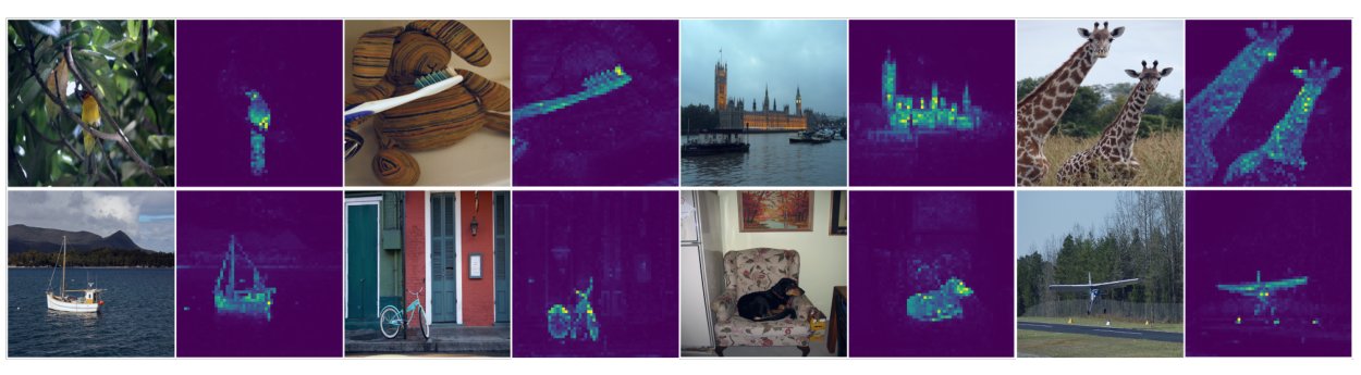
Figure 1: Self-attention from a Vision Transformer with patches trained with no supervision. We look at the self-attention of the [CLS] token on the heads of the last layer. This token is not attached to any label nor supervision. These maps show that the model automatically learns class-specific features leading to unsupervised object segmentations.
图 1:用无监督训练的、 patch 的 Vision Transformer 自注意力。我们查看最后一层各头上 [CLS] token 的自注意力。该 token 未附着任何标签或监督。这些图表明模型会自动学到类别相关特征,并得到无监督目标分割。
1 Introduction
1 引言
Transformers [70] have recently emerged as an alternative to convolutional neural networks (convnets) for visual recognition [19, 69, 83]. Their adoption has been coupled with a training strategy inspired by natural language processing (NLP), that is, pretraining on large quantities of data and finetuning on the target dataset [18, 55]. The resulting Vision Transformers (ViT) [19] are competitive with convnets but, they have not yet delivered clear benefits over them: they are computationally more demanding, require more training data, and their features do not exhibit unique properties.
Transformer[70] 近来成为视觉识别中卷积网络的替代方案[19, 69, 83]。其采用常伴随一套源自自然语言处理(NLP)的训练策略,即在大规模数据上预训练再在目标数据集上微调[18, 55]。由此得到的 Vision Transformer(ViT)[19] 与卷积网络竞争力相当,但尚未展现出清晰优势:计算更重、需要更多训练数据,特征也未表现出独特性质。
In this paper, we question whether the muted success of Transformers in vision can be explained by the use of supervision in their pretraining. Our motivation is that one of the main ingredients for the success of Transformers in NLP was the use of self-supervised pretraining, in the form of close procedure in BERT [18] or language modeling in GPT [55]. These self-supervised pretraining objectives use the words in a sentence to create pretext tasks that provide a richer learning signal than the supervised objective of predicting a single label per sentence. Similarly, in images, image-level supervision often reduces the rich visual information contained in an image to a single concept selected from a predefined set of a few thousand categories of objects [60].
本文追问:Transformer 在视觉上表现平淡,是否可归因于预训练阶段使用了监督。动机在于,NLP 中 Transformer 成功的关键要素之一是自监督预训练,例如 BERT 中的完形填空[18]或 GPT 中的语言建模[55]。这些自监督目标用句子中的词构造代理任务,提供比“每句预测一个标签”更丰富的学习信号。类似地,在图像上,图像级监督往往把丰富视觉信息压成预定义的几千类物体中的单一概念[60]。
While the self-supervised pretext tasks used in NLP are text specific, many existing self-supervised methods have shown their potential on images with convnets [10, 12, 30, 33]. They typically share a similar structure but with different components designed to avoid trivial solutions (collapse) or to improve performance [16]. In this work, inspired from these methods, we study the impact of self-supervised pretraining on ViT features. Of particular interest, we have identified several interesting properties that do not emerge with supervised ViTs, nor with convnets:
NLP 中的自监督代理任务是文本特有的,但许多现有自监督方法已在卷积网络上展示了潜力[10, 12, 30, 33]。它们结构相近,但用不同组件避免平凡解(崩塌)或提升性能[16]。受此启发,我们研究自监督预训练对 ViT 特征的影响。尤为值得注意的是,我们识别出若干在有监督 ViT 或卷积网络上不会涌现的性质:
- • Self-supervised ViT features explicitly contain the scene layout and, in particular, object boundaries, as shown in Figure 1. This information is directly accessible in the self-attention modules of the last block.
- • 自监督 ViT 特征显式包含场景布局,尤其是物体边界,如图 1 所示。该信息可直接从最后一块的自注意力模块中读取。
- • Self-supervised ViT features perform particularly well with a basic nearest neighbors classifier (-NN) without any finetuning, linear classifier nor data augmentation, achieving 78.3% top-1 accuracy on ImageNet.
- • 自监督 ViT 特征在基础最近邻分类器(-NN)上表现特别好——无需任何微调、线性分类器或数据增强,在 ImageNet 上达到 78.3% top-1 准确率。
The emergence of segmentation masks seems to be a property shared across self-supervised methods. However, the good performance with -NN only emerge when combining certain components such as momentum encoder [33] and multi-crop augmentation [10]. Another finding from our study is the importance of using smaller patches with ViTs to improve the quality of the resulting features.
分割掩码的涌现似乎是多种自监督方法的共性。然而,良好的 -NN 性能只在组合动量编码器[33]与 multi-crop 增强[10]等组件时才出现。另一发现是:在 ViT 上使用更小的 patch 对提升特征质量很重要。
Overall, our findings about the importance of these components lead us to design a simple self-supervised approach that can be interpreted as a form of knowledge distillation [35] with no labels. The resulting framework, DINO, simplifies self-supervised training by directly predicting the output of a teacher network—built with a momentum encoder—by using a standard cross-entropy loss. Interestingly, our method can work with only a centering and sharpening of the teacher output to avoid collapse, while other popular components such as predictor [30], advanced normalization [10] or contrastive loss [33] add little benefits in terms of stability or performance. Of particular importance, our framework is flexible and works on both convnets and ViTs without the need to modify the architecture, nor adapt internal normalizations [58].
综合这些组件的重要性,我们设计了一种简单的自监督方法,可理解为无标签的知识蒸馏[35]。得到的框架 DINO 通过标准交叉熵损失直接预测教师网络(由动量编码器构建)的输出,从而简化自监督训练。有趣的是,仅对教师输出做中心化与锐化即可避免崩塌;预测器[30]、复杂归一化[10]或对比损失[33]等流行组件在稳定性或性能上增益有限。尤为重要的是,该框架灵活,可同时用于卷积网络与 ViT,无需改架构,也不必适配内部归一化[58]。
We further validate the synergy between DINO and ViT by outperforming previous self-supervised features on the ImageNet linear classification benchmark with 80.1% top-1 accuracy with a ViT-Base with small patches. We also confirm that DINO works with convnets by matching the state of the art with a ResNet-50 architecture. Finally, we discuss different scenarios to use DINO with ViTs in case of limited computation and memory capacity. In particular, training DINO with ViT takes just two 8-GPU servers over 3 days to achieve on ImageNet linear benchmark, which outperforms self-supervised systems based on convnets of comparable sizes with significantly reduced compute requirements [10, 30].
我们进一步用 ImageNet 线性分类基准验证 DINO 与 ViT 的协同:小 patch 的 ViT-Base 达到 80.1% top-1,超过此前自监督特征。同时确认 DINO 在 ResNet-50 上也能对齐当时最优。最后讨论计算与显存受限时如何用 DINO 训练 ViT。特别地,用两台 8-GPU 服务器训练约 3 天即可在 ImageNet 线性基准达到 ,优于同规模卷积自监督系统,且算力显著更低[10, 30]。
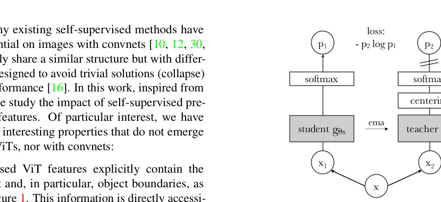
Figure 2: Self-distillation with no labels. We illustrate DINO in the case of one single pair of views (, ) for simplicity. The model passes two different random transformations of an input image to the student and teacher networks. Both networks have the same architecture but different parameters. The output of the teacher network is centered with a mean computed over the batch. Each networks outputs a dimensional feature that is normalized with a temperature softmax over the feature dimension. Their similarity is then measured with a cross-entropy loss. We apply a stop-gradient (sg) operator on the teacher to propagate gradients only through the student. The teacher parameters are updated with an exponential moving average (ema) of the student parameters.
图 2:无标签自蒸馏。 为简洁起见,我们以单对视图(,)说明 DINO。模型把同一输入图像的两种随机变换分别送入学生与教师网络。两网架构相同、参数不同。教师输出用批上均值做中心化。每个网络输出 维特征,并在特征维上用带温度的 softmax 归一化;再用交叉熵度量相似度。对教师施加 stop-gradient(sg),梯度只经学生回传。教师参数由学生参数的指数滑动平均(ema)更新。
2 Related work
2 相关工作
Self-supervised learning.
A large body of work on self-supervised learning focuses on discriminative approaches coined instance classification [12, 20, 33, 73], which considers each image a different class and trains the model by discriminating them up to data augmentations. However, explicitly learning a classifier to discriminate between all images [20] does not scale well with the number of images. Wu et al. [73] propose to use a noise contrastive estimator (NCE) [32] to compare instances instead of classifying them. A caveat of this approach is that it requires comparing features from a large number of images simultaneously. In practice, this requires large batches [12] or memory banks [33, 73]. Several variants allow automatic grouping of instances in the form of clustering [2, 8, 9, 36, 42, 74, 80, 85].
自监督学习。
大量自监督工作聚焦于称为实例分类的判别式思路[12, 20, 33, 73]:把每张图当作不同类别,训练模型在数据增强下区分它们。但显式学习区分所有图像的分类器[20]难以随图像数量扩展。Wu 等[73]提出用噪声对比估计(NCE)[32]比较实例而非分类。其代价是需要同时比较大量图像的特征,实践中依赖大批次[12]或记忆库[33, 73]。也有变体以聚类形式自动归并实例[2, 8, 9, 36, 42, 74, 80, 85]。
Recent works have shown that we can learn unsupervised features without discriminating between images. Of particular interest, Grill et al. [30] propose a metric-learning formulation called BYOL, where features are trained by matching them to representations obtained with a momentum encoder. Methods like BYOL work even without a momentum encoder, at the cost of a drop of performance [16, 30]. Several other works echo this direction, showing that one can match more elaborate representations [26, 27], train features matching them to a uniform distribution [6] or by using whitening [23, 81]. Our approach takes its inspiration from BYOL but operates with a different similarity matching loss and uses the exact same architecture for the student and the teacher. That way, our work completes the interpretation initiated in BYOL of self-supervised learning as a form of Mean Teacher self-distillation [65] with no labels.
近期工作表明,无需在图像间做判别也能学到无监督特征。尤为相关的是,Grill 等[30]提出度量学习配方 BYOL:通过匹配动量编码器得到的表征来训练特征。即便去掉动量编码器 BYOL 类方法仍可工作,但性能会下降[16, 30]。另有工作呼应这一方向:匹配更复杂的表征[26, 27]、把特征匹配到均匀分布[6],或使用白化[23, 81]。我们的方法受 BYOL 启发,但使用不同的相似度匹配损失,且学生与教师架构完全相同。由此补全了 BYOL 所开启的解释:把自监督看作无标签的 Mean Teacher 自蒸馏[65]。
Self-training and knowledge distillation.
Self-training aims at improving the quality of features by propagating a small initial set of annotations to a large set of unlabeled instances. This propagation can either be done with hard assignments of labels [41, 78, 79] or with a soft assignment [76]. When using soft labels, the approach is often referred to as knowledge distillation [7, 35] and has been primarily designed to train a small network to mimic the output of a larger network to compress models. Xie et al. [76] have shown that distillation could be used to propagate soft pseudo-labels to unlabelled data in a self-training pipeline, drawing an essential connection between self-training and knowledge distillation. Our work builds on this relation and extends knowledge distillation to the case where no labels are available. Previous works have also combined self-supervised learning and knowledge distillation [25, 63, 13, 47], enabling self-supervised model compression and performance gains. However, these works rely on a pre-trained fixed teacher while our teacher is dynamically built during training. This way, knowledge distillation, instead of being used as a post-processing step to self-supervised pre-training, is directly cast as a self-supervised objective. Finally, our work is also related to codistillation [1] where student and teacher have the same architecture and use distillation during training. However, the teacher in codistillation is also distilling from the student, while it is updated with an average of the student in our work.
自训练与知识蒸馏。
自训练旨在把少量初始标注传播到大量未标注实例以提升特征质量。传播可用硬标签分配[41, 78, 79]或软分配[76]。使用软标签时通常称为知识蒸馏[7, 35],最初用于训练小网模仿大网输出以实现压缩。Xie 等[76]表明蒸馏可在自训练管线中把软伪标签传播到未标注数据,从而把自训练与知识蒸馏联系起来。本文建立在这一联系上,并把知识蒸馏扩展到无标签情形。先前工作也结合过自监督与知识蒸馏[25, 63, 13, 47],实现压缩与性能增益,但依赖预训练且固定的教师;我们的教师则在训练中动态构建。这样,知识蒸馏不再只是自监督预训练的后处理,而被直接写成自监督目标。最后,本文也与协同蒸馏(codistillation)[1]相关:学生与教师同架构并在训练中蒸馏;但协同蒸馏中教师也从学生蒸馏,而我们用学生平均来更新教师。
3 Approach
3 方法
3.1 SSL with Knowledge Distillation
3.1 基于知识蒸馏的自监督学习
The framework used for this work, DINO, shares the same overall structure as recent self-supervised approaches [10, 16, 12, 30, 33]. However, our method shares also similarities with knowledge distillation [35] and we present it under this angle. We illustrate DINO in Figure 2 and propose a pseudo-code implementation in Algorithm 1.
DINO 与近期自监督方法[10, 16, 12, 30, 33]整体结构相同,同时也与知识蒸馏[35]相近,我们按这一视角介绍。DINO 示意见图 2,伪代码见算法 1。
Knowledge distillation is a learning paradigm where we train a student network to match the output of a given teacher network , parameterized by and respectively. Given an input image , both networks output probability distributions over dimensions denoted by and . The probability is obtained by normalizing the output of the network with a softmax function. More precisely,
知识蒸馏是让学生网络 匹配给定教师网络 输出的学习范式,二者分别由 、 参数化。给定输入图像 ,两网在 维上输出概率分布 与 。概率 由网络 的输出经 softmax 归一化得到。更具体地,
with a temperature parameter that controls the sharpness of the output distribution, and a similar formula holds for with temperature . Given a fixed teacher network , we learn to match these distributions by minimizing the cross-entropy loss w.r.t. the parameters of the student network :
其中 是控制输出分布锐度的温度参数; 有类似公式,温度为 。在固定教师 下,通过对学生参数 最小化交叉熵来匹配这些分布:
where .
其中 。
In the following, we detail how we adapt the problem in Eq. (2) to self-supervised learning. First, we construct different distorted views, or crops, of an image with multi-crop strategy [10]. More precisely, from a given image, we generate a set of different views. This set contains two global views, and and several local views of smaller resolution. All crops are passed through the student while only the global views are passed through the teacher, therefore encouraging “local-to-global” correspondences. We minimize the loss:
下面说明如何把式 (2) 适配到自监督学习。首先用 multi-crop 策略[10]构造同一图像的不同畸变视图或裁剪。具体地,对给定图像生成视图集合 ,包含两个全局视图 、 以及若干更小分辨率的局部视图。所有裁剪都过学生,仅全局视图过教师,从而鼓励“局部到全局”的对应。我们最小化损失:
$$\min_{\theta_{s}}\sum_{x\in{x^{g}{1},x^{g}{2}}}\quad\sum_{\begin{subarray}{c}x^{\prime}\in V\
x^{\prime}\neq,x\end{subarray}}\quad H(P_{t}(x),P_{s}(x^{\prime})). \tag{3}$$
# gs, gt: student and teacher networks
# C: center (K)
# tps, tpt: student and teacher temperatures
# l, m: network and center momentum rates
gt.params=gs.params
forxinloader****:****# load a minibatch x with n samples
x1,x2=augment(x),augment(x)****# random views
s1,s2=gs(x1),gs(x2)****# student output n-by-K
t1,t2=gt(x1),gt(x2)****# teacher output n-by-K
loss=H(t1,s2)/2+H(t2,s1)/2
loss.backward()****# back-propagate
# student, teacher and center updates
update(gs)****# SGD
gt.params=lgt.params+(1-l)gs.params
C=mC+(1-m)cat([t1,t2]).mean(dim=0)
def**H(t,s):**
t=t.detach()****# stop gradient
s=softmax(s/tps,dim=1)
t=softmax((t-C)/tpt,dim=1)# center + sharpen
return-****(t***log****(s)).sum(dim=1).mean()**
Algorithm 1 DINO PyTorch pseudocode w/o multi-crop.
# gs, gt:学生与教师网络
# C:中心(K)
# tps, tpt:学生与教师温度
# l, m:网络与中心的动量系数
gt.params=gs.params
forxinloader**:**# 载入含 n 个样本的 minibatch x
x1,x2=augment(x),augment(x)****# 随机视图
s1,s2=gs(x1),gs(x2)****# 学生输出 n-by-K
t1,t2=gt(x1),gt(x2)****# 教师输出 n-by-K
loss=H(t1,s2)/2+H(t2,s1)/2
loss.backward()****# 反向传播
# 学生、教师与中心更新
update(gs)****# SGD
gt.params*=*l**gt.params+(1-l)gs.params
C=mC+(1-m)cat([t1,t2])*.*mean(dim=0)**
def**H(t,s):
t=t.detach()# 停止梯度
s=softmax(s/tps,dim=1)**
t=softmax((t-C)/tpt,dim=1)# 中心化 + 锐化
return-****(*tlog(s)).sum(dim=1).mean()**
算法 1 不含 multi-crop 的 DINO PyTorch 伪代码。
This loss is general and can be used on any number of views, even only . However, we follow the standard setting for multi-crop by using 2 global views at resolution covering a large (for example greater than ) area of the original image, and several local views of resolution covering only small areas (for example less than ) of the original image. We refer to this setting as the basic parametrization of DINO, unless mentioned otherwise.
该损失通用,可用于任意数量的视图,哪怕只有 个。不过我们遵循 multi-crop 的标准设置:两个分辨率为 、覆盖原图较大区域(例如大于 )的全局视图,以及若干分辨率为 、只覆盖较小区域(例如小于 )的局部视图。除非另行说明,我们将此视为 DINO 的基本参数化。
Both networks share the same architecture with different sets of parameters and . We learn the parameters by minimizing Eq. (3) with stochastic gradient descent.
两网共享同一架构 ,但参数集分别为 与 。我们用随机梯度下降最小化式 (3) 来学习 。
Teacher network.
Unlike knowledge distillation, we do not have a teacher given a priori and hence, we build it from past iterations of the student network. We study different update rules for the teacher in Section 5.2 and show that freezing the teacher network over an epoch works surprisingly well in our framework, while copying the student weight for the teacher fails to converge. Of particular interest, using an exponential moving average (EMA) on the student weights, i.e., a momentum encoder [33], is particularly well suited for our framework. The update rule is with following a cosine schedule from to during training [30]. Originally the momentum encoder has been introduced as a substitute for a queue in contrastive learning [33]. However, in our framework, its role differs since we do not have a queue nor a contrastive loss, and may be closer to the role of the mean teacher used in self-training [65]. Indeed, we observe that this teacher performs a form of model ensembling similar to Polyak-Ruppert averaging with an exponential decay [51, 59]. Using Polyak-Ruppert averaging for model ensembling is a standard practice to improve the performance of a model [38]. We observe that this teacher has better performance than the student throughout the training, and hence, guides the training of the student by providing target features of higher quality. This dynamic was not observed in previous works [30, 58].
教师网络。
与知识蒸馏不同,我们没有先验给定的教师 ,因而用学生网络的历史迭代来构建。第 5.2 节研究不同更新规则,并表明在整轮 epoch 内冻结教师在我们框架中效果出奇地好,而把学生权重复制给教师则无法收敛。尤为相关的是,对学生权重做指数滑动平均(EMA),即动量编码器[33],非常适合本框架。更新规则为 ,其中 在训练中按余弦日程从 到 [30]。动量编码器最初是作为对比学习中队列的替代[33]引入的;在我们框架中角色不同——没有队列也没有对比损失,更接近自训练中的 mean teacher[65]。我们观察到该教师执行类似带指数衰减的 Polyak-Ruppert 平均的模型集成[51, 59]。用 Polyak-Ruppert 平均做模型集成是提升性能的常规做法[38]。训练全程中该教师表现优于学生,从而以更高质量的目标特征引导学生。这一动态在先前工作中未被观察到[30, 58]。
| model | blocks | dim | heads | #tokens | #params | im/s |
|---|---|---|---|---|---|---|
| ResNet-50 | – | 2048 | – | – | 23M | 1237 |
| ViT-S/16 | 12 | 384 | 6 | 197 | 21M | 1007 |
| ViT-S/8 | 12 | 384 | 6 | 785 | 21M | 180 |
| ViT-B/16 | 12 | 768 | 12 | 197 | 85M | 312 |
| ViT-B/8 | 12 | 768 | 12 | 785 | 85M | 63 |
Table 1: Networks configuration. “Blocks” is the number of Transformer blocks, “dim” is channel dimension and “heads” is the number of heads in multi-head attention. “# tokens” is the length of the token sequence when considering resolution inputs, “# params” is the total number of parameters (without counting the projection head) and “im/s” is the inference time on a NVIDIA V100 GPU with 128 samples per forward.
| 模型 | blocks | dim | heads | #tokens | #params | im/s |
|---|---|---|---|---|---|---|
| ResNet-50 | – | 2048 | – | – | 23M | 1237 |
| ViT-S/16 | 12 | 384 | 6 | 197 | 21M | 1007 |
| ViT-S/8 | 12 | 384 | 6 | 785 | 21M | 180 |
| ViT-B/16 | 12 | 768 | 12 | 197 | 85M | 312 |
| ViT-B/8 | 12 | 768 | 12 | 785 | 85M | 63 |
表 1:网络配置。 “Blocks” 为 Transformer 块数,“dim” 为通道维,“heads” 为多头注意力头数。“# tokens” 是输入分辨率为 时的 token 序列长度,“# params” 为总参数量(不计投影头),“im/s” 为在 NVIDIA V100 上、每轮前向 128 样本时的推理吞吐。
Network architecture.
The neural network is composed of a backbone (ViT [19] or ResNet [34]), and of a projection head : . The features used in downstream tasks are the backbone output. The projection head consists of a 3-layer multi-layer perceptron (MLP) with hidden dimension followed by normalization and a weight normalized fully connected layer [61] with dimensions, which is similar to the design from SwAV [10]. We have tested other projection heads and this particular design appears to work best for DINO (Appendix C). We do not use a predictor [30, 16], resulting in the exact same architecture in both student and teacher networks. Of particular interest, we note that unlike standard convnets, ViT architectures do not use batch normalizations (BN) by default. Therefore, when applying DINO to ViT we do not use any BN also in the projection heads, making the system entirely BN-free.
网络架构。
神经网络 由骨干 (ViT[19] 或 ResNet[34])与投影头 组成:。下游任务使用的特征是骨干 的输出。投影头为 3 层 MLP,隐层维 ,后接 归一化与权值归一化的全连接层[61],输出 维,设计类似 SwAV[10]。我们测试过其他投影头,该设计对 DINO 效果最好(附录 C)。不使用预测器[30, 16],因而学生与教师架构完全一致。尤为值得注意:与标准卷积网络不同,ViT 默认不用批归一化(BN)。因此把 DINO 用到 ViT 时,投影头也不加 BN,使系统完全无 BN。
Avoiding collapse.
Several self-supervised methods differ by the operation used to avoid collapse, either through contrastive loss [73], clustering constraints [8, 10], predictor [30] or batch normalizations [30, 58]. While our framework can be stabilized with multiple normalizations [10], it can also work with only a centering and sharpening of the momentum teacher outputs to avoid model collapse. As shown experimentally in Section 5.3, centering prevents one dimension to dominate but encourages collapse to the uniform distribution, while the sharpening has the opposite effect. Applying both operations balances their effects which is sufficient to avoid collapse in presence of a momentum teacher. Choosing this method to avoid collapse trades stability for less dependence over the batch: the centering operation only depends on first-order batch statistics and can be interpreted as adding a bias term to the teacher: . The center is updated with an exponential moving average, which allows the approach to work well across different batch sizes as shown in Section 5.5:
避免崩塌。
多种自监督方法靠不同操作避免崩塌:对比损失[73]、聚类约束[8, 10]、预测器[30]或批归一化[30, 58]。我们的框架可用多种归一化稳定[10],也可仅对动量教师输出做中心化与锐化来避免模型崩塌。如第 5.3 节实验所示,中心化防止某一维主导,但会鼓励塌向均匀分布;锐化则相反。两者并用可平衡其效应,在有动量教师时足以避免崩塌。这种防崩塌方式用对批次的更弱依赖换取稳定性:中心化只依赖一阶批统计,可理解为给教师加偏置项 :。中心 用指数滑动平均更新,使方法在不同批次大小下都能工作(第 5.5 节):
where is a rate parameter and is the batch size. Output sharpening is obtained by using a low value for the temperature in the teacher softmax normalization.
其中 为速率参数, 为批次大小。输出锐化通过对教师 softmax 归一化使用较低的温度 实现。
3.2 Implementation and evaluation protocols
3.2 实现与评估协议
In this section, we provide the implementation details to train with DINO and present the evaluation protocols used in our experiments.
本节给出用 DINO 训练的实现细节,并介绍实验中使用的评估协议。
Vision Transformer.
We briefly describe the mechanism of the Vision Transformer (ViT) [19, 70] and refer to Vaswani et al. [70] for details about Transformers and to Dosovitskiy et al. [19] for its adaptation to images. We follow the implementation used in DeiT [69]. We summarize the configuration of the different networks used in this paper in Table 1. The ViT architecture takes as input a grid of non-overlapping contiguous image patches of resolution . In this paper we typically use (“/16”) or (“/8”). The patches are then passed through a linear layer to form a set of embeddings. We add an extra learnable token to the sequence [18, 19]. The role of this token is to aggregate information from the entire sequence and we attach the projection head at its output. We refer to this token as the class token [CLS] for consistency with previous works[18, 19, 69], even though it is not attached to any label nor supervision in our case. The set of patch tokens and [CLS] token are fed to a standard Transformer network with a “pre-norm” layer normalization [11, 39]. The Transformer is a sequence of self-attention and feed-forward layers, paralleled with skip connections. The self-attention layers update the token representations by looking at the other token representations with an attention mechanism [4].
Vision Transformer。
我们简要描述 Vision Transformer(ViT)[19, 70] 的机制,细节见 Vaswani 等[70]关于 Transformer、Dosovitskiy 等[19]关于其图像适配。实现遵循 DeiT[69]。本文所用各网络配置总结于表 1。ViT 以分辨率为 的互不重叠连续图像 patch 网格为输入;本文通常取 (“/16”)或 (“/8”)。patch 经线性层形成嵌入集合。我们向序列再加入一个可学习 token[18, 19],其作用是聚合整段序列的信息,并在其输出上接投影头 。沿用先前工作[18, 19, 69]称之为类别 token [CLS],尽管在我们设定中它不附着任何标签或监督。patch token 与 [CLS] token 送入带 “pre-norm” 层归一化的标准 Transformer[11, 39]。Transformer 是自注意力与前馈层的序列,并带跳跃连接。自注意力层通过注意力机制查看其他 token 表征来更新自身[4]。
Implementation details.
We pretrain the models on the ImageNet dataset [60] without labels. We train with the adamw optimizer [44] and a batch size of , distributed over GPUs when using ViT-S/16. The learning rate is linearly ramped up during the first epochs to its base value determined with the following linear scaling rule [29]: . After this warmup, we decay the learning rate with a cosine schedule [43]. The weight decay also follows a cosine schedule from to . The temperature is set to while we use a linear warm-up for from to during the first epochs. We follow the data augmentations of BYOL [30] (color jittering, Gaussian blur and solarization) and multi-crop [10] with a bicubic interpolation to adapt the position embeddings to the scales [19, 69]. The code and models to reproduce our results is publicly available.
实现细节。
我们在无标签的 ImageNet 数据集[60]上预训练。优化器为 adamw[44],ViT-S/16 时批次大小 ,分布在 张 GPU。学习率在前 个 epoch 线性升温至按线性缩放规则[29]确定的基值:。升温后按余弦日程衰减学习率[43]。权重衰减也按余弦日程从 到 。温度 设为 ; 在前 个 epoch 从 线性升温到 。数据增强遵循 BYOL[30](颜色抖动、高斯模糊与曝光)以及 multi-crop[10],并用双三次插值适配位置嵌入到不同尺度[19, 69]。复现结果的代码与模型已公开。
Evaluation protocols.
Standard protocols for self-supervised learning are to either learn a linear classifier on frozen features [82, 33] or to finetune the features on downstream tasks. For linear evaluations, we apply random resize crops and horizontal flips augmentation during training, and report accuracy on a central crop. For finetuning evaluations, we initialize networks with the pretrained weights and adapt them during training. However, both evaluations are sensitive to hyperparameters, and we observe a large variance in accuracy between runs when varying the learning rate for example. We thus also evaluate the quality of features with a simple weighted nearest neighbor classifier (-NN) as in [73]. We freeze the pretrain model to compute and store the features of the training data of the downstream task. The nearest neighbor classifier then matches the feature of an image to the nearest stored features that votes for the label. We sweep over different number of nearest neighbors and find that NN is consistently working the best for most of our runs. This evaluation protocol does not require any other hyperparameter tuning, nor data augmentation and can be run with only one pass over the downstream dataset, greatly simplifying the feature evaluation.
评估协议。
自监督学习的标准协议是在冻结特征上学习线性分类器[82, 33],或在下游任务上微调特征。线性评估时训练使用随机缩放裁剪与水平翻转,报告中心裁剪准确率。微调评估则以预训练权重初始化网络并在训练中适配。两种评估都对超参敏感,例如改学习率时不同运行间准确率方差很大。因此我们还用简单的加权最近邻分类器(-NN)评估特征质量,如[73]。冻结预训练模型,计算并存储下游任务训练数据的特征;最近邻分类器把图像特征匹配到投票标签的 个最近存储特征。我们扫描不同邻居数,发现对大多数运行 NN 一贯最好。该协议无需其他超参调优或数据增强,只需对下游数据集扫一遍,大大简化特征评估。
| Method | Arch. | Param. | im/s | Linear | -NN |
|---|---|---|---|---|---|
| Supervised | RN50 | 23 | 1237 | 79.3 | 79.3 |
| SCLR [12] | RN50 | 23 | 1237 | 69.1 | 60.7 |
| MoCov2 [15] | RN50 | 23 | 1237 | 71.1 | 61.9 |
| InfoMin [67] | RN50 | 23 | 1237 | 73.0 | 65.3 |
| BarlowT [81] | RN50 | 23 | 1237 | 73.2 | 66.0 |
| OBoW [27] | RN50 | 23 | 1237 | 73.8 | 61.9 |
| BYOL [30] | RN50 | 23 | 1237 | 74.4 | 64.8 |
| DCv2 [10] | RN50 | 23 | 1237 | 75.2 | 67.1 |
| SwAV [10] | RN50 | 23 | 1237 | 75.3 | 65.7 |
| DINO | RN50 | 23 | 1237 | 75.3 | 67.5 |
| Supervised | ViT-S | 21 | 1007 | 79.8 | 79.8 |
| BYOL∗ [30] | ViT-S | 21 | 1007 | 71.4 | 66.6 |
| MoCov2∗ [15] | ViT-S | 21 | 1007 | 72.7 | 64.4 |
| SwAV∗ [10] | ViT-S | 21 | 1007 | 73.5 | 66.3 |
| DINO | ViT-S | 21 | 1007 | 77.0 | 74.5 |
| Comparison across architectures | |||||
| SCLR [12] | RN50w4 | 375 | 117 | 76.8 | 69.3 |
| SwAV [10] | RN50w2 | 93 | 384 | 77.3 | 67.3 |
| BYOL [30] | RN50w2 | 93 | 384 | 77.4 | – |
| DINO | ViT-B/16 | 85 | 312 | 78.2 | 76.1 |
| SwAV [10] | RN50w5 | 586 | 76 | 78.5 | 67.1 |
| BYOL [30] | RN50w4 | 375 | 117 | 78.6 | – |
| BYOL [30] | RN200w2 | 250 | 123 | 79.6 | 73.9 |
| DINO | ViT-S/8 | 21 | 180 | 79.7 | 78.3 |
| SCLRv2 [13] | RN152w3+SK | 794 | 46 | 79.8 | 73.1 |
| DINO | ViT-B/8 | 85 | 63 | 80.1 | 77.4 |
Table 2: Linear and -NN classification on ImageNet. We report top-1 accuracy for linear and -NN evaluations on the validation set of ImageNet for different self-supervised methods. We focus on ResNet-50 and ViT-small architectures, but also report the best results obtained across architectures. ∗ are run by us. We run the -NN evaluation for models with official released weights. The throughput (im/s) is calculated on a NVIDIA V100 GPU with 128 samples per forward. Parameters (M) are of the feature extractor.
| Method | Arch. | Param. | im/s | Linear | -NN |
|---|---|---|---|---|---|
| Supervised | RN50 | 23 | 1237 | 79.3 | 79.3 |
| SCLR [12] | RN50 | 23 | 1237 | 69.1 | 60.7 |
| MoCov2 [15] | RN50 | 23 | 1237 | 71.1 | 61.9 |
| InfoMin [67] | RN50 | 23 | 1237 | 73.0 | 65.3 |
| BarlowT [81] | RN50 | 23 | 1237 | 73.2 | 66.0 |
| OBoW [27] | RN50 | 23 | 1237 | 73.8 | 61.9 |
| BYOL [30] | RN50 | 23 | 1237 | 74.4 | 64.8 |
| DCv2 [10] | RN50 | 23 | 1237 | 75.2 | 67.1 |
| SwAV [10] | RN50 | 23 | 1237 | 75.3 | 65.7 |
| DINO | RN50 | 23 | 1237 | 75.3 | 67.5 |
| Supervised | ViT-S | 21 | 1007 | 79.8 | 79.8 |
| BYOL∗ [30] | ViT-S | 21 | 1007 | 71.4 | 66.6 |
| MoCov2∗ [15] | ViT-S | 21 | 1007 | 72.7 | 64.4 |
| SwAV∗ [10] | ViT-S | 21 | 1007 | 73.5 | 66.3 |
| DINO | ViT-S | 21 | 1007 | 77.0 | 74.5 |
| Comparison across architectures | |||||
| SCLR [12] | RN50w4 | 375 | 117 | 76.8 | 69.3 |
| SwAV [10] | RN50w2 | 93 | 384 | 77.3 | 67.3 |
| BYOL [30] | RN50w2 | 93 | 384 | 77.4 | – |
| DINO | ViT-B/16 | 85 | 312 | 78.2 | 76.1 |
| SwAV [10] | RN50w5 | 586 | 76 | 78.5 | 67.1 |
| BYOL [30] | RN50w4 | 375 | 117 | 78.6 | – |
| BYOL [30] | RN200w2 | 250 | 123 | 79.6 | 73.9 |
| DINO | ViT-S/8 | 21 | 180 | 79.7 | 78.3 |
| SCLRv2 [13] | RN152w3+SK | 794 | 46 | 79.8 | 73.1 |
| DINO | ViT-B/8 | 85 | 63 | 80.1 | 77.4 |
表 2:ImageNet 上的线性与 -NN 分类。 我们报告不同自监督方法在 ImageNet 验证集上的线性与 -NN 评估 top-1 准确率。重点关注 ResNet-50 与 ViT-small 架构,也报告跨架构的最佳结果。∗ 为由我们复现的结果。对有官方权重的模型我们运行 -NN 评估。吞吐(im/s)在 NVIDIA V100 上、每轮前向 128 样本计算。参数量(M)为特征提取器的。
4 Main Results
4 主要结果
We first validate the DINO framework used in this study with the standard self-supervised benchmark on ImageNet. We then study the properties of the resulting features for retrieval, object discovery and transfer-learning.
我们首先在 ImageNet 标准自监督基准上验证本研究使用的 DINO 框架,再研究所得特征在检索、目标发现与迁移学习上的性质。
4.1 Comparing with SSL frameworks on ImageNet
4.1 与 ImageNet 上自监督框架的比较
We consider two different settings: comparison with the same architecture and across architectures.
我们考虑两种设定:同架构比较与跨架构比较。
Comparing with the same architecture.
In top panel of Table 2, we compare DINO with other self-supervised methods with the same architecture, either a ResNet-50 [34] or a ViT-small (which follows the design of DeiT-S [69]). The choice of ViT-S is motivated by its similarity with ResNet-50 along several axes: number of parameters (21M vs 23M), throughput (1237/sec VS 1007 im/sec) and supervised performance on ImageNet with the training procedure of [69] (79.3% VS 79.8%). We explore variants of ViT-S in Appendix D. First, we observe that DINO performs on par with the state of the art on ResNet-50, validating that DINO works in the standard setting. When we switch to a ViT architecture, DINO outperforms BYOL, MoCov2 and SwAV by +3.5% with linear classification and by +7.9% with -NN evaluation. More surprisingly, the performance with a simple -NN classifier is almost on par with a linear classifier (74.5% versus 77.0%). This property emerges only when using DINO with ViT architectures, and does not appear with other existing self-supervised methods nor with a ResNet-50.
同架构比较。
在表 2 上半部分,我们把 DINO 与同架构的其他自监督方法比较,架构为 ResNet-50[34] 或 ViT-small(设计遵循 DeiT-S[69])。选择 ViT-S 是因为它与 ResNet-50 在多个轴上相近:参数量(21M vs 23M)、吞吐(1237/秒 vs 1007 im/秒),以及按[69]训练流程在 ImageNet 上的有监督性能(79.3% vs 79.8%)。ViT-S 变体见附录 D。首先,DINO 在 ResNet-50 上与当时最优持平,验证其在标准设定下有效。切换到 ViT 后,DINO 在线性分类上相对 BYOL、MoCov2 与 SwAV 高出 +3.5%,在 -NN 评估上高出 +7.9%。更令人惊讶的是,简单 -NN 分类器几乎与线性分类器持平(74.5% 对 77.0%)。这一性质只在 DINO 配 ViT 时出现,其他现有自监督方法或 ResNet-50 上均未见。
Comparing across architectures.
On the bottom panel of Table 2, we compare the best performance obtained across architectures. The interest of this setting is not to compare methods directly, but to evaluate the limits of a ViT trained with DINO when moving to larger architectures. While training a larger ViT with DINO improves the performance, reducing the size of the patches (“/8” variants) has a bigger impact on the performance. While reducing the patch size do not add parameters, it still leads to a significant reduction of running time, and larger memory usage. Nonetheless, a base ViT with patches trained with DINO achieves 80.1% top-1 in linear classification and 77.4% with a -NN classifier with less parameters and faster run time than previous state of the art [13].
跨架构比较。
在表 2 下半部分,我们比较跨架构取得的最佳性能。该设定兴趣不在直接比方法,而在评估用 DINO 训练的 ViT 放大到更大架构时的上限。用更大 ViT 训练 DINO 会提升性能,但缩小 patch(“/8” 变体)影响更大。缩小 patch 不增加参数,却显著降低运行时间并增大显存占用。尽管如此,用 DINO 训练的、 patch 的 base ViT 在线性分类达到 80.1% top-1、-NN 达到 77.4%,相对先前最优[13]参数少约 ,运行快约 。
4.2 Properties of ViT trained with SSL
4.2 用 SSL 训练的 ViT 的性质
We evaluate properties of the DINO features in terms of nearest neighbor search, retaining information about object location and transferability to downstream tasks.
我们从最近邻搜索、保留物体位置信息以及向下游任务迁移等角度评估 DINO 特征。
| Ox | Par | |||||
|---|---|---|---|---|---|---|
| Pretrain | Arch. | Pretrain | M | H | M | H |
| Sup. [57] | RN101+R-MAC | ImNet | 49.8 | 18.5 | 74.0 | 52.1 |
| Sup. | ViT-S/16 | ImNet | 33.5 | 8.9 | 63.0 | 37.2 |
| DINO | ResNet-50 | ImNet | 35.4 | 11.1 | 55.9 | 27.5 |
| DINO | ViT-S/16 | ImNet | 41.8 | 13.7 | 63.1 | 34.4 |
| DINO | ViT-S/16 | GLDv2 | 51.5 | 24.3 | 75.3 | 51.6 |
Table 3: Image retrieval. We compare the performance in retrieval of off-the-shelf features pretrained with supervision or with DINO on ImageNet and Google Landmarks v2 (GLDv2) dataset. We report mAP on revisited Oxford and Paris. Pretraining with DINO on a landmark dataset performs particularly well. For reference, we also report the best retrieval method with off-the-shelf features [57].
| Ox | Par | |||||
|---|---|---|---|---|---|---|
| Pretrain | Arch. | Pretrain | M | H | M | H |
| Sup. [57] | RN101+R-MAC | ImNet | 49.8 | 18.5 | 74.0 | 52.1 |
| Sup. | ViT-S/16 | ImNet | 33.5 | 8.9 | 63.0 | 37.2 |
| DINO | ResNet-50 | ImNet | 35.4 | 11.1 | 55.9 | 27.5 |
| DINO | ViT-S/16 | ImNet | 41.8 | 13.7 | 63.1 | 34.4 |
| DINO | ViT-S/16 | GLDv2 | 51.5 | 24.3 | 75.3 | 51.6 |
表 3:图像检索。 我们比较在 ImageNet 与 Google Landmarks v2(GLDv2)上用监督或 DINO 预训练得到的现成特征在检索上的表现。报告 revisited Oxford 与 Paris 上的 mAP。在地标数据集上用 DINO 预训练效果尤其好。作为参照,也报告基于现成特征的最佳检索方法[57]。
4.2.1 Nearest neighbor retrieval with DINO ViT
The results on ImageNet classification have exposed the potential of our features for tasks relying on nearest neighbor retrieval. In this set of experiments, we further consolidate this finding on landmark retrieval and copy detection tasks.
4.2.1 用 DINO ViT 做最近邻检索
ImageNet 分类结果揭示了我们的特征在依赖最近邻检索的任务上的潜力。本组实验在地标检索与拷贝检测上进一步巩固这一发现。
Image Retrieval.
We consider the revisited [53] Oxford and Paris image retrieval datasets [50]. They contain 3 different splits of gradual difficulty with query/database pairs. We report the Mean Average Precision (mAP) for the Medium (M) and Hard (H) splits. In Table 3, we compare the performance of different off-the-shelf features obtained with either supervised or DINO training. We freeze the features and directly apply -NN for retrieval. We observe that DINO features outperform those trained on ImageNet with labels.
图像检索。
我们考虑 revisited[53] 的 Oxford 与 Paris 图像检索数据集[50]。它们包含难度递进的 3 个划分与查询/库对。报告 Medium(M)与 Hard(H)划分上的平均精度均值(mAP)。表 3 比较用监督或 DINO 训练得到的不同现成特征;冻结特征后直接用 -NN 检索。可见 DINO 特征优于在 ImageNet 上用标签训练的特征。
An advantage of SSL approaches is that they can be trained on any dataset, without requiring any form of annotations. We train DINO on the 1.2M clean set from Google Landmarks v2 (GLDv2) [72], a dataset of landmarks designed for retrieval purposes. DINO ViT features trained on GLDv2 are remarkably good, outperforming previously published methods based on off-the-shelf descriptors [68, 57].
SSL 方法的优势是可在任意数据集上训练,无需任何标注。我们在 Google Landmarks v2(GLDv2)[72] 的 120 万干净集上训练 DINO,该数据集专为检索设计。在 GLDv2 上训练的 DINO ViT 特征相当出色,超过此前基于现成描述子的已发表方法[68, 57]。
| Method | Arch. | Dim. | Resolution | mAP |
|---|---|---|---|---|
| Multigrain [5] | ResNet-50 | 2048 | 75.1 | |
| Multigrain [5] | ResNet-50 | 2048 | largest side 800 | 82.5 |
| Supervised [69] | ViT-B/16 | 1536 | 76.4 | |
| DINO | ViT-B/16 | 1536 | 81.7 | |
| DINO | ViT-B/8 | 1536 | 85.5 |
Table 4: Copy detection. We report the mAP performance in copy detection on Copydays “strong” subset [21]. For reference, we also report the performance of the multigrain model [5], trained specifically for particular object retrieval.
| Method | Arch. | Dim. | Resolution | mAP |
|---|---|---|---|---|
| Multigrain [5] | ResNet-50 | 2048 | 75.1 | |
| Multigrain [5] | ResNet-50 | 2048 | largest side 800 | 82.5 |
| Supervised [69] | ViT-B/16 | 1536 | 76.4 | |
| DINO | ViT-B/16 | 1536 | 81.7 | |
| DINO | ViT-B/8 | 1536 | 85.5 |
表 4:拷贝检测。 报告 INRIA Copydays “strong” 子集[21]上的 mAP。作为参照,也报告专为特定物体检索训练的 multigrain 模型[5]的表现。
Copy detection.
We also evaluate the performance of ViTs trained with DINO on a copy detection task. We report the mean average precision on the “strong” subset of the INRIA Copydays dataset [21]. The task is to recognize images that have been distorted by blur, insertions, print and scan, etc. Following prior work [5], we add 10k distractor images randomly sampled from the YFCC100M dataset [66]. We perform copy detection directly with cosine similarity on the features obtained from our pretrained network. The features are obtained as the concatenation of the output [CLS] token and of the GeM pooled [54] output patch tokens. This results in a 1536d descriptor for ViT-B. Following [5], we apply whitening on the features. We learn this transformation on an extra 20K random images from YFCC100M, distincts from the distractors. Table 4 shows that ViT trained with DINO is very competitive on copy detection.
拷贝检测。
我们还评估用 DINO 训练的 ViT 在拷贝检测任务上的表现,报告 INRIA Copydays 数据集[21] “strong” 子集上的平均精度均值。任务是识别经模糊、插入、打印扫描等畸变的图像。遵循先前工作[5],加入从 YFCC100M[66] 随机采样的 1 万张干扰图。直接对预训练网络得到的特征做余弦相似度拷贝检测。特征为输出 [CLS] token 与 GeM 池化[54] 后的输出 patch token 的拼接,对 ViT-B 得到 1536 维描述子。遵循[5]对特征做白化;该变换在另 2 万张与干扰图不重叠的 YFCC100M 随机图像上学习。表 4 表明用 DINO 训练的 ViT 在拷贝检测上很有竞争力。
| Method | Data | Arch. | & | ||
|---|---|---|---|---|---|
| Supervised | |||||
| ImageNet | INet | ViT-S/8 | 66.0 | 63.9 | 68.1 |
| STM [48] | I/D/Y | RN50 | 81.8 | 79.2 | 84.3 |
| Self-supervised | |||||
| CT [71] | VLOG | RN50 | 48.7 | 46.4 | 50.0 |
| MAST [40] | YT-VOS | RN18 | 65.5 | 63.3 | 67.6 |
| STC [37] | Kinetics | RN18 | 67.6 | 64.8 | 70.2 |
| DINO | INet | ViT-S/16 | 61.8 | 60.2 | 63.4 |
| DINO | INet | ViT-B/16 | 62.3 | 60.7 | 63.9 |
| DINO | INet | ViT-S/8 | 69.9 | 66.6 | 73.1 |
| DINO | INet | ViT-B/8 | 71.4 | 67.9 | 74.9 |
Table 5: DAVIS 2017 Video object segmentation. We evaluate the quality of frozen features on video instance tracking. We report mean region similarity and mean contour-based accuracy . We compare with existing self-supervised methods and a supervised ViT-S/8 trained on ImageNet. Image resolution is 480p.
| Method | Data | Arch. | & | ||
|---|---|---|---|---|---|
| Supervised | |||||
| ImageNet | INet | ViT-S/8 | 66.0 | 63.9 | 68.1 |
| STM [48] | I/D/Y | RN50 | 81.8 | 79.2 | 84.3 |
| Self-supervised | |||||
| CT [71] | VLOG | RN50 | 48.7 | 46.4 | 50.0 |
| MAST [40] | YT-VOS | RN18 | 65.5 | 63.3 | 67.6 |
| STC [37] | Kinetics | RN18 | 67.6 | 64.8 | 70.2 |
| DINO | INet | ViT-S/16 | 61.8 | 60.2 | 63.4 |
| DINO | INet | ViT-B/16 | 62.3 | 60.7 | 63.9 |
| DINO | INet | ViT-S/8 | 69.9 | 66.6 | 73.1 |
| DINO | INet | ViT-B/8 | 71.4 | 67.9 | 74.9 |
表 5:DAVIS 2017 视频目标分割。 评估冻结特征在视频实例跟踪上的质量。报告平均区域相似度 与平均基于轮廓的准确率 。与现有自监督方法以及在 ImageNet 上有监督训练的 ViT-S/8 比较。图像分辨率为 480p。
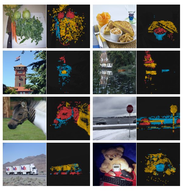
Figure 3: Attention maps from multiple heads. We consider the heads from the last layer of a ViT-S/8 trained with DINO and display the self-attention for [CLS] token query. Different heads, materialized by different colors, focus on different locations that represents different objects or parts (more examples in Appendix).
图 3:多头注意力图。 我们取用 DINO 训练的 ViT-S/8 最后一层各头,展示以 [CLS] token 为查询的自注意力。不同颜色表示不同头,关注代表不同物体或部件的不同位置(附录有更多例子)。
4.2.2 Discovering the semantic layout of scenes
As shown qualitatively in Figure 1, our self-attention maps contain information about the segmentation of an image. In this study, we measure this property on a standard benchmark as well as by directly probing the quality of masks generated from these attention maps.
4.2.2 发现场景的语义布局
如图 1 定性所示,我们的自注意力图包含图像分割信息。本研究在标准基准上度量该性质,并直接探测由这些注意力图生成的掩码质量。
Video instance segmentation.
In Tab. 5, we evaluate the output patch tokens on the DAVIS-2017 video instance segmentation benchmark [52]. We follow the experimental protocol in Jabri et al. [37] and segment scenes with a nearest-neighbor between consecutive frames; we thus do not train any model on top of the features, nor finetune any weights for the task. We observe in Tab. 5 that even though our training objective nor our architecture are designed for dense tasks, the performance is competitive on this benchmark. Since the network is not finetuned, the output of the model must have retained some spatial information. Finally, for this dense recognition task, the variants with small patches (“/8”) perform much better (+ & for ViT-B).
视频实例分割。
在表 5 中,我们在 DAVIS-2017 视频实例分割基准[52]上评估输出 patch token。遵循 Jabri 等[37]的实验协议,用连续帧之间的最近邻分割场景;因此不在特征上训练任何模型,也不为该任务微调权重。表 5 显示,尽管训练目标与架构都不是为稠密任务设计的,性能在该基准上仍有竞争力。由于网络未微调,模型输出必然保留了部分空间信息。对这一稠密识别任务,小 patch(“/8”)变体表现好得多(ViT-B 上 & 提升 +)。
Probing the self-attention map.
In Fig. 3, we show that different heads can attend to different semantic regions of an image, even when they are occluded (the bushes on the third row) or small (the flag on the second row). Visualizations are obtained with p images, resulting in sequences of 3601 tokens for ViT-S/8. In Fig. 4, we show that a supervised ViT does not attend well to objects in presence of clutter both qualitatively and quantitatively. We report the Jaccard similarity between the ground truth and segmentation masks obtained by thresholding the self-attention map to keep 60% of the mass. Note that the self-attention maps are smooth and not optimized to produce a mask. Nonetheless, we see a clear difference between the supervised or DINO models with a significant gap in terms of Jaccard similarities. Note that self-supervised convnets also contain information about segmentations but it requires dedicated methods to extract it from their weights [31].
探测自注意力图。
图 3 显示不同头可以关注图像的不同语义区域,即便被遮挡(第三行的灌木)或很小(第二行的旗帜)。可视化用 p 图像得到,对 ViT-S/8 形成 3601 个 token 的序列。图 4 表明有监督 ViT 在杂乱背景下无论定性还是定量都难以很好关注物体。我们报告把自注意力图阈值以保留 60% 质量后得到的分割掩码与真值之间的 Jaccard 相似度。注意自注意力图平滑,且并非为生成掩码而优化;尽管如此,有监督与 DINO 模型之间差异清晰,Jaccard 相似度差距显著。自监督卷积网络也包含分割信息,但需要专门方法从权重中提取[31]。
| Supervised | ||||
|---|---|---|---|---|
| DINO | ||||
| Random | Supervised | DINO | |
|---|---|---|---|
| ViT-S/16 | 22.0 | 27.3 | 45.9 |
| ViT-S/8 | 21.8 | 23.7 | 44.7 |
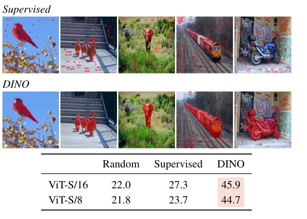
Figure 4: Segmentations from supervised versus DINO. We visualize masks obtained by thresholding the self-attention maps to keep 60% of the mass. On top, we show the resulting masks for a ViT-S/8 trained with supervision and DINO. We show the best head for both models. The table at the bottom compares the Jaccard similarity between the ground truth and these masks on the validation images of PASCAL VOC12 dataset.
| Supervised | ||||
|---|---|---|---|---|
| DINO | ||||
| Random | Supervised | DINO | |
|---|---|---|---|
| ViT-S/16 | 22.0 | 27.3 | 45.9 |
| ViT-S/8 | 21.8 | 23.7 | 44.7 |
图 4:有监督与 DINO 的分割。 可视化通过对自注意力图阈值、保留 60% 质量得到的掩码。上方展示用监督与 DINO 训练的 ViT-S/8 所得掩码;两边都展示最佳头。底表比较这些掩码与 PASCAL VOC12 验证集真值之间的 Jaccard 相似度。
4.2.3 Transfer learning on downstream tasks
In Tab. 6, we evaluate the quality of the features pretrained with DINO on different downstream tasks. We compare with features from the same architectures trained with supervision on ImageNet. We follow the protocol used in Touvron et al. [69] and finetune the features on each downstream task. We observe that for ViT architectures, self-supervised pretraining transfers better than features trained with supervision, which is consistent with observations made on convolutional networks [10, 33, 62]. Finally, self-supervised pretraining greatly improves results on ImageNet (+1-2%).
4.2.3 下游任务迁移学习
在表 6 中,我们评估用 DINO 预训练的特征在不同下游任务上的质量,并与同架构在 ImageNet 上有监督训练的特征比较。遵循 Touvron 等[69]的协议,在各下游任务上微调特征。可见对 ViT 架构,自监督预训练比有监督训练的特征迁移更好,这与卷积网络上的观察一致[10, 33, 62]。最后,自监督预训练在 ImageNet 上本身也显著提升结果(+1–2%)。
| Cifar | Cifar | INat | INat | Flwrs | Cars | INet | |
|---|---|---|---|---|---|---|---|
| ViT-S/16 | |||||||
| Sup. [69] | 99.0 | 89.5 | 70.7 | 76.6 | 98.2 | 92.1 | 79.9 |
| DINO | 99.0 | 90.5 | 72.0 | 78.2 | 98.5 | 93.0 | 81.5 |
| ViT-B/16 | |||||||
| Sup. [69] | 99.0 | 90.8 | 73.2 | 77.7 | 98.4 | 92.1 | 81.8 |
| DINO | 99.1 | 91.7 | 72.6 | 78.6 | 98.8 | 93.0 | 82.8 |
Table 6: Transfer learning by finetuning pretrained models on different datasets. We report top-1 accuracy. Self-supervised pretraining with DINO transfers better than supervised pretraining.
| Cifar | Cifar | INat | INat | Flwrs | Cars | INet | |
|---|---|---|---|---|---|---|---|
| ViT-S/16 | |||||||
| Sup. [69] | 99.0 | 89.5 | 70.7 | 76.6 | 98.2 | 92.1 | 79.9 |
| DINO | 99.0 | 90.5 | 72.0 | 78.2 | 98.5 | 93.0 | 81.5 |
| ViT-B/16 | |||||||
| Sup. [69] | 99.0 | 90.8 | 73.2 | 77.7 | 98.4 | 92.1 | 81.8 |
| DINO | 99.1 | 91.7 | 72.6 | 78.6 | 98.8 | 93.0 | 82.8 |
表 6:在不同数据集上微调预训练模型的迁移学习。 报告 top-1 准确率。用 DINO 做自监督预训练的迁移优于有监督预训练。
5 Ablation Study of DINO
5 DINO 消融研究
In this section, we empirically study DINO applied to ViT. The model considered for this entire study is ViT-S. We also refer the reader to Appendix for additional studies.
本节实证研究所应用在 ViT 上的 DINO。整节考虑的模型为 ViT-S。更多研究见附录。
5.1 Importance of the Different Components
5.1 不同组件的重要性
We show the impact of adding different components from self-supervised learning on ViT trained with our framework.
我们展示在我们的框架下训练 ViT 时,加入来自自监督学习的不同组件的影响。
| Method | Mom. | SK | MC | Loss | Pred. | -NN | Lin. | |
|---|---|---|---|---|---|---|---|---|
| 1 | DINO | ✓ | ✗ | ✓ | CE | ✗ | 72.8 | 76.1 |
| 2 | ✗ | ✗ | ✓ | CE | ✗ | 0.1 | 0.1 | |
| 3 | ✓ | ✓ | ✓ | CE | ✗ | 72.2 | 76.0 | |
| 4 | ✓ | ✗ | ✗ | CE | ✗ | 67.9 | 72.5 | |
| 5 | ✓ | ✗ | ✓ | MSE | ✗ | 52.6 | 62.4 | |
| 6 | ✓ | ✗ | ✓ | CE | ✓ | 71.8 | 75.6 | |
| 7 | BYOL | ✓ | ✗ | ✗ | MSE | ✓ | 66.6 | 71.4 |
| 8 | MoCov2 | ✓ | ✗ | ✗ | INCE | ✗ | 62.0 | 71.6 |
| 9 | SwAV | ✗ | ✓ | ✓ | CE | ✗ | 64.7 | 71.8 |
| SK: Sinkhorn-Knopp, MC: Multi-Crop, Pred.: Predictor | ||||||||
| CE: Cross-Entropy, MSE: Mean Square Error, INCE: InfoNCE |
Table 7: Important component for self-supervised ViT pretraining. Models are trained for 300 epochs with ViT-S/16. We study the different components that matter for the -NN and linear (“Lin.”) evaluations. For the different variants, we highlight the differences from the default DINO setting. The best combination is the momentum encoder with the multicrop augmentation and the cross-entropy loss. We also report results with BYOL [30], MoCo-v2 [15] and SwAV [10].
| Method | Mom. | SK | MC | Loss | Pred. | -NN | Lin. | |
|---|---|---|---|---|---|---|---|---|
| 1 | DINO | ✓ | ✗ | ✓ | CE | ✗ | 72.8 | 76.1 |
| 2 | ✗ | ✗ | ✓ | CE | ✗ | 0.1 | 0.1 | |
| 3 | ✓ | ✓ | ✓ | CE | ✗ | 72.2 | 76.0 | |
| 4 | ✓ | ✗ | ✗ | CE | ✗ | 67.9 | 72.5 | |
| 5 | ✓ | ✗ | ✓ | MSE | ✗ | 52.6 | 62.4 | |
| 6 | ✓ | ✗ | ✓ | CE | ✓ | 71.8 | 75.6 | |
| 7 | BYOL | ✓ | ✗ | ✗ | MSE | ✓ | 66.6 | 71.4 |
| 8 | MoCov2 | ✓ | ✗ | ✗ | INCE | ✗ | 62.0 | 71.6 |
| 9 | SwAV | ✗ | ✓ | ✓ | CE | ✗ | 64.7 | 71.8 |
| SK:Sinkhorn-Knopp,MC:Multi-Crop,Pred.:预测器 | ||||||||
| CE:交叉熵,MSE:均方误差,INCE:InfoNCE |
表 7:自监督 ViT 预训练的关键组件。 模型用 ViT-S/16 训练 300 个 epoch。我们研究对 -NN 与线性(“Lin.”)评估重要的不同组件。对各变体,标出相对默认 DINO 设定的差异。最佳组合是动量编码器配合 multicrop 增强与交叉熵损失。也报告 BYOL[30]、MoCo-v2[15] 与 SwAV[10] 的结果。
In Table 7, we report different model variants as we add or remove components. First, we observe that in the absence of momentum, our framework does not work (row 2) and more advanced operations, SK for example, are required to avoid collapse (row 9). However, with momentum, using SK has little impact (row 3). In addtition, comparing rows 3 and 9 highlights the importance of the momentum encoder for performance. Second, in rows 4 and 5, we observe that multi-crop training and the cross-entropy loss in DINO are important components to obtain good features. We also observe that adding a predictor to the student network has little impact (row 6) while it is critical in BYOL to prevent collapse [16, 30]. For completeness, we propose in Appendix B an extended version of this ablation study.
表 7 报告增删组件后的不同模型变体。首先,没有动量时本框架无法工作(第 2 行),需要更高级操作(例如 SK)才能避免崩塌(第 9 行)。但有动量时,使用 SK 影响很小(第 3 行)。比较第 3 与第 9 行还突出了动量编码器对性能的重要性。其次,第 4、5 行显示 multi-crop 训练与 DINO 中的交叉熵损失是获得良好特征的重要组件。我们也观察到给学生网络加预测器影响很小(第 6 行),而这在 BYOL 中对防止崩塌至关重要[16, 30]。为完整起见,附录 B 给出本消融的扩展版本。
Importance of the patch size.
In Fig. 5, we compare the -NN classification performance of ViT-S models trained with different patch sizes, , and . We also compare to ViT-B with and patches. All the models are trained for 300 epochs. We observe that the performance greatly improves as we decrease the size of the patch. It is interesting to see that performance can be greatly improved without adding additional parameters. However, the performance gain from using smaller patches comes at the expense of throughput: when using 55 patches, the throughput falls to 44 im/s, vs 180 im/s for 88 patches.
patch 大小的重要性。
图 5 比较用不同 patch 大小 、 与 训练的 ViT-S 的 -NN 分类性能,并与 、 patch 的 ViT-B 比较。所有模型训练 300 个 epoch。可见随 patch 变小,性能显著提升。有趣的是,无需增加参数即可大幅提升性能。但小 patch 的收益以吞吐为代价:使用 55 patch 时吞吐降至 44 im/s,而 88 patch 为 180 im/s。
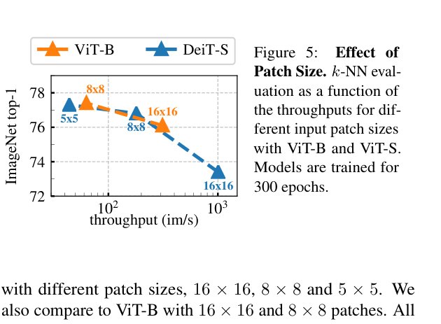
Figure 5: Effect of Patch Size. -NN evaluation as a function of the throughputs for different input patch sizes with ViT-B and ViT-S. Models are trained for 300 epochs.
图 5:Patch 大小的影响。 对不同输入 patch 大小的 ViT-B 与 ViT-S,以吞吐为函数的 -NN 评估。模型训练 300 个 epoch。
5.2 Impact of the choice of Teacher Network
5.2 教师网络选择的影响
In this ablation, we experiment with different teacher network to understand its role in DINO. We compare models trained for epochs using the -NN protocol.
本消融试验不同教师网络以理解其在 DINO 中的作用。比较用 -NN 协议训练 个 epoch 的模型。
Building different teachers from the student.
In Fig. 6(right), we compare different strategies to build the teacher from previous instances of the student besides the momentum teacher. First we consider using the student network from a previous epoch as a teacher. This strategy has been used in a memory bank [73] or as a form of clustering hard-distillation [8, 2, 14]. Second, we consider using the student network from the previous iteration, as well as a copy of the student for the teacher. In our setting, using a teacher based on a recent version of the student does not converge. This setting requires more normalizations to work. Interestingly, we observe that using a teacher from the previous epoch does not collapse, providing performance in the -NN evaluation competitive with existing frameworks such as MoCo-v2 or BYOL. While using a momentum encoder clearly provides superior performance to this naive teacher, this finding suggests that there is a space to investigate alternatives for the teacher.
从学生构建不同教师。
图 6(右)比较除动量教师外、用学生历史实例构建教师的不同策略。首先考虑用上一 epoch 的学生网络作教师;该策略曾用于记忆库[73]或作为聚类硬蒸馏的一种形式[8, 2, 14]。其次考虑用上一迭代的学生网络,以及学生的副本作教师。在我们设定中,基于学生近期版本的教师无法收敛,需要更多归一化才能工作。有趣的是,用上一 epoch 的教师不会崩塌,在 -NN 评估上可与 MoCo-v2 或 BYOL 等现有框架竞争。尽管动量编码器明显优于这种朴素教师,这一发现表明教师仍有其他可探索的替代方案。
Analyzing the training dynamic.
To further understand the reasons why a momentum teacher works well in our framework, we study its dynamic during the training of a ViT in the left panel of Fig. 6. A key observation is that this teacher constantly outperforms the student during the training, and we observe the same behavior when training with a ResNet-50 (Appendix D). This behavior has not been observed by other frameworks also using momentum [33, 30], nor when the teacher is built from the previous epoch. We propose to interpret the momentum teacher in DINO as a form of Polyak-Ruppert averaging [51, 59] with an exponentially decay. Polyak-Ruppert averaging is often used to simulate model ensembling to improve the performance of a network at the end of the training [38]. Our method can be interpreted as applying Polyak-Ruppert averaging during the training to constantly build a model ensembling that has superior performances. This model ensembling then guides the training of the student network [65].
分析训练动态。
为进一步理解动量教师在本框架中为何有效,我们在图 6 左图研究其在 ViT 训练中的动态。关键观察是:该教师在训练全程持续优于学生;用 ResNet-50 训练时也看到同样行为(附录 D)。使用动量的其他框架[33, 30]以及由上一 epoch 构建教师时均未观察到这一行为。我们提议把 DINO 中的动量教师解释为带指数衰减的 Polyak-Ruppert 平均[51, 59]。Polyak-Ruppert 平均常用于在训练结束时模拟模型集成以提升网络性能[38]。我们的方法可理解为在训练过程中持续应用 Polyak-Ruppert 平均,不断构建性能更优的模型集成,再由该集成引导学生网络训练[65]。
| Teacher | Top-1 |
|---|---|
| Student copy | 0.1 |
| Previous iter | 0.1 |
| Previous epoch | 66.6 |
| Momentum | 72.8 |
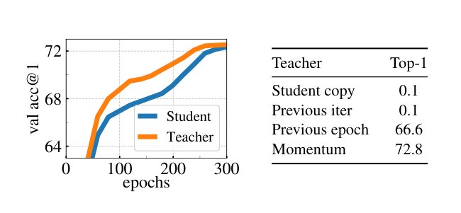
Figure 6: Top-1 accuracy on ImageNet validation with -NN classifier. (left) Comparison between the performance of the momentum teacher and the student during training. (right) Comparison between different types of teacher network. The momentum encoder leads to the best performance but is not the only viable option.
| Teacher | Top-1 |
|---|---|
| Student copy | 0.1 |
| Previous iter | 0.1 |
| Previous epoch | 66.6 |
| Momentum | 72.8 |
图 6:ImageNet 验证集上用 -NN 分类器的 Top-1 准确率。(左) 训练过程中动量教师与学生性能比较。(右) 不同类型教师网络比较。动量编码器效果最好,但并非唯一可行选项。
5.3 Avoiding collapse
5.3 避免崩塌
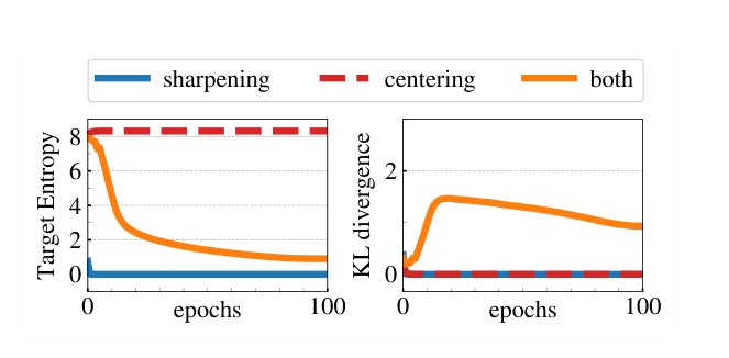
Figure 7: Collapse study. (left): evolution of the teacher’s target entropy along training epochs; (right): evolution of KL divergence between teacher and student outputs.
图 7:崩塌研究。(左):训练 epoch 上教师目标熵的演化;(右):教师与学生输出之间 KL 散度的演化。
We study the complementarity role of centering and target sharpening to avoid collapse. There are two forms of collapse: regardless of the input, the model output is uniform along all the dimensions or dominated by one dimension. The centering avoids the collapse induced by a dominant dimension, but encourages an uniform output. Sharpening induces the opposite effect. We show this complementarity by decomposing the cross-entropy into an entropy and the Kullback-Leibler divergence (“KL”) :
我们研究中心化与目标锐化在避免崩塌上的互补作用。崩塌有两种形式:不论输入如何,模型输出在所有维上均匀,或由某一维主导。中心化避免由主导维引起的崩塌,但鼓励均匀输出;锐化则相反。我们通过把交叉熵 分解为熵 与 Kullback-Leibler 散度(“KL”) 来展示这种互补:
A KL equal to zero indicates a constant output, and hence a collapse. In Fig. 7, we plot the entropy and KL during training with and without centering and sharpening. If one operation is missing, the KL converges to zero, indicating a collapse. However, the entropy converges to different values: with no centering and with no sharpening, indicating that both operations induce different form of collapse. Applying both operations balances these effects (see study of the sharpening parameter in Appendix D).
KL 等于零表示输出恒定,因而发生崩塌。图 7 绘制有无中心化与锐化时训练过程中的熵与 KL。若缺少任一操作,KL 收敛到零,表明崩塌。但熵 收敛到不同值:无中心化时为 ,无锐化时为 ,表明两种操作诱发不同形式的崩塌。两者并用可平衡这些效应(锐化参数 的研究见附录 D)。
5.4 Compute requirements
5.4 计算需求
| 100 epochs | 300 epochs | ||||||
|---|---|---|---|---|---|---|---|
| multi-crop | top-1 | time | top-1 | time | mem. | ||
| 67.8 | 15.3h | 72.5 | 45.9h | 9.3G | |||
| 71.5 | 17.0h | 74.5 | 51.0h | 10.5G | |||
| 73.8 | 20.3h | 75.9 | 60.9h | 12.9G | |||
| 74.6 | 24.2h | 76.1 | 72.6h | 15.4G |
Table 8: Time and memory requirements. We show total running time and peak memory per GPU (“mem.”) when running ViT-S/16 DINO models on two 8-GPU machines. We report top-1 ImageNet val acc with linear evaluation for several variants of multi-crop, each having a different level of compute requirement.
| 100 epochs | 300 epochs | ||||||
|---|---|---|---|---|---|---|---|
| multi-crop | top-1 | time | top-1 | time | mem. | ||
| 67.8 | 15.3h | 72.5 | 45.9h | 9.3G | |||
| 71.5 | 17.0h | 74.5 | 51.0h | 10.5G | |||
| 73.8 | 20.3h | 75.9 | 60.9h | 12.9G | |||
| 74.6 | 24.2h | 76.1 | 72.6h | 15.4G |
表 8:时间与显存需求。 展示在两台 8-GPU 机器上运行 ViT-S/16 DINO 模型时的总运行时间与每 GPU 峰值显存(“mem.”)。报告若干 multi-crop 变体在线性评估下的 ImageNet 验证 top-1,各变体计算需求不同。
In Tab. 8, we detail the time and GPU memory requirements when running ViT-S/16 DINO models on two -GPU machines. We report results with several variants of multi-crop training, each having a different level of compute requirement. We observe in Tab. 8 that using multi-crop improves the accuracy / running-time tradeoff for DINO runs. For example, the performance is after hours of training without multi-crop (i.e. ) while DINO in crop setting reaches in hours only. This is an improvement of while requiring less time, though the memory usage is higher ( versus ). We observe that the performance boost brought with multi-crop cannot be caught up by more training in the setting, which shows the value of the “local-to-global” augmentation. Finally, the gain from adding more views diminishes (+.2% form to crops) for longer trainings.
表 8 详列在两台 -GPU 机器上运行 ViT-S/16 DINO 模型的时间与 GPU 显存需求,并报告若干不同计算量的 multi-crop 训练变体结果。可见 multi-crop 改善了 DINO 运行的准确率/运行时间权衡。例如,无 multi-crop(即 )训练 46 小时后性能为 ,而 设定下仅 24 小时即达 :提升 同时时间约减半,尽管显存更高( 对 )。我们观察到 multi-crop 带来的提升无法被 设定下更长训练追上,说明“局部到全局”增强的价值。最后,增加更多视图的收益递减(从 到 个 裁剪,长训仅 +.2%)。
Overall, training DINO with Vision Transformers achieves top-1 accuracy using two 8-GPU servers for 3 days. This result outperforms state-of-the-art self-supervised systems based on convolutional networks of comparable sizes with a significant reduction of computational requirements [30, 10]. Our code is available to train self-supervised ViT on a limited number of GPUs.
总体而言,用 Vision Transformer 训练 DINO,两台 8-GPU 服务器运行 3 天即可达到 top-1 准确率。该结果优于同规模卷积网络上的当时最优自监督系统,且计算需求显著降低[30, 10]。
5.5 Training with small batches
5.5 小批次训练
| bs | 128 | 256 | 512 | 1024 |
|---|---|---|---|---|
| top-1 | 57.9 | 59.1 | 59.6 | 59.9 |
Table 9: Effect of batch sizes. Top-1 with -NN for models trained for 100 epochs without multi-crop.
| bs | 128 | 256 | 512 | 1024 |
|---|---|---|---|---|
| top-1 | 57.9 | 59.1 | 59.6 | 59.9 |
表 9:批次大小的影响。 无 multi-crop、训练 100 个 epoch 的模型的 -NN Top-1。
In Tab. 9, we study the impact of the batch size on the features obtained with DINO. We also study the impact of the smooth parameter used in the centering update rule of Eq. 4 in Appendix D. We scale the learning rate linearly with the batch size [29]: . Tab. 9 confirms that we can train models to high performance with small batches. Results with the smaller batch sizes () are slightly below our default training setup of , and would certainly require to re-tune hyperparameters like the momentum rates for example. Note that the experiment with batch size of runs on only GPU. We have explored training a model with a batch size of , reaching after epochs, showing the potential for training large models that barely fit an image per GPU.
表 9 研究批次大小对 DINO 所得特征的影响。式 (4) 中心化更新规则中平滑参数 的影响见附录 D。学习率随批次大小线性缩放[29]:。表 9 证实可用小批次把模型训到高性能。较小批次()的结果略低于默认 设定,肯定需要重新调诸如动量系数等超参。注意 的实验只在 张 GPU 上运行。我们还探索过 的训练,50 个 epoch 后达到 ,显示了训练几乎每 GPU 只能放一张图的大模型的潜力。
6 Conclusion
6 结论
In this work, we have shown the potential of self-supervised pretraining a standard ViT model, achieving performance that are comparable with the best convnets specifically designed for this setting. We have also seen emerged two properties that can be leveraged in future applications: the quality of the features in -NN classification has a potential for image retrieval where ViT are already showing promising results [22]. The presence of information about the scene layout in the features can also benefit weakly supervised image segmentation. However, the main result of this paper is that we have evidences that self-supervised learning could be the key to developing a BERT-like model based on ViT. In the future, we plan to explore if pretraining a large ViT model with DINO on random uncurated images could push the limits of visual features [28].
本工作展示了用标准 ViT 做自监督预训练的潜力,性能可与专为该设定设计的最佳卷积网络相当。我们还看到两种可在未来应用中利用的涌现性质:-NN 分类中特征的质量有望用于图像检索——ViT 在该方向已有可喜结果[22];特征中包含的场景布局信息也可惠及弱监督图像分割。然而本文主要结果是:有证据表明自监督学习可能是开发基于 ViT 的类 BERT 模型的关键。未来我们计划探索:用 DINO 在随机、未经策展的图像上预训练大型 ViT,能否推高视觉特征的上限[28]。
Acknowledgement.
We thank Mahmoud Assran, Matthijs Douze, Allan Jabri, Jure Zbontar, Alaaeldin El-Nouby, Y-Lan Boureau, Kaiming He, Thomas Lucas as well as the Thoth and FAIR teams for their help, support and discussions around this project. Julien Mairal was funded by the ERC grant number 714381 (SOLARIS project) and by ANR 3IA MIAI@Grenoble Alpes (ANR-19-P3IA-0003).
致谢。
感谢 Mahmoud Assran、Matthijs Douze、Allan Jabri、Jure Zbontar、Alaaeldin El-Nouby、Y-Lan Boureau、Kaiming He、Thomas Lucas 以及 Thoth 与 FAIR 团队对本项目的帮助、支持与讨论。Julien Mairal 受 ERC 资助号 714381(SOLARIS 项目)以及 ANR 3IA MIAI@Grenoble Alpes(ANR-19-P3IA-0003)资助。
References
参考文献
[1] Rohan Anil, Gabriel Pereyra, Alexandre Passos, Robert Ormandi, George E Dahl, and Geoffrey E Hinton. Large scale distributed neural network training through online distillation. arXiv preprint arXiv:1804.03235 , 2018.
[2] Yuki Markus Asano, Christian Rupprecht, and Andrea Vedaldi. Self-labelling via simultaneous clustering and representation learning. In ICLR , 2020.
[3] Mahmoud Assran, Nicolas Ballas, Lluis Castrejon, and Michael Rabbat. Recovering petaflops in contrastive semi-supervised learning of visual representations. preprint arXiv:2006.10803 , 2020.
[4] Dzmitry Bahdanau, Kyunghyun Cho, and Yoshua Bengio. Neural machine translation by jointly learning to align and translate. preprint arXiv:1409.0473 , 2014.
[5] Maxim Berman, Hervé Jégou, Vedaldi Andrea, Iasonas Kokkinos, and Matthijs Douze. MultiGrain: a unified image embedding for classes and instances. arXiv preprint arXiv:1902.05509 , 2019.
[6] Piotr Bojanowski and Armand Joulin. Unsupervised learning by predicting noise. In ICML , 2017.
[7] Cristian Buciluǎ, Rich Caruana, and Alexandru Niculescu-Mizil. Model compression. In SIGKDD , 2006.
[8] Mathilde Caron, Piotr Bojanowski, Armand Joulin, and Matthijs Douze. Deep clustering for unsupervised learning of visual features. In ECCV , 2018.
[9] Mathilde Caron, Piotr Bojanowski, Julien Mairal, and Armand Joulin. Unsupervised pre-training of image features on non-curated data. In ICCV , 2019.
[10] Mathilde Caron, Ishan Misra, Julien Mairal, Priya Goyal, Piotr Bojanowski, and Armand Joulin. Unsupervised learning of visual features by contrasting cluster assignments. In NeurIPS , 2020.
[11] Mia Xu Chen, Orhan Firat, Ankur Bapna, Melvin Johnson, Wolfgang Macherey, George Foster, Llion Jones, Niki Parmar, Mike Schuster, Zhifeng Chen, et al. The best of both worlds: Combining recent advances in neural machine translation. preprint arXiv:1804.09849 , 2018.
[12] Ting Chen, Simon Kornblith, Mohammad Norouzi, and Geoffrey Hinton. A simple framework for contrastive learning of visual representations. preprint arXiv:2002.05709 , 2020.
[13] Ting Chen, Simon Kornblith, Kevin Swersky, Mohammad Norouzi, and Geoffrey Hinton. Big self-supervised models are strong semi-supervised learners. In NeurIPS , 2020.
[14] Weijie Chen, Shiliang Pu, Di Xie, Shicai Yang, Yilu Guo, and Luojun Lin. Unsupervised image classification for deep representation learning. arXiv preprint arXiv:2006.11480 , 2020.
[15] Xinlei Chen, Haoqi Fan, Ross Girshick, and Kaiming He. Improved baselines with momentum contrastive learning. preprint arXiv:2003.04297 , 2020.
[16] Xinlei Chen and Kaiming He. Exploring simple siamese representation learning. preprint arXiv:2011.10566 , 2020.
[17] Marco Cuturi. Sinkhorn distances: Lightspeed computation of optimal transport. In NeurIPS , 2013.
[18] Jacob Devlin, Ming-Wei Chang, Kenton Lee, and Kristina Toutanova. Bert: Pre-training of deep bidirectional transformers for language understanding. preprint arXiv:1810.04805 , 2018.
[19] Alexey Dosovitskiy, Lucas Beyer, Alexander Kolesnikov, Dirk Weissenborn, Xiaohua Zhai, Thomas Unterthiner, Mostafa Dehghani, Matthias Minderer, Georg Heigold, Sylvain Gelly, et al. An image is worth 16x16 words: Transformers for image recognition at scale. preprint arXiv:2010.11929 , 2020.
[20] Alexey Dosovitskiy, Philipp Fischer, Jost Tobias Springenberg, Martin Riedmiller, and Thomas Brox. Discriminative unsupervised feature learning with exemplar convolutional neural networks. TPAMI , 2016.
[21] Matthijs Douze, Hervé Jégou, Harsimrat Sandhawalia, Laurent Amsaleg, and Cordelia Schmid. Evaluation of gist descriptors for web-scale image search. In CIVR , 2009.
[22] Alaaeldin El-Nouby, Natalia Neverova, Ivan Laptev, and Hervé Jégou. Training vision transformers for image retrieval. preprint arXiv:2102.05644 , 2021.
[23] Aleksandr Ermolov, Aliaksandr Siarohin, Enver Sangineto, and Nicu Sebe. Whitening for self-supervised representation learning. preprint arXiv:2007.06346 , 2020.
[24] Mark Everingham, Luc Van Gool, Christopher KI Williams, John Winn, and Andrew Zisserman. The pascal visual object classes (voc) challenge. IJCV , 2010.
[25] Zhiyuan Fang, Jianfeng Wang, Lijuan Wang, Lei Zhang, Yezhou Yang, and Zicheng Liu. Seed: Self-supervised distillation for visual representation. 2021.
[26] Spyros Gidaris, Andrei Bursuc, Nikos Komodakis, Patrick Pérez, and Matthieu Cord. Learning representations by predicting bags of visual words. In CVPR , 2020.
[27] Spyros Gidaris, Andrei Bursuc, Gilles Puy, Nikos Komodakis, Matthieu Cord, and Patrick Pérez. Online bag-of-visual-words generation for unsupervised representation learning. arXiv preprint arXiv:2012.11552 , 2020.
[28] Priya Goyal, Mathilde Caron, Benjamin Lefaudeux, Min Xu, Pengchao Wang, Vivek Pai, Mannat Singh, Vitaliy Liptchinsky, Ishan Misra, Armand Joulin, et al. Self-supervised pretraining of visual features in the wild. preprint arXiv:2103.01988 , 2021.
[29] Priya Goyal, Piotr Dollár, Ross Girshick, Pieter Noordhuis, Lukasz Wesolowski, Aapo Kyrola, Andrew Tulloch, Yangqing Jia, and Kaiming He. Accurate, large minibatch sgd: Training imagenet in 1 hour. preprint arXiv:1706.02677 , 2017.
[30] Jean-Bastien Grill, Florian Strub, Florent Altché, Corentin Tallec, Pierre H Richemond, Elena Buchatskaya, Carl Doersch, Bernardo Avila Pires, Zhaohan Daniel Guo, Mohammad Gheshlaghi Azar, Bilal Piot, Koray Kavukcuoglu, Rémi Munos, and Michal Valko. Bootstrap your own latent: A new approach to self-supervised learning. In NeurIPS , 2020.
[31] Shir Gur, Ameen Ali, and Lior Wolf. Visualization of supervised and self-supervised neural networks via attribution guided factorization. preprint arXiv:2012.02166 , 2020.
[32] Michael Gutmann and Aapo Hyvärinen. Noise-contrastive estimation: A new estimation principle for unnormalized statistical models. In International Conference on Artificial Intelligence and Statistics , 2010.
[33] Kaiming He, Haoqi Fan, Yuxin Wu, Saining Xie, and Ross Girshick. Momentum contrast for unsupervised visual representation learning. In CVPR , 2020.
[34] Kaiming He, Xiangyu Zhang, Shaoqing Ren, and Jian Sun. Deep residual learning for image recognition. In CVPR , 2016.
[35] Geoffrey Hinton, Oriol Vinyals, and Jeff Dean. Distilling the knowledge in a neural network. preprint arXiv:1503.02531 , 2015.
[36] Jiabo Huang, Qi Dong, Shaogang Gong, and Xiatian Zhu. Unsupervised deep learning by neighbourhood discovery. In ICML , 2019.
[37] Allan Jabri, Andrew Owens, and Alexei A Efros. Space-time correspondence as a contrastive random walk. 2020.
[38] Sébastien Jean, Kyunghyun Cho, Roland Memisevic, and Yoshua Bengio. On using very large target vocabulary for neural machine translation. preprint arXiv:1412.2007 , 2014.
[39] Guillaume Klein, Yoon Kim, Yuntian Deng, Jean Senellart, and Alexander M Rush. Opennmt: Open-source toolkit for neural machine translation. preprint arXiv:1701.02810 , 2017.
[40] Zihang Lai, Erika Lu, and Weidi Xie. Mast: A memory-augmented self-supervised tracker. In CVPR , 2020.
[41] Dong-Hyun Lee et al. Pseudo-label: The simple and efficient semi-supervised learning method for deep neural networks. In Workshop on challenges in representation learning, ICML , 2013.
[42] Junnan Li, Pan Zhou, Caiming Xiong, and Steven C.H. Hoi. Prototypical contrastive learning of unsupervised representations. ICLR , 2021.
[43] Ilya Loshchilov and Frank Hutter. Sgdr: Stochastic gradient descent with warm restarts. preprint arXiv:1608.03983 , 2016.
[44] Ilya Loshchilov and Frank Hutter. Fixing weight decay regularization in adam. 2018.
[45] Julien Mairal. Cyanure: An open-source toolbox for empirical risk minimization for python, c++, and soon more. preprint arXiv:1912.08165 , 2019.
[46] Maria-Elena Nilsback and Andrew Zisserman. Automated flower classification over a large number of classes. In 2008 Sixth Indian Conference on Computer Vision, Graphics & Image Processing , 2008.
[47] Mehdi Noroozi, Ananth Vinjimoor, Paolo Favaro, and Hamed Pirsiavash. Boosting self-supervised learning via knowledge transfer. In CVPR , 2018.
[48] Seoung Wug Oh, Joon-Young Lee, Ning Xu, and Seon Joo Kim. Video object segmentation using space-time memory networks. In ICCV , 2019.
[49] Hieu Pham, Qizhe Xie, Zihang Dai, and Quoc V Le. Meta pseudo labels. preprint arXiv:2003.10580 , 2020.
[50] James Philbin, Ondrej Chum, Michael Isard, Josef Sivic, and Andrew Zisserman. Lost in quantization: Improving particular object retrieval in large scale image databases. In CVPR , 2008.
[51] Boris T Polyak and Anatoli B Juditsky. Acceleration of stochastic approximation by averaging. SIAM journal on control and optimization , 30(4):838–855, 1992.
[52] Jordi Pont-Tuset, Federico Perazzi, Sergi Caelles, Pablo Arbeláez, Alex Sorkine-Hornung, and Luc Van Gool. The 2017 davis challenge on video object segmentation. preprint arXiv:1704.00675 , 2017.
[53] Filip Radenović, Ahmet Iscen, Giorgos Tolias, Yannis Avrithis, and Ondřej Chum. Revisiting oxford and paris: Large-scale image retrieval benchmarking. 2018.
[54] Filip Radenović, Giorgos Tolias, and Ondřej Chum. Fine-tuning cnn image retrieval with no human annotation. IEEE transactions on pattern analysis and machine intelligence , 2018.
[55] Alec Radford, Jeffrey Wu, Rewon Child, David Luan, Dario Amodei, and Ilya Sutskever. Language models are unsupervised multitask learners.
[56] Ilija Radosavovic, Raj Prateek Kosaraju, Ross Girshick, Kaiming He, and Piotr Dollár. Designing network design spaces. In CVPR , 2020.
[57] Jerome Revaud, Jon Almazán, Rafael S Rezende, and Cesar Roberto de Souza. Learning with average precision: Training image retrieval with a listwise loss. In ICCV , 2019.
[58] Pierre H Richemond, Jean-Bastien Grill, Florent Altché, Corentin Tallec, Florian Strub, Andrew Brock, Samuel Smith, Soham De, Razvan Pascanu, Bilal Piot, et al. Byol works even without batch statistics. preprint arXiv:2010.10241 , 2020.
[59] David Ruppert. Efficient estimations from a slowly convergent robbins-monro process. Technical report, 1988.
[60] Olga Russakovsky, Jia Deng, Hao Su, Jonathan Krause, Sanjeev Satheesh, Sean Ma, Zhiheng Huang, Andrej Karpathy, Aditya Khosla, Michael Bernstein, Alexander C Berg, and Li Fei-Fei. Imagenet large scale visual recognition challenge. IJCV , 2015.
[61] Tim Salimans and Diederik P Kingma. Weight normalization: A simple reparameterization to accelerate training of deep neural networks. NeurIPS , 2016.
[62] Mert Bulent Sariyildiz, Yannis Kalantidis, Diane Larlus, and Karteek Alahari. Concept generalization in visual representation learning. arXiv preprint arXiv:2012.05649 , 2020.
[63] Zhiqiang Shen, Zechun Liu, Jie Qin, Lei Huang, Kwang-Ting Cheng, and Marios Savvides. S2-bnn: Bridging the gap between self-supervised real and 1-bit neural networks via guided distribution calibration. arXiv preprint arXiv:2102.08946 , 2021.
[64] Kihyuk Sohn, David Berthelot, Chun-Liang Li, Zizhao Zhang, Nicholas Carlini, Ekin D Cubuk, Alex Kurakin, Han Zhang, and Colin Raffel. Fixmatch: Simplifying semi-supervised learning with consistency and confidence. In NeurIPS , 2020.
[65] Antti Tarvainen and Harri Valpola. Mean teachers are better role models: Weight-averaged consistency targets improve semi-supervised deep learning results. preprint arXiv:1703.01780 , 2017.
[66] Bart Thomee, David A Shamma, Gerald Friedland, Benjamin Elizalde, Karl Ni, Douglas Poland, Damian Borth, and Li-Jia Li. Yfcc100m: The new data in multimedia research. arXiv preprint arXiv:1503.01817 , 2015.
[67] Yonglong Tian, Chen Sun, Ben Poole, Dilip Krishnan, Cordelia Schmid, and Phillip Isola. What makes for good views for contrastive learning. NeurIPS , 2020.
[68] Giorgos Tolias, Ronan Sicre, and Hervé Jégou. Particular object retrieval with integral max-pooling of cnn activations. arXiv preprint arXiv:1511.05879 , 2015.
[69] Hugo Touvron, Matthieu Cord, Matthijs Douze, Francisco Massa, Alexandre Sablayrolles, and Hervé Jégou. Training data-efficient image transformers & distillation through attention. preprint arXiv:2012.12877 , 2020.
[70] Ashish Vaswani, Noam Shazeer, Niki Parmar, Jakob Uszkoreit, Llion Jones, Aidan N Gomez, Łukasz Kaiser, and Illia Polosukhin. Attention is all you need. In NeurIPS , 2017.
[71] Xiaolong Wang, Allan Jabri, and Alexei A Efros. Learning correspondence from the cycle-consistency of time. In CVPR , 2019.
[72] Tobias Weyand, Andre Araujo, Bingyi Cao, and Jack Sim. Google landmarks dataset v2-a large-scale benchmark for instance-level recognition and retrieval. 2020.
[73] Zhirong Wu, Yuanjun Xiong, Stella X Yu, and Dahua Lin. Unsupervised feature learning via non-parametric instance discrimination. In CVPR , 2018.
[74] Junyuan Xie, Ross Girshick, and Ali Farhadi. Unsupervised deep embedding for clustering analysis. In ICML , 2016.
[75] Qizhe Xie, Zihang Dai Dai, Eduard Hovy, Minh-Thang Luong, and Quoc V. Le. Unsupervised data augmentation for consistency training. preprint arXiv:1904.12848 , 2020.
[76] Qizhe Xie, Minh-Thang Luong, Eduard Hovy, and Quoc V Le. Self-training with noisy student improves imagenet classification. In CVPR , 2020.
[77] Haohang Xu, Xiaopeng Zhang, Hao Li, Lingxi Xie, Hongkai Xiong, and Qi Tian. Seed the views: Hierarchical semantic alignment for contrastive representation learning. arXiv preprint arXiv:2012.02733 , 2021.
[78] Qiantong Xu, Tatiana Likhomanenko, Jacob Kahn, Awni Hannun, Gabriel Synnaeve, and Ronan Collobert. Iterative pseudo-labeling for speech recognition. preprint arXiv:2005.09267 , 2020.
[79] I Zeki Yalniz, Hervé Jégou, Kan Chen, Manohar Paluri, and Dhruv Mahajan. Billion-scale semi-supervised learning for image classification. preprint arXiv:1905.00546 , 2019.
[80] Jianwei Yang, Devi Parikh, and Dhruv Batra. Joint unsupervised learning of deep representations and image clusters. In CVPR , 2016.
[81] Jure Zbontar, Li Jing, Ishan Misra, Yann LeCun, and Stéphane Deny. Barlow twins: Self-supervised learning via redundancy reduction. arXiv preprint arXiv:2103.03230 , 2021.
[82] Richard Zhang, Phillip Isola, and Alexei A Efros. Colorful image colorization. In ECCV , 2016.
[83] Hengshuang Zhao, Jiaya Jia, and Vladlen Koltun. Exploring self-attention for image recognition. In CVPR , 2020.
[84] Bolei Zhou, Agata Lapedriza, Jianxiong Xiao, Antonio Torralba, and Aude Oliva. Learning deep features for scene recognition using places database. In NeurIPS , 2014.
[85] Chengxu Zhuang, Alex Lin Zhai, and Daniel Yamins. Local aggregation for unsupervised learning of visual embeddings. In ICCV , 2019.
Appendix
附录
A Additional Results
A 补充结果
-NN classification.
In Tab. 10, we evaluate the frozen representations given by ResNet-50 or ViT-small pre-trained with DINO with two evaluation protocols: linear or -NN. For both evaluations, we extract representations from a pre-trained network without using any data augmentation. Then, we perform classification either with weighted -NN or with a linear regression learned with cyanure library [45]. In Tab. 10 we see that ViT-S accuracies are better than accuracies obtained with RN50 both with a linear or a -NN classifier. However, the performance gap when using the -NN evaluation is much more significant than when considering linear evaluation. For example on ImageNet 1%, ViT-S outperforms ResNet-50 by a large margin of with -NN evaluation. This suggests that transformers architectures trained with DINO might offer more model flexibility that benefits the -NN evaluation. -NN classifiers have the great advantage of being fast and light to deploy, without requiring any domain adaptation. Overall, ViT trained with DINO provides features that combine particularly well with -NN classifiers.
-NN 分类。
表 10 用线性或 -NN 两种协议评估用 DINO 预训练的 ResNet-50 或 ViT-small 的冻结表征。两种评估都不使用数据增强,从预训练网络提取表征;再用加权 -NN 或用 cyanure 库[45]学习的线性回归做分类。表 10 显示:无论线性还是 -NN 分类器,ViT-S 准确率都高于 RN50;但 -NN 评估下的性能差距远大于线性评估。例如在 ImageNet 1% 上,ViT-S 用 -NN 评估大幅超过 ResNet-50(+)。这表明用 DINO 训练的 Transformer 架构可能提供更有利于 -NN 评估的模型灵活性。-NN 分类器部署快、轻量,无需域适配。总体而言,用 DINO 训练的 ViT 提供的特征与 -NN 分类器特别合拍。
| Logistic | -NN | ||||||
|---|---|---|---|---|---|---|---|
| RN50 | ViT-S | RN50 | ViT-S | ||||
| Inet 100% | 72.1 | 75.7 | 3.6 | 67.5 | 74.5 | 7.0 | |
| Inet 10% | 67.8 | 72.2 | 4.4 | 59.3 | 69.1 | 9.8 | |
| Inet 1% | 55.1 | 64.5 | 9.4 | 47.2 | 61.3 | 14.1 | |
| Pl. 10% | 53.4 | 52.1 | -1.3 | 46.9 | 48.6 | 1.7 | |
| Pl. 1% | 46.5 | 46.3 | -0.2 | 39.2 | 41.3 | 2.1 | |
| VOC07 | 88.9 | 89.2 | 0.3 | 84.9 | 88.0 | 3.1 | |
| FLOWERS | 95.6 | 96.4 | 0.8 | 87.9 | 89.1 | 1.2 | |
| Average | 2.4 | 5.6 |
Table 10: -NN and linear evaluation for ViT-S/16 and ResNet-50 pre-trained with DINO. We use ImageNet-1k [60] (“Inet”), Places205 [84], PASCAL VOC [24] and Oxford-102 flowers (“FLOWERS”) [46]. ViT trained with DINO provides features that are particularly -NN friendly.
| Logistic | -NN | ||||||
|---|---|---|---|---|---|---|---|
| RN50 | ViT-S | RN50 | ViT-S | ||||
| Inet 100% | 72.1 | 75.7 | 3.6 | 67.5 | 74.5 | 7.0 | |
| Inet 10% | 67.8 | 72.2 | 4.4 | 59.3 | 69.1 | 9.8 | |
| Inet 1% | 55.1 | 64.5 | 9.4 | 47.2 | 61.3 | 14.1 | |
| Pl. 10% | 53.4 | 52.1 | -1.3 | 46.9 | 48.6 | 1.7 | |
| Pl. 1% | 46.5 | 46.3 | -0.2 | 39.2 | 41.3 | 2.1 | |
| VOC07 | 88.9 | 89.2 | 0.3 | 84.9 | 88.0 | 3.1 | |
| FLOWERS | 95.6 | 96.4 | 0.8 | 87.9 | 89.1 | 1.2 | |
| Average | 2.4 | 5.6 |
表 10:用 DINO 预训练的 ViT-S/16 与 ResNet-50 的 -NN 与线性评估。使用 ImageNet-1k[60](“Inet”)、Places205[84]、PASCAL VOC[24] 与 Oxford-102 flowers(“FLOWERS”)[46]。用 DINO 训练的 ViT 提供特别适合 -NN 的特征。
| Pretraining | |||||
|---|---|---|---|---|---|
| method | data | res. | tr. proc. | Top-1 | |
| Pretrain on additional data | |||||
| MMP | JFT-300M | 384 | [19] | 79.9 | |
| Supervised | JFT-300M | 384 | [19] | 84.2 | |
| Train with additional model | |||||
| Rand. init. | - | 224 | [69] | 83.4 | |
| No additional data nor model | |||||
| Rand. init. | - | 224 | [19] | 77.9 | |
| Rand. init. | - | 224 | [69] | 81.8 | |
| Supervised | ImNet | 224 | [69] | 81.9 | |
| DINO | ImNet | 224 | [69] | 82.8 |
Table 11: ImageNet classification with different pretraining. Top-1 accuracy on ImageNet for supervised ViT-B/16 models using different pretrainings or using an additional pretrained convnet to guide the training. The methods use different image resolution (“res.”) and training procedure (“tr. proc.”), i.e., data augmentation and optimization. “MPP” is Masked Patch Prediction.
| Pretraining | |||||
|---|---|---|---|---|---|
| method | data | res. | tr. proc. | Top-1 | |
| Pretrain on additional data | |||||
| MMP | JFT-300M | 384 | [19] | 79.9 | |
| Supervised | JFT-300M | 384 | [19] | 84.2 | |
| Train with additional model | |||||
| Rand. init. | - | 224 | [69] | 83.4 | |
| No additional data nor model | |||||
| Rand. init. | - | 224 | [19] | 77.9 | |
| Rand. init. | - | 224 | [69] | 81.8 | |
| Supervised | ImNet | 224 | [69] | 81.9 | |
| DINO | ImNet | 224 | [69] | 82.8 |
表 11:不同预训练下的 ImageNet 分类。 使用不同预训练、或用额外预训练卷积网络引导训练的有监督 ViT-B/16 在 ImageNet 上的 top-1。各方法使用不同图像分辨率(“res.”)与训练流程(“tr. proc.”),即数据增强与优化。“MPP” 为掩码 patch 预测。
Self-supervised ImageNet pretraining of ViT.
In this experiment, we study the impact of pretraining a supervised ViT model with our method. In Tab. 11, we compare the performance of supervised ViT models that are initialized with different pretraining or guided during training with an additional pretrained convnet. The first set of models are pretrained with and without supervision on the large curated dataset composed of 300M images. The second set of models are trained with hard knowledge distillation from a pretrained supervised RegNetY [56]. The last set of models do not use any additional data nor models, and are initialized either randomly or after a pretraining with DINO on ImageNet. Compare to random initialization, pretraining with DINO leads to a performance gain of +1%. This is not caused by a longer training since pretraining with supervision instead of DINO does not improve performance. Using self-supervised pretraining reduces the gap with models pretrained on extra data or distilled from a convnet.
ViT 的自监督 ImageNet 预训练。
本实验研究用我们的方法预训练有监督 ViT 模型的影响。表 11 比较以不同预训练初始化、或在训练中由额外预训练卷积网络引导的有监督 ViT 性能。第一组在由 3 亿图像组成的大规模策展数据集上有/无监督预训练;第二组用预训练有监督 RegNetY[56] 做硬知识蒸馏;最后一组不使用额外数据或模型,随机初始化或先在 ImageNet 上用 DINO 预训练。相对随机初始化,DINO 预训练带来 +1% 性能增益。这并非因为训练更长——用监督而非 DINO 预训练并不能提升性能。自监督预训练缩小了与额外数据预训练或卷积网络蒸馏模型之间的差距。
Low-shot learning on ImageNet.
We evaluate the features obtained with DINO applied on ViT-S on low-shot learning. In Tab. 12, we report the validation accuracy of a logistic regression trained on frozen features (frozen) with 1% and 10% labels. The logistic regression is trained with the cyanure library [45]. When comparing models with a similar number of parameters and image/sec, we observe that our features are on par with state-of-the-art semi-supervised models. Interestingly, this performance is obtained by training a multi-class logistic regression on frozen features, without data augmentation nor finetuning.
ImageNet 上的低样本学习。
我们评估把 DINO 用在 ViT-S 上得到的特征在低样本学习上的表现。表 12 报告在冻结特征上用 1% 与 10% 标签训练的逻辑回归验证准确率(frozen)。逻辑回归用 cyanure 库[45]训练。在参数量与 image/sec 相近的模型间比较时,我们的特征与当时最优半监督模型持平。有趣的是,该性能是在冻结特征上训练多类逻辑回归、不做数据增强也不微调得到的。
| Top 1 | ||||
|---|---|---|---|---|
| Method | Arch | Param. | 1% | 10% |
| Self-supervised pretraining with finetuning | ||||
| UDA [75] | RN50 | 23 | – | 68.1 |
| SimCLRv2 [13] | RN50 | 23 | 57.9 | 68.4 |
| BYOL [30] | RN50 | 23 | 53.2 | 68.8 |
| SwAV [10] | RN50 | 23 | 53.9 | 70.2 |
| SimCLRv2 [16] | RN50w4 | 375 | 63.0 | 74.4 |
| BYOL [30] | RN200w2 | 250 | 71.2 | 77.7 |
| Semi-supervised methods | ||||
| SimCLRv2+KD [13] | RN50 | 23 | 60.0 | 70.5 |
| SwAV+CT [3] | RN50 | 23 | – | 70.8 |
| FixMatch [64] | RN50 | 23 | – | 71.5 |
| MPL [49] | RN50 | 23 | – | 73.9 |
| SimCLRv2+KD [13] | RN152w3+SK | 794 | 76.6 | 80.9 |
| Frozen self-supervised features | ||||
| DINO -frozen | ViT-S/16 | 21 | 64.5 | 72.2 |
Table 12: Low-shot learning on ImageNet with frozen ViT features. We train a logistic regression on frozen features (frozen). Note that this frozen evaluation is performed without any finetuning nor data augmentation. We report top-1 accuracy. For reference, we show previously published results that uses finetuning and semi-supervised learning.
| Top 1 | ||||
|---|---|---|---|---|
| Method | Arch | Param. | 1% | 10% |
| Self-supervised pretraining with finetuning | ||||
| UDA [75] | RN50 | 23 | – | 68.1 |
| SimCLRv2 [13] | RN50 | 23 | 57.9 | 68.4 |
| BYOL [30] | RN50 | 23 | 53.2 | 68.8 |
| SwAV [10] | RN50 | 23 | 53.9 | 70.2 |
| SimCLRv2 [16] | RN50w4 | 375 | 63.0 | 74.4 |
| BYOL [30] | RN200w2 | 250 | 71.2 | 77.7 |
| Semi-supervised methods | ||||
| SimCLRv2+KD [13] | RN50 | 23 | 60.0 | 70.5 |
| SwAV+CT [3] | RN50 | 23 | – | 70.8 |
| FixMatch [64] | RN50 | 23 | – | 71.5 |
| MPL [49] | RN50 | 23 | – | 73.9 |
| SimCLRv2+KD [13] | RN152w3+SK | 794 | 76.6 | 80.9 |
| Frozen self-supervised features | ||||
| DINO -frozen | ViT-S/16 | 21 | 64.5 | 72.2 |
表 12:用冻结 ViT 特征在 ImageNet 上做低样本学习。 在冻结特征上训练逻辑回归(frozen)。注意该冻结评估不做任何微调或数据增强。报告 top-1。作为参照,展示此前使用微调与半监督学习的已发表结果。
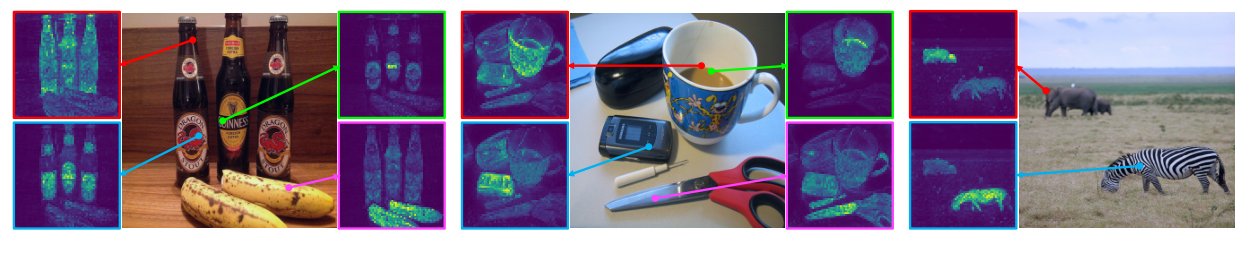
Figure 8: Self-attention for a set of reference points. We visualize the self-attention module from the last block of a ViT-S/8 trained with DINO. The network is able to separate objects, though it has been trained with no supervision at all.
图 8:一组参考点上的自注意力。 可视化用 DINO 训练的 ViT-S/8 最后一块的自注意力模块。尽管完全无监督训练,网络仍能分离物体。
B Methodology Comparison
B 方法比较
We compare the performance of different self-supervised frameworks, MoCo-v2 [15], SwAV [10] and BYOL [30] when using convnet or ViT. In Tab. 13, we see that when trained with ResNet-50 (convnet), DINO performs on par with SwAV and BYOL. However, DINO unravels its potential with ViT, outperforming MoCo-v2, SwAV and BYOL by large margins (+4.3% with linear and +6.2% with k-NN evaluations). In the rest of this section, we perform ablations to better understand the performance of DINO applied to ViT. In particular, we provide a detailed comparison with methods that either use a momentum encoder, namely MoCo-v2 and BYOL, and methods that use multi-crop, namely SwAV.
我们比较 MoCo-v2[15]、SwAV[10] 与 BYOL[30] 等不同自监督框架在卷积网络或 ViT 上的性能。表 13 显示:用 ResNet-50(卷积网络)训练时,DINO 与 SwAV、BYOL 持平;但 DINO 在 ViT 上潜力显现,大幅超过 MoCo-v2、SwAV 与 BYOL(线性 +4.3%,-NN +6.2%)。本节其余部分做消融以更好理解应用到 ViT 的 DINO 性能;特别与使用动量编码器的方法(MoCo-v2、BYOL)以及使用 multi-crop 的方法(SwAV)做详细比较。
| ResNet-50 | ViT-small | |||||
|---|---|---|---|---|---|---|
| Method | Linear | -NN | Linear | -NN | ||
| MoCo-v2 | 71.1 | 62.9 | 71.6 | 62.0 | ||
| BYOL | 72.7 | 65.4 | 71.4 | 66.6 | ||
| SwAV | 74.1 | 65.4 | 71.8 | 64.7 | ||
| DINO | 74.5 | 65.6 | 76.1 | 72.8 |
Table 13: Methodology comparison for DEIT-small and ResNet-50. We report ImageNet linear and -NN evaluations validation accuracy after 300 epochs pre-training. All numbers are run by us and match or outperform published results.
| ResNet-50 | ViT-small | |||||
|---|---|---|---|---|---|---|
| Method | Linear | -NN | Linear | -NN | ||
| MoCo-v2 | 71.1 | 62.9 | 71.6 | 62.0 | ||
| BYOL | 72.7 | 65.4 | 71.4 | 66.6 | ||
| SwAV | 74.1 | 65.4 | 71.8 | 64.7 | ||
| DINO | 74.5 | 65.6 | 76.1 | 72.8 |
表 13:DEIT-small 与 ResNet-50 的方法比较。 报告预训练 300 个 epoch 后 ImageNet 线性与 -NN 评估验证准确率。所有数字由我们运行,达到或超过已发表结果。
Relation to MoCo-v2 and BYOL.
In Tab. 14, we present the impact of ablating components that differ between DINO, MoCo-v2 and BYOL: the choice of loss, the predictor in the student head, the centering operation, the batch normalization in the projection heads, and finally, the multi-crop augmentation. The loss in DINO is a cross-entropy on sharpened softmax outputs (CE) while MoCo-v2 uses the InfoNCE contrastive loss (INCE) and BYOL a mean squared error on l2-normalized outputs (MSE). No sharpening is applied with the MSE criterion. Though, DINO surprisingly still works when changing the loss function to MSE, but this significantly alters the performance (see rows (1, 2) and (4, 9)). We also observe that adding a predictor has little impact (1, 3). However, in the case of BYOL, the predictor is critical to prevent collapse (7, 8) which is consistent with previous studies [16, 30]. Interestingly, we observe that the teacher output centering avoids collapse without predictor nor batch normalizations in BYOL (7, 9), though with a significant performance drop which can likely be explained by the fact that our centering operator is designed to work in combination with sharpening. Finally, we observe that multi-crop works particularly well with DINO and MoCo-v2, removing it hurts performance by (1 versus 4 and, 5 versus 6). Adding multi-crop to BYOL does not work out-of-the-box (7, 10) as detailed in Appendix E and further adaptation may be required.
与 MoCo-v2 和 BYOL 的关系。
表 14 展示消融 DINO、MoCo-v2 与 BYOL 之间差异组件的影响:损失选择、学生头中的预测器、中心化操作、投影头中的批归一化,以及 multi-crop 增强。DINO 的损失是对锐化 softmax 输出的交叉熵(CE),MoCo-v2 使用 InfoNCE 对比损失(INCE),BYOL 对 l2 归一化输出用均方误差(MSE)。MSE 准则下不做锐化。尽管如此,把损失函数换成 MSE 时 DINO 仍能工作,但性能显著下降(见第 1、2 行与第 4、9 行)。我们也观察到加预测器影响很小(1、3)。但在 BYOL 中预测器对防止崩塌至关重要(7、8),与先前研究一致[16, 30]。有趣的是,教师输出中心化使 BYOL 在无预测器也无批归一化时避免崩塌(7、9),但性能显著下降,很可能因为我们的中心化算子是为与锐化配合设计的。最后,multi-crop 对 DINO 与 MoCo-v2 特别有效,去掉会使性能下降 –(1 对 4,以及 5 对 6)。给 BYOL 加 multi-crop 不能开箱即用(7、10),细节见附录 E,可能需要进一步适配。
| Method | Loss | multi-crop | Center. | BN | Pred. | Top-1 | |
|---|---|---|---|---|---|---|---|
| 1 | DINO | CE | ✓ | ✓ | 76.1 | ||
| 2 | – | MSE | ✓ | ✓ | 62.4 | ||
| 3 | – | CE | ✓ | ✓ | ✓ | 75.6 | |
| 4 | – | CE | ✓ | 72.5 | |||
| 5 | MoCov2 | INCE | ✓ | 71.4 | |||
| 6 | INCE | ✓ | ✓ | 73.4 | |||
| 7 | BYOL | MSE | ✓ | ✓ | 71.4 | ||
| 8 | – | MSE | ✓ | 00.1 | |||
| 9 | – | MSE | ✓ | 52.6 | |||
| 10 | – | MSE | ✓ | ✓ | ✓ | 64.8 |
Table 14: Relation to MoCo-v2 and BYOL. We ablate the components that differ between DINO, MoCo-v2 and BYOL: the loss function (cross-entropy, CE, versus InfoNCE, INCE, versus mean-square error, MSE), the multi-crop training, the centering operator, the batch normalization in the projection heads and the student predictor. Models are run for 300 epochs with ViT-S/16. We report top-1 accuracy on ImageNet linear evaluation.
| Method | Loss | multi-crop | Center. | BN | Pred. | Top-1 | |
|---|---|---|---|---|---|---|---|
| 1 | DINO | CE | ✓ | ✓ | 76.1 | ||
| 2 | – | MSE | ✓ | ✓ | 62.4 | ||
| 3 | – | CE | ✓ | ✓ | ✓ | 75.6 | |
| 4 | – | CE | ✓ | 72.5 | |||
| 5 | MoCov2 | INCE | ✓ | 71.4 | |||
| 6 | INCE | ✓ | ✓ | 73.4 | |||
| 7 | BYOL | MSE | ✓ | ✓ | 71.4 | ||
| 8 | – | MSE | ✓ | 00.1 | |||
| 9 | – | MSE | ✓ | 52.6 | |||
| 10 | – | MSE | ✓ | ✓ | ✓ | 64.8 |
表 14:与 MoCo-v2 和 BYOL 的关系。 消融 DINO、MoCo-v2 与 BYOL 之间差异组件:损失函数(交叉熵 CE、InfoNCE INCE、均方误差 MSE)、multi-crop 训练、中心化算子、投影头中的批归一化以及学生预测器。模型用 ViT-S/16 运行 300 个 epoch。报告 ImageNet 线性评估 top-1。
| Method | Momentum | Operation | Top-1 | |
|---|---|---|---|---|
| 1 | DINO | ✓ | Centering | 76.1 |
| 2 | – | ✓ | Softmax(batch) | 75.8 |
| 3 | – | ✓ | Sinkhorn-Knopp | 76.0 |
| 4 | – | Centering | 00.1 | |
| 5 | – | Softmax(batch) | 72.2 | |
| 6 | SwAV | Sinkhorn-Knopp | 71.8 |
Table 15: Relation to SwAV. We vary the operation on the teacher output between centering, a softmax applied over the batch dimension and the Sinkhorn-Knopp algorithm. We also ablate the Momentum encoder by replacing it with a hard copy of the student with a stop-gradient as in SwAV. Models are run for 300 epochs with ViT-S/16. We report top-1 accuracy on ImageNet linear evaluation.
| Method | Momentum | Operation | Top-1 | |
|---|---|---|---|---|
| 1 | DINO | ✓ | Centering | 76.1 |
| 2 | – | ✓ | Softmax(batch) | 75.8 |
| 3 | – | ✓ | Sinkhorn-Knopp | 76.0 |
| 4 | – | Centering | 00.1 | |
| 5 | – | Softmax(batch) | 72.2 | |
| 6 | SwAV | Sinkhorn-Knopp | 71.8 |
表 15:与 SwAV 的关系。 在中心化、沿 batch 维的 softmax 与 Sinkhorn-Knopp 算法之间变换教师输出上的操作。也通过用带 stop-gradient 的学生硬拷贝替换动量编码器来消融动量,如 SwAV。模型用 ViT-S/16 运行 300 个 epoch。报告 ImageNet 线性评估 top-1。
Relation to SwAV.
In Tab. 15, we evaluate the differences between DINO and SwAV: the presence of the momentum encoder and the operation on top of the teacher output. In absence of the momentum, a copy of the student with a stop-gradient is used. We consider three operations on the teacher output: Centering, Sinkhorn-Knopp or a Softmax along the batch axis. The Softmax is similar to a single Sinkhorn-Knopp iteration as detailed in the next paragraph. First, these ablations show that using a momentum encoder significantly improves the performance for ViT (3 versus 6, and 2 versus 5). Second, the momentum encoder also avoids collapse when using only centering (row 1). In the absence of momentum, centering the outputs does not work (4) and more advanced operations are required (5, 6). Overall, these ablations highlight the importance of the momentum encoder, not only for performance but also to stabilize training, removing the need for normalization beyond centering.
与 SwAV 的关系。
表 15 评估 DINO 与 SwAV 的差异:是否有动量编码器,以及教师输出上的操作。无动量时使用带 stop-gradient 的学生副本。教师输出上考虑三种操作:中心化、Sinkhorn-Knopp 或沿 batch 轴的 Softmax。Softmax 类似单次 Sinkhorn-Knopp 迭代,详见下一段。首先,这些消融表明对 ViT 使用动量编码器显著提升性能(3 对 6,以及 2 对 5)。其次,动量编码器也使仅用中心化即可避免崩塌(第 1 行)。无动量时,对输出做中心化无效(4),需要更高级操作(5、6)。总体而言,这些消融突出了动量编码器的重要性——不仅为了性能,也为了稳定训练,使归一化只需中心化即可。
Details on the Softmax(batch) variant.
The iterative Sinkhorn-Knopp algorithm [17] used in SwAV [10] is implemented simply with the following PyTorch style code.
Softmax(batch) 变体细节。
SwAV[10] 中使用的迭代 Sinkhorn-Knopp 算法[17]可用如下 PyTorch 风格代码简单实现。
When performing a single Sinkhorn iteration (num_iters=1) the implementation can be highly simplified into only two lines of code, which is our softmax(batch) variant:
当只做一次 Sinkhorn 迭代(num_iters=1)时,实现可高度简化为两行代码,也就是我们的 softmax(batch) 变体:
We have seen in Tab. 15 that this highly simplified variant of SwAV works competitively with SwAV. Intuitively, the softmax operation on the batch axis allows to select for each dimension (or “cluster”) its best matches in the batch.
表 15 显示这一高度简化的 SwAV 变体与 SwAV 竞争力相当。直觉上,沿 batch 轴的 softmax 使每个维(或“簇”)能在批次中选出最佳匹配。
Validating our implementation.
We observe in Tab. 13 that our reproduction of BYOL, MoCo-v2, SwAV matches or outperforms the corresponding published numbers with ResNet-50. Indeed, we obtain for BYOL while [30] report in this -epochs setting. We obtain for MoCo after epochs of training while [15] report after epochs of training. Our improvement compared to the implementation of [15] can be explained by the use of a larger projection head (3-layer, use of batch-normalizations and projection dimension of ).
验证我们的实现。
表 13 显示我们对 BYOL、MoCo-v2、SwAV 的复现达到或超过 ResNet-50 上已发表数字。例如 BYOL 我们得到 ,而[30]在该 -epoch 设定报告 ;MoCo 训练 个 epoch 得到 ,而[15]在 个 epoch 后报告 。相对[15]实现的改进可解释为使用了更大的投影头(3 层、使用批归一化、投影维为 )。
Relation to other works.
DINO is also related to UIC [14] that use outputs from the previous epoch as hard pseudo-labels for “unsupervised classification”. However, we use centering to prevent collapse while UIC resorts to balance sampling techniques as in [8]. Our work can be interpreted as a soft UIC variant with momentum teacher.
与其他工作的关系。
DINO 也与 UIC[14] 相关,后者用上一 epoch 的输出作为“无监督分类”的硬伪标签。但我们用中心化防止崩塌,而 UIC 诉诸如[8]中的平衡采样技术。本工作可理解为带动量教师的软 UIC 变体。
The concurrent work CsMI [77] also exhibits strong performance with simple k-NN classifiers on ImageNet, even with convnets. As DINO, CsMI combines a momentum network and multi-crop training, which we have seen are both crucial for good k-NN performance in our experiments with ViTs. We believe studying this work would help us identifying more precisely the components important for good -NN performance and leave this investigation for future work.
并行工作 CsMI[77] 在 ImageNet 上用简单 -NN 分类器也表现出强性能,即便用卷积网络。与 DINO 一样,CsMI 结合动量网络与 multi-crop 训练,而我们在 ViT 实验中看到这两者对良好 -NN 性能都至关重要。我们认为研究该工作有助于更精确识别对良好 -NN 性能重要的组件,并将此调查留给未来工作。
C Projection Head
C 投影头
Similarly to other self-supervised frameworks, using a projection head [12] improves greatly the accuracy of our method. The projection head starts with a -layer multi-layer perceptron (MLP). The hidden layers are 2048d and are with gaussian error linear units (GELU) activations. The last layer of the MLP is without GELU. Then we apply a normalization and a weight normalized fully connected layer [16, 61] with dimensions. This design is inspired from the projection head with a “prototype layer” used in SwAV [10]. We do not apply batch normalizations.
与其他自监督框架类似,使用投影头[12]显著提升本方法准确率。投影头以 层多层感知机(MLP)开始。隐层为 2048 维,带高斯误差线性单元(GELU)激活;MLP 最后一层不加 GELU。然后施加 归一化与权值归一化的全连接层[16, 61],输出 维。该设计受 SwAV[10] 中带“原型层”的投影头启发。我们不加批归一化。
BN-free system.
Unlike standard convnets, ViT architectures do not use batch normalizations (BN) by default.
无 BN 系统。
与标准卷积网络不同,ViT 架构默认不使用批归一化(BN)。
| ViT-S, 100 epochs | heads w/o BN | heads w/ BN |
|---|---|---|
| -NN top-1 | 69.7 | 68.6 |
| ViT-S, 100 epochs | heads w/o BN | heads w/ BN |
|---|---|---|
| -NN top-1 | 69.7 | 68.6 |
表:ViT-S 训练 100 个 epoch 时,投影头有/无 BN 的 -NN top-1。
Therefore, when applying DINO to ViT we do not use any BN also in the projection heads. In this table we evaluate the impact of adding BN in the heads. We observe that adding BN in the projection heads has little impact, showing that BN is not important in our framework. Overall, when applying DINO to ViT, we do not use any BN anywhere, making the system entirely BN-free. This is a great advantage of DINO + ViT to work at state-of-the-art performance without requiring any BN. Indeed, training with BN typically slows down trainings considerably, especially when these BN modules need to be synchronized across processes [33, 10, 9, 30].
因此把 DINO 用到 ViT 时,投影头也不加任何 BN。本表评估在头中加入 BN 的影响。可见加入 BN 影响很小,说明 BN 在本框架中不重要。*总体而言,把 DINO 用到 ViT 时,我们在任何地方都不使用 BN,使系统完全无 BN。*这对 DINO + ViT 在达到当时最优性能的同时不需要任何 BN 是一大优势。因为带 BN 的训练通常会显著变慢,尤其是这些 BN 模块需要跨进程同步时[33, 10, 9, 30]。
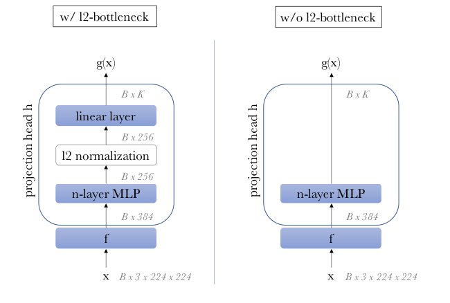
Figure 9: Projection head design w/ or w/o l2-norm bottleneck.
图 9:有/无 l2 归一化瓶颈的投影头设计。
L2-normalization bottleneck in projection head.
We illustrate the design of the projection head with or without l2-normalization bottleneck in Fig. 9.
投影头中的 L2 归一化瓶颈。
我们在图 9 中展示有/无 l2 归一化瓶颈的投影头设计。
| # proj. head linear layers | ||||
|---|---|---|---|---|
| w/ l2-norm bottleneck | – | 62.2 | 68.0 | 69.3 |
| w/o l2-norm bottleneck | 61.6 | 62.9 | 0.1 | 0.1 |
| # proj. head linear layers | ||||
|---|---|---|---|---|
| w/ l2-norm bottleneck | – | 62.2 | 68.0 | 69.3 |
| w/o l2-norm bottleneck | 61.6 | 62.9 | 0.1 | 0.1 |
表:有/无 l2 归一化瓶颈时,投影头线性层数对 -NN top-1 的影响。
We evaluate the accuracy of DINO models trained with or without l2-normalization bottleneck and we vary the number of linear layers in the projection head. With l2 bottleneck, the total number of linear layers is ( from the MLP and from the weight normalized layer) while without bottleneck the total number of linear layers is in the head. In this table, we report ImageNet top-1 -NN evaluation accuracy after 100 epochs pre-training with ViT-S/16. The output dimensionality is set to in this experiment. We observe that DINO training fails without the l2-normalization bottleneck when increasing the depth of the projection head. L2-normalization bottleneck stabilizes the training of DINO with deep projection head. We observe that increasing the depth of the projection head improves accuracy. Our default is to use a total of 4 linear layers: 3 are in the MLP and one is after the l2 bottleneck.
我们评估有/无 l2 归一化瓶颈训练的 DINO 模型准确率,并改变投影头中线性层数量。有 l2 瓶颈时,线性层总数为 (MLP 中 层加权值归一化层 1 层);无瓶颈时头中线性层总数为 。本表报告用 ViT-S/16 预训练 100 个 epoch 后的 ImageNet top-1 -NN 评估准确率。本实验输出维 设为 。可见加深投影头且无 l2 归一化瓶颈时 DINO 训练会失败。L2 归一化瓶颈稳定了带深投影头的 DINO 训练。加深投影头可提升准确率。我们默认使用共 4 个线性层:3 个在 MLP 中,1 个在 l2 瓶颈之后。
Output dimension.
In this table, we evaluate the effect of varying the output dimensionality .
输出维。
本表评估改变输出维 的影响。
| 1024 | 4096 | 16384 | 65536 | 262144 | |
|---|---|---|---|---|---|
| -NN top-1 | 67.8 | 69.3 | 69.2 | 69.7 | 69.1 |
| 1024 | 4096 | 16384 | 65536 | 262144 | |
|---|---|---|---|---|---|
| -NN top-1 | 67.8 | 69.3 | 69.2 | 69.7 | 69.1 |
表:不同输出维 下的 -NN top-1。
We observe that a large output dimensionality improves the performance. We note that the use of l2-normalization bottleneck permits to use a large output dimension with a moderate increase in the total number of parameters. Our default is to use equals to 65536 and for the bottleneck.
可见较大的输出维可提升性能。我们注意到使用 l2 归一化瓶颈使得在总参数量适度增加的情况下仍可使用大输出维。默认取 为 65536,瓶颈维 。
GELU activations.
By default, the activations used in ViT are gaussian error linear units (GELU).
GELU 激活。
默认情况下,ViT 使用的激活是高斯误差线性单元(GELU)。
| ViT-S, 100 epochs | heads w/ GELU | heads w/ ReLU |
|---|---|---|
| -NN top-1 | 69.7 | 68.9 |
| ViT-S, 100 epochs | heads w/ GELU | heads w/ ReLU |
|---|---|---|
| -NN top-1 | 69.7 | 68.9 |
表:投影头使用 GELU 或 ReLU 的 -NN top-1(ViT-S,100 个 epoch)。
Therefore, for consistency within the architecture, we choose to use GELU also in the projection head. We evaluate the effect of using ReLU instead of GELU in this table and observe that changing the activation unit to ReLU has relatively little impact.
因此为了架构内一致性,我们选择在投影头中也使用 GELU。本表评估用 ReLU 替代 GELU 的影响,可见改用 ReLU 影响相对较小。
D Additional Ablations
D 补充消融
We have detailed in the main paper that the combination of centering and sharpening is important to avoid collapse in DINO. We ablate the hyperparameters for these two operations in the following. We also study the impact of training length and some design choices for the ViT networks.
正文已详述中心化与锐化的组合对避免 DINO 崩塌很重要。下面消融这两种操作的超参。我们也研究训练长度以及 ViT 网络若干设计选择的影响。
Online centering.
We study the impact of the smoothing parameters in the update rule for the center used in the output of the teacher network.
在线中心化。
我们研究教师网络输出所用中心 的更新规则中平滑参数的影响。
| 0 | 0.9 | 0.99 | 0.999 | |
|---|---|---|---|---|
| -NN top-1 | 69.1 | 69.7 | 69.4 | 0.1 |
| 0 | 0.9 | 0.99 | 0.999 | |
|---|---|---|---|---|
| -NN top-1 | 69.1 | 69.7 | 69.4 | 0.1 |
表:中心化平滑参数 对 -NN top-1 的影响。
The convergence is robust to a wide range of smoothing, and the model only collapses when the update is too slow, i.e., .
收敛对宽范围的平滑都稳健,仅当更新过慢(即 )时模型才崩塌。
Sharpening.
We enforce sharp targets by tuning the teacher softmax temperature parameter . In this table, we observe that a temperature lower than is required to avoid collapse.
锐化。
我们通过调节教师 softmax 温度参数 强制得到锐利目标。本表显示需要低于 的温度才能避免崩塌。
| -NN top-1 | 43.9 | 66.7 | 69.6 | 68.7 | 0.1 | 69.7 |
| -NN top-1 | 43.9 | 66.7 | 69.6 | 68.7 | 0.1 | 69.7 |
表:教师温度 对 -NN top-1 的影响。
When the temperature is higher than , the training loss consistently converges to . However, we have observed that using higher temperature than does not collapse if we start the training from a smaller value and increase it during the first epochs. In practice, we use a linear warm-up for from to during the first epochs of training. Finally, note that (extreme sharpening) correspond to the argmax operation and leads to one-hot hard distributions.
当温度高于 时,训练损失一贯收敛到 。不过我们观察到:若从较小值开始并在前几个 epoch 升高,高于 的温度也不会崩塌。实践中,我们对 在训练前 个 epoch 从 线性升温到 。最后注意 (极端锐化)对应 argmax 操作,并导致 one-hot 硬分布。
Longer training.
We observe in this table that longer training improves the performance of DINO applied to ViT-Small.
更长训练。
本表显示更长训练可提升应用到 ViT-Small 的 DINO 性能。
| DINO ViT-S | 100-ep | 300-ep | 800-ep |
|---|---|---|---|
| -NN top-1 | 70.9 | 72.8 | 74.5 |
| DINO ViT-S | 100-ep | 300-ep | 800-ep |
|---|---|---|---|
| -NN top-1 | 70.9 | 72.8 | 74.5 |
表:不同训练长度下 DINO ViT-S 的 -NN top-1。
This observation is consistent with self-supervised results obtained with convolutional architectures [12]. We note that in our experiments with BYOL on ViT-S, training longer than epochs has been leading to worse performance compare our epochs run. For this reason we report BYOL for 300 epochs in Tab. 2 while SwAV, MoCo-v2 and DINO are trained for 800 epochs.
这一观察与卷积架构上的自监督结果一致[12]。我们注意到在 ViT-S 上的 BYOL 实验中,训练超过 个 epoch 会导致比我们的 epoch 运行更差的性能。因此表 2 中 BYOL 报告 300 个 epoch,而 SwAV、MoCo-v2 与 DINO 训练 800 个 epoch。
The teacher outperforms the student.
We have shown in Fig. 6 that the momentum teacher outperforms the student with ViT and we show in this Figure that it is also the case with ResNet-50.
教师优于学生。
图 6 已显示动量教师在 ViT 上优于学生;本图表明用 ResNet-50 时同样如此。
The fact that the teacher continually outperforms the student further encourages the interpretation of DINO as a form of Mean Teacher [65] self-distillation. Indeed, as motivated in Tarvainen et al. [65], weight averaging usually produces a better model than the individual models from each iteration [51]. By aiming a target obtained with a teacher better than the student, the student’s representations improve. Consequently, the teacher also improves since it is built directly from the student weights.
教师持续优于学生这一事实进一步鼓励把 DINO 解释为一种 Mean Teacher[65] 自蒸馏。的确,如 Tarvainen 等[65]所论证,权重平均通常产生比各迭代单独模型更好的模型[51]。通过瞄准由优于学生的教师得到的目标,学生的表征得到改善;因而教师也改善,因为它直接由学生权重构建。
Self-attention maps from supervised versus self-supervised learning.
We evaluate the masks obtained by thresholding the self-attention maps to keep 80% of the mass.
有监督与自监督学习的自注意力图。
我们评估通过对自注意力图阈值、保留 80% 质量得到的掩码。
| ViT-S/16 weights | |
|---|---|
| Random weights | 22.0 |
| Supervised | 27.3 |
| DINO | 45.9 |
| DINO w/o multicrop | 45.1 |
| MoCo-v2 | 46.3 |
| BYOL | 47.8 |
| SwAV | 46.8 |
| ViT-S/16 weights | |
|---|---|
| Random weights | 22.0 |
| Supervised | 27.3 |
| DINO | 45.9 |
| DINO w/o multicrop | 45.1 |
| MoCo-v2 | 46.3 |
| BYOL | 47.8 |
| SwAV | 46.8 |
表:不同 ViT-S/16 权重下阈值自注意力掩码与 VOC 真值的 Jaccard 相似度。
We compare the Jaccard similarity between the ground truth and these masks on the validation images of PASCAL VOC12 dataset for different ViT-S trained with different frameworks. The properties that self-attention maps from ViT explicitly contain the scene layout and, in particular, object boundaries is observed across different self-supervised methods.
我们在 PASCAL VOC12 验证集图像上,比较用不同框架训练的不同 ViT-S 所得掩码与真值之间的 Jaccard 相似度。ViT 自注意力图显式包含场景布局、尤其是物体边界这一性质,在不同自监督方法中均可观察到。
Impact of the number of heads in ViT-S.
We study the impact of the number of heads in ViT-S on the accuracy and throughput (images processed per second at inference time on a singe V100 GPU).
ViT-S 中头数的影响。
我们研究 ViT-S 中头数对准确率与吞吐(单张 V100 GPU 推理时每秒处理图像数)的影响。
| # heads | dim | dim/head | # params | im/sec | -NN |
|---|---|---|---|---|---|
| 6 | 384 | 64 | 21 | 1007 | 72.8 |
| 8 | 384 | 48 | 21 | 971 | 73.1 |
| 12 | 384 | 32 | 21 | 927 | 73.7 |
| 16 | 384 | 24 | 21 | 860 | 73.8 |
| # heads | dim | dim/head | # params | im/sec | -NN |
|---|---|---|---|---|---|
| 6 | 384 | 64 | 21 | 1007 | 72.8 |
| 8 | 384 | 48 | 21 | 971 | 73.1 |
| 12 | 384 | 32 | 21 | 927 | 73.7 |
| 16 | 384 | 24 | 21 | 860 | 73.8 |
表:ViT-S 不同头数下的参数量、吞吐与 -NN。
We find that increasing the number of heads improves the performance, at the cost of a slighlty worse throughput. In our paper, all experiments are run with the default model DeiT-S [69], i.e. with heads only.
我们发现增加头数可提升性能,代价是吞吐略降。本文所有实验均使用默认模型 DeiT-S[69],即仅 个头。
E Multi-crop
In this Appendix, we study a core component of DINO: multi-crop training [10].
本附录研究 DINO 的核心组件:multi-crop 训练[10]。
Range of scales in multi-crop.
For generating the different views, we use the RandomResizedCrop method from torchvision.transforms module in PyTorch.
Multi-crop 中的尺度范围。
生成不同视图时,我们使用 PyTorch 中 torchvision.transforms 模块的 RandomResizedCrop 方法。
| (0.05, ), (, 1), : | 0.08 | 0.16 | 0.24 | 0.32 | 0.48 |
|---|---|---|---|---|---|
| -NN top-1 | 65.6 | 68.0 | 69.7 | 69.8 | 69.5 |
| (0.05, ), (, 1), : | 0.08 | 0.16 | 0.24 | 0.32 | 0.48 |
|---|---|---|---|---|---|
| -NN top-1 | 65.6 | 68.0 | 69.7 | 69.8 | 69.5 |
表:multi-crop 尺度参数 对 -NN top-1 的影响。
We sample two global views with scale range before resizing them to and local views with scale sampled in the range resized to pixels. Note that we arbitrarily choose to have non-overlapping scaling range for the global and local views following the original design of SwAV. However, the ranges could definitely be overlapping and experimenting with finer hyperparameters search could lead to a more optimal setting. In this table, we vary the parameter that controls the range of scales used in multi-crop and find the optimum to be around in our experiments. We note that this is higher than the parameter used in SwAV which is of .
我们采样两个尺度范围在 、再缩放到 的全局视图,以及 6 个尺度在 内采样、缩放到 像素的局部视图。注意我们任意选择让全局与局部视图的缩放范围不重叠,以遵循 SwAV 的原始设计。不过范围完全可以重叠,更细致的超参搜索可能导致更优设定。本表改变控制 multi-crop 尺度范围的参数 ,发现在我们实验中最优约在 。注意这高于 SwAV 使用的 。
Multi-crop in different self-supervised frameworks.
We compare different recent self-supervised learning frameworks, namely MoCo-v2 [15], BYOL [30] and SwAV [10] with ViT-S/16 architecture.
不同自监督框架中的 Multi-crop。
我们用 ViT-S/16 架构比较近期自监督学习框架 MoCo-v2[15]、BYOL[30] 与 SwAV[10]。
| crops | |||||
|---|---|---|---|---|---|
| eval | -NN | linear | -NN | linear | |
| BYOL | 66.6 | 71.4 | 59.8 | 64.8 | |
| SwAV | 60.5 | 68.5 | 64.7 | 71.8 | |
| MoCo-v2 | 62.0 | 71.6 | 65.4 | 73.4 | |
| DINO | 67.9 | 72.5 | 72.7 | 75.9 |
| crops | |||||
|---|---|---|---|---|---|
| eval | -NN | linear | -NN | linear | |
| BYOL | 66.6 | 71.4 | 59.8 | 64.8 | |
| SwAV | 60.5 | 68.5 | 64.7 | 71.8 | |
| MoCo-v2 | 62.0 | 71.6 | 65.4 | 73.4 | |
| DINO | 67.9 | 72.5 | 72.7 | 75.9 |
表:有/无 multi-crop 时各框架的 -NN 与线性评估。
For fair comparisons, all models are pretrained either with two crops or with multi-crop [10] training, i.e. two crops and six crops for each image. We report -NN and linear probing evaluations after 300 epochs of training. Multi-crop does not benefit all frameworks equally, which has been ignored in benchmarks considering only the two crops setting [16]. The effectiveness of multi-crop depends on the considered framework, which positions multi-crop as a core component of a model and not a simple “add-ons” that will boost any framework the same way. Without multi-crop, DINO has better accuracy than other frameworks, though by a moderate margin (1%). Remarkably, DINO benefits the most from multi-crop training ( in linear eval). Interestingly, we also observe that the ranking of the frameworks depends on the evaluation protocol considered.
为公平比较,所有模型要么用两个 裁剪预训练,要么用 multi-crop[10] 训练,即每张图两个 裁剪加六个 裁剪。报告训练 300 个 epoch 后的 -NN 与线性探测评估。Multi-crop 并非同等惠及所有框架——仅考虑双裁剪设定的基准[16]忽略了这一点。Multi-crop 的有效性取决于所考虑的框架,从而把它定位为模型的核心组件,而非以相同方式提升任何框架的简单“附加件”。无 multi-crop 时,DINO 准确率仍高于其他框架,但优势适中(1%)。显著的是,DINO 从 multi-crop 训练中获益最大(线性评估 +)。有趣的是,我们也观察到框架排名取决于所考虑的评估协议。
Training BYOL with multi-crop.
When applying multi-crop to BYOL with ViT-S, we observe the transfer performance is higher than the baseline without multi-crop for the first training epochs.
用 multi-crop 训练 BYOL。
把 multi-crop 用到 ViT-S 上的 BYOL 时,我们观察到前几个训练 epoch 的迁移性能高于无 multi-crop 的基线。
However, the transfer performance growth rate is slowing down and declines after a certain amount of training. We have performed learning rate, weight decay, multi-crop parameters sweeps for this setting and systematically observe the same pattern. More precisely, we experiment with {, , , , , } for learning rate base values, with {, , } for weight decay and with different number of small crops: {2, 4, 6}. All our runs are performed with synchronized batch normalizations in the heads. When using a low learning rate, we did not observe the performance break point, i.e. the transfer performance was improving continually during training, but the overall accuracy was low. We have tried a run with multi-crop training on ResNet-50 where we also observe the same behavior. Since integrating multi-crop training to BYOL is not the focus of this study we did not push that direction further. However, we believe this is worth investigating why multi-crop does not combine well with BYOL in our experiments and leave this for future work.
然而迁移性能的增长率在减缓,并在一定训练量后下降。我们对该设定做了学习率、权重衰减、multi-crop 参数扫描,系统观察到同一模式。更具体地,学习率基值试验 {, , , , , },权重衰减试验 {, , },小裁剪数量试验 {2, 4, 6}。所有运行在头中使用同步批归一化。使用低学习率时,我们未观察到性能断点,即迁移性能在训练中持续提升,但总体准确率偏低。我们也在 ResNet-50 上试过 multi-crop 训练,观察到同样行为。由于把 multi-crop 训练整合进 BYOL 并非本研究重点,我们未继续推进该方向。不过我们认为值得探究为何在我们的实验中 multi-crop 与 BYOL 配合不佳,并留给未来工作。
F Evaluation Protocols
F 评估协议
F.1 -NN classification
Following the setting of Wu et al. [73], we evaluate the quality of features with a simple weighted Nearest Neighbor classifier. We freeze the pretrained model to compute and store the features of the training data of the downstream task. To classify a test image , we compute its representation and compare it against all stored training features . The representation of an image is given by the output [CLS] token: it has dimensionality for ViT-S and for ViT-B. The top NN (denoted ) are used to make a prediction via weighted voting. Specifically, the class gets a total weight of , where is a contribution weight. We use with equals to as in [73] which we do not tune. We evaluate different values for and find that is consistently leading to the best accuracy across our runs. This evaluation protocol does not require hyperparameter tuning, nor data augmentation and can be run with only one pass over the downstream dataset.
F.1 -NN 分类
遵循 Wu 等[73]的设定,我们用简单的加权 最近邻分类器评估特征质量。冻结预训练模型,计算并存储下游任务训练数据的特征。要对测试图像 分类,计算其表征并与所有存储的训练特征 比较。图像表征由输出 [CLS] token 给出:ViT-S 维数为 ,ViT-B 为 。用前 个 NN(记为 )经加权投票做预测。具体地,类别 的总权重为 ,其中 为贡献权重。我们使用 , 取 如[73],且不调参。我们评估不同 值,发现跨运行 一贯给出最佳准确率。该评估协议无需超参调优或数据增强,只需对下游数据集扫一遍即可运行。
F.2 Linear classification
Following common practice in self-supervised learning, we evaluate the representation quality with a linear classifier. The projection head is removed, and we train a supervised linear classifier on top of frozen features. This linear classifier is trained with SGD and a batch size of during epochs on ImageNet. We do not apply weight decay. For each model, we sweep the learning rate value. During training, we apply only random resizes crops (with default parameters from PyTorch RandomResizedCrop) and horizontal flips as data augmentation. We report central-crop top-1 accuracy. When evaluating convnets, the common practice is to perform global average pooling on the final feature map before the linear classifier. In the following, we describe how we adapt this design when evaluating ViTs.
F.2 线性分类
遵循自监督学习常见做法,我们用线性分类器评估表征质量。去掉投影头,在冻结特征上训练有监督线性分类器。该线性分类器用 SGD、批次大小 在 ImageNet 上训练 个 epoch。不加权重衰减。对每个模型扫描学习率。训练时数据增强仅用随机缩放裁剪(PyTorch RandomResizedCrop 默认参数)与水平翻转。报告中心裁剪 top-1 准确率。评估卷积网络时,常见做法是在最终特征图上做全局平均池化再接线性分类器。下面说明评估 ViT 时如何适配该设计。
ViT-S representations for linear eval.
Following the feature-based evaluations in BERT [18], we concatenate the [CLS] tokens from the last layers.
线性评估用的 ViT-S 表征。
遵循 BERT[18] 中的基于特征评估,我们拼接最后 层的 [CLS] token。
| concatenate last layers | ||||
|---|---|---|---|---|
| representation dim | 384 | 768 | 1536 | 2304 |
| ViT-S/16 linear eval | 76.1 | 76.6 | 77.0 | 77.0 |
| concatenate last layers | ||||
|---|---|---|---|---|
| representation dim | 384 | 768 | 1536 | 2304 |
| ViT-S/16 linear eval | 76.1 | 76.6 | 77.0 | 77.0 |
表:拼接不同层数 的 [CLS] 对 ViT-S/16 线性评估的影响。
We experiment with the concatenation of a different number of layers and similarly to [18] we find to be optimal.
我们试验拼接不同层数 ,并与[18]类似地发现 最优。
ViT-B representations for linear eval.
With ViT-B we did not find that concatenating the representations from the last layers to provide any performance gain, and consider the final layer only ().
线性评估用的 ViT-B 表征。
对 ViT-B,我们未发现拼接最后 层表征能带来任何性能增益,因而只考虑最后一层()。
| pooling strategy | [CLS] tok. | concatenate [CLS] tok. |
|---|---|---|
| only | and avgpooled patch tok. | |
| representation dim | 768 | 1536 |
| ViT-B/16 linear eval | 78.0 | 78.2 |
| pooling strategy | [CLS] tok. | concatenate [CLS] tok. |
|---|---|---|
| only | and avgpooled patch tok. | |
| representation dim | 768 | 1536 |
| ViT-B/16 linear eval | 78.0 | 78.2 |
表:ViT-B/16 线性评估的池化策略比较。
In this setting, we adapt the pipeline used in convnets with global average pooling on the output patch tokens. We concatenate these pooled features to the final [CLS] output token.
在该设定下,我们适配卷积网络中在输出 patch token 上做全局平均池化的流程,把这些池化特征拼接到最终 [CLS] 输出 token。
G Self-Attention Visualizations
G 自注意力可视化
We provide more self-attention visualizations in Fig. 8 and in Fig. 10. The images are randomly selected from COCO validation set, and are not used during training of DINO. In Fig. 8, we show the self-attention from the last layer of a DINO ViT-S/8 for several reference points.
我们在图 8 与图 10 中提供更多自注意力可视化。图像从 COCO 验证集随机选取,未用于 DINO 训练。图 8 展示 DINO ViT-S/8 最后一层对若干参考点的自注意力。
H Class Representation
H 类别表征
As a final visualization, we propose to look at the distribution of ImageNet concepts in the feature space from DINO. We represent each ImageNet class with the average feature vector for its validation images. We reduce the dimension of these features to 30 with PCA, and run t-SNE with a perplexity of 20, a learning rate of 200 for 5000 iterations. We present the resulting class embeddings in Fig. 11. Our model recovers structures between classes: similar animal species are grouped together, forming coherent clusters of birds (top) or dogs, and especially terriers (far right).
作为最终可视化,我们查看 DINO 特征空间中 ImageNet 概念的分布。用验证集图像的平均特征向量表示每个 ImageNet 类。用 PCA 把这些特征降到 30 维,再以困惑度 20、学习率 200 运行 t-SNE 共 5000 次迭代。结果类别嵌入见图 11。我们的模型恢复了类间结构:相近动物物种聚在一起,形成连贯的鸟类簇(上方)或狗类簇,尤其是㹴犬(最右侧)。
| DINO | Supervised | DINO | Supervised | ||||||||||||||||||||
|---|---|---|---|---|---|---|---|---|---|---|---|---|---|---|---|---|---|---|---|---|---|---|---|
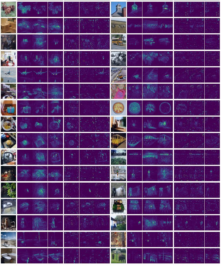
Figure 10: Self-attention heads from the last layer. We look at the attention map when using the [CLS] token as a query for the different heads in the last layer. Note that the [CLS] token is not attached to any label or supervision.
| DINO | Supervised | DINO | Supervised | ||||||||||||||||||||
|---|---|---|---|---|---|---|---|---|---|---|---|---|---|---|---|---|---|---|---|---|---|---|---|
图 10:最后一层的自注意力头。 我们查看以 [CLS] token 为查询时最后一层不同头的注意力图。注意 [CLS] token 未附着任何标签或监督。
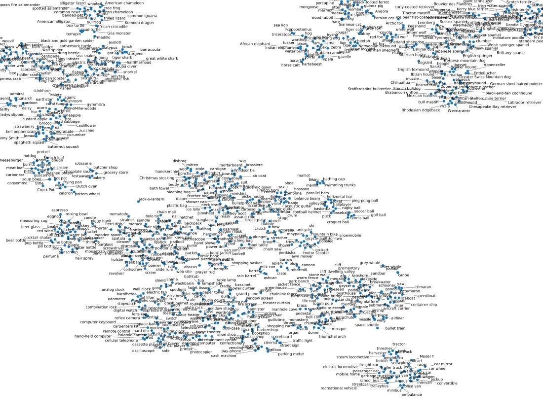
Figure 11: t-SNE visualization of ImageNet classes as represented using DINO. For each class, we obtain the embedding by taking the average feature for all images of that class in the validation set.
图 11:用 DINO 表示的 ImageNet 类别的 t-SNE 可视化。对每个类,取其验证集全部图像的平均特征作为嵌入。