Directional Message Passing for Molecular Graphs

分子图上的有向消息传递

Johannes Gasteiger    Janek Groß & Stephan Günnemann Affiliation:  Technical University of Munich, Germany Email:  {j.gasteiger,grossja,guennemann}@in.tum.de

Abstract

摘要

Graph neural networks have recently achieved great successes in predicting quantum mechanical properties of molecules. These models represent a molecule as a graph using only the distance between atoms (nodes). They do not, however, consider the spatial direction from one atom to another, despite directional information playing a central role in empirical potentials for molecules, e.g. in angular potentials. To alleviate this limitation we propose directional message passing, in which we embed the messages passed between atoms instead of the atoms themselves. Each message is associated with a direction in coordinate space. These directional message embeddings are rotationally equivariant since the associated directions rotate with the molecule. We propose a message passing scheme analogous to belief propagation, which uses the directional information by transforming messages based on the angle between them. Additionally, we use spherical Bessel functions and spherical harmonics to construct theoretically well-founded, orthogonal representations that achieve better performance than the currently prevalent Gaussian radial basis representations while using fewer than $\nicefrac{{1}}{{4}}$ of the parameters. We leverage these innovations to construct the directional message passing neural network (DimeNet). DimeNet outperforms previous GNNs on average by $76\text{\,}\mathrm{\%}$ on MD17 and by $31\text{\,}\mathrm{\%}$ on QM9. Our implementation is available online. [^1]

图神经网络近来在预测分子量子力学性质上取得很大成功。这些模型把分子表示为图，通常只使用原子（节点）之间的距离。然而它们并不考虑从一个原子到另一个原子的空间方向，尽管方向信息在分子经验势中扮演核心角色，例如角势。为缓解这一限制，我们提出有向消息传递：嵌入在原子之间传递的消息，而非原子本身。每条消息与坐标空间中的一个方向相关联。由于关联方向随分子旋转，这些有向消息嵌入是旋转等变的。我们提出一种类似信念传播的消息传递方案，依据消息之间的夹角变换消息，从而利用方向信息。此外，我们用球贝塞尔函数与球谐函数构造理论上有根基、正交的表示，在参数少于当前流行高斯径向基表示的 $\nicefrac{{1}}{{4}}$ 时仍取得更好表现。我们把这些创新整合为有向消息传递神经网络（DimeNet）。DimeNet 在 MD17 上平均优于先前 GNN $76\text{\,}\mathrm{\%}$，在 QM9 上平均优于 $31\text{\,}\mathrm{\%}$。实现已开源。[^1]

1 Introduction

1 引言

In recent years scientists have started leveraging machine learning to reduce the computation time required for predicting molecular properties from a matter of hours and days to mere milliseconds. With the advent of graph neural networks (GNNs) this approach has recently experienced a small revolution, since they do not require any form of manual feature engineering and significantly outperform previous models (Gilmer et al., 2017; Schütt et al., 2017). GNNs model the complex interactions between atoms by embedding each atom in a high-dimensional space and updating these embeddings by passing messages between atoms. By predicting the potential energy these models effectively learn an empirical potential function. Classically, these functions have been modeled as the sum of four parts: (Leach, 2001)

近年来，科学家开始借助机器学习，把预测分子性质所需的计算时间从数小时、数天压缩到毫秒级。随着图神经网络（GNN）的出现，这一方向经历了一次小革命：它们无需任何手工特征工程，且显著超过先前模型（Gilmer et al., 2017; Schütt et al., 2017）。GNN 通过把每个原子嵌入高维空间、并在原子间传递消息来更新这些嵌入，从而建模原子间复杂相互作用。通过预测势能，这些模型实际上在学习经验势函数。经典上，这类函数被建模为四部分之和：（Leach, 2001）

$$E=E_{\text{bonds}}+E_{\text{angle}}+E_{\text{torsion}}+E_{\text{non-bonded}}, \tag{1}$$

where $E_{\text{bonds}}$ models the dependency on bond lengths, $E_{\text{angle}}$ on the angles between bonds, $E_{\text{torsion}}$ on bond rotations, i.e. the dihedral angle between two planes defined by pairs of bonds, and $E_{\text{non-bonded}}$ models interactions between unconnected atoms, e.g. via electrostatic or van der Waals interactions. The update messages in GNNs, however, only depend on the previous atom embeddings and the pairwise distances between atoms – not on directional information such as bond angles and rotations. Thus, GNNs lack the second and third terms of this equation and can only model them via complex higher-order interactions of messages. Extending GNNs to model them directly is not straightforward since GNNs solely rely on pairwise distances, which ensures their invariance to translation, rotation, and inversion of the molecule, which are important physical requirements.

其中 $E_{\text{bonds}}$ 建模对键长的依赖，$E_{\text{angle}}$ 对键角的依赖，$E_{\text{torsion}}$ 对键旋转（即由两对键定义的两平面之间的二面角）的依赖，$E_{\text{non-bonded}}$ 建模非键原子之间的相互作用，例如静电或范德华。然而 GNN 中的更新消息只依赖先前原子嵌入与原子间成对距离——不依赖键角与旋转等方向信息。因此 GNN 缺少该方程的第二、三项，只能经由消息的复杂高阶相互作用间接建模。把它们直接纳入并不容易：GNN 仅依赖成对距离，这保证了对分子平移、旋转与反演的不变性，而这些是重要的物理要求。

In this paper, we propose to resolve this restriction by using embeddings associated with the directions to neighboring atoms, i.e. by embedding atoms as a set of messages. These directional message embeddings are equivariant with respect to the above transformations since the directions move with the molecule. Hence, they preserve the relative directional information between neighboring atoms. We propose to let message embeddings interact based on the distance between atoms and the angle between directions. Both distances and angles are invariant to translation, rotation, and inversion of the molecule, as required. Additionally, we show that the distance and angle can be jointly represented in a principled and effective manner by using spherical Bessel functions and spherical harmonics. We leverage these innovations to construct the directional message passing neural network (DimeNet). DimeNet can learn both molecular properties and atomic forces. It is twice continuously differentiable and solely based on the atom types and coordinates, which are essential properties for performing molecular dynamics simulations. DimeNet outperforms previous GNNs on average by $76\text{\,}\mathrm{\%}$ on MD17 and by $31\text{\,}\mathrm{\%}$ on QM9. Our paper’s main contributions are:

本文提出用与指向邻近原子的方向相关联的嵌入来解除这一限制，也就是把原子嵌入为一组消息。这些有向消息嵌入对上述变换是等变的，因为方向随分子一起运动，从而保留邻近原子之间的相对方向信息。我们提出让消息嵌入基于原子间距离与方向夹角相互作用。距离与角度本身对分子平移、旋转与反演不变，符合要求。此外我们表明，可用球贝塞尔函数与球谐函数，以有原则且有效的方式联合表示距离与角度。我们把这些创新整合为有向消息传递神经网络（DimeNet）。DimeNet 既能学习分子性质也能学习原子力；它二阶连续可微，且仅依赖原子类型与坐标——这对分子动力学模拟至关重要。DimeNet 在 MD17 上平均优于先前 GNN $76\text{\,}\mathrm{\%}$，在 QM9 上平均优于 $31\text{\,}\mathrm{\%}$。本文主要贡献是：

1. Directional message passing, which allows GNNs to incorporate directional information by connecting recent advances in the fields of equivariance and graph neural networks as well as ideas from belief propagation and empirical potential functions such as Eq. 1.
2. Theoretically principled orthogonal basis representations based on spherical Bessel functions and spherical harmonics. Bessel functions achieve better performance than Gaussian radial basis functions while reducing the radial basis dimensionality by 4x or more.
3. The Directional Message Passing Neural Network (DimeNet): A novel GNN that leverages these innovations to set the new state of the art for molecular predictions and is suitable both for predicting molecular properties and for molecular dynamics simulations.

1. 有向消息传递：把等变性与图神经网络领域的近期进展，以及信念传播与经验势函数（如式 1）中的想法连接起来，使 GNN 能纳入方向信息。
2. 基于球贝塞尔函数与球谐函数、理论上有原则的正交基表示。贝塞尔函数表现优于高斯径向基函数，同时把径向基维数降低 4 倍或更多。
3. 有向消息传递神经网络（DimeNet）：利用上述创新刷新分子预测当时最优，并同时适用于分子性质预测与分子动力学模拟。

2 Related work

2 相关工作

ML for molecules. The classical way of using machine learning for predicting molecular properties is combining an expressive, hand-crafted representation of the atomic neighborhood (Bartók et al., 2013) with Gaussian processes (Bartók et al., 2010; Bartók et al., 2017; Chmiela et al., 2017) or neural networks (Behler & Parrinello, 2007). Recently, these methods have largely been superseded by graph neural networks, which do not require any hand-crafted features but learn representations solely based on the atom types and coordinates molecules (Duvenaud et al., 2015; Gilmer et al., 2017; Schütt et al., 2017; Hy et al., 2018; Unke & Meuwly, 2019). Our proposed message embeddings can also be interpreted as directed edge embeddings or embeddings on the line graph (Chen et al., 2019b). (Undirected) edge embeddings have already been used in previous GNNs for molecules (Jørgensen et al., 2018; Chen et al., 2019a). However, these GNNs use both node and edge embeddings and do not leverage any directional information.

分子上的机器学习。 用机器学习预测分子性质的经典做法，是把富有表达力的手工原子邻域表示（Bartók et al., 2013）与高斯过程（Bartók et al., 2010; Bartók et al., 2017; Chmiela et al., 2017）或神经网络（Behler & Parrinello, 2007）结合。近来这些方法已大多被图神经网络取代：后者无需手工特征，仅基于原子类型与坐标学习表示（Duvenaud et al., 2015; Gilmer et al., 2017; Schütt et al., 2017; Hy et al., 2018; Unke & Meuwly, 2019）。我们提出的消息嵌入也可解释为有向边嵌入，或线图上的嵌入（Chen et al., 2019b）。（无向）边嵌入已在先前分子 GNN 中使用（Jørgensen et al., 2018; Chen et al., 2019a）。但这些 GNN 同时使用节点与边嵌入，且不利用任何方向信息。

Graph neural networks. GNNs were first proposed in the 90s (Baskin et al., 1997; Sperduti & Starita, 1997) and 00s (Gori et al., 2005; Scarselli et al., 2009). General GNNs have been largely inspired by their application to molecular graphs and have started to achieve breakthrough performance in various tasks at around the same time the molecular variants did (Kipf & Welling, 2017; Gasteiger et al., 2019; Zambaldi et al., 2019). Some recent progress has been focused on GNNs that are more powerful than the 1-Weisfeiler-Lehman test of isomorphism (Morris et al., 2019; Maron et al., 2019). However, for molecular predictions these models are significantly outperformed by GNNs focused on molecules (see Sec. 7). Some recent GNNs have incorporated directional information by considering the change in local coordinate systems per atom (Ingraham et al., 2019). However, this approach breaks permutation invariance and is therefore only applicable to chain-like molecules (e.g. proteins).

图神经网络。 GNN 最早于 90 年代（Baskin et al., 1997; Sperduti & Starita, 1997）与 00 年代（Gori et al., 2005; Scarselli et al., 2009）提出。一般 GNN 很大程度受到其在分子图上应用的启发，并大约在分子变体取得突破的同一时期，开始在多种任务上取得突破性表现（Kipf & Welling, 2017; Gasteiger et al., 2019; Zambaldi et al., 2019）。近期进展有一部分聚焦比 1-Weisfeiler-Lehman 同构检验更强的 GNN（Morris et al., 2019; Maron et al., 2019）。但对分子预测，这些模型显著落后于专注分子的 GNN（见第 7 节）。一些近期 GNN 通过考虑每个原子局部坐标系的变化来纳入方向信息（Ingraham et al., 2019）。但该方法破坏置换不变性，因此只适用于链状分子（如蛋白质）。

Equivariant neural networks. Group equivariance as a principle of modern machine learning was first proposed by Cohen & Welling (2016). Following work has generalized this principle to spheres (Cohen et al., 2018), molecules (Thomas et al., 2018), volumetric data (Weiler et al., 2018), and general manifolds (Cohen et al., 2019). Equivariance with respect to continuous rotations has been achieved so far by switching back and forth between Fourier and coordinate space in each layer (Cohen et al., 2018) or by using a fully Fourier space model (Kondor et al., 2018; Anderson et al., 2019). The former introduces major computational overhead and the latter imposes significant constraints on model construction, such as the inability of using non-linearities. Our proposed solution does not suffer from either of those limitations.

等变神经网络。 把群等变性作为现代机器学习原则，由 Cohen & Welling (2016) 首次提出。后续工作把该原则推广到球面（Cohen et al., 2018）、分子（Thomas et al., 2018）、体数据（Weiler et al., 2018）与一般流形（Cohen et al., 2019）。迄今对连续旋转的等变性，要么每层在傅里叶空间与坐标空间之间来回切换（Cohen et al., 2018），要么使用完全傅里叶空间模型（Kondor et al., 2018; Anderson et al., 2019）。前者引入显著计算开销，后者对模型构造施加重大约束，例如无法使用非线性。我们提出的方案不受这两类限制。

3 Requirements for molecular predictions

3 分子预测的要求

In recent years machine learning has been used to predict a wide variety of molecular properties, both low-level quantum mechanical properties such as potential energy, energy of the highest occupied molecular orbital (HOMO), and the dipole moment and high-level properties such as toxicity, permeability, and adverse drug reactions (Wu et al., 2018). In this work we will focus on scalar regression targets, i.e. targets $t\in\mathbb{R}$. A molecule is uniquely defined by the atomic numbers ${\bm{z}}=\{z_{1},\ldots,z_{N}\}$ and positions ${\bm{X}}=\{{\bm{x}}_{1},\ldots,{\bm{x}}_{N}\}$. Some models additionally use auxiliary information ${\bm{\Theta}}$ such as bond types or electronegativity of the atoms. We do not include auxiliary features in this work since they are hand-engineered and non-essential. In summary, we define an ML model for molecular prediction with parameters $\theta$ via $f_{\theta}:\{{\bm{X}},{\bm{z}}\}\rightarrow\mathbb{R}$.

近年来机器学习被用于预测多种多样的分子性质，既有势能、最高占据分子轨道（HOMO）能量、偶极矩等底层量子力学性质，也有毒性、渗透性、药物不良反应等高层性质（Wu et al., 2018）。本文聚焦标量回归目标，即目标 $t\in\mathbb{R}$。分子由原子序数 ${\bm{z}}=\{z_{1},\ldots,z_{N}\}$ 与位置 ${\bm{X}}=\{{\bm{x}}_{1},\ldots,{\bm{x}}_{N}\}$ 唯一确定。一些模型还使用键型或原子电负性等辅助信息 ${\bm{\Theta}}$。本文不纳入辅助特征，因为它们依赖手工工程且非必需。总之，我们把参数为 $\theta$ 的分子预测机器学习模型定义为 $f_{\theta}:\{{\bm{X}},{\bm{z}}\}\rightarrow\mathbb{R}$。

Symmetries and invariances. All molecular predictions must obey some basic laws of physics, either explicitly or implicitly. One important example of such are the fundamental symmetries of physics and their associated invariances. In principle, these invariances can be learned by any neural network via corresponding weight matrix symmetries (Ravanbakhsh et al., 2017). However, not explicitly incorporating them into the model introduces duplicate weights and increases training time and complexity. The most essential symmetries are translational and rotational invariance (follows from homogeneity and isotropy), permutation invariance (follows from the indistinguishability of particles), and symmetry under parity, i.e. under sign flips of single spatial coordinates.

对称性与不变性。 所有分子预测都必须显式或隐式服从一些基本物理定律。其中一个重要例子是物理学的基本对称性及其关联的不变性。原则上，任何神经网络都可通过相应的权重矩阵对称性学习这些不变性（Ravanbakhsh et al., 2017）。但不显式纳入模型会引入重复权重，并增加训练时间与复杂度。最本质的对称性是平移与旋转不变性（由均匀性与各向同性推出）、置换不变性（由粒子不可区分性推出），以及宇称下的对称性，即单个空间坐标翻转符号。

Molecular dynamics. Additional requirements arise when the model should be suitable for molecular dynamics (MD) simulations and predict the forces ${\bm{F}}_{i}$ acting on each atom. The force field is a conservative vector field since it must satisfy conservation of energy (the necessity of which follows from homogeneity of time (Noether, 1918)). The easiest way of defining a conservative vector field is via the gradient of a potential function. We can leverage this fact by predicting a potential instead of the forces and then obtaining the forces via backpropagation to the atom coordinates, i.e. ${\bm{F}}_{i}({\bm{X}},{\bm{z}})=-\frac{\partial}{\partial{\bm{x}}_{i}}f_{\theta}({\bm{X}},{\bm{z}})$. We can even directly incorporate the forces in the training loss and directly train a model for MD simulations (Pukrittayakamee et al., 2009):

分子动力学。 当模型要适用于分子动力学（MD）模拟并预测作用在每个原子上的力 ${\bm{F}}_{i}$ 时，还会有额外要求。力场是保守向量场，因为它必须满足能量守恒（其必要性由时间均匀性推出（Noether, 1918））。定义保守向量场最容易的方式是经由势函数的梯度。我们可以利用这一点：预测势而非力，再通过对原子坐标反向传播得到力，即 ${\bm{F}}_{i}({\bm{X}},{\bm{z}})=-\frac{\partial}{\partial{\bm{x}}_{i}}f_{\theta}({\bm{X}},{\bm{z}})$。我们甚至可以把力直接写进训练损失，直接训练用于 MD 模拟的模型（Pukrittayakamee et al., 2009）：

$$\mathcal{L}_{\text{MD}}({\bm{X}},{\bm{z}})=\left|f_{\theta}({\bm{X}},{\bm{z}})-\hat{t}({\bm{X}},{\bm{z}})\right|+\frac{\rho}{3N}\sum_{i=1}^{N}\sum_{\alpha=1}^{3}\left|-\frac{\partial f_{\theta}({\bm{X}},{\bm{z}})}{\partial{\bm{x}}_{i\alpha}}-\hat{F}_{i\alpha}({\bm{X}},{\bm{z}})\right|, \tag{2}$$

where the target $\hat{t}=\hat{E}$ is the ground-truth energy (usually available as well), $\hat{{\bm{F}}}$ are the ground-truth forces, and the hyperparameter $\rho$ sets the forces’ loss weight. For stable simulations ${\bm{F}}_{i}$ must be continuously differentiable and the model $f_{\theta}$ itself therefore twice continuously differentiable. We hence cannot use discontinuous transformations such as ReLU non-linearities. Furthermore, since the atom positions ${\bm{X}}$ can change arbitrarily we cannot use pre-computed auxiliary information ${\bm{\Theta}}$ such as bond types.

其中目标 $\hat{t}=\hat{E}$ 是真实能量（通常也可用），$\hat{{\bm{F}}}$ 是真实力，超参 $\rho$ 设定力损失的权重。为使模拟稳定，${\bm{F}}_{i}$ 必须连续可微，因而模型 $f_{\theta}$ 本身须二阶连续可微。因此我们不能使用 ReLU 一类不连续变换。此外，由于原子位置 ${\bm{X}}$ 可任意变化，我们也不能使用键型等预计算的辅助信息 ${\bm{\Theta}}$。

4 Directional message passing

4 有向消息传递

Graph neural networks. Graph neural networks treat the molecule as a graph, in which the nodes are atoms and edges are defined either via a predefined molecular graph or simply by connecting atoms that lie within a cutoff distance $c$. Each edge is associated with a pairwise distance between atoms $d_{ij}=\|{\bm{x}}_{i}-{\bm{x}}_{j}\|_{2}$. GNNs implement all of the above physical invariances by construction since they only use pairwise distances and not the full atom coordinates. However, note that a predefined molecular graph or a step function-like cutoff cannot be used for MD simulations since this would introduce discontinuities in the energy landscape. GNNs represent each atom $i$ via an atom embedding ${\bm{h}}_{i}\in\mathbb{R}^{H}$. The atom embeddings are updated in each layer by passing messages along the molecular edges. Messages are usually transformed based on an edge embedding ${\bm{e}}_{(ij)}\in\mathbb{R}^{H_{\text{e}}}$ and summed over the atom’s neighbors $\mathcal{N}_{i}$, i.e. the embeddings are updated in layer $l$ via

图神经网络。 图神经网络把分子当作图：节点是原子，边要么由预定义分子图给出，要么简单连接截断距离 $c$ 内的原子。每条边关联原子间成对距离 $d_{ij}=\|{\bm{x}}_{i}-{\bm{x}}_{j}\|_{2}$。由于只使用成对距离而非完整原子坐标，GNN 从构造上实现了上述全部物理不变性。但注意：预定义分子图或阶跃式截断不能用于 MD 模拟，因为会在能量景观中引入不连续。GNN 用原子嵌入 ${\bm{h}}_{i}\in\mathbb{R}^{H}$ 表示每个原子 $i$。各层通过沿分子边传递消息更新原子嵌入。消息通常基于边嵌入 ${\bm{e}}_{(ij)}\in\mathbb{R}^{H_{\text{e}}}$ 变换，并对原子的邻居 $\mathcal{N}_{i}$ 求和，即第 $l$ 层嵌入按如下更新

$${\bm{h}}_{i}^{(l+1)}=f_{\text{update}}({\bm{h}}_{i}^{(l)},\sum_{j\in\mathcal{N}_{i}}f_{\text{int}}({\bm{h}}_{j}^{(l)},{\bm{e}}_{(ij)}^{(l)})), \tag{3}$$

with the update function $f_{\text{update}}$ and the interaction function $f_{\text{int}}$, which are both commonly implemented using neural networks. The edge embeddings ${\bm{e}}_{(ij)}^{(l)}$ usually only depend on the interatomic distances, but can also incorporate additional bond information (Gilmer et al., 2017) or be recursively updated in each layer using the neighboring atom embeddings (Jørgensen et al., 2018).

其中更新函数 $f_{\text{update}}$ 与相互作用函数 $f_{\text{int}}$ 通常都用神经网络实现。边嵌入 ${\bm{e}}_{(ij)}^{(l)}$ 通常只依赖原子间距离，但也可纳入额外键信息（Gilmer et al., 2017），或用邻近原子嵌入在每层递归更新（Jørgensen et al., 2018）。

Directionality. In principle, the pairwise distance matrix contains the full geometrical information of the molecule. However, GNNs do not use the full distance matrix since this would mean passing messages globally between all pairs of atoms, which increases computational complexity and can lead to overfitting. Instead, they usually use a cutoff distance $c$, which means they cannot distinguish between certain molecules (Xu et al., 2019). E.g. at a cutoff of roughly $2\text{\,}\mathrm{\SIUnitSymbolAngstrom}$ a regular GNN would not be able to distinguish between a hexagonal (e.g. Cyclohexane) and two triangular molecules (e.g. Cyclopropane) with the same bond lengths since the neighborhoods of each atom are exactly the same for both (see Appendix, Fig. 8). This problem can be solved by modeling the directions to neighboring atoms instead of just their distances. A principled way of doing so while staying invariant to a transformation group $G$ (such as described in Sec. 3) is via group-equivariance (Cohen & Welling, 2016). A function $f:X\rightarrow Y$ is defined as being equivariant if $f(\varphi_{g}^{X}(x))=\varphi_{g}^{Y}(f(x))$, with the group action in the input and output space $\varphi_{g}^{X}$ and $\varphi_{g}^{Y}$. However, equivariant CNNs only achieve equivariance with respect to a discrete set of rotations (Cohen & Welling, 2016). For a precise prediction of molecular properties we need continuous equivariance with respect to rotations, i.e. to the SO(3) group.

方向性。 原则上，成对距离矩阵包含分子的完整几何信息。但 GNN 并不使用完整距离矩阵，因为那意味着在所有原子对之间全局传消息，既增加计算复杂度，也容易过拟合。它们通常使用截断距离 $c$，因而无法区分某些分子（Xu et al., 2019）。例如在约 $2\text{\,}\mathrm{\SIUnitSymbolAngstrom}$ 的截断下，常规 GNN 无法区分键长相同的六边形分子（如环己烷）与两个三角形分子（如环丙烷），因为每个原子的邻域完全相同（见附录图 8）。通过建模指向邻近原子的方向而非仅距离，可以解决该问题。在对变换群 $G$（如第 3 节所述）保持不变的同时有原则地做到这一点，一种方式是群等变性（Cohen & Welling, 2016）。函数 $f:X\rightarrow Y$ 定义为等变，若 $f(\varphi_{g}^{X}(x))=\varphi_{g}^{Y}(f(x))$，其中 $\varphi_{g}^{X}$ 与 $\varphi_{g}^{Y}$ 分别为输入与输出空间中的群作用。但等变 CNN 仅对离散旋转集合实现等变（Cohen & Welling, 2016）。对分子性质的精确预测，我们需要相对旋转的连续等变，即相对 SO(3) 群。

Directional embeddings. We solve this problem by noting that an atom by itself is rotationally invariant. This invariance is only broken by neighboring atoms that interact with it, i.e. those inside the cutoff $c$. Since each neighbor breaks up to one rotational invariance they also introduce additional degrees of freedom, which we need to represent in our model. We can do so by generating a separate embedding ${\bm{m}}_{ji}$ for each atom $i$ and neighbor $j$ by applying the same learned filter in the direction of each neighboring atom (in contrast to equivariant CNNs, which apply filters in fixed, global directions). These directional embeddings are equivariant with respect to global rotations since the associated directions rotate with the molecule and hence conserve the relative directional information between neighbors.

有向嵌入。 我们注意到：原子本身是旋转不变的。这种不变性只被与之相互作用的邻近原子打破，即截断 $c$ 内的原子。每个邻居最多打破一重旋转不变性，同时也引入额外自由度，需要在模型中表示。我们可以通过为每个原子 $i$ 与邻居 $j$ 生成单独嵌入 ${\bm{m}}_{ji}$ 来做到这一点：沿每个邻近原子的方向应用同一学得滤波器（对比等变 CNN 在固定全局方向上应用滤波器）。这些有向嵌入对全局旋转等变，因为关联方向随分子旋转，从而保留邻居之间的相对方向信息。

Representation via joint 2D basis. We use the directional information associated with each embedding by leveraging the angle $\alpha_{(kj,ji)}=\angle{\bm{x}}_{k}{\bm{x}}_{j}{\bm{x}}_{i}$ when aggregating the neighboring embeddings ${\bm{m}}_{kj}$ of ${\bm{m}}_{ji}$. We combine the angle with the interatomic distance $d_{kj}$ associated with the incoming message ${\bm{m}}_{kj}$ and jointly represent both in ${\bm{a}}_{\text{SBF}}^{(kj,ji)}\in\mathbb{R}^{N_{\text{SHBF}}\cdot N_{\text{SRBF}}}$ using a 2D representation based on spherical Bessel functions and spherical harmonics, as explained in Sec. 5. We empirically found that this basis representation provides a better inductive bias than the raw angle alone. Note that by only using interatomic distances and angles our model becomes invariant to rotations.

用联合二维基表示。 在聚合 ${\bm{m}}_{ji}$ 的邻近嵌入 ${\bm{m}}_{kj}$ 时，我们利用与每个嵌入关联的方向信息，借助夹角 $\alpha_{(kj,ji)}=\angle{\bm{x}}_{k}{\bm{x}}_{j}{\bm{x}}_{i}$。我们把该角度与传入消息 ${\bm{m}}_{kj}$ 关联的原子间距离 $d_{kj}$ 结合，并用基于球贝塞尔函数与球谐函数的二维表示，在 ${\bm{a}}_{\text{SBF}}^{(kj,ji)}\in\mathbb{R}^{N_{\text{SHBF}}\cdot N_{\text{SRBF}}}$ 中联合表示二者，见第 5 节。经验上发现，该基表示比仅用原始角度提供更好的归纳偏置。注意：仅使用原子间距离与角度，使模型对旋转不变。

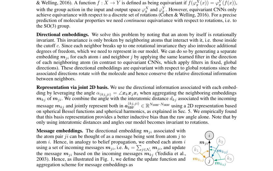
Figure 1: Aggregation scheme for message embeddings.

图 1：消息嵌入的聚合方案。

Message embeddings. The directional embedding ${\bm{m}}_{ji}$ associated with the atom pair $ji$ can be thought of as a message being sent from atom $j$ to atom $i$. Hence, in analogy to belief propagation, we embed each atom $i$ using a set of incoming messages ${\bm{m}}_{ji}$, i.e. ${\bm{h}}_{i}=\sum_{j\in\mathcal{N}_{i}}{\bm{m}}_{ji}$, and update the message ${\bm{m}}_{ji}$ based on the incoming messages ${\bm{m}}_{kj}$ (Yedidia et al., 2003). Hence, as illustrated in Fig. 1, we define the update function and aggregation scheme for message embeddings as

消息嵌入。 与原子对 $ji$ 关联的有向嵌入 ${\bm{m}}_{ji}$ 可视为从原子 $j$ 发往原子 $i$ 的消息。因此，类比信念传播，我们用一组传入消息 ${\bm{m}}_{ji}$ 嵌入每个原子 $i$，即 ${\bm{h}}_{i}=\sum_{j\in\mathcal{N}_{i}}{\bm{m}}_{ji}$，并基于传入消息 ${\bm{m}}_{kj}$ 更新消息 ${\bm{m}}_{ji}$（Yedidia et al., 2003）。于是如图 1 所示，我们把消息嵌入的更新函数与聚合方案定义为

$${\bm{m}}_{ji}^{(l+1)}=f_{\text{update}}({\bm{m}}_{ji}^{(l)},\sum_{k\in\mathcal{N}_{j}\setminus\{i\}}f_{\text{int}}({\bm{m}}_{kj}^{(l)},{\bm{e}}_{\text{RBF}}^{(ji)},{\bm{a}}_{\text{SBF}}^{(kj,ji)})), \tag{4}$$

where ${\bm{e}}_{\text{RBF}}^{(ji)}$ denotes the radial basis function representation of the interatomic distance $d_{ji}$, which will be discussed in Sec. 5. We found this aggregation scheme to not only have a nice analogy to belief propagation, but also to empirically perform better than alternatives. Note that since $f_{\text{int}}$ now incorporates the angle between atom pairs, or bonds, we have enabled our model to directly learn the angular potential $E_{\text{angle}}$, the second term in Eq. 1. Moreover, the message embeddings are essentially embeddings of atom pairs, as used by the provably more powerful GNNs based on higher-order Weisfeiler-Lehman tests of isomorphism. Our model can therefore provably distinguish molecules that a regular GNN cannot (e.g. the previous example of a hexagonal and two triangular molecules) (Morris et al., 2019).

其中 ${\bm{e}}_{\text{RBF}}^{(ji)}$ 表示原子间距离 $d_{ji}$ 的径向基函数表示，将在第 5 节讨论。我们发现该聚合方案不仅与信念传播有漂亮类比，经验表现也优于替代方案。注意：由于 $f_{\text{int}}$ 现已纳入原子对（或键）之间的夹角，模型可直接学习角势 $E_{\text{angle}}$，即式 1 的第二项。此外，消息嵌入本质上是原子对嵌入，正如基于高阶 Weisfeiler-Lehman 同构检验、可证更强的 GNN 所使用的。因此我们的模型可证能区分常规 GNN 无法区分的分子（例如前面六边形与两个三角形分子的例子）（Morris et al., 2019）。

5 Physically based representations

5 基于物理的表示

Representing distances and angles. For the interaction function $f_{\text{int}}$ in Eq. 4 we use a joint representation ${\bm{a}}_{\text{SBF}}^{(kj,ji)}$ of the angles $\alpha_{(kj,ji)}$ between message embeddings and the interatomic distances $d_{kj}=\|{\bm{x}}_{k}-{\bm{x}}_{j}\|_{2}$, as well as a representation ${\bm{e}}_{\text{RBF}}^{(ji)}$ of the distances $d_{ji}$. Earlier works have used a set of Gaussian radial basis functions to represent interatomic distances, with tightly spaced means that are distributed e.g. uniformly (Schütt et al., 2017) or exponentially (Unke & Meuwly, 2019). Similar in spirit to the functional bases used by steerable CNNs (Cohen & Welling, 2017; Cheng et al., 2019) we propose to use an orthogonal basis instead, which reduces redundancy and thus improves parameter efficiency. Furthermore, a basis chosen according to the properties of the modeled system can even provide a helpful inductive bias. We therefore derive a proper basis representation for quantum systems next.

表示距离与角度。 对式 4 中的相互作用函数 $f_{\text{int}}$，我们使用消息嵌入之间夹角 $\alpha_{(kj,ji)}$ 与原子间距离 $d_{kj}=\|{\bm{x}}_{k}-{\bm{x}}_{j}\|_{2}$ 的联合表示 ${\bm{a}}_{\text{SBF}}^{(kj,ji)}$，以及对距离 $d_{ji}$ 的表示 ${\bm{e}}_{\text{RBF}}^{(ji)}$。早期工作用一组高斯径向基函数表示原子间距离，均值紧密排布，例如均匀分布（Schütt et al., 2017）或指数分布（Unke & Meuwly, 2019）。与可转向 CNN 所用函数基的精神类似（Cohen & Welling, 2017; Cheng et al., 2019），我们提出改用正交基，以减少冗余并提升参数效率。此外，按所建模系统性质选取的基甚至可提供有益的归纳偏置。因此我们接下来推导量子系统的恰当基表示。

From Schrödinger to Fourier-Bessel. To construct a basis representation in a principled manner we first consider the space of possible solutions. Our model aims at approximating results of density functional theory (DFT) calculations, i.e. results given by an electron density $\left<\Psi({\bm{d}})|\Psi({\bm{d}})\right>$, with the electron wave function $\Psi({\bm{d}})$ and ${\bm{d}}={\bm{x}}_{k}-{\bm{x}}_{j}$. The solution space of $\Psi({\bm{d}})$ is defined by the time-independent Schrödinger equation $\left(-\frac{\hbar^{2}}{2m}\nabla^{2}+V({\bm{d}})\right)\Psi({\bm{d}})=E\Psi({\bm{d}})$, with constant mass $m$ and energy $E$. We do not know the potential $V({\bm{d}})$ and so choose it in an uninformative way by simply setting it to 0 inside the cutoff distance $c$ (up to which we pass messages between atoms) and to $\infty$ outside. Hence, we arrive at the Helmholtz equation $(\nabla^{2}+k^{2})\Psi({\bm{d}})=0$, with the wave number $k=\frac{\sqrt{2mE}}{\hbar}$ and the boundary condition $\Psi(c)=0$ at the cutoff $c$. Separation of variables in polar coordinates $(d,\alpha,\varphi)$ yields the solution (Griffiths & Schroeter, 2018)

从薛定谔到傅里叶–贝塞尔。 为有原则地构造基表示，我们先考虑可能解的空间。我们的模型旨在逼近密度泛函理论（DFT）计算的结果，即由电子密度 $\left<\Psi({\bm{d}})|\Psi({\bm{d}})\right>$ 给出的结果，其中电子波函数为 $\Psi({\bm{d}})$，${\bm{d}}={\bm{x}}_{k}-{\bm{x}}_{j}$。$\Psi({\bm{d}})$ 的解空间由定态薛定谔方程 $\left(-\frac{\hbar^{2}}{2m}\nabla^{2}+V({\bm{d}})\right)\Psi({\bm{d}})=E\Psi({\bm{d}})$ 定义，质量 $m$ 与能量 $E$ 为常数。我们不知道势 $V({\bm{d}})$，因而以无信息方式选取：在截断距离 $c$ 内（在此范围内原子间传消息）简单置为 0，在外置为 $\infty$。于是得到亥姆霍兹方程 $(\nabla^{2}+k^{2})\Psi({\bm{d}})=0$，波数 $k=\frac{\sqrt{2mE}}{\hbar}$，边界条件在截断 $c$ 处 $\Psi(c)=0$。在极坐标 $(d,\alpha,\varphi)$ 中分离变量得到解（Griffiths & Schroeter, 2018）

$$\Psi(d,\alpha,\varphi)=\sum_{l=0}^{\infty}\sum_{m=-l}^{l}(a_{lm}j_{l}(kd)+b_{lm}y_{l}(kd))Y_{l}^{m}(\alpha,\varphi), \tag{5}$$

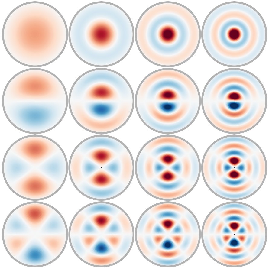
Figure 2: 2D spherical Fourier-Bessel basis $\tilde{a}_{\text{SBF},ln}(d,\alpha)$.

图 2：二维球面傅里叶–贝塞尔基 $\tilde{a}_{\text{SBF},ln}(d,\alpha)$。

with the spherical Bessel functions of the first and second kind $j_{l}$ and $y_{l}$ and the spherical harmonics $Y_{l}^{m}$. As common in physics we only use the regular solutions, i.e. those that do not approach $-\infty$ at the origin, and hence set $b_{lm}=0$. Recall that our first goal is to construct a joint 2D basis for $d_{kj}$ and $\alpha_{(kj,ji)}$, i.e. a function that depends on $d$ and a single angle $\alpha$. To achieve this we set $m=0$ and obtain $\Psi_{\text{SBF}}(d,\alpha)=\sum_{l}a_{l}j_{l}(kd)Y_{l}^{0}(\alpha)$. The boundary conditions are satisfied by setting $k=\frac{z_{ln}}{c}$, where $z_{ln}$ is the $n$-th root of the $l$-order Bessel function, which are precomputed numerically. Normalizing $\Psi_{\text{SBF}}$ inside the cutoff distance $c$ yields the 2D spherical Fourier-Bessel basis $\tilde{{\bm{a}}}_{\text{SBF}}^{(kj,ji)}\in\mathbb{R}^{N_{\text{SHBF}}\cdot N_{\text{SRBF}}}$, which is illustrated in Fig. 3 and defined by

其中 $j_{l}$ 与 $y_{l}$ 为一类与二类球贝塞尔函数，$Y_{l}^{m}$ 为球谐函数。按物理学惯例我们只使用正则解，即在原点不趋于 $-\infty$ 的解，因而令 $b_{lm}=0$。回顾我们的第一个目标是为 $d_{kj}$ 与 $\alpha_{(kj,ji)}$ 构造联合二维基，即依赖 $d$ 与单一角度 $\alpha$ 的函数。为此令 $m=0$，得到 $\Psi_{\text{SBF}}(d,\alpha)=\sum_{l}a_{l}j_{l}(kd)Y_{l}^{0}(\alpha)$。通过令 $k=\frac{z_{ln}}{c}$ 满足边界条件，其中 $z_{ln}$ 为 $l$ 阶贝塞尔函数的第 $n$ 个根，数值预计算得到。在截断距离 $c$ 内归一化 $\Psi_{\text{SBF}}$，得到二维球面傅里叶–贝塞尔基 $\tilde{{\bm{a}}}_{\text{SBF}}^{(kj,ji)}\in\mathbb{R}^{N_{\text{SHBF}}\cdot N_{\text{SRBF}}}$，如图 3 所示，定义为

$$\tilde{a}_{\text{SBF},ln}(d,\alpha)=\sqrt{\frac{2}{c^{3}j_{l+1}^{2}(z_{ln})}}j_{l}(\frac{z_{ln}}{c}d)Y_{l}^{0}(\alpha), \tag{6}$$

with $l\in[0\mathinner{\ldotp\ldotp}N_{\text{SHBF}}-1]$ and $n\in[1\mathinner{\ldotp\ldotp}N_{\text{SRBF}}]$. Our second goal is constructing a radial basis for $d_{ji}$, i.e. a function that solely depends on $d$ and not on the angles $\alpha$ and $\varphi$. We achieve this by setting $l=m=0$ and obtain $\Psi_{\text{RBF}}(d)=aj_{0}(\frac{z_{0,n}}{c}d)$, with roots at $z_{0,n}=n\pi$. Normalizing this function on $[0,c]$ and using $j_{0}(d)=\sin(d)/d$ gives the radial basis $\tilde{{\bm{e}}}_{\text{RBF}}\in\mathbb{R}^{N_{\text{RBF}}}$, as shown in Fig. 3 and defined by

其中 $l\in[0\mathinner{\ldotp\ldotp}N_{\text{SHBF}}-1]$，$n\in[1\mathinner{\ldotp\ldotp}N_{\text{SRBF}}]$。第二个目标是为 $d_{ji}$ 构造径向基，即只依赖 $d$、不依赖角度 $\alpha$ 与 $\varphi$ 的函数。令 $l=m=0$，得到 $\Psi_{\text{RBF}}(d)=aj_{0}(\frac{z_{0,n}}{c}d)$，根在 $z_{0,n}=n\pi$。在 $[0,c]$ 上归一化该函数，并用 $j_{0}(d)=\sin(d)/d$，得到径向基 $\tilde{{\bm{e}}}_{\text{RBF}}\in\mathbb{R}^{N_{\text{RBF}}}$，如图 3 所示，定义为

$$\tilde{e}_{\text{RBF},n}(d)=\sqrt{\frac{2}{c}}\frac{\sin(\frac{n\pi}{c}d)}{d}, \tag{7}$$

with $n\in[1\mathinner{\ldotp\ldotp}N_{\text{RBF}}]$. Both of these bases are purely real-valued and orthogonal in the domain of interest. They furthermore enable us to bound the highest-frequency components by $\omega_{\alpha}\leq\frac{N_{\text{SHBF}}}{2\pi}$, $\omega_{d_{kj}}\leq\frac{N_{\text{SRBF}}}{c}$, and $\omega_{d_{ji}}\leq\frac{N_{\text{RBF}}}{c}$. This restriction is an effective way of regularizing the model and ensures that predictions are stable to small perturbations. We found $N_{\text{SRBF}}=6$ and $N_{\text{RBF}}=16$ radial basis functions to be more than sufficient. Note that $N_{\text{RBF}}$ is 4x lower than PhysNet’s 64 (Unke & Meuwly, 2019) and 20x lower than SchNet’s 300 radial basis functions (Schütt et al., 2017).

其中 $n\in[1\mathinner{\ldotp\ldotp}N_{\text{RBF}}]$。这两种基在感兴趣域上均为纯实值且正交。它们还使我们能把最高频分量界住：$\omega_{\alpha}\leq\frac{N_{\text{SHBF}}}{2\pi}$，$\omega_{d_{kj}}\leq\frac{N_{\text{SRBF}}}{c}$，$\omega_{d_{ji}}\leq\frac{N_{\text{RBF}}}{c}$。该限制是正则化模型的有效方式，并确保预测对小扰动稳定。我们发现 $N_{\text{SRBF}}=6$ 与 $N_{\text{RBF}}=16$ 个径向基函数已绰绰有余。注意 $N_{\text{RBF}}$ 比 PhysNet 的 64（Unke & Meuwly, 2019）低 4 倍，比 SchNet 的 300 个径向基函数（Schütt et al., 2017）低 20 倍。

Continuous cutoff. $\tilde{{\bm{a}}}_{\text{SBF}}^{(kj,ji)}$ and $\tilde{{\bm{e}}}_{\text{RBF}}(d)$ are not twice continuously differentiable due to the step function cutoff at $c$. To alleviate this problem we introduce an envelope function $u(d)$ that has a root of multiplicity 3 at $d=c$, causing the final functions ${\bm{a}}_{\text{RBF}}(d)=u(d)\tilde{{\bm{a}}}_{\text{RBF}}(d)$ and ${\bm{e}}_{\text{RBF}}(d)=u(d)\tilde{{\bm{e}}}_{\text{RBF}}(d)$ and their first and second derivatives to go to 0 at the cutoff. We achieve this with the polynomial

连续截断。 由于在 $c$ 处的阶跃截断，$\tilde{{\bm{a}}}_{\text{SBF}}^{(kj,ji)}$ 与 $\tilde{{\bm{e}}}_{\text{RBF}}(d)$ 并非二阶连续可微。为缓解该问题，我们引入包络函数 $u(d)$，它在 $d=c$ 有三重根，从而使最终函数 ${\bm{a}}_{\text{RBF}}(d)=u(d)\tilde{{\bm{a}}}_{\text{RBF}}(d)$ 与 ${\bm{e}}_{\text{RBF}}(d)=u(d)\tilde{{\bm{e}}}_{\text{RBF}}(d)$ 及其一阶、二阶导数在截断处趋于 0。我们用多项式实现这一点

$$u(d)=1-\frac{(p+1)(p+2)}{2}d^{p}+p(p+2)d^{p+1}-\frac{p(p+1)}{2}d^{p+2}, \tag{8}$$

where $p\in{\mathbb{N}}_{0}$. We did not find the model to be sensitive to different choices of envelope functions and choose $p=6$. Note that using an envelope function causes the bases to lose their orthonormality, which we did not find to be a problem in practice. We furthermore fine-tune the Bessel wave numbers $k_{n}=\frac{n\pi}{c}$ used in $\tilde{{\bm{e}}}_{\text{RBF}}\in\mathbb{R}^{N_{\text{RBF}}}$ via backpropagation after initializing them to these values, which we found to give a small boost in prediction accuracy.

其中 $p\in{\mathbb{N}}_{0}$。我们未发现模型对不同包络函数选择敏感，取 $p=6$。注意使用包络函数会使基失去标准正交性，实践中我们未发现这成问题。此外，在把 $\tilde{{\bm{e}}}_{\text{RBF}}\in\mathbb{R}^{N_{\text{RBF}}}$ 中使用的贝塞尔波数 $k_{n}=\frac{n\pi}{c}$ 初始化为这些值后，我们再经反向传播微调，发现可小幅提升预测精度。

6 Directional Message Passing Neural Network (DimeNet)

6 有向消息传递神经网络（DimeNet）

Figure 4: The DimeNet architecture. $\square$ denotes the layer’s input and $\|$ denotes concatenation. The distances $d_{ji}$ are represented using spherical Bessel functions and the distances $d_{kj}$ and angles $\alpha_{(kj,ji)}$ are jointly represented using a 2D spherical Fourier-Bessel basis. An embedding block generates the inital message embeddings ${\bm{m}}_{ji}$. These embeddings are updated in multiple interaction blocks via directional message passing, which uses the neighboring messages ${\bm{m}}_{kj},k\in\mathcal{N}_{j}\setminus\{i\}$, the 2D representations ${\bm{a}}_{\text{SBF}}^{(kj,ji)}$, and the distance representations ${\bm{e}}_{\text{RBF}}^{(ji)}$. Each block passes the resulting embeddings to an output block, which transforms them using the radial basis ${\bm{e}}_{\text{RBF}}^{(ji)}$ and sums them up per atom. Finally, the outputs of all layers are summed up to generate the prediction.

图 4：DimeNet 架构。$\square$ 表示层的输入，$\|$ 表示拼接。距离 $d_{ji}$ 用球贝塞尔函数表示；距离 $d_{kj}$ 与夹角 $\alpha_{(kj,ji)}$ 用二维球面傅里叶–贝塞尔基联合表示。嵌入块生成初始消息嵌入 ${\bm{m}}_{ji}$。这些嵌入在多个相互作用块中经有向消息传递更新，使用邻近消息 ${\bm{m}}_{kj},k\in\mathcal{N}_{j}\setminus\{i\}$、二维表示 ${\bm{a}}_{\text{SBF}}^{(kj,ji)}$ 与距离表示 ${\bm{e}}_{\text{RBF}}^{(ji)}$。每个块把所得嵌入传给输出块，输出块用径向基 ${\bm{e}}_{\text{RBF}}^{(ji)}$ 变换后按原子求和。最后把所有层的输出相加得到预测。

The Directional Message Passing Neural Network’s (DimeNet) design is based on a streamlined version of the PhysNet architecture (Unke & Meuwly, 2019), in which we have integrated directional message passing and spherical Fourier-Bessel representations. DimeNet generates predictions that are invariant to atom permutations and translation, rotation and inversion of the molecule. DimeNet is suitable both for the prediction of various molecular properties and for molecular dynamics (MD) simulations. It is twice continuously differentiable and able to learn and predict atomic forces via backpropagation, as described in Sec. 3. The predicted forces fulfill energy conservation by construction and are equivariant with respect to permutation and rotation. Model differentiability in combination with basis representations that have bounded maximum frequencies furthermore guarantees smooth predictions that are stable to small deformations. Fig. 4 gives an overview of the architecture.

有向消息传递神经网络（DimeNet）的设计基于精简版 PhysNet 架构（Unke & Meuwly, 2019），其中我们整合了有向消息传递与球面傅里叶–贝塞尔表示。DimeNet 产生的预测对原子置换以及分子的平移、旋转与反演不变。它既适用于多种分子性质预测，也适用于分子动力学（MD）模拟。它二阶连续可微，并能如第 3 节所述经反向传播学习并预测原子力。预测的力由构造满足能量守恒，并对置换与旋转等变。模型可微性与最高频率有界的基表示相结合，还保证预测平滑、对小形变稳定。图 4 给出架构概览。

Embedding block. Atomic numbers are represented by learnable, randomly initialized atom type embeddings ${\bm{h}}_{i}^{(0)}\in\mathbb{R}^{F}$ that are shared across molecules. The first layer generates message embeddings from these and the distance between atoms via

嵌入块。 原子序数由可学习、随机初始化、跨分子共享的原子类型嵌入 ${\bm{h}}_{i}^{(0)}\in\mathbb{R}^{F}$ 表示。第一层由这些嵌入与原子间距离生成消息嵌入：

$${\bm{m}}_{ji}^{(1)}=\sigma([{\bm{h}}_{j}^{(0)}\|{\bm{h}}_{i}^{(0)}\|{\bm{e}}_{\text{RBF}}^{(ji)}]{\bm{W}}+{\bm{b}}), \tag{9}$$

where $\|$ denotes concatenation and the weight matrix ${\bm{W}}$ and bias ${\bm{b}}$ are learnable.

其中 $\|$ 表示拼接，权重矩阵 ${\bm{W}}$ 与偏置 ${\bm{b}}$ 可学习。

Interaction block. The embedding block is followed by multiple stacked interaction blocks. This block implements $f_{\text{int}}$ and $f_{\text{update}}$ of Eq. 4 as shown in Fig. 4. Note that the 2D representation ${\bm{a}}_{\text{SBF}}^{(kj,ji)}$ is first transformed into an $N_{\text{bilinear}}$-dimensional representation via a linear layer. The main purpose of this is to make the dimensionality of ${\bm{a}}_{\text{SBF}}^{(kj,ji)}$ independent of the subsequent bilinear layer, which uses a comparatively large $N_{\text{bilinear}}\times F\times F$-dimensional weight tensor. We have also experimented with using a bilinear layer for the radial basis representation, but found that the element-wise multiplication ${\bm{e}}_{\text{RBF}}^{(ji)}{\bm{W}}\odot{\bm{m}}_{kj}$ performs better, which suggests that the 2D representations require more complex transformations than radial information alone. The interaction block transforms each message embedding ${\bm{m}}_{ji}$ using multiple residual blocks, which are inspired by ResNet (He et al., 2016) and consist of two stacked dense layers and a skip connection.

相互作用块。 嵌入块之后是多个堆叠的相互作用块。该块实现式 4 的 $f_{\text{int}}$ 与 $f_{\text{update}}$，如图 4 所示。注意二维表示 ${\bm{a}}_{\text{SBF}}^{(kj,ji)}$ 先经线性层变换为 $N_{\text{bilinear}}$ 维表示。主要目的是使 ${\bm{a}}_{\text{SBF}}^{(kj,ji)}$ 的维数独立于后续双线性层，后者使用相对较大的 $N_{\text{bilinear}}\times F\times F$ 维权重张量。我们也尝试过对径向基表示使用双线性层，但发现逐元素乘法 ${\bm{e}}_{\text{RBF}}^{(ji)}{\bm{W}}\odot{\bm{m}}_{kj}$ 表现更好，这表明二维表示需要比仅径向信息更复杂的变换。相互作用块用多个残差块变换每个消息嵌入 ${\bm{m}}_{ji}$；残差块受 ResNet（He et al., 2016）启发，由两个堆叠稠密层与一条跳跃连接组成。

Output block. The message embeddings after each block (including the embedding block) are passed to an output block. The output block transforms each message embedding ${\bm{m}}_{ji}$ using the radial basis ${\bm{e}}_{\text{RBF}}^{(ji)}$, which ensures continuous differentiability and slightly improves performance. Afterwards the incoming messages are summed up per atom $i$ to obtain ${\bm{h}}_{i}=\sum_{j}{\bm{m}}_{ji}$, which is then transformed using multiple dense layers to generate the atom-wise output $t_{i}^{(l)}$. These outputs are then summed up to obtain the final prediction $t=\sum_{i}\sum_{l}t_{i}^{(l)}$.

输出块。 每个块（含嵌入块）之后的消息嵌入被送入输出块。输出块用径向基 ${\bm{e}}_{\text{RBF}}^{(ji)}$ 变换每个消息嵌入 ${\bm{m}}_{ji}$，这保证连续可微并略微提升表现。随后按原子 $i$ 对传入消息求和得到 ${\bm{h}}_{i}=\sum_{j}{\bm{m}}_{ji}$，再经多个稠密层变换生成原子级输出 $t_{i}^{(l)}$。这些输出再相加得到最终预测 $t=\sum_{i}\sum_{l}t_{i}^{(l)}$。

Continuous differentiability. Multiple model choices were necessary to achieve twice continuous model differentiability. First, DimeNet uses the self-gated Swish activation function $\sigma(x)=x\cdot\text{sigmoid}(x)$ (Ramachandran et al., 2018) instead of a regular ReLU activation function. Second, we multiply the radial basis functions $\tilde{{\bm{e}}}_{\text{RBF}}(d)$ with an envelope function $u(d)$ that has a root of multiplicity 3 at the cutoff $c$. Finally, DimeNet does not use any auxiliary data but relies on atom types and positions alone.

连续可微性。 为实现二阶连续可微，做了多项模型选择。第一，DimeNet 使用自门控 Swish 激活 $\sigma(x)=x\cdot\text{sigmoid}(x)$（Ramachandran et al., 2018），而非常规 ReLU。第二，我们把径向基函数 $\tilde{{\bm{e}}}_{\text{RBF}}(d)$ 乘以在截断 $c$ 有三重根的包络函数 $u(d)$。最后，DimeNet 不使用任何辅助数据，仅依赖原子类型与位置。

7 Experiments

7 实验

Models. For hyperparameter choices and training setup see Appendix B. We use 6 state-of-the-art models for comparison: SchNet (Schütt et al., 2017), PhysNet (results based on the reference implementation) (Unke & Meuwly, 2019), provably powerful graph networks (PPGN, results provided by the original authors) (Maron et al., 2019), MEGNet-simple (without auxiliary information) (Chen et al., 2019a), Cormorant (Anderson et al., 2019), and symmetrized gradient-domain machine learning (sGDML) (Chmiela et al., 2018). Note that sGDML cannot be used for QM9 since it can only be trained on a single molecule.

模型。 超参选择与训练设置见附录 B。我们用 6 个当时最优模型作比较：SchNet（Schütt et al., 2017）、PhysNet（结果基于参考实现）（Unke & Meuwly, 2019）、可证强大的图网络（PPGN，结果由原作者提供）（Maron et al., 2019）、MEGNet-simple（无辅助信息）（Chen et al., 2019a）、Cormorant（Anderson et al., 2019），以及对称化梯度域机器学习（sGDML）（Chmiela et al., 2018）。注意 sGDML 不能用于 QM9，因为它只能在单个分子上训练。

Target	Unit	PPGN	SchNet	PhysNet	MEGNet-s	Cormorant	DimeNet
$\mu$	$\mathrm{D}$	$0.047$	$0.033$	$0.0529$	$0.05$	$0.13$	$0.0286$
$\alpha$	$\mathrm{a}$	$0.131$	$0.235$	$0.0615$	$0.081$	$0.092$	$0.0469$
$\epsilon_{\text{HOMO}}$	$\mathrm{meV}$	$40.3$	$41$	$32.9$	$43$	$36$	$27.8$
$\epsilon_{\text{LUMO}}$	$\mathrm{meV}$	$32.7$	$34$	$24.7$	$44$	$36$	$19.7$
$\Delta\epsilon$	$\mathrm{meV}$	$60.0$	$63$	$42.5$	$66$	$60$	$34.8$
$\left<R^{2}\right>$	$\mathrm{a}$	$0.592$	$0.073$	$0.765$	$0.302$	$0.673$	$0.331$
ZPVE	$\mathrm{meV}$	$3.12$	$1.7$	$1.39$	$1.43$	$1.98$	$1.29$
$U_{0}$	$\mathrm{meV}$	$36.8$	$14$	$8.15$	$12$	$28$	$8.02$
$U$	$\mathrm{meV}$	$36.8$	$19$	$8.34$	$13$	-	$7.89$
$H$	$\mathrm{meV}$	$36.3$	$14$	$8.42$	$12$	-	$8.11$
$G$	$\mathrm{meV}$	$36.4$	$14$	$9.40$	$12$	-	$8.98$
$c_{\text{v}}$	$\frac{\mathrm{cal}}{\mathrm{mol}\text{\,}\mathrm{K}}$	$0.055$	$0.033$	$0.0280$	$0.029$	$0.031$	$0.0249$
std. MAE	$\mathrm{\%}$	$1.84$	$1.76$	$1.37$	$1.80$	$2.14$	$1.05$
logMAE	-	$-4.64$	$-5.17$	$-5.35$	$-5.17$	$-4.75$	$-5.57$

Table 1: MAE on QM9. DimeNet sets the state of the art on 11 targets, outperforming the second-best model on average by $31\text{\,}\mathrm{\%}$ (mean std. MAE).

Target	Unit	PPGN	SchNet	PhysNet	MEGNet-s	Cormorant	DimeNet
$\mu$	$\mathrm{D}$	$0.047$	$0.033$	$0.0529$	$0.05$	$0.13$	$0.0286$
$\alpha$	$\mathrm{a}$	$0.131$	$0.235$	$0.0615$	$0.081$	$0.092$	$0.0469$
$\epsilon_{\text{HOMO}}$	$\mathrm{meV}$	$40.3$	$41$	$32.9$	$43$	$36$	$27.8$
$\epsilon_{\text{LUMO}}$	$\mathrm{meV}$	$32.7$	$34$	$24.7$	$44$	$36$	$19.7$
$\Delta\epsilon$	$\mathrm{meV}$	$60.0$	$63$	$42.5$	$66$	$60$	$34.8$
$\left<R^{2}\right>$	$\mathrm{a}$	$0.592$	$0.073$	$0.765$	$0.302$	$0.673$	$0.331$
ZPVE	$\mathrm{meV}$	$3.12$	$1.7$	$1.39$	$1.43$	$1.98$	$1.29$
$U_{0}$	$\mathrm{meV}$	$36.8$	$14$	$8.15$	$12$	$28$	$8.02$
$U$	$\mathrm{meV}$	$36.8$	$19$	$8.34$	$13$	-	$7.89$
$H$	$\mathrm{meV}$	$36.3$	$14$	$8.42$	$12$	-	$8.11$
$G$	$\mathrm{meV}$	$36.4$	$14$	$9.40$	$12$	-	$8.98$
$c_{\text{v}}$	$\frac{\mathrm{cal}}{\mathrm{mol}\text{\,}\mathrm{K}}$	$0.055$	$0.033$	$0.0280$	$0.029$	$0.031$	$0.0249$
std. MAE	$\mathrm{\%}$	$1.84$	$1.76$	$1.37$	$1.80$	$2.14$	$1.05$
logMAE	-	$-4.64$	$-5.17$	$-5.35$	$-5.17$	$-4.75$	$-5.57$

表 1：QM9 上的 MAE。DimeNet 在 11 个目标上刷新当时最优，平均 std. MAE 优于次优模型 $31\text{\,}\mathrm{\%}$。

QM9. We test DimeNet’s performance for predicting molecular properties using the common QM9 benchmark (Ramakrishnan et al., 2014). It consists of roughly $130\,000$ molecules in equilibrium with up to 9 heavy C, O, N, and F atoms. We use $110\,000$ molecules in the training, $10\,000$ in the validation and $10\,831$ in the test set. We only use the atomization energy for $U_{0}$, $U$, $H$, and $G$, i.e. subtract the atomic reference energies, which are constant per atom type, and perform the training using $\mathrm{eV}$. In Table 1 we report the mean absolute error (MAE) of each target and the overall mean standardized MAE (std. MAE) and mean standardized logMAE (for details see Appendix C). We predict $\Delta\epsilon$ simply by taking $\epsilon_{\text{LUMO}}-\epsilon_{\text{HOMO}}$, since it is calculated in exactly this way by DFT calculations. We train a separate model for each target, which significantly improves results compared to training a single shared model for all targets (see App. E). DimeNet sets the new state of the art on 11 out of 12 targets and decreases mean std. MAE by $31\text{\,}\mathrm{\%}$ and mean logMAE by $0.22$ compared to the second-best model.

QM9。 我们用常见的 QM9 基准（Ramakrishnan et al., 2014）测试 DimeNet 预测分子性质的表现。它包含约 $130\,000$ 个平衡态分子，最多 9 个重原子 C、O、N、F。我们用 $110\,000$ 个分子训练、$10\,000$ 验证、$10\,831$ 测试。对 $U_{0}$、$U$、$H$ 与 $G$ 我们只用原子化能，即减去按原子类型恒定的原子参考能量，并以 $\mathrm{eV}$ 训练。表 1 报告各目标平均绝对误差（MAE），以及总体平均标准化 MAE（std. MAE）与平均标准化 logMAE（细节见附录 C）。我们简单用 $\epsilon_{\text{LUMO}}-\epsilon_{\text{HOMO}}$ 预测 $\Delta\epsilon$，因为 DFT 计算正是如此得到它。我们为每个目标训练单独模型，相对为全部目标训练单一共享模型显著提升结果（见附录 E）。DimeNet 在 12 个目标中的 11 个上刷新当时最优，相对次优模型把平均 std. MAE 降低 $31\text{\,}\mathrm{\%}$、平均 logMAE 降低 $0.22$。

		sGDML	SchNet	DimeNet
Aspirin	Energy	$0.19$	$0.37$	$0.204$
Forces	$0.68$	$1.35$	$0.499$
Benzene	Energy	$0.10$	$0.08$	$0.078$
Forces	$0.06$	$0.31$	$0.187$
Ethanol	Energy	$0.07$	$0.08$	$0.064$
Forces	$0.33$	$0.39$	$0.230$
Malonaldehyde	Energy	$0.10$	$0.13$	$0.104$
Forces	$0.41$	$0.66$	$0.383$
Naphthalene	Energy	$0.12$	$0.16$	$0.122$
Forces	$0.11$	$0.58$	$0.215$
Salicylic acid	Energy	$0.12$	$0.20$	$0.134$
Forces	$0.28$	$0.85$	$0.374$
Toluene	Energy	$0.10$	$0.12$	$0.102$
Forces	$0.14$	$0.57$	$0.216$
Uracil	Energy	$0.11$	$0.14$	$0.115$
Forces	$0.24$	$0.56$	$0.301$
std. MAE ($\mathrm{\%}$)	Energy	$2.53$	$3.32$	$2.49$
Forces	$1.01$	$2.38$	$1.10$

Variation	$\frac{\text{MAE}}{\text{MAE DimeNet}}$	$\Delta$logMAE
Gaussian RBF	$110\text{\,}\mathrm{\%}$	$0.10$
$N_{\text{SHBF}}=1$	$126\text{\,}\mathrm{\%}$	$0.11$
Node embeddings	$168\text{\,}\mathrm{\%}$	$0.45$

Figure 5: MAE on MD17 using $1000$ training samples (energies in $\frac{\mathrm{kcal}}{\mathrm{mol}}$, forces in $\frac{\mathrm{kcal}}{\mathrm{mol}\text{\,}\mathrm{\SIUnitSymbolAngstrom}}$). DimeNet outperforms SchNet by a large margin and performs roughly on par with sGDML.

References

参考文献
Anderson et al. (2019) Brandon M. Anderson, Truong-Son Hy, and Risi Kondor. Cormorant: Covariant Molecular Neural Networks. In NeurIPS , 2019.
Bartók et al. (2010) Albert P. Bartók, Mike C. Payne, Risi Kondor, and Gábor Csányi. Gaussian Approximation Potentials: The Accuracy of Quantum Mechanics, without the Electrons. Physical Review Letters , 104(13):136403, April 2010.
Bartók et al. (2013) Albert P. Bartók, Risi Kondor, and Gábor Csányi. On representing chemical environments. Physical Review B , 87(18):184115, May 2013.
Bartók et al. (2017) Albert P. Bartók, Sandip De, Carl Poelking, Noam Bernstein, James R. Kermode, Gábor Csányi, and Michele Ceriotti. Machine learning unifies the modeling of materials and molecules. Science Advances , 3(12):e1701816, December 2017.
Baskin et al. (1997) Igor I. Baskin, Vladimir A. Palyulin, and Nikolai S. Zefirov. A Neural Device for Searching Direct Correlations between Structures and Properties of Chemical Compounds. Journal of Chemical Information and Computer Sciences , 37(4):715–721, July 1997.
Behler & Parrinello (2007) Jörg Behler and Michele Parrinello. Generalized Neural-Network Representation of High-Dimensional Potential-Energy Surfaces. Physical Review Letters , 98(14):146401, April 2007.
Chen et al. (2019a) Chi Chen, Weike Ye, Yunxing Zuo, Chen Zheng, and Shyue Ping Ong. Graph Networks as a Universal Machine Learning Framework for Molecules and Crystals. Chemistry of Materials , 31(9):3564–3572, May 2019a.
Chen et al. (2019b) Zhengdao Chen, Lisha Li, and Joan Bruna. Supervised Community Detection with Line Graph Neural Networks. In ICLR , 2019b.
Cheng et al. (2019) Xiuyuan Cheng, Qiang Qiu, A. Robert Calderbank, and Guillermo Sapiro. RotDCF: Decomposition of Convolutional Filters for Rotation-Equivariant Deep Networks. In ICLR , 2019.
Chmiela et al. (2017) Stefan Chmiela, Alexandre Tkatchenko, Huziel E. Sauceda, Igor Poltavsky, Kristof T. Schütt, and Klaus-Robert Müller. Machine learning of accurate energy-conserving molecular force fields. Science Advances , 3(5):e1603015, May 2017.
Chmiela et al. (2018) Stefan Chmiela, Huziel E. Sauceda, Klaus-Robert Müller, and Alexandre Tkatchenko. Towards exact molecular dynamics simulations with machine-learned force fields. Nature Communications , 9(1):1–10, September 2018.
Cohen & Welling (2016) Taco Cohen and Max Welling. Group Equivariant Convolutional Networks. In ICML , 2016.
Cohen et al. (2019) Taco Cohen, Maurice Weiler, Berkay Kicanaoglu, and Max Welling. Gauge Equivariant Convolutional Networks and the Icosahedral CNN. In ICML , 2019.
Cohen & Welling (2017) Taco S. Cohen and Max Welling. Steerable CNNs. In ICLR , 2017.
Cohen et al. (2018) Taco S. Cohen, Mario Geiger, Jonas Köhler, and Max Welling. Spherical CNNs. In ICLR , 2018.
Duvenaud et al. (2015) David K. Duvenaud, Dougal Maclaurin, Jorge Aguilera-Iparraguirre, Rafael Gómez-Bombarelli, Timothy Hirzel, Alán Aspuru-Guzik, and Ryan P. Adams. Convolutional Networks on Graphs for Learning Molecular Fingerprints. In NIPS , 2015.
Faber et al. (2017) Felix A. Faber, Luke Hutchison, Bing Huang, Justin Gilmer, Samuel S. Schoenholz, George E. Dahl, Oriol Vinyals, Steven Kearnes, Patrick F. Riley, and O. Anatole von Lilienfeld. Machine learning prediction errors better than DFT accuracy. CoRR , 1702.05532, February 2017.
Gasteiger et al. (2019) Johannes Gasteiger, Aleksandar Bojchevski, and Stephan Günnemann. Predict then Propagate: Graph Neural Networks Meet Personalized PageRank. In ICLR , 2019.
Gilmer et al. (2017) Justin Gilmer, Samuel S. Schoenholz, Patrick F. Riley, Oriol Vinyals, and George E. Dahl. Neural Message Passing for Quantum Chemistry. In ICML , 2017.
Gori et al. (2005) M. Gori, G. Monfardini, and F. Scarselli. A new model for learning in graph domains. In IEEE International Joint Conference on Neural Networks , July 2005.
Griffiths & Schroeter (2018) David J. Griffiths and Darrell F. Schroeter. Introduction to Quantum Mechanics . 3 edition, August 2018.
He et al. (2016) Kaiming He, Xiangyu Zhang, Shaoqing Ren, and Jian Sun. Deep Residual Learning for Image Recognition. In CVPR , 2016.
Hy et al. (2018) Truong Son Hy, Shubhendu Trivedi, Horace Pan, Brandon M. Anderson, and Risi Kondor. Predicting molecular properties with covariant compositional networks. The Journal of Chemical Physics , 148(24):241745, June 2018.
Ingraham et al. (2019) John Ingraham, Vikas K. Garg, Regina Barzilay, and Tommi S. Jaakkola. Generative Models for Graph-Based Protein Design. In ICLR workshop , 2019.
Jørgensen et al. (2018) Peter Bjørn Jørgensen, Karsten Wedel Jacobsen, and Mikkel N. Schmidt. Neural Message Passing with Edge Updates for Predicting Properties of Molecules and Materials. CoRR , 1806.03146, 2018.
Kipf & Welling (2017) Thomas N. Kipf and Max Welling. Semi-Supervised Classification with Graph Convolutional Networks. In ICLR , 2017.
Kondor et al. (2018) Risi Kondor, Zhen Lin, and Shubhendu Trivedi. Clebsch-Gordan Nets: a Fully Fourier Space Spherical Convolutional Neural Network. In NeurIPS , 2018.
Leach (2001) Andrew R. Leach. Molecular Modelling: Principles and Applications . 2001.
Maron et al. (2019) Haggai Maron, Heli Ben-Hamu, Hadar Serviansky, and Yaron Lipman. Provably Powerful Graph Networks. In NeurIPS , 2019.
Morris et al. (2019) Christopher Morris, Martin Ritzert, Matthias Fey, William L. Hamilton, Jan Eric Lenssen, Gaurav Rattan, and Martin Grohe. Weisfeiler and Leman Go Neural: Higher-Order Graph Neural Networks. In AAAI , 2019.
Noether (1918) Emmy Noether. Invariante Variationsprobleme. Nachrichten von der Gesellschaft der Wissenschaften zu Göttingen, Mathematisch-Physikalische Klasse , 1918:235–257, 1918.
Pukrittayakamee et al. (2009) A. Pukrittayakamee, M. Malshe, M. Hagan, L. M. Raff, R. Narulkar, S. Bukkapatnum, and R. Komanduri. Simultaneous fitting of a potential-energy surface and its corresponding force fields using feedforward neural networks. The Journal of Chemical Physics , 130(13):134101, April 2009.
Ramachandran et al. (2018) Prajit Ramachandran, Barret Zoph, and Quoc V. Le. Searching for Activation Functions. In ICLR workshop , 2018.
Ramakrishnan et al. (2014) Raghunathan Ramakrishnan, Pavlo O. Dral, Matthias Rupp, and O. Anatole von Lilienfeld. Quantum chemistry structures and properties of 134 kilo molecules. Scientific Data , 1(1):1–7, August 2014.
Ravanbakhsh et al. (2017) Siamak Ravanbakhsh, Jeff G. Schneider, and Barnabás Póczos. Equivariance Through Parameter-Sharing. In ICML , 2017.
Reddi et al. (2018) Sashank J. Reddi, Satyen Kale, and Sanjiv Kumar. On the Convergence of Adam and Beyond. In ICLR , 2018.
Scarselli et al. (2009) F. Scarselli, M. Gori, Ah Chung Tsoi, M. Hagenbuchner, and G. Monfardini. The Graph Neural Network Model. IEEE Transactions on Neural Networks , 20(1):61–80, January 2009.
Schütt et al. (2017) Kristof Schütt, Pieter-Jan Kindermans, Huziel Enoc Sauceda Felix, Stefan Chmiela, Alexandre Tkatchenko, and Klaus-Robert Müller. SchNet: A continuous-filter convolutional neural network for modeling quantum interactions. In NIPS , 2017.
Sperduti & Starita (1997) A. Sperduti and A. Starita. Supervised neural networks for the classification of structures. IEEE Transactions on Neural Networks , 8(3):714–735, May 1997.
Thomas et al. (2018) Nathaniel Thomas, Tess Smidt, Steven M. Kearnes, Lusann Yang, Li Li, Kai Kohlhoff, and Patrick Riley. Tensor Field Networks: Rotation- and Translation-Equivariant Neural Networks for 3D Point Clouds. CoRR , 1802.08219, 2018.
Unke & Meuwly (2019) Oliver T. Unke and Markus Meuwly. PhysNet: A Neural Network for Predicting Energies, Forces, Dipole Moments, and Partial Charges. Journal of Chemical Theory and Computation , 15(6):3678–3693, June 2019.
Weiler et al. (2018) Maurice Weiler, Mario Geiger, Max Welling, Wouter Boomsma, and Taco Cohen. 3D Steerable CNNs: Learning Rotationally Equivariant Features in Volumetric Data. In NeurIPS , 2018.
Wu et al. (2018) Zhenqin Wu, Bharath Ramsundar, Evan N. Feinberg, Joseph Gomes, Caleb Geniesse, Aneesh S. Pappu, Karl Leswing, and Vijay Pande. MoleculeNet: a benchmark for molecular machine learning. Chemical Science , 9(2):513–530, 2018.
Xu et al. (2019) Keyulu Xu, Weihua Hu, Jure Leskovec, and Stefanie Jegelka. How Powerful are Graph Neural Networks? In ICLR , 2019.
Yedidia et al. (2003) Jonathan S Yedidia, William T Freeman, and Yair Weiss. Understanding belief propagation and its generalizations. In Exploring artificial intelligence in the new millennium , volume 8, pp. 236–239. 2003.
Zambaldi et al. (2019) Vinícius Flores Zambaldi, David Raposo, Adam Santoro, Victor Bapst, Yujia Li, Igor Babuschkin, Karl Tuyls, David P. Reichert, Timothy P. Lillicrap, Edward Lockhart, Murray Shanahan, Victoria Langston, Razvan Pascanu, Matthew Botvinick, Oriol Vinyals, and Peter W. Battaglia. Deep reinforcement learning with relational inductive biases. In ICLR , 2019.
Appendix A Indistinguishable molecules
附录 A 不可区分的分子
Figure 8: A standard non-directional GNN cannot distinguish between a hexagonal (left) and two triangular molecules (right) with the same bond lengths, since the neighborhood of each atom is exactly the same. An example of this would be Cyclohexane and two Cyclopropane molecules with slightly stretched bonds, when the GNN either uses the molecular graph or a cutoff distance of 2.5\text{,}\mathrm{\SIUnitSymbolAngstrom}$$. Directional message passing solves this problem by considering the direction of each bond.
图 8:标准无向 GNN 无法区分键长相同的六边形分子(左)与两个三角形分子(右),因为每个原子的邻域完全相同。例如环己烷与两个键略被拉长的环丙烷,当 GNN 使用分子图或截断距离 2.5\text{,}\mathrm{\SIUnitSymbolAngstrom}$$ 时即如此。有向消息传递通过考虑每条键的方向解决该问题。
Appendix B Experimental setup
附录 B 实验设置
The model architecture and hyperparameters were optimized using the QM9 validation set. We use 6 stacked interaction blocks and embeddings of size throughout the model. For the basis functions we choose and . For the weight tensor in the interaction block we use . We did not find the model to be very sensitive to these values as long as they were large enough (i.e. at least 4).
模型架构与超参在 QM9 验证集上优化。我们使用 6 个堆叠相互作用块,模型全程嵌入大小 。基函数取 ,。相互作用块中的权重张量取 。只要这些值足够大(即至少 4),我们未发现模型对其非常敏感。
We found the cutoff 5\text{,}\mathrm{\SIUnitSymbolAngstrom}$$ and the learning rate to be rather important hyperparameters. We optimized the model using AMSGrad (Reddi et al., 2018) with 32 molecules per mini-batch. We use a linear learning rate warm-up over steps and an exponential decay with ratio every steps. The model weights for validation and test were obtained using an exponential moving average (EMA) with decay rate . For MD17 we use the loss function from Eq. 2 with force weight , like previous models Schütt et al. (2017). Note that presents a trade-off between energy and force accuracy. It should be chosen rather high since the forces determine the dynamics of the chemical system (Unke & Meuwly, 2019). We use early stopping on the validation loss. On QM9 we train for at most and on MD17 for at most steps.
我们发现截断 5\text{,}\mathrm{\SIUnitSymbolAngstrom}$$ 与学习率 是相当重要的超参。用 AMSGrad(Reddi et al., 2018)优化,每小批量 32 个分子。学习率在 步内线性预热,并以每 步比率 指数衰减。验证与测试用的模型权重由衰减率 的指数滑动平均(EMA)得到。对 MD17 使用式 2 的损失函数,力权重 ,与先前模型 Schütt et al. (2017) 一致。注意 在能量与力精度之间做权衡;由于力决定化学系统动力学,应取得偏高(Unke & Meuwly, 2019)。我们在验证损失上早停。QM9 最多训练 步,MD17 最多 步。
Appendix C Summary statistics
附录 C 汇总统计
We summarize the results across different targets using the mean standardized MAE
我们用平均标准化 MAE 汇总不同目标上的结果
and the mean standardized logMAE
以及平均标准化 logMAE
with target index , number of targets , dataset size , ground truth values , model , inputs and , and standard deviation of . Std. MAE reflects the average error compared to the standard deviation of each target. Since this error is dominated by a few difficult targets (e.g. ) we also report logMAE, which reflects every relative improvement equally but is sensitive to outliers, such as SchNet’s result on .
其中目标索引 ,目标数 ,数据集大小 ,真实值 ,模型 ,输入 与 ,以及 的标准差 。Std. MAE 反映相对各目标标准差的平均误差。由于该误差由少数困难目标主导(如 ),我们也报告 logMAE:它对每次相对改进同等反映,但对离群值敏感,例如 SchNet 在 上的结果。
Appendix D DimeNet filters
附录 D DimeNet 滤波器
To illustrate the filters learned by DimeNet we separate the spatial dependency in the interaction function via
为说明 DimeNet 学到的滤波器,我们把相互作用函数 中的空间依赖分离为
The filters and are given by
滤波器 与 由下式给出
where , , and are learned weight matrices/tensors, is the radial basis representation, and is the 2D spherical Fourier-Bessel representation. Fig. 7 shows how the first 15 elements of vary with and when choosing the tensor slice (with at the top of the figure).
其中 、 与 为学得的权重矩阵/张量, 为径向基表示, 为二维球面傅里叶–贝塞尔表示。图 7 展示取张量切片 时, 的前 15 个元素如何随 与 变化(图顶部 )。
Appendix E Multi-target results