DiffWave: A Versatile Diffusion Model for Audio Synthesis
DiffWave: A Versatile Diffusion Model for Audio Synthesis
DiffWave:面向音频合成的通用扩散模型
Zhifeng Kong Thanks: Contributed to the work during an internship at Baidu Research, USA. Affiliation: Computer Science and Engineering, UCSD Email: z4kong@eng.ucsd.edu Wei Ping Affiliation: NVIDIA Affiliation: wping@nvidia.com Jiaji Huang Kexin Zhao Affiliation: Baidu Research Email: {huangjiaji,kexinzhao}@baidu.com Bryan Catanzaro Affiliation: NVIDIA Affiliation: bcatanzaro@nvidia.com
Abstract
摘要
In this work, we propose DiffWave, a versatile diffusion probabilistic model for conditional and unconditional waveform generation. The model is non-autoregressive, and converts the white noise signal into structured waveform through a Markov chain with a constant number of steps at synthesis. It is efficiently trained by optimizing a variant of variational bound on the data likelihood. DiffWave produces high-fidelity audio in different waveform generation tasks, including neural vocoding conditioned on mel spectrogram, class-conditional generation, and unconditional generation. We demonstrate that DiffWave matches a strong WaveNet vocoder in terms of speech quality (MOS: 4.44 versus 4.43), while synthesizing orders of magnitude faster. In particular, it significantly outperforms autoregressive and GAN-based waveform models in the challenging unconditional generation task in terms of audio quality and sample diversity from various automatic and human evaluations. [^1]
本文提出 DiffWave:一种可同时做条件与无条件波形生成的通用扩散概率模型。模型非自回归,在合成时以固定步数的马尔可夫链把白噪声转成结构化波形;训练则优化数据似然的一类变分下界变体。DiffWave 在多种波形生成任务上都能给出高保真音频,包括以梅尔谱为条件的神经声码、类别条件生成与无条件生成。语音质量上,它与强 WaveNet 声码器相当(MOS:4.44 对 4.43),合成速度却高出几个数量级。尤其在颇具挑战的无条件生成上,自动评测与听感评测都显示:相对自回归与基于 GAN 的波形模型,DiffWave 在音质与样本多样性上明显更优。[^1]
1 Introduction
1 引言
Deep generative models have produced high-fidelity raw audio in speech synthesis and music generation. In previous work, likelihood-based models, including autoregressive models (van den Oord et al. 2016; Kalchbrenner et al. 2018; Mehri et al. 2017) and flow-based models (Prenger et al. 2019; Ping et al. 2020; Kim et al. 2019), have predominated in audio synthesis because of the simple training objective and superior ability of modeling the fine details of waveform in real data. There are other waveform models, which often require auxiliary losses for training, such as flow-based models trained by distillation (van den Oord et al. 2018; Ping et al. 2019), variational auto-encoder (VAE) based model (Peng et al. 2020), and generative adversarial network (GAN) based models (Kumar et al. 2019; Bińkowski et al. 2020; Yamamoto et al. 2020).
深度生成模型已能在语音合成与音乐生成中产出高保真原始音频。既往工作里,基于似然的模型——含自回归模型(van den Oord et al. 2016;Kalchbrenner et al. 2018;Mehri et al. 2017)与基于流的模型(Prenger et al. 2019;Ping et al. 2020;Kim et al. 2019)——因训练目标简洁、又能刻画真实波形细部,长期主导音频合成。另有一些波形模型常需辅助损失,例如经蒸馏训练的流模型(van den Oord et al. 2018;Ping et al. 2019)、基于变分自编码器(VAE)的模型(Peng et al. 2020),以及基于生成对抗网络(GAN)的模型(Kumar et al. 2019;Bińkowski et al. 2020;Yamamoto et al. 2020)。
Most of previous waveform models focus on audio synthesis with informative local conditioner (e.g., mel spectrogram or aligned linguistic features), with only a few exceptions for unconditional generation (Mehri et al. 2017; Donahue et al. 2019). It has been noticed that autoregressive models (e.g., WaveNet) tend to generate made-up word-like sounds (van den Oord et al. 2016), or inferior samples (Donahue et al. 2019) under unconditional settings. This is because very long sequences need to be generated (e.g., 16,000 time-steps for one second speech) without any conditional information.
此前多数波形模型聚焦于带丰富局部条件(如梅尔谱或对齐语言学特征)的音频合成,无条件生成仅有少数例外(Mehri et al. 2017;Donahue et al. 2019)。已有观察指出:自回归模型(如 WaveNet)在无条件设定下容易发出虚构的词样声音(van den Oord et al. 2016),或质量较差的样本(Donahue et al. 2019)。原因在于:没有任何条件信息时,仍需生成极长序列(例如一秒语音对应 16,000 个时间步)。
Diffusion probabilistic models (diffusion models for brevity) are a class of promising generative models, which use a Markov chain to gradually convert a simple distribution (e.g., isotropic Gaussian) into complicated data distribution (Sohl-Dickstein et al. 2015; Goyal et al. 2017; Ho et al. 2020). Although the data likelihood is intractable, diffusion models can be efficiently trained by optimizing the variational lower bound (ELBO). Most recently, a certain parameterization has been shown successful in image synthesis (Ho et al. 2020), which is connected with denoising score matching (Song & Ermon 2019). Diffusion models can use a diffusion (noise-adding) process without learnable parameters to obtain the “whitened” latents from training data. Therefore, no additional neural networks are required for training in contrast to other models (e.g., the encoder in VAE (Kingma & Welling 2014) or the discriminator in GAN (Goodfellow et al. 2014)). This avoids the challenging “posterior collapse” or “mode collapse” issues stemming from the joint training of two networks, and hence is valuable for high-fidelity audio synthesis.
扩散概率模型(简称扩散模型)是一类有潜力的生成模型:用马尔可夫链把简单分布(如各向同性高斯)逐步转成复杂数据分布(Sohl-Dickstein et al. 2015;Goyal et al. 2017;Ho et al. 2020)。数据似然虽不可积,但可通过优化变分下界(ELBO)高效训练。最近,一种参数化在图像合成上取得成功(Ho et al. 2020),并与去噪分数匹配相连(Song & Ermon 2019)。扩散模型可用不含可学习参数的扩散(加噪)过程,从训练数据得到「白化」隐变量,因而相对其他模型(如 VAE 的编码器(Kingma & Welling 2014)或 GAN 的判别器(Goodfellow et al. 2014))不必再训额外网络。这避开了双网络联合训练带来的「后验坍塌」或「模式坍塌」,对高保真音频合成很有价值。
In this work, we propose DiffWave, a versatile diffusion probabilistic model for raw audio synthesis. DiffWave has several advantages over previous work: i) It is non-autoregressive thus can synthesize high-dimensional waveform in parallel. ii) It is flexible as it does not impose any architectural constraints in contrast to flow-based models, which need to keep the bijection between latents and data (e.g., see more analysis in Ping et al. 2020). This leads to small-footprint neural vocoders that still generate high-fidelity speech. iii) It uses a single ELBO-based training objective without any auxiliary losses (e.g., spectrogram-based losses) for high-fidelity synthesis. iv) It is a versatile model that produces high-quality audio signals for both conditional and unconditional waveform generation.
本文提出 DiffWave:面向原始音频合成的通用扩散概率模型。相对既往工作,DiffWave 有若干优势:i)非自回归,可并行合成高维波形;ii)灵活,不像流模型那样必须保持隐变量与数据间的双射(更多分析见 Ping et al. 2020),因而可做成体积很小、仍能生成高保真语音的神经声码器;iii)仅用单一基于 ELBO 的训练目标,无需频谱类辅助损失即可做高保真合成;iv)通用——条件与无条件波形生成都能给出高质量音频信号。
Specifically, we make the following contributions:
具体贡献如下:
- DiffWave uses a feed-forward and bidirectional dilated convolution architecture motivated by WaveNet (van den Oord et al. 2016). It matches the strong WaveNet vocoder in terms of speech quality (MOS: vs. ), while synthesizing orders of magnitude faster as it only requires a few sequential steps (e.g., 6) for generating very long waveforms.
- DiffWave 采用受 WaveNet(van den Oord et al. 2016)启发的前馈双向扩张卷积结构。语音质量上与强 WaveNet 声码器相当(MOS: 对 ),却因只需少量串行步(例如 6 步)即可生成很长波形,合成速度快几个数量级。
- Our small DiffWave has 2.64M parameters and synthesizes 22.05 kHz high-fidelity speech (MOS: ) more than faster than real-time on a V100 GPU without engineered kernels. Although it is still slower than the state-of-the-art flow-based models (Ping et al. 2020; Prenger et al. 2019), it has much smaller footprint. We expect further speed-up by optimizing its inference mechanism in the future.
- 小型 DiffWave 仅 2.64M 参数,在无专门内核优化的 V100 GPU 上合成 22.05 kHz 高保真语音(MOS:)可比实时快 以上。虽仍慢于当时最先进的流模型(Ping et al. 2020;Prenger et al. 2019),但体积小得多。我们预期未来通过优化推理机制还能再加速。
- DiffWave significantly outperforms WaveGAN (Donahue et al. 2019) and WaveNet in the challenging unconditional and class-conditional waveform generation tasks in terms of audio quality and sample diversity measured by several automatic and human evaluations.
- 在无条件与类别条件波形生成这两项挑战任务上,多项自动与听感评测显示:DiffWave 在音质与样本多样性上显著优于 WaveGAN(Donahue et al. 2019)与 WaveNet。
We organize the rest of the paper as follows. We present the diffusion models in Section 2, and introduce DiffWave architecture in Section 3. Section 4 discusses related work. We report experimental results in Section 5 and conclude the paper in Section 6.
后文安排:第 2 节介绍扩散模型,第 3 节给出 DiffWave 结构,第 4 节讨论相关工作,第 5 节报告实验,第 6 节作结。
2 Diffusion Probabilistic Models
2 扩散概率模型
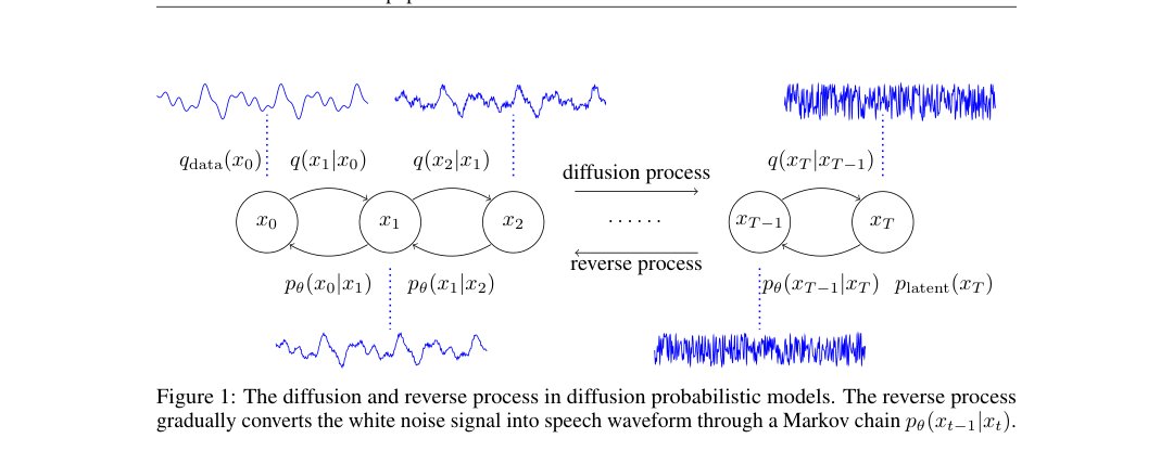
Figure 1: The diffusion and reverse process in diffusion probabilistic models. The reverse process gradually converts the white noise signal into speech waveform through a Markov chain .
图 1:扩散概率模型中的扩散过程与反向过程。反向过程经马尔可夫链 ,把白噪声逐步转成语音波形。
We define as the data distribution on , where is the data dimension. Let for be a sequence of variables with the same dimension, where is the index for diffusion steps. Then, a diffusion model of steps is composed of two processes: the diffusion process, and the reverse process (Sohl-Dickstein et al. 2015). Both of them are illustrated in Figure 1.
令 为 上的数据分布, 为数据维数。对 ,设 为同维变量序列, 为扩散步下标。 步扩散模型由扩散过程与反向过程两部分组成(Sohl-Dickstein et al. 2015),见图 1。
for do
Sample , , and
Take gradient step on according to Eq. (7)
end for
Algorithm 1 Training
for do
Sample , , and
Take gradient step on according to Eq. (7)
end for
算法 1 训练
Sample
for do
Compute and using Eq. (5)
Sample
end for
return
Algorithm 2 Sampling
Sample
for do
Compute and using Eq. (5)
Sample
end for
return
算法 2 采样
The diffusion process is defined by a fixed Markov chain from data to the latent variable :
扩散过程定义为从数据 到隐变量 的固定马尔可夫链:
where each of is fixed to for a small positive constant . The function of is to add small Gaussian noise to the distribution of . The whole process gradually converts data to whitened latents according to a variance schedule . [^2]
其中每个 固定为 , 为小的正常数。 的作用是给 的分布加上小幅高斯噪声。整条过程按方差日程 ,把数据 逐步变成白化隐变量 。[^2]
The reverse process is defined by a Markov chain from to parameterized by :
反向过程定义为由 参数化、从 到 的马尔可夫链:
where is isotropic Gaussian, and the transition probability is parameterized as with shared parameter . Note that both and take two inputs: the diffusion-step , and variable . outputs an -dimensional vector as the mean, and outputs a real number as the standard deviation. The goal of is to eliminate the Gaussian noise (i.e. denoise) added in the diffusion process.
其中 为各向同性高斯,转移概率 参数化为 ,参数 共享。注意 与 都接收两个输入:扩散步 与变量 。 输出 维均值向量, 输出实数标准差。 的目标是消除扩散过程中加入的高斯噪声(即去噪)。
Sampling: Given the reverse process, the generative procedure is to first sample an , and then sample for . The output is the sampled data.
采样:有了反向过程,生成流程是先采样 ,再对 依次采样 。输出 即为采样数据。
Training: The likelihood is intractable to calculate in general. The model is thus trained by maximizing its variational lower bound (ELBO):
训练:似然 一般不可积,因而通过最大化变分下界(ELBO)训练:
Most recently, Ho et al. 2020 showed that under a certain parameterization, the ELBO of the diffusion model can be calculated in closed-form. This accelerates the computation and avoids Monte Carlo estimates, which have high variance. This parameterization is motivated by its connection to denoising score matching with Langevin dynamics (Song & Ermon 2019; Song & Ermon 2020). To introduce this parameterization, we first define some constants based on the variance schedule in the diffusion process as in Ho et al. 2020:
Ho et al. 2020 最近表明:在特定参数化下,扩散模型的 ELBO 可闭式计算。这加速了计算,也避免了方差很大的蒙特卡洛估计。该参数化的动机来自与朗之万动力学下的去噪分数匹配的联系(Song & Ermon 2019;Song & Ermon 2020)。引入参数化前,先按 Ho et al. 2020,依扩散过程方差日程 定义若干常数:
Then, the parameterizations of and are defined by
于是 与 的参数化为
where is a neural network also taking and the diffusion-step as inputs. Note that is fixed to a constant for every step under this parameterization. In the following proposition, we explicitly provide the closed-form expression of the ELBO.
其中 也是以 与扩散步 为输入的神经网络。注意在此参数化下, 对每一步 固定为常数 。下面命题给出 ELBO 的闭式。
Proposition 1.
(Ho et al. 2020)Suppose a series of fixed schedule are given. Let and . Then, under the parameterization in Eq. (5), we have
命题 1。
(Ho et al. 2020)给定固定日程 。令 ,。则在式 (5) 的参数化下,有
for some constants and , where for , and .
其中 与 为常数,(),。
Note that is irrelevant for optimization purpose. The key idea in the proof is to expand the ELBO into a sum of KL divergences between tractable Gaussian distributions, which have a closed-form expression. We refer the readers to look at Section A in the Appendix for the full proof.
注意优化时可忽略 。证明的关键是把 ELBO 展开成一串可处理高斯分布之间的 KL 散度,从而得到闭式。完整证明见附录 A。
In addition, Ho et al. 2020 reported that minimizing the following unweighted variant of the ELBO leads to higher generation quality:
此外,Ho et al. 2020 报告:最小化下列未加权的 ELBO 变体可得到更高生成质量:
where is uniformly taken from . Therefore, we also use this training objective in this paper. We summarize the training and sampling procedures in Algorithm 1 and 2, respectively.
其中 在 上均匀取样。本文亦采用该训练目标。训练与采样流程分别总结于算法 1 与算法 2。
Fast sampling: Given a trained model from Algorithm 1, we noticed that the most effective denoising steps at sampling occur near (see Section IV on demo website). This encourages us to design a fast sampling algorithm with much fewer denoising steps (e.g., 6) than at training (e.g., 200). The key idea is to “collapse” the -step reverse process into a -step process with carefully designed variance schedule. We provide the details in Appendix B.
快速采样:按算法 1 训好模型后,我们观察到采样时最有效的去噪步集中在靠近 处(见演示网站第 IV 节)。这促使我们设计快速采样算法:推理去噪步数 (例如 6)远少于训练时的 (例如 200)。关键是把 步反向过程「折叠」成带精心设计方差日程的 步过程。细节见附录 B。
3 DiffWave Architecture
3 DiffWave 结构
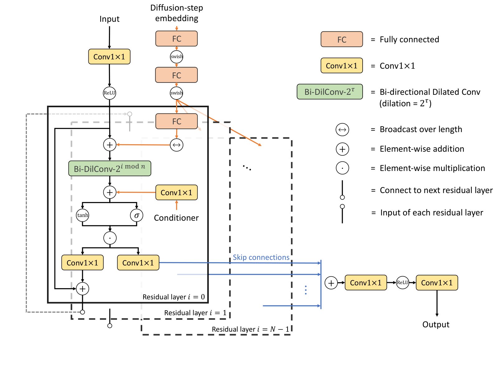
Figure 2: The network architecture of DiffWave in modeling .
图 2:DiffWave 在建模 时的网络结构。
In this section, we present the architecture of DiffWave (see Figure 2 for an illustration). We build the network in Eq. (5) based on a bidirectional dilated convolution architecture that is different from WaveNet (van den Oord et al. 2016), because there is no autoregressive generation constraint. [^3] The similar architecture has been applied for source separation (Rethage et al. 2018; Lluís et al. 2018). The network is non-autoregressive, so generating an audio with length from latents requires rounds of forward propagation, where (e.g., 50) is much smaller than the waveform length . The network is composed of a stack of residual layers with residual channels . These layers are grouped into blocks and each block has layers. We use a bidirectional dilated convolution (Bi-DilConv) with kernel size in each layer. The dilation is doubled at each layer within each block, i.e., . We sum the skip connections from all residual layers as in WaveNet. More details including the tensor shapes are included in Section C in the Appendix.
本节给出 DiffWave 的结构(示意见图 2)。我们基于双向扩张卷积构建式 (5) 中的网络 ;因无自回归生成约束,它与 WaveNet(van den Oord et al. 2016)不同。[^3]类似结构也曾用于源分离(Rethage et al. 2018;Lluís et al. 2018)。网络非自回归,故从隐变量 生成长度为 的音频 只需 轮前向,(例如 50)远小于波形长度 。网络由 个残差层堆叠而成,残差通道数为 ;这些层分成 个块,每块 层。每层使用核大小为 3 的双向扩张卷积(Bi-DilConv);块内扩张按层倍增,即 。与 WaveNet 一样,对各残差层的跳跃连接求和。含张量形状的更多细节见附录 C。
3.1 Diffusion-step Embedding
3.1 扩散步嵌入
It is important to include the diffusion-step as part of the input, as the model needs to output different for different . We use an 128-dimensional encoding vector for each (Vaswani et al. 2017):
把扩散步 纳入输入很重要,因为模型需对每个 输出不同的 。我们对每个 使用 128 维编码向量(Vaswani et al. 2017):
\begin{array}[]{l}\displaystyle t_{\mathrm{embedding}}=\left[\sin\left(10^{\frac{0\times 4}{63}}t\right),\cdots,\sin\left(10^{\frac{63\times 4}{63}}t\right),\right.\left.\cos\left(10^{\frac{0\times 4}{63}}t\right),\cdots,\cos\left(10^{\frac{63\times 4}{63}}t\right)\right]\end{array} \tag{8}
We then apply three fully connected (FC) layers on the encoding, where the first two FCs share parameters among all residual layers. The last residual-layer-specific FC maps the output of the second FC into a -dimensional embedding vector. We next broadcast this embedding vector over length and add it to the input of every residual layer.
再对编码接三层全连接(FC):前两层在所有残差层间共享参数;最后一层为各残差层独有,把第二层 FC 的输出映到 维嵌入向量。随后将该嵌入沿长度维广播,加到每个残差层的输入上。
3.2 Conditional generation
3.2 条件生成
Local conditioner: In speech synthesis, a neural vocoder can synthesize the waveform conditioned on the aligned linguistic features (van den Oord et al. 2016; Arık et al. 2017b), the mel spectrogram from a text-to-spectrogram model (Ping et al. 2018; Shen et al. 2018), or the hidden states within the text-to-wave architecture (Ping et al. 2019; Donahue et al. 2020). In this work, we test DiffWave as a neural vocoder conditioned on mel spectrogram. We first upsample the mel spectrogram to the same length as waveform through transposed 2-D convolutions. After a layer-specific Conv11 mapping its mel-band into channels, the conditioner is added as a bias term for the dilated convolution in each residual layer. The hyperparameters can be found in Section 5.1.
局部条件: 语音合成中,神经声码器可在对齐语言学特征(van den Oord et al. 2016;Arık et al. 2017b)、文本–频谱模型给出的梅尔谱(Ping et al. 2018;Shen et al. 2018),或文本–波形架构内的隐状态(Ping et al. 2019;Donahue et al. 2020)上合成波形。本文把 DiffWave 作为以梅尔谱为条件的神经声码器来测试。先用转置二维卷积把梅尔谱上采样到与波形同长;再经层专属的 Conv11 把梅尔频带映到 通道,作为偏置加到各残差层的扩张卷积上。超参见第 5.1 节。
Global conditioner: In many generative tasks, the conditional information is given by global discrete labels (e.g., speaker IDs or word IDs). We use shared embeddings with dimension in all experiments. In each residual layer, we apply a layer-specific Conv11 to map to channels, and add the embedding as a bias term after the dilated convolution in each residual layer.
全局条件: 许多生成任务的条件是全局离散标签(如说话人 ID 或词 ID)。全部实验使用维度 的共享嵌入。每个残差层用层专属 Conv11 把 映到 通道,作为偏置加在扩张卷积之后。
3.3 Unconditional generation
3.3 无条件生成
In unconditional generation task, the model needs to generate consistent utterances without conditional information. It is important for the output units of the network to have a receptive field size (denoted as ) larger than the length of the utterance. Indeed, we need , thus the left and right-most output units have receptive fields covering the whole -dimensional inputs as illustrated in Figure 4 in Appendix C. This posts a challenge for architecture design even with the dilated convolutions.
无条件生成要求模型在没有条件信息时仍能产出前后一致的话语。网络输出单元的感受野(记为 )必须大于话语长度 。实际上需要 ,使最左、最右输出单元的感受野都能覆盖整段 维输入,见附录 C 图 4。即便使用扩张卷积,这对结构设计仍是挑战。
For a stack of dilated convolution layers, the receptive field size of the output is up to: , where is the kernel size and is the dilation at -th residual layer. For example, 30-layer dilated convolution has a receptive field size , with and dilation cycle . This only amounts to 0.38s of 16kHz audio. We can further increase the number of layers and the size of dilation cycles; however, we found degraded quality with deeper layers and larger dilation cycles. This is particularly true for WaveNet. In fact, previous study (Shen et al. 2018) suggests that even a moderate large receptive field size (e.g., 6139) is not effectively used in WaveNet and it tends to focus on much shorter context (e.g., 500). DiffWave has an advantage in enlarging the receptive fields of output : by iterating from to in the reverse process, the receptive field size can be increased up to , which makes DiffWave suitable for unconditional generation.
对一叠扩张卷积层,输出感受野至多为 ,其中 为核大小, 为第 个残差层的扩张。例如 30 层扩张卷积、核 、扩张周期 时,,对 16kHz 音频仅约 0.38 秒。还可加层、加大扩张周期,但更深、更大扩张往往反而掉质量,WaveNet 尤其如此。先前研究(Shen et al. 2018)也提示:即便感受野中等偏大(如 6139),WaveNet 也未必用满,往往只关注短得多的上下文(如 500)。DiffWave 在扩大输出 感受野上有优势:反向过程从 迭代到 ,感受野可增至约 ,因而更适合无条件生成。
4 Related Work
4 相关工作
In the past years, many neural text-to-speech (TTS) systems have been introduced. An incomplete list includes WaveNet (van den Oord et al. 2016), Deep Voice 1 & 2 & 3 (Arık et al. 2017a; Arık et al. 2017b; Ping et al. 2018), Tacotron 1 & 2 (Wang et al. 2017; Shen et al. 2018), Char2Wav (Sotelo et al. 2017), VoiceLoop (Taigman et al. 2018), Parallel WaveNet (van den Oord et al. 2018), WaveRNN (Kalchbrenner et al. 2018), ClariNet (Ping et al. 2019), ParaNet (Peng et al. 2020), FastSpeech (Ren et al. 2019), GAN-TTS (Bińkowski et al. 2020), and Flowtron (Valle et al. 2020). These systems first generate intermediate representations (e.g., aligned linguistic features, mel spectrogram, or hidden representations) conditioned on text, then use a neural vocoder to synthesize the raw waveform.
过去数年出现了许多神经文本转语音(TTS)系统。不完全列举包括 WaveNet(van den Oord et al. 2016)、Deep Voice 1 & 2 & 3(Arık et al. 2017a;Arık et al. 2017b;Ping et al. 2018)、Tacotron 1 & 2(Wang et al. 2017;Shen et al. 2018)、Char2Wav(Sotelo et al. 2017)、VoiceLoop(Taigman et al. 2018)、Parallel WaveNet(van den Oord et al. 2018)、WaveRNN(Kalchbrenner et al. 2018)、ClariNet(Ping et al. 2019)、ParaNet(Peng et al. 2020)、FastSpeech(Ren et al. 2019)、GAN-TTS(Bińkowski et al. 2020)以及 Flowtron(Valle et al. 2020)。这些系统通常先按文本生成中间表示(如对齐语言学特征、梅尔谱或隐表示),再用神经声码器合成原始波形。
Neural vocoder plays the most important role in the recent success of speech synthesis. Autoregressive models like WaveNet and WaveRNN can generate high-fidelity speech, but in a sequential way of generation. Parallel WaveNet and ClariNet distill parallel flow-based models from WaveNet, thus can synthesize waveform in parallel. In contrast, WaveFlow (Ping et al. 2020), WaveGlow (Prenger et al. 2019) and FloWaveNet (Kim et al. 2019) are trained by maximizing likelihood. There are other waveform models, such as VAE-based models (Peng et al. 2020), GAN-based models (Kumar et al. 2019; Yamamoto et al. 2020; Bińkowski et al. 2020), and neural signal processing models (Wang et al. 2019; Engel et al. 2020; Ai & Ling 2020). In contrast to likelihood-based models, they often require auxiliary training losses to improve the audio fidelity. The proposed DiffWave is another promising neural vocoder synthesizing the best quality of speech with a single objective function.
神经声码器是近期语音合成成功的关键。WaveNet、WaveRNN 等自回归模型可生成高保真语音,但是串行生成。Parallel WaveNet 与 ClariNet 从 WaveNet 蒸馏出可并行的流模型,因而能并行合成波形。相对地,WaveFlow(Ping et al. 2020)、WaveGlow(Prenger et al. 2019)与 FloWaveNet(Kim et al. 2019)以最大化似然训练。另有基于 VAE 的模型(Peng et al. 2020)、基于 GAN 的模型(Kumar et al. 2019;Yamamoto et al. 2020;Bińkowski et al. 2020)以及神经信号处理模型(Wang et al. 2019;Engel et al. 2020;Ai & Ling 2020)。相对基于似然的模型,它们常需辅助训练损失来抬高音质。本文提出的 DiffWave 是另一类有潜力的神经声码器:用单一目标函数即可合成当时最高水准的语音质量。
Unconditional generation of audio in the time domain is a challenging task in general. Likelihood-based models are forced to learn all possible variations within the dataset without any conditional information, which can be quite difficult with limited model capacity. In practice, these models produce made-up word-like sounds or inferior samples (van den Oord et al. 2016; Donahue et al. 2019). VQ-VAE (van den Oord et al. 2017) circumvents this issue by compressing the waveform into compact latent code, and training an autoregressive model in latent domain. GAN-based models are believed to be suitable for unconditional generation (Donahue et al. 2019, e.g.,) due to the “mode seeking” behaviour and success in image domain (Brock et al. 2018). Note that unconditional generation of audio in the frequency domain is considered easier, as the spectrogram is much shorter (e.g., 200) than waveform (Vasquez & Lewis 2019; Engel et al. 2019; Palkama et al. 2020).
时域音频的无条件生成整体上很难。基于似然的模型被迫在无任何条件信息时学尽数据集内全部变化,模型容量有限时相当困难。实践中这些模型常产出虚构词样声音或较差样本(van den Oord et al. 2016;Donahue et al. 2019)。VQ-VAE(van den Oord et al. 2017)把波形压成紧凑隐码,再在隐空间训自回归模型,从而绕开难题。基于 GAN 的模型因「寻模」行为以及在图像域的成功(Brock et al. 2018),被认为适合无条件生成(例如 Donahue et al. 2019)。需注意频域无条件生成相对更容易:频谱比波形短得多(例如短 )(Vasquez & Lewis 2019;Engel et al. 2019;Palkama et al. 2020)。
In this work, we demonstrate the superior performance of DiffWave in unconditional generation of waveform. In contrast to the exact-likelihood models, DiffWave maximizes a variational lower bound of the likelihood, which can focus on the major variations within the data and alleviate the requirements for model capacity. In contrast to GAN or VAE-based models (Donahue et al. 2019; Peng et al. 2020), it is much easier to train without mode collapse, posterior collapse, or training instability stemming from the joint training of two networks. There is a concurrent work (Chen et al. 2020) that uses diffusion probabilistic models for waveform generation. In contrast to DiffWave, it uses a neural architecture similar to GAN-TTS and focuses on the neural vocoding task only. Our DiffWave vocoder has much fewer parameters than WaveGrad – 2.64M vs. 15M for Base models and 6.91M vs. 23M for Large models. The small memory footprint is preferred in production TTS systems, especially for on-device deployment. In addition, DiffWave requires a smaller batch size (16 vs. 256) and fewer computational resources for training.
本文展示 DiffWave 在波形无条件生成上的出色表现。相对精确似然模型,DiffWave 最大化似然的变分下界,可聚焦数据中的主要变化,从而减轻对模型容量的要求。相对基于 GAN 或 VAE 的模型(Donahue et al. 2019;Peng et al. 2020),它无需双网络联合训练带来的模式坍塌、后验坍塌或不稳定,因而更容易训。同期工作(Chen et al. 2020)也把扩散概率模型用于波形生成;相对 DiffWave,它采用类似 GAN-TTS 的神经结构,且只聚焦神经声码。我们的 DiffWave 声码器参数远少于 WaveGrad——Base 为 2.64M 对 15M,Large 为 6.91M 对 23M。生产 TTS、尤其端侧部署更偏好小体积。此外 DiffWave 训练所需批大小更小(16 对 256),算力需求也更低。
5 Experiments
5 实验
We evaluate DiffWave on neural vocoding, unconditional and class-conditional generation tasks.
我们在神经声码、无条件生成与类别条件生成任务上评测 DiffWave。
5.1 Neural vocoding
5.1 神经声码
Data: We use the LJ speech dataset (Ito 2017) that contains 24 hours of audio recorded in home environment with a sampling rate of 22.05 kHz. It contains 13,100 utterances from a female speaker.
数据: 使用 LJ Speech 数据集(Ito 2017):约 24 小时、采样率 22.05 kHz、家庭环境录制的音频,含一名女说话人的 13,100 条话语。
Models: We compare DiffWave with several state-of-the-art neural vocoders, including WaveNet, ClariNet, WaveGlow and WaveFlow. Details of baseline models can be found in the original papers. Their hyperparameters can be found in Table 1. Our DiffWave models have 30 residual layers, kernel size 3, and dilation cycle . We compare DiffWave models with different number of diffusion steps and residual channels . We use linear spaced schedule for for DiffWave with , and for DiffWave with . The reason to increase for smaller is to make close to . In addition, we compare the fast sampling algorithm with smaller (see Appendix B), denoted as DiffWave (Fast), with the regular sampling (Algorithm 2). Both of them use the same trained models.
模型: 将 DiffWave 与 WaveNet、ClariNet、WaveGlow、WaveFlow 等当时前沿神经声码器对比。基线细节见原文,超参见表 1。我们的 DiffWave 为 30 个残差层、核大小 3、扩张周期 。比较不同扩散步数 与残差通道 。 时 在 上线性间隔; 时在 上线性间隔。对较小 增大 ,是为使 更接近 。另将快速采样(更小 ,见附录 B)记为 DiffWave (Fast),与常规采样(算法 2)对比;二者共用同一训好模型。
Conditioner: We use the 80-band mel spectrogram of the original audio as the conditioner to test these neural vocoders as in previous work (Ping et al. 2019; Prenger et al. 2019; Kim et al. 2019). We set FFT size to 1024, hop size to 256, and window size to 1024. We upsample the mel spectrogram 256 times by applying two layers of transposed 2-D convolution (in time and frequency) interleaved with leaky ReLU (). For each layer, the upsamling stride in time is 16 and 2-D filter sizes are . After upsampling, we use a layer-specific Conv11 to map the 80 mel bands into residual channels, then add the conditioner as a bias term for the dilated convolution before the gated-tanh nonlinearities in each residual layer.
条件: 与既往工作相同(Ping et al. 2019;Prenger et al. 2019;Kim et al. 2019),用原始音频的 80 带梅尔谱作条件。FFT 大小 1024,hop 256,窗长 1024。用两层转置二维卷积(时间与频率)交错 leaky ReLU(),把梅尔谱上采样 256 倍;每层时间上采样步长为 16,二维滤波大小 。上采样后,用层专属 Conv11 把 80 个梅尔带映到 残差通道,再作为偏置加到各残差层门控 tanh 非线性之前的扩张卷积上。
Training: We train DiffWave on 8 Nvidia 2080Ti GPUs using random short audio clips of 16,000 samples from each utterance. We use Adam optimizer (Kingma & Ba 2015) with a batch size of 16 and learning rate . We train all DiffWave models for 1M steps. For other models, we follow the training setups as in the original papers.
训练: 在 8 块 Nvidia 2080Ti 上训练 DiffWave,每条话语随机截取 16,000 采样点的短片段。Adam 优化器(Kingma & Ba 2015),批大小 16,学习率 。全部 DiffWave 训 100 万步。其他模型按原文设定训练。
| Model width 1pt | layers | res. channels | #param() | MOS() | ||
|---|---|---|---|---|---|---|
| WaveNet width 1pt | — | — | 30 | 128 | 4.57M | |
| ClariNet width 1pt | — | — | 60 | 64 | 2.17M | |
| WaveGlow width 1pt | — | — | 96 | 256 | 87.88M | |
| WaveFlow width 1pt | — | — | 64 | 64 | 5.91M | |
| WaveFlow width 1pt | — | — | 64 | 128 | 22.25M | |
| width 1pt | 20 | 20 | 30 | 64 | 2.64M | |
| width 1pt | 40 | 40 | 30 | 64 | 2.64M | |
| width 1pt | 50 | 50 | 30 | 64 | 2.64M | |
| width 1pt | 200 | 200 | 30 | 128 | 6.91M | |
| width 1pt | 50 | 6 | 30 | 64 | 2.64M | |
| width 1pt | 200 | 6 | 30 | 128 | 6.91M | |
| Ground-truth width 1pt | — | — | — | — | — |
Table 1: The model hyperparameters, model footprint, and 5-scale Mean Opinion Score (MOS) with 95% confidence intervals for WaveNet, ClariNet, WaveFlow, WaveGlow and the proposed DiffWave on the neural vocoding task. means the number is the higher the better, and means the number is the lower the better.
| 模型 | 层数 | 残差通道 | 参数量() | MOS() | ||
|---|---|---|---|---|---|---|
| WaveNet | — | — | 30 | 128 | 4.57M | |
| ClariNet | — | — | 60 | 64 | 2.17M | |
| WaveGlow | — | — | 96 | 256 | 87.88M | |
| WaveFlow | — | — | 64 | 64 | 5.91M | |
| WaveFlow | — | — | 64 | 128 | 22.25M | |
| 20 | 20 | 30 | 64 | 2.64M | ||
| 40 | 40 | 30 | 64 | 2.64M | ||
| 50 | 50 | 30 | 64 | 2.64M | ||
| 200 | 200 | 30 | 128 | 6.91M | ||
| 50 | 6 | 30 | 64 | 2.64M | ||
| 200 | 6 | 30 | 128 | 6.91M | ||
| 真值 | — | — | — | — | — |
表 1:WaveNet、ClariNet、WaveFlow、WaveGlow 与本文 DiffWave 在神经声码任务上的超参、模型体积与 5 分制平均意见分(MOS,含 95% 置信区间)。 表示越大越好, 表示越小越好。
Results: We use the crowdMOS tookit (Ribeiro et al. 2011) for speech quality evaluation, where the test utterances from all models were presented to Mechanical Turk workers. We report the 5-scale Mean Opinion Scores (MOS), and model footprints in Table 1 [^4]. Our model with residual channels 128 matches the strong WaveNet vocoder in terms of speech quality (MOS: 4.44 vs. 4.43). The with residual channels 64 also generates high quality speech (e.g., MOS: 4.35) even with small number of diffusion steps (e.g., or ). For synthesis speed, () in FP32 generates audio faster than real-time, and () in FP32 is faster than real-time on a Nvidia V100 GPU without engineering optimization. Meanwhile, (Fast) and (Fast) can be and faster than real-time respectively and still obtain good audio fidelity. In contrast, a WaveNet implementation can be slower than real-time at synthesis without engineered kernels. DiffWave is still slower than the state-of-the-art flow-based models (e.g., a 5.91M WaveFlow is faster than real-time in FP16), but has smaller footprint and slightly better quality. Because DiffWave does not impose any architectural constraints as in flow-based models, we expect further speed-up by optimizing the architecture and inference mechanism in the future.
结果: 用 crowdMOS 工具包(Ribeiro et al. 2011)做语音质量评测,把各模型测试话语呈现给 Mechanical Turk 工人。5 分制 MOS 与模型体积见表 1。[^4] 残差通道 128 的 与强 WaveNet 声码器语音质量相当(MOS:4.44 对 4.43)。残差通道 64 的 即便扩散步较少(如 或 )也能生成高质量语音(例如 MOS:4.35)。合成速度上,FP32 的 ()在无工程优化的 Nvidia V100 上比实时快 , 时快 。同时 (Fast)与 (Fast)可分别比实时快 与 ,仍保持较好保真度。相对地,未经专门内核优化的 WaveNet 实现合成可比实时慢 。DiffWave 仍慢于当时最先进的流模型(例如 5.91M 的 WaveFlow 在 FP16 下可比实时快 ),但体积更小、质量略优。因 DiffWave 不像流模型那样施加结构约束,我们预期未来通过优化结构与推理机制还能再加速。
5.2 Unconditional generation
5.2 无条件生成
In this section, we apply DiffWave to an unconditional generation task based on raw waveform only.
本节把 DiffWave 用到仅依赖原始波形的无条件生成任务。
Data: We use the Speech Commands dataset (Warden 2018), which contains many spoken words by thousands of speakers under various recording conditions including some very noisy environment. We select the subset that contains spoken digits (09), which we call the SC09 dataset. The SC09 dataset contains 31,158 training utterances (8.7 hours in total) by 2,032 speakers, where each audio has length equal to one second under sampling rate 16kHz. Therefore, the data dimension is 16,000. Note that the SC09 dataset exhibits various variations (e.g., contents, speakers, speech rate, recording conditions); the generative models need to model them without any conditional information.
数据: 使用 Speech Commands 数据集(Warden 2018),含数千说话人在多种录制条件(含很嘈杂环境)下的大量口语词。我们选取口语数字(0~9)子集,称为 SC09。SC09 含 31,158 条训练话语(合计约 8.7 小时)、2,032 名说话人;每条音频在 16kHz 采样率下长度为一秒,故数据维数 。该集变化很大(内容、说话人、语速、录制条件等),生成模型需在无任何条件信息时建模这些变化。
Models: We compare DiffWave with WaveNet and WaveGAN. We also tried to remove the mel conditioner in a state-of-the-art GAN-based neural vocoder (Yamamoto et al. 2020), but found it could not generate intelligible speech in this unconditional task. We use 30 layer-WaveNet models with residual channels 128 (denoted as WaveNet-128) and 256 (denoted as WaveNet-256), respectively. We tried to increase the size of the dilation cycle and the number of layers, but these modifications lead to worse quality. In particular, a large dilation cycle (e.g., up to 2048) leads to unstable training. For WaveGAN, we use their pretrained model on Google Colab. We use a 36-layer DiffWave model with kernel size 3 and dilation cycle . We set the number of diffusion steps and residual channels . We use linear spaced schedule for .
模型: 将 DiffWave 与 WaveNet、WaveGAN 对比。也曾去掉当时前沿基于 GAN 的神经声码器(Yamamoto et al. 2020)中的梅尔条件,但发现其在无条件任务上无法生成可懂语音。WaveNet 用 30 层、残差通道 128(WaveNet-128)与 256(WaveNet-256)两档;加大扩张周期与层数反而更差,尤其很大扩张周期(如到 2048)会导致训练不稳。WaveGAN 使用 Google Colab 上的预训练模型。DiffWave 用 36 层、核大小 3、扩张周期 ;扩散步 ,残差通道 ; 在 上线性间隔。
Training: We train WaveNet and DiffWave on 8 Nvidia 2080Ti GPUs using full utterances. We use Adam optimizer with a batch size of 16. For WaveNet, we set the initial learning rate as and halve the learning rate every 200K iterations. For DiffWave, we fix the learning rate to . We train WaveNet and DiffWave for 1M steps.
训练: 在 8 块 Nvidia 2080Ti 上用完整话语训练 WaveNet 与 DiffWave。Adam,批大小 16。WaveNet 初始学习率 ,每 20 万迭代减半;DiffWave 固定学习率 。二者均训 100 万步。
Evaluation: For human evaluation, we report the 5-scale MOS for speech quality similar to Section 5.1. To automatically evaluate the quality of generated audio samples, we train a ResNeXT classifier (Xie et al. 2017) on the SC09 dataset according to an open repository (Xu & Tuguldur 2017). The classifier achieves accuracy on the trainset and accuracy on the testset. We use the following evaluation metrics based on the 1024-dimensional feature vector and the 10-dimensional logits from the ResNeXT classifier (see Section D in the Appendix for the detailed definitions):
评测: 听感方面,与第 5.1 节类似报告 5 分制 MOS。自动评测方面,按开源仓库(Xu & Tuguldur 2017)在 SC09 上训练 ResNeXT 分类器(Xie et al. 2017);该分类器训练集准确率 、测试集 。基于其 1024 维特征向量与 10 维 logits,使用下列指标(定义见附录 D):
- • Fréchet Inception Distance (FID) (Heusel et al. 2017) measures both quality and diversity of generated samples, and favors generators that match moments in the feature space.
- • Fréchet Inception Distance(FID)(Heusel et al. 2017)同时衡量生成样本的质量与多样性,偏好在特征空间匹配矩的生成器。
- • Inception Score (IS) (Salimans et al. 2016) measures both quality and diversity of generated samples, and favors generated samples that can be clearly determined by the classifier.
- • Inception Score(IS)(Salimans et al. 2016)同时衡量质量与多样性,偏好能被分类器清晰判定的生成样本。
- • Modified Inception Score (mIS) (Gurumurthy et al. 2017) measures the within-class diversity of samples in addition to IS.
- • Modified Inception Score(mIS)(Gurumurthy et al. 2017)在 IS 之外再衡量类内多样性。
- • AM Score (Zhou et al. 2017) takes into consideration the marginal label distribution of training data compared to IS.
- • AM Score(Zhou et al. 2017)相对 IS 额外考虑训练数据的边缘标签分布。
- • Number of Statistically-Different Bins (NDB) (Richardson & Weiss 2018) measures diversity of generated samples.
- • Number of Statistically-Different Bins(NDB)(Richardson & Weiss 2018)衡量生成样本的多样性。
Results: We randomly generate 1,000 audio samples from each model for evaluation. We report results in Table 2. Our DiffWave model outperforms baseline models under all metrics, including both automatic and human evaluation. Notably, the quality of audio samples generated by DiffWave is much higher than WaveNet and WaveGAN baselines (MOS: 3.39 vs. 1.43 and 2.03). Note that the quality of ground-truth audio exhibits large variations. The automatic evaluation metrics also indicate that DiffWave is better at quality, diversity, and matching marginal label distribution of training data.
结果: 每个模型随机生成 1,000 条音频评测,结果见表 2。DiffWave 在全部指标(含自动与听感)上优于基线。尤为突出的是音质远高于 WaveNet 与 WaveGAN(MOS:3.39 对 1.43 与 2.03)。需注意真值音频质量本身变化也很大。自动指标同样表明 DiffWave 在质量、多样性以及匹配训练数据边缘标签分布上更好。
| Model width 1pt | FID() | IS() | mIS() | AM() | NDB() | MOS() |
|---|---|---|---|---|---|---|
| WaveNet-128 width 1pt | 3.279 | 2.54 | 7.6 | 1.368 | 0.86 | |
| WaveNet-256 width 1pt | 2.947 | 2.84 | 10.0 | 1.260 | 0.86 | |
| WaveGAN width 1pt | 1.349 | 4.53 | 36.6 | 0.796 | 0.78 | |
| DiffWave width 1pt | 1.287 | 5.30 | 59.4 | 0.636 | 0.74 | |
| Trainset width 1pt | 0.000 | 8.48 | 281.4 | 0.164 | 0.00 | — |
| Testset width 1pt | 0.011 | 8.47 | 275.2 | 0.166 | 0.10 |
Table 2: The automatic evaluation metrics (FID, IS, mIS, AM, and NDB), and 5-scale MOS with 95% confidence intervals for WaveNet, WaveGAN, and DiffWave on the unconditional generation task. means the number is the higher the better, and means the number is the lower the better.
| 模型 | FID() | IS() | mIS() | AM() | NDB() | MOS() |
|---|---|---|---|---|---|---|
| WaveNet-128 | 3.279 | 2.54 | 7.6 | 1.368 | 0.86 | |
| WaveNet-256 | 2.947 | 2.84 | 10.0 | 1.260 | 0.86 | |
| WaveGAN | 1.349 | 4.53 | 36.6 | 0.796 | 0.78 | |
| DiffWave | 1.287 | 5.30 | 59.4 | 0.636 | 0.74 | |
| 训练集 | 0.000 | 8.48 | 281.4 | 0.164 | 0.00 | — |
| 测试集 | 0.011 | 8.47 | 275.2 | 0.166 | 0.10 |
表 2:WaveNet、WaveGAN 与 DiffWave 在无条件生成任务上的自动指标(FID、IS、mIS、AM、NDB)以及含 95% 置信区间的 5 分制 MOS。 越大越好, 越小越好。
| Model width 1pt | Accuracy() | FID-class() | IS() | mIS() | MOS() |
|---|---|---|---|---|---|
| WaveNet-128 width 1pt | 56.20% | 7.8762.469 | 3.29 | 15.8 | |
| WaveNet-256 width 1pt | 60.70% | 6.9542.114 | 3.46 | 18.9 | |
| DiffWave width 1pt | 91.20% | 1.1130.569 | 6.63 | 117.4 | |
| DiffWave (deep & thin) width 1pt | 94.00% | **0.932**0.450 | 6.92 | 133.8 | |
| Trainset width 1pt | 99.06% | 0.0000.000 | 8.48 | 281.4 | — |
| Testset width 1pt | 98.76% | 0.0440.016 | 8.47 | 275.2 |
Table 3: The automatic evaluation metrics (Accuracy, FID-class, IS, mIS), and 5-scale MOS with 95% confidence intervals for WaveNet and DiffWave on the class-conditional generation task.
| 模型 | 准确率() | FID-class() | IS() | mIS() | MOS() |
|---|---|---|---|---|---|
| WaveNet-128 | 56.20% | 7.8762.469 | 3.29 | 15.8 | |
| WaveNet-256 | 60.70% | 6.9542.114 | 3.46 | 18.9 | |
| DiffWave | 91.20% | 1.1130.569 | 6.63 | 117.4 | |
| DiffWave(深而窄) | 94.00% | **0.932**0.450 | 6.92 | 133.8 | |
| 训练集 | 99.06% | 0.0000.000 | 8.48 | 281.4 | — |
| 测试集 | 98.76% | 0.0440.016 | 8.47 | 275.2 |
表 3:WaveNet 与 DiffWave 在类别条件生成任务上的自动指标(准确率、FID-class、IS、mIS)以及含 95% 置信区间的 5 分制 MOS。
5.3 Class-conditional generation
5.3 类别条件生成
In this section, we provide the digit labels as the conditioner in DiffWave and compare our model to WaveNet. We omit the comparison with conditional WaveGAN due to its noisy output audio (Lee et al. 2018). For both DiffWave and WaveNet, the label conditioner is added to the model according to Section 3.2. We use the same dataset, model hyperparameters, and training settings as in Section 5.2.
本节把数字标签作为 DiffWave 的条件,并与 WaveNet 对比。因条件 WaveGAN 输出噪声很大(Lee et al. 2018),省略与其对比。DiffWave 与 WaveNet 均按第 3.2 节加入标签条件。数据、超参与训练设定与第 5.2 节相同。
Evaluation: We use slightly different automatic evaluation methods in this section because audio samples are generated according to pre-specified discrete labels. The AM score and NDB are removed because they are less meaningful when the prior label distribution of generated data is specified. We keep IS and mIS because IS favors sharp, clear samples and mIS measures within-class diversity. We modify FID to FID-class: for each digit from 0 to 9, we compute FID between the generated audio samples that are pre-specified as this digit and training utterances with the same digit labels, and report the mean and standard deviation of these ten FID scores. We also report classification accuracy based on the ResNeXT classifier used in Section 5.2.
评测: 因样本按预先指定的离散标签生成,自动评测略有调整:去掉对给定先验标签分布意义不大的 AM 与 NDB;保留偏好清晰样本的 IS,以及衡量类内多样性的 mIS。将 FID 改为 FID-class:对数字 0 到 9,分别计算预先指定为该数字的生成样本与同标签训练话语之间的 FID,再报告这十个分数的均值与标准差。另报告第 5.2 节所用 ResNeXT 分类器的分类准确率。
Results: We randomly generate 100 audio samples for each digit (0 to 9) from all models for evaluation. We report results in Table 3. Our DiffWave model significantly outperforms WaveNet on all evaluation metrics. It produces superior quality than WaveNet (MOS: 3.50 vs. 1.58), and greatly decreases the gap to ground-truth (the gap between DiffWave and ground-truth is 10% of the gap between WaveNet and ground-truth). The automatic evaluation metrics indicate that DiffWave is much better at speech clarity ( accuracy) and within-class diversity (its mIS is higher than WaveNet). We additionally found a deep and thin version of DiffWave with residual channels and 48 residual layers can achieve slightly better accuracy but lower audio quality. One may also compare quality of generated audio samples between conditional and unconditional generation based on IS, mIS, and MOS. For both WaveNet and DiffWave, IS increases by 20%, mIS almost doubles, and MOS increases by . These results indicate that the digit labels reduces the difficulty of the generative task and helps improving the generation quality of WaveNet and DiffWave.
结果: 每个模型对每个数字(0 到 9)随机生成 100 条音频,结果见表 3。DiffWave 在全部指标上显著优于 WaveNet:音质更高(MOS:3.50 对 1.58),相对真值的差距约为 WaveNet–真值差距的 10%。自动指标显示语音清晰度更高(准确率 ),类内多样性也大得多(mIS 约为 WaveNet 的 )。另外发现残差通道 、48 层的深而窄 DiffWave 准确率略高,但音质略低。也可凭 IS、mIS 与 MOS 比较条件与无条件生成质量:对 WaveNet 与 DiffWave,IS 均提升 ,mIS 几乎翻倍,MOS 至少升 。说明数字标签降低了生成难度,并帮助提升 WaveNet 与 DiffWave 的生成质量。
5.4 Additional results
5.4 补充结果
Zero-shot speech denoising: The unconditional DiffWave model can readily perform speech denoising. The SC09 dataset provides six types of noises for data augmentation in recognition tasks: white noise, pink noise, running tap, exercise bike, dude miaowing, and doing the dishes. These noises are not used during the training phase of our unconditional DiffWave in Section 5.2. We add 10% of each type of noise to test data, feed these noisy utterances into the reverse process at , and then obtain the outputs ’s. The audio samples are in Section V on the demo website. Note that our model is not trained on a denoising task and has zero knowledge about any noise type other than the white noise added in diffusion process. It indicates DiffWave learns a good prior of raw audio.
零样本语音去噪: 无条件 DiffWave 可直接用于语音去噪。SC09 为识别数据增广提供了六类噪声:白噪声、粉红噪声、流水、健身车、猫叫与洗碗;这些噪声未用于第 5.2 节无条件 DiffWave 的训练。我们向测试数据加入 10% 各类噪声,在 把带噪话语送入反向过程,得到输出 。样本见演示网站第 V 节。模型并未在去噪任务上训练,除扩散过程中的白噪声外对其余噪声类型零知识,这表明 DiffWave 学到了较好的原始音频先验。
Interpolation in latent space: We can do interpolation with the digit conditioned DiffWave model in Section 5.3 on the SC09 dataset. The interpolation of voices between two speakers is done in the latent space at . We first sample and for the two speakers. We then do linear interpolation between and : for . Finally, we sample . The audio samples are in Section VI on the demo website.
隐空间插值: 可用第 5.3 节数字条件 DiffWave 在 SC09 上做插值。说话人 之间语音 的插值在 的隐空间进行:先采样 与 ,再线性插值 (),最后采样 。样本见演示网站第 VI 节。
6 Conclusion
6 结论
In this paper, we present DiffWave, a versatile generative model for raw waveform. In the neural vocoding task, it readily models the fine details of waveform conditioned on mel spectrogram and matches the strong autoregressive neural vocoder in terms of speech quality. In unconditional and class-conditional generation tasks, it properly captures the large variations within the data and produces realistic voices and consistent word-level pronunciations. To the best of our knowledge, DiffWave is the first waveform model that exhibits such versatility. DiffWave raises a number of open problems and provides broad opportunities for future research. For example, it would be meaningful to push the model to generate longer utterances, as DiffWave potentially has very large receptive fields. Second, optimizing the inference speed would be beneficial for applying the model in production TTS, because DiffWave is still slower than flow-based models. We found the most effective denoising steps in the reverse process occur near , which suggests an even smaller is possible in DiffWave. In addition, the model parameters are shared across the reverse process, so the persistent kernels that stash the parameters on-chip would largely speed-up inference on GPUs (Diamos et al. 2016).
本文提出面向原始波形的通用生成模型 DiffWave。在神经声码任务上,它能在梅尔谱条件下刻画波形细部,语音质量与强自回归神经声码器相当;在无条件与类别条件生成上,它能恰当捕获数据中的大幅变化,产出逼真嗓音与连贯的词级发音。据我们所知,DiffWave 是首个展现此类通用性的波形模型。它也留下若干开放问题与广阔后续空间:例如推动模型生成更长话语——DiffWave 潜在感受野可以很大;再如优化推理速度以利于生产 TTS——DiffWave 仍慢于流模型。我们发现反向过程中最有效的去噪步靠近 ,暗示 DiffWave 还可能用更小的 。此外模型参数 在反向过程中共享,若用把参数常驻片上的持久内核,有望在 GPU 上大幅加速推理(Diamos et al. 2016)。
References
参考文献
Ai & Ling (2020) Yang Ai and Zhen-Hua Ling. A neural vocoder with hierarchical generation of amplitude and phase spectra for statistical parametric speech synthesis. IEEE/ACM Transactions on Audio, Speech, and Language Processing , 28:839–851, 2020.
Arık et al. (2017a) Sercan Ö. Arık, Mike Chrzanowski, Adam Coates, Gregory Diamos, Andrew Gibiansky, Yongguo Kang, Xian Li, John Miller, Jonathan Raiman, Shubho Sengupta, and Mohammad Shoeybi. Deep Voice: Real-time neural text-to-speech. In ICML , 2017a.
Arık et al. (2017b) Sercan Ö. Arık, Gregory Diamos, Andrew Gibiansky, John Miller, Kainan Peng, Wei Ping, Jonathan Raiman, and Yanqi Zhou. Deep Voice 2: Multi-speaker neural text-to-speech. In NIPS , 2017b.
Bińkowski et al. (2020) Mikołaj Bińkowski, Jeff Donahue, Sander Dieleman, Aidan Clark, Erich Elsen, Norman Casagrande, Luis C Cobo, and Karen Simonyan. High fidelity speech synthesis with adversarial networks. In ICLR , 2020.
Brock et al. (2018) Andrew Brock, Jeff Donahue, and Karen Simonyan. Large scale GAN training for high fidelity natural image synthesis. arXiv preprint arXiv:1809.11096 , 2018.
Chen et al. (2020) Nanxin Chen, Yu Zhang, Heiga Zen, Ron J Weiss, Mohammad Norouzi, and William Chan. WaveGrad: Estimating gradients for waveform generation. arXiv preprint arXiv:2009.00713 , 2020.
Diamos et al. (2016) Greg Diamos, Shubho Sengupta, Bryan Catanzaro, Mike Chrzanowski, Adam Coates, Erich Elsen, Jesse Engel, Awni Hannun, and Sanjeev Satheesh. Persistent rnns: Stashing recurrent weights on-chip. In International Conference on Machine Learning , pp. 2024–2033, 2016.
Donahue et al. (2019) Chris Donahue, Julian McAuley, and Miller Puckette. Adversarial audio synthesis. In ICLR , 2019.
Donahue et al. (2020) Jeff Donahue, Sander Dieleman, Mikołaj Bińkowski, Erich Elsen, and Karen Simonyan. End-to-end adversarial text-to-speech. arXiv preprint arXiv:2006.03575 , 2020.
Engel et al. (2019) Jesse Engel, Kumar Krishna Agrawal, Shuo Chen, Ishaan Gulrajani, Chris Donahue, and Adam Roberts. Gansynth: Adversarial neural audio synthesis. In ICLR , 2019.
Engel et al. (2020) Jesse Engel, Lamtharn Hantrakul, Chenjie Gu, and Adam Roberts. Ddsp: Differentiable digital signal processing. arXiv preprint arXiv:2001.04643 , 2020.
Goodfellow et al. (2014) Ian Goodfellow, Jean Pouget-Abadie, Mehdi Mirza, Bing Xu, David Warde-Farley, Sherjil Ozair, Aaron Courville, and Yoshua Bengio. Generative adversarial nets. In Advances in neural information processing systems , pp. 2672–2680, 2014.
Goyal et al. (2017) Anirudh Goyal Alias Parth Goyal, Nan Rosemary Ke, Surya Ganguli, and Yoshua Bengio. Variational walkback: Learning a transition operator as a stochastic recurrent net. In Advances in Neural Information Processing Systems , pp. 4392–4402, 2017.
Gurumurthy et al. (2017) Swaminathan Gurumurthy, Ravi Kiran Sarvadevabhatla, and R Venkatesh Babu. Deligan: Generative adversarial networks for diverse and limited data. In Proceedings of the IEEE conference on computer vision and pattern recognition , pp. 166–174, 2017.
Heusel et al. (2017) Martin Heusel, Hubert Ramsauer, Thomas Unterthiner, Bernhard Nessler, and Sepp Hochreiter. Gans trained by a two time-scale update rule converge to a local nash equilibrium. In Advances in neural information processing systems , pp. 6626–6637, 2017.
Ho et al. (2020) Jonathan Ho, Ajay Jain, and Pieter Abbeel. Denoising diffusion probabilistic models. arXiv preprint arXiv:2006.11239 , 2020.
Ito (2017) Keith Ito. The LJ speech dataset. 2017.
Kalchbrenner et al. (2018) Nal Kalchbrenner, Erich Elsen, Karen Simonyan, Seb Noury, Norman Casagrande, Edward Lockhart, Florian Stimberg, Aaron van den Oord, Sander Dieleman, and Koray Kavukcuoglu. Efficient neural audio synthesis. In ICML , 2018.
Kim et al. (2019) Sungwon Kim, Sang-gil Lee, Jongyoon Song, and Sungroh Yoon. FloWaveNet: A generative flow for raw audio. In ICML , 2019.
Kingma & Ba (2015) Diederik P Kingma and Jimmy Ba. Adam: A method for stochastic optimization. In ICLR , 2015.
Kingma & Welling (2014) Diederik P Kingma and Max Welling. Auto-encoding variational Bayes. In ICLR , 2014.
Kumar et al. (2019) Kundan Kumar, Rithesh Kumar, Thibault de Boissiere, Lucas Gestin, Wei Zhen Teoh, Jose Sotelo, Alexandre de Brébisson, Yoshua Bengio, and Aaron C Courville. Melgan: Generative adversarial networks for conditional waveform synthesis. In Advances in Neural Information Processing Systems , pp. 14881–14892, 2019.
Lee et al. (2018) Chae Young Lee, Anoop Toffy, Gue Jun Jung, and Woo-Jin Han. Conditional wavegan. arXiv preprint arXiv:1809.10636 , 2018.
Lluís et al. (2018) Francesc Lluís, Jordi Pons, and Xavier Serra. End-to-end music source separation: is it possible in the waveform domain? arXiv preprint arXiv:1810.12187 , 2018.
Mehri et al. (2017) Soroush Mehri, Kundan Kumar, Ishaan Gulrajani, Rithesh Kumar, Shubham Jain, Jose Sotelo, Aaron Courville, and Yoshua Bengio. SampleRNN: An unconditional end-to-end neural audio generation model. In ICLR , 2017.
Palkama et al. (2020) Kasperi Palkama, Lauri Juvela, and Alexander Ilin. Conditional spoken digit generation with stylegan. In Interspeech , 2020.
Peng et al. (2020) Kainan Peng, Wei Ping, Zhao Song, and Kexin Zhao. Non-autoregressive neural text-to-speech. In ICML , 2020.
Ping et al. (2018) Wei Ping, Kainan Peng, Andrew Gibiansky, Sercan O Arik, Ajay Kannan, Sharan Narang, Jonathan Raiman, and John Miller. Deep Voice 3: Scaling text-to-speech with convolutional sequence learning. In ICLR , 2018.
Ping et al. (2019) Wei Ping, Kainan Peng, and Jitong Chen. ClariNet: Parallel wave generation in end-to-end text-to-speech. In ICLR , 2019.
Ping et al. (2020) Wei Ping, Kainan Peng, Kexin Zhao, and Zhao Song. WaveFlow: A compact flow-based model for raw audio. In ICML , 2020.
Prenger et al. (2019) Ryan Prenger, Rafael Valle, and Bryan Catanzaro. WaveGlow: A flow-based generative network for speech synthesis. In IEEE International Conference on Acoustics, Speech and Signal Processing (ICASSP) , 2019.
Ren et al. (2019) Yi Ren, Yangjun Ruan, Xu Tan, Tao Qin, Sheng Zhao, Zhou Zhao, and Tie-Yan Liu. Fastspeech: Fast, robust and controllable text to speech. arXiv preprint arXiv:1905.09263 , 2019.
Rethage et al. (2018) Dario Rethage, Jordi Pons, and Xavier Serra. A wavenet for speech denoising. In 2018 IEEE International Conference on Acoustics, Speech and Signal Processing (ICASSP) , pp. 5069–5073. IEEE, 2018.
Ribeiro et al. (2011) Flávio Ribeiro, Dinei Florêncio, Cha Zhang, and Michael Seltzer. CrowdMOS: An approach for crowdsourcing mean opinion score studies. In ICASSP , 2011.
Richardson & Weiss (2018) Eitan Richardson and Yair Weiss. On gans and gmms. In Advances in Neural Information Processing Systems , pp. 5847–5858, 2018.
Salimans et al. (2016) Tim Salimans, Ian Goodfellow, Wojciech Zaremba, Vicki Cheung, Alec Radford, and Xi Chen. Improved techniques for training gans. In Advances in neural information processing systems , pp. 2234–2242, 2016.
Shen et al. (2018) Jonathan Shen, Ruoming Pang, Ron J Weiss, Mike Schuster, Navdeep Jaitly, Zongheng Yang, Zhifeng Chen, Yu Zhang, Yuxuan Wang, RJ Skerry-Ryan, et al. Natural TTS synthesis by conditioning WaveNet on mel spectrogram predictions. In ICASSP , 2018.
Sohl-Dickstein et al. (2015) Jascha Sohl-Dickstein, Eric A Weiss, Niru Maheswaranathan, and Surya Ganguli. Deep unsupervised learning using nonequilibrium thermodynamics. arXiv preprint arXiv:1503.03585 , 2015.
Song & Ermon (2019) Yang Song and Stefano Ermon. Generative modeling by estimating gradients of the data distribution. In Advances in Neural Information Processing Systems , pp. 11918–11930, 2019.
Song & Ermon (2020) Yang Song and Stefano Ermon. Improved techniques for training score-based generative models. arXiv preprint arXiv:2006.09011 , 2020.
Sotelo et al. (2017) Jose Sotelo, Soroush Mehri, Kundan Kumar, Joao Felipe Santos, Kyle Kastner, Aaron Courville, and Yoshua Bengio. Char2wav: End-to-end speech synthesis. ICLR workshop , 2017.
Taigman et al. (2018) Yaniv Taigman, Lior Wolf, Adam Polyak, and Eliya Nachmani. VoiceLoop: Voice fitting and synthesis via a phonological loop. In ICLR , 2018.
Valle et al. (2020) Rafael Valle, Kevin Shih, Ryan Prenger, and Bryan Catanzaro. Flowtron: an autoregressive flow-based generative network for text-to-speech synthesis. arXiv preprint arXiv:2005.05957 , 2020.
van den Oord et al. (2016) Aaron van den Oord, Sander Dieleman, Heiga Zen, Karen Simonyan, Oriol Vinyals, Alex Graves, Nal Kalchbrenner, Andrew Senior, and Koray Kavukcuoglu. WaveNet: A generative model for raw audio. arXiv preprint arXiv:1609.03499 , 2016.
van den Oord et al. (2017) Aaron van den Oord, Oriol Vinyals, and Koray Kavukcuoglu. Neural discrete representation learning. In Advances in Neural Information Processing Systems , pp. 6306–6315, 2017.
van den Oord et al. (2018) Aaron van den Oord, Yazhe Li, Igor Babuschkin, Karen Simonyan, Oriol Vinyals, Koray Kavukcuoglu, George van den Driessche, Edward Lockhart, Luis C Cobo, Florian Stimberg, et al. Parallel WaveNet: Fast high-fidelity speech synthesis. In ICML , 2018.
Vasquez & Lewis (2019) Sean Vasquez and Mike Lewis. Melnet: A generative model for audio in the frequency domain. arXiv preprint arXiv:1906.01083 , 2019.
Vaswani et al. (2017) Ashish Vaswani, Noam Shazeer, Niki Parmar, Jakob Uszkoreit, Llion Jones, Aidan N Gomez, Łukasz Kaiser, and Illia Polosukhin. Attention is all you need. In Advances in neural information processing systems , pp. 5998–6008, 2017.
Wang et al. (2019) Xin Wang, Shinji Takaki, and Junichi Yamagishi. Neural source-filter-based waveform model for statistical parametric speech synthesis. In ICASSP 2019-2019 IEEE International Conference on Acoustics, Speech and Signal Processing (ICASSP) , pp. 5916–5920. IEEE, 2019.
Wang et al. (2017) Yuxuan Wang, RJ Skerry-Ryan, Daisy Stanton, Yonghui Wu, Ron J Weiss, Navdeep Jaitly, Zongheng Yang, Ying Xiao, Zhifeng Chen, Samy Bengio, Quoc Le, Yannis Agiomyrgiannakis, Rob Clark, and Rif A. Saurous. Tacotron: Towards end-to-end speech synthesis. In Interspeech , 2017.
Warden (2018) Pete Warden. Speech commands: A dataset for limited-vocabulary speech recognition. arXiv preprint arXiv:1804.03209 , 2018.
Xie et al. (2017) Saining Xie, Ross Girshick, Piotr Dollár, Zhuowen Tu, and Kaiming He. Aggregated residual transformations for deep neural networks. In Proceedings of the IEEE conference on computer vision and pattern recognition , pp. 1492–1500, 2017.
Xu & Tuguldur (2017) Yuan Xu and Erdene-Ochir Tuguldur. Convolutional neural networks for Google speech commands data set with PyTorch , 2017. https://github.com/tugstugi/pytorch-speech-commands .
Yamamoto et al. (2020) Ryuichi Yamamoto, Eunwoo Song, and Jae-Min Kim. Parallel wavegan: A fast waveform generation model based on generative adversarial networks with multi-resolution spectrogram. In ICASSP 2020-2020 IEEE International Conference on Acoustics, Speech and Signal Processing (ICASSP) , pp. 6199–6203. IEEE, 2020.
Zhou et al. (2017) Zhiming Zhou, Han Cai, Shu Rong, Yuxuan Song, Kan Ren, Weinan Zhang, Yong Yu, and Jun Wang. Activation maximization generative adversarial nets. arXiv preprint arXiv:1703.02000 , 2017.
Appendix A Proof of Proposition 1
附录 A 命题 1 的证明
Proof.
We expand the ELBO in Eq. (3) into the sum of a sequence of tractable KL divergences below.
证明。
我们将式 (3) 中的 ELBO 展开为下列一串可处理 KL 散度之和。
Before we calculate these terms individually, we first derive and . Let ’s be independent standard Gaussian random variables. Then, by definition of and using the notations of constants introduced in Eq. (4), we have
在分别计算这些项之前,先推导 与 。令 为独立标准高斯随机变量。由 的定义并用式 (4) 中的常数记号,有
$$\begin{array}[]{rl}x_{t}&=\sqrt{\alpha_{t}}x_{t-1}+\sqrt{\beta_{t}}\epsilon_{t}\
&=\sqrt{\alpha_{t}\alpha_{t-1}}x_{t-2}+\sqrt{\alpha_{t}\beta_{t-1}}\epsilon_{t-1}+\sqrt{\beta_{t}}\epsilon_{t}\
&=\sqrt{\alpha_{t}\alpha_{t-1}\alpha_{t-1}}x_{t-3}+\sqrt{\alpha_{t}\alpha_{t-1}\beta_{t-2}}\epsilon_{t-2}+\sqrt{\alpha_{t}\beta_{t-1}}\epsilon_{t-1}+\sqrt{\beta_{t}}\epsilon_{t}\
&=\cdots\
&=\sqrt{\bar{\alpha}{t}}x{0}+\sqrt{\alpha_{t}\alpha_{t-1}\cdots\alpha_{2}\beta_{1}}\epsilon_{1}+\cdots+\sqrt{\alpha_{t}\beta_{t-1}}\epsilon_{t-1}+\sqrt{\beta_{t}}\epsilon_{t}\end{array}$$
Note that is still Gaussian, and the mean of is , and the variance matrix is . Therefore,
注意 仍为高斯: 的均值为 ,协方差为 。因此
It is worth mentioning that,
值得一提的是,
where approaches zero with large .
其中 在 很大时趋于零。
Next, by Bayes rule and Markov chain property,
接着,由贝叶斯法则与马尔可夫性质,
$$\begin{array}[]{rl}q(x_{t-1}|x_{t},x_{0})&\displaystyle=\frac{q(x_{t}|x_{t-1})q(x_{t-1}|x_{0})}{q(x_{t}|x_{0})}\{\mathcal{N}}(x_{t-1};\sqrt{\bar{\alpha}{t-1}}x{0},(1-\bar{\alpha}{t-1})I)}{{\mathcal{N}}(x{t};\sqrt{\bar{\alpha}{t}}x{0},(1-\bar{\alpha}{t})I)}\
&\displaystyle=\frac{{\mathcal{N}}(x_{t};\sqrt{\alpha_{t}}x_{t-1},\beta_{t}I)
&\displaystyle=(2\pi\beta{t})^{-\frac{d}{2}}(2\pi(1-\bar{\alpha}{t-1}))^{-\frac{d}{2}}(2\pi(1-\bar{\alpha}{t}))^{\frac{d}{2}}\times\
&\displaystyle~~~~\exp\left(-\frac{|x_{t}-\sqrt{\alpha_{t}}x_{t-1}|^{2}}{2\beta_{t}}-\frac{|x_{t-1}-\sqrt{\bar{\alpha}{t-1}}x{0}|^{2}}{2(1-\bar{\alpha}{t-1})}+\frac{|x{t}-\sqrt{\bar{\alpha}{t}}x{0}|^{2}}{2(1-\bar{\alpha}{t})}\right)\
&\displaystyle=(2\pi\tilde{\beta}{t})^{-\frac{d}{2}}\exp\left(-\frac{1}{2\tilde{\beta}{t}}\left|x{t-1}-\frac{\sqrt{\bar{\alpha}{t-1}}\beta{t}}{1-\bar{\alpha}{t}}x{0}-\frac{\sqrt{\alpha_{t}}(1-\bar{\alpha}{t-1})}{1-\bar{\alpha}{t}}x_{t}\right|^{2}\right)\end{array}$$
Therefore,
因此,
Now, we calculate each term of the ELBO expansion in Eq. (9). The first constant term is
现在计算式 (9) 中 ELBO 展开的各项。第一项常数为
$$\begin{array}[]{rl}\mathbb{E}{q}~\mathrm{KL}\left(q(x{T}|x_{0})|p_{\mathrm{latent}}(x_{T})\right)&\displaystyle=\mathbb{E}{x{0}}\mathrm{KL}\left({\mathcal{N}}(\sqrt{\bar{\alpha}{T}}x{0},(1-\bar{\alpha}{T})I)|{\mathcal{N}}(0,I)\right)\
&\displaystyle=\frac{1}{2}\mathbb{E}{x_{0}}|\sqrt{\bar{\alpha}{T}}x{0}-0|^{2}+d\left(\log\frac{1}{\sqrt{1-\bar{\alpha}{T}}}+\frac{1-\bar{\alpha}{T}-1}{2}\right)\
&\displaystyle=\frac{\bar{\alpha}{T}}{2}\mathbb{E}{x_{0}}|x_{0}|^{2}-\frac{d}{2}(\bar{\alpha}{T}+\log(1-\bar{\alpha}{T}))\end{array}$$
Next, we compute . Because both and are Gaussian with the same covariance matrix , the KL divergence between them is times the squared distance between their means. By the expression of , we have . Therefore, we have
接下来计算 。因两者同为协方差 的高斯,其间 KL 等于均值之差的平方 距离乘以 。由 的表达式有 。于是
$$\begin{array}[]{l}\mathbb{E}{q}~\mathrm{KL}\left(q(x{t-1}|x_{t},x_{0})|p_{\theta}(x_{t-1}|x_{t})\right)\
\displaystyle=\frac{1}{2\tilde{\beta}{t}}\mathbb{E}{x_{0}}\left|\frac{\sqrt{\bar{\alpha}{t-1}}\beta{t}}{1-\bar{\alpha}{t}}x{0}+\frac{\sqrt{\alpha_{t}}(1-\bar{\alpha}{t-1})}{1-\bar{\alpha}{t}}x_{t}-\frac{1}{\sqrt{\alpha_{t}}}\left(x_{t}-\frac{\beta_{t}}{\sqrt{1-\bar{\alpha}{t}}}\epsilon{\theta}(x_{t},t)\right)\right|^{2}\
\displaystyle=\frac{1}{2\tilde{\beta}{t}}\mathbb{E}{x_{0},\epsilon}\left|\frac{\sqrt{\bar{\alpha}{t-1}}\beta{t}}{1-\bar{\alpha}{t}}\cdot\frac{x{t}-\sqrt{1-\bar{\alpha}{t}}\epsilon}{\sqrt{\bar{\alpha}{t}}}+\frac{\sqrt{\alpha_{t}}(1-\bar{\alpha}{t-1})}{1-\bar{\alpha}{t}}x_{t}-\frac{1}{\sqrt{\alpha_{t}}}\left(x_{t}-\frac{\beta_{t}}{\sqrt{1-\bar{\alpha}{t}}}\epsilon{\theta}(x_{t},t)\right)\right|^{2}\
\displaystyle=\frac{1}{2\tilde{\beta}{t}}\cdot\frac{\beta{t}^{2}}{\alpha_{t}(1-\bar{\alpha}{t})}\mathbb{E}{x_{0},\epsilon}\left|0\cdot x_{t}+\epsilon-\epsilon_{\theta}(x_{t},t)\right|^{2}\
\displaystyle=\frac{\beta_{t}^{2}}{2\frac{1-\bar{\alpha}{t-1}}{1-\bar{\alpha}{t}}\beta_{t}\alpha_{t}(1-\bar{\alpha}{t})}\mathbb{E}{x_{0},\epsilon}\left|\epsilon-\epsilon_{\theta}(x_{t},t)\right|^{2}\
\displaystyle=\frac{\beta_{t}}{2\alpha_{t}(1-\bar{\alpha}{t-1})}\mathbb{E}{x_{0},\epsilon}\left|\epsilon-\epsilon_{\theta}(x_{t},t)\right|^{2}\end{array}$$
Finally, as , we have
最后,因 ,有
$$\begin{array}[]{rl}\mathbb{E}{q}\log p{\theta}(x_{0}|x_{1})&\displaystyle=\mathbb{E}{q}\log{\mathcal{N}}\left(x{0};\frac{1}{\sqrt{\alpha_{1}}}\left(x_{1}-\frac{\beta_{1}}{\sqrt{1-\alpha_{1}}}\epsilon_{\theta}(x_{1},1)\right),\beta_{1}I\right)\
&\displaystyle=\mathbb{E}{q}\left(-\frac{d}{2}\log 2\pi\beta{1}-\frac{1}{2\beta_{1}}\left|x_{0}-\frac{1}{\sqrt{\alpha_{1}}}\left(x_{1}-\frac{\beta_{1}}{\sqrt{1-\alpha_{1}}}\epsilon_{\theta}(x_{1},1)\right)\right|^{2}\right)\
&\displaystyle=-\frac{d}{2}\log 2\pi\beta_{1}-\frac{1}{2\beta_{1}}\mathbb{E}{x{0},\epsilon}\left|x_{0}-\frac{1}{\sqrt{\alpha_{1}}}\left(\sqrt{\alpha_{1}}x_{0}+\sqrt{1-\alpha_{1}}\epsilon-\frac{\beta_{1}}{\sqrt{1-\alpha_{1}}}\epsilon_{\theta}(x_{1},1)\right)\right|^{2}\
&\displaystyle=-\frac{d}{2}\log 2\pi\beta_{1}-\frac{1}{2\beta_{1}}\mathbb{E}{x{0},\epsilon}\left|\frac{\sqrt{\beta_{1}}}{\sqrt{\alpha_{1}}}(\epsilon-\epsilon_{\theta}(x_{1},1))\right|^{2}\
&\displaystyle=-\frac{d}{2}\log 2\pi\beta_{1}-\frac{1}{2\alpha_{1}}\mathbb{E}{x{0},\epsilon}|\epsilon-\epsilon_{\theta}(x_{1},1)|^{2}\end{array}$$
The computation of the ELBO is now finished. ∎
ELBO 的计算至此完成。∎
Appendix B Details of the Fast Sampling Algorithm
附录 B 快速采样算法细节
Let be the number of steps in the reverse process (sampling) and be the user-defined variance schedule, which can be independent with the training variance schedule . Then, we compute the corresponding constants in the same way as Eq. (4):
令 为反向过程(采样)步数, 为用户指定的方差日程,可与训练方差日程 独立。按与式 (4) 相同方式计算相应常数:
As step during sampling, we need to select an and use to eliminate noise. This is realized by aligning the noise levels from the user-defined and the training variance schedules. Ideally, we want . However, since this is not always possible, we interpolate between two consecutive training noise levels and , if is between them. We therefore obtain the desired aligned diffusion step , which we denote , via the following equation:
采样第 步时,需选取某个 ,并用 消噪。做法是对齐用户日程与训练日程的噪声水平。理想情形希望 ;若无法精确相等,则在相邻训练噪声水平 与 之间对 插值。由此得到对齐后的扩散步 ,记为 :
Note that, is floating-point number, which is different from the integer diffusion-step at training.
注意 为浮点数,与训练时的整数扩散步不同。
Finally, the parameterizations of and are defined in a similar way as Eq. (5):
最后, 与 的参数化与式 (5) 类似:
The fast sampling algorithm is summarized in Algorithm 3.
快速采样算法总结于算法 3。
Sample
for do
Compute and using Eq. (15)
Sample
end for
return
Algorithm 3 Fast Sampling
Sample
for do
Compute and using Eq. (15)
Sample
end for
return
算法 3 快速采样
In neural vocoding task, we use user-defined variance schedules for and for in Section 5.1.
神经声码任务中,第 5.1 节对 使用用户方差日程 ,对 使用 。
The fast sampling algorithm is similar to the sampling algorithm in Chen et al. 2020 in the sense of considering the noise levels as a controllable variable during sampling. However, the fast sampling algorithm for DiffWave does not need to modify the training procedure (Algorithm 1), and can just reuse the trained model checkpoint with large .
快速采样算法与 Chen et al. 2020 的采样算法类似,都把噪声水平当作采样时可控变量。但 DiffWave 的快速采样无需改动训练流程(算法 1),可直接复用大 训好的检查点。
Appendix C Details of the Model Architecture
附录 C 模型结构细节
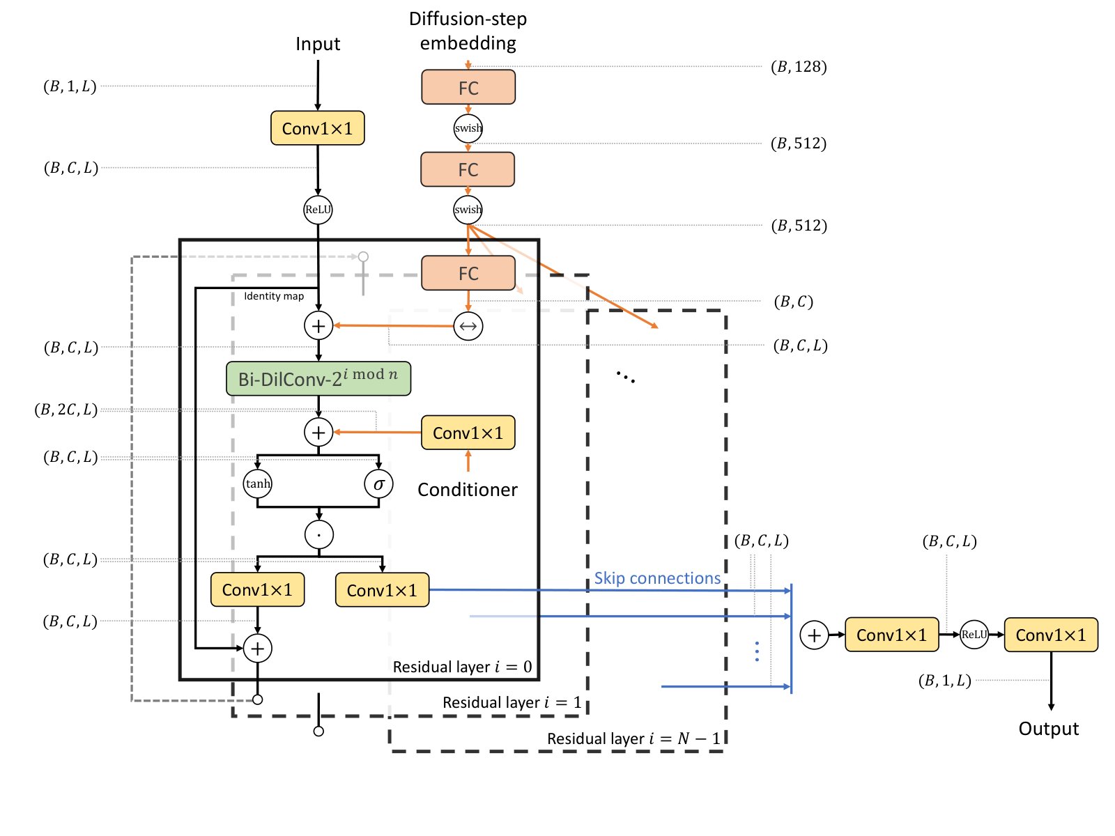
Figure 3: The network architecture of DiffWave in modeling , including tensor shapes at each stage and activation functions. is the batch size, is the number of residual/skip channels of the network, and is data dimension.
图 3:DiffWave 建模 的网络结构,含各阶段张量形状与激活函数。 为批大小, 为网络残差/跳跃通道数, 为数据维数。
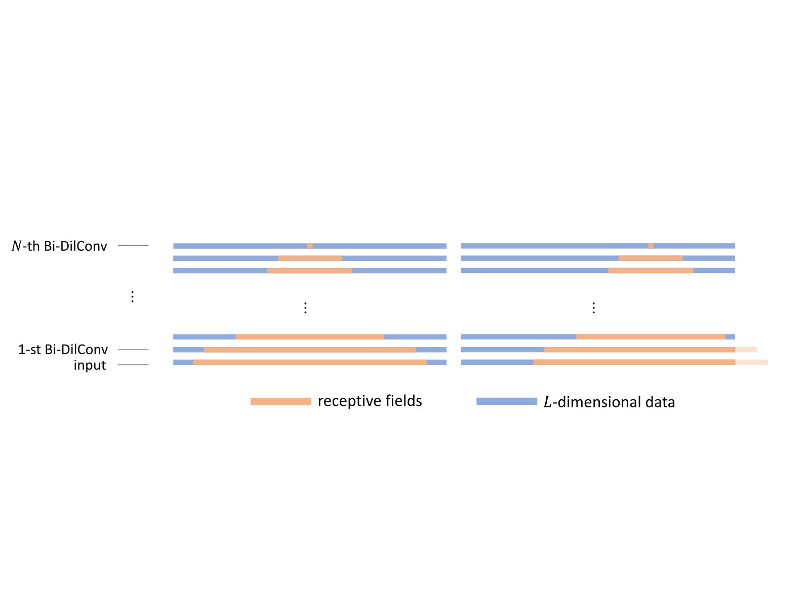
Figure 4: The Receptive fields of the output units within DiffWave network.
图 4:DiffWave 网络中输出单元的感受野。
Appendix D Details of Automatic Evaluation Metrics in Section 5.2 and 5.3
附录 D 第 5.2 与 5.3 节自动评测指标细节
The automatic evaluation metrics used in Section 5.2 and 5.3 are described as follows. Given an input audio , an 1024-dimensional feature vector (denoted as ) is computed by the ResNeXT , and is then transformed to the 10-dimensional multinomial distribution (denoted as ) with a fully connected layer and a softmax layer. Let be the trainset, be the distribution of generated data, and be the set of generated audio samples. Then, we compute the following automatic evaluation metrics:
第 5.2 与 5.3 节所用自动指标定义如下。给定输入音频 ,ResNeXT 算出 1024 维特征向量(记为 ),再经全连接与 softmax 变成 10 维多项分布(记为 )。令 为训练集, 为生成数据分布, 为生成样本集。则:
- • Fréchet Inception Distance (FID) (Heusel et al. 2017) computes the Wasserstein-2 distance between Gaussians fitted to and . That is, where are the mean vector and covariance matrix of , and where are the mean vector and covariance matrix of .
- • Fréchet Inception Distance(FID)(Heusel et al. 2017)计算拟合于 与 的高斯之间的 Wasserstein-2 距离,即 其中 为 的均值与协方差, 为 的均值与协方差。
- • Inception Score (IS) (Salimans et al. 2016) computes the following: where is the marginal label distribution.
- • Inception Score(IS)(Salimans et al. 2016)计算: 其中 为边缘标签分布。
- • Modified Inception Score (mIS) (Gurumurthy et al. 2017) computes the following:
- • Modified Inception Score(mIS)(Gurumurthy et al. 2017)计算:
- • AM Score (Zhou et al. 2017) computes the following: where computes the entropy. Compared to IS, AM score takes into consideration the the prior distribution of .
- • AM Score(Zhou et al. 2017)计算: 其中 为熵。相对 IS,AM 额外考虑 的先验分布。
- • Number of Statistically-Different Bins (NDB) (Richardson & Weiss 2018): First, is clustered into bins by -Means in the feature space (where in our evaluation). Next, each sample in is assigned to its nearest bin. Then, NDB is the number of bins that contain statistically different proportion of samples between training samples and generated samples.
- • Number of Statistically-Different Bins(NDB)(Richardson & Weiss 2018):先在特征空间用 -Means 把 聚成 个箱(本文评测取 );再把 中每个样本分到最近箱;NDB 为训练样本与生成样本比例在统计上显著不同的箱数。