Densely Connected Convolutional Networks

密集连接卷积网络（Densely Connected Convolutional Networks）

Gao Huang (Cornell University, gh349@cornell.edu), Zhuang Liu (Tsinghua University, liuzhuang13@mails.tsinghua.edu.cn), Laurens van der Maaten (Facebook AI Research, lvdmaaten@fb.com), Kilian Q. Weinberger (Cornell University, kqw4@cornell.edu)

* Authors contributed equally

黄高（康奈尔大学，gh349@cornell.edu）、刘壮（清华大学，liuzhuang13@mails.tsinghua.edu.cn）、Laurens van der Maaten（Facebook AI 研究院，lvdmaaten@fb.com）、Kilian Q. Weinberger（康奈尔大学，kqw4@cornell.edu）

* 两位作者贡献相同

Abstract

摘要

Recent work has shown that convolutional networks can be substantially deeper, more accurate, and efficient to train if they contain shorter connections between layers close to the input and those close to the output. In this paper, we embrace this observation and introduce the Dense Convolutional Network (DenseNet), which connects each layer to every other layer in a feed-forward fashion. Whereas traditional convolutional networks with $L$ layers have $L$ connections—one between each layer and its subsequent layer—our network has $\frac{L(L+1)}{2}$ direct connections. For each layer, the feature-maps of all preceding layers are used as inputs, and its own feature-maps are used as inputs into all subsequent layers. DenseNets have several compelling advantages: they alleviate the vanishing-gradient problem, strengthen feature propagation, encourage feature reuse, and substantially reduce the number of parameters. We evaluate our proposed architecture on four highly competitive object recognition benchmark tasks (CIFAR-10, CIFAR-100, SVHN, and ImageNet). DenseNets obtain significant improvements over the state-of-the-art on most of them, whilst requiring less computation to achieve high performance. Code and pre-trained models are available at https://github.com/liuzhuang13/DenseNet.

近来的研究表明，如果卷积网络在靠近输入的层和靠近输出的层之间有更短的连接，网络就可以做得更深、更准确，训练也更高效。本文沿着这一观察，提出密集卷积网络（Dense Convolutional Network，DenseNet）：它以前馈方式把每一层与其后的所有层相连。传统的 $L$ 层卷积网络有 $L$ 个连接，即每层与下一层之间各一个；我们的网络有 $\frac{L(L+1)}{2}$ 个直接连接。每一层都把之前所有层的特征图（feature-map）作为输入，自己的特征图又作为之后所有层的输入。DenseNet 有几项突出的优点：缓解梯度消失（vanishing-gradient）问题，加强特征传播，鼓励特征复用（feature reuse），并大幅减少参数量。我们在四个竞争激烈的物体识别基准任务（CIFAR-10、CIFAR-100、SVHN 和 ImageNet）上评估了这一架构。在其中大多数任务上，DenseNet 都比此前最好的结果有明显提升，同时达到高性能所需的计算量更少。代码和预训练模型见 https://github.com/liuzhuang13/DenseNet。

1 Introduction

1 引言

Convolutional neural networks (CNNs) have become the dominant machine learning approach for visual object recognition. Although they were originally introduced over 20 years ago [18], improvements in computer hardware and network structure have enabled the training of truly deep CNNs only recently. The original LeNet5 [19] consisted of 5 layers, VGG featured 19 [29], and only last year Highway Networks [34] and Residual Networks (ResNets) [11] have surpassed the 100-layer barrier.

卷积神经网络（CNN）已经成为视觉物体识别的主流机器学习方法。它最早在 20 多年前就已提出 [18]，但直到最近，计算机硬件和网络结构的改进才让真正的深层 CNN 训练成为可能。最初的 LeNet5 [19] 只有 5 层，VGG 有 19 层 [29]，直到去年，Highway Networks [34] 和残差网络（Residual Networks，ResNets）[11] 才突破了 100 层的门槛。

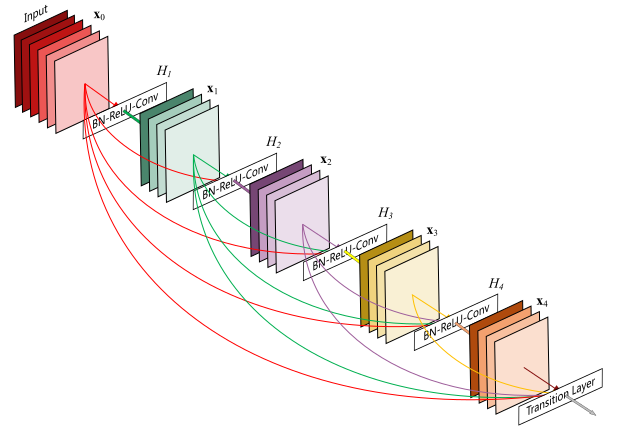
Figure 1: A 5-layer dense block with a growth rate of $k=4$. Each layer takes all preceding feature-maps as input.

图 1：一个增长率（growth rate）为 $k=4$ 的 5 层稠密块（dense block）。每一层都以之前所有的特征图作为输入。

As CNNs become increasingly deep, a new research problem emerges: as information about the input or gradient passes through many layers, it can vanish and “wash out” by the time it reaches the end (or beginning) of the network. Many recent publications address this or related problems. ResNets [11] and Highway Networks [34] bypass signal from one layer to the next via identity connections. Stochastic depth [13] shortens ResNets by randomly dropping layers during training to allow better information and gradient flow. FractalNets [17] repeatedly combine several parallel layer sequences with different number of convolutional blocks to obtain a large nominal depth, while maintaining many short paths in the network. Although these different approaches vary in network topology and training procedure, they all share a key characteristic: they create short paths from early layers to later layers.

随着 CNN 越来越深，出现了一个新的研究问题：输入信息或梯度在穿过许多层之后，到达网络末端（或起始端）时可能已经消失、被“冲淡”。近来许多论文都在处理这个问题或相关问题。ResNets [11] 和 Highway Networks [34] 通过恒等连接（identity connection）把信号从一层直接旁路到下一层。随机深度（Stochastic depth）[13] 在训练时随机丢弃层，缩短 ResNet，以改善信息和梯度的流动。FractalNets [17] 反复组合若干条卷积块数目不同的并行层序列，得到很大的名义深度，同时在网络中保留许多短路径。这些方法的网络拓扑和训练过程各不相同，但有一个共同的关键特征：都在靠前的层和靠后的层之间建立了短路径。

In this paper, we propose an architecture that distills this insight into a simple connectivity pattern: to ensure maximum information flow between layers in the network, we connect all layers (with matching feature-map sizes) directly with each other. To preserve the feed-forward nature, each layer obtains additional inputs from all preceding layers and passes on its own feature-maps to all subsequent layers. Figure 1 illustrates this layout schematically. Crucially, in contrast to ResNets, we never combine features through summation before they are passed into a layer; instead, we combine features by concatenating them. Hence, the $\ell^{th}$ layer has $\ell$ inputs, consisting of the feature-maps of all preceding convolutional blocks. Its own feature-maps are passed on to all $L-\ell$ subsequent layers. This introduces $\frac{L(L+1)}{2}$ connections in an $L$-layer network, instead of just $L$, as in traditional architectures. Because of its dense connectivity pattern, we refer to our approach as Dense Convolutional Network (DenseNet).

本文提出的架构把这一认识提炼成一种简单的连接模式：为了让网络各层之间的信息流动最大化，我们把（特征图尺寸相同的）所有层两两直接相连。为了保持前馈性质，每一层从之前所有层获得额外输入，并把自己的特征图传给之后所有层。图 1 是这种布局的示意。与 ResNet 的关键区别在于，我们从不在特征输入某一层之前把它们相加，而是把它们拼接（concatenate）起来。因此，第 $\ell$ 层有 $\ell$ 个输入，由之前所有卷积块的特征图组成；它自己的特征图则传给之后的全部 $L-\ell$ 层。这样，一个 $L$ 层网络就有 $\frac{L(L+1)}{2}$ 个连接，而不是传统架构中的 $L$ 个。由于这种稠密的连接模式，我们把这一方法称为密集卷积网络（DenseNet）。

A possibly counter-intuitive effect of this dense connectivity pattern is that it requires fewer parameters than traditional convolutional networks, as there is no need to re-learn redundant feature-maps. Traditional feed-forward architectures can be viewed as algorithms with a state, which is passed on from layer to layer. Each layer reads the state from its preceding layer and writes to the subsequent layer. It changes the state but also passes on information that needs to be preserved. ResNets [11] make this information preservation explicit through additive identity transformations. Recent variations of ResNets [13] show that many layers contribute very little and can in fact be randomly dropped during training. This makes the state of ResNets similar to (unrolled) recurrent neural networks [21], but the number of parameters of ResNets is substantially larger because each layer has its own weights. Our proposed DenseNet architecture explicitly differentiates between information that is added to the network and information that is preserved. DenseNet layers are very narrow (e.g., 12 filters per layer), adding only a small set of feature-maps to the “collective knowledge” of the network and keep the remaining feature-maps unchanged—and the final classifier makes a decision based on all feature-maps in the network.

这种稠密连接模式有一个可能违反直觉的效果：它需要的参数比传统卷积网络更少，因为网络不需要重新学习冗余的特征图。传统的前馈架构可以看作带有状态的算法，状态逐层传递。每一层从前一层读取状态，再写给下一层；它改变状态，同时也传递需要保留的信息。ResNets [11] 通过加性的恒等变换把这种信息保留显式化。ResNet 近来的变体 [13] 表明，许多层的贡献很小，训练中其实可以随机丢弃。这使 ResNet 的状态类似于（展开的）循环神经网络 [21]，但由于每层都有自己的权重，ResNet 的参数量要大得多。我们提出的 DenseNet 架构把新加入网络的信息和保留下来的信息明确区分开。DenseNet 的层非常窄（例如每层 12 个滤波器），只往网络的“集体知识”里加入一小组特征图，其余特征图保持不变；最终的分类器依据网络中的所有特征图做出决策。

Besides better parameter efficiency, one big advantage of DenseNets is their improved flow of information and gradients throughout the network, which makes them easy to train. Each layer has direct access to the gradients from the loss function and the original input signal, leading to an implicit deep supervision [20]. This helps training of deeper network architectures. Further, we also observe that dense connections have a regularizing effect, which reduces overfitting on tasks with smaller training set sizes.

除了参数效率更高，DenseNet 的另一大优势是整个网络中信息和梯度的流动更顺畅，因而容易训练。每一层都能直接获得来自损失函数的梯度和原始输入信号，形成一种隐式的深度监督（deep supervision）[20]。这有助于训练更深的网络架构。此外，我们还观察到稠密连接有正则化作用，能在训练集较小的任务上减轻过拟合。

We evaluate DenseNets on four highly competitive benchmark datasets (CIFAR-10, CIFAR-100, SVHN, and ImageNet). Our models tend to require much fewer parameters than existing algorithms with comparable accuracy. Further, we significantly outperform the current state-of-the-art results on most of the benchmark tasks.

我们在四个竞争激烈的基准数据集（CIFAR-10、CIFAR-100、SVHN 和 ImageNet）上评估 DenseNet。在精度相当的情况下，我们的模型所需的参数往往比现有算法少得多。此外，在大多数基准任务上，我们的结果明显超过了当前最好的结果。

Figure 2: A deep DenseNet with three dense blocks. The layers between two adjacent blocks are referred to as transition layers and change feature-map sizes via convolution and pooling.

图 2：一个包含三个稠密块的深层 DenseNet。两个相邻块之间的层称为过渡层（transition layer），它们通过卷积和池化改变特征图尺寸。

2 Related Work

2 相关工作

The exploration of network architectures has been a part of neural network research since their initial discovery. The recent resurgence in popularity of neural networks has also revived this research domain. The increasing number of layers in modern networks amplifies the differences between architectures and motivates the exploration of different connectivity patterns and the revisiting of old research ideas.

自神经网络最初被提出以来，网络架构的探索就一直是神经网络研究的一部分。近来神经网络重新流行，也让这一研究方向重新活跃起来。现代网络的层数不断增加，放大了不同架构之间的差异，促使人们探索不同的连接模式，并重新审视一些旧的研究思路。

A cascade structure similar to our proposed dense network layout has already been studied in the neural networks literature in the 1980s [3]. Their pioneering work focuses on fully connected multi-layer perceptrons trained in a layer-by-layer fashion. More recently, fully connected cascade networks to be trained with batch gradient descent were proposed [40]. Although effective on small datasets, this approach only scales to networks with a few hundred parameters. In [9, 23, 31, 41], utilizing multi-level features in CNNs through skip-connnections has been found to be effective for various vision tasks. Parallel to our work, [1] derived a purely theoretical framework for networks with cross-layer connections similar to ours.

与我们提出的稠密网络布局相似的级联结构，早在 20 世纪 80 年代的神经网络文献中就有人研究过 [3]。这项开创性工作关注逐层训练的全连接多层感知机。较近的工作提出了用批量梯度下降训练的全连接级联网络 [40]。这种方法在小数据集上有效，但只能扩展到参数量为几百的网络。在 [9, 23, 31, 41] 中，通过跳跃连接（skip-connection）在 CNN 中利用多层次特征，被证明对多种视觉任务有效。与我们的工作同期，[1] 为与我们相似的跨层连接网络推导了一个纯理论框架。

Highway Networks [34] were amongst the first architectures that provided a means to effectively train end-to-end networks with more than 100 layers. Using bypassing paths along with gating units, Highway Networks with hundreds of layers can be optimized without difficulty. The bypassing paths are presumed to be the key factor that eases the training of these very deep networks. This point is further supported by ResNets [11], in which pure identity mappings are used as bypassing paths. ResNets have achieved impressive, record-breaking performance on many challenging image recognition, localization, and detection tasks, such as ImageNet and COCO object detection [11]. Recently, stochastic depth was proposed as a way to successfully train a 1202-layer ResNet [13]. Stochastic depth improves the training of deep residual networks by dropping layers randomly during training. This shows that not all layers may be needed and highlights that there is a great amount of redundancy in deep (residual) networks. Our paper was partly inspired by that observation. ResNets with pre-activation also facilitate the training of state-of-the-art networks with $>$ 1000 layers [12].

Highway Networks [34] 是最早能够有效端到端训练 100 层以上网络的架构之一。借助旁路路径和门控单元，几百层的 Highway Networks 也能毫无困难地完成优化。人们认为旁路路径是让这些极深网络易于训练的关键因素。ResNets [11] 进一步支持了这一点，它直接用纯恒等映射作为旁路路径。ResNet 在 ImageNet、COCO 物体检测 [11] 等许多具有挑战性的图像识别、定位和检测任务上取得了令人瞩目的、破纪录的成绩。最近有人提出随机深度，成功训练了一个 1202 层的 ResNet [13]。随机深度在训练中随机丢弃层，改善了深度残差网络的训练。这说明并非所有层都是必需的，也凸显出深度（残差）网络中存在大量冗余。我们的论文部分受到了这一观察的启发。采用*预激活（pre-activation）*的 ResNet 也让超过 1000 层的最先进网络的训练变得更容易 [12]。

An orthogonal approach to making networks deeper (e.g., with the help of skip connections) is to increase the network width. The GoogLeNet [36, 37] uses an “Inception module” which concatenates feature-maps produced by filters of different sizes. In [38], a variant of ResNets with wide generalized residual blocks was proposed. In fact, simply increasing the number of filters in each layer of ResNets can improve its performance provided the depth is sufficient [42]. FractalNets also achieve competitive results on several datasets using a wide network structure [17].

与加深网络（例如借助跳跃连接）正交的另一条思路，是增加网络的宽度。GoogLeNet [36, 37] 使用“Inception 模块”，把不同尺寸滤波器产生的特征图拼接起来。[38] 提出了一种带有宽的广义残差块的 ResNet 变体。事实上，只要深度足够，单纯增加 ResNet 每层的滤波器数量就能提升性能 [42]。FractalNets 也用较宽的网络结构在若干数据集上取得了有竞争力的结果 [17]。

Instead of drawing representational power from extremely deep or wide architectures, DenseNets exploit the potential of the network through feature reuse, yielding condensed models that are easy to train and highly parameter-efficient. Concatenating feature-maps learned by different layers increases variation in the input of subsequent layers and improves efficiency. This constitutes a major difference between DenseNets and ResNets. Compared to Inception networks [36, 37], which also concatenate features from different layers, DenseNets are simpler and more efficient.

DenseNet 不靠极深或极宽的架构来获得表征能力，而是通过特征复用挖掘网络的潜力，得到紧凑、易训练、参数效率很高的模型。把不同层学到的特征图拼接起来，增加了后续层输入的多样性，也提高了效率。这是 DenseNet 和 ResNet 的一个主要区别。Inception 网络 [36, 37] 也会拼接不同层的特征，与之相比，DenseNet 更简单、更高效。

There are other notable network architecture innovations which have yielded competitive results. The Network in Network (NIN) [22] structure includes micro multi-layer perceptrons into the filters of convolutional layers to extract more complicated features. In Deeply Supervised Network (DSN) [20], internal layers are directly supervised by auxiliary classifiers, which can strengthen the gradients received by earlier layers. Ladder Networks [27, 25] introduce lateral connections into autoencoders, producing impressive accuracies on semi-supervised learning tasks. In [39], Deeply-Fused Nets (DFNs) were proposed to improve information flow by combining intermediate layers of different base networks. The augmentation of networks with pathways that minimize reconstruction losses was also shown to improve image classification models [43].

还有一些其他值得一提的网络架构创新也取得了有竞争力的结果。Network in Network（NIN）[22] 结构在卷积层的滤波器中加入微型多层感知机，以提取更复杂的特征。在深度监督网络（Deeply Supervised Network，DSN）[20] 中，内部各层直接由辅助分类器监督，这能增强靠前各层接收到的梯度。梯子网络（Ladder Networks）[27, 25] 在自编码器中引入横向连接，在半监督学习任务上取得了很高的精度。[39] 提出了深度融合网络（Deeply-Fused Nets，DFN），通过组合不同基础网络的中间层来改善信息流动。也有工作表明，给网络增加最小化重建损失的通路，可以改进图像分类模型 [43]。

Layers	Output Size	DenseNet-121	DenseNet-169	DenseNet-201	DenseNet-264
Convolution	112 × 112	7 × 7 conv, stride 2	7 × 7 conv, stride 2	7 × 7 conv, stride 2	7 × 7 conv, stride 2
Pooling	56 × 56	3 × 3 max pool, stride 2	3 × 3 max pool, stride 2	3 × 3 max pool, stride 2	3 × 3 max pool, stride 2
Dense Block (1)	56 × 56	[1 × 1 conv, 3 × 3 conv] × 6	[1 × 1 conv, 3 × 3 conv] × 6	[1 × 1 conv, 3 × 3 conv] × 6	[1 × 1 conv, 3 × 3 conv] × 6
Transition Layer (1)	56 × 56	1 × 1 conv	1 × 1 conv	1 × 1 conv	1 × 1 conv
	28 × 28	2 × 2 average pool, stride 2	2 × 2 average pool, stride 2	2 × 2 average pool, stride 2	2 × 2 average pool, stride 2
Dense Block (2)	28 × 28	[1 × 1 conv, 3 × 3 conv] × 12	[1 × 1 conv, 3 × 3 conv] × 12	[1 × 1 conv, 3 × 3 conv] × 12	[1 × 1 conv, 3 × 3 conv] × 12
Transition Layer (2)	28 × 28	1 × 1 conv	1 × 1 conv	1 × 1 conv	1 × 1 conv
	14 × 14	2 × 2 average pool, stride 2	2 × 2 average pool, stride 2	2 × 2 average pool, stride 2	2 × 2 average pool, stride 2
Dense Block (3)	14 × 14	[1 × 1 conv, 3 × 3 conv] × 24	[1 × 1 conv, 3 × 3 conv] × 32	[1 × 1 conv, 3 × 3 conv] × 48	[1 × 1 conv, 3 × 3 conv] × 64
Transition Layer (3)	14 × 14	1 × 1 conv	1 × 1 conv	1 × 1 conv	1 × 1 conv
	7 × 7	2 × 2 average pool, stride 2	2 × 2 average pool, stride 2	2 × 2 average pool, stride 2	2 × 2 average pool, stride 2
Dense Block (4)	7 × 7	[1 × 1 conv, 3 × 3 conv] × 16	[1 × 1 conv, 3 × 3 conv] × 32	[1 × 1 conv, 3 × 3 conv] × 32	[1 × 1 conv, 3 × 3 conv] × 48
Classification Layer	1 × 1	7 × 7 global average pool	7 × 7 global average pool	7 × 7 global average pool	7 × 7 global average pool
		1000D fully-connected, softmax	1000D fully-connected, softmax	1000D fully-connected, softmax	1000D fully-connected, softmax

Table 1: DenseNet architectures for ImageNet. The growth rate for all the networks is $k=32$. Note that each “conv” layer shown in the table corresponds the sequence BN-ReLU-Conv.

层	输出尺寸	DenseNet-121	DenseNet-169	DenseNet-201	DenseNet-264
卷积	112 × 112	7 × 7 卷积，步长 2	7 × 7 卷积，步长 2	7 × 7 卷积，步长 2	7 × 7 卷积，步长 2
池化	56 × 56	3 × 3 最大池化，步长 2	3 × 3 最大池化，步长 2	3 × 3 最大池化，步长 2	3 × 3 最大池化，步长 2
稠密块（1）	56 × 56	[1 × 1 卷积, 3 × 3 卷积] × 6	[1 × 1 卷积, 3 × 3 卷积] × 6	[1 × 1 卷积, 3 × 3 卷积] × 6	[1 × 1 卷积, 3 × 3 卷积] × 6
过渡层（1）	56 × 56	1 × 1 卷积	1 × 1 卷积	1 × 1 卷积	1 × 1 卷积
	28 × 28	2 × 2 平均池化，步长 2	2 × 2 平均池化，步长 2	2 × 2 平均池化，步长 2	2 × 2 平均池化，步长 2
稠密块（2）	28 × 28	[1 × 1 卷积, 3 × 3 卷积] × 12	[1 × 1 卷积, 3 × 3 卷积] × 12	[1 × 1 卷积, 3 × 3 卷积] × 12	[1 × 1 卷积, 3 × 3 卷积] × 12
过渡层（2）	28 × 28	1 × 1 卷积	1 × 1 卷积	1 × 1 卷积	1 × 1 卷积
	14 × 14	2 × 2 平均池化，步长 2	2 × 2 平均池化，步长 2	2 × 2 平均池化，步长 2	2 × 2 平均池化，步长 2
稠密块（3）	14 × 14	[1 × 1 卷积, 3 × 3 卷积] × 24	[1 × 1 卷积, 3 × 3 卷积] × 32	[1 × 1 卷积, 3 × 3 卷积] × 48	[1 × 1 卷积, 3 × 3 卷积] × 64
过渡层（3）	14 × 14	1 × 1 卷积	1 × 1 卷积	1 × 1 卷积	1 × 1 卷积
	7 × 7	2 × 2 平均池化，步长 2	2 × 2 平均池化，步长 2	2 × 2 平均池化，步长 2	2 × 2 平均池化，步长 2
稠密块（4）	7 × 7	[1 × 1 卷积, 3 × 3 卷积] × 16	[1 × 1 卷积, 3 × 3 卷积] × 32	[1 × 1 卷积, 3 × 3 卷积] × 32	[1 × 1 卷积, 3 × 3 卷积] × 48
分类层	1 × 1	7 × 7 全局平均池化	7 × 7 全局平均池化	7 × 7 全局平均池化	7 × 7 全局平均池化
		1000 维全连接，softmax	1000 维全连接，softmax	1000 维全连接，softmax	1000 维全连接，softmax

表 1：用于 ImageNet 的 DenseNet 架构。所有网络的增长率均为 $k=32$。注意，表中每个“卷积”层都对应 BN-ReLU-Conv 这一操作序列。

3 DenseNets

3 DenseNet

Consider a single image $\mathbf{x}_{0}$ that is passed through a convolutional network. The network comprises $L$ layers, each of which implements a non-linear transformation $H_{\ell}(\cdot)$, where $\ell$ indexes the layer. $H_{\ell}(\cdot)$ can be a composite function of operations such as Batch Normalization (BN) [14], rectified linear units (ReLU) [6], Pooling [19], or Convolution (Conv). We denote the output of the $\ell^{th}$ layer as $\mathbf{x}_{\ell}$.

设有一张图像 $\mathbf{x}_{0}$ 输入卷积网络。网络由 $L$ 层组成，每层实现一个非线性变换 $H_{\ell}(\cdot)$，其中 $\ell$ 是层的编号。$H_{\ell}(\cdot)$ 可以是批归一化（Batch Normalization，BN）[14]、线性整流单元（ReLU）[6]、池化（Pooling）[19] 或卷积（Conv）等操作的复合函数。我们把第 $\ell$ 层的输出记为 $\mathbf{x}_{\ell}$。

ResNets.

Traditional convolutional feed-forward networks connect the output of the $\ell^{th}$ layer as input to the $(\ell+1)^{th}$ layer [16], which gives rise to the following layer transition: $\mathbf{x}_{\ell}=H_{\ell}(\mathbf{x}_{\ell-1})$. ResNets [11] add a skip-connection that bypasses the non-linear transformations with an identity function:

ResNets。

传统的前馈卷积网络把第 $\ell$ 层的输出作为第 $(\ell+1)$ 层的输入 [16]，由此得到如下的层间转换：$\mathbf{x}_{\ell}=H_{\ell}(\mathbf{x}_{\ell-1})$。ResNets [11] 增加了一条跳跃连接，用恒等函数绕过非线性变换：

$$\mathbf{x}_{\ell}=H_{\ell}(\mathbf{x}_{\ell-1})+\mathbf{x}_{\ell-1}. \tag{1}$$

An advantage of ResNets is that the gradient can flow directly through the identity function from later layers to the earlier layers. However, the identity function and the output of $H_{\ell}$ are combined by summation, which may impede the information flow in the network.

ResNet 的一个优点是，梯度可以经由恒等函数从靠后的层直接流向靠前的层。不过，恒等函数和 $H_{\ell}$ 的输出是相加合并的，这可能阻碍网络中的信息流动。

Dense connectivity.

To further improve the information flow between layers we propose a different connectivity pattern: we introduce direct connections from any layer to all subsequent layers. Figure 1 illustrates the layout of the resulting DenseNet schematically. Consequently, the $\ell^{th}$ layer receives the feature-maps of all preceding layers, $\mathbf{x}_{0},\dots,\mathbf{x}_{\ell-1}$, as input:

稠密连接。

为了进一步改善层间的信息流动，我们提出一种不同的连接模式：从任一层到其后所有层都引入直接连接。图 1 是由此得到的 DenseNet 布局示意。于是，第 $\ell$ 层接收之前所有层的特征图 $\mathbf{x}_{0},\dots,\mathbf{x}_{\ell-1}$ 作为输入：

$$\mathbf{x}_{\ell}=\ H_{\ell}([\mathbf{x}_{0},\mathbf{x}_{1},\ldots,\mathbf{x}_{\ell-1}]), \tag{2}$$

where $[\mathbf{x}_{0},\mathbf{x}_{1},\ldots,\mathbf{x}_{\ell-1}]$ refers to the concatenation of the feature-maps produced in layers $0,\dots,\ell-1$. Because of its dense connectivity we refer to this network architecture as Dense Convolutional Network (DenseNet). For ease of implementation, we concatenate the multiple inputs of $H_{\ell}(\cdot)$ in eq. (2) into a single tensor.

其中 $[\mathbf{x}_{0},\mathbf{x}_{1},\ldots,\mathbf{x}_{\ell-1}]$ 表示第 $0,\dots,\ell-1$ 层所产生特征图的拼接。由于这种稠密连接，我们把这种网络架构称为密集卷积网络（DenseNet）。为了便于实现，我们把式 (2) 中 $H_{\ell}(\cdot)$ 的多个输入拼接成单个张量。

Composite function.

Motivated by [12], we define $H_{\ell}(\cdot)$ as a composite function of three consecutive operations: batch normalization (BN) [14], followed by a rectified linear unit (ReLU) [6] and a $3\times 3$ convolution (Conv).

复合函数。

受 [12] 启发，我们把 $H_{\ell}(\cdot)$ 定义为三个连续操作的复合函数：批归一化（BN）[14]，接着是线性整流单元（ReLU）[6] 和一个 $3\times 3$ 卷积（Conv）。

Pooling layers.

The concatenation operation used in Eq. (2) is not viable when the size of feature-maps changes. However, an essential part of convolutional networks is down-sampling layers that change the size of feature-maps. To facilitate down-sampling in our architecture we divide the network into multiple densely connected dense blocks; see Figure 2. We refer to layers between blocks as transition layers, which do convolution and pooling. The transition layers used in our experiments consist of a batch normalization layer and an 1$\times$1 convolutional layer followed by a 2$\times$2 average pooling layer.

池化层。

当特征图尺寸发生变化时，式 (2) 中的拼接操作就无法进行。然而，改变特征图尺寸的下采样层是卷积网络的必要组成部分。为了在架构中实现下采样，我们把网络划分为多个内部稠密连接的稠密块，见图 2。块与块之间的层称为过渡层，负责卷积和池化。实验中使用的过渡层由一个批归一化层、一个 1$\times$1 卷积层和其后的一个 2$\times$2 平均池化层组成。

Growth rate.

If each function $H_{\ell}$ produces $k$ feature-maps, it follows that the $\ell^{th}$ layer has $k_{0}+k\times(\ell-1)$ input feature-maps, where $k_{0}$ is the number of channels in the input layer. An important difference between DenseNet and existing network architectures is that DenseNet can have very narrow layers, e.g., $k=12$. We refer to the hyper-parameter $k$ as the growth rate of the network. We show in Section 2 that a relatively small growth rate is sufficient to obtain state-of-the-art results on the datasets that we tested on. One explanation for this is that each layer has access to all the preceding feature-maps in its block and, therefore, to the network’s “collective knowledge”. One can view the feature-maps as the global state of the network. Each layer adds $k$ feature-maps of its own to this state. The growth rate regulates how much new information each layer contributes to the global state. The global state, once written, can be accessed from everywhere within the network and, unlike in traditional network architectures, there is no need to replicate it from layer to layer.

增长率。

如果每个函数 $H_{\ell}$ 产生 $k$ 个特征图，那么第 $\ell$ 层就有 $k_{0}+k\times(\ell-1)$ 个输入特征图，其中 $k_{0}$ 是输入层的通道数。DenseNet 与现有网络架构的一个重要区别在于，DenseNet 的层可以非常窄，例如 $k=12$。我们把超参数 $k$ 称为网络的增长率。第 2 节表明，在我们测试的数据集上，相对较小的增长率就足以取得最先进的结果。一种解释是，每一层都能访问所在块中之前所有的特征图，也就能访问网络的“集体知识”。可以把特征图看作网络的全局状态，每一层往这个状态里加入自己的 $k$ 个特征图。增长率控制每一层向全局状态贡献多少新信息。全局状态一旦写入，网络中任何位置都能访问；与传统网络架构不同，它不需要逐层复制。

Bottleneck layers.

Although each layer only produces $k$ output feature-maps, it typically has many more inputs. It has been noted in [37, 11] that a 1$\times$1 convolution can be introduced as bottleneck layer before each 3$\times$3 convolution to reduce the number of input feature-maps, and thus to improve computational efficiency. We find this design especially effective for DenseNet and we refer to our network with such a bottleneck layer, i.e., to the BN-ReLU-Conv(1$\times$ 1)-BN-ReLU-Conv(3$\times$3) version of $H_{\ell}$, as DenseNet-B. In our experiments, we let each 1$\times$1 convolution produce $4k$ feature-maps.

瓶颈层。

每一层虽然只产生 $k$ 个输出特征图，输入通常却多得多。[37, 11] 指出，可以在每个 3$\times$3 卷积之前引入一个 1$\times$1 卷积作为瓶颈层（bottleneck layer），减少输入特征图的数量，从而提高计算效率。我们发现这一设计对 DenseNet 特别有效。我们把带有这种瓶颈层的网络，即 $H_{\ell}$ 采用 BN-ReLU-Conv(1$\times$ 1)-BN-ReLU-Conv(3$\times$3) 形式的版本，称为 DenseNet-B。实验中，我们让每个 1$\times$1 卷积产生 $4k$ 个特征图。

Compression.

To further improve model compactness, we can reduce the number of feature-maps at transition layers. If a dense block contains $m$ feature-maps, we let the following transition layer generate $\lfloor\theta m\rfloor$ output feature-maps, where $0<\!\theta\leq\!1$ is referred to as the compression factor. When $\theta\!=\!1$, the number of feature-maps across transition layers remains unchanged. We refer the DenseNet with $\theta\!<\!1$ as DenseNet-C, and we set $\theta=0.5$ in our experiment. When both the bottleneck and transition layers with $\theta\!<1$ are used, we refer to our model as DenseNet-BC.

压缩。

为了让模型更紧凑，可以在过渡层减少特征图的数量。如果一个稠密块包含 $m$ 个特征图，我们让其后的过渡层生成 $\lfloor\theta m\rfloor$ 个输出特征图，其中 $0<\!\theta\leq\!1$ 称为压缩因子（compression factor）。当 $\theta\!=\!1$ 时，经过过渡层的特征图数量保持不变。我们把 $\theta\!<\!1$ 的 DenseNet 称为 DenseNet-C，实验中设 $\theta=0.5$。同时使用瓶颈层和 $\theta\!<1$ 的过渡层时，我们把模型称为 DenseNet-BC。

Implementation Details.

On all datasets except ImageNet, the DenseNet used in our experiments has three dense blocks that each has an equal number of layers. Before entering the first dense block, a convolution with 16 (or twice the growth rate for DenseNet-BC) output channels is performed on the input images. For convolutional layers with kernel size 3$\times$3, each side of the inputs is zero-padded by one pixel to keep the feature-map size fixed. We use 1$\times$1 convolution followed by 2$\times$2 average pooling as transition layers between two contiguous dense blocks. At the end of the last dense block, a global average pooling is performed and then a softmax classifier is attached. The feature-map sizes in the three dense blocks are 32$\times$ 32, 16$\times$16, and 8$\times$8, respectively. We experiment with the basic DenseNet structure with configurations $\{L\!=\!40,k\!=\!12\}$, $\{L\!=\!100,k\!=\!12\}$ and $\{L\!=\!100,k\!=\!24\}$. For DenseNet-BC, the networks with configurations $\{L\!=\!100,k\!=\!12\}$, $\{L\!=\!250,k\!=\!24\}$ and $\{L\!=\!190,k\!=\!40\}$ are evaluated.

实现细节。

在 ImageNet 以外的所有数据集上，实验所用的 DenseNet 都有三个层数相同的稠密块。进入第一个稠密块之前，先对输入图像做一次输出通道数为 16（DenseNet-BC 则为增长率的两倍）的卷积。对于卷积核为 3$\times$3 的卷积层，输入的每条边补一个像素的零，以保持特征图尺寸不变。两个相邻稠密块之间的过渡层采用 1$\times$1 卷积加 2$\times$2 平均池化。最后一个稠密块之后做一次全局平均池化，再接一个 softmax 分类器。三个稠密块中的特征图尺寸分别为 32$\times$ 32、16$\times$16 和 8$\times$8。基本 DenseNet 结构我们试验了 $\{L\!=\!40,k\!=\!12\}$、$\{L\!=\!100,k\!=\!12\}$ 和 $\{L\!=\!100,k\!=\!24\}$ 三种配置。DenseNet-BC 评估了 $\{L\!=\!100,k\!=\!12\}$、$\{L\!=\!250,k\!=\!24\}$ 和 $\{L\!=\!190,k\!=\!40\}$ 三种配置。

In our experiments on ImageNet, we use a DenseNet-BC structure with 4 dense blocks on 224$\times$224 input images. The initial convolution layer comprises $2k$ convolutions of size 7$\times$7 with stride 2; the number of feature-maps in all other layers also follow from setting $k$. The exact network configurations we used on ImageNet are shown in Table 1.

在 ImageNet 实验中，我们在 224$\times$224 的输入图像上使用含 4 个稠密块的 DenseNet-BC 结构。初始卷积层由 $2k$ 个步长为 2 的 7$\times$7 卷积组成；其他所有层的特征图数量也都由 $k$ 的设定决定。我们在 ImageNet 上使用的具体网络配置见表 1。

4 Experiments

4 实验

Method	Depth	Params	C10	C10+	C100	C100+	SVHN
Network in Network [22]	-	-	10.41	8.81	35.68	-	2.35
All-CNN [32]	-	-	9.08	7.25	-	33.71	-
Deeply Supervised Net [20]	-	-	9.69	7.97	-	34.57	1.92
Highway Network [34]	-	-	-	7.72	-	32.39	-
FractalNet [17]	21	38.6M	10.18	5.22	35.34	23.30	2.01
with Dropout/Drop-path	21	38.6M	7.33	4.60	28.20	23.73	1.87
ResNet [11]	110	1.7M	-	6.61	-	-	-
ResNet (reported by [13])	110	1.7M	13.63	6.41	44.74	27.22	2.01
ResNet with Stochastic Depth [13]	110	1.7M	11.66	5.23	37.80	24.58	1.75
	1202	10.2M	-	4.91	-	-	-
Wide ResNet [42]	16	11.0M	-	4.81	-	22.07	-
	28	36.5M	-	4.17	-	20.50	-
with Dropout	16	2.7M	-	-	-	-	1.64
ResNet (pre-activation) [12]	164	1.7M	11.26∗	5.46	35.58∗	24.33	-
	1001	10.2M	10.56∗	4.62	33.47∗	22.71	-
DenseNet $(k=12)$	40	1.0M	7.00	5.24	27.55	24.42	1.79
DenseNet $(k=12)$	100	7.0M	5.77	4.10	23.79	20.20	1.67
DenseNet $(k=24)$	100	27.2M	5.83	3.74	23.42	19.25	1.59
DenseNet-BC $(k=12)$	100	0.8M	5.92	4.51	24.15	22.27	1.76
DenseNet-BC $(k=24)$	250	15.3M	5.19	3.62	19.64	17.60	1.74
DenseNet-BC $(k=40)$	190	25.6M	-	3.46	-	17.18	-

Table 2: Error rates (%) on CIFAR and SVHN datasets. $k$ denotes network’s growth rate. Results that surpass all competing methods are bold and the overall best results are blue. “+” indicates standard data augmentation (translation and/or mirroring). $\ast$ indicates results run by ourselves. All the results of DenseNets without data augmentation (C10, C100, SVHN) are obtained using Dropout. DenseNets achieve lower error rates while using fewer parameters than ResNet. Without data augmentation, DenseNet performs better by a large margin.

方法	深度	参数量	C10	C10+	C100	C100+	SVHN
Network in Network [22]	-	-	10.41	8.81	35.68	-	2.35
All-CNN [32]	-	-	9.08	7.25	-	33.71	-
Deeply Supervised Net [20]	-	-	9.69	7.97	-	34.57	1.92
Highway Network [34]	-	-	-	7.72	-	32.39	-
FractalNet [17]	21	38.6M	10.18	5.22	35.34	23.30	2.01
加 Dropout/Drop-path	21	38.6M	7.33	4.60	28.20	23.73	1.87
ResNet [11]	110	1.7M	-	6.61	-	-	-
ResNet（[13] 报告的结果）	110	1.7M	13.63	6.41	44.74	27.22	2.01
带随机深度的 ResNet [13]	110	1.7M	11.66	5.23	37.80	24.58	1.75
	1202	10.2M	-	4.91	-	-	-
Wide ResNet [42]	16	11.0M	-	4.81	-	22.07	-
	28	36.5M	-	4.17	-	20.50	-
加 Dropout	16	2.7M	-	-	-	-	1.64
ResNet（预激活）[12]	164	1.7M	11.26∗	5.46	35.58∗	24.33	-
	1001	10.2M	10.56∗	4.62	33.47∗	22.71	-
DenseNet $(k=12)$	40	1.0M	7.00	5.24	27.55	24.42	1.79
DenseNet $(k=12)$	100	7.0M	5.77	4.10	23.79	20.20	1.67
DenseNet $(k=24)$	100	27.2M	5.83	3.74	23.42	19.25	1.59
DenseNet-BC $(k=12)$	100	0.8M	5.92	4.51	24.15	22.27	1.76
DenseNet-BC $(k=24)$	250	15.3M	5.19	3.62	19.64	17.60	1.74
DenseNet-BC $(k=40)$	190	25.6M	-	3.46	-	17.18	-

表 2：CIFAR 和 SVHN 数据集上的错误率（%）。$k$ 表示网络的增长率。超过所有对比方法的结果用粗体标出，总体最好的结果用蓝色标出（原文以颜色区分）。“+”表示使用了标准数据增强（平移和/或镜像）。$\ast$ 表示由我们自己运行得到的结果。DenseNet 在不做数据增强的设置（C10、C100、SVHN）下的结果都使用了 Dropout。DenseNet 的参数比 ResNet 少，错误率却更低。不做数据增强时，DenseNet 的优势更大。

We empirically demonstrate DenseNet’s effectiveness on several benchmark datasets and compare with state-of-the-art architectures, especially with ResNet and its variants.

我们在几个基准数据集上实证检验 DenseNet 的有效性，并与最先进的架构比较，尤其是 ResNet 及其变体。

4.1 Datasets

4.1 数据集

CIFAR.

The two CIFAR datasets [15] consist of colored natural images with 32$\times$32 pixels. CIFAR-10 (C10) consists of images drawn from 10 and CIFAR-100 (C100) from 100 classes. The training and test sets contain 50,000 and 10,000 images respectively, and we hold out 5,000 training images as a validation set. We adopt a standard data augmentation scheme (mirroring/shifting) that is widely used for these two datasets [11, 13, 17, 22, 28, 20, 32, 34]. We denote this data augmentation scheme by a “+” mark at the end of the dataset name (e.g., C10+). For preprocessing, we normalize the data using the channel means and standard deviations. For the final run we use all 50,000 training images and report the final test error at the end of training.

CIFAR。

两个 CIFAR 数据集 [15] 由 32$\times$32 像素的彩色自然图像组成。CIFAR-10（C10）的图像来自 10 个类别，CIFAR-100（C100）来自 100 个类别。训练集和测试集分别有 50,000 和 10,000 张图像，我们从训练图像中留出 5,000 张作为验证集。我们采用这两个数据集上广泛使用的标准数据增强方案（镜像/平移）[11, 13, 17, 22, 28, 20, 32, 34]，并在数据集名称末尾加“+”号表示使用了这一方案（例如 C10+）。预处理时，我们用各通道的均值和标准差对数据做归一化。最终一轮训练使用全部 50,000 张训练图像，并报告训练结束时的测试误差。

SVHN.

The Street View House Numbers (SVHN) dataset [24] contains 32$\times$32 colored digit images. There are 73,257 images in the training set, 26,032 images in the test set, and 531,131 images for additional training. Following common practice [7, 13, 20, 22, 30] we use all the training data without any data augmentation, and a validation set with 6,000 images is split from the training set. We select the model with the lowest validation error during training and report the test error. We follow [42] and divide the pixel values by 255 so they are in the $[0,1]$ range.

SVHN。

街景门牌号（Street View House Numbers，SVHN）数据集 [24] 包含 32$\times$32 的彩色数字图像。训练集有 73,257 张图像，测试集有 26,032 张，另有 531,131 张作为额外训练数据。按照通行做法 [7, 13, 20, 22, 30]，我们使用全部训练数据，不做任何数据增强，并从训练集中划出 6,000 张图像作为验证集。我们选取训练过程中验证误差最低的模型，报告其测试误差。我们沿用 [42] 的做法，把像素值除以 255，使其落在 $[0,1]$ 区间内。

Model	top-1	top-5
DenseNet-121	25.02 / 23.61	7.71 / 6.66
DenseNet-169	23.80 / 22.08	6.85 / 5.92
DenseNet-201	22.58 / 21.46	6.34 / 5.54
DenseNet-264	22.15 / 20.80	6.12 / 5.29

Table 3: The top-1 and top-5 error rates on the ImageNet validation set, with single-crop / 10-crop testing.

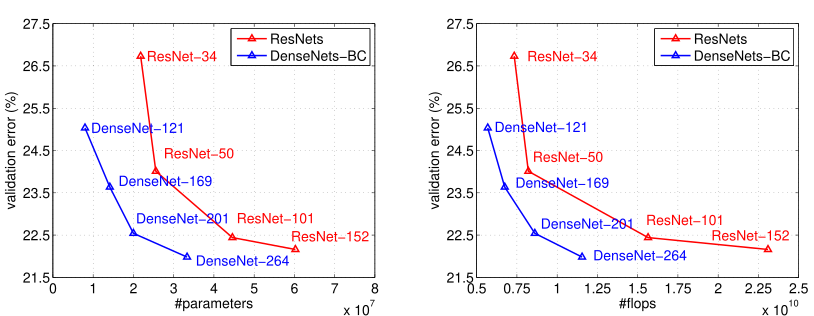
Figure 3: Comparison of the DenseNets and ResNets top-1 error rates (single-crop testing) on the ImageNet validation dataset as a function of learned parameters (left) and FLOPs during test-time (right).

模型	top-1	top-5
DenseNet-121	25.02 / 23.61	7.71 / 6.66
DenseNet-169	23.80 / 22.08	6.85 / 5.92
DenseNet-201	22.58 / 21.46	6.34 / 5.54
DenseNet-264	22.15 / 20.80	6.12 / 5.29

表 3：ImageNet 验证集上的 top-1 和 top-5 错误率，分别为单裁剪 / 10 裁剪（10-crop）测试的结果。

图 3：DenseNet 与 ResNet 在 ImageNet 验证集上的 top-1 错误率（单裁剪测试）对比，横轴分别为学习到的参数量（左）和测试时的 FLOPs（右）。

ImageNet.

The ILSVRC 2012 classification dataset [2] consists 1.2 million images for training, and 50,000 for validation, from $1,000$ classes. We adopt the same data augmentation scheme for training images as in [8, 11, 12], and apply a single-crop or 10-crop with size 224$\times$224 at test time. Following [11, 12, 13], we report classification errors on the validation set.

ImageNet。

ILSVRC 2012 分类数据集 [2] 包含来自 $1,000$ 个类别的 120 万张训练图像和 50,000 张验证图像。训练图像的数据增强方案与 [8, 11, 12] 相同，测试时采用 224$\times$224 的单裁剪或 10 裁剪。按照 [11, 12, 13] 的做法，我们报告验证集上的分类错误率。

4.2 Training

4.2 训练

All the networks are trained using stochastic gradient descent (SGD). On CIFAR and SVHN we train using batch size 64 for 300 and 40 epochs, respectively. The initial learning rate is set to 0.1, and is divided by 10 at 50% and 75% of the total number of training epochs. On ImageNet, we train models for 90 epochs with a batch size of 256. The learning rate is set to 0.1 initially, and is lowered by 10 times at epoch 30 and 60. Note that a naive implementation of DenseNet may contain memory inefficiencies. To reduce the memory consumption on GPUs, please refer to our technical report on the memory-efficient implementation of DenseNets [26].

所有网络都用随机梯度下降（SGD）训练。在 CIFAR 和 SVHN 上，批大小为 64，分别训练 300 和 40 个轮次（epoch）。初始学习率设为 0.1，在训练总轮次的 50% 和 75% 处各除以 10。在 ImageNet 上，我们以 256 的批大小训练 90 个轮次。学习率初始为 0.1，在第 30 和第 60 个轮次各降为原来的十分之一。注意，DenseNet 的朴素实现可能存在内存使用效率不高的问题。如需降低 GPU 内存消耗，请参阅我们关于 DenseNet 内存高效实现的技术报告 [26]。

Following [8], we use a weight decay of $10^{-4}$ and a Nesterov momentum [35] of 0.9 without dampening. We adopt the weight initialization introduced by [10]. For the three datasets without data augmentation, i.e., C10, C100 and SVHN, we add a dropout layer [33] after each convolutional layer (except the first one) and set the dropout rate to 0.2. The test errors were only evaluated once for each task and model setting.

沿用 [8] 的设置，我们使用 $10^{-4}$ 的权重衰减和 0.9 的 Nesterov 动量 [35]，不加阻尼（dampening）。权重初始化采用 [10] 提出的方法。对于不做数据增强的三个数据集，即 C10、C100 和 SVHN，我们在每个卷积层（第一个除外）之后加一个 dropout 层 [33]，dropout 率设为 0.2。每项任务和每种模型设置的测试误差都只评估一次。

4.3 Classification Results on CIFAR and SVHN

4.3 CIFAR 和 SVHN 上的分类结果

We train DenseNets with different depths, $L$, and growth rates, $k$. The main results on CIFAR and SVHN are shown in Table 2. To highlight general trends, we mark all results that outperform the existing state-of-the-art in boldface and the overall best result in blue.

我们训练了不同深度 $L$ 和不同增长率 $k$ 的 DenseNet。CIFAR 和 SVHN 上的主要结果见表 2。为了突出总体趋势，我们把所有超过现有最好结果的数字标为粗体，把总体最好的结果标为蓝色。

Accuracy.

Possibly the most noticeable trend may originate from the bottom row of Table 2, which shows that DenseNet-BC with $L\!=\!190$ and $k\!=\!40$ outperforms the existing state-of-the-art consistently on all the CIFAR datasets. Its error rates of 3.46% on C10+ and 17.18% on C100+ are significantly lower than the error rates achieved by wide ResNet architecture [42]. Our best results on C10 and C100 (without data augmentation) are even more encouraging: both are close to 30% lower than FractalNet with drop-path regularization [17]. On SVHN, with dropout, the DenseNet with $L\!=\!100$ and $k\!=\!24$ also surpasses the current best result achieved by wide ResNet. However, the 250-layer DenseNet-BC doesn’t further improve the performance over its shorter counterpart. This may be explained by that SVHN is a relatively easy task, and extremely deep models may overfit to the training set.

精度。

最明显的趋势可能来自表 2 的最后一行：$L\!=\!190$、$k\!=\!40$ 的 DenseNet-BC 在所有 CIFAR 数据集上都稳定超过现有最好结果。它在 C10+ 上 3.46% 和 C100+ 上 17.18% 的错误率，明显低于宽残差网络（wide ResNet）架构 [42] 的错误率。我们在 C10 和 C100（不做数据增强）上的最好结果更令人鼓舞：两者都比使用 drop-path 正则化的 FractalNet [17] 低近 30%。在 SVHN 上，使用 dropout 的 $L\!=\!100$、$k\!=\!24$ 的 DenseNet 也超过了宽残差网络取得的当前最好结果。不过，250 层的 DenseNet-BC 并没有比更浅的版本进一步提升性能。一个可能的解释是，SVHN 相对简单，极深的模型可能会过拟合训练集。

Capacity.

Without compression or bottleneck layers, there is a general trend that DenseNets perform better as $L$ and $k$ increase. We attribute this primarily to the corresponding growth in model capacity. This is best demonstrated by the column of C10+ and C100+. On C10+, the error drops from 5.24% to 4.10% and finally to 3.74% as the number of parameters increases from 1.0M, over 7.0M to 27.2M. On C100+, we observe a similar trend. This suggests that DenseNets can utilize the increased representational power of bigger and deeper models. It also indicates that they do not suffer from overfitting or the optimization difficulties of residual networks [11].

容量。

在不使用压缩或瓶颈层时，总体趋势是 $L$ 和 $k$ 越大，DenseNet 表现越好。我们认为这主要源于相应增加的模型容量。C10+ 和 C100+ 两列最能说明这一点。在 C10+ 上，随着参数量从 1.0M 增加到 7.0M 再到 27.2M，错误率从 5.24% 降到 4.10%，最终降到 3.74%。在 C100+ 上也观察到类似趋势。这说明 DenseNet 能够利用更大、更深模型增加的表征能力，也表明它们没有出现过拟合，也没有残差网络那样的优化困难 [11]。

Parameter Efficiency.

The results in Table 2 indicate that DenseNets utilize parameters more efficiently than alternative architectures (in particular, ResNets). The DenseNet-BC with bottleneck structure and dimension reduction at transition layers is particularly parameter-efficient. For example, our 250-layer model only has 15.3M parameters, but it consistently outperforms other models such as FractalNet and Wide ResNets that have more than 30M parameters. We also highlight that DenseNet-BC with $L\!=\!100$ and $k\!=\!12$ achieves comparable performance (e.g., 4.51% vs 4.62% error on C10+, 22.27% vs 22.71% error on C100+) as the 1001-layer pre-activation ResNet using 90% fewer parameters. Figure 4 (right panel) shows the training loss and test errors of these two networks on C10+. The 1001-layer deep ResNet converges to a lower training loss value but a similar test error. We analyze this effect in more detail below.

参数效率。

表 2 的结果表明，DenseNet 比其他架构（尤其是 ResNet）更有效地利用参数。带瓶颈结构并在过渡层降维的 DenseNet-BC 参数效率尤其高。例如，我们的 250 层模型只有 15.3M 参数，却稳定超过参数量在 30M 以上的 FractalNet 和 Wide ResNet 等模型。我们还要指出，$L\!=\!100$、$k\!=\!12$ 的 DenseNet-BC 与 1001 层预激活 ResNet 性能相当（例如 C10+ 上错误率 4.51% 对 4.62%，C100+ 上 22.27% 对 22.71%），参数却少 90%。图 4（右）给出了这两个网络在 C10+ 上的训练损失和测试误差。1001 层的深度 ResNet 收敛到更低的训练损失，测试误差却相近。我们在下面更详细地分析这一现象。

Overfitting.

One positive side-effect of the more efficient use of parameters is a tendency of DenseNets to be less prone to overfitting. We observe that on the datasets without data augmentation, the improvements of DenseNet architectures over prior work are particularly pronounced. On C10, the improvement denotes a 29% relative reduction in error from 7.33% to 5.19%. On C100, the reduction is about 30% from 28.20% to 19.64%. In our experiments, we observed potential overfitting in a single setting: on C10, a 4$\times$ growth of parameters produced by increasing $k\!=\!12$ to $k\!=\!24$ lead to a modest increase in error from 5.77% to 5.83%. The DenseNet-BC bottleneck and compression layers appear to be an effective way to counter this trend.

过拟合。

参数利用效率更高带来的一个积极副作用，是 DenseNet 不太容易过拟合。我们观察到，在不做数据增强的数据集上，DenseNet 架构相对先前工作的提升尤其明显。在 C10 上，错误率从 7.33% 降到 5.19%，相对降低 29%。在 C100 上，错误率从 28.20% 降到 19.64%，降低约 30%。实验中我们只在一个设置下观察到可能的过拟合：在 C10 上，把 $k\!=\!12$ 增加到 $k\!=\!24$ 使参数增长了 4$\times$，错误率从 5.77% 小幅上升到 5.83%。DenseNet-BC 的瓶颈层和压缩层看来能有效抑制这一趋势。

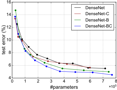
Figure 4: Left: Comparison of the parameter efficiency on C10+ between DenseNet variations. Middle: Comparison of the parameter efficiency between DenseNet-BC and (pre-activation) ResNets. DenseNet-BC requires about 1/3 of the parameters as ResNet to achieve comparable accuracy. Right: Training and testing curves of the 1001-layer pre-activation ResNet [12] with more than 10M parameters and a 100-layer DenseNet with only 0.8M parameters.

图 4：*左：*在 C10+ 上比较 DenseNet 各变体的参数效率。*中：*比较 DenseNet-BC 与（预激活）ResNet 的参数效率。要达到相当的精度，DenseNet-BC 所需参数约为 ResNet 的 1/3。*右：*参数量超过 10M 的 1001 层预激活 ResNet [12] 与参数仅 0.8M 的 100 层 DenseNet 的训练和测试曲线。

4.4 Classification Results on ImageNet

4.4 ImageNet 上的分类结果

We evaluate DenseNet-BC with different depths and growth rates on the ImageNet classification task, and compare it with state-of-the-art ResNet architectures. To ensure a fair comparison between the two architectures, we eliminate all other factors such as differences in data preprocessing and optimization settings by adopting the publicly available Torch implementation for ResNet by [8]¹. We simply replace the ResNet model with the DenseNet-BC network, and keep all the experiment settings exactly the same as those used for ResNet.

我们在 ImageNet 分类任务上评估不同深度和增长率的 DenseNet-BC，并与最先进的 ResNet 架构比较。为了保证两种架构的比较公平，我们直接采用 [8] 公开的 ResNet Torch 实现¹，排除数据预处理、优化设置等其他所有因素的差异。我们只是把 ResNet 模型换成 DenseNet-BC 网络，所有实验设置都与 ResNet 所用的完全相同。

¹ https://github.com/facebook/fb.resnet.torch

We report the single-crop and 10-crop validation errors of DenseNets on ImageNet in Table 3. Figure 3 shows the single-crop top-1 validation errors of DenseNets and ResNets as a function of the number of parameters (left) and FLOPs (right). The results presented in the figure reveal that DenseNets perform on par with the state-of-the-art ResNets, whilst requiring significantly fewer parameters and computation to achieve comparable performance. For example, a DenseNet-201 with 20M parameters model yields similar validation error as a 101-layer ResNet with more than 40M parameters. Similar trends can be observed from the right panel, which plots the validation error as a function of the number of FLOPs: a DenseNet that requires as much computation as a ResNet-50 performs on par with a ResNet-101, which requires twice as much computation.

表 3 报告了 DenseNet 在 ImageNet 上的单裁剪和 10 裁剪验证误差。图 3 给出了 DenseNet 和 ResNet 的单裁剪 top-1 验证误差随参数量（左）和 FLOPs（右）的变化。图中结果显示，DenseNet 与最先进的 ResNet 表现相当，而达到相当性能所需的参数和计算量明显更少。例如，参数量 20M 的 DenseNet-201 与参数量超过 40M 的 101 层 ResNet 验证误差相近。右图以 FLOPs 为横轴画出验证误差，也能看到类似趋势：计算量与 ResNet-50 相当的 DenseNet，表现与计算量是其两倍的 ResNet-101 相当。

It is worth noting that our experimental setup implies that we use hyperparameter settings that are optimized for ResNets but not for DenseNets. It is conceivable that more extensive hyper-parameter searches may further improve the performance of DenseNet on ImageNet.

需要说明的是，我们的实验设置意味着所用的超参数是为 ResNet 而不是为 DenseNet 优化的。可以设想，更充分的超参数搜索可能会进一步提升 DenseNet 在 ImageNet 上的性能。

5 Discussion

5 讨论

Superficially, DenseNets are quite similar to ResNets: Eq. (2) differs from Eq. (1) only in that the inputs to $H_{\ell}(\cdot)$ are concatenated instead of summed. However, the implications of this seemingly small modification lead to substantially different behaviors of the two network architectures.

表面上看，DenseNet 与 ResNet 十分相似：式 (2) 与式 (1) 的唯一区别是，$H_{\ell}(\cdot)$ 的输入是拼接而不是相加。然而，这一看似微小的修改，让两种网络架构的行为大不相同。

Model compactness.

As a direct consequence of the input concatenation, the feature-maps learned by any of the DenseNet layers can be accessed by all subsequent layers. This encourages feature reuse throughout the network, and leads to more compact models.

模型紧凑性。

输入拼接的直接结果是，DenseNet 任何一层学到的特征图都能被之后所有层访问。这鼓励了整个网络中的特征复用，使模型更紧凑。

The left two plots in Figure 4 show the result of an experiment that aims to compare the parameter efficiency of all variants of DenseNets (left) and also a comparable ResNet architecture (middle). We train multiple small networks with varying depths on C10+ and plot their test accuracies as a function of network parameters. In comparison with other popular network architectures, such as AlexNet [16] or VGG-net [29], ResNets with pre-activation use fewer parameters while typically achieving better results [12]. Hence, we compare DenseNet ($k=12$) against this architecture. The training setting for DenseNet is kept the same as in the previous section.

图 4 左边两幅图展示了一项实验的结果，用来比较 DenseNet 各变体（左）以及一个可比的 ResNet 架构（中）的参数效率。我们在 C10+ 上训练多个不同深度的小网络，并画出测试精度随网络参数量的变化。与 AlexNet [16]、VGG-net [29] 等其他流行网络架构相比，预激活 ResNet 使用的参数更少，结果通常却更好 [12]。因此我们拿 DenseNet（$k=12$）与这一架构比较。DenseNet 的训练设置与上一节相同。

The graph shows that DenseNet-BC is consistently the most parameter efficient variant of DenseNet. Further, to achieve the same level of accuracy, DenseNet-BC only requires around 1/3 of the parameters of ResNets (middle plot). This result is in line with the results on ImageNet we presented in Figure 3. The right plot in Figure 4 shows that a DenseNet-BC with only 0.8M trainable parameters is able to achieve comparable accuracy as the 1001-layer (pre-activation) ResNet [12] with 10.2M parameters.

图中显示，DenseNet-BC 一直是参数效率最高的 DenseNet 变体。此外，要达到同样的精度，DenseNet-BC 只需 ResNet 约 1/3 的参数（中图）。这与我们在图 3 中给出的 ImageNet 结果一致。图 4 右图显示，只有 0.8M 可训练参数的 DenseNet-BC，就能达到与 10.2M 参数的 1001 层（预激活）ResNet [12] 相当的精度。

Implicit Deep Supervision.

One explanation for the improved accuracy of dense convolutional networks may be that individual layers receive additional supervision from the loss function through the shorter connections. One can interpret DenseNets to perform a kind of “deep supervision”. The benefits of deep supervision have previously been shown in deeply-supervised nets (DSN; [20]), which have classifiers attached to every hidden layer, enforcing the intermediate layers to learn discriminative features.

隐式深度监督。

密集卷积网络精度更高的一个可能解释是，各层通过更短的连接从损失函数获得了额外的监督。可以把 DenseNet 理解为在做一种“深度监督”。深度监督的好处此前已在深度监督网络（DSN；[20]）中得到证明：DSN 在每个隐藏层上都接一个分类器，迫使中间层学习有判别力的特征。

DenseNets perform a similar deep supervision in an implicit fashion: a single classifier on top of the network provides direct supervision to all layers through at most two or three transition layers. However, the loss function and gradient of DenseNets are substantially less complicated, as the same loss function is shared between all layers.

DenseNet 以隐式方式实现了类似的深度监督：网络顶端的单个分类器最多经过两三个过渡层，就能对所有层提供直接监督。而且由于所有层共用同一个损失函数，DenseNet 的损失函数和梯度要简单得多。

Stochastic vs. deterministic connection.

There is an interesting connection between dense convolutional networks and stochastic depth regularization of residual networks [13]. In stochastic depth, layers in residual networks are randomly dropped, which creates direct connections between the surrounding layers. As the pooling layers are never dropped, the network results in a similar connectivity pattern as DenseNet: there is a small probability for any two layers, between the same pooling layers, to be directly connected—if all intermediate layers are randomly dropped. Although the methods are ultimately quite different, the DenseNet interpretation of stochastic depth may provide insights into the success of this regularizer.

随机连接与确定性连接。

密集卷积网络与残差网络的随机深度正则化 [13] 之间有一个有趣的联系。在随机深度中，残差网络的层被随机丢弃，从而在相邻的层之间建立直接连接。由于池化层从不被丢弃，网络形成了与 DenseNet 类似的连接模式：同一对池化层之间的任意两层，只要所有中间层都被随机丢弃，就有很小的概率直接相连。两种方法最终差别很大，但从 DenseNet 的角度理解随机深度，或许能帮助解释这一正则化方法为何有效。

Feature Reuse.

By design, DenseNets allow layers access to feature-maps from all of its preceding layers (although sometimes through transition layers). We conduct an experiment to investigate if a trained network takes advantage of this opportunity. We first train a DenseNet on C10+ with $L\!=\!40$ and $k\!=\!12$. For each convolutional layer $\ell$ within a block, we compute the average (absolute) weight assigned to connections with layer $s$. Figure 5 shows a heat-map for all three dense blocks. The average absolute weight serves as a surrogate for the dependency of a convolutional layer on its preceding layers. A red dot in position ($\ell,s$) indicates that the layer $\ell$ makes, on average, strong use of feature-maps produced $s$-layers before. Several observations can be made from the plot:

特征复用。

按设计，DenseNet 允许每一层访问之前所有层的特征图（有时要经过过渡层）。我们做了一个实验，考察训练好的网络是否真的利用了这一点。我们先在 C10+ 上训练一个 $L\!=\!40$、$k\!=\!12$ 的 DenseNet。对块内的每个卷积层 $\ell$，我们计算它与第 $s$ 层之间连接的平均（绝对）权重。图 5 给出了全部三个稠密块的热力图。平均绝对权重可以作为卷积层对之前各层依赖程度的替代指标。位置 ($\ell,s$) 处的红点表示第 $\ell$ 层平均而言大量使用了 $s$ 层之前产生的特征图。从图中可以得出几点观察：

1. All layers spread their weights over many inputs within the same block. This indicates that features extracted by very early layers are, indeed, directly used by deep layers throughout the same dense block.
2. The weights of the transition layers also spread their weight across all layers within the preceding dense block, indicating information flow from the first to the last layers of the DenseNet through few indirections.
3. The layers within the second and third dense block consistently assign the least weight to the outputs of the transition layer (the top row of the triangles), indicating that the transition layer outputs many redundant features (with low weight on average). This is in keeping with the strong results of DenseNet-BC where exactly these outputs are compressed.
4. Although the final classification layer, shown on the very right, also uses weights across the entire dense block, there seems to be a concentration towards final feature-maps, suggesting that there may be some more high-level features produced late in the network.

1. 所有层都把权重分散在同一块内的许多输入上。这说明很早的层提取的特征，确实被同一稠密块中很深的层直接使用。
2. 过渡层的权重也分散在前一个稠密块的所有层上，说明信息只需经过很少的间接环节，就能从 DenseNet 的最前几层流到最后几层。
3. 第二和第三个稠密块中的层，一致地给过渡层的输出（三角形的最上面一行）分配最小的权重，说明过渡层输出了许多冗余特征（平均权重较低）。这与 DenseNet-BC 的强劲结果相吻合，因为 DenseNet-BC 压缩的正是这些输出。
4. 最右侧所示的最终分类层也使用了整个稠密块上的权重，但看起来更集中于最后的特征图，说明网络后段可能产生了更多高层特征。

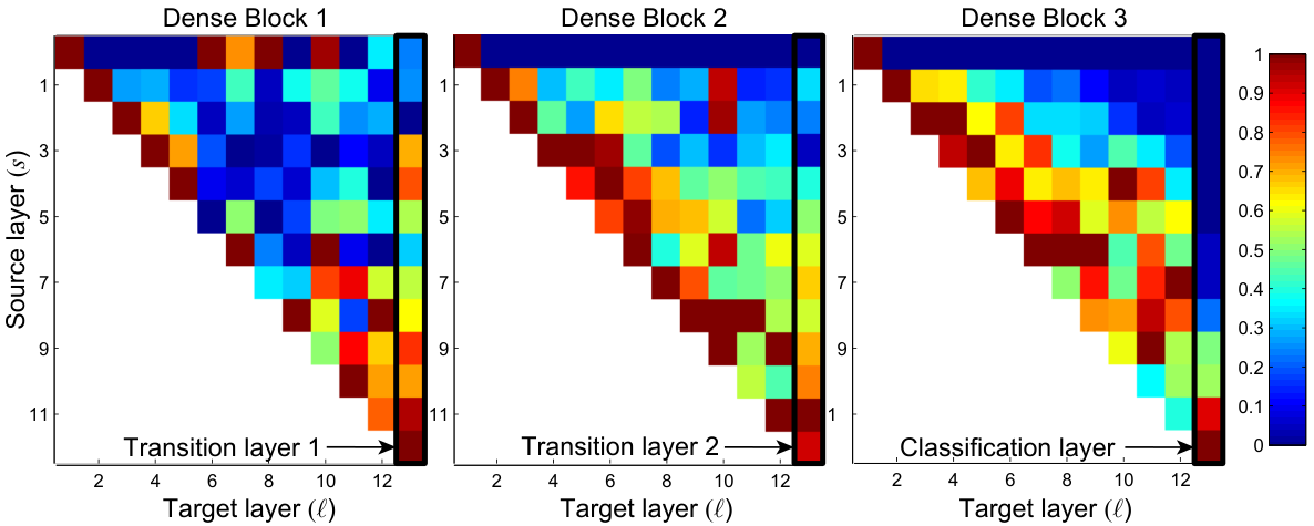
Figure 5: The average absolute filter weights of convolutional layers in a trained DenseNet. The color of pixel $(s,\ell)$ encodes the average $L1$ norm (normalized by number of input feature-maps) of the weights connecting convolutional layer $s$ to $\ell$ within a dense block. Three columns highlighted by black rectangles correspond to two transition layers and the classification layer. The first row encodes weights connected to the input layer of the dense block.

图 5：一个训练好的 DenseNet 中卷积层的平均绝对滤波器权重。像素 $(s,\ell)$ 的颜色表示在一个稠密块内连接卷积层 $s$ 与 $\ell$ 的权重的平均 $L1$ 范数（按输入特征图数量归一化）。黑色矩形框出的三列分别对应两个过渡层和分类层。第一行表示与稠密块输入层相连的权重。

6 Conclusion

6 结论

We proposed a new convolutional network architecture, which we refer to as Dense Convolutional Network (DenseNet). It introduces direct connections between any two layers with the same feature-map size. We showed that DenseNets scale naturally to hundreds of layers, while exhibiting no optimization difficulties. In our experiments, DenseNets tend to yield consistent improvement in accuracy with growing number of parameters, without any signs of performance degradation or overfitting. Under multiple settings, it achieved state-of-the-art results across several highly competitive datasets. Moreover, DenseNets require substantially fewer parameters and less computation to achieve state-of-the-art performances. Because we adopted hyperparameter settings optimized for residual networks in our study, we believe that further gains in accuracy of DenseNets may be obtained by more detailed tuning of hyperparameters and learning rate schedules.

我们提出了一种新的卷积网络架构，称为密集卷积网络（DenseNet）。它在任意两个特征图尺寸相同的层之间建立直接连接。我们表明，DenseNet 可以自然地扩展到数百层，而不出现优化困难。实验中，随着参数量增加，DenseNet 的精度往往稳定提升，没有任何性能退化或过拟合的迹象。在多种设置下，它在若干竞争激烈的数据集上取得了最先进的结果。此外，DenseNet 达到最先进性能所需的参数和计算量都少得多。由于本研究采用的是为残差网络优化的超参数设置，我们相信，对超参数和学习率调度做更细致的调整，可能会让 DenseNet 的精度进一步提高。

Whilst following a simple connectivity rule, DenseNets naturally integrate the properties of identity mappings, deep supervision, and diversified depth. They allow feature reuse throughout the networks and can consequently learn more compact and, according to our experiments, more accurate models. Because of their compact internal representations and reduced feature redundancy, DenseNets may be good feature extractors for various computer vision tasks that build on convolutional features, e.g.,  [4, 5]. We plan to study such feature transfer with DenseNets in future work.

DenseNet 遵循一条简单的连接规则，却自然地融合了恒等映射、深度监督和多样化深度的特性。它允许在整个网络中复用特征，因而能学到更紧凑的模型，而且根据我们的实验，也更准确。由于内部表征紧凑、特征冗余较少，DenseNet 可能是各种基于卷积特征的计算机视觉任务（例如 [4, 5]）的良好特征提取器。我们计划在未来的工作中研究 DenseNet 的这种特征迁移。

Acknowledgements.

The authors are supported in part by the NSF III-1618134, III-1526012, IIS-1149882, the Office of Naval Research Grant N00014-17-1-2175 and the Bill and Melinda Gates foundation. GH is supported by the International Postdoctoral Exchange Fellowship Program of China Postdoctoral Council (No.20150015). ZL is supported by the National Basic Research Program of China Grants 2011CBA00300, 2011CBA00301, the NSFC 61361136003. We also thank Daniel Sedra, Geoff Pleiss and Yu Sun for many insightful discussions.

致谢。

作者部分受到 NSF III-1618134、III-1526012、IIS-1149882，美国海军研究办公室（Office of Naval Research）资助 N00014-17-1-2175，以及比尔及梅琳达·盖茨基金会的支持。黄高受中国博士后科学基金会博士后国际交流计划（编号 20150015）资助。刘壮受国家重点基础研究发展计划资助 2011CBA00300、2011CBA00301 以及国家自然科学基金 61361136003 资助。我们还感谢 Daniel Sedra、Geoff Pleiss 和 Yu Sun 的许多富有启发的讨论。

References

参考文献

[1] C. Cortes, X. Gonzalvo, V. Kuznetsov, M. Mohri, and S. Yang. Adanet: Adaptive structural learning of artificial neural networks. arXiv preprint arXiv:1607.01097, 2016.

[2] J. Deng, W. Dong, R. Socher, L.-J. Li, K. Li, and L. Fei-Fei. Imagenet: A large-scale hierarchical image database. In CVPR, 2009.

[3] S. E. Fahlman and C. Lebiere. The cascade-correlation learning architecture. In NIPS, 1989.

[4] J. R. Gardner, M. J. Kusner, Y. Li, P. Upchurch, K. Q. Weinberger, and J. E. Hopcroft. Deep manifold traversal: Changing labels with convolutional features. arXiv preprint arXiv:1511.06421, 2015.

[5] L. Gatys, A. Ecker, and M. Bethge. A neural algorithm of artistic style. Nature Communications, 2015.

[6] X. Glorot, A. Bordes, and Y. Bengio. Deep sparse rectifier neural networks. In AISTATS, 2011.

[7] I. Goodfellow, D. Warde-Farley, M. Mirza, A. Courville, and Y. Bengio. Maxout networks. In ICML, 2013.

[8] S. Gross and M. Wilber. Training and investigating residual nets, 2016.

[9] B. Hariharan, P. Arbeláez, R. Girshick, and J. Malik. Hypercolumns for object segmentation and fine-grained localization. In CVPR, 2015.

[10] K. He, X. Zhang, S. Ren, and J. Sun. Delving deep into rectifiers: Surpassing human-level performance on imagenet classification. In ICCV, 2015.

[11] K. He, X. Zhang, S. Ren, and J. Sun. Deep residual learning for image recognition. In CVPR, 2016.

[12] K. He, X. Zhang, S. Ren, and J. Sun. Identity mappings in deep residual networks. In ECCV, 2016.

[13] G. Huang, Y. Sun, Z. Liu, D. Sedra, and K. Q. Weinberger. Deep networks with stochastic depth. In ECCV, 2016.

[14] S. Ioffe and C. Szegedy. Batch normalization: Accelerating deep network training by reducing internal covariate shift. In ICML, 2015.

[15] A. Krizhevsky and G. Hinton. Learning multiple layers of features from tiny images. Tech Report, 2009.

[16] A. Krizhevsky, I. Sutskever, and G. E. Hinton. Imagenet classification with deep convolutional neural networks. In NIPS, 2012.

[17] G. Larsson, M. Maire, and G. Shakhnarovich. Fractalnet: Ultra-deep neural networks without residuals. arXiv preprint arXiv:1605.07648, 2016.

[18] Y. LeCun, B. Boser, J. S. Denker, D. Henderson, R. E. Howard, W. Hubbard, and L. D. Jackel. Backpropagation applied to handwritten zip code recognition. Neural computation, 1(4):541–551, 1989.

[19] Y. LeCun, L. Bottou, Y. Bengio, and P. Haffner. Gradient-based learning applied to document recognition. Proceedings of the IEEE, 86(11):2278–2324, 1998.

[20] C.-Y. Lee, S. Xie, P. Gallagher, Z. Zhang, and Z. Tu. Deeply-supervised nets. In AISTATS, 2015.

[21] Q. Liao and T. Poggio. Bridging the gaps between residual learning, recurrent neural networks and visual cortex. arXiv preprint arXiv:1604.03640, 2016.

[22] M. Lin, Q. Chen, and S. Yan. Network in network. In ICLR, 2014.

[23] J. Long, E. Shelhamer, and T. Darrell. Fully convolutional networks for semantic segmentation. In CVPR, 2015.

[24] Y. Netzer, T. Wang, A. Coates, A. Bissacco, B. Wu, and A. Y. Ng. Reading digits in natural images with unsupervised feature learning, 2011. In NIPS Workshop, 2011.

[25] M. Pezeshki, L. Fan, P. Brakel, A. Courville, and Y. Bengio. Deconstructing the ladder network architecture. In ICML, 2016.

[26] G. Pleiss, D. Chen, G. Huang, T. Li, L. van der Maaten, and K. Q. Weinberger. Memory-efficient implementation of densenets. arXiv preprint arXiv:1707.06990, 2017.

[27] A. Rasmus, M. Berglund, M. Honkala, H. Valpola, and T. Raiko. Semi-supervised learning with ladder networks. In NIPS, 2015.

[28] A. Romero, N. Ballas, S. E. Kahou, A. Chassang, C. Gatta, and Y. Bengio. Fitnets: Hints for thin deep nets. In ICLR, 2015.

[29] O. Russakovsky, J. Deng, H. Su, J. Krause, S. Satheesh, S. Ma, Z. Huang, A. Karpathy, A. Khosla, M. Bernstein, et al. Imagenet large scale visual recognition challenge. IJCV.

[30] P. Sermanet, S. Chintala, and Y. LeCun. Convolutional neural networks applied to house numbers digit classification. In ICPR, pages 3288–3291. IEEE, 2012.

[31] P. Sermanet, K. Kavukcuoglu, S. Chintala, and Y. LeCun. Pedestrian detection with unsupervised multi-stage feature learning. In CVPR, 2013.

[32] J. T. Springenberg, A. Dosovitskiy, T. Brox, and M. Riedmiller. Striving for simplicity: The all convolutional net. arXiv preprint arXiv:1412.6806, 2014.

[33] N. Srivastava, G. E. Hinton, A. Krizhevsky, I. Sutskever, and R. Salakhutdinov. Dropout: a simple way to prevent neural networks from overfitting. JMLR, 2014.

[34] R. K. Srivastava, K. Greff, and J. Schmidhuber. Training very deep networks. In NIPS, 2015.

[35] I. Sutskever, J. Martens, G. Dahl, and G. Hinton. On the importance of initialization and momentum in deep learning. In ICML, 2013.

[36] C. Szegedy, W. Liu, Y. Jia, P. Sermanet, S. Reed, D. Anguelov, D. Erhan, V. Vanhoucke, and A. Rabinovich. Going deeper with convolutions. In CVPR, 2015.

[37] C. Szegedy, V. Vanhoucke, S. Ioffe, J. Shlens, and Z. Wojna. Rethinking the inception architecture for computer vision. In CVPR, 2016.

[38] S. Targ, D. Almeida, and K. Lyman. Resnet in resnet: Generalizing residual architectures. arXiv preprint arXiv:1603.08029, 2016.

[39] J. Wang, Z. Wei, T. Zhang, and W. Zeng. Deeply-fused nets. arXiv preprint arXiv:1605.07716, 2016.

[40] B. M. Wilamowski and H. Yu. Neural network learning without backpropagation. IEEE Transactions on Neural Networks, 21(11):1793–1803, 2010.

[41] S. Yang and D. Ramanan. Multi-scale recognition with dag-cnns. In ICCV, 2015.

[42] S. Zagoruyko and N. Komodakis. Wide residual networks. arXiv preprint arXiv:1605.07146, 2016.

[43] Y. Zhang, K. Lee, and H. Lee. Augmenting supervised neural networks with unsupervised objectives for large-scale image classification. In ICML, 2016.