Delving Deep into Rectifiers: Surpassing Human-Level Performance on ImageNet Classification

Kaiming He    Xiangyu Zhang    Shaoqing Ren    Jian Sun Affiliation: Microsoft Research Email: {kahe,˜v-xiangz,˜v-shren,˜jiansun}@microsoft.com

Abstract

摘要

Rectified activation units (rectifiers) are essential for state-of-the-art neural networks. In this work, we study rectifier neural networks for image classification from two aspects. First, we propose a Parametric Rectified Linear Unit (PReLU) that generalizes the traditional rectified unit. PReLU improves model fitting with nearly zero extra computational cost and little overfitting risk. Second, we derive a robust initialization method that particularly considers the rectifier nonlinearities. This method enables us to train extremely deep rectified models directly from scratch and to investigate deeper or wider network architectures. Based on our PReLU networks (PReLU-nets), we achieve 4.94% top-5 test error on the ImageNet 2012 classification dataset. This is a 26% relative improvement over the ILSVRC 2014 winner (GoogLeNet, 6.66% [29]). To our knowledge, our result is the first to surpass human-level performance (5.1%, [22]) on this visual recognition challenge.

整流激活单元（rectifier）对当时最好的神经网络至关重要。本文从两个方面研究用于图像分类的整流神经网络。第一，我们提出参数化整流线性单元（Parametric Rectified Linear Unit，PReLU），它是对传统整流单元的推广。PReLU 以几乎为零的额外计算代价改进模型拟合，并且几乎不增加过拟合风险。第二，我们推导一种特别考虑整流非线性的稳健初始化方法。这一方法使我们能够从零直接训练极深的整流模型，并探索更深或更宽的网络结构。基于我们的 PReLU 网络（PReLU-nets），我们在 ImageNet 2012 分类数据集上达到 4.94% 的 top-5 测试误差。这相对 ILSVRC 2014 获胜者（GoogLeNet，6.66% [29]）有 26% 的相对提升。据我们所知，这一结果首次在该视觉识别挑战上超过了人类水平的表现（5.1%，[22]）。

1 Introduction

1 引言

Convolutional neural networks (CNNs) [17, 16] have demonstrated recognition accuracy better than or comparable to humans in several visual recognition tasks, including recognizing traffic signs [3], faces [30, 28], and hand-written digits [3, 31]. In this work, we present a result that surpasses human-level performance on a more generic and challenging recognition task - the classification task in the 1000-class ImageNet dataset [22].

卷积神经网络（CNN）[17, 16] 已在若干视觉识别任务上展示出优于或相当于人类的识别精度，包括识别交通标志 [3]、人脸 [30, 28] 和手写数字 [3, 31]。在本工作中，我们在一项更通用、也更具挑战性的识别任务上给出超过人类水平的结果——1000 类 ImageNet 数据集 [22] 上的分类任务。

In the last few years, we have witnessed tremendous improvements in recognition performance, mainly due to advances in two technical directions: building more powerful models, and designing effective strategies against overfitting. On one hand, neural networks are becoming more capable of fitting training data, because of increased complexity (e.g., increased depth [25, 29], enlarged width [33, 24], and the use of smaller strides [33, 24, 2, 25]), new nonlinear activations [21, 20, 34, 19, 27, 9], and sophisticated layer designs [29, 11]. On the other hand, better generalization is achieved by effective regularization techniques [12, 26, 9, 31], aggressive data augmentation [16, 13, 25, 29], and large-scale data [4, 22].

过去几年，识别性能出现了巨大提升，主要得益于两个技术方向的进展：构建更强的模型，以及设计有效的策略来抑制过拟合。一方面，神经网络拟合训练数据的能力越来越强，原因包括复杂度增加（例如加深 [25, 29]、加宽 [33, 24]，以及使用更小的步长 [33, 24, 2, 25]）、新的非线性激活 [21, 20, 34, 19, 27, 9]，以及更精细的层设计 [29, 11]。另一方面，有效的正则化技术 [12, 26, 9, 31]、更强的数据增强 [16, 13, 25, 29] 以及大规模数据 [4, 22]，带来了更好的泛化。

Among these advances, the rectifier neuron [21, 8, 20, 34], e.g., Rectified Linear Unit (ReLU), is one of several keys to the recent success of deep networks [16]. It expedites convergence of the training procedure [16] and leads to better solutions [21, 8, 20, 34] than conventional sigmoid-like units. Despite the prevalence of rectifier networks, recent improvements of models [33, 24, 11, 25, 29] and theoretical guidelines for training them [7, 23] have rarely focused on the properties of the rectifiers.

在这些进展中，整流神经元 [21, 8, 20, 34]，例如整流线性单元（ReLU），是深度网络近期成功的几个关键之一 [16]。它加快训练过程的收敛 [16]，并且比传统的类 sigmoid 单元得到更好的解 [21, 8, 20, 34]。尽管整流网络已经普及，近期对模型的改进 [33, 24, 11, 25, 29] 以及训练它们的理论指南 [7, 23]，却很少把注意力放在整流器本身的性质上。

In this paper, we investigate neural networks from two aspects particularly driven by the rectifiers. First, we propose a new generalization of ReLU, which we call Parametric Rectified Linear Unit (PReLU). This activation function adaptively learns the parameters of the rectifiers, and improves accuracy at negligible extra computational cost. Second, we study the difficulty of training rectified models that are very deep. By explicitly modeling the nonlinearity of rectifiers (ReLU/PReLU), we derive a theoretically sound initialization method, which helps with convergence of very deep models (e.g., with 30 weight layers) trained directly from scratch. This gives us more flexibility to explore more powerful network architectures.

本文从由整流器特别驱动的两个方面研究神经网络。第一，我们提出对 ReLU 的一种新推广，称为参数化整流线性单元（PReLU）。这一激活函数自适应地学习整流器的参数，并以几乎可以忽略的额外计算代价提升精度。第二，我们研究训练非常深的整流模型的困难。通过显式建模整流器（ReLU/PReLU）的非线性，我们推导出一种理论上合理的初始化方法，有助于极深模型（例如 30 个权重层）从零直接训练时收敛。这使我们有更大的灵活性去探索更强的网络结构。

On the 1000-class ImageNet 2012 dataset, our PReLU network (PReLU-net) leads to a single-model result of 5.71% top-5 error, which surpasses all existing multi-model results. Further, our multi-model result achieves 4.94% top-5 error on the test set, which is a 26% relative improvement over the ILSVRC 2014 winner (GoogLeNet, 6.66% [29]). To the best of our knowledge, our result surpasses for the first time the reported human-level performance (5.1% in [22]) on this visual recognition challenge.

在 1000 类 ImageNet 2012 数据集上，我们的 PReLU 网络（PReLU-net）给出 5.71% top-5 误差的单模型结果，超过了当时所有已有的多模型结果。进一步地，我们的多模型结果在测试集上达到 4.94% 的 top-5 误差，相对 ILSVRC 2014 获胜者（GoogLeNet，6.66% [29]）有 26% 的相对提升。据我们所知，这一结果首次超过了该视觉识别挑战中报告的人类水平表现（[22] 中的 5.1%）。

2 Approach

2 方法

In this section, we first present the PReLU activation function (Sec. 2.1). Then we derive our initialization method for deep rectifier networks (Sec. 2.2). Lastly we discuss our architecture designs (Sec. 2.3).

本节我们首先介绍 PReLU 激活函数（第 2.1 节）。然后推导面向深度整流网络的初始化方法（第 2.2 节）。最后讨论我们的结构设计（第 2.3 节）。

2.1 Parametric Rectifiers

2.1 参数化整流器

We show that replacing the parameter-free ReLU activation by a learned parametric activation unit improves classification accuracy[^1].

[^1]: Concurrent with our work, Agostinelli et al. [1] also investigated learning activation functions and showed improvement on other tasks.

我们表明，用可学习的参数化激活单元替换无参数的 ReLU 激活，能够提升分类精度。[^1]

[^1]: 与我们同期，Agostinelli 等人 [1] 也研究了学习激活函数，并在其他任务上展示了改进。

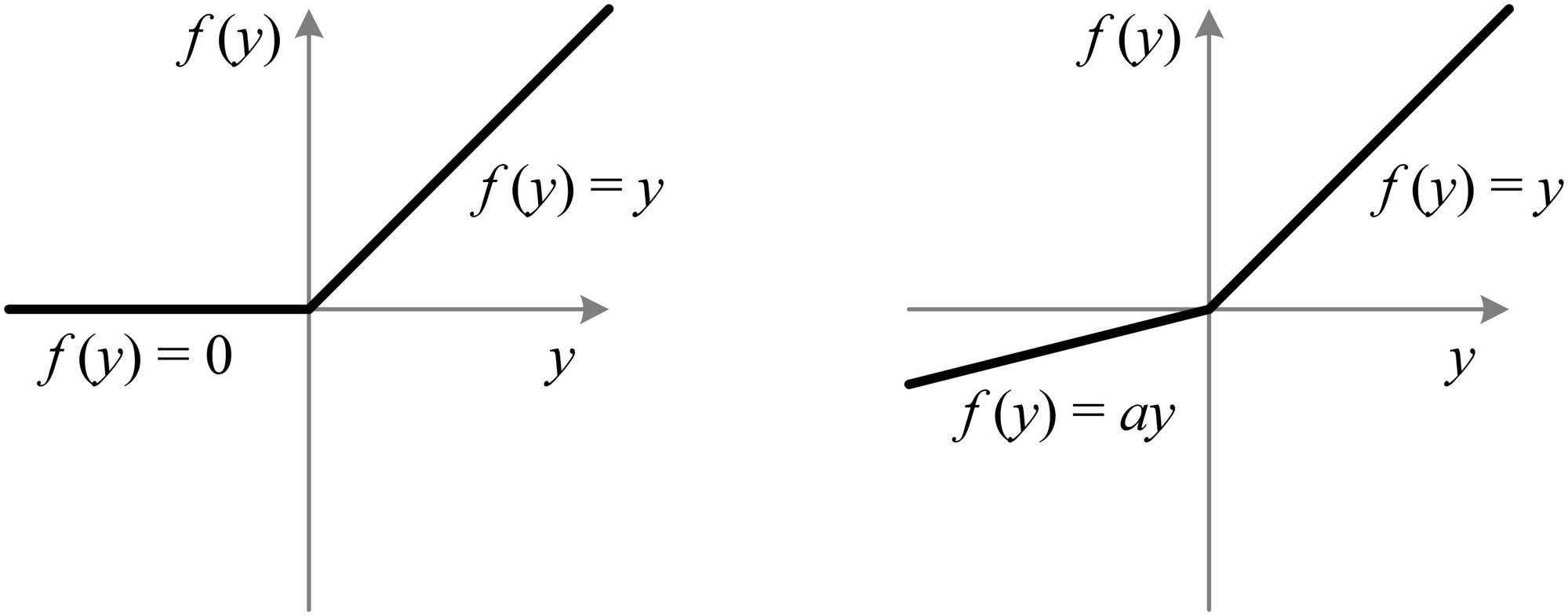
Figure 1: ReLU vs. PReLU. For PReLU, the coefficient of the negative part is not constant and is adaptively learned.

图 1：ReLU 与 PReLU。对 PReLU 而言，负半轴的系数不是常数，而是自适应学习得到的。

Definition

Formally, we consider an activation function defined as:

定义

形式上，我们考虑如下定义的激活函数：

$$f(y_{i})=\begin{cases}y_{i},&\mbox{if }y_{i}>0\
a_{i}y_{i},&\mbox{if }y_{i}\leq 0\end{cases}. \tag{1}$$

Here $y_{i}$ is the input of the nonlinear activation $f$ on the $i$th channel, and $a_{i}$ is a coefficient controlling the slope of the negative part. The subscript $i$ in $a_{i}$ indicates that we allow the nonlinear activation to vary on different channels. When $a_{i}=0$, it becomes ReLU; when $a_{i}$ is a learnable parameter, we refer to Eqn.(1) as Parametric ReLU (PReLU). Figure 1 shows the shapes of ReLU and PReLU. Eqn.(1) is equivalent to $f(y_{i})=\max(0,y_{i})+a_{i}\min(0,y_{i})$.

这里 $y_{i}$ 是第 $i$ 个通道上非线性激活 $f$ 的输入，$a_{i}$ 是控制负半轴斜率的系数。$a_{i}$ 中的下标 $i$ 表示我们允许非线性激活在不同通道上有所不同。当 $a_{i}=0$ 时，它就是 ReLU；当 $a_{i}$ 是可学习参数时，我们把式（1）称为参数化 ReLU（PReLU）。图 1 给出了 ReLU 和 PReLU 的形状。式（1）等价于 $f(y_{i})=\max(0,y_{i})+a_{i}\min(0,y_{i})$。

If $a_{i}$ is a small and fixed value, PReLU becomes the Leaky ReLU (LReLU) in [20] ($a_{i}=0.01$). The motivation of LReLU is to avoid zero gradients. Experiments in [20] show that LReLU has negligible impact on accuracy compared with ReLU. On the contrary, our method adaptively learns the PReLU parameters jointly with the whole model. We hope for end-to-end training that will lead to more specialized activations.

如果 $a_{i}$ 是一个较小的固定值，PReLU 就变成 [20] 中的 Leaky ReLU（LReLU）（$a_{i}=0.01$）。LReLU 的动机是避免零梯度。[20] 中的实验表明，与 ReLU 相比，LReLU 对精度的影响可以忽略。与之相反，我们的方法与整个模型一起自适应地学习 PReLU 参数。我们希望端到端训练能得到更专门化的激活。

PReLU introduces a very small number of extra parameters. The number of extra parameters is equal to the total number of channels, which is negligible when considering the total number of weights. So we expect no extra risk of overfitting. We also consider a channel-shared variant: $f(y_{i})=\max(0,y_{i})+a\min(0,y_{i})$ where the coefficient is shared by all channels of one layer. This variant only introduces a single extra parameter into each layer.

PReLU 只引入非常少的额外参数。额外参数的数目等于通道总数，相对权重总数可以忽略。因此我们预期不会增加额外的过拟合风险。我们还考虑一种通道共享的变体：$f(y_{i})=\max(0,y_{i})+a\min(0,y_{i})$，其中系数在一层的所有通道上共享。这一变体在每一层只引入一个额外参数。

Optimization

PReLU can be trained using backpropagation [17] and optimized simultaneously with other layers. The update formulations of $\{a_{i}\}$ are simply derived from the chain rule. The gradient of $a_{i}$ for one layer is:

优化

PReLU 可以用反向传播 [17] 训练，并与其他层同时优化。$\{a_{i}\}$ 的更新公式由链式法则直接推出。一层中 $a_{i}$ 的梯度为：

$$\frac{\partial\mathcal{E}}{\partial a_{i}}=\sum_{y_{i}}\frac{\partial\mathcal{E}}{\partial f(y_{i})}\frac{\partial f(y_{i})}{\partial a_{i}}, \tag{2}$$

where $\mathcal{E}$ represents the objective function. The term $\frac{\partial\mathcal{E}}{\partial f(y_{i})}$ is the gradient propagated from the deeper layer. The gradient of the activation is given by:

其中 $\mathcal{E}$ 表示目标函数。项 $\frac{\partial\mathcal{E}}{\partial f(y_{i})}$ 是从更深一层传回来的梯度。激活函数的梯度由下式给出：

$$\frac{\partial f(y_{i})}{\partial a_{i}}=\begin{cases}0,&\mbox{if }y_{i}>0\
y_{i},&\mbox{if }y_{i}\leq 0\end{cases}. \tag{3}$$

The summation $\sum_{y_{i}}$ runs over all positions of the feature map. For the channel-shared variant, the gradient of $a$ is $\frac{\partial\mathcal{E}}{\partial a}=\sum_{i}\sum_{y_{i}}\frac{\partial\mathcal{E}}{\partial f(y_{i})}\frac{\partial f(y_{i})}{\partial a}$, where $\sum_{i}$ sums over all channels of the layer. The time complexity due to PReLU is negligible for both forward and backward propagation.

求和 $\sum_{y_{i}}$ 遍历特征图上的所有位置。对通道共享的变体，$a$ 的梯度为 $\frac{\partial\mathcal{E}}{\partial a}=\sum_{i}\sum_{y_{i}}\frac{\partial\mathcal{E}}{\partial f(y_{i})}\frac{\partial f(y_{i})}{\partial a}$，其中 $\sum_{i}$ 对该层所有通道求和。无论前向还是反向传播，PReLU 带来的时间复杂度都可以忽略。

We adopt the momentum method when updating $a_{i}$:

更新 $a_{i}$ 时我们采用动量法：

$$\Delta a_{i}:=\mu\Delta a_{i}+\epsilon\frac{\partial\mathcal{E}}{\partial a_{i}}. \tag{4}$$

Here $\mu$ is the momentum and $\epsilon$ is the learning rate. It is worth noticing that we do not use weight decay ($l_{2}$ regularization) when updating $a_{i}$. A weight decay tends to push $a_{i}$ to zero, and thus biases PReLU toward ReLU. Even without regularization, the learned coefficients rarely have a magnitude larger than 1 in our experiments. Further, we do not constrain the range of $a_{i}$ so that the activation function may be non-monotonic. We use $a_{i}=0.25$ as the initialization throughout this paper.

这里 $\mu$ 是动量，$\epsilon$ 是学习率。值得注意的是，更新 $a_{i}$ 时我们不使用权重衰减（$l_{2}$ 正则）。权重衰减往往会把 $a_{i}$ 推向零，从而使 PReLU 偏向 ReLU。即使不加正则，实验中学到的系数幅值也很少大于 1。此外，我们不限制 $a_{i}$ 的取值范围，因此激活函数可以是非单调的。本文始终用 $a_{i}=0.25$ 作为初始化。

Comparison Experiments

We conducted comparisons on a deep but efficient model with 14 weight layers. The model was studied in [10] (model E of [10]) and its architecture is described in Table 1. We choose this model because it is sufficient for representing a category of very deep models, as well as to make the experiments feasible.

对比实验

我们在一个有 14 个权重层、既深又高效的模型上做了对比。该模型在 [10] 中研究过（[10] 的模型 E），结构见表 1。我们选择这一模型，是因为它足以代表一类很深的模型，同时也使实验可行。

As a baseline, we train this model with ReLU applied in the convolutional (conv) layers and the first two fully-connected (fc) layers. The training implementation follows [10]. The top-1 and top-5 errors are 33.82% and 13.34% on ImageNet 2012, using 10-view testing (Table 2).

作为基线，我们在卷积（conv）层和前两个全连接（fc）层上使用 ReLU 来训练这一模型。训练实现遵循 [10]。在 ImageNet 2012 上，用 10 视图测试得到的 top-1 和 top-5 误差为 33.82% 和 13.34%（表 2）。

	learned coefficients
layer	channel-shared	channel-wise
conv1	7$\times$7, 64, /2	0.681	0.596
pool1	3$\times$3, /3
conv21	2$\times$2, 128	0.103	0.321
conv22	2$\times$2, 128	0.099	0.204
conv23	2$\times$2, 128	0.228	0.294
conv24	2$\times$2, 128	0.561	0.464
pool2	2$\times$2, /2
conv31	2$\times$2, 256	0.126	0.196
conv32	2$\times$2, 256	0.089	0.152
conv33	2$\times$2, 256	0.124	0.145
conv34	2$\times$2, 256	0.062	0.124
conv35	2$\times$2, 256	0.008	0.134
conv36	2$\times$2, 256	0.210	0.198
spp	$\{6,3,2,1\}$
fc1	4096	0.063	0.074
fc2	4096	0.031	0.075
fc3	1000

Table 1: A small but deep 14-layer model [10]. The filter size and filter number of each layer is listed. The number /$s$ indicates the stride $s$ that is used. The learned coefficients of PReLU are also shown. For the channel-wise case, the average of $\{a_{i}\}$ over the channels is shown for each layer.

	学到的系数
层	通道共享	逐通道
conv1	7$\times$7, 64, /2	0.681	0.596
pool1	3$\times$3, /3
conv21	2$\times$2, 128	0.103	0.321
conv22	2$\times$2, 128	0.099	0.204
conv23	2$\times$2, 128	0.228	0.294
conv24	2$\times$2, 128	0.561	0.464
pool2	2$\times$2, /2
conv31	2$\times$2, 256	0.126	0.196
conv32	2$\times$2, 256	0.089	0.152
conv33	2$\times$2, 256	0.124	0.145
conv34	2$\times$2, 256	0.062	0.124
conv35	2$\times$2, 256	0.008	0.134
conv36	2$\times$2, 256	0.210	0.198
spp	$\{6,3,2,1\}$
fc1	4096	0.063	0.074
fc2	4096	0.031	0.075
fc3	1000

表 1：一个既小又深的 14 层模型 [10]。列出了每层的滤波器尺寸和滤波器数目。/$s$ 表示使用的步长 $s$。同时也给出了 PReLU 学到的系数。对逐通道情形，给出的是各层上 $\{a_{i}\}$ 在通道上的平均值。

Then we train the same architecture from scratch, with all ReLUs replaced by PReLUs (Table 2). The top-1 error is reduced to 32.64%. This is a 1.2% gain over the ReLU baseline. Table 2 also shows that channel-wise/channel-shared PReLUs perform comparably. For the channel-shared version, PReLU only introduces 13 extra free parameters compared with the ReLU counterpart. But this small number of free parameters play critical roles as evidenced by the 1.1% gain over the baseline. This implies the importance of adaptively learning the shapes of activation functions.

然后我们从零训练同一结构，把所有 ReLU 换成 PReLU（表 2）。top-1 误差降到 32.64%。这相对 ReLU 基线有 1.2 个百分点的提升。表 2 还显示，逐通道与通道共享的 PReLU 表现相当。对通道共享版本，与 ReLU 对照相比，PReLU 只引入 13 个额外自由参数。但这一小数量的自由参数起着关键作用，相对基线有 1.1 个百分点的提升。这意味着自适应学习激活函数形状很重要。

	top-1	top-5
ReLU	33.82	13.34
PReLU, channel-shared	32.71	12.87
PReLU, channel-wise	32.64	12.75

Table 2: Comparisons between ReLU and PReLU on the small model. The error rates are for ImageNet 2012 using 10-view testing. The images are resized so that the shorter side is 256, during both training and testing. Each view is 224$\times$224. All models are trained using 75 epochs.

	top-1	top-5
ReLU	33.82	13.34
PReLU，通道共享	32.71	12.87
PReLU，逐通道	32.64	12.75

表 2：小模型上 ReLU 与 PReLU 的比较。误差率针对 ImageNet 2012，采用 10 视图测试。训练和测试时都把图像缩放，使较短边为 256。每个视图为 224$\times$224。所有模型都训练 75 个周期。

Table 1 also shows the learned coefficients of PReLUs for each layer. There are two interesting phenomena in Table 1. First, the first conv layer (conv1) has coefficients (0.681 and 0.596) significantly greater than 0. As the filters of conv1 are mostly Gabor-like filters such as edge or texture detectors, the learned results show that both positive and negative responses of the filters are respected. We believe that this is a more economical way of exploiting low-level information, given the limited number of filters (e.g., 64). Second, for the channel-wise version, the deeper conv layers in general have smaller coefficients. This implies that the activations gradually become “more nonlinear” at increasing depths. In other words, the learned model tends to keep more information in earlier stages and becomes more discriminative in deeper stages.

表 1 还给出了各层 PReLU 学到的系数。表 1 中有两个有意思的现象。第一，第一个卷积层（conv1）的系数（0.681 和 0.596）明显大于 0。由于 conv1 的滤波器大多是类 Gabor 的边缘或纹理检测器，学习结果表明滤波器的正响应和负响应都被保留。我们认为，在滤波器数目有限时（例如 64 个），这是一种更经济地利用底层信息的方式。第二，对逐通道版本，更深的卷积层系数一般更小。这意味着随着深度增加，激活逐渐变得“更加非线性”。换句话说，学到的模型倾向于在较早阶段保留更多信息，而在更深阶段变得更有判别性。

2.2 Initialization of Filter Weights for Rectifiers

2.2 面向整流器的滤波器权重初始化

Rectifier networks are easier to train [8, 16, 34] compared with traditional sigmoid-like activation networks. But a bad initialization can still hamper the learning of a highly non-linear system. In this subsection, we propose a robust initialization method that removes an obstacle of training extremely deep rectifier networks.

与传统的类 sigmoid 激活网络相比，整流网络更容易训练 [8, 16, 34]。但糟糕的初始化仍然会妨碍高度非线性系统的学习。本小节我们提出一种稳健的初始化方法，以消除训练极深整流网络的一个障碍。

Recent deep CNNs are mostly initialized by random weights drawn from Gaussian distributions [16]. With fixed standard deviations (e.g., 0.01 in [16]), very deep models (e.g., $>$8 conv layers) have difficulties to converge, as reported by the VGG team [25] and also observed in our experiments. To address this issue, in [25] they pre-train a model with 8 conv layers to initialize deeper models. But this strategy requires more training time, and may also lead to a poorer local optimum. In [29, 18], auxiliary classifiers are added to intermediate layers to help with convergence.

近期的深层 CNN 大多用从高斯分布中抽取的随机权重来初始化 [16]。在标准差固定时（例如 [16] 中的 0.01），很深的模型（例如超过 8 个卷积层）很难收敛，这是 VGG 团队 [25] 报告过的，也在我们的实验中观察到。为解决这一问题，[25] 先预训练一个有 8 个卷积层的模型，再用来初始化更深的模型。但这一策略需要更多训练时间，也可能落到更差的局部最优。[29, 18] 则在中间层加入辅助分类器以帮助收敛。

Glorot and Bengio [7] proposed to adopt a properly scaled uniform distribution for initialization. This is called “Xavier” initialization in [14]. Its derivation is based on the assumption that the activations are linear. This assumption is invalid for ReLU and PReLU.

Glorot 和 Bengio [7] 提出采用适当缩放的均匀分布来做初始化。这在 [14] 中称为 “Xavier” 初始化。它的推导基于激活是线性的这一假定。这一假定对 ReLU 和 PReLU 并不成立。

In the following, we derive a theoretically more sound initialization by taking ReLU/PReLU into account. In our experiments, our initialization method allows for extremely deep models (e.g., 30 conv/fc layers) to converge, while the “Xavier” method [7] cannot.

下面，我们通过把 ReLU/PReLU 考虑进来，推导一种理论上更合理的初始化。在我们的实验中，这一初始化方法能够让极深模型（例如 30 个 conv/fc 层）收敛，而 “Xavier” 方法 [7] 则不能。

Forward Propagation Case

Our derivation mainly follows [7]. The central idea is to investigate the variance of the responses in each layer.

前向传播情形

我们的推导主要沿用 [7]。中心想法是考察每一层响应的方差。

For a conv layer, a response is:

对一个卷积层，响应为：

$$\mathbf{y}_{l}=\mathrm{W}_{l}\mathbf{x}_{l}+\mathbf{b}_{l}. \tag{5}$$

Here, $\mathbf{x}$ is a $k^{2}c$-by-1 vector that represents co-located $k$$\times$$k$ pixels in $c$ input channels. $k$ is the spatial filter size of the layer. With $n=k^{2}c$ denoting the number of connections of a response, $\mathrm{W}$ is a $d$-by-$n$ matrix, where $d$ is the number of filters and each row of $\mathrm{W}$ represents the weights of a filter. $\mathbf{b}$ is a vector of biases, and $\mathbf{y}$ is the response at a pixel of the output map. We use $l$ to index a layer. We have $\mathbf{x}_{l}=f(\mathbf{y}_{l-1})$ where $f$ is the activation. We also have $c_{l}=d_{l-1}$.

这里，$\mathbf{x}$ 是一个 $k^{2}c$ 乘 1 的向量，表示 $c$ 个输入通道中位置对齐的 $k$$\times$$k$ 个像素。$k$ 是该层空间滤波器的尺寸。用 $n=k^{2}c$ 表示一个响应的连接数，$\mathrm{W}$ 是一个 $d$ 乘 $n$ 的矩阵，其中 $d$ 是滤波器数目，$\mathrm{W}$ 的每一行表示一个滤波器的权重。$\mathbf{b}$ 是偏置向量，$\mathbf{y}$ 是输出特征图上一个像素的响应。我们用 $l$ 来标记层。我们有 $\mathbf{x}_{l}=f(\mathbf{y}_{l-1})$，其中 $f$ 是激活函数。我们还有 $c_{l}=d_{l-1}$。

We let the initialized elements in $\mathrm{W}_{l}$ be mutually independent and share the same distribution. As in [7], we assume that the elements in $\mathbf{x}_{l}$ are also mutually independent and share the same distribution, and $\mathbf{x}_{l}$ and $\mathrm{W}_{l}$ are independent of each other. Then we have:

我们令 $\mathrm{W}_{l}$ 中初始化的元素相互独立并服从同一分布。与 [7] 一样，我们假定 $\mathbf{x}_{l}$ 中的元素也相互独立并服从同一分布，且 $\mathbf{x}_{l}$ 与 $\mathrm{W}_{l}$ 相互独立。于是有：

$$\emph{Var}[y_{l}]=n_{l}\emph{Var}[w_{l}x_{l}], \tag{6}$$

where now $y_{l}$, $x_{l}$, and $w_{l}$ represent the random variables of each element in $\mathbf{y}_{l}$, $\mathrm{W}_{l}$, and $\mathbf{x}_{l}$ respectively. We let $w_{l}$ have zero mean. Then the variance of the product of independent variables gives us:

其中现在的 $y_{l}$、$x_{l}$ 和 $w_{l}$ 分别表示 $\mathbf{y}_{l}$、$\mathrm{W}_{l}$ 和 $\mathbf{x}_{l}$ 中各元素的随机变量。我们令 $w_{l}$ 均值为零。于是，由独立变量乘积的方差得到：

$$\emph{Var}[y_{l}]=n_{l}\emph{Var}[w_{l}]E[x^{2}_{l}]. \tag{7}$$

Here $E[x^{2}_{l}]$ is the expectation of the square of $x_{l}$. It is worth noticing that $E[x^{2}_{l}]\neq\emph{Var}[x_{l}]$ unless $x_{l}$ has zero mean. For the ReLU activation, $x_{l}=max(0,y_{l-1})$ and thus it does not have zero mean. This will lead to a conclusion different from [7].

这里 $E[x^{2}_{l}]$ 是 $x_{l}$ 平方的期望。值得注意的是，除非 $x_{l}$ 均值为零，否则 $E[x^{2}_{l}]\neq\emph{Var}[x_{l}]$。对 ReLU 激活，$x_{l}=max(0,y_{l-1})$，因而均值不为零。这将导致与 [7] 不同的结论。

If we let $w_{l-1}$ have a symmetric distribution around zero and $b_{l-1}=0$, then $y_{l-1}$ has zero mean and has a symmetric distribution around zero. This leads to $E[x^{2}_{l}]=\frac{1}{2}\emph{Var}[y_{l-1}]$ when $f$ is ReLU. Putting this into Eqn.(7), we obtain:

若令 $w_{l-1}$ 具有围绕零的对称分布，且 $b_{l-1}=0$，则 $y_{l-1}$ 均值为零，并且具有围绕零的对称分布。当 $f$ 为 ReLU 时，这给出 $E[x^{2}_{l}]=\frac{1}{2}\emph{Var}[y_{l-1}]$。代入式（7），得到：

$$\emph{Var}[y_{l}]=\frac{1}{2}n_{l}\emph{Var}[w_{l}]\emph{Var}[y_{l-1}]. \tag{8}$$

With $L$ layers put together, we have:

把 $L$ 层放在一起，我们有：

$$\emph{Var}[y_{L}]=\emph{Var}[y_{1}]\left(\prod_{l=2}^{L}\frac{1}{2}n_{l}\emph{Var}[w_{l}]\right). \tag{9}$$

This product is the key to the initialization design. A proper initialization method should avoid reducing or magnifying the magnitudes of input signals exponentially. So we expect the above product to take a proper scalar (e.g., 1). A sufficient condition is:

这一乘积是初始化设计的关键。适当的初始化方法应当避免把输入信号的幅度指数级地缩小或放大。因此我们希望上述乘积取一个合适的标量（例如 1）。一个充分条件是：

$$\frac{1}{2}n_{l}\emph{Var}[w_{l}]=1,\quad\forall l. \tag{10}$$

This leads to a zero-mean Gaussian distribution whose standard deviation (std) is $\sqrt{2/{n_{l}}}$. This is our way of initialization. We also initialize $\mathbf{b}=0$.

这导致一个均值为零、标准差（std）为 $\sqrt{2/{n_{l}}}$ 的高斯分布。这就是我们的初始化方式。我们还把 $\mathbf{b}$ 初始化为 0。

For the first layer ($l=1$), we should have $n_{1}\emph{Var}[w_{1}]=1$ because there is no ReLU applied on the input signal. But the factor $1/2$ does not matter if it just exists on one layer. So we also adopt Eqn.(10) in the first layer for simplicity.

对第一层（$l=1$），我们应当有 $n_{1}\emph{Var}[w_{1}]=1$，因为输入信号上没有经过 ReLU。但如果因子 $1/2$ 只出现在一层上，它并不要紧。因此为简单起见，我们在第一层也采用式（10）。

Backward Propagation Case

For back-propagation, the gradient of a conv layer is computed by:

反向传播情形

对反向传播，卷积层的梯度由下式计算：

$$\Delta\mathbf{x}_{l}=\mathrm{\hat{W}}_{l}\Delta\mathbf{y}_{l}. \tag{11}$$

Here we use $\Delta\mathbf{x}$ and $\Delta\mathbf{y}$ to denote gradients ($\frac{\partial\mathcal{E}}{\partial\mathbf{x}}$ and $\frac{\partial\mathcal{E}}{\partial\mathbf{y}}$) for simplicity. $\Delta\mathbf{y}$ represents $k$-by-$k$ pixels in $d$ channels, and is reshaped into a $k^{2}d$-by-1 vector. We denote $\hat{n}=k^{2}d$. Note that $\hat{n}\neq n=k^{2}c$. $\mathrm{\hat{W}}$ is a $c$-by-$\hat{n}$ matrix where the filters are rearranged in the way of back-propagation. Note that $\mathrm{W}$ and $\mathrm{\hat{W}}$ can be reshaped from each other. $\Delta\mathbf{x}$ is a $c$-by-1 vector representing the gradient at a pixel of this layer. As above, we assume that $w_{l}$ and $\Delta y_{l}$ are independent of each other, then $\Delta x_{l}$ has zero mean for all $l$, when $w_{l}$ is initialized by a symmetric distribution around zero.

这里为简单起见，我们用 $\Delta\mathbf{x}$ 和 $\Delta\mathbf{y}$ 表示梯度（$\frac{\partial\mathcal{E}}{\partial\mathbf{x}}$ 和 $\frac{\partial\mathcal{E}}{\partial\mathbf{y}}$）。$\Delta\mathbf{y}$ 表示 $d$ 个通道中 $k$ 乘 $k$ 的像素，并被重塑成一个 $k^{2}d$ 乘 1 的向量。我们记 $\hat{n}=k^{2}d$。注意 $\hat{n}\neq n=k^{2}c$。$\mathrm{\hat{W}}$ 是一个 $c$ 乘 $\hat{n}$ 的矩阵，其中滤波器按反向传播的方式重排。注意 $\mathrm{W}$ 和 $\mathrm{\hat{W}}$ 可以互相重塑得到。$\Delta\mathbf{x}$ 是一个 $c$ 乘 1 的向量，表示该层一个像素上的梯度。如上所述，我们假定 $w_{l}$ 与 $\Delta y_{l}$ 相互独立，那么当 $w_{l}$ 由围绕零的对称分布初始化时，对所有 $l$，$\Delta x_{l}$ 均值为零。

In back-propagation we also have $\Delta y_{l}=f^{\prime}(y_{l})\Delta x_{l+1}$ where $f^{\prime}$ is the derivative of $f$. For the ReLU case, $f^{\prime}(y_{l})$ is zero or one, and their probabilities are equal. We assume that $f^{\prime}(y_{l})$ and $\Delta x_{l+1}$ are independent of each other. Thus we have $E[\Delta y_{l}]=E[\Delta x_{l+1}]/2=0$, and also $E[(\Delta y_{l})^{2}]=\emph{Var}[\Delta y_{l}]=\frac{1}{2}\emph{Var}[\Delta x_{l+1}]$. Then we compute the variance of the gradient in Eqn.(11):

在反向传播中我们还有 $\Delta y_{l}=f^{\prime}(y_{l})\Delta x_{l+1}$，其中 $f^{\prime}$ 是 $f$ 的导数。对 ReLU 情形，$f^{\prime}(y_{l})$ 为零或一，并且二者概率相等。我们假定 $f^{\prime}(y_{l})$ 与 $\Delta x_{l+1}$ 相互独立。于是有 $E[\Delta y_{l}]=E[\Delta x_{l+1}]/2=0$，并且 $E[(\Delta y_{l})^{2}]=\emph{Var}[\Delta y_{l}]=\frac{1}{2}\emph{Var}[\Delta x_{l+1}]$。然后我们计算式（11）中梯度的方差：

$$\displaystyle\emph{Var}[\Delta x_{l}] \\ \displaystyle= \\ \displaystyle\hat{n}_{l}\emph{Var}[w_{l}]\emph{Var}[\Delta y_{l}] \\ \displaystyle= \\ \displaystyle\frac{1}{2}\hat{n}_{l}\emph{Var}[w_{l}]\emph{Var}[\Delta x_{l+1}]. \tag{12}$$

The scalar $1/2$ in both Eqn.(12) and Eqn.(8) is the result of ReLU, though the derivations are different. With $L$ layers put together, we have:

式（12）和式（8）中的标量 $1/2$ 都是 ReLU 的结果，尽管推导过程不同。把 $L$ 层放在一起，我们有：

$$\emph{Var}[\Delta x_{2}]=\emph{Var}[\Delta x_{L+1}]\left(\prod_{l=2}^{L}\frac{1}{2}\hat{n}_{l}\emph{Var}[w_{l}]\right). \tag{13}$$

We consider a sufficient condition that the gradient is not exponentially large/small:

我们考虑一个充分条件，使梯度不会指数级地变大或变小：

$$\frac{1}{2}\hat{n}_{l}\emph{Var}[w_{l}]=1,\quad\forall l. \tag{14}$$

The only difference between this equation and Eqn.(10) is that $\hat{n}_{l}=k_{l}^{2}d_{l}$ while $n_{l}=k_{l}^{2}c_{l}=k_{l}^{2}d_{l-1}$. Eqn.(14) results in a zero-mean Gaussian distribution whose std is $\sqrt{2/{\hat{n}_{l}}}$.

这一方程与式（10）的唯一差别是 $\hat{n}_{l}=k_{l}^{2}d_{l}$，而 $n_{l}=k_{l}^{2}c_{l}=k_{l}^{2}d_{l-1}$。式（14）导致一个均值为零、标准差为 $\sqrt{2/{\hat{n}_{l}}}$ 的高斯分布。

For the first layer ($l=1$), we need not compute $\Delta x_{1}$ because it represents the image domain. But we can still adopt Eqn.(14) in the first layer, for the same reason as in the forward propagation case - the factor of a single layer does not make the overall product exponentially large/small.

对第一层（$l=1$），我们不必计算 $\Delta x_{1}$，因为它表示图像域。但我们仍可在第一层采用式（14），理由与前向传播情形相同——单层的因子不会使总体乘积指数级地变大或变小。

We note that it is sufficient to use either Eqn.(14) or Eqn.(10) alone. For example, if we use Eqn.(14), then in Eqn.(13) the product $\prod_{l=2}^{L}\frac{1}{2}\hat{n}_{l}\emph{Var}[w_{l}]=1$, and in Eqn.(9) the product $\prod_{l=2}^{L}\frac{1}{2}n_{l}\emph{Var}[w_{l}]=\prod_{l=2}^{L}n_{l}/\hat{n}_{l}=c_{2}/d_{L}$, which is not a diminishing number in common network designs. This means that if the initialization properly scales the backward signal, then this is also the case for the forward signal; and vice versa. For all models in this paper, both forms can make them converge.

我们注意到，单独使用式（14）或式（10）就已足够。例如，若使用式（14），则在式（13）中乘积 $\prod_{l=2}^{L}\frac{1}{2}\hat{n}_{l}\emph{Var}[w_{l}]=1$，而在式（9）中乘积 $\prod_{l=2}^{L}\frac{1}{2}n_{l}\emph{Var}[w_{l}]=\prod_{l=2}^{L}n_{l}/\hat{n}_{l}=c_{2}/d_{L}$，在常见的网络设计中这并不是一个趋于消失的数。这意味着，如果初始化适当地缩放了反向信号，那么前向信号也会如此；反之亦然。对本论文中的所有模型，两种形式都能使它们收敛。

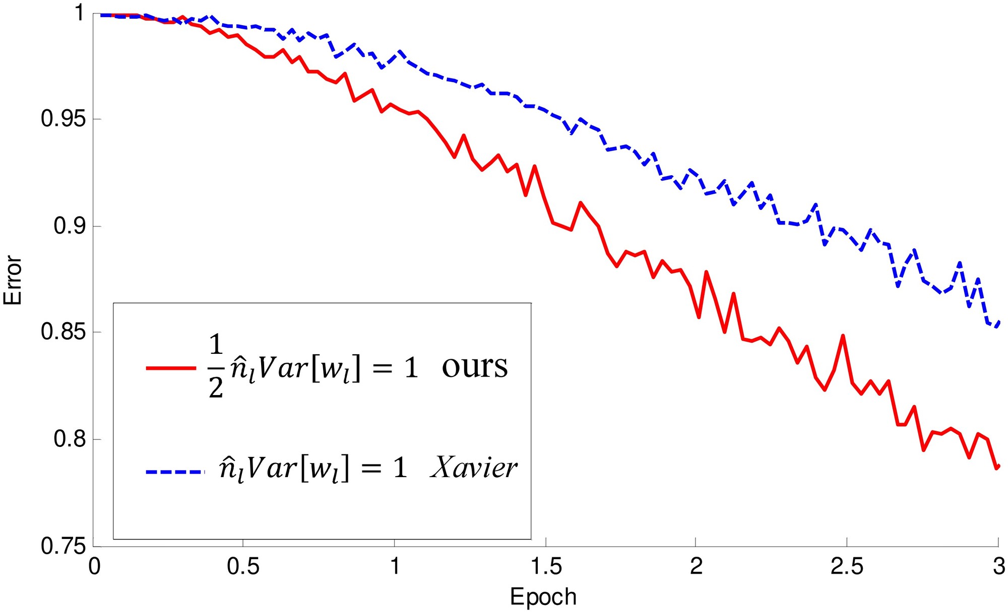
Figure 2: The convergence of a 22-layer large model (B in Table 3). The x-axis is the number of training epochs. The y-axis is the top-1 error of 3,000 random val samples, evaluated on the center crop. We use ReLU as the activation for both cases. Both our initialization (red) and “Xavier” (blue) [7] lead to convergence, but ours starts reducing error earlier.

图 2：一个 22 层 大模型（表 3 中的 B）的收敛情况。横轴是训练周期数。纵轴是 3000 个随机验证样本在中心裁剪上评估的 top-1 误差。两种情形都使用 ReLU 作为激活。我们的初始化（红色）和 “Xavier”（蓝色）[7] 都能收敛，但我们的方法更早开始降低误差。

Discussions

If the forward/backward signal is inappropriately scaled by a factor $\beta$ in each layer, then the final propagated signal will be rescaled by a factor of $\beta^{L}$ after $L$ layers, where $L$ can represent some or all layers. When $L$ is large, if $\beta>1$, this leads to extremely amplified signals and an algorithm output of infinity; if $\beta<1$, this leads to diminishing signals[^2]. In either case, the algorithm does not converge - it diverges in the former case, and stalls in the latter.

[^2]: In the presence of weight decay (l2 regularization of weights), when the gradient contributed by the logistic loss function is diminishing, the total gradient is not diminishing because of the weight decay. A way of diagnosing diminishing gradients is to check whether the gradient is modulated only by weight decay.

讨论

如果前向或反向信号在每一层被不恰当地缩放一个因子 $\beta$，那么经过 $L$ 层后，最终传播的信号会被重新缩放 $\beta^{L}$ 倍，其中 $L$ 可以表示部分或全部层。当 $L$ 很大时，若 $\beta>1$，会导致信号被极度放大，算法输出变为无穷；若 $\beta<1$，则会导致信号趋于消失。[^2] 无论哪种情形，算法都不会收敛——前者发散，后者停滞。

[^2]: 在存在权重衰减（权重的 $l_{2}$ 正则）时，当由逻辑损失贡献的梯度趋于消失时，总梯度并不会消失，因为还有权重衰减。诊断梯度是否趋于消失的一种办法，是检查梯度是否只被权重衰减调制。

Our derivation also explains why the constant standard deviation of 0.01 makes some deeper networks stall [25]. We take “model B” in the VGG team’s paper [25] as an example. This model has 10 conv layers all with 3$\times$3 filters. The filter numbers ($d_{l}$) are 64 for the 1st and 2nd layers, 128 for the 3rd and 4th layers, 256 for the 5th and 6th layers, and 512 for the rest. The std computed by Eqn.(14) ($\sqrt{2/{\hat{n}_{l}}}$) is 0.059, 0.042, 0.029, and 0.021 when the filter numbers are 64, 128, 256, and 512 respectively. If the std is initialized as 0.01, the std of the gradient propagated from conv10 to conv2 is $1/(5.9\times 4.2^{2}\times 2.9^{2}\times 2.1^{4})=1/(1.7\times 10^{4})$ of what we derive. This number may explain why diminishing gradients were observed in experiments.

我们的推导也解释了为什么恒定标准差 0.01 会使一些更深的网络停滞 [25]。我们以 VGG 团队论文 [25] 中的“模型 B”为例。该模型有 10 个卷积层，全部使用 $3\times 3$ 滤波器。滤波器数目（$d_{l}$）在第 1、2 层为 64，第 3、4 层为 128，第 5、6 层为 256，其余为 512。由式（14）算出的标准差（$\sqrt{2/{\hat{n}_{l}}}$）在滤波器数目为 64、128、256 和 512 时分别是 0.059、0.042、0.029 和 0.021。如果把标准差初始化为 0.01，那么从 conv10 传播到 conv2 的梯度标准差，将是我们推导结果的 $1/(5.9\times 4.2^{2}\times 2.9^{2}\times 2.1^{4})=1/(1.7\times 10^{4})$。这个数字或许可以解释实验中为何会观察到梯度消失。

It is also worth noticing that the variance of the input signal can be roughly preserved from the first layer to the last. In cases when the input signal is not normalized (e.g., it is in the range of $[-128,128]$), its magnitude can be so large that the softmax operator will overflow. A solution is to normalize the input signal, but this may impact other hyper-parameters. Another solution is to include a small factor on the weights among all or some layers, e.g., $\sqrt[L]{1/128}$ on $L$ layers. In practice, we use a std of 0.01 for the first two fc layers and 0.001 for the last. These numbers are smaller than they should be (e.g., $\sqrt{2/4096}$) and will address the normalization issue of images whose range is about $[-128,128]$.

还值得注意的是，输入信号的方差可以大致从第一层保持到最后一层。当输入信号未经归一化时（例如范围在 $[-128,128]$），其幅度可能大到使 softmax 算子溢出。一种办法是把输入信号归一化，但这可能影响其他超参数。另一种办法是在全部或部分层的权重上乘一个小因子，例如在 $L$ 层上乘 $\sqrt[L]{1/128}$。实践中，我们对前两个全连接层使用 0.01 的标准差，对最后一层使用 0.001。这些数字比它们应有的值更小（例如 $\sqrt{2/4096}$），将处理范围大约为 $[-128,128]$ 的图像的归一化问题。

For the initialization in the PReLU case, it is easy to show that Eqn.(10) becomes:

对 PReLU 情形的初始化，容易看出式（10）变为：

$$\frac{1}{2}(1+a^{2})n_{l}\emph{Var}[w_{l}]=1,\quad\forall l, \tag{15}$$

where $a$ is the initialized value of the coefficients. If $a=0$, it becomes the ReLU case; if $a=1$, it becomes the linear case (the same as [7]). Similarly, Eqn.(14) becomes $\frac{1}{2}(1+a^{2})\hat{n}_{l}\emph{Var}[w_{l}]=1$.

其中 $a$ 是系数的初始化值。若 $a=0$，就变成 ReLU 情形；若 $a=1$，就变成线性情形（与 [7] 相同）。类似地，式（14）变为 $\frac{1}{2}(1+a^{2})\hat{n}_{l}\emph{Var}[w_{l}]=1$。

Comparisons with “Xavier” Initialization [7]

The main difference between our derivation and the “Xavier” initialization [7] is that we address the rectifier nonlinearities[^3]. The derivation in [7] only considers the linear case, and its result is given by $n_{l}\emph{Var}[w_{l}]=1$ (the forward case), which can be implemented as a zero-mean Gaussian distribution whose std is $\sqrt{1/{n_{l}}}$. When there are $L$ layers, the std will be ${1}/{\sqrt{2}^{L}}$ of our derived std. This number, however, is not small enough to completely stall the convergence of the models actually used in our paper (Table 3, up to 22 layers) as shown by experiments. Figure 3 compares the convergence of a 22-layer model. Both methods are able to make them converge. But ours starts reducing error earlier. We also investigate the possible impact on accuracy. For the model in Table 2 (using ReLU), the “Xavier” initialization method leads to 33.90/13.44 top-1/top-5 error, and ours leads to 33.82/13.34. We have not observed clear superiority of one to the other on accuracy.

[^3]: There are other minor differences. In [7], the derived variance is adopted for uniform distributions, and the forward and backward cases are averaged. But it is straightforward to adopt their conclusion for Gaussian distributions and for the forward or backward case only.

与 “Xavier” 初始化 [7] 的比较

我们的推导与 “Xavier” 初始化 [7] 的主要差别在于，我们处理了整流非线性。[^3] [7] 中的推导只考虑线性情形，其结果由 $n_{l}\emph{Var}[w_{l}]=1$ 给出（前向情形），可以实现为均值为零、标准差为 $\sqrt{1/{n_{l}}}$ 的高斯分布。当有 $L$ 层时，该标准差将是我们推导出的标准差的 ${1}/{\sqrt{2}^{L}}$。不过，正如图中实验所示，这个数字还不足以完全阻滞本文实际使用的模型（表 3，最深 22 层）的收敛。图 3 比较了一个 22 层模型的收敛。两种方法都能使它们收敛，但我们的方法更早开始降低误差。我们也考察了可能对精度的影响。对表 2 中的模型（使用 ReLU），“Xavier” 初始化方法给出 33.90/13.44 的 top-1/top-5 误差，我们的方法给出 33.82/13.34。在精度上，我们没有观察到一方对另一方有明显优势。

[^3]: 还有一些次要差别。在 [7] 中，推导出的方差被用于均匀分布，并且对前向和反向情形取了平均。但把他们的结论改用于高斯分布、并只用于前向或只用于反向，是直截了当的。

Next, we compare the two methods on extremely deep models with up to 30 layers (27 conv and 3 fc). We add up to sixteen conv layers with 256 2$\times$2 filters in the model in Table 1. Figure 3 shows the convergence of the 30-layer model. Our initialization is able to make the extremely deep model converge. On the contrary, the “Xavier” method completely stalls the learning, and the gradients are diminishing as monitored in the experiments.

接下来，我们在最深 30 层（27 个卷积层和 3 个全连接层）的极深模型上比较这两种方法。我们在表 1 的模型中最多加入 16 个带 256 个 $2\times 2$ 滤波器的卷积层。图 3 给出了 30 层模型的收敛情况。我们的初始化能够使这一极深模型收敛。相反，“Xavier” 方法使学习完全停滞，实验中监测到梯度正在消失。

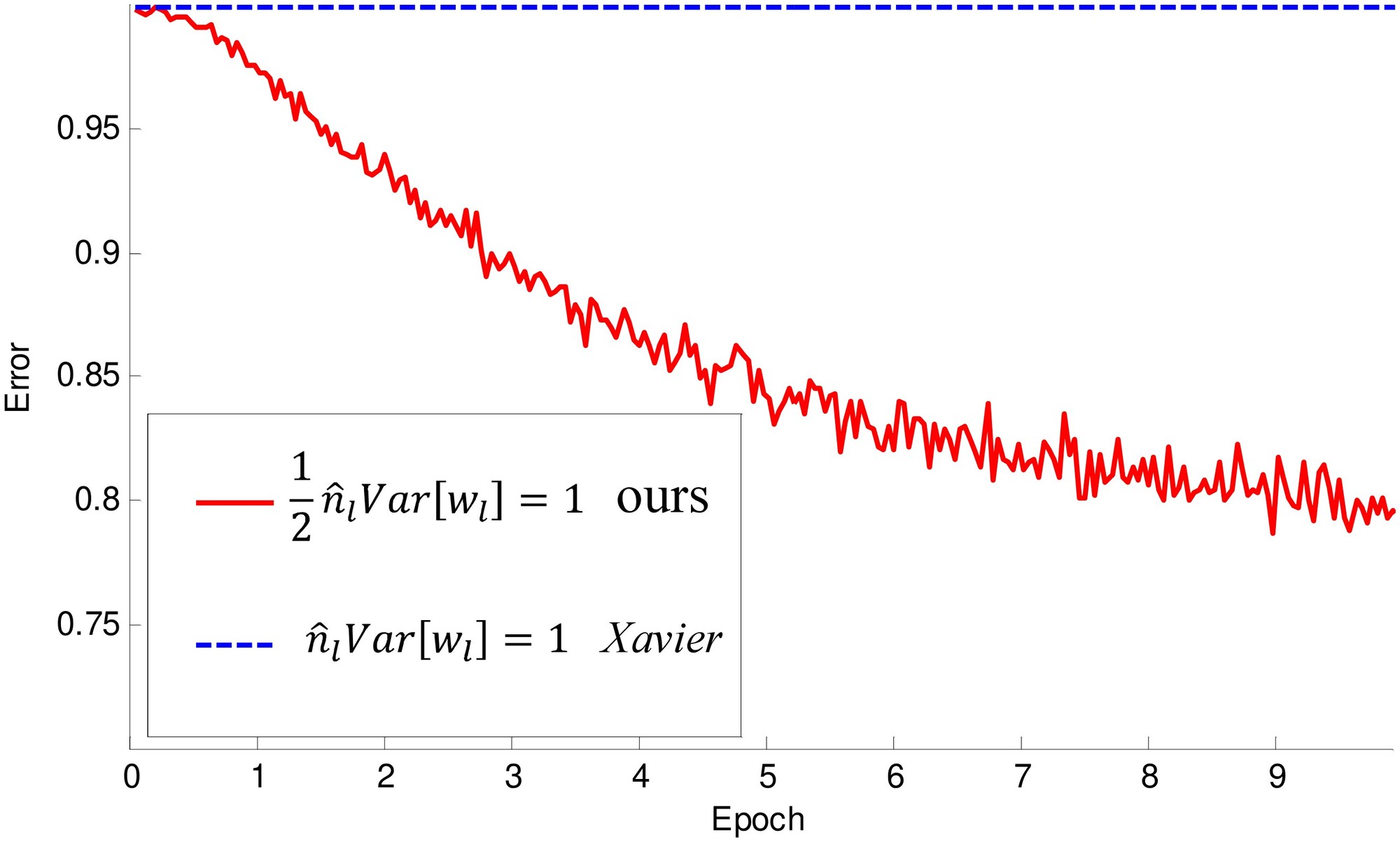
Figure 3: The convergence of a 30-layer small model (see the main text). We use ReLU as the activation for both cases. Our initialization (red) is able to make it converge. But “Xavier” (blue) [7] completely stalls - we also verify that its gradients are all diminishing. It does not converge even given more epochs.

图 3：一个 30 层小模型的收敛情况（见正文）。两种情形都使用 ReLU 作为激活。我们的初始化（红色）能够使它收敛。但 “Xavier”（蓝色）[7] 完全停滞——我们也验证了其梯度全部趋于消失。即使再增加周期，它也不会收敛。

These studies demonstrate that we are ready to investigate extremely deep, rectified models by using a more principled initialization method. But in our current experiments on ImageNet, we have not observed the benefit from training extremely deep models. For example, the aforementioned 30-layer model has 38.56/16.59 top-1/top-5 error, which is clearly worse than the error of the 14-layer model in Table 2 (33.82/13.34). Accuracy saturation or degradation was also observed in the study of small models [10], VGG’s large models [25], and in speech recognition [34]. This is perhaps because the method of increasing depth is not appropriate, or the recognition task is not enough complex.

这些研究表明，借助一种更有原则的初始化方法，我们已经可以着手研究极深的整流模型。但在我们目前的 ImageNet 实验中，尚未观察到训练极深模型带来的好处。例如，上述 30 层模型的 top-1/top-5 误差为 38.56/16.59，明显差于表 2 中 14 层模型的误差（33.82/13.34）。在对小模型 [10]、VGG 大模型 [25] 以及语音识别 [34] 的研究中，也观察到了精度饱和或下降。这也许是因为增加深度的方法并不恰当，或者识别任务还不够复杂。

Though our attempts of extremely deep models have not shown benefits, our initialization method paves a foundation for further study on increasing depth. We hope this will be helpful in other more complex tasks.

尽管我们对极深模型的尝试尚未显示出好处，我们的初始化方法为进一步研究增加深度打下了基础。我们希望这在其他更复杂的任务中会有帮助。

input size	VGG-19 [25]	model A	model B	model C
224	3$\times$3, 64	7$\times$7, 96, /2	7$\times$7, 96, /2	7$\times$7, 96, /2
3$\times$3, 64
2$\times$2 maxpool, /2
112	3$\times$3, 128
3$\times$3, 128
2$\times$2 maxpool, /2	2$\times$2 maxpool, /2	2$\times$2 maxpool, /2	2$\times$2 maxpool, /2
56	3$\times$3, 256	3$\times$3, 256	3$\times$3, 256	3$\times$3, 384
3$\times$3, 256	3$\times$3, 256	3$\times$3, 256	3$\times$3, 384
3$\times$3, 256	3$\times$3, 256	3$\times$3, 256	3$\times$3, 384
3$\times$3, 256	3$\times$3, 256	3$\times$3, 256	3$\times$3, 384
	3$\times$3, 256	3$\times$3, 256	3$\times$3, 384
		3$\times$3, 256	3$\times$3, 384
2$\times$2 maxpool, /2	2$\times$2 maxpool, /2	2$\times$2 maxpool, /2	2$\times$2 maxpool, /2
28	3$\times$3, 512	3$\times$3, 512	3$\times$3, 512	3$\times$3, 768
3$\times$3, 512	3$\times$3, 512	3$\times$3, 512	3$\times$3, 768
3$\times$3, 512	3$\times$3, 512	3$\times$3, 512	3$\times$3, 768
3$\times$3, 512	3$\times$3, 512	3$\times$3, 512	3$\times$3, 768
	3$\times$3, 512	3$\times$3, 512	3$\times$3, 768
		3$\times$3, 512	3$\times$3, 768
2$\times$2 maxpool, /2	2$\times$2 maxpool, /2	2$\times$2 maxpool, /2	2$\times$2 maxpool, /2
14	3$\times$3, 512	3$\times$3, 512	3$\times$3, 512	3$\times$3, 896
3$\times$3, 512	3$\times$3, 512	3$\times$3, 512	3$\times$3, 896
3$\times$3, 512	3$\times$3, 512	3$\times$3, 512	3$\times$3, 896
3$\times$3, 512	3$\times$3, 512	3$\times$3, 512	3$\times$3, 896
	3$\times$3, 512	3$\times$3, 512	3$\times$3, 896
		3$\times$3, 512	3$\times$3, 896
2$\times$2 maxpool, /2	spp, $\{7,3,2,1\}$	spp, $\{7,3,2,1\}$	spp, $\{7,3,2,1\}$
fc1	4096
fc2	4096
fc3	1000
depth (conv+fc)	19	19	22	22
complexity (ops., $\times 10^{10}$)	1.96	1.90	2.32	5.30

Table 3: Architectures of large models. Here “/2” denotes a stride of 2.

输入尺寸	VGG-19 [25]	模型 A	模型 B	模型 C
224	3$\times$3, 64	7$\times$7, 96, /2	7$\times$7, 96, /2	7$\times$7, 96, /2
3$\times$3, 64
2$\times$2 最大池化，/2
112	3$\times$3, 128
3$\times$3, 128
2$\times$2 最大池化，/2	2$\times$2 最大池化，/2	2$\times$2 最大池化，/2	2$\times$2 最大池化，/2
56	3$\times$3, 256	3$\times$3, 256	3$\times$3, 256	3$\times$3, 384
3$\times$3, 256	3$\times$3, 256	3$\times$3, 256	3$\times$3, 384
3$\times$3, 256	3$\times$3, 256	3$\times$3, 256	3$\times$3, 384
3$\times$3, 256	3$\times$3, 256	3$\times$3, 256	3$\times$3, 384
	3$\times$3, 256	3$\times$3, 256	3$\times$3, 384
		3$\times$3, 256	3$\times$3, 384
2$\times$2 最大池化，/2	2$\times$2 最大池化，/2	2$\times$2 最大池化，/2	2$\times$2 最大池化，/2
28	3$\times$3, 512	3$\times$3, 512	3$\times$3, 512	3$\times$3, 768
3$\times$3, 512	3$\times$3, 512	3$\times$3, 512	3$\times$3, 768
3$\times$3, 512	3$\times$3, 512	3$\times$3, 512	3$\times$3, 768
3$\times$3, 512	3$\times$3, 512	3$\times$3, 512	3$\times$3, 768
	3$\times$3, 512	3$\times$3, 512	3$\times$3, 768
		3$\times$3, 512	3$\times$3, 768
2$\times$2 最大池化，/2	2$\times$2 最大池化，/2	2$\times$2 最大池化，/2	2$\times$2 最大池化，/2
14	3$\times$3, 512	3$\times$3, 512	3$\times$3, 512	3$\times$3, 896
3$\times$3, 512	3$\times$3, 512	3$\times$3, 512	3$\times$3, 896
3$\times$3, 512	3$\times$3, 512	3$\times$3, 512	3$\times$3, 896
3$\times$3, 512	3$\times$3, 512	3$\times$3, 512	3$\times$3, 896
	3$\times$3, 512	3$\times$3, 512	3$\times$3, 896
		3$\times$3, 512	3$\times$3, 896
2$\times$2 最大池化，/2	spp, $\{7,3,2,1\}$	spp, $\{7,3,2,1\}$	spp, $\{7,3,2,1\}$
fc1	4096
fc2	4096
fc3	1000
深度（conv+fc）	19	19	22	22
复杂度（运算次数，$\times 10^{10}$）	1.96	1.90	2.32	5.30

表 3：大模型的结构。这里“/2”表示步长为 2。

2.3 Architectures

2.3 网络结构

The above investigations provide guidelines of designing our architectures, introduced as follows.

上述研究为我们的结构设计提供了指南，介绍如下。

Our baseline is the 19-layer model (A) in Table 3. For a better comparison, we also list the VGG-19 model [25]. Our model A has the following modifications on VGG-19: (i) in the first layer, we use a filter size of 7$\times$7 and a stride of 2; (ii) we move the other three conv layers on the two largest feature maps (224, 112) to the smaller feature maps (56, 28, 14). The time complexity (Table 3, last row) is roughly unchanged because the deeper layers have more filters; (iii) we use spatial pyramid pooling (SPP) [11] before the first fc layer. The pyramid has 4 levels - the numbers of bins are 7$\times$7, 3$\times$3, 2$\times$2, and 1$\times$1, for a total of 63 bins.

我们的基线是表 3 中的 19 层模型（A）。为便于比较，我们也列出了 VGG-19 模型 [25]。我们的模型 A 相对 VGG-19 有如下改动：（i）在第一层，我们使用 $7\times 7$ 的滤波器和步长 2；（ii）我们把另外三个位于最大两张特征图（224、112）上的卷积层，移到更小的特征图（56、28、14）上。时间复杂度（表 3，最后一行）大致不变，因为更深的层有更多滤波器；（iii）我们在第一个全连接层之前使用空间金字塔池化（SPP）[11]。金字塔有 4 个层级——箱子数目为 $7\times 7$、$3\times 3$、$2\times 2$ 和 $1\times 1$，共 63 个箱子。

It is worth noticing that we have no evidence that our model A is a better architecture than VGG-19, though our model A has better results than VGG-19’s result reported by [25]. In our earlier experiments with less scale augmentation, we observed that our model A and our reproduced VGG-19 (with SPP and our initialization) are comparable. The main purpose of using model A is for faster running speed. The actual running time of the conv layers on larger feature maps is slower than those on smaller feature maps, when their time complexity is the same. In our four-GPU implementation, our model A takes 2.6s per mini-batch (128), and our reproduced VGG-19 takes 3.0s, evaluated on four Nvidia K20 GPUs.

值得注意的是，我们并没有证据表明模型 A 在结构上优于 VGG-19，尽管我们的模型 A 比 [25] 报告的 VGG-19 结果更好。在我们较早、尺度增强较弱的实验中，观察到模型 A 与我们复现的 VGG-19（加上 SPP 和我们的初始化）表现相当。使用模型 A 的主要目的是为了跑得更快。当时间复杂度相同时，较大特征图上卷积层的实际运行时间比小特征图上更慢。在我们的四 GPU 实现中，模型 A 每个小批量（128）耗时 2.6 秒，我们复现的 VGG-19 耗时 3.0 秒，评测平台是四块 Nvidia K20 GPU。

In Table 3, our model B is a deeper version of A. It has three extra conv layers. Our model C is a wider (with more filters) version of B. The width substantially increases the complexity, and its time complexity is about 2.3$\times$ of B (Table 3, last row). Training A/B on four K20 GPUs, or training C on eight K40 GPUs, takes about 3-4 weeks.

在表 3 中，我们的模型 B 是 A 的更深版本，多了三个卷积层。我们的模型 C 是 B 的更宽版本（滤波器更多）。宽度显著增加了复杂度，其时间复杂度约为 B 的 2.3 倍（表 3，最后一行）。在四块 K20 GPU 上训练 A/B，或在八块 K40 GPU 上训练 C，大约需要 3 到 4 周。

We choose to increase the model width instead of depth, because deeper models have only diminishing improvement or even degradation on accuracy. In recent experiments on small models [10], it has been found that aggressively increasing the depth leads to saturated or degraded accuracy. In the VGG paper [25], the 16-layer and 19-layer models perform comparably. In the speech recognition research of [34], the deep models degrade when using more than 8 hidden layers (all being fc). We conjecture that similar degradation may also happen on larger models for ImageNet. We have monitored the training procedures of some extremely deep models (with 3 to 9 layers added on B in Table 3), and found both training and testing error rates degraded in the first 20 epochs (but we did not run to the end due to limited time budget, so there is not yet solid evidence that these large and overly deep models will ultimately degrade). Because of the possible degradation, we choose not to further increase the depth of these large models.

我们选择增加模型宽度而不是深度，因为更深的模型在精度上只有越来越小的改进，甚至会下降。在近期对小模型的实验中 [10]，人们发现过激地增加深度会导致精度饱和或下降。在 VGG 的论文 [25] 中，16 层和 19 层模型表现相当。在 [34] 的语音识别研究中，当隐层超过 8 层（全部是全连接层）时，深层模型会变差。我们推测，类似的下降也可能出现在更大的 ImageNet 模型上。我们监测过一些极深模型的训练过程（在表 3 的模型 B 上再加 3 到 9 层），发现前 20 个周期中训练误差和测试误差都变差了（但受时间预算所限我们没有跑完，因此还没有充分证据表明这些又大又过深的模型最终一定会变差）。由于可能出现下降，我们选择不再进一步增加这些大模型的深度。

On the other hand, the recent research [5] on small datasets suggests that the accuracy should improve from the increased number of parameters in conv layers. This number depends on the depth and width. So we choose to increase the width of the conv layers to obtain a higher-capacity model.

另一方面，近期在小数据集上的研究 [5] 表明，精度应当随着卷积层参数数目的增加而提升。这一数目取决于深度和宽度。因此我们选择增加卷积层的宽度，以得到容量更高的模型。

While all models in Table 3 are very large, we have not observed severe overfitting. We attribute this to the aggressive data augmentation used throughout the whole training procedure, as introduced below.

尽管表 3 中的模型都非常大，我们并没有观察到严重的过拟合。我们把这一点归因于整个训练过程中使用的较强数据增强，介绍如下。

3 Implementation Details

3 实现细节

Training

Our training algorithm mostly follows [16, 13, 2, 11, 25]. From a resized image whose shorter side is $s$, a 224$\times$224 crop is randomly sampled, with the per-pixel mean subtracted. The scale $s$ is randomly jittered in the range of $[256,512]$, following [25]. One half of the random samples are flipped horizontally [16]. Random color altering [16] is also used.

训练

我们的训练算法大多沿用 [16, 13, 2, 11, 25]。从较短边为 $s$ 的缩放图像中，随机采样一个 $224\times 224$ 的裁剪，并减去逐像素均值。尺度 $s$ 在 $[256,512]$ 范围内随机抖动，做法遵循 [25]。一半的随机样本做水平翻转 [16]。也使用了随机颜色扰动 [16]。

Unlike [25] that applies scale jittering only during fine-tuning, we apply it from the beginning of training. Further, unlike [25] that initializes a deeper model using a shallower one, we directly train the very deep model using our initialization described in Sec. 2.2 (we use Eqn.(14)). Our end-to-end training may help improve accuracy, because it may avoid poorer local optima.

与 [25] 只在微调时使用尺度抖动不同，我们从训练一开始就使用它。此外，与 [25] 用较浅模型初始化较深模型不同，我们用第 2.2 节所述的初始化（我们使用式（14））直接训练很深的模型。这种端到端训练可能有助于提升精度，因为它或许能避开更差的局部最优。

Other hyper-parameters that might be important are as follows. The weight decay is 0.0005, and momentum is 0.9. Dropout (50%) is used in the first two fc layers. The mini-batch size is fixed as 128. The learning rate is 1e-2, 1e-3, and 1e-4, and is switched when the error plateaus. The total number of epochs is about 80 for each model.

其他可能重要的超参数如下。权重衰减为 0.0005，动量为 0.9。前两个全连接层使用 dropout（50%）。小批量大小固定为 128。学习率为 1e-2、1e-3 和 1e-4，在误差进入平台期时切换。每个模型大约训练 80 个周期。

Testing

We adopt the strategy of “multi-view testing on feature maps” used in the SPP-net paper [11]. We further improve this strategy using the dense sliding window method in [24, 25].

测试

我们采用 SPP-net 论文 [11] 中使用的“在特征图上做多视图测试”策略，并用 [24, 25] 中的密集滑动窗口方法进一步改进。

We first apply the convolutional layers on the resized full image and obtain the last convolutional feature map. In the feature map, each 14$\times$14 window is pooled using the SPP layer [11]. The fc layers are then applied on the pooled features to compute the scores. This is also done on the horizontally flipped images. The scores of all dense sliding windows are averaged [24, 25]. We further combine the results at multiple scales as in [11].

我们首先在缩放后的整幅图像上应用卷积层，得到最后一张卷积特征图。在特征图中，每个 $14\times 14$ 窗口用 SPP 层 [11] 做池化。然后把全连接层作用在池化后的特征上以计算分数。这一过程也在水平翻转的图像上进行。所有密集滑动窗口的分数取平均 [24, 25]。我们还按 [11] 的做法结合多个尺度的结果。

Multi-GPU Implementation

We adopt a simple variant of Krizhevsky’s method [15] for parallel training on multiple GPUs. We adopt “data parallelism” [15] on the conv layers. The GPUs are synchronized before the first fc layer. Then the forward/backward propagations of the fc layers are performed on a single GPU - this means that we do not parallelize the computation of the fc layers. The time cost of the fc layers is low, so it is not necessary to parallelize them. This leads to a simpler implementation than the “model parallelism” in [15]. Besides, model parallelism introduces some overhead due to the communication of filter responses, and is not faster than computing the fc layers on just a single GPU.

多 GPU 实现

我们采用 Krizhevsky 方法 [15] 的一个简单变体，在多块 GPU 上并行训练。我们在卷积层上采用“数据并行” [15]。各 GPU 在第一个全连接层之前同步。然后全连接层的前向和反向传播在单块 GPU 上完成——这意味着我们并不并行化全连接层的计算。全连接层的时间开销较低，因此没有必要并行化它们。这带来了比 [15] 中“模型并行”更简单的实现。此外，模型并行会因滤波器响应的通信而引入一些开销，并不比只在单块 GPU 上计算全连接层更快。

We implement the above algorithm on our modification of the Caffe library [14]. We do not increase the mini-batch size (128) because the accuracy may be decreased [15]. For the large models in this paper, we have observed a 3.8x speedup using 4 GPUs, and a 6.0x speedup using 8 GPUs.

我们在修改过的 Caffe 库 [14] 上实现了上述算法。我们不增加小批量大小（128），因为精度可能会下降 [15]。对本文中的大模型，我们观察到使用 4 块 GPU 有 3.8 倍加速，使用 8 块 GPU 有 6.0 倍加速。

4 Experiments on ImageNet

4 在 ImageNet 上的实验

We perform the experiments on the 1000-class ImageNet 2012 dataset [22] which contains about 1.2 million training images, 50,000 validation images, and 100,000 test images (with no published labels). The results are measured by top-1/top-5 error rates [22]. We only use the provided data for training. All results are evaluated on the validation set, except for the final results in Table 7, which are evaluated on the test set. The top-5 error rate is the metric officially used to rank the methods in the classification challenge [22].

我们在 1000 类 ImageNet 2012 数据集 [22] 上做实验，其中约有 120 万张训练图像、5 万张验证图像和 10 万张测试图像（没有公开标签）。结果用 top-1/top-5 误差率衡量 [22]。我们只使用提供的数据来训练。除表 7 中的最终结果在测试集上评估外，全部结果都在验证集上评估。top-5 误差率是该分类挑战中正式用来给方法排序的指标 [22]。

model A	ReLU	PReLU
scale $s$	top-1	top-5	top-1	top-5
256	26.25	8.25	25.81	8.08
384	24.77	7.26	24.20	7.03
480	25.46	7.63	24.83	7.39
multi-scale	24.02	6.51	22.97	6.28

Table 4: Comparisons between ReLU/PReLU on model A in ImageNet 2012 using dense testing.

模型 A	ReLU	PReLU
尺度 $s$	top-1	top-5	top-1	top-5
256	26.25	8.25	25.81	8.08
384	24.77	7.26	24.20	7.03
480	25.46	7.63	24.83	7.39
多尺度	24.02	6.51	22.97	6.28

表 4：在 ImageNet 2012 上用密集测试比较模型 A 的 ReLU 与 PReLU。

Comparisons between ReLU and PReLU

In Table 4, we compare ReLU and PReLU on the large model A. We use the channel-wise version of PReLU. For fair comparisons, both ReLU/PReLU models are trained using the same total number of epochs, and the learning rates are also switched after running the same number of epochs.

ReLU 与 PReLU 的比较

在表 4 中，我们在大模型 A 上比较 ReLU 和 PReLU。我们使用逐通道版本的 PReLU。为公平比较，ReLU 与 PReLU 模型都用相同的总周期数训练，学习率也在运行相同周期数后切换。

Table 4 shows the results at three scales and the multi-scale combination. The best single scale is 384, possibly because it is in the middle of the jittering range $[256,512]$. For the multi-scale combination, PReLU reduces the top-1 error by 1.05% and the top-5 error by 0.23% compared with ReLU. The results in Table 2 and Table 4 consistently show that PReLU improves both small and large models. This improvement is obtained with almost no computational cost.

表 4 给出了三个尺度以及多尺度组合的结果。最好的单尺度是 384，可能是因为它位于抖动范围 $[256,512]$ 的中间。对多尺度组合，与 ReLU 相比，PReLU 把 top-1 误差降低 1.05 个百分点，把 top-5 误差降低 0.23 个百分点。表 2 和表 4 的结果一贯表明，PReLU 对小模型和大模型都有改进。这一改进几乎不增加计算代价。

Comparisons of Single-model Results

Next we compare single-model results. We first show 10-view testing results [16] in Table 7. Here, each view is a 224-crop. The 10-view results of VGG-16 are based on our testing using the publicly released model [25] as it is not reported in [25]. Our best 10-view result is 7.38% (Table 7). Our other models also outperform the existing results.

单模型结果的比较

接下来我们比较单模型结果。我们首先在表 7 中给出 10 视图测试结果 [16]。这里，每个视图是一个 224 的裁剪。VGG-16 的 10 视图结果基于我们使用公开发布模型 [25] 所做的测试，因为 [25] 中没有报告。我们最好的 10 视图结果是 7.38%（表 7）。我们的其他模型也超过了已有结果。

Table 7 shows the comparisons of single-model results, which are all obtained using multi-scale and multi-view (or dense) test. Our results are denoted as MSRA. Our baseline model (A+ReLU, 6.51%) is already substantially better than the best existing single-model result of 7.1% reported for VGG-19 in the latest update of [25] (arXiv v5). We believe that this gain is mainly due to our end-to-end training, without the need of pre-training shallow models.

表 7 给出了单模型结果的比较，这些结果都是用多尺度和多视图（或密集）测试得到的。我们的结果记为 MSRA。我们的基线模型（A+ReLU，6.51%）已经明显高于 [25] 最新更新（arXiv v5）中为 VGG-19 报告的最好已有单模型结果 7.1%。我们认为，这一收益主要来自端到端训练，而不需要先预训练较浅的模型。

Moreover, our best single model (C, PReLU) has 5.71% top-5 error. This result is even better than all previous multi-model results (Table 7). Comparing A+PReLU with B+PReLU, we see that the 19-layer model and the 22-layer model perform comparably. On the other hand, increasing the width (C vs. B, Table 7) can still improve accuracy. This indicates that when the models are deep enough, the width becomes an essential factor for accuracy.

此外，我们最好的单模型（C，PReLU）有 5.71% 的 top-5 误差。这一结果甚至好于此前所有的多模型结果（表 7）。比较 A+PReLU 与 B+PReLU，可以看到 19 层模型与 22 层模型表现相当。另一方面，增加宽度（表 7 中 C 对 B）仍能提升精度。这表明，当模型已经足够深时，宽度成为影响精度的关键因素。

model	top-1	top-5
MSRA [11]	29.68	10.95
VGG-16 [25]	28.07*†*	9.33*†*
GoogLeNet [29]	-	9.15
A, ReLU	26.48	8.59
A, PReLU	25.59	8.23
B, PReLU	25.53	8.13
C, PReLU	24.27	7.38

	team	top-1	top-5
in competition    ILSVRC 14	MSRA [11]	27.86	9.08*†*
VGG [25]	-	8.43*†*
GoogLeNet [29]	-	7.89
post-competition	VGG [25] (arXiv v2)	24.8	7.5
VGG [25] (arXiv v5)	24.4	7.1
Baidu [32]	24.88	7.42
MSRA (A, ReLU)	24.02	6.51
MSRA (A, PReLU)	22.97	6.28
MSRA (B, PReLU)	22.85	6.27
MSRA (C, PReLU)	21.59	5.71

	team	top-5 (test)
in competition    ILSVRC 14	MSRA, SPP-nets [11]	8.06
VGG [25]	7.32
GoogLeNet [29]	6.66
post-competition	VGG [25] (arXiv v5)	6.8
Baidu [32]	5.98
MSRA, PReLU-nets	4.94

Table 5: The single-model 10-view results for ImageNet 2012 val set. †: Based on our tests.

Table 6: The single-model results for ImageNet 2012 val set. †: Evaluated from the test set.

Table 7: The multi-model results for the ImageNet 2012 test set.

模型	top-1	top-5
MSRA [11]	29.68	10.95
VGG-16 [25]	28.07*†*	9.33*†*
GoogLeNet [29]	-	9.15
A, ReLU	26.48	8.59
A, PReLU	25.59	8.23
B, PReLU	25.53	8.13
C, PReLU	24.27	7.38

	团队	top-1	top-5
竞赛中  ILSVRC 14	MSRA [11]	27.86	9.08*†*
VGG [25]	-	8.43*†*
GoogLeNet [29]	-	7.89
竞赛后	VGG [25]（arXiv v2）	24.8	7.5
VGG [25]（arXiv v5）	24.4	7.1
Baidu [32]	24.88	7.42
MSRA（A, ReLU）	24.02	6.51
MSRA（A, PReLU）	22.97	6.28
MSRA（B, PReLU）	22.85	6.27
MSRA（C, PReLU）	21.59	5.71

	团队	top-5（测试集）
竞赛中  ILSVRC 14	MSRA, SPP-nets [11]	8.06
VGG [25]	7.32
GoogLeNet [29]	6.66
竞赛后	VGG [25]（arXiv v5）	6.8
Baidu [32]	5.98
MSRA, PReLU-nets	4.94

表 5：ImageNet 2012 验证集上的单模型 10 视图 结果。†：基于我们的测试。

表 6：ImageNet 2012 验证集上的单模型结果。†：由测试集评估。

表 7：ImageNet 2012 测试集上的多模型结果。

Comparisons of Multi-model Results

We combine six models including those in Table 7. For the time being we have trained only one model with architecture C. The other models have accuracy inferior to C by considerable margins. We conjecture that we can obtain better results by using fewer stronger models.

多模型结果的比较

我们把包括表 7 中那些在内的六个模型组合起来。目前我们只训练了一个结构为 C 的模型。其他模型的精度比 C 差出相当的间隔。我们推测，用更少但更强的模型可以得到更好的结果。

The multi-model results are in Table 7. Our result is 4.94% top-5 error on the test set. This number is evaluated by the ILSVRC server, because the labels of the test set are not published. Our result is 1.7% better than the ILSVRC 2014 winner (GoogLeNet, 6.66% [29]), which represents a $\sim$26% relative improvement. This is also a $\sim$17% relative improvement over the latest result (Baidu, 5.98% [32]).

多模型结果见表 7。我们的结果是测试集上 4.94% 的 top-5 误差。这一数字由 ILSVRC 服务器评估，因为测试集的标签并未公开。我们的结果比 ILSVRC 2014 获胜者（GoogLeNet，6.66% [29]）好 1.7 个百分点，相当于约 26% 的相对提升。这也相对最新结果（Baidu，5.98% [32]）有约 17% 的相对提升。

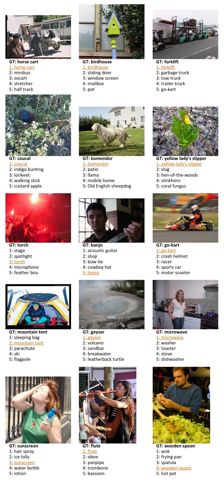
Figure 4: Example validation images successfully classified by our method. For each image, the ground-truth label and the top-5 labels predicted by our method are listed.

图 4：我们的方法成功分类的验证图像示例。对每张图像，列出了真实标签以及我们的方法预测的 top-5 标签。

Analysis of Results

Figure 4 shows some example validation images successfully classified by our method. Besides the correctly predicted labels, we also pay attention to the other four predictions in the top-5 results. Some of these four labels are other objects in the multi-object images, e.g., the “horse-cart” image (Figure 4, row 1, col 1) contains a “mini-bus” and it is also recognized by the algorithm. Some of these four labels are due to the uncertainty among similar classes, e.g., the “coucal” image (Figure 4, row 2, col 1) has predicted labels of other bird species.

结果分析

图 4 给出了一些被我们的方法成功分类的验证图像示例。除了正确预测的标签，我们也关注 top-5 结果中的另外四个预测。其中有些是多物体图像中的其他物体，例如 “horse-cart” 图像（图 4，第 1 行第 1 列）中包含一辆 “mini-bus”，算法也识别了出来。另一些则来自相似类别之间的不确定性，例如 “coucal” 图像（图 4，第 2 行第 1 列）的预测标签是其他鸟类。

Figure 7 shows the per-class top-5 error of our result (average of 4.94%) on the test set, displayed in ascending order. Our result has zero top-5 error in 113 classes - the images in these classes are all correctly classified. The three classes with the highest top-5 error are “letter opener” (49%), “spotlight” (38%), and “restaurant” (36%). The error is due to the existence of multiple objects, small objects, or large intra-class variance. Figure 5 shows some example images misclassified by our method in these three classes. Some of the predicted labels still make some sense.

图 7 给出了我们的结果在测试集上按类统计的 top-5 误差（平均为 4.94%），按升序显示。我们的结果在 113 个类别上 top-5 误差为零——这些类别中的图像全部被正确分类。top-5 误差最高的三个类别是 “letter opener”（49%）、“spotlight”（38%）和 “restaurant”（36%）。误差来自多个物体、小物体或较大的类内方差。图 5 给出了我们的方法在这三个类别中分错的一些示例图像。其中一些预测标签仍然说得通。

In Figure 7, we show the per-class difference of top-5 error rates between our result (average of 4.94%) and our team’s in-competition result in ILSVRC 2014 (average of 8.06%). The error rates are reduced in 824 classes, unchanged in 127 classes, and increased in 49 classes.

在图 7 中，我们给出了我们的结果（平均 4.94%）与我们团队在 ILSVRC 2014 竞赛中的结果（平均 8.06%）按类统计的 top-5 误差率之差。误差率在 824 个类别上降低，在 127 个类别上不变，在 49 个类别上升高。

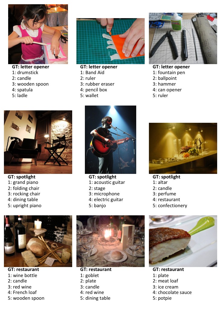
Figure 5: Example validation images incorrectly classified by our method, in the three classes with the highest top-5 test error. Top: “letter opener” (49% top-5 test error). Middle: “spotlight” (38%). Bottom: “restaurant” (36%). For each image, the ground-truth label and the top-5 labels predicted by our method are listed.

图 5：我们的方法错误分类的验证图像示例，取自 top-5 测试误差最高的三个类别。上：“letter opener”（49% 的 top-5 测试误差）。中：“spotlight”（38%）。下：“restaurant”（36%）。对每张图像，列出了真实标签以及我们的方法预测的 top-5 标签。

Comparisons with Human Performance from [22]

Russakovsky et al. [22] recently reported that human performance yields a 5.1% top-5 error on the ImageNet dataset. This number is achieved by a human annotator who is well trained on the validation images to be better aware of the existence of relevant classes. When annotating the test images, the human annotator is given a special interface, where each class title is accompanied by a row of 13 example training images. The reported human performance is estimated on a random subset of 1500 test images.

与 [22] 中人类表现的比较

Russakovsky 等人 [22] 最近报告，人类表现在 ImageNet 数据集上给出 5.1% 的 top-5 误差。这一数字由一名在验证图像上经过充分训练的标注者达到，以便更好地了解相关类别的存在。在标注测试图像时，该标注者使用一个特殊界面，每个类名旁边附有一行 13 张示例训练图像。报告的人类表现是在 1500 张随机测试图像子集上估计的。

Our result (4.94%) exceeds the reported human-level performance. To our knowledge, our result is the first published instance of surpassing humans on this visual recognition challenge. The analysis in [22] reveals that the two major types of human errors come from fine-grained recognition and class unawareness. The investigation in [22] suggests that algorithms can do a better job on fine-grained recognition (e.g., 120 species of dogs in the dataset). The second row of Figure 4 shows some example fine-grained objects successfully recognized by our method - “coucal”, “komondor”, and “yellow lady’s slipper”. While humans can easily recognize these objects as a bird, a dog, and a flower, it is nontrivial for most humans to tell their species. On the negative side, our algorithm still makes mistakes in cases that are not difficult for humans, especially for those requiring context understanding or high-level knowledge (e.g., the “spotlight” images in Figure 5).

我们的结果（4.94%）超过了所报告的人类水平表现。据我们所知，这是在该视觉识别挑战上超过人类的首个公开发表实例。[22] 中的分析表明，人类误差的两类主要来源是细粒度识别和对类别不够熟悉。[22] 中的考察表明，算法可以在细粒度识别上做得更好（例如数据集中的 120 种狗）。图 4 的第二行给出了一些被我们的方法成功识别的细粒度物体示例——“coucal”、“komondor” 和 “yellow lady’s slipper”。人类可以轻松把这些物体认作鸟、狗和花，但对大多数人来说，要说出它们的具体物种并不容易。另一方面，我们的算法仍会在对人类并不困难的情形下出错，尤其是那些需要上下文理解或高层知识的情形（例如图 5 中的 “spotlight” 图像）。

While our algorithm produces a superior result on this particular dataset, this does not indicate that machine vision outperforms human vision on object recognition in general. On recognizing elementary object categories (i.e., common objects or concepts in daily lives) such as the Pascal VOC task [6], machines still have obvious errors in cases that are trivial for humans. Nevertheless, we believe that our results show the tremendous potential of machine algorithms to match human-level performance on visual recognition.

尽管我们的算法在这一特定数据集上给出了更好的结果，这并不表明机器视觉在一般的物体识别上已经超过人类视觉。在识别基本物体类别（即日常生活中的常见物体或概念）时，例如 Pascal VOC 任务 [6]，机器仍然会在对人类来说很平常的情形中出现明显错误。尽管如此，我们相信这些结果显示了机器算法在视觉识别上达到人类水平表现的巨大潜力。

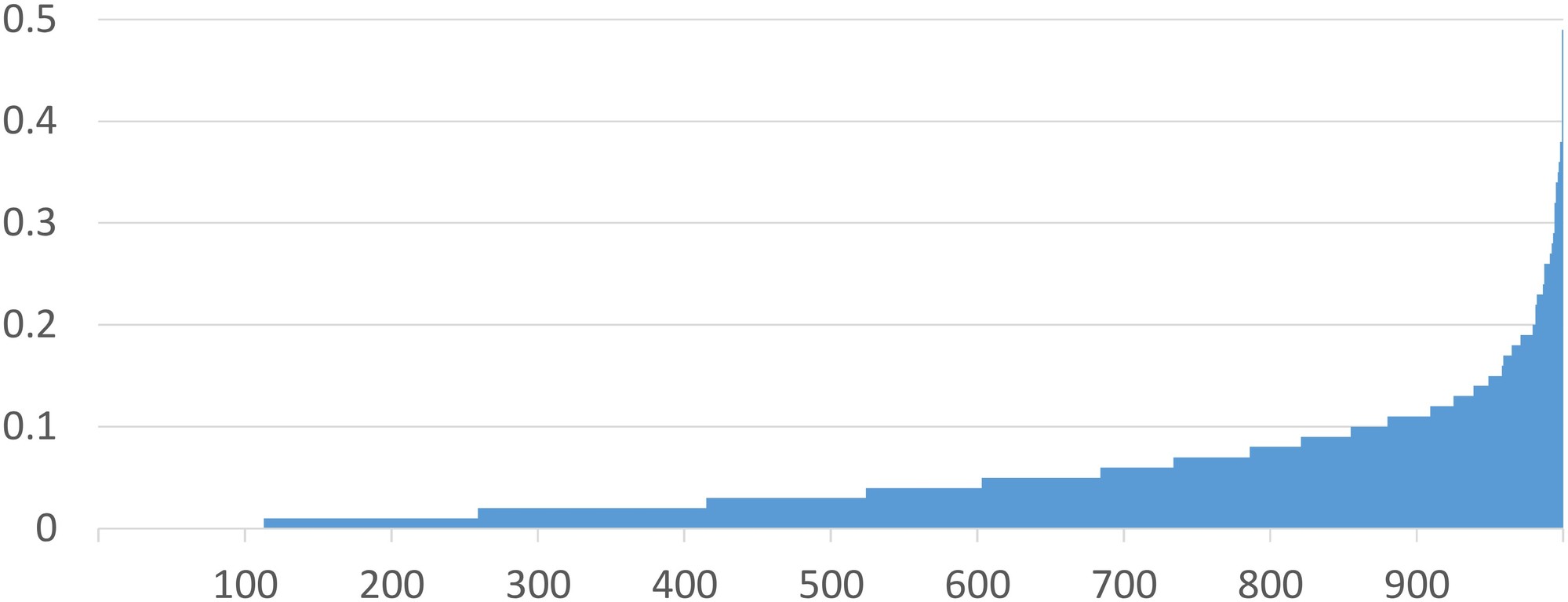
Figure 6: The per-class top-5 errors of our result (average of 4.94%) on the test set. Errors are displayed in ascending order.

图 6：我们的结果在测试集上按类统计的 top-5 误差（平均为 4.94%）。误差按升序显示。

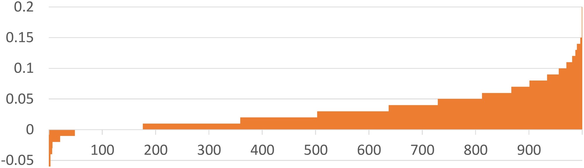
Figure 7: The difference of top-5 error rates between our result (average of 4.94%) and our team’s in-competition result for ILSVRC 2014 (average of 8.06%) on the test set, displayed in ascending order. A positive number indicates a reduced error rate.

图 7：我们的结果（平均 4.94%）与我们团队在 ILSVRC 2014 竞赛中的结果（平均 8.06%）在测试集上按类统计的 top-5 误差率之差，按升序显示。正数表示误差率降低。

References

参考文献

[1] F. Agostinelli, M. Hoffman, P. Sadowski, and P. Baldi. Learning activation functions to improve deep neural networks. arXiv:1412.6830 , 2014.

[2] K. Chatfield, K. Simonyan, A. Vedaldi, and A. Zisserman. Return of the devil in the details: Delving deep into convolutional nets. In BMVC , 2014.

[3] D. Ciresan, U. Meier, and J. Schmidhuber. Multi-column deep neural networks for image classification. In CVPR , 2012.

[4] J. Deng, W. Dong, R. Socher, L.-J. Li, K. Li, and L. Fei-Fei. Imagenet: A large-scale hierarchical image database. In CVPR , 2009.

[5] D. Eigen, J. Rolfe, R. Fergus, and Y. LeCun. Understanding deep architectures using a recursive convolutional network. arXiv:1312.1847 , 2013.

[6] M. Everingham, L. Van Gool, C. K. Williams, J. Winn, and A. Zisserman. The Pascal Visual Object Classes (VOC) Challenge. IJCV , pages 303–338, 2010.

[7] X. Glorot and Y. Bengio. Understanding the difficulty of training deep feedforward neural networks. In International Conference on Artificial Intelligence and Statistics , pages 249–256, 2010.

[8] X. Glorot, A. Bordes, and Y. Bengio. Deep sparse rectifier networks. In Proceedings of the 14th International Conference on Artificial Intelligence and Statistics , pages 315–323, 2011.

[9] I. J. Goodfellow, D. Warde-Farley, M. Mirza, A. Courville, and Y. Bengio. Maxout networks. arXiv:1302.4389 , 2013.

[10] K. He and J. Sun. Convolutional neural networks at constrained time cost. arXiv:1412.1710 , 2014.

[11] K. He, X. Zhang, S. Ren, and J. Sun. Spatial pyramid pooling in deep convolutional networks for visual recognition. arXiv:1406.4729v2 , 2014.

[12] G. E. Hinton, N. Srivastava, A. Krizhevsky, I. Sutskever, and R. R. Salakhutdinov. Improving neural networks by preventing co-adaptation of feature detectors. arXiv:1207.0580 , 2012.

[13] A. G. Howard. Some improvements on deep convolutional neural network based image classification. arXiv:1312.5402 , 2013.

[14] Y. Jia, E. Shelhamer, J. Donahue, S. Karayev, J. Long, R. Girshick, S. Guadarrama, and T. Darrell. Caffe: Convolutional architecture for fast feature embedding. arXiv:1408.5093 , 2014.

[15] A. Krizhevsky. One weird trick for parallelizing convolutional neural networks. arXiv:1404.5997 , 2014.

[16] A. Krizhevsky, I. Sutskever, and G. Hinton. Imagenet classification with deep convolutional neural networks. In NIPS , 2012.

[17] Y. LeCun, B. Boser, J. S. Denker, D. Henderson, R. E. Howard, W. Hubbard, and L. D. Jackel. Backpropagation applied to handwritten zip code recognition. Neural computation , 1989.

[18] C.-Y. Lee, S. Xie, P. Gallagher, Z. Zhang, and Z. Tu. Deeply-supervised nets. arXiv:1409.5185 , 2014.

[19] M. Lin, Q. Chen, and S. Yan. Network in network. arXiv:1312.4400 , 2013.

[20] A. L. Maas, A. Y. Hannun, and A. Y. Ng. Rectifier nonlinearities improve neural network acoustic models. In ICML , 2013.

[21] V. Nair and G. E. Hinton. Rectified linear units improve restricted boltzmann machines. In ICML , pages 807–814, 2010.

[22] O. Russakovsky, J. Deng, H. Su, J. Krause, S. Satheesh, S. Ma, Z. Huang, A. Karpathy, A. Khosla, M. Bernstein, et al. Imagenet large scale visual recognition challenge. arXiv:1409.0575 , 2014.

[23] A. M. Saxe, J. L. McClelland, and S. Ganguli. Exact solutions to the nonlinear dynamics of learning in deep linear neural networks. arXiv:1312.6120 , 2013.

[24] P. Sermanet, D. Eigen, X. Zhang, M. Mathieu, R. Fergus, and Y. LeCun. Overfeat: Integrated recognition, localization and detection using convolutional networks. 2014.

[25] K. Simonyan and A. Zisserman. Very deep convolutional networks for large-scale image recognition. arXiv:1409.1556 , 2014.

[26] N. Srivastava, G. Hinton, A. Krizhevsky, I. Sutskever, and R. Salakhutdinov. Dropout: A simple way to prevent neural networks from overfitting. The Journal of Machine Learning Research , pages 1929–1958, 2014.

[27] R. K. Srivastava, J. Masci, S. Kazerounian, F. Gomez, and J. Schmidhuber. Compete to compute. In NIPS , pages 2310–2318, 2013.

[28] Y. Sun, Y. Chen, X. Wang, and X. Tang. Deep learning face representation by joint identification-verification. In NIPS , 2014.

[29] C. Szegedy, W. Liu, Y. Jia, P. Sermanet, S. Reed, D. Anguelov, D. Erhan, V. Vanhoucke, and A. Rabinovich. Going deeper with convolutions. arXiv:1409.4842 , 2014.

[30] Y. Taigman, M. Yang, M. Ranzato, and L. Wolf. Deepface: Closing the gap to human-level performance in face verification. In CVPR , 2014.

[31] L. Wan, M. Zeiler, S. Zhang, Y. L. Cun, and R. Fergus. Regularization of neural networks using dropconnect. In ICML , pages 1058–1066, 2013.

[32] R. Wu, S. Yan, Y. Shan, Q. Dang, and G. Sun. Deep image: Scaling up image recognition. arXiv:1501.02876 , 2015.

[33] M. D. Zeiler and R. Fergus. Visualizing and understanding convolutional neural networks. In ECCV , 2014.

[34] M. D. Zeiler, M. Ranzato, R. Monga, M. Mao, K. Yang, Q. V. Le, P. Nguyen, A. Senior, V. Vanhoucke, J. Dean, and G. E. Hinton. On rectified linear units for speech processing. In ICASSP , 2013.