Training data-efficient image transformers & distillation through attention
Training data-efficient image transformers & distillation through attention
训练数据高效的图像 Transformer,以及通过注意力做蒸馏
Hugo Touvron ⋆,† Matthieu Cord † Matthijs Douze ⋆ Francisco Massa ⋆ Alexandre Sablayrolles ⋆ Hervé Jégou ⋆ ⋆ Facebook AI † Sorbonne University
Abstract
摘要
Recently, neural networks purely based on attention were shown to address image understanding tasks such as image classification. These high-performing vision transformers are pre-trained with hundreds of millions of images using a large infrastructure, thereby limiting their adoption.
最近有研究表明,纯注意力神经网络也能处理图像分类一类的图像理解任务。这些表现很好的视觉 Transformer 要用数以亿计的图像、在大规模基础设施上做预训练,因而限制了它们的推广。
In this work, we produce competitive convolution-free transformers by training on Imagenet only. We train them on a single computer in less than 3 days. Our reference vision transformer (86M parameters) achieves top-1 accuracy of 83.1% (single-crop) on ImageNet with no external data.
本文只在 ImageNet 上训练,就得到了有竞争力的、不含卷积的 Transformer。训练在单台计算机上不到 3 天完成。我们的基准视觉 Transformer(8600 万参数)在不使用外部数据的情况下,于 ImageNet 上达到 83.1% 的 top-1 精度(单裁剪)。
More importantly, we introduce a teacher-student strategy specific to transformers. It relies on a distillation token ensuring that the student learns from the teacher through attention. We show the interest of this token-based distillation, especially when using a convnet as a teacher. This leads us to report results competitive with convnets for both Imagenet (where we obtain up to 85.2% accuracy) and when transferring to other tasks. We share our code and models.
更重要的是,我们提出一种专门面向 Transformer 的教师–学生策略。它依赖一个蒸馏 token,让学生通过注意力向教师学习。我们展示了这种基于 token 的蒸馏的价值,尤其是在用卷积网络当教师时。由此我们在 ImageNet 上(最高达到 85.2% 精度)以及迁移到其他任务时,都报出了与卷积网络相当的结果。代码和模型已公开。
1 Introduction
1 引言
Convolutional neural networks have been the main design paradigm for image understanding tasks, as initially demonstrated on image classification tasks. One of the ingredient to their success was the availability of a large training set, namely Imagenet [13, 42]. Motivated by the success of attention-based models in Natural Language Processing [14, 52], there has been increasing interest in architectures leveraging attention mechanisms within convnets [2, 34, 61]. More recently several researchers have proposed hybrid architecture transplanting transformer ingredients to convnets to solve vision tasks [6, 43].
卷积神经网络一直是图像理解任务的主要设计范式,这一点最初是在图像分类上得到验证的。它们成功的一个要素,是有 ImageNet 这样的大规模训练集 [13, 42]。受自然语言处理中基于注意力的模型成功的启发 [14, 52],人们越来越关注在卷积网络内部引入注意力机制的结构 [2, 34, 61]。最近又有若干工作提出混合结构,把 Transformer 的成分移植到卷积网络上,以解决视觉任务 [6, 43]。
The vision transformer (ViT) introduced by Dosovitskiy et al. [15] is an architecture directly inherited from Natural Language Processing [52], but applied to image classification with raw image patches as input. Their paper presented excellent results with transformers trained with a large private labelled image dataset (JFT-300M [46], 300 millions images). The paper concluded that transformers “do not generalize well when trained on insufficient amounts of data”, and the training of these models involved extensive computing resources.
Dosovitskiy 等人提出的视觉 Transformer(ViT)[15] 是一种直接继承自自然语言处理 [52] 的结构,但把原始图像块当作输入来做图像分类。他们的论文用一个大规模私有标注图像数据集(JFT-300M [46],3 亿张图像)训练 Transformer,取得了很好的结果。该文的结论是,Transformer “在训练数据不足时泛化不好”,而且这些模型的训练消耗了大量计算资源。
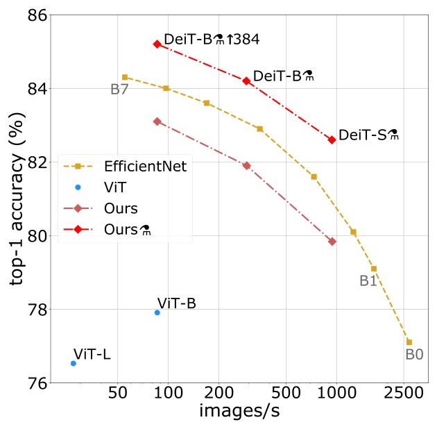
Figure 1: Throughput and accuracy on Imagenet of our methods compared to EfficientNets, trained on Imagenet1k only. The throughput is measured as the number of images processed per second on a V100 GPU. DeiT-B is identical to VIT-B, but the training is more adapted to a data-starving regime. It is learned in a few days on one machine. The symbol refers to models trained with our transformer-specific distillation. See Table 5 for details and more models.
图 1:我们的方法与 EfficientNet 在 ImageNet 上的吞吐量和精度对比,均只在 ImageNet-1k 上训练。吞吐量以一块 V100 GPU 每秒处理的图像数衡量。DeiT-B 与 ViT-B 结构相同,但训练更适合数据紧张的设定,在单机上几天就能学完。符号 ⚗ 表示用我们专为 Transformer 设计的蒸馏训练出的模型。细节及更多模型见表 5。
In this paper, we train a vision transformer on a single 8-GPU node in two to three days (53 hours of pre-training, and optionally 20 hours of fine-tuning) that is competitive with convnets having a similar number of parameters and efficiency. It uses Imagenet as the sole training set. We build upon the visual transformer architecture from Dosovitskiy et al. [15] and improvements included in the timm library [55]. With our Data-efficient image Transformers (DeiT), we report large improvements over previous results, see Figure 1. Our ablation study details the hyper-parameters and key ingredients for a successful training, such as repeated augmentation.
本文在单个 8 GPU 节点上用两到三天(预训练 53 小时,可选再微调 20 小时)训练出一个视觉 Transformer,其参数量和效率与相近的卷积网络相当。训练集只有 ImageNet。我们基于 Dosovitskiy 等人的视觉 Transformer 结构 [15],以及 timm 库中的改进 [55]。借助我们的数据高效图像 Transformer(DeiT),相对先前结果有大幅提升,见图 1。消融实验详细给出了成功训练所需的超参数和关键要素,例如重复增强。
We address another question: how to distill these models? We introduce a token-based strategy, specific to transformers and denoted by DeiT, and show that it advantageously replaces the usual distillation.
我们还讨论另一个问题:如何蒸馏这些模型?我们提出一种专门面向 Transformer、基于 token 的策略,记为 DeiT⚗,并表明它可以更好地取代通常的蒸馏。
In summary, our work makes the following contributions:
概括起来,本文的贡献如下:
- • We show that our neural networks that contains no convolutional layer can achieve competitive results against the state of the art on ImageNet with no external data. They are learned on a single node with 4 GPUs in three days[^1]. Our two new models DeiT-S and DeiT-Ti have fewer parameters and can be seen as the counterpart of ResNet-50 and ResNet-18.
[^1]: We can accelerate the learning of the larger model DeiT-B by training it on 8 GPUs in two days.
- 我们表明,不含卷积层的神经网络也能在不使用外部数据的情况下,在 ImageNet 上取得与当时最先进水平相当的结果。它们在单个 4 GPU 节点上用三天即可学成。[^1] 我们新提出的两个较小模型 DeiT-S 和 DeiT-Ti 参数更少,可以看作 ResNet-50 和 ResNet-18 的对应物。
[^1]: 更大的模型 DeiT-B 也可以加快学习:用 8 块 GPU 两天即可训练完成。
- • We introduce a new distillation procedure based on a distillation token, which plays the same role as the class token, except that it aims at reproducing the label estimated by the teacher. Both tokens interact in the transformer through attention. This transformer-specific strategy outperforms vanilla distillation by a significant margin.
- 我们提出一种基于蒸馏 token 的新蒸馏流程。它扮演的角色与类别 token 相同,只是目标改为复现教师估计的标签。两个 token 在 Transformer 里通过注意力相互作用。这种专为 Transformer 设计的策略,明显优于常规蒸馏。
- • Interestingly, with our distillation, image transformers learn more from a convnet than from another transformer with comparable performance.
- 有意思的是,采用我们的蒸馏后,图像 Transformer 从卷积网络那里学到的,比从另一个性能相当的 Transformer 那里学到的更多。
- • Our models pre-learned on Imagenet are competitive when transferred to different downstream tasks such as fine-grained classification, on several popular public benchmarks: CIFAR-10, CIFAR-100, Oxford-102 flowers, Stanford Cars and iNaturalist-18/19.
- 在 ImageNet 上预训练的模型,迁移到细粒度分类等下游任务时同样有竞争力,覆盖若干常用公开基准:CIFAR-10、CIFAR-100、Oxford-102 flowers、Stanford Cars 以及 iNaturalist-18/19。
This paper is organized as follows: we review related works in Section 2, and focus on transformers for image classification in Section 3. We introduce our distillation strategy for transformers in Section 4. The experimental section 5 provides analysis and comparisons against both convnets and recent transformers, as well as a comparative evaluation of our transformer-specific distillation. Section 6 details our training scheme. It includes an extensive ablation of our data-efficient training choices, which gives some insight on the key ingredients involved in DeiT. We conclude in Section 7.
论文结构如下:第 2 节回顾相关工作,第 3 节集中讨论用于图像分类的 Transformer。第 4 节介绍我们针对 Transformer 的蒸馏策略。第 5 节的实验提供分析,并与卷积网络及近期的 Transformer 对比,同时比较专为 Transformer 设计的蒸馏。第 6 节详细说明训练方案,包括对数据高效训练选择的系统消融,用以说明 DeiT 中的关键要素。第 7 节作结。
2 Related work
2 相关工作
Image Classification
is so core to computer vision that it is often used as a benchmark to measure progress in image understanding. Any progress usually translates to improvement in other related tasks such as detection or segmentation. Since 2012’s AlexNet [32], convnets have dominated this benchmark and have become the de facto standard. The evolution of the state of the art on the ImageNet dataset [42] reflects the progress with convolutional neural network architectures and learning [32, 44, 48, 50, 51, 57].
图像分类
在计算机视觉中如此核心,以致常被当作衡量图像理解进展的基准。这里的任何进步,通常也会转化到检测或分割等相关任务上。自 2012 年的 AlexNet [32] 以来,卷积网络主导了这一基准,并成为事实上的标准。ImageNet 数据集 [42] 上最先进水平的演变,反映了卷积网络结构与学习方法的进步 [32, 44, 48, 50, 51, 57]。
Despite several attempts to use transformers for image classification [7], until now their performance has been inferior to that of convnets. Nevertheless hybrid architectures that combine convnets and transformers, including the self-attention mechanism, have recently exhibited competitive results in image classification [56], detection [6, 28], video processing [45, 53], unsupervised object discovery [35], and unified text-vision tasks [8, 33, 37].
尽管已有若干尝试把 Transformer 用于图像分类 [7],直到当时它们的表现仍不如卷积网络。不过,把卷积网络与 Transformer(包括自注意力机制)结合起来的混合结构,最近已在图像分类 [56]、检测 [6, 28]、视频处理 [45, 53]、无监督物体发现 [35] 以及统一的文本–视觉任务 [8, 33, 37] 上展现出有竞争力的结果。
Recently Vision transformers (ViT) [15] closed the gap with the state of the art on ImageNet, without using any convolution. This performance is remarkable since convnet methods for image classification have benefited from years of tuning and optimization [22, 55]. Nevertheless, according to this study [15], a pre-training phase on a large volume of curated data is required for the learned transformer to be effective. In our paper we achieve a strong performance without requiring a large training dataset, i.e., with Imagenet1k only.
最近,视觉 Transformer(ViT)[15] 在不使用任何卷积的情况下,缩小了与 ImageNet 上最先进水平的差距。这一表现相当可观,因为用于图像分类的卷积方法已经过多年调优 [22, 55]。不过,按照该项研究 [15],要使学得的 Transformer 有效,需要先在经过整理的大规模数据上做预训练。本文在不需要大规模训练集的情况下——也就是只使用 ImageNet-1k——就达到了很强的性能。
The Transformer architecture,
introduced by Vaswani et al. [52] for machine translation are currently the reference model for all natural language processing (NLP) tasks. Many improvements of convnets for image classification are inspired by transformers. For example, Squeeze and Excitation [2], Selective Kernel [34] and Split-Attention Networks [61] exploit mechanism akin to transformers self-attention (SA) mechanism.
Transformer 结构
由 Vaswani 等人 [52] 为机器翻译提出,目前已是所有自然语言处理(NLP)任务的参考模型。图像分类里许多对卷积网络的改进,也受到 Transformer 的启发。例如 Squeeze and Excitation [2]、Selective Kernel [34] 和 Split-Attention Networks [61],都利用了与 Transformer 自注意力(SA)相近的机制。
Knowledge Distillation
(KD), introduced by Hinton et al. [24], refers to the training paradigm in which a student model leverages “soft” labels coming from a strong teacher network. This is the output vector of the teacher’s softmax function rather than just the maximum of scores, wich gives a “hard” label. Such a training improves the performance of the student model (alternatively, it can be regarded as a form of compression of the teacher model into a smaller one – the student). On the one hand the teacher’s soft labels will have a similar effect to labels smoothing [58]. On the other hand as shown by Wei et al. [54] the teacher’s supervision takes into account the effects of the data augmentation, which sometimes causes a misalignment between the real label and the image. For example, let us consider image with a “cat” label that represents a large landscape and a small cat in a corner. If the cat is no longer on the crop of the data augmentation it implicitly changes the label of the image. KD can transfer inductive biases [1] in a soft way in a student model using a teacher model where they would be incorporated in a hard way. For example, it may be useful to induce biases due to convolutions in a transformer model by using a convolutional model as teacher. In our paper we study the distillation of a transformer student by either a convnet or a transformer teacher. We introduce a new distillation procedure specific to transformers and show its superiority.
知识蒸馏
(KD)由 Hinton 等人 [24] 提出,指的是 学生 模型利用来自强 教师 网络的“软”标签来训练。这里的软标签是教师 softmax 函数的输出向量,而不只是取分数最大的“硬”标签。这样的训练会提升学生模型的表现(也可以看作把教师压缩进一个更小的学生)。一方面,教师的软标签会有类似标签平滑的效果 [58]。另一方面,如 Wei 等人 [54] 所示,教师的监督会把数据增强的影响考虑进去,而增强有时会造成真实标签与图像不对齐。例如,一张标签为“猫”的图像里是大片风景、角落里有一只小猫头;若数据增强裁到的区域里已经没有猫,图像的标签实际上就变了。KD 还可以用已经以硬方式纳入归纳偏置的教师,把这些偏置以软的方式传给学生 [1]。例如,用卷积模型当教师,有助于把卷积带来的偏置诱导进 Transformer。本文分别用卷积网络或 Transformer 当教师,来蒸馏 Transformer 学生。我们提出一种专为 Transformer 设计的新蒸馏流程,并表明它更优。
3 Vision transformer: overview
3 视觉 Transformer 概述
In this section, we briefly recall preliminaries associated with the vision transformer [15, 52], and further discuss positional encoding and resolution.
本节简要回顾与视觉 Transformer 相关的预备知识 [15, 52],并进一步讨论位置编码和分辨率。
Multi-head Self Attention layers (MSA).
The attention mechanism is based on a trainable associative memory with (key, value) vector pairs. A query vector is matched against a set of key vectors (packed together into a matrix ) using inner products. These inner products are then scaled and normalized with a softmax function to obtain weights. The output of the attention is the weighted sum of a set of value vectors (packed into ). For a sequence of query vectors (packed into ), it produces an output matrix (of size ):
多头自注意力层(MSA)。
注意力机制建立在可训练的联想记忆之上,其中存放(键,值)向量对。查询向量 与一组 个 键 向量(拼成矩阵 )做内积匹配。这些内积再缩放,并用 softmax 归一化,得到 个权重。注意力的输出是一组 个 值 向量(拼成 )的加权和。对由 个查询向量组成的序列(拼成 ),它产生一个大小为 的输出矩阵:
where the function is applied over each row of the input matrix and the term provides appropriate normalization. In [52], a Self-attention layer is proposed. Query, key and values matrices are themselves computed from a sequence of input vectors (packed into ): , , , using linear transformations with the constraint , meaning that the attention is in between all the input vectors. Finally, Multi-head self-attention layer (MSA) is defined by considering attention “heads”, ie self-attention functions applied to the input. Each head provides a sequence of size . These sequences are rearranged into a sequence that is reprojected by a linear layer into .
其中 函数沿输入矩阵的每一行作用, 提供适当的归一化。[52] 中提出了自注意力层。查询、键和值矩阵本身由 个输入向量的序列(拼成 )经线性变换得到:,,,线性变换为 ,并有约束 ,也就是注意力发生在所有输入向量之间。最后,多头自注意力层(MSA)定义为考虑 个注意力“头”,即对输入并行应用 个自注意力函数。每个头给出一个大小为 的序列。这 个序列被重排成 的序列,再由一个线性层投影回 。
Transformer block for images.
To get a full transformer block as in [52], we add a Feed-Forward Network (FFN) on top of the MSA layer. This FFN is composed of two linear layers separated by a GeLu activation [23]. The first linear layer expands the dimension from to , and the second layer reduces the dimension from back to . Both MSA and FFN are operating as residual operators thank to skip-connections, and with a layer normalization [3].
用于图像的 Transformer 块。
要得到与 [52] 中一样的完整 Transformer 块,我们在 MSA 层之上再加一个前馈网络(FFN)。这个 FFN 由两个线性层组成,中间隔着 GeLU 激活 [23]。第一个线性层把维度从 扩到 ,第二个再从 压回 。MSA 和 FFN 都借助残差连接以残差算子的方式工作,并配有层归一化 [3]。
In order to get a transformer to process images, our work builds upon the ViT model [15]. It is a simple and elegant architecture that processes input images as if they were a sequence of input tokens. The fixed-size input RGB image is decomposed into a batch of patches of a fixed size of pixels (). Each patch is projected with a linear layer that conserves its overall dimension . The transformer block described above is invariant to the order of the patch embeddings, and thus does not consider their relative position. The positional information is incorporated as fixed [52] or trainable [18] positional embeddings. They are added before the first transformer block to the patch tokens, which are then fed to the stack of transformer blocks.
为了让 Transformer 处理图像,本文建立在 ViT 模型 [15] 之上。这是一种简洁的结构,把输入图像当作一串输入 token 来处理。固定大小的输入 RGB 图像被分解成一批大小固定为 像素的 个图像块()。每个块经一个线性层投影,并保持总体维度 。上面描述的 Transformer 块对图像块嵌入的顺序不变,因而并不考虑它们的相对位置。位置信息以固定 [52] 或可训练 [18] 的位置嵌入加入。它们在第一个 Transformer 块之前加到图像块 token 上,再送入一叠 Transformer 块。
The class token
is a trainable vector, appended to the patch tokens before the first layer, that goes through the transformer layers, and is then projected with a linear layer to predict the class. This class token is inherited from NLP [14], and departs from the typical pooling layers used in computer vision to predict the class. The transformer thus process batches of tokens of dimension , of which only the class vector is used to predict the output. This architecture forces the self-attention to spread information between the patch tokens and the class token: at training time the supervision signal comes only from the class embedding, while the patch tokens are the model’s only variable input.
类别 token
是一个可训练向量,在第一层之前拼到图像块 token 后面,经过各 Transformer 层,再由一个线性层投影来预测类别。这一类别 token 继承自 NLP [14],不同于计算机视觉里通常用来预测类别的池化层。于是 Transformer 处理的是维度为 的 个 token 组成的批量,其中只有类别向量被用来预测输出。这种结构迫使自注意力在图像块 token 与类别 token 之间传递信息:训练时监督信号只来自类别嵌入,而图像块 token 是模型唯一的可变输入。
Fixing the positional encoding across resolutions.
Touvron et al. [50] show that it is desirable to use a lower training resolution and fine-tune the network at the larger resolution. This speeds up the full training and improves the accuracy under prevailing data augmentation schemes. When increasing the resolution of an input image, we keep the patch size the same, therefore the number of input patches does change. Due to the architecture of transformer blocks and the class token, the model and classifier do not need to be modified to process more tokens. In contrast, one needs to adapt the positional embeddings, because there are of them, one for each patch. Dosovitskiy et al. [15] interpolate the positional encoding when changing the resolution and demonstrate that this method works with the subsequent fine-tuning stage.
在不同分辨率下固定位置编码。
Touvron 等人 [50] 表明,用较低分辨率训练、再在更大分辨率上微调是可取的。这会加快完整训练,并在通行的数据增强方案下提高精度。提高输入图像分辨率时,我们保持图像块大小不变,因此输入块数 会改变。由于 Transformer 块和类别 token 的结构,模型和分类器不必修改就能处理更多 token。相比之下,位置嵌入需要适配,因为它们有 个,每个图像块一个。Dosovitskiy 等人 [15] 在改变分辨率时对位置编码做插值,并表明这种方法在随后的微调阶段有效。
4 Distillation through attention
4 通过注意力做蒸馏
In this section we assume we have access to a strong image classifier as a teacher model. It could be a convnet, or a mixture of classifiers. We address the question of how to learn a transformer by exploiting this teacher. As we will see in Section 5 by comparing the trade-off between accuracy and image throughput, it can be beneficial to replace a convolutional neural network by a transformer. This section covers two axes of distillation: hard distillation versus soft distillation, and classical distillation versus the distillation token.
本节假定我们已有一个很强的图像分类器作为教师模型。它可以是卷积网络,也可以是若干分类器的混合。我们关心的是如何借助这位教师来学习 Transformer。如第 5 节在精度与图像吞吐量之间的权衡比较中所示,用 Transformer 替换卷积网络可能是有益的。本节沿两个轴讨论蒸馏:硬蒸馏与软蒸馏,以及经典蒸馏与蒸馏 token。
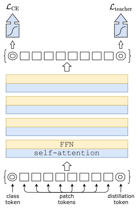
Figure 2: Our distillation procedure: we simply include a new distillation token. It interacts with the class and patch tokens through the self-attention layers. This distillation token is employed in a similar fashion as the class token, except that on output of the network its objective is to reproduce the (hard) label predicted by the teacher, instead of true label. Both the class and distillation tokens input to the transformers are learned by back-propagation.
图 2:我们的蒸馏流程:只需加入一个新的 蒸馏 token。它通过自注意力层与类别 token 和图像块 token 相互作用。这个蒸馏 token 的用法与类别 token 类似,只是在网络输出上,它的目标是复现教师预测的(硬)标签,而不是真实标签。送入 Transformer 的类别 token 和蒸馏 token 都通过反向传播来学习。
Soft distillation
[24, 54] minimizes the Kullback-Leibler divergence between the softmax of the teacher and the softmax of the student model.
软蒸馏
[24, 54] 最小化教师 softmax 与学生 softmax 之间的 Kullback-Leibler 散度。
Let be the logits of the teacher model, the logits of the student model. We denote by the temperature for the distillation, the coefficient balancing the Kullback–Leibler divergence loss () and the cross-entropy () on ground truth labels , and the softmax function. The distillation objective is
记 为教师模型的 logits, 为学生模型的 logits。 表示蒸馏温度, 是平衡 Kullback–Leibler 散度损失()与真实标签 上交叉熵()的系数, 为 softmax 函数。蒸馏目标为
Hard-label distillation.
We introduce a variant of distillation where we take the hard decision of the teacher as a true label. Let be the hard decision of the teacher, the objective associated with this hard-label distillation is:
硬标签蒸馏。
我们引入一种蒸馏变体:把教师的硬判决当作真实标签。记 为教师的硬判决,与这种硬标签蒸馏对应的目标是:
For a given image, the hard label associated with the teacher may change depending on the specific data augmentation. We will see that this choice is better than the traditional one, while being parameter-free and conceptually simpler: The teacher prediction plays the same role as the true label .
对给定图像,与教师对应的硬标签可能随具体的数据增强而改变。我们会看到,这一选择优于传统做法,而且不引入额外参数,概念上也更简单:教师预测 扮演的角色与真实标签 相同。
Note also that the hard labels can also be converted into soft labels with label smoothing [47], where the true label is considered to have a probability of , and the remaining is shared across the remaining classes. We fix this parameter to in our all experiments that use true labels.
还需要指出,硬标签也可以用标签平滑 [47] 转成软标签,其中真实标签的概率视为 ,剩下的 分给其余类别。在所有使用真实标签的实验中,我们把该参数固定为 。
Distillation token.
We now focus on our proposal, which is illustrated in Figure 2. We add a new token, the distillation token, to the initial embeddings (patches and class token). Our distillation token is used similarly as the class token: it interacts with other embeddings through self-attention, and is output by the network after the last layer. Its target objective is given by the distillation component of the loss. The distillation embedding allows our model to learn from the output of the teacher, as in a regular distillation, while remaining complementary to the class embedding.
蒸馏 token。
下面集中讨论我们的方案,如图 2 所示。我们在初始嵌入(图像块和类别 token)中加入一个新的 token,即蒸馏 token。它的用法与类别 token 类似:通过自注意力与其他嵌入相互作用,并在最后一层由网络输出。它的目标由损失中的蒸馏项给出。蒸馏嵌入使我们的模型能像常规蒸馏那样向教师的输出学习,同时又与类别嵌入保持互补。
Interestingly, we observe that the learned class and distillation tokens converge towards different vectors: the average cosine similarity between these tokens equal to 0.06. As the class and distillation embeddings are computed at each layer, they gradually become more similar through the network, all the way through the last layer at which their similarity is high (cos=0.93), but still lower than 1. This is expected since as they aim at producing targets that are similar but not identical.
有意思的是,我们观察到学得的类别 token 与蒸馏 token 收敛到不同的向量:这些 token 之间的平均余弦相似度等于 0.06。由于类别嵌入和蒸馏嵌入在每一层都会被计算,它们沿网络逐渐变得更相似,直到最后一层相似度已经很高(),但仍低于 1。这是预期之中的,因为它们要产生的目标相近但不相同。
We verified that our distillation token adds something to the model, compared to simply adding an additional class token associated with the same target label: instead of a teacher pseudo-label, we experimented with a transformer with two class tokens. Even if we initialize them randomly and independently, during training they converge towards the same vector (cos=0.999), and the output embedding are also quasi-identical. This additional class token does not bring anything to the classification performance. In contrast, our distillation strategy provides a significant improvement over a vanilla distillation baseline, as validated by our experiments in Section 5.2.
我们核验了蒸馏 token 确实给模型带来了额外作用,而不是简单地再加一个对准同一目标标签的类别 token:我们试过不用教师伪标签,而是给 Transformer 两个类别 token。即便把它们随机、独立地初始化,训练中它们也会收敛到同一个向量(),输出嵌入也几乎相同。这个额外的类别 token 对分类性能没有帮助。相比之下,我们的蒸馏策略相对常规蒸馏基线有明显提升,第 5.2 节的实验验证了这一点。
Fine-tuning with distillation.
We use both the true label and teacher prediction during the fine-tuning stage at higher resolution. We use a teacher with the same target resolution, typically obtained from the lower-resolution teacher by the method of Touvron et al [50]. We have also tested with true labels only but this reduces the benefit of the teacher and leads to a lower performance.
带蒸馏的微调。
在更高分辨率的微调阶段,我们同时使用真实标签和教师预测。教师采用相同的目标分辨率,通常由较低分辨率的教师按 Touvron 等人的方法 [50] 得到。我们也试过只用真实标签,但这会削弱教师的收益,导致性能下降。
Classification with our approach: joint classifiers.
At test time, both the class or the distillation embeddings produced by the transformer are associated with linear classifiers and able to infer the image label. Yet our referent method is the late fusion of these two separate heads, for which we add the softmax output by the two classifiers to make the prediction. We evaluate these three options in Section 5.
用我们的方法做分类:联合分类器。
测试时,Transformer 产生的类别嵌入和蒸馏嵌入各自对应线性分类器,都能推断图像标签。不过我们的基准方法是这两个独立头的晚期融合:把两个分类器输出的 softmax 相加再做预测。第 5 节评估了这三种选项。
5 Experiments
5 实验
This section presents a few analytical experiments and results. We first discuss our distillation strategy. Then we comparatively analyze the efficiency and accuracy of convnets and vision transformers.
本节给出若干分析实验和结果。我们先讨论蒸馏策略,再比较卷积网络与视觉 Transformer 的效率和精度。
5.1 Transformer models
5.1 Transformer 模型
As mentioned earlier, our architecture design is identical to the one proposed by Dosovitskiy et al. [15] with no convolutions. Our only differences are the training strategies, and the distillation token. Also we do not use a MLP head for the pre-training but only a linear classifier. To avoid any confusion, we refer to the results obtained in the prior work by ViT, and prefix ours by DeiT. If not specified, DeiT refers to our referent model DeiT-B, which has the same architecture as ViT-B. When we fine-tune DeiT at a larger resolution, we append the resulting operating resolution at the end, e.g, DeiT-B384. Last, when using our distillation procedure, we identify it with an alembic sign as DeiT.
如前所述,我们的结构设计与 Dosovitskiy 等人 [15] 提出的相同,不含卷积。唯一的差别是训练策略,以及蒸馏 token。此外,预训练时我们不用 MLP 头,只用线性分类器。为避免混淆,先前工作得到的结果记为 ViT,我们的结果以 DeiT 为前缀。若未特别说明,DeiT 指基准模型 DeiT-B,其结构与 ViT-B 相同。若在更大分辨率上微调 DeiT,我们把最终工作分辨率附在名称后面,例如 DeiT-B384。最后,采用我们的蒸馏流程时,用蒸馏符号记为 DeiT⚗。
The parameters of ViT-B (and therefore of DeiT-B) are fixed as , and . We introduce two smaller models, namely DeiT-S and DeiT-Ti, for which we change the number of heads, keeping fixed. Table 1 summarizes the models that we consider in our paper.
ViT-B(因而也是 DeiT-B)的参数固定为 ,,。我们另外引入两个更小的模型 DeiT-S 和 DeiT-Ti,改变头数并保持 不变。表 1 汇总了本文考虑的模型。
| Model | ViT model | embedding | #heads | #layers | #params | training | throughput |
|---|---|---|---|---|---|---|---|
| dimension | resolution | (im/sec) | |||||
| DeiT-Ti | N/A | 0192 | 03 | 12 | 005M | 224 | 2536 |
| DeiT-S | N/A | 0384 | 06 | 12 | 022M | 224 | 0940 |
| DeiT-B | ViT-B | 0768 | 12 | 12 | 086M | 224 | 0292 |
Table 1: Variants of our DeiT architecture. The larger model, DeiT-B, has the same architecture as the ViT-B [15]. The only parameters that vary across models are the embedding dimension and the number of heads, and we keep the dimension per head constant (equal to 64). Smaller models have a lower parameter count, and a faster throughput. The throughput is measured for images at resolution 224224.
| 模型 | ViT 模型 | 嵌入 | 头数 | 层数 | 参数量 | 训练 | 吞吐量 |
|---|---|---|---|---|---|---|---|
| 维度 | 分辨率 | (图像/秒) | |||||
| DeiT-Ti | 无 | 192 | 3 | 12 | 5M | 224 | 2536 |
| DeiT-S | 无 | 384 | 6 | 12 | 22M | 224 | 940 |
| DeiT-B | ViT-B | 768 | 12 | 12 | 86M | 224 | 292 |
表 1:我们的 DeiT 结构变体。较大的模型 DeiT-B 与 ViT-B [15] 结构相同。各模型之间变化的参数只有嵌入维度和头数,我们保持每个头的维度不变(等于 64)。较小的模型参数更少,吞吐量更快。吞吐量在分辨率 的图像上测量。
5.2 Distillation
5.2 蒸馏
Our distillation method produces a vision transformer that becomes on par with the best convnets in terms of the trade-off between accuracy and throughput, see Table 5. Interestingly, the distilled model outperforms its teacher in terms of the trade-off between accuracy and throughput. Our best model on ImageNet-1k is 85.2% top-1 accuracy outperforms the best Vit-B model pre-trained on JFT-300M at resolution 384 (84.15%). For reference, the current state of the art of 88.55% achieved with extra training data was obtained by the ViT-H model (600M parameters) trained on JFT-300M at resolution 512. Hereafter we provide several analysis and observations.
我们的蒸馏方法得到的视觉 Transformer,在精度与吞吐量的权衡上已经能与最好的卷积网络相当,见表 5。有意思的是,蒸馏后的模型在这一权衡上还超过了它的教师。我们在 ImageNet-1k 上最好的模型达到 85.2% 的 top-1 精度,超过了在 JFT-300M 上预训练、分辨率为 384 的最佳 ViT-B 模型(84.15%)。作为参照,当时利用额外训练数据得到的最先进水平是 88.55%,由在 JFT-300M 上、以分辨率 512 训练的 ViT-H 模型(6 亿参数)取得。下面给出若干分析和观察。
Convnets teachers.
We have observed that using a convnet teacher gives better performance than using a transformer. Table 2 compares distillation results with different teacher architectures. The fact that the convnet is a better teacher is probably due to the inductive bias inherited by the transformers through distillation, as explained in Abnar et al. [1]. In all of our subsequent distillation experiments the default teacher is a RegNetY-16GF [40] (84M parameters) that we trained with the same data and same data-augmentation as DeiT. This teacher reaches top-1 accuracy on ImageNet.
卷积网络教师。
我们观察到,用卷积网络当教师,效果好于用 Transformer。表 2 比较了不同教师结构下的蒸馏结果。卷积网络是更好的教师,很可能是因为 Transformer 通过蒸馏继承了归纳偏置,正如 Abnar 等人 [1] 所解释的。在随后所有蒸馏实验中,默认教师是一个 RegNetY-16GF [40](8400 万参数),我们用与 DeiT 相同的数据和数据增强来训练它。这位教师在 ImageNet 上达到 的 top-1 精度。
| Teacher | Student: DeiT-B | ||
|---|---|---|---|
| Models | acc. | pretrain | 384 |
| DeiT-B | 81.8 | 81.9 | 83.1 |
| RegNetY-4GF | 80.0 | 82.7 | 83.6 |
| RegNetY-8GF | 81.7 | 82.7 | 83.8 |
| RegNetY-12GF | 82.4 | 83.1 | 84.1 |
| RegNetY-16GF | 82.9 | 83.1 | 84.2 |
Table 2: We compare on ImageNet [42] the performance (top-1 acc., %) of the student as a function of the teacher model used for distillation.
| 教师 | 学生:DeiT-B | ||
|---|---|---|---|
| 模型 | 精度 | 预训练 | 384 |
| DeiT-B | 81.8 | 81.9 | 83.1 |
| RegNetY-4GF | 80.0 | 82.7 | 83.6 |
| RegNetY-8GF | 81.7 | 82.7 | 83.8 |
| RegNetY-12GF | 82.4 | 83.1 | 84.1 |
| RegNetY-16GF | 82.9 | 83.1 | 84.2 |
表 2:我们在 ImageNet [42] 上比较学生的表现(top-1 精度,%)如何随用于蒸馏的教师模型变化。
Comparison of distillation methods.
We compare the performance of different distillation strategies in Table 3. Hard distillation significantly outperforms soft distillation for transformers, even when using only a class token: hard distillation reaches 83.0% at resolution 224224, compared to the soft distillation accuracy of 81.8%. Our distillation strategy from Section 4 further improves the performance, showing that the two tokens provide complementary information useful for classification: the classifier on the two tokens is significantly better than the independent class and distillation classifiers, which by themselves already outperform the distillation baseline.
蒸馏方法的比较。
我们在表 3 中比较不同蒸馏策略的表现。对 Transformer 而言,硬蒸馏明显优于软蒸馏,即便只用类别 token:硬蒸馏在分辨率 上达到 83.0%,而软蒸馏的精度是 81.8%。第 4 节的蒸馏策略还能进一步提高表现,说明两个 token 提供了对分类有用的互补信息:同时使用两个 token 的分类器,明显好于各自独立的类别分类器和蒸馏分类器,而后两者本身已经超过蒸馏基线。
The distillation token gives slightly better results than the class token. It is also more correlated to the convnets prediction. This difference in performance is probably due to the fact that it benefits more from the inductive bias of convnets. We give more details and an analysis in the next paragraph. The distillation token has an undeniable advantage for the initial training.
蒸馏 token 的结果略好于类别 token。它与卷积网络预测的相关性也更高。这一性能差异,很可能是因为它更多地受益于卷积网络的归纳偏置。下一小节给出更多细节和分析。蒸馏 token 在初始训练中具有明显优势。
Agreement with the teacher & inductive bias?
As discussed above, the architecture of the teacher has an important impact. Does it inherit existing inductive bias that would facilitate the training? While we believe it difficult to formally answer this question, we analyze in Table 4 the decision agreement between the convnet teacher, our image transformer DeiT learned from labels only, and our transformer DeiT.
与教师的一致性及归纳偏置?
如上所述,教师的结构有重要影响。它是否会继承已有的归纳偏置,从而方便训练?我们觉得很难形式化地回答这个问题,但在表 4 中分析了卷积网络教师、只从标签学习的图像 Transformer DeiT,以及我们的蒸馏 Transformer DeiT⚗ 之间的判决一致性。
Our distilled model is more correlated to the convnet than with a transformer learned from scratch. As to be expected, the classifier associated with the distillation embedding is closer to the convnet that the one associated with the class embedding, and conversely the one associated with the class embedding is more similar to DeiT learned without distillation. Unsurprisingly, the joint class+distil classifier offers a middle ground.
我们的蒸馏模型与卷积网络的相关性,高于它与从零训练的 Transformer 的相关性。正如所料,与蒸馏嵌入对应的分类器更接近卷积网络,而与类别嵌入对应的分类器更接近未做蒸馏的 DeiT。毫不意外,联合的类别+蒸馏分类器介于两者之间。
| Supervision | ImageNet top-1 (%) | |||||
|---|---|---|---|---|---|---|
| method | label | teacher | Ti 224 | S 224 | B 224 | B384 |
| DeiT– no distillation | ✓ | ✗ | 72.2 | 79.8 | 81.8 | 83.1 |
| DeiT– usual distillation | ✗ | soft | 72.2 | 79.8 | 81.8 | 83.2 |
| DeiT– hard distillation | ✗ | hard | 74.3 | 80.9 | 83.0 | 84.0 |
| DeiT: class embedding | ✓ | hard | 73.9 | 80.9 | 83.0 | 84.2 |
| DeiT: distil. embedding | ✓ | hard | 74.6 | 81.1 | 83.1 | 84.4 |
| DeiT: class+distillation | ✓ | hard | 74.5 | 81.2 | 83.4 | 84.5 |
Table 3: Distillation experiments on Imagenet with DeiT, 300 epochs of pre-training. We report the results for our new distillation method in the last three rows. We separately report the performance when classifying with only one of the class or distillation embeddings, and then with a classifier taking both of them as input. In the last row (class+distillation), the result correspond to the late fusion of the class and distillation classifiers.
| 监督 | ImageNet top-1(%) | |||||
|---|---|---|---|---|---|---|
| 方法 | 标签 | 教师 | Ti 224 | S 224 | B 224 | B384 |
| DeiT– 无蒸馏 | ✓ | ✗ | 72.2 | 79.8 | 81.8 | 83.1 |
| DeiT– 常规蒸馏 | ✗ | 软 | 72.2 | 79.8 | 81.8 | 83.2 |
| DeiT– 硬蒸馏 | ✗ | 硬 | 74.3 | 80.9 | 83.0 | 84.0 |
| DeiT⚗:类别嵌入 | ✓ | 硬 | 73.9 | 80.9 | 83.0 | 84.2 |
| DeiT⚗:蒸馏嵌入 | ✓ | 硬 | 74.6 | 81.1 | 83.1 | 84.4 |
| DeiT⚗:类别+蒸馏 | ✓ | 硬 | 74.5 | 81.2 | 83.4 | 84.5 |
表 3:在 ImageNet 上用 DeiT 做蒸馏实验,预训练 300 个周期。最后三行报告我们的新蒸馏方法。我们分别报告只用类别嵌入或只用蒸馏嵌入分类时的表现,然后再报告以两者为输入的分类器。最后一行(类别+蒸馏)的结果对应类别分类器与蒸馏分类器的晚期融合。
Number of epochs.
Increasing the number of epochs significantly improves the performance of training with distillation, see Figure 3. With 300 epochs, our distilled network DeiT-B is already better than DeiT-B. But while for the latter the performance saturates with longer schedules, our distilled network clearly benefits from a longer training time.
训练周期数。
增加周期数会显著提高带蒸馏训练的表现,见图 3。用 300 个周期时,我们的蒸馏网络 DeiT-B⚗ 已经优于 DeiT-B。但对后者而言,更长的训练日程会使性能趋于饱和,而我们的蒸馏网络则明显受益于更长的训练时间。
| groundtruth | no distillation | DeiT student (of the convnet) | ||||
|---|---|---|---|---|---|---|
| convnet | DeiT | class | distillation | DeiT | ||
| groundtruth | 0.000 | 0.171 | 0.182 | 0.170 | 0.169 | 0.166 |
| convnet (RegNetY) | 0.171 | 0.000 | 0.133 | 0.112 | 0.100 | 0.102 |
| DeiT | 0.182 | 0.133 | 0.000 | 0.109 | 0.110 | 0.107 |
| DeiT– class only | 0.170 | 0.112 | 0.109 | 0.000 | 0.050 | 0.033 |
| DeiT– distil. only | 0.169 | 0.100 | 0.110 | 0.050 | 0.000 | 0.019 |
| DeiT– class+distil. | 0.166 | 0.102 | 0.107 | 0.033 | 0.019 | 0.000 |
Table 4: Disagreement analysis between convnet, image transformers and distillated transformers: We report the fraction of sample classified differently for all classifier pairs, i.e., the rate of different decisions. We include two models without distillation (a RegNetY and DeiT-B), so that we can compare how our distilled models and classification heads are correlated to these teachers.
| 真实标签 | 无蒸馏 | 卷积网络的 DeiT 学生 | ||||
|---|---|---|---|---|---|---|
| 卷积网络 | DeiT | 类别 | 蒸馏 | DeiT⚗ | ||
| 真实标签 | 0.000 | 0.171 | 0.182 | 0.170 | 0.169 | 0.166 |
| 卷积网络(RegNetY) | 0.171 | 0.000 | 0.133 | 0.112 | 0.100 | 0.102 |
| DeiT | 0.182 | 0.133 | 0.000 | 0.109 | 0.110 | 0.107 |
| DeiT⚗– 仅类别 | 0.170 | 0.112 | 0.109 | 0.000 | 0.050 | 0.033 |
| DeiT⚗– 仅蒸馏 | 0.169 | 0.100 | 0.110 | 0.050 | 0.000 | 0.019 |
| DeiT⚗– 类别+蒸馏 | 0.166 | 0.102 | 0.107 | 0.033 | 0.019 | 0.000 |
表 4:卷积网络、图像 Transformer 与蒸馏后 Transformer 之间的不一致分析:我们报告所有分类器两两之间分类结果不同的样本比例,也就是判决不同的比率。我们纳入两个未做蒸馏的模型(一个 RegNetY 和一个 DeiT-B),以便比较我们的蒸馏模型及分类头与这些教师的相关程度。
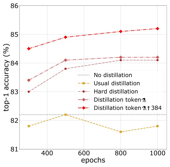
Figure 3: Distillation on ImageNet [42] with DeiT-B: performance as a function of the number of training epochs. We provide the performance without distillation (horizontal dotted line) as it saturates after 400 epochs.
图 3:在 ImageNet [42] 上用 DeiT-B 做蒸馏:表现随训练周期数的变化。我们同时给出不做蒸馏时的表现(水平虚线),它在 400 个周期之后趋于饱和。
5.3 Efficiency vs accuracy: a comparative study with convnets
5.3 效率与精度:与卷积网络的对比研究
In the literature, the image classificaton methods are often compared as a compromise between accuracy and another criterion, such as FLOPs, number of parameters, size of the network, etc.
文献中,图像分类方法常常被放在精度与另一项指标之间权衡,例如浮点运算量、参数量、网络大小等。
We focus in Figure 1 on the tradeoff between the throughput (images processed per second) and the top-1 classification accuracy on ImageNet. We focus on the popular state-of-the-art EfficientNet convnet, which has benefited from years of research on convnets and was optimized by architecture search on the ImageNet validation set.
我们在图 1 中关注吞吐量(每秒处理的图像数)与 ImageNet 上 top-1 分类精度之间的权衡。重点对照当时流行、也代表最先进水平的 EfficientNet 卷积网络——它受益于多年的卷积网络研究,并在 ImageNet 验证集上用结构搜索做过优化。
Our method DeiT is slightly below EfficientNet, which shows that we have almost closed the gap between vision transformers and convnets when training with Imagenet only. These results are a major improvement (+6.3% top-1 in a comparable setting) over previous ViT models trained on Imagenet1k only [15]. Furthermore, when DeiT benefits from the distillation from a relatively weaker RegNetY to produce DeiT, it outperforms EfficientNet. It also outperforms by 1% (top-1 acc.) the Vit-B model pre-trained on JFT300M at resolution 384 (85.2% vs 84.15%), while being significantly faster to train.
我们的方法 DeiT 略低于 EfficientNet,说明在只使用 ImageNet 训练时,我们已经几乎补上了视觉 Transformer 与卷积网络之间的差距。这些结果相对先前只在 ImageNet-1k 上训练的 ViT 模型 [15] 有大幅提升(在可比设定下 top-1 提高 6.3%)。进一步地,当 DeiT 从一个相对更弱的 RegNetY 蒸馏得到 DeiT⚗ 之后,它超过了 EfficientNet。它还比在 JFT-300M 上预训练、分辨率为 384 的 ViT-B 高出 1 个百分点(top-1 精度 85.2% 对 84.15%),同时训练明显更快。
Table 5 reports the numerical results in more details and additional evaluations on ImageNet V2 and ImageNet Real, that have a test set distinct from the ImageNet validation, which reduces overfitting on the validation set. Our results show that DeiT-B and DeiT-B 384 outperform, by some margin, the state of the art on the trade-off between accuracy and inference time on GPU.
表 5 给出更详细的数值结果,以及在 ImageNet V2 和 ImageNet Real 上的额外评估。这两个集合的测试集与 ImageNet 验证集不同,从而减轻了在验证集上过拟合的问题。结果表明,DeiT-B 和 DeiT-B 384 在精度与 GPU 推理时间的权衡上,以一定幅度超过了当时的最先进水平。
| image | throughput | ImNet | Real | V2 | ||
|---|---|---|---|---|---|---|
| Network | #param. | size | (image/s) | top-1 | top-1 | top-1 |
| Convnets | ||||||
| ResNet-18 [21] | 12M | 4458.4 | 69.8 | 77.3 | 57.1 | |
| ResNet-50 [21] | 25M | 1226.1 | 76.2 | 82.5 | 63.3 | |
| ResNet-101 [21] | 45M | 0753.6 | 77.4 | 83.7 | 65.7 | |
| ResNet-152 [21] | 60M | 0526.4 | 78.3 | 84.1 | 67.0 | |
| RegNetY-4GF [40] | 21M | 1156.7 | 80.0 | 86.4 | 69.4 | |
| RegNetY-8GF [40] | 39M | 0591.6 | 81.7 | 87.4 | 70.8 | |
| RegNetY-16GF [40] | 84M | 0334.7 | 82.9 | 88.1 | 72.4 | |
| EfficientNet-B0 [48] | 5M | 2694.3 | 77.1 | 83.5 | 64.3 | |
| EfficientNet-B1 [48] | 8M | 1662.5 | 79.1 | 84.9 | 66.9 | |
| EfficientNet-B2 [48] | 9M | 1255.7 | 80.1 | 85.9 | 68.8 | |
| EfficientNet-B3 [48] | 12M | 0732.1 | 81.6 | 86.8 | 70.6 | |
| EfficientNet-B4 [48] | 19M | 0349.4 | 82.9 | 88.0 | 72.3 | |
| EfficientNet-B5 [48] | 30M | 0169.1 | 83.6 | 88.3 | 73.6 | |
| EfficientNet-B6 [48] | 43M | 0096.9 | 84.0 | 88.8 | 73.9 | |
| EfficientNet-B7 [48] | 66M | 0055.1 | 84.3 | _ | _ | |
| EfficientNet-B5 RA [12] | 30M | 0096.9 | 83.7 | _ | _ | |
| EfficientNet-B7 RA [12] | 66M | 0055.1 | 84.7 | _ | _ | |
| KDforAA-B8 | 87M | 0025.2 | 85.8 | _ | _ | |
| Transformers | ||||||
| ViT-B/16 [15] | 86M | 0085.9 | 77.9 | 83.6 | _ | |
| ViT-L/16 [15] | 307M | 0027.3 | 76.5 | 82.2 | _ | |
| DeiT-Ti | 5M | 2536.5 | 72.2 | 80.1 | 60.4 | |
| DeiT-S | 22M | 0940.4 | 79.8 | 85.7 | 68.5 | |
| DeiT-B | 86M | 0292.3 | 81.8 | 86.7 | 71.5 | |
| DeiT-B384 | 86M | 0085.9 | 83.1 | 87.7 | 72.4 | |
| DeiT-Ti | 6M | 2529.5 | 74.5 | 82.1 | 62.9 | |
| DeiT-S | 22M | 0936.2 | 81.2 | 86.8 | 70.0 | |
| DeiT-B | 87M | 0290.9 | 83.4 | 88.3 | 73.2 | |
| DeiT-Ti/ 1000 epochs | 6M | 2529.5 | 76.6 | 83.9 | 65.4 | |
| DeiT-S/ 1000 epochs | 22M | 0936.2 | 82.6 | 87.8 | 71.7 | |
| DeiT-B/ 1000 epochs | 87M | 0290.9 | 84.2 | 88.7 | 73.9 | |
| DeiT-B 384 | 87M | 0085.8 | 84.5 | 89.0 | 74.8 | |
| DeiT-B 384 / 1000 epochs | 87M | 0085.8 | 85.2 | 89.3 | 75.2 |
Table 5: Throughput on and accuracy on Imagenet [42], Imagenet Real [5] and Imagenet V2 matched frequency [41] of DeiT and of several state-of-the-art convnets, for models trained with no external data. The throughput is measured as the number of images that we can process per second on one 16GB V100 GPU. For each model we take the largest possible batch size for the usual resolution of the model and calculate the average time over 30 runs to process that batch. With that we calculate the number of images processed per second. Throughput can vary according to the implementation: for a direct comparison and in order to be as fair as possible, we use for each model the definition in the same GitHub [55] repository. Regnet optimized with a similar optimization procedure as ours, which boosts the results. These networks serve as teachers when we use our distillation strategy.
| 图像 | 吞吐量 | ImNet | Real | V2 | ||
|---|---|---|---|---|---|---|
| 网络 | 参数量 | 尺寸 | (图像/秒) | top-1 | top-1 | top-1 |
| 卷积网络 | ||||||
| ResNet-18 [21] | 12M | 4458.4 | 69.8 | 77.3 | 57.1 | |
| ResNet-50 [21] | 25M | 1226.1 | 76.2 | 82.5 | 63.3 | |
| ResNet-101 [21] | 45M | 753.6 | 77.4 | 83.7 | 65.7 | |
| ResNet-152 [21] | 60M | 526.4 | 78.3 | 84.1 | 67.0 | |
| RegNetY-4GF [40] | 21M | 1156.7 | 80.0 | 86.4 | 69.4 | |
| RegNetY-8GF [40] | 39M | 591.6 | 81.7 | 87.4 | 70.8 | |
| RegNetY-16GF [40] | 84M | 334.7 | 82.9 | 88.1 | 72.4 | |
| EfficientNet-B0 [48] | 5M | 2694.3 | 77.1 | 83.5 | 64.3 | |
| EfficientNet-B1 [48] | 8M | 1662.5 | 79.1 | 84.9 | 66.9 | |
| EfficientNet-B2 [48] | 9M | 1255.7 | 80.1 | 85.9 | 68.8 | |
| EfficientNet-B3 [48] | 12M | 732.1 | 81.6 | 86.8 | 70.6 | |
| EfficientNet-B4 [48] | 19M | 349.4 | 82.9 | 88.0 | 72.3 | |
| EfficientNet-B5 [48] | 30M | 169.1 | 83.6 | 88.3 | 73.6 | |
| EfficientNet-B6 [48] | 43M | 96.9 | 84.0 | 88.8 | 73.9 | |
| EfficientNet-B7 [48] | 66M | 55.1 | 84.3 | _ | _ | |
| EfficientNet-B5 RA [12] | 30M | 96.9 | 83.7 | _ | _ | |
| EfficientNet-B7 RA [12] | 66M | 55.1 | 84.7 | _ | _ | |
| KDforAA-B8 | 87M | 25.2 | 85.8 | _ | _ | |
| Transformer | ||||||
| ViT-B/16 [15] | 86M | 85.9 | 77.9 | 83.6 | _ | |
| ViT-L/16 [15] | 307M | 27.3 | 76.5 | 82.2 | _ | |
| DeiT-Ti | 5M | 2536.5 | 72.2 | 80.1 | 60.4 | |
| DeiT-S | 22M | 940.4 | 79.8 | 85.7 | 68.5 | |
| DeiT-B | 86M | 292.3 | 81.8 | 86.7 | 71.5 | |
| DeiT-B384 | 86M | 85.9 | 83.1 | 87.7 | 72.4 | |
| DeiT⚗-Ti | 6M | 2529.5 | 74.5 | 82.1 | 62.9 | |
| DeiT⚗-S | 22M | 936.2 | 81.2 | 86.8 | 70.0 | |
| DeiT⚗-B | 87M | 290.9 | 83.4 | 88.3 | 73.2 | |
| DeiT⚗-Ti / 1000 周期 | 6M | 2529.5 | 76.6 | 83.9 | 65.4 | |
| DeiT⚗-S / 1000 周期 | 22M | 936.2 | 82.6 | 87.8 | 71.7 | |
| DeiT⚗-B / 1000 周期 | 87M | 290.9 | 84.2 | 88.7 | 73.9 | |
| DeiT⚗-B 384 | 87M | 85.8 | 84.5 | 89.0 | 74.8 | |
| DeiT⚗-B 384 / 1000 周期 | 87M | 85.8 | 85.2 | 89.3 | 75.2 |
表 5:在不使用外部数据训练的设定下,DeiT 与若干当时最先进的卷积网络在 ImageNet [42]、ImageNet Real [5] 以及 ImageNet V2 matched frequency [41] 上的吞吐量和精度。吞吐量以一块 16GB V100 GPU 每秒能处理的图像数衡量。对每个模型,我们在该模型常用分辨率下取尽可能大的批量,将处理该批量的时间对 30 次运行取平均,再据此计算每秒处理的图像数。吞吐量会因实现而异:为了直接比较并尽量公平,我们对每个模型都采用同一 GitHub 仓库 [55] 中的定义。:用与我们类似的优化流程训练的 RegNet,结果因此提高。采用蒸馏策略时,这些网络充当教师。
5.4 Transfer learning: Performance on downstream tasks
5.4 迁移学习:在下游任务上的表现
Although DeiT perform very well on ImageNet it is important to evaluate them on other datasets with transfer learning in order to measure the power of generalization of DeiT. We evaluated this on transfer learning tasks by fine-tuning on the datasets in Table 6. Table 7 compares DeiT transfer learning results to those of ViT [15] and state of the art convolutional architectures [48]. DeiT is on par with competitive convnet models, which is in line with our previous conclusion on ImageNet.
尽管 DeiT 在 ImageNet 上表现很好,仍有必要在其他数据集上用迁移学习来评估,以衡量 DeiT 的泛化能力。我们在表 6 所列数据集上做微调,以此评估迁移学习。表 7 将 DeiT 的迁移结果与 ViT [15] 以及当时最先进的卷积结构 [48] 相比较。DeiT 与有竞争力的卷积模型处于同一水平,这与我们先前在 ImageNet 上的结论一致。
| Dataset | Train size | Test size | #classes |
|---|---|---|---|
| ImageNet [42] | 1,281,167 | 50,000 | 1000 |
| iNaturalist 2018 [26] | 437,513 | 24,426 | 8,142 |
| iNaturalist 2019 [27] | 265,240 | 3,003 | 1,010 |
| Flowers-102 [38] | 2,040 | 6,149 | 102 |
| Stanford Cars [30] | 8,144 | 8,041 | 196 |
| CIFAR-100 [31] | 50,000 | 10,000 | 100 |
| CIFAR-10 [31] | 50,000 | 10,000 | 10 |
Table 6: Datasets used for our different tasks.
| 数据集 | 训练集大小 | 测试集大小 | 类别数 |
|---|---|---|---|
| ImageNet [42] | 1,281,167 | 50,000 | 1000 |
| iNaturalist 2018 [26] | 437,513 | 24,426 | 8,142 |
| iNaturalist 2019 [27] | 265,240 | 3,003 | 1,010 |
| Flowers-102 [38] | 2,040 | 6,149 | 102 |
| Stanford Cars [30] | 8,144 | 8,041 | 196 |
| CIFAR-100 [31] | 50,000 | 10,000 | 100 |
| CIFAR-10 [31] | 50,000 | 10,000 | 10 |
表 6:各任务所用的数据集。
| Model | ImageNet | CIFAR-10 | CIFAR-100 | Flowers | Cars | iNat-18 | iNat-19 | im/sec |
|---|---|---|---|---|---|---|---|---|
| Grafit ResNet-50 [49] | 79.6 | _ | _ | 98.2 | 92.5 | 69.8 | 75.9 | 1226.1 |
| Grafit RegNetY-8GF [49] | _ | _ | _ | 99.0 | 94.0 | 76.8 | 80.0 | 591.6 |
| ResNet-152 [10] | _ | _ | _ | _ | _ | 69.1 | _ | 526.3 |
| EfficientNet-B7 [48] | 84.3 | 98.9 | 91.7 | 98.8 | 94.7 | _ | _ | 55.1 |
| ViT-B/32 [15] | 73.4 | 97.8 | 86.3 | 85.4 | _ | _ | _ | 394.5 |
| ViT-B/16 [15] | 77.9 | 98.1 | 87.1 | 89.5 | _ | _ | _ | 85.9 |
| ViT-L/32 [15] | 71.2 | 97.9 | 87.1 | 86.4 | _ | _ | _ | 124.1 |
| ViT-L/16 [15] | 76.5 | 97.9 | 86.4 | 89.7 | _ | _ | _ | 27.3 |
| DeiT-B | 81.8 | 99.1 | 90.8 | 98.4 | 92.1 | 73.2 | 77.7 | 292.3 |
| DeiT-B384 | 83.1 | 99.1 | 90.8 | 98.5 | 93.3 | 79.5 | 81.4 | 085.9 |
| DeiT-B | 83.4 | 99.1 | 91.3 | 98.8 | 92.9 | 73.7 | 78.4 | 290.9 |
| DeiT-B 384 | 84.4 | 99.2 | 91.4 | 98.9 | 93.9 | 80.1 | 83.0 | 085.9 |
Table 7: We compare Transformers based models on different transfer learning task with ImageNet pre-training. We also report results with convolutional architectures for reference.
| 模型 | ImageNet | CIFAR-10 | CIFAR-100 | Flowers | Cars | iNat-18 | iNat-19 | 图像/秒 |
|---|---|---|---|---|---|---|---|---|
| Grafit ResNet-50 [49] | 79.6 | _ | _ | 98.2 | 92.5 | 69.8 | 75.9 | 1226.1 |
| Grafit RegNetY-8GF [49] | _ | _ | _ | 99.0 | 94.0 | 76.8 | 80.0 | 591.6 |
| ResNet-152 [10] | _ | _ | _ | _ | _ | 69.1 | _ | 526.3 |
| EfficientNet-B7 [48] | 84.3 | 98.9 | 91.7 | 98.8 | 94.7 | _ | _ | 55.1 |
| ViT-B/32 [15] | 73.4 | 97.8 | 86.3 | 85.4 | _ | _ | _ | 394.5 |
| ViT-B/16 [15] | 77.9 | 98.1 | 87.1 | 89.5 | _ | _ | _ | 85.9 |
| ViT-L/32 [15] | 71.2 | 97.9 | 87.1 | 86.4 | _ | _ | _ | 124.1 |
| ViT-L/16 [15] | 76.5 | 97.9 | 86.4 | 89.7 | _ | _ | _ | 27.3 |
| DeiT-B | 81.8 | 99.1 | 90.8 | 98.4 | 92.1 | 73.2 | 77.7 | 292.3 |
| DeiT-B384 | 83.1 | 99.1 | 90.8 | 98.5 | 93.3 | 79.5 | 81.4 | 85.9 |
| DeiT⚗-B | 83.4 | 99.1 | 91.3 | 98.8 | 92.9 | 73.7 | 78.4 | 290.9 |
| DeiT⚗-B 384 | 84.4 | 99.2 | 91.4 | 98.9 | 93.9 | 80.1 | 83.0 | 85.9 |
表 7:我们比较基于 Transformer 的模型在不同迁移学习任务上、以 ImageNet 预训练为起点的表现。同时给出卷积结构的结果作为参照。
Comparison vs training from scratch.
We investigate the performance when training from scratch on a small dataset, without Imagenet pre-training. We get the following results on the small CIFAR-10, which is small both w.r.t. the number of images and labels:
| Method | RegNetY-16GF | DeiT-B | DeiT-B⚗ |
|---|---|---|---|
| Top-1 | 98.0 | 97.5 | 98.5 |
与从零训练的比较。
我们考察在不使用 ImageNet 预训练的情况下,于小数据集上从零训练的表现。在规模无论是图像数还是标签数都很小的 CIFAR-10 上,我们得到如下结果:
| 方法 | RegNetY-16GF | DeiT-B | DeiT-B⚗ |
|---|---|---|---|
| Top-1 | 98.0 | 97.5 | 98.5 |
For this experiment, we tried we get as close as possible to the Imagenet pre-training counterpart, meaning that (1) we consider longer training schedules (up to 7200 epochs, which corresponds to 300 Imagenet epochs) so that the network has been fed a comparable number of images in total; (2) we re-scale images to to ensure that we have the same augmentation. The results are not as good as with Imagenet pre-training (98.5% vs 99.1%), which is expected since the network has seen a much lower diversity. However they show that it is possible to learn a reasonable transformer on CIFAR-10 only.
在该实验中,我们尽量靠近 ImageNet 预训练的对应设定,也就是:(1) 考虑更长的训练日程(最多 7200 个周期,相当于 300 个 ImageNet 周期),使网络总共见到的图像数大致相当;(2) 把图像缩放到 ,以保证增强方式相同。结果不如 ImageNet 预训练(98.5% 对 99.1%),这在预期之中,因为网络见到的多样性低得多。不过它们表明,只在 CIFAR-10 上也可以学到一个还过得去的 Transformer。
6 Training details & ablation
6 训练细节与消融
| top-1 accuracy | |||||||||||||
|---|---|---|---|---|---|---|---|---|---|---|---|---|---|
| Ablation on | Pre-training | Fine-tuning | Rand-Augment | AutoAug | Mixup | CutMix | Erasing | Stoch. Depth | Repeated Aug. | Dropout | Exp. Moving Avg. | pre-trained | fine-tuned |
| none: DeiT-B | adamw | adamw | ✓ | ✗ | ✓ | ✓ | ✓ | ✓ | ✓ | ✗ | ✗ | 81.8 | 83.1 |
| optimizer | SGD | adamw | ✓ | ✗ | ✓ | ✓ | ✓ | ✓ | ✓ | ✗ | ✗ | 74.5 | 77.3 |
| adamw | SGD | ✓ | ✗ | ✓ | ✓ | ✓ | ✓ | ✓ | ✗ | ✗ | 81.8 | 83.1 | |
| data augmentation | adamw | adamw | ✗ | ✗ | ✓ | ✓ | ✓ | ✓ | ✓ | ✗ | ✗ | 79.6 | 80.4 |
| adamw | adamw | ✗ | ✓ | ✓ | ✓ | ✓ | ✓ | ✓ | ✗ | ✗ | 81.2 | 81.9 | |
| adamw | adamw | ✓ | ✗ | ✗ | ✓ | ✓ | ✓ | ✓ | ✗ | ✗ | 78.7 | 79.8 | |
| adamw | adamw | ✓ | ✗ | ✓ | ✗ | ✓ | ✓ | ✓ | ✗ | ✗ | 80.0 | 80.6 | |
| adamw | adamw | ✓ | ✗ | ✗ | ✗ | ✓ | ✓ | ✓ | ✗ | ✗ | 75.8 | 76.7 | |
| regularization | adamw | adamw | ✓ | ✗ | ✓ | ✓ | ✗ | ✓ | ✓ | ✗ | ✗ | 04.3* | 00.1 |
| adamw | adamw | ✓ | ✗ | ✓ | ✓ | ✓ | ✗ | ✓ | ✗ | ✗ | 03.4* | 00.1 | |
| adamw | adamw | ✓ | ✗ | ✓ | ✓ | ✓ | ✓ | ✗ | ✗ | ✗ | 76.5 | 77.4 | |
| adamw | adamw | ✓ | ✗ | ✓ | ✓ | ✓ | ✓ | ✓ | ✓ | ✗ | 81.3 | 83.1 | |
| adamw | adamw | ✓ | ✗ | ✓ | ✓ | ✓ | ✓ | ✓ | ✗ | ✓ | 81.9 | 83.1 |
Table 8: Ablation study on training methods on ImageNet [42]. The top row (”none”) corresponds to our default configuration employed for DeiT. The symbols ✓ and ✗ indicates that we use and do not use the corresponding method, respectively. We report the accuracy scores (%) after the initial training at resolution 224224, and after fine-tuning at resolution 384384. The hyper-parameters are fixed according to Table 9, and may be suboptimal. * indicates that the model did not train well, possibly because hyper-parameters are not adapted.
| top-1 精度 | |||||||||||||
|---|---|---|---|---|---|---|---|---|---|---|---|---|---|
| 消融项 | 预训练 | 微调 | Rand-Augment | AutoAug | Mixup | CutMix | 擦除 | 随机深度 | 重复增强 | Dropout | 指数滑动平均 | 预训练 | 微调 |
| 无:DeiT-B | adamw | adamw | ✓ | ✗ | ✓ | ✓ | ✓ | ✓ | ✓ | ✗ | ✗ | 81.8 | 83.1 |
| 优化器 | SGD | adamw | ✓ | ✗ | ✓ | ✓ | ✓ | ✓ | ✓ | ✗ | ✗ | 74.5 | 77.3 |
| adamw | SGD | ✓ | ✗ | ✓ | ✓ | ✓ | ✓ | ✓ | ✗ | ✗ | 81.8 | 83.1 | |
| 数据增强 | adamw | adamw | ✗ | ✗ | ✓ | ✓ | ✓ | ✓ | ✓ | ✗ | ✗ | 79.6 | 80.4 |
| adamw | adamw | ✗ | ✓ | ✓ | ✓ | ✓ | ✓ | ✓ | ✗ | ✗ | 81.2 | 81.9 | |
| adamw | adamw | ✓ | ✗ | ✗ | ✓ | ✓ | ✓ | ✓ | ✗ | ✗ | 78.7 | 79.8 | |
| adamw | adamw | ✓ | ✗ | ✓ | ✗ | ✓ | ✓ | ✓ | ✗ | ✗ | 80.0 | 80.6 | |
| adamw | adamw | ✓ | ✗ | ✗ | ✗ | ✓ | ✓ | ✓ | ✗ | ✗ | 75.8 | 76.7 | |
| 正则 | adamw | adamw | ✓ | ✗ | ✓ | ✓ | ✗ | ✓ | ✓ | ✗ | ✗ | 4.3* | 0.1 |
| adamw | adamw | ✓ | ✗ | ✓ | ✓ | ✓ | ✗ | ✓ | ✗ | ✗ | 3.4* | 0.1 | |
| adamw | adamw | ✓ | ✗ | ✓ | ✓ | ✓ | ✓ | ✗ | ✗ | ✗ | 76.5 | 77.4 | |
| adamw | adamw | ✓ | ✗ | ✓ | ✓ | ✓ | ✓ | ✓ | ✓ | ✗ | 81.3 | 83.1 | |
| adamw | adamw | ✓ | ✗ | ✓ | ✓ | ✓ | ✓ | ✓ | ✗ | ✓ | 81.9 | 83.1 |
表 8:在 ImageNet [42] 上对训练方法的消融。首行(“无”)对应我们为 DeiT 采用的默认配置。符号 ✓ 和 ✗ 分别表示使用和不使用相应方法。我们报告在分辨率 上初始训练之后,以及在分辨率 上微调之后的精度(%)。超参数按表 9 固定,因而可能并非最优。* 表示模型没有训练好,可能是因为超参数未做相应调整。
In this section we discuss the DeiT training strategy to learn vision transformers in a data-efficient manner. We build upon PyTorch [39] and the timm library [55][^2]. We provide hyper-parameters as well as an ablation study in which we analyze the impact of each choice.
[^2]: The timm implementation already included a training procedure that improved the accuracy of ViT-B from 77.91% to 79.35% top-1, and trained on Imagenet-1k with a 8xV100 GPU machine.
本节讨论以数据高效的方式学习视觉 Transformer 的 DeiT 训练策略。我们建立在 PyTorch [39] 和 timm 库 [55] 之上。[^2] 我们给出超参数,以及分析每一项选择影响的消融实验。
[^2]: timm 的实现里已经包含一套训练流程,把 ViT-B 的 top-1 精度从 77.91% 提高到 79.35%,并在配备 8 块 V100 GPU 的机器上于 ImageNet-1k 上训练。
Initialization and hyper-parameters.
Transformers are relatively sensitive to initialization. After testing several options in preliminary experiments, some of them not converging, we follow the recommendation of Hanin and Rolnick [20] to initialize the weights with a truncated normal distribution.
初始化与超参数。
Transformer 对初始化相对敏感。在初步实验中试过若干选项(其中一些不能收敛)之后,我们遵循 Hanin 和 Rolnick [20] 的建议,用截断正态分布来初始化权重。
Table 9 indicates the hyper-parameters that we use by default at training time for all our experiments, unless stated otherwise. For distillation we follow the recommendations from Cho et al. [9] to select the parameters and . We take the typical values and for the usual (soft) distillation.
表 9 给出我们在训练时默认使用、除非另有说明否则适用于全部实验的超参数。蒸馏时我们遵循 Cho 等人 [9] 的建议来选择参数 和 。对常规(软)蒸馏,我们取典型值 和 。
| Methods | ViT-B [15] | DeiT-B |
|---|---|---|
| Epochs | 300 | 300 |
| Batch size | 4096 | 1024 |
| Optimizer | AdamW | AdamW |
| learning rate | 0.003 | |
| Learning rate decay | cosine | cosine |
| Weight decay | 0.3 | 0.05 |
| Warmup epochs | 3.4 | 5 |
| Label smoothing | ✗ | 0.1 |
| Dropout | 0.1 | ✗ |
| Stoch. Depth | ✗ | 0.1 |
| Repeated Aug | ✗ | ✓ |
| Gradient Clip. | ✓ | ✗ |
| Rand Augment | ✗ | 9/0.5 |
| Mixup prob. | ✗ | 0.8 |
| Cutmix prob. | ✗ | 1.0 |
| Erasing prob. | ✗ | 0.25 |
Table 9: Ingredients and hyper-parameters for our method and Vit-B.
| 方法 | ViT-B [15] | DeiT-B |
|---|---|---|
| 周期数 | 300 | 300 |
| 批量大小 | 4096 | 1024 |
| 优化器 | AdamW | AdamW |
| 学习率 | 0.003 | |
| 学习率衰减 | cosine | cosine |
| 权值衰减 | 0.3 | 0.05 |
| 预热周期 | 3.4 | 5 |
| 标签平滑 | ✗ | 0.1 |
| Dropout | 0.1 | ✗ |
| 随机深度 | ✗ | 0.1 |
| 重复增强 | ✗ | ✓ |
| 梯度裁剪 | ✓ | ✗ |
| Rand Augment | ✗ | 9/0.5 |
| Mixup 概率 | ✗ | 0.8 |
| CutMix 概率 | ✗ | 1.0 |
| 擦除概率 | ✗ | 0.25 |
表 9:我们的方法与 ViT-B 的组成要素和超参数。
Data-Augmentation.
Compared to models that integrate more priors (such as convolutions), transformers require a larger amount of data. Thus, in order to train with datasets of the same size, we rely on extensive data augmentation. We evaluate different types of strong data augmentation, with the objective to reach a data-efficient training regime.
数据增强。
与纳入了更多先验(例如卷积)的模型相比,Transformer 需要更大量的数据。因此,为了在同样规模的数据集上训练,我们依赖充分的数据增强。我们评估不同类型的强数据增强,目标是达到数据高效的训练状态。
Auto-Augment [11], Rand-Augment [12], and random erasing [62] improve the results. For the two latter we use the timm [55] customizations, and after ablation we choose Rand-Augment instead of AutoAugment. Overall our experiments confirm that transformers require a strong data augmentation: almost all the data-augmentation methods that we evaluate prove to be useful. One exception is dropout, which we exclude from our training procedure.
Auto-Augment [11]、Rand-Augment [12] 和随机擦除 [62] 都能提升结果。对后两者我们使用 timm [55] 中的定制实现,并在消融之后选择 Rand-Augment 而不是 AutoAugment。总体而言,实验证实 Transformer 需要强数据增强:我们所评估的几乎所有数据增强方法都证明有用。一个例外是 dropout,我们把它排除在训练流程之外。
Regularization & Optimizers.
We have considered different optimizers and cross-validated different learning rates and weight decays. Transformers are sensitive to the setting of optimization hyper-parameters. Therefore, during cross-validation, we tried 3 different learning rates () and 3 weight decay (, , ). We scale the learning rate according to the batch size with the formula: , similarly to Goyal et al. [19] except that we use 512 instead of 256 as the base value.
正则与优化器。
我们考虑了不同的优化器,并对不同学习率和权值衰减做了交叉验证。Transformer 对优化超参数的设置很敏感。因此在交叉验证中,我们尝试了 3 种学习率(、、)和 3 种权值衰减(0.03、0.04、0.05)。我们按批量大小用公式 来缩放学习率,做法与 Goyal 等人 [19] 类似,只是把基准值从 256 改成了 512。
The best results use the AdamW optimizer with the same learning rates as ViT [15] but with a much smaller weight decay, as the weight decay reported in the paper hurts the convergence in our setting.
最好的结果使用 AdamW 优化器,学习率与 ViT [15] 相同,但权值衰减小得多,因为该论文报告的权值衰减在我们的设定下会损害收敛。
We have employed stochastic depth [29], which facilitates the convergence of transformers, especially deep ones [16, 17]. For vision transformers, they were first adopted in the training procedure by Wightman [55]. Regularization like Mixup [60] and Cutmix [59] improve performance. We also use repeated augmentation [4, 25], which provides a significant boost in performance and is one of the key ingredients of our proposed training procedure.
我们采用了随机深度 [29],它有助于 Transformer 的收敛,对较深的网络尤其如此 [16, 17]。在视觉 Transformer 上,这一做法首先由 Wightman [55] 纳入训练流程。Mixup [60] 和 CutMix [59] 这类正则也能提高表现。我们还使用重复增强 [4, 25],它能带来明显提升,是我们所提出训练流程中的关键要素之一。
Exponential Moving Average (EMA).
We evaluate the EMA of our network obtained after training. There are small gains, which vanish after fine-tuning: the EMA model has an edge of is 0.1 accuracy points, but when fine-tuned the two models reach the same (improved) performance.
指数滑动平均(EMA)。
我们评估训练结束后得到的网络 EMA。收益很小,并且在微调之后会消失:EMA 模型高出 0.1 个精度点,但微调后两个模型达到相同(且更高)的表现。
Fine-tuning at different resolution.
We adopt the fine-tuning procedure from Touvron et al. [51]: our schedule, regularization and optimization procedure are identical to that of FixEfficientNet but we keep the training-time data augmentation (contrary to the dampened data augmentation of Touvron et al. [51]). We also interpolate the positional embeddings: In principle any classical image scaling technique, like bilinear interpolation, could be used. However, a bilinear interpolation of a vector from its neighbors reduces its -norm compared to its neighbors. These low-norm vectors are not adapted to the pre-trained transformers and we observe a significant drop in accuracy if we employ use directly without any form of fine-tuning. Therefore we adopt a bicubic interpolation that approximately preserves the norm of the vectors, before fine-tuning the network with either AdamW [36] or SGD. These optimizers have a similar performance for the fine-tuning stage, see Table 8.
在不同分辨率上微调。
我们采用 Touvron 等人 [51] 的微调流程:日程、正则和优化程序与 FixEfficientNet 相同,但保留训练时的数据增强(不同于 Touvron 等人 [51] 减弱后的数据增强)。我们还对位置嵌入做插值:原则上任何经典的图像缩放技术,例如双线性插值,都可以使用。不过,用邻域对向量做双线性插值会降低它相对于邻居的 范数。这些低范数向量不适合预训练好的 Transformer,若直接使用而不做任何微调,我们会观察到精度明显下降。因此我们采用大致保持向量范数的双三次插值,再分别用 AdamW [36] 或 SGD 微调网络。这两个优化器在微调阶段表现相近,见表 8。
By default and similar to ViT [15] we train DeiT models with at resolution and we fine-tune at resolution . We detail how to do this interpolation in Section 3. However, in order to measure the influence of the resolution we have finetuned DeiT at different resolutions. We report these results in Table 10.
默认情况下,与 ViT [15] 类似,我们在分辨率 上训练 DeiT 模型,再在分辨率 上微调。第 3 节详细说明了如何做这种插值。不过,为了衡量分辨率的影响,我们在不同分辨率上微调了 DeiT。这些结果报告于表 10。
| image | throughput | Imagenet [42] | Real [5] | V2 [41] |
|---|---|---|---|---|
| size | (image/s) | acc. top-1 | acc. top-1 | acc. top-1 |
| 609.31 | 79.9 | 84.8 | 67.6 | |
| 291.05 | 81.8 | 86.7 | 71.5 | |
| 134.13 | 82.7 | 87.2 | 71.9 | |
| 085.87 | 83.1 | 87.7 | 72.4 |
Table 10: Performance of DeiT trained at size for varying finetuning sizes on ImageNet-1k, ImageNet-Real and ImageNet-v2 matched frequency.
| 图像 | 吞吐量 | ImageNet [42] | Real [5] | V2 [41] |
|---|---|---|---|---|
| 尺寸 | (图像/秒) | ImageNet top-1 | Real top-1 | V2 top-1 |
| 609.31 | 79.9 | 84.8 | 67.6 | |
| 291.05 | 81.8 | 86.7 | 71.5 | |
| 134.13 | 82.7 | 87.2 | 71.9 | |
| 85.87 | 83.1 | 87.7 | 72.4 |
表 10:在尺寸 上训练的 DeiT,于不同微调尺寸下在 ImageNet-1k、ImageNet-Real 和 ImageNet-v2 matched frequency 上的表现。
Training time.
A typical training of 300 epochs takes 37 hours with 2 nodes or 53 hours on a single node for the DeiT-B.As a comparison point, a similar training with a RegNetY-16GF [40] (84M parameters) is 20% slower. DeiT-S and DeiT-Ti are trained in less than 3 days on 4 GPU. Then, optionally we fine-tune the model at a larger resolution. This takes 20 hours on a single node (8 GPU) to produce a FixDeiT-B model at resolution 384384, which corresponds to 25 epochs. Not having to rely on batch-norm allows one to reduce the batch size without impacting performance, which makes it easier to train larger models. Note that, since we use repeated augmentation [4, 25] with 3 repetitions, we only see one third of the images during a single epoch[^3].
[^3]: Formally it means that we have 100 epochs, but each is 3x longer because of the repeated augmentations. We prefer to refer to this as 300 epochs in order to have a direct comparison on the effective training time with and without repeated augmentation.
训练时间。
一次典型的 300 个周期训练,对 DeiT-B 而言,用 2 个节点需要 37 小时,单节点需要 53 小时。作为对照,用参数量为 8400 万的 RegNetY-16GF [40] 做类似训练要慢 20%。DeiT-S 和 DeiT-Ti 在 4 块 GPU 上不到 3 天即可训练完成。之后可以选择在更大分辨率上微调模型。在单节点(8 块 GPU)上用 20 小时可以得到分辨率 的 FixDeiT-B 模型,对应 25 个周期。不必依赖批归一化,使减小批量而不影响性能成为可能,从而更容易训练更大的模型。需要说明的是,由于我们使用重复次数为 3 的重复增强 [4, 25],单个周期里我们只看到三分之一的图像。[^3]
[^3]: 形式上这意味着我们有 100 个周期,但因为重复增强,每个周期要长 3 倍。我们更愿意把它称为 300 个周期,以便在有效训练时间上,与不用重复增强的设定做直接比较。
7 Conclusion
7 结论
In this paper, we have introduced DeiT, which are image transformers that do not require very large amount of data to be trained, thanks to improved training and in particular a novel distillation procedure. Convolutional neural networks have optimized, both in terms of architecture and optimization during almost a decade, including through extensive architecture search that is prone to overfiting, as it is the case for instance for EfficientNets [51]. For DeiT we have started the existing data augmentation and regularization strategies pre-existing for convnets, not introducing any significant architectural beyond our novel distillation token. Therefore it is likely that research on data-augmentation more adapted or learned for transformers will bring further gains.
本文提出了 DeiT,这是一类不必依赖非常大规模数据就能训练的图像 Transformer,得益于改进的训练,尤其是一种新的蒸馏流程。卷积神经网络在结构和优化上都已经历了将近十年的打磨,包括容易过拟合的大规模结构搜索,EfficientNet 便是一例 [51]。对 DeiT,我们从卷积网络中已有的数据增强和正则策略出发,除了新的蒸馏 token 之外,没有引入显著的结构改动。因此,更适合 Transformer、或为 Transformer 专门学习的数据增强,很可能会带来进一步的收益。
Therefore, considering our results, where image transformers are on par with convnets already, we believe that they will rapidly become a method of choice considering their lower memory footprint for a given accuracy.
有鉴于此,考虑到图像 Transformer 已经能与卷积网络相当,我们相信它们会很快成为优先选择的方法,因为在给定精度下它们的显存占用更低。
We provide an open-source implementation of our method. It is available at https://github.com/facebookresearch/deit.
我们提供了本方法的开源实现,地址为 https://github.com/facebookresearch/deit。
Acknowledgements
致谢
Many thanks to Ross Wightman for sharing his ViT code and bootstrapping training method with the community, as well as for valuable feedback that helped us to fix different aspects of this paper. Thanks to Vinicius Reis, Mannat Singh, Ari Morcos, Mark Tygert, Gabriel Synnaeve, and other colleagues at Facebook for brainstorming and some exploration on this axis. Thanks to Ross Girshick and Piotr Dollar for constructive comments.
非常感谢 Ross Wightman 向社区分享他的 ViT 代码和引导训练方法,以及帮助我们修正本文若干方面的宝贵反馈。感谢 Vinicius Reis、Mannat Singh、Ari Morcos、Mark Tygert、Gabriel Synnaeve 以及 Facebook 的其他同事就此方向进行的讨论和部分探索。感谢 Ross Girshick 和 Piotr Dollar 建设性的意见。
References
参考文献
[1] Samira Abnar, Mostafa Dehghani, and Willem Zuidema. Transferring inductive biases through knowledge distillation. arXiv preprint arXiv:2006.00555 , 2020.
[2] Jie Hu andLi Shen and Gang Sun. Squeeze-and-excitation networks. arXiv preprint arXiv:1709.01507 , 2017.
[3] Jimmy Lei Ba, Jamie Ryan Kiros, and Geoffrey E Hinton. Layer normalization. arXiv preprint arXiv:1607.06450 , 2016.
[4] Maxim Berman, Hervé Jégou, Andrea Vedaldi, Iasonas Kokkinos, and Matthijs Douze. Multigrain: a unified image embedding for classes and instances. arXiv preprint arXiv:1902.05509 , 2019.
[5] Lucas Beyer, Olivier J. Hénaff, Alexander Kolesnikov, Xiaohua Zhai, and Aaron van den Oord. Are we done with imagenet? arXiv preprint arXiv:2006.07159 , 2020.
[6] Nicolas Carion, Francisco Massa, Gabriel Synnaeve, Nicolas Usunier, Alexander Kirillov, and Sergey Zagoruyko. End-to-end object detection with transformers. In European Conference on Computer Vision , 2020.
[7] Mark Chen, Alec Radford, Rewon Child, Jeffrey Wu, Heewoo Jun, David Luan, and Ilya Sutskever. Generative pretraining from pixels. In International Conference on Machine Learning , 2020.
[8] Yen-Chun Chen, Linjie Li, Licheng Yu, A. E. Kholy, Faisal Ahmed, Zhe Gan, Y. Cheng, and Jing jing Liu. Uniter: Universal image-text representation learning. In European Conference on Computer Vision , 2020.
[9] J. H. Cho and B. Hariharan. On the efficacy of knowledge distillation. International Conference on Computer Vision , 2019.
[10] P. Chu, Xiao Bian, Shaopeng Liu, and Haibin Ling. Feature space augmentation for long-tailed data. arXiv preprint arXiv:2008.03673 , 2020.
[11] Ekin Dogus Cubuk, Barret Zoph, Dandelion Mané, Vijay Vasudevan, and Quoc V. Le. Autoaugment: Learning augmentation policies from data. arXiv preprint arXiv:1805.09501 , 2018.
[12] Ekin D. Cubuk, Barret Zoph, Jonathon Shlens, and Quoc V. Le. Randaugment: Practical automated data augmentation with a reduced search space. arXiv preprint arXiv:1909.13719 , 2019.
[13] Jia Deng, Wei Dong, Richard Socher, Li-Jia Li, Kai Li, and Li Fei-Fei. Imagenet: A large-scale hierarchical image database. In Conference on Computer Vision and Pattern Recognition , pages 248–255, 2009.
[14] Jacob Devlin, Ming-Wei Chang, Kenton Lee, and Kristina Toutanova. Bert: Pre-training of deep bidirectional transformers for language understanding. arXiv preprint arXiv:1810.04805 , 2018.
[15] Alexey Dosovitskiy, Lucas Beyer, Alexander Kolesnikov, Dirk Weissenborn, Xiaohua Zhai, Thomas Unterthiner, Mostafa Dehghani, Matthias Minderer, Georg Heigold, Sylvain Gelly, et al. An image is worth 16x16 words: Transformers for image recognition at scale. arXiv preprint arXiv:2010.11929 , 2020.
[16] Angela Fan, Edouard Grave, and Armand Joulin. Reducing transformer depth on demand with structured dropout. arXiv preprint arXiv:1909.11556 , 2019. ICLR 2020.
[17] Angela Fan, Pierre Stock, Benjamin Graham, Edouard Grave, Rémi Gribonval, Hervé Jégou, and Armand Joulin. Training with quantization noise for extreme model compression. arXiv preprint arXiv:2004.07320 , 2020.
[18] Jonas Gehring, Michael Auli, David Grangier, Denis Yarats, and Yann N. Dauphin. Convolutional sequence to sequence learning. arXiv preprint arXiv:1705.03122 , 2017.
[19] Priya Goyal, Piotr Dollár, Ross B. Girshick, Pieter Noordhuis, Lukasz Wesolowski, Aapo Kyrola, Andrew Tulloch, Yangqing Jia, and Kaiming He. Accurate, large minibatch sgd: Training imagenet in 1 hour. arXiv preprint arXiv:1706.02677 , 2017.
[20] Boris Hanin and David Rolnick. How to start training: The effect of initialization and architecture. NIPS , 31, 2018.
[21] Kaiming He, Xiangyu Zhang, Shaoqing Ren, and Jian Sun. Deep residual learning for image recognition. In Conference on Computer Vision and Pattern Recognition , June 2016.
[22] Tong He, Zhi Zhang, Hang Zhang, Zhongyue Zhang, Junyuan Xie, and Mu Li. Bag of tricks for image classification with convolutional neural networks. In Conference on Computer Vision and Pattern Recognition , 2019.
[23] Dan Hendrycks and Kevin Gimpel. Gaussian error linear units (gelus). arXiv preprint arXiv:1606.08415 , 2016.
[24] Geoffrey E. Hinton, Oriol Vinyals, and J. Dean. Distilling the knowledge in a neural network. arXiv preprint arXiv:1503.02531 , 2015.
[25] Elad Hoffer, Tal Ben-Nun, Itay Hubara, Niv Giladi, Torsten Hoefler, and Daniel Soudry. Augment your batch: Improving generalization through instance repetition. In Conference on Computer Vision and Pattern Recognition , 2020.
[26] Grant Van Horn, Oisin Mac Aodha, Yang Song, Alexander Shepard, Hartwig Adam, Pietro Perona, and Serge J. Belongie. The inaturalist challenge 2018 dataset. arXiv preprint arXiv:1707.06642 , 2018.
[27] Grant Van Horn, Oisin Mac Aodha, Yang Song, Alexander Shepard, Hartwig Adam, Pietro Perona, and Serge J. Belongie. The inaturalist challenge 2019 dataset. arXiv preprint arXiv:1707.06642 , 2019.
[28] H. Hu, Jiayuan Gu, Zheng Zhang, Jifeng Dai, and Y. Wei. Relation networks for object detection. Conference on Computer Vision and Pattern Recognition , 2018.
[29] Gao Huang, Yu Sun, Zhuang Liu, Daniel Sedra, and Kilian Q. Weinberger. Deep networks with stochastic depth. In European Conference on Computer Vision , 2016.
[30] Jonathan Krause, Michael Stark, Jia Deng, and Li Fei-Fei. 3d object representations for fine-grained categorization. In 4th International IEEE Workshop on 3D Representation and Recognition (3dRR-13) , 2013.
[31] Alex Krizhevsky. Learning multiple layers of features from tiny images. Technical report, CIFAR, 2009.
[32] Alex Krizhevsky, Ilya Sutskever, and Geoffrey E. Hinton. Imagenet classification with deep convolutional neural networks. In NIPS , 2012.
[33] Liunian Harold Li, Mark Yatskar, Da Yin, Cho-Jui Hsieh, and Kai-Wei Chang. VisualBERT: a simple and performant baseline for vision and language. arXiv preprint arXiv:1908.03557 , 2019.
[34] Xiang Li, Wenhai Wang, Xiaolin Hu, and Jian Yang. Selective kernel networks. Conference on Computer Vision and Pattern Recognition , 2019.
[35] Francesco Locatello, Dirk Weissenborn, Thomas Unterthiner, Aravindh Mahendran, Georg Heigold, Jakob Uszkoreit, A. Dosovitskiy, and Thomas Kipf. Object-centric learning with slot attention. arXiv preprint arXiv:2006.15055 , 2020.
[36] I. Loshchilov and F. Hutter. Fixing weight decay regularization in adam. arXiv preprint arXiv:1711.05101 , 2017.
[37] Jiasen Lu, Dhruv Batra, D. Parikh, and Stefan Lee. Vilbert: Pretraining task-agnostic visiolinguistic representations for vision-and-language tasks. In NIPS , 2019.
[38] M-E. Nilsback and A. Zisserman. Automated flower classification over a large number of classes. In Proceedings of the Indian Conference on Computer Vision, Graphics and Image Processing , 2008.
[39] Adam Paszke, Sam Gross, Francisco Massa, Adam Lerer, James Bradbury, Gregory Chanan, Trevor Killeen, Zeming Lin, Natalia Gimelshein, Luca Antiga, et al. Pytorch: An imperative style, high-performance deep learning library. In Advances in neural information processing systems , pages 8026–8037, 2019.
[40] Ilija Radosavovic, Raj Prateek Kosaraju, Ross B. Girshick, Kaiming He, and Piotr Dollár. Designing network design spaces. Conference on Computer Vision and Pattern Recognition , 2020.
[41] B. Recht, Rebecca Roelofs, L. Schmidt, and V. Shankar. Do imagenet classifiers generalize to imagenet? arXiv preprint arXiv:1902.10811 , 2019.
[42] Olga Russakovsky, Jia Deng, Hao Su, Jonathan Krause, Sanjeev Satheesh, Sean Ma, Zhiheng Huang, Andrej Karpathy, Aditya Khosla, Michael Bernstein, Alexander C. Berg, and Li Fei-Fei. Imagenet large scale visual recognition challenge. International journal of Computer Vision , 2015.
[43] Zhuoran Shen, Irwan Bello, Raviteja Vemulapalli, Xuhui Jia, and Ching-Hui Chen. Global self-attention networks for image recognition. arXiv preprint arXiv:2010.03019 , 2020.
[44] K. Simonyan and A. Zisserman. Very deep convolutional networks for large-scale image recognition. In International Conference on Learning Representations , 2015.
[45] C. Sun, A. Myers, Carl Vondrick, Kevin Murphy, and C. Schmid. Videobert: A joint model for video and language representation learning. Conference on Computer Vision and Pattern Recognition , 2019.
[46] Chen Sun, Abhinav Shrivastava, Saurabh Singh, and Abhinav Gupta. Revisiting unreasonable effectiveness of data in deep learning era. In Proceedings of the IEEE international conference on computer vision , pages 843–852, 2017.
[47] Christian Szegedy, V. Vanhoucke, S. Ioffe, Jon Shlens, and Z. Wojna. Rethinking the inception architecture for computer vision. Conference on Computer Vision and Pattern Recognition , 2016.
[48] Mingxing Tan and Quoc V. Le. Efficientnet: Rethinking model scaling for convolutional neural networks. arXiv preprint arXiv:1905.11946 , 2019.
[49] Hugo Touvron, Alexandre Sablayrolles, M. Douze, M. Cord, and H. Jégou. Grafit: Learning fine-grained image representations with coarse labels. arXiv preprint arXiv:2011.12982 , 2020.
[50] Hugo Touvron, Andrea Vedaldi, Matthijs Douze, and Herve Jegou. Fixing the train-test resolution discrepancy. NIPS , 2019.
[51] Hugo Touvron, Andrea Vedaldi, Matthijs Douze, and Hervé Jégou. Fixing the train-test resolution discrepancy: Fixefficientnet. arXiv preprint arXiv:2003.08237 , 2020.
[52] Ashish Vaswani, Noam Shazeer, Niki Parmar, Jakob Uszkoreit, Llion Jones, Aidan N. Gomez, Lukasz Kaiser, and Illia Polosukhin. Attention is all you need. In NIPS , 2017.
[53] X. Wang, Ross B. Girshick, A. Gupta, and Kaiming He. Non-local neural networks. Conference on Computer Vision and Pattern Recognition , 2018.
[54] Longhui Wei, An Xiao, Lingxi Xie, Xin Chen, Xiaopeng Zhang, and Qi Tian. Circumventing outliers of autoaugment with knowledge distillation. European Conference on Computer Vision , 2020.
[55] Ross Wightman. Pytorch image models. https://github.com/rwightman/pytorch-image-models , 2019.
[56] Bichen Wu, Chenfeng Xu, Xiaoliang Dai, Alvin Wan, Peizhao Zhang, Masayoshi Tomizuka, Kurt Keutzer, and Peter Vajda. Visual transformers: Token-based image representation and processing for computer vision. arXiv preprint arXiv:2006.03677 , 2020.
[57] Qizhe Xie, Eduard H. Hovy, Minh-Thang Luong, and Quoc V. Le. Self-training with noisy student improves imagenet classification. arXiv preprint arXiv:1911.04252 , 2019.
[58] L. Yuan, F. Tay, G. Li, T. Wang, and Jiashi Feng. Revisit knowledge distillation: a teacher-free framework. Conference on Computer Vision and Pattern Recognition , 2020.
[59] Sangdoo Yun, Dongyoon Han, Seong Joon Oh, Sanghyuk Chun, Junsuk Choe, and Youngjoon Yoo. Cutmix: Regularization strategy to train strong classifiers with localizable features. arXiv preprint arXiv:1905.04899 , 2019.
[60] Hongyi Zhang, Moustapha Cissé, Yann N. Dauphin, and David Lopez-Paz. mixup: Beyond empirical risk minimization. arXiv preprint arXiv:1710.09412 , 2017.
[61] Hang Zhang, Chongruo Wu, Zhongyue Zhang, Yi Zhu, Zhi Zhang, Haibin Lin, Yue Sun, Tong He, Jonas Muller, R. Manmatha, Mu Li, and Alexander Smola. Resnest: Split-attention networks. arXiv preprint arXiv:2004.08955 , 2020.
[62] Zhun Zhong, Liang Zheng, Guoliang Kang, Shaozi Li, and Yi Yang. Random erasing data augmentation. In AAAI , 2020.