Deformable DETR: Deformable Transformers for End-to-End Object Detection
Deformable DETR: Deformable Transformers for End-to-End Object Detection
Deformable DETR:面向端到端目标检测的可变形 Transformer
Xizhou Zhu Weijie Su Thanks: Equal contribution. Corresponding author. Work is done during an internship at SenseTime Research. Affiliation: University of Science and Technology of China Lewei Lu Affiliation: SenseTime Research Bin Li Affiliation: University of Science and Technology of China Xiaogang Wang Affiliation: SenseTime Research Affiliation: The Chinese University of Hong Kong {zhuwalter,luotto,daijifeng}@sensetime.comjackroos@mail.ustc.edu.cn , binli@ustc.edu.cnxgwang@ee.cuhk.edu.hk Jifeng Dai
Abstract
摘要
DETR has been recently proposed to eliminate the need for many hand-designed components in object detection while demonstrating good performance. However, it suffers from slow convergence and limited feature spatial resolution, due to the limitation of Transformer attention modules in processing image feature maps. To mitigate these issues, we proposed Deformable DETR, whose attention modules only attend to a small set of key sampling points around a reference. Deformable DETR can achieve better performance than DETR (especially on small objects) with 10 less training epochs. Extensive experiments on the COCO benchmark demonstrate the effectiveness of our approach. Code is released at https://github.com/fundamentalvision/Deformable-DETR.
DETR 最近被提出以消除目标检测中大量手工设计组件,并展现良好表现。但由于 Transformer 注意力在处理图像特征图时的局限,它收敛慢,且特征空间分辨率受限。为缓解这些问题,我们提出 Deformable DETR:其注意力模块只关注参考点周围一小套关键采样点。相较 DETR,Deformable DETR 能以少约 10 倍的训练轮数取得更好表现(尤其在小物体上)。在 COCO 基准上的大量实验验证了方法有效性。代码发布于 https://github.com/fundamentalvision/Deformable-DETR。
1 Introduction
1 引言
Modern object detectors employ many hand-crafted components (Liu et al. 2020), e.g., anchor generation, rule-based training target assignment, non-maximum suppression (NMS) post-processing. They are not fully end-to-end. Recently, Carion et al. 2020 proposed DETR to eliminate the need for such hand-crafted components, and built the first fully end-to-end object detector, achieving very competitive performance. DETR utilizes a simple architecture, by combining convolutional neural networks (CNNs) and Transformer (Vaswani et al. 2017) encoder-decoders. They exploit the versatile and powerful relation modeling capability of Transformers to replace the hand-crafted rules, under properly designed training signals.
现代目标检测器使用大量手工组件(Liu et al. 2020),例如锚框生成、基于规则的训练目标分配、非极大值抑制(NMS)后处理,并非完全端到端。近期 Carion et al. 2020 提出 DETR,消除对此类手工组件的需求,建成首个完全端到端目标检测器,并达到很有竞争力的表现。DETR 结构简洁:结合卷积神经网络(CNN)与 Transformer(Vaswani et al. 2017)编码器–解码器,在恰当设计的训练信号下,利用 Transformer 灵活而强大的关系建模能力替代手工规则。
Despite its interesting design and good performance, DETR has its own issues: (1) It requires much longer training epochs to converge than the existing object detectors. For example, on the COCO (Lin et al. 2014) benchmark, DETR needs 500 epochs to converge, which is around 10 to 20 times slower than Faster R-CNN (Ren et al. 2015). (2) DETR delivers relatively low performance at detecting small objects. Modern object detectors usually exploit multi-scale features, where small objects are detected from high-resolution feature maps. Meanwhile, high-resolution feature maps lead to unacceptable complexities for DETR. The above-mentioned issues can be mainly attributed to the deficit of Transformer components in processing image feature maps. At initialization, the attention modules cast nearly uniform attention weights to all the pixels in the feature maps. Long training epoches is necessary for the attention weights to be learned to focus on sparse meaningful locations. On the other hand, the attention weights computation in Transformer encoder is of quadratic computation w.r.t. pixel numbers. Thus, it is of very high computational and memory complexities to process high-resolution feature maps.
尽管设计有趣、表现不错,DETR 仍有问题:(1)相对既有检测器,需要长得多的训练轮数才能收敛。例如在 COCO(Lin et al. 2014)上,DETR 需 500 轮,约为 Faster R-CNN(Ren et al. 2015)的 10 到 20 倍慢。(2)DETR 检测小物体相对偏弱。现代检测器通常利用多尺度特征,从小物体所在的高分辨率特征图上检测;而高分辨率特征图对 DETR 会带来不可接受的复杂度。上述问题主要可归因于 Transformer 组件在处理图像特征图上的不足。初始化时,注意力模块对特征图几乎所有像素给出近乎均匀的权重,需要很长训练才能学会聚焦稀疏的有意义位置。另一方面,Transformer 编码器中注意力权重计算相对像素数呈二次复杂度,因而处理高分辨率特征图的计算与内存开销很高。
In the image domain, deformable convolution (Dai et al. 2017) is of a powerful and efficient mechanism to attend to sparse spatial locations. It naturally avoids the above-mentioned issues. While it lacks the element relation modeling mechanism, which is the key for the success of DETR.
在图像领域,可变形卷积(Dai et al. 2017)是关注稀疏空间位置的强大且高效机制,自然规避上述问题;但它缺少元素关系建模机制——而这正是 DETR 成功的关键。
In this paper, we propose Deformable DETR, which mitigates the slow convergence and high complexity issues of DETR. It combines the best of the sparse spatial sampling of deformable convolution, and the relation modeling capability of Transformers. We propose the deformable attention module, which attends to a small set of sampling locations as a pre-filter for prominent key elements out of all the feature map pixels. The module can be naturally extended to aggregating multi-scale features, without the help of FPN (Lin et al. 2017a). In Deformable DETR , we utilize (multi-scale) deformable attention modules to replace the Transformer attention modules processing feature maps, as shown in Fig. 1.
本文提出 Deformable DETR,以缓解 DETR 的慢收敛与高复杂度。它结合可变形卷积的稀疏空间采样,与 Transformer 的关系建模能力。我们提出 可变形注意力模块:作为预过滤,只关注全部特征图像素中一小套采样位置上的显著关键元素。该模块可自然扩展到聚合多尺度特征,而无需 FPN(Lin et al. 2017a)帮助。在 Deformable DETR 中,我们用(多尺度)可变形注意力模块替换处理特征图的 Transformer 注意力模块,如图 1 所示。
Deformable DETR opens up possibilities for us to exploit variants of end-to-end object detectors, thanks to its fast convergence, and computational and memory efficiency. We explore a simple and effective iterative bounding box refinement mechanism to improve the detection performance. We also try a two-stage Deformable DETR, where the region proposals are also generated by a vaiant of Deformable DETR, which are further fed into the decoder for iterative bounding box refinement.
得益于快速收敛以及计算与内存效率,Deformable DETR 使我们有机会探索端到端检测器的多种变体。我们探索简单有效的 迭代边界框精炼 机制以提升检测表现;也尝试 两阶段 Deformable DETR:区域提议也由 Deformable DETR 变体生成,再送入解码器做迭代边界框精炼。
Extensive experiments on the COCO (Lin et al. 2014) benchmark demonstrate the effectiveness of our approach. Compared with DETR, Deformable DETR can achieve better performance (especially on small objects) with 10 less training epochs. The proposed variant of two-stage Deformable DETR can further improve the performance. Code is released at https://github.com/fundamentalvision/Deformable-DETR.
在 COCO(Lin et al. 2014)基准上的大量实验验证了方法有效性。相较 DETR,Deformable DETR 能以少约 10 倍的训练轮数取得更好表现(尤其在小物体上)。所提两阶段 Deformable DETR 变体可进一步提升表现。代码发布于 https://github.com/fundamentalvision/Deformable-DETR。
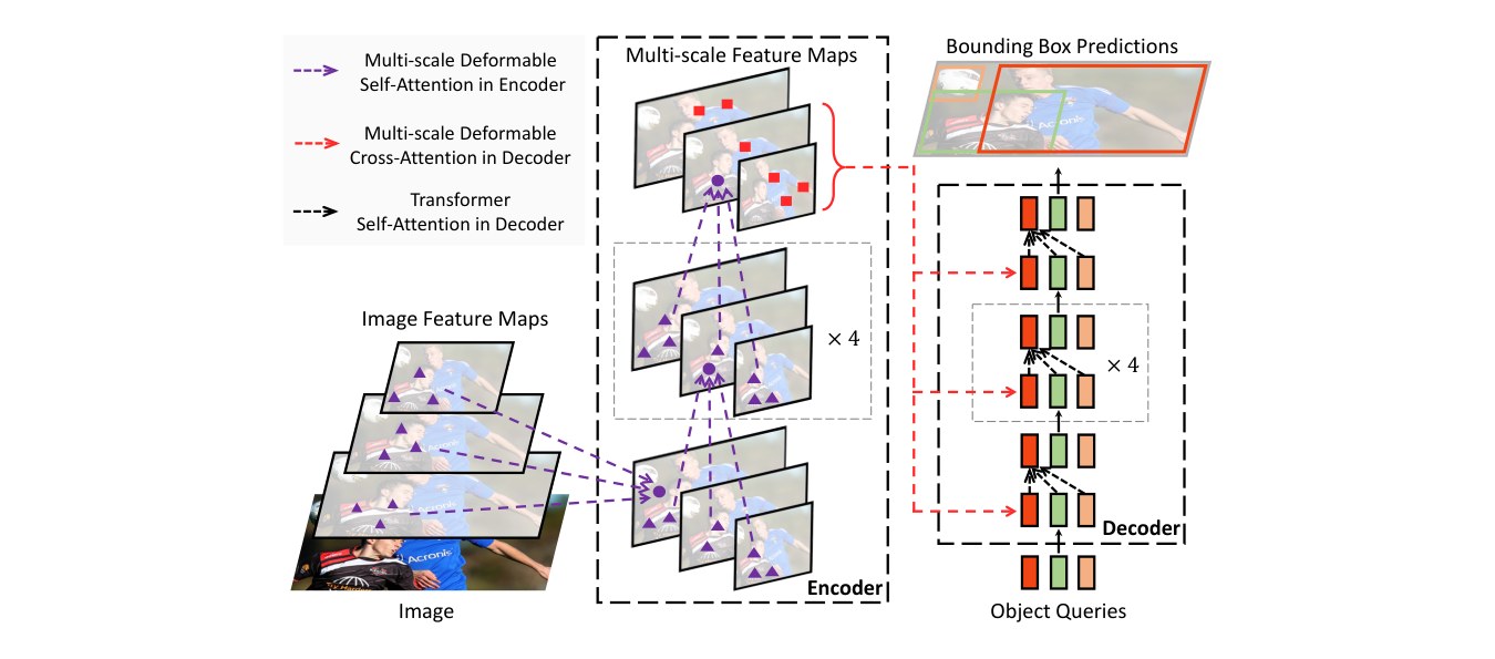
Figure 1: Illustration of the proposed Deformable DETR object detector.
图 1:所提 Deformable DETR 目标检测器示意。
2 Related Work
2 相关工作
Efficient Attention Mechanism. Transformers (Vaswani et al. 2017) involve both self-attention and cross-attention mechanisms. One of the most well-known concern of Transformers is the high time and memory complexity at vast key element numbers, which hinders model scalability in many cases. Recently, many efforts have been made to address this problem (Tay et al. 2020b), which can be roughly divided into three categories in practice.
高效注意力机制。 Transformer(Vaswani et al. 2017)同时包含自注意力与交叉注意力。广为人知的担忧之一是:当关键元素数量巨大时,时间与内存复杂度很高,许多情形下阻碍可扩展性。近期大量工作试图解决该问题(Tay et al. 2020b),实践中大致可分三类。
The first category is to use pre-defined sparse attention patterns on keys. The most straightforward paradigm is restricting the attention pattern to be fixed local windows. Most works (Liu et al. 2018a; Parmar et al. 2018; Child et al. 2019; Huang et al. 2019; Ho et al. 2019; Wang et al. 2020a; Hu et al. 2019; Ramachandran et al. 2019; Qiu et al. 2019; Beltagy et al. 2020; Ainslie et al. 2020; Zaheer et al. 2020) follow this paradigm. Although restricting the attention pattern to a local neighborhood can decrease the complexity, it loses global information. To compensate, Child et al. 2019; Huang et al. 2019; Ho et al. 2019; Wang et al. 2020a attend key elements at fixed intervals to significantly increase the receptive field on keys. Beltagy et al. 2020; Ainslie et al. 2020; Zaheer et al. 2020 allow a small number of special tokens having access to all key elements. Zaheer et al. 2020; Qiu et al. 2019 also add some pre-fixed sparse attention patterns to attend distant key elements directly.
第一类是对关键使用预定义稀疏注意力模式。最直接的范式是把注意力限制为固定局部窗口。多数工作(Liu et al. 2018a;Parmar et al. 2018;Child et al. 2019;Huang et al. 2019;Ho et al. 2019;Wang et al. 2020a;Hu et al. 2019;Ramachandran et al. 2019;Qiu et al. 2019;Beltagy et al. 2020;Ainslie et al. 2020;Zaheer et al. 2020)遵循这一范式。虽能降低复杂度,但会丢失全局信息。为补偿,Child et al. 2019;Huang et al. 2019;Ho et al. 2019;Wang et al. 2020a 以固定间隔关注关键元素,以显著扩大对关键的感受野。Beltagy et al. 2020;Ainslie et al. 2020;Zaheer et al. 2020 允许少数特殊 token 访问全部关键元素。Zaheer et al. 2020;Qiu et al. 2019 还加入若干预固定稀疏模式,以直接关注远处关键元素。
The second category is to learn data-dependent sparse attention. Kitaev et al. 2020 proposes a locality sensitive hashing (LSH) based attention, which hashes both the query and key elements to different bins. A similar idea is proposed by Roy et al. 2020, where k-means finds out the most related keys. Tay et al. 2020a learns block permutation for block-wise sparse attention.
第二类是学习数据依赖的稀疏注意力。Kitaev et al. 2020 提出基于局部敏感哈希(LSH)的注意力,把查询与关键元素哈希到不同桶。Roy et al. 2020 提出类似想法,用 k-means 找出最相关的键。Tay et al. 2020a 学习块置换以做块稀疏注意力。
The third category is to explore the low-rank property in self-attention. Wang et al. 2020b reduces the number of key elements through a linear projection on the size dimension instead of the channel dimension. Katharopoulos et al. 2020; Choromanski et al. 2020 rewrite the calculation of self-attention through kernelization approximation.
第三类探索自注意力中的低秩性质。Wang et al. 2020b 通过对尺寸维而非通道维做线性投影来减少关键元素数量。Katharopoulos et al. 2020;Choromanski et al. 2020 通过核化近似改写自注意力计算。
In the image domain, the designs of efficient attention mechanism (e.g., Parmar et al. 2018; Child et al. 2019; Huang et al. 2019; Ho et al. 2019; Wang et al. 2020a; Hu et al. 2019; Ramachandran et al. 2019) are still limited to the first category. Despite the theoretically reduced complexity, Ramachandran et al. 2019; Hu et al. 2019 admit such approaches are much slower in implementation than traditional convolution with the same FLOPs (at least 3 slower), due to the intrinsic limitation in memory access patterns.
在图像领域,高效注意力机制的设计(如 Parmar et al. 2018;Child et al. 2019;Huang et al. 2019;Ho et al. 2019;Wang et al. 2020a;Hu et al. 2019;Ramachandran et al. 2019)仍限于第一类。尽管理论复杂度下降,Ramachandran et al. 2019;Hu et al. 2019 承认:由于内存访问模式的固有限制,同等 FLOPs 下这类方法实现上仍比传统卷积慢得多(至少慢 3 倍)。
On the other hand, as discussed in Zhu et al. 2019a, there are variants of convolution, such as deformable convolution (Dai et al. 2017; Zhu et al. 2019b) and dynamic convolution (Wu et al. 2019), that also can be viewed as self-attention mechanisms. Especially, deformable convolution operates much more effectively and efficiently on image recognition than Transformer self-attention. Meanwhile, it lacks the element relation modeling mechanism.
另一方面,如 Zhu et al. 2019a 所讨论,也有可视为自注意力机制的卷积变体,例如可变形卷积(Dai et al. 2017;Zhu et al. 2019b)与动态卷积(Wu et al. 2019)。尤其是可变形卷积在图像识别上比 Transformer 自注意力更有效且高效;同时它缺少元素关系建模机制。
Our proposed deformable attention module is inspired by deformable convolution, and belongs to the second category. It only focuses on a small fixed set of sampling points predicted from the feature of query elements. Different from Ramachandran et al. 2019; Hu et al. 2019, deformable attention is just slightly slower than the traditional convolution under the same FLOPs.
我们提出的可变形注意力模块受可变形卷积启发,属于第二类。它只关注由查询元素特征预测的一小套固定采样点。与 Ramachandran et al. 2019;Hu et al. 2019 不同,同等 FLOPs 下可变形注意力仅略慢于传统卷积。
Multi-scale Feature Representation for Object Detection. One of the main difficulties in object detection is to effectively represent objects at vastly different scales. Modern object detectors usually exploit multi-scale features to accommodate this. As one of the pioneering works, FPN (Lin et al. 2017a) proposes a top-down path to combine multi-scale features. PANet (Liu et al. 2018b) further adds an bottom-up path on the top of FPN. Kong et al. 2018 combines features from all scales by a global attention operation. Zhao et al. 2019 proposes a U-shape module to fuse multi-scale features. Recently, NAS-FPN (Ghiasi et al. 2019) and Auto-FPN (Xu et al. 2019) are proposed to automatically design cross-scale connections via neural architecture search. Tan et al. 2020 proposes the BiFPN, which is a repeated simplified version of PANet. Our proposed multi-scale deformable attention module can naturally aggregate multi-scale feature maps via attention mechanism, without the help of these feature pyramid networks.
目标检测的多尺度特征表示。 目标检测的主要困难之一是有效表示尺度差异极大的物体。现代检测器通常利用多尺度特征应对。作为开创性工作之一,FPN(Lin et al. 2017a)提出自上而下路径以融合多尺度特征。PANet(Liu et al. 2018b)在 FPN 之上再加自下而上路径。Kong et al. 2018 用全局注意力操作融合所有尺度特征。Zhao et al. 2019 提出 U 形模块融合多尺度特征。近期 NAS-FPN(Ghiasi et al. 2019)与 Auto-FPN(Xu et al. 2019)通过神经架构搜索自动设计跨尺度连接。Tan et al. 2020 提出 BiFPN,即 PANet 的重复简化版。我们提出的多尺度可变形注意力模块可自然经由注意力机制聚合多尺度特征图,而无需这些特征金字塔网络。
3 Revisiting Transformers and DETR
3 回顾 Transformer 与 DETR
Multi-Head Attention in Transformers. Transformers (Vaswani et al. 2017) are of a network architecture based on attention mechanisms for machine translation. Given a query element (e.g., a target word in the output sentence) and a set of key elements (e.g., source words in the input sentence), the multi-head attention module adaptively aggregates the key contents according to the attention weights that measure the compatibility of query-key pairs. To allow the model focusing on contents from different representation subspaces and different positions, the outputs of different attention heads are linearly aggregated with learnable weights. Let indexes a query element with representation feature , and indexes a key element with representation feature , where is the feature dimension, and specify the set of query and key elements, respectively. Then the multi-head attention feature is calculated by
Transformer 中的多头注意力。 Transformer(Vaswani et al. 2017)是基于注意力机制的机器翻译网络结构。给定查询元素(例如输出句中的目标词)与一套关键元素(例如输入句中的源词),多头注意力模块 按衡量查询–关键对兼容性的注意力权重,自适应地聚合键内容。为使模型关注不同表示子空间与不同位置的内容,不同注意力头的输出用可学习权重线性聚合。令 索引具有表征特征 的查询元素, 索引具有表征特征 的关键元素,其中 为特征维, 与 分别指定查询与关键元素集合。则多头注意力特征计算为
where indexes the attention head, and are of learnable weights ( by default). The attention weights are normalized as , in which are also learnable weights. To disambiguate different spatial positions, the representation features and are usually of the concatenation/summation of element contents and positional embeddings.
其中 索引注意力头, 与 为可学习权重(默认 )。注意力权重 归一化为 ,其中 亦为可学习权重。为区分不同空间位置,表征特征 与 通常是元素内容与位置嵌入的拼接/求和。
There are two known issues with Transformers. One is Transformers need long training schedules before convergence. Suppose the number of query and key elements are of and , respectively. Typically, with proper parameter initialization, and follow distribution with mean of and variance of , which makes attention weights , when is large. It will lead to ambiguous gradients for input features. Thus, long training schedules are required so that the attention weights can focus on specific keys. In the image domain, where the key elements are usually of image pixels, can be very large and the convergence is tedious.
Transformer 有两个已知问题。其一是收敛前需要很长训练日程。设查询与关键元素数分别为 与 。通常在恰当参数初始化下, 与 服从均值 0、方差 1 的分布,当 很大时使注意力权重 ,从而给输入特征带来模糊梯度。因此需要很长训练,注意力权重才能聚焦特定键。在图像领域,关键元素通常是图像像素, 可以很大,收敛十分费力。
On the other hand, the computational and memory complexity for multi-head attention can be very high with numerous query and key elements. The computational complexity of Eq. 1 is of . In the image domain, where the query and key elements are both of pixels, , the complexity is dominated by the third term, as . Thus, the multi-head attention module suffers from a quadratic complexity growth with the feature map size.
另一方面,当查询与关键元素众多时,多头注意力的计算与内存复杂度可能很高。式 1 的计算复杂度为 。在图像领域,查询与关键都是像素,,复杂度由第三项主导,为 。因此多头注意力模块随特征图尺寸呈二次增长。
DETR. DETR (Carion et al. 2020) is built upon the Transformer encoder-decoder architecture, combined with a set-based Hungarian loss that forces unique predictions for each ground-truth bounding box via bipartite matching. We briefly review the network architecture as follows.
DETR。 DETR(Carion et al. 2020)建立在 Transformer 编码器–解码器结构之上,结合基于集合的 Hungarian 损失,通过二分匹配迫使每个真值边界框对应唯一预测。我们简要回顾网络结构如下。
Given the input feature maps extracted by a CNN backbone (e.g., ResNet (He et al. 2016)), DETR exploits a standard Transformer encoder-decoder architecture to transform the input feature maps to be features of a set of object queries. A 3-layer feed-forward neural network (FFN) and a linear projection are added on top of the object query features (produced by the decoder) as the detection head. The FFN acts as the regression branch to predict the bounding box coordinates , where encodes the normalized box center coordinates, box height and width (relative to the image size). The linear projection acts as the classification branch to produce the classification results.
给定 CNN 骨干(如 ResNet,He et al. 2016)提取的输入特征图 ,DETR 用标准 Transformer 编码器–解码器把输入特征图变换为一套物体查询的特征。在解码器产出的物体查询特征之上,再接 3 层前馈网络(FFN)与线性投影作为检测头。FFN 作为回归分支,预测边界框坐标 ,其中 编码相对图像尺寸归一化的框中心坐标、高度与宽度。线性投影作为分类分支,产生分类结果。
For the Transformer encoder in DETR, both query and key elements are of pixels in the feature maps. The inputs are of ResNet feature maps (with encoded positional embeddings). Let and denote the feature map height and width, respectively. The computational complexity of self-attention is of , which grows quadratically with the spatial size.
对 DETR 中的 Transformer 编码器,查询与关键元素都是特征图中的像素。输入为(编码了位置嵌入的)ResNet 特征图。令 与 分别表示特征图高与宽,自注意力计算复杂度为 ,随空间尺寸二次增长。
For the Transformer decoder in DETR, the input includes both feature maps from the encoder, and object queries represented by learnable positional embeddings (e.g., ). There are two types of attention modules in the decoder, namely, cross-attention and self-attention modules. In the cross-attention modules, object queries extract features from the feature maps. The query elements are of the object queries, and key elements are of the output feature maps from the encoder. In it, , and the complexity of the cross-attention is of . The complexity grows linearly with the spatial size of feature maps. In the self-attention modules, object queries interact with each other, so as to capture their relations. The query and key elements are both of the object queries. In it, , and the complexity of the self-attention module is of . The complexity is acceptable with moderate number of object queries.
对 DETR 中的 Transformer 解码器,输入包括来自编码器的特征图,以及由可学习位置嵌入表示的 个物体查询(例如 )。解码器中有两类注意力模块:交叉注意力与自注意力。在交叉注意力中,物体查询从特征图提取特征:查询元素是物体查询,关键元素是编码器输出特征图。此时 ,,交叉注意力复杂度为 ,随特征图空间尺寸线性增长。在自注意力中,物体查询彼此交互以捕获关系:查询与关键都是物体查询。此时 ,自注意力复杂度为 ;在物体查询数量适中时该复杂度可接受。
DETR is an attractive design for object detection, which removes the need for many hand-designed components. However, it also has its own issues. These issues can be mainly attributed to the deficits of Transformer attention in handling image feature maps as key elements: (1) DETR has relatively low performance in detecting small objects. Modern object detectors use high-resolution feature maps to better detect small objects. However, high-resolution feature maps would lead to an unacceptable complexity for the self-attention module in the Transformer encoder of DETR, which has a quadratic complexity with the spatial size of input feature maps. (2) Compared with modern object detectors, DETR requires many more training epochs to converge. This is mainly because the attention modules processing image features are difficult to train. For example, at initialization, the cross-attention modules are almost of average attention on the whole feature maps. While, at the end of the training, the attention maps are learned to be very sparse, focusing only on the object extremities. It seems that DETR requires a long training schedule to learn such significant changes in the attention maps.
DETR 是有吸引力的目标检测设计,去掉了许多手工组件。但它也有自身问题,主要可归因于 Transformer 注意力在把图像特征图作为关键元素时的不足:(1)DETR 检测小物体相对偏弱。现代检测器用高分辨率特征图更好检测小物体;但高分辨率特征图会使 DETR Transformer 编码器中随输入特征图空间尺寸二次增长的自注意力复杂度变得不可接受。(2)相较现代检测器,DETR 需要多得多的训练轮数才能收敛。这主要因为处理图像特征的注意力模块难以训练。例如初始化时,交叉注意力模块几乎对整张特征图平均关注;而训练结束时,注意力图已学得很稀疏,只聚焦物体边缘。似乎 DETR 需要很长训练日程,才能学会注意力图上如此显著的变化。
4 Method
4 方法
4.1 Deformable Transformers for End-to-End Object Detection
4.1 面向端到端目标检测的可变形 Transformer
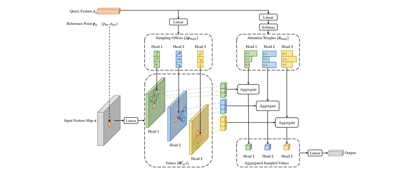
Figure 2: Illustration of the proposed deformable attention module.
图 2:所提可变形注意力模块示意。
Deformable Attention Module. The core issue of applying Transformer attention on image feature maps is that it would look over all possible spatial locations. To address this, we present a deformable attention module. Inspired by deformable convolution (Dai et al. 2017; Zhu et al. 2019b), the deformable attention module only attends to a small set of key sampling points around a reference point, regardless of the spatial size of the feature maps, as shown in Fig. 2. By assigning only a small fixed number of keys for each query, the issues of convergence and feature spatial resolution can be mitigated.
可变形注意力模块。 把 Transformer 注意力用在图像特征图上的核心问题是:它会扫过所有可能的空间位置。为此我们提出 可变形注意力模块。受可变形卷积(Dai et al. 2017;Zhu et al. 2019b)启发,该模块只关注参考点周围一小套关键采样点,而与特征图空间尺寸无关,如图 2 所示。通过为每个查询只分配固定少量键,收敛与特征空间分辨率问题可得到缓解。
Given an input feature map , let index a query element with content feature and a 2-d reference point , the deformable attention feature is calculated by
给定输入特征图 ,令 索引具有内容特征 与二维参考点 的查询元素,可变形注意力特征计算为
where indexes the attention head, indexes the sampled keys, and is the total sampled key number (). and denote the sampling offset and attention weight of the sampling point in the attention head, respectively. The scalar attention weight lies in the range , normalized by . are of 2-d real numbers with unconstrained range. As is fractional, bilinear interpolation is applied as in Dai et al. 2017 in computing . Both and are obtained via linear projection over the query feature . In implementation, the query feature is fed to a linear projection operator of channels, where the first channels encode the sampling offsets , and the remaining channels are fed to a operator to obtain the attention weights .
其中 索引注意力头, 索引采样键, 为采样键总数()。 与 分别表示第 个注意力头中第 个采样点的采样偏移与注意力权重。标量注意力权重 落在 ,并由 归一化。 为范围无约束的二维实数。由于 可为分数,计算 时按 Dai et al. 2017 使用双线性插值。 与 均由查询特征 经线性投影得到。实现上,将 送入通道数为 的线性投影:前 通道编码采样偏移 ,其余 通道经 得到注意力权重 。
The deformable attention module is designed for processing convolutional feature maps as key elements. Let be the number of query elements, when is relatively small, the complexity of the deformable attention module is of (See Appendix A.1 for details). When it is applied in DETR encoder, where , the complexity becomes , which is of linear complexity with the spatial size. When it is applied as the cross-attention modules in DETR decoder, where ( is the number of object queries), the complexity becomes , which is irrelevant to the spatial size .
可变形注意力模块专为把卷积特征图作为关键元素而设计。令 为查询元素数,当 相对较小时,模块复杂度为 (细节见附录 A.1)。用于 DETR 编码器且 时,复杂度变为 ,随空间尺寸线性增长;用作 DETR 解码器交叉注意力且 ( 为物体查询数)时,复杂度变为 ,与空间尺寸 无关。
Multi-scale Deformable Attention Module. Most modern object detection frameworks benefit from multi-scale feature maps (Liu et al. 2020). Our proposed deformable attention module can be naturally extended for multi-scale feature maps.
多尺度可变形注意力模块。 多数现代目标检测框架受益于多尺度特征图(Liu et al. 2020)。所提可变形注意力模块可自然扩展到多尺度特征图。
Let be the input multi-scale feature maps, where . Let be the normalized coordinates of the reference point for each query element , then the multi-scale deformable attention module is applied as
令 为输入多尺度特征图,其中 。令 为每个查询元素 的参考点归一化坐标,则多尺度可变形注意力模块作用为
where indexes the attention head, indexes the input feature level, and indexes the sampling point. and denote the sampling offset and attention weight of the sampling point in the feature level and the attention head, respectively. The scalar attention weight is normalized by . Here, we use normalized coordinates for the clarity of scale formulation, in which the normalized coordinates and indicate the top-left and the bottom-right image corners, respectively. Function in Equation 3 re-scales the normalized coordinates to the input feature map of the -th level. The multi-scale deformable attention is very similar to the previous single-scale version, except that it samples points from multi-scale feature maps instead of points from single-scale feature maps.
其中 索引注意力头, 索引输入特征层级, 索引采样点。 与 分别表示第 特征层、第 注意力头中第 个采样点的采样偏移与注意力权重。标量注意力权重 由 归一化。此处用归一化坐标 以便清晰表述尺度: 与 分别对应图像左上与右下角。式 3 中函数 把归一化坐标 重新缩放到第 层输入特征图。多尺度可变形注意力与前述单尺度版本十分相似,只是从多尺度特征图采样 个点,而非从单尺度采样 个点。
The proposed attention module will degenerate to deformable convolution (Dai et al. 2017), when , , and is fixed as an identity matrix. Deformable convolution is designed for single-scale inputs, focusing only on one sampling point for each attention head. However, our multi-scale deformable attention looks over multiple sampling points from multi-scale inputs. The proposed (multi-scale) deformable attention module can also be perceived as an efficient variant of Transformer attention, where a pre-filtering mechanism is introduced by the deformable sampling locations. When the sampling points traverse all possible locations, the proposed attention module is equivalent to Transformer attention.
当 、,且 固定为单位矩阵时,所提注意力模块退化为可变形卷积(Dai et al. 2017)。可变形卷积面向单尺度输入,每个注意力头只关注一个采样点;而我们的多尺度可变形注意力从多尺度输入查看多个采样点。所提(多尺度)可变形注意力也可视为 Transformer 注意力的高效变体:由可变形采样位置引入预过滤机制。当采样点遍历全部可能位置时,所提注意力模块等价于 Transformer 注意力。
Deformable Transformer Encoder. We replace the Transformer attention modules processing feature maps in DETR with the proposed multi-scale deformable attention module. Both the input and output of the encoder are of multi-scale feature maps with the same resolutions. In encoder, we extract multi-scale feature maps () from the output feature maps of stages through in ResNet (He et al. 2016) (transformed by a convolution), where is of resolution lower than the input image. The lowest resolution feature map is obtained via a stride convolution on the final stage, denoted as . All the multi-scale feature maps are of channels. Note that the top-down structure in FPN (Lin et al. 2017a) is not used, because our proposed multi-scale deformable attention in itself can exchange information among multi-scale feature maps. The constructing of multi-scale feature maps are also illustrated in Appendix A.2. Experiments in Section 5.2 show that adding FPN will not improve the performance.
可变形 Transformer 编码器。 我们用所提多尺度可变形注意力模块替换 DETR 中处理特征图的 Transformer 注意力模块。编码器输入与输出均为相同分辨率的多尺度特征图。编码器中,我们从 ResNet(He et al. 2016)阶段 到 的输出特征图(经 卷积变换)提取多尺度特征图 (),其中 分辨率比输入图像低 倍。最低分辨率特征图 由最终 阶段上 、步长 2 的卷积得到,记为 。全部多尺度特征图通道数为 。注意未使用 FPN(Lin et al. 2017a)中的自上而下结构,因为所提多尺度可变形注意力本身即可在多尺度特征图之间交换信息。多尺度特征图的构建亦见附录 A.2。第 5.2 节实验表明加入 FPN 不会提升表现。
In application of the multi-scale deformable attention module in encoder, the output are of multi-scale feature maps with the same resolutions as the input. Both the key and query elements are of pixels from the multi-scale feature maps. For each query pixel, the reference point is itself. To identify which feature level each query pixel lies in, we add a scale-level embedding, denoted as , to the feature representation, in addition to the positional embedding. Different from the positional embedding with fixed encodings, the scale-level embedding are randomly initialized and jointly trained with the network.
在编码器中应用多尺度可变形注意力时,输出为与输入同分辨率的多尺度特征图。键与查询元素都是多尺度特征图中的像素。对每个查询像素,参考点即其自身。为标识查询像素所处特征层级,除位置嵌入外,我们再加入尺度层级嵌入 。与固定编码的位置嵌入不同,尺度层级嵌入 随机初始化并与网络联合训练。
Deformable Transformer Decoder. There are cross-attention and self-attention modules in the decoder. The query elements for both types of attention modules are of object queries. In the cross-attention modules, object queries extract features from the feature maps, where the key elements are of the output feature maps from the encoder. In the self-attention modules, object queries interact with each other, where the key elements are of the object queries. Since our proposed deformable attention module is designed for processing convolutional feature maps as key elements, we only replace each cross-attention module to be the multi-scale deformable attention module, while leaving the self-attention modules unchanged. For each object query, the 2-d normalized coordinate of the reference point is predicted from its object query embedding via a learnable linear projection followed by a function.
可变形 Transformer 解码器。 解码器中有交叉注意力与自注意力模块。两类注意力的查询元素都是物体查询。在交叉注意力中,物体查询从特征图提取特征,关键元素是编码器输出特征图;在自注意力中,物体查询彼此交互,关键元素是物体查询。由于所提可变形注意力专为把卷积特征图作为关键而设计,我们只把每个交叉注意力替换为多尺度可变形注意力,而保持自注意力不变。对每个物体查询,参考点的二维归一化坐标 由其物体查询嵌入经可学习线性投影再接 预测得到。
Because the multi-scale deformable attention module extracts image features around the reference point, we let the detection head predict the bounding box as relative offsets w.r.t. the reference point to further reduce the optimization difficulty. The reference point is used as the initial guess of the box center. The detection head predicts the relative offsets w.r.t. the reference point. Check Appendix A.3 for the details. In this way, the learned decoder attention will have strong correlation with the predicted bounding boxes, which also accelerates the training convergence.
由于多尺度可变形注意力在参考点周围提取图像特征,我们让检测头把边界框预测为相对参考点的偏移,以进一步降低优化难度。参考点用作框中心的初始猜测,检测头预测相对该参考点的偏移。细节见附录 A.3。如此,学到的解码器注意力将与预测边界框强相关,也加速训练收敛。
By replacing Transformer attention modules with deformable attention modules in DETR, we establish an efficient and fast converging detection system, dubbed as Deformable DETR (see Fig. 1).
用可变形注意力模块替换 DETR 中的 Transformer 注意力后,我们得到高效且快速收敛的检测系统,称为 Deformable DETR(见图 1)。
4.2 Additional Improvements and Variants for Deformable DETR
4.2 Deformable DETR 的额外改进与变体
Deformable DETR opens up possibilities for us to exploit various variants of end-to-end object de-tectors, thanks to its fast convergence, and computational and memory efficiency. Due to limited space, we only introduce the core ideas of these improvements and variants here. The implementation details are given in Appendix A.4.
得益于快速收敛以及计算与内存效率,Deformable DETR 使我们有机会探索端到端目标检测器的多种变体。
Iterative Bounding Box Refinement. This is inspired by the iterative refinement developed in optical flow estimation (Teed & Deng 2020). We establish a simple and effective iterative bounding box refinement mechanism to improve detection performance. Here, each decoder layer refines the bounding boxes based on the predictions from the previous layer.
迭代边界框精炼。 灵感来自光流估计中的迭代精炼(Sun et al. 2018;Teed and Deng 2020)。这里每个解码器层精炼前一层给出的边界框预测。具体地,第 层解码器把相对前一层框坐标的偏移作为预测,细节见附录 A.4。
Two-Stage Deformable DETR. In the original DETR, object queries in the decoder are irrelevant to the current image. Inspired by two-stage object detectors, we explore a variant of Deformable DETR for generating region proposals as the first stage. The generated region proposals will be fed into the decoder as object queries for further refinement, forming a two-stage Deformable DETR.
两阶段 Deformable DETR。 在原始 DETR 中,解码器的物体查询是与图像内容无关的可学习参数。我们探索生成区域提议作为物体查询的两阶段结构:第一阶段生成区域提议,第二阶段把它们作为物体查询送入解码器做精炼。
In the first stage, to achieve high-recall proposals, each pixel in the multi-scale feature maps would serve as an object query. However, directly setting object queries as pixels will bring unacceptable computational and memory cost for the self-attention modules in the decoder, whose complexity grows quadratically with the number of queries. To avoid this problem, we remove the decoder and form an encoder-only Deformable DETR for region proposal generation. In it, each pixel is assigned as an object query, which directly predicts a bounding box. Top scoring bounding boxes are picked as region proposals. No NMS is applied before feeding the region proposals to the second stage.
在第一阶段,为获得高召回提议,多尺度特征图中每个像素都被视为物体查询,用多尺度可变形注意力做自注意力以增强特征,再由检测头预测边界框与二分类分数(前景对背景)。取分数最高的边界框作为区域提议。在第二阶段,这些区域提议作为物体查询送入解码器,做迭代边界框精炼。细节见附录 A.4。注意第一阶段也是 Deformable DETR 的变体,只是物体查询是密集的像素。
5 Experiment
5 实验
Dataset. We conduct experiments on COCO 2017 dataset (Lin et al. 2014). Our models are trained on the train set, and evaluated on the val set and test-dev set.
数据集。 我们在 COCO 2017 数据集(Lin et al. 2014)上实验。模型在 train 集上训练,在 val 集上评估。
Implementation Details. ImageNet (Deng et al. 2009) pre-trained ResNet-50 (He et al. 2016) is utilized as the backbone for ablations. Multi-scale feature maps are extracted without FPN (Lin et al. 2017a). and are set for deformable attentions by default. Parameters of the deformable Transformer encoder are shared among different feature levels. Other hyper-parameter setting and training strategy mainly follow DETR (Carion et al. 2020), except that Focal Loss (Lin et al. 2017b) with loss weight of 2 is used for bounding box classification, and the number of object queries is increased from 100 to 300. We also report the performance of DETR-DC5 with these modifications for a fair comparison, denoted as DETR-DC5+. By default, models are trained for 50 epochs and the learning rate is decayed at the 40-th epoch by a factor of 0.1. Following DETR(Carion et al. 2020), we train our models using Adam optimizer (Kingma & Ba 2015) with base learning rate of , , , and weight decay of . Learning rates of the linear projections, used for predicting object query reference points and sampling offsets, are multiplied by a factor of 0.1. Run time is evaluated on NVIDIA Tesla V100 GPU.
实现细节。 消融实验以 ImageNet(Deng et al. 2009)预训练的 ResNet-50(He et al. 2016)为骨干。多尺度特征图在不使用 FPN(Lin et al. 2017a)的情况下提取。可变形注意力默认 、。可变形 Transformer 编码器参数在不同特征层间共享。其余超参与训练策略主要沿袭 DETR(Carion et al. 2020),但边界框分类使用损失权重为 2 的 Focal Loss(Lin et al. 2017b),并把物体查询数从 100 增至 300。为公平比较,我们也报告带这些改动的 DETR-DC5 表现,记为 DETR-DC5+。默认训练 50 轮,学习率在第 40 轮按 0.1 倍衰减。沿袭 DETR(Carion et al. 2020),用 Adam 优化器(Kingma & Ba 2015),基础学习率 ,,,权重衰减 。用于预测物体查询参考点与采样偏移的线性投影,学习率再乘 0.1。运行时间在 NVIDIA Tesla V100 GPU 上评估。
5.1 Comparison with DETR
5.1 与 DETR 比较
As shown in Table 1, compared with Faster R-CNN + FPN, DETR requires many more training epochs to converge, and delivers lower performance at detecting small objects. Compared with DETR, Deformable DETR achieves better performance (especially on small objects) with 10 less training epochs. Detailed convergence curves are shown in Fig. 3. With the aid of iterative bounding box refinement and two-stage paradigm, our method can further improve the detection accuracy.
如表 1 所示,相较 Faster R-CNN + FPN,DETR 需要多得多的训练轮数才能收敛,且在小物体上表现较差。DETR-DC5 用扩张 C5 特征以增大特征分辨率,改善小物体检测,但显著增加 FLOPs 与 GPU 内存。
Our proposed Deformable DETR has on par FLOPs with Faster R-CNN + FPN and DETR-DC5. But the runtime speed is much faster (1.6) than DETR-DC5, and is just 25% slower than Faster R-CNN + FPN. The speed issue of DETR-DC5 is mainly due to the large amount of memory access in Transformer attention. Our proposed deformable attention can mitigate this issue, at the cost of unordered memory access. Thus, it is still slightly slower than traditional convolution.
所提 Deformable DETR 的 FLOPs 与 Faster R-CNN + FPN 及 DETR-DC5 相当,而参数更少。它以 50 轮训练即显著优于训练 500 轮的 DETR,尤其在小物体上。如图 3 所示,Deformable DETR 收敛远快于 DETR。
| Method | Epochs | AP | AP | AP | AP | AP | AP | params | FLOPs | Training GPU hours | Training | GPU hours | Inference FPS | Inference | FPS |
|---|---|---|---|---|---|---|---|---|---|---|---|---|---|---|---|
| Training | |||||||||||||||
| GPU hours | |||||||||||||||
| Inference | |||||||||||||||
| FPS | |||||||||||||||
| Faster R-CNN + FPN | 109 | 42.0 | 62.1 | 45.5 | 26.6 | 45.4 | 53.4 | 42M | 180G | 380 | 26 | ||||
| DETR | 500 | 42.0 | 62.4 | 44.2 | 20.5 | 45.8 | 61.1 | 41M | 86G | 2000 | 28 | ||||
| DETR-DC5 | 500 | 43.3 | 63.1 | 45.9 | 22.5 | 47.3 | 61.1 | 41M | 187G | 7000 | 12 | ||||
| DETR-DC5 | 50 | 35.3 | 55.7 | 36.8 | 15.2 | 37.5 | 53.6 | 41M | 187G | 700 | 12 | ||||
| DETR-DC5+ | 50 | 36.2 | 57.0 | 37.4 | 16.3 | 39.2 | 53.9 | 41M | 187G | 700 | 12 | ||||
| Deformable DETR | 50 | 43.8 | 62.6 | 47.7 | 26.4 | 47.1 | 58.0 | 40M | 173G | 325 | 19 | ||||
| + iterative bounding box refinement | 50 | 45.4 | 64.7 | 49.0 | 26.8 | 48.3 | 61.7 | 40M | 173G | 325 | 19 | ||||
| ++ two-stage Deformable DETR | 50 | 46.2 | 65.2 | 50.0 | 28.8 | 49.2 | 61.7 | 40M | 173G | 340 | 19 |
| Training |
|---|
| GPU hours |
| Inference |
|---|
| FPS |
Table 1: Comparision of Deformable DETR with DETR on COCO 2017 val set. DETR-DC5+ denotes DETR-DC5 with Focal Loss and 300 object queries.
| 方法 | 轮数 | AP | AP | AP | AP | AP | AP | 参数 | FLOPs | 训练 GPU 小时 | 推理 FPS |
|---|---|---|---|---|---|---|---|---|---|---|---|
| Faster R-CNN + FPN | 109 | 42.0 | 62.1 | 45.5 | 26.6 | 45.4 | 53.4 | 42M | 180G | 380 | 26 |
| DETR | 500 | 42.0 | 62.4 | 44.2 | 20.5 | 45.8 | 61.1 | 41M | 86G | 2000 | 28 |
| DETR-DC5 | 500 | 43.3 | 63.1 | 45.9 | 22.5 | 47.3 | 61.1 | 41M | 187G | 7000 | 12 |
| DETR-DC5 | 50 | 35.3 | 55.7 | 36.8 | 15.2 | 37.5 | 53.6 | 41M | 187G | 700 | 12 |
| DETR-DC5+ | 50 | 36.2 | 57.0 | 37.4 | 16.3 | 39.2 | 53.9 | 41M | 187G | 700 | 12 |
| Deformable DETR | 50 | 43.8 | 62.6 | 47.7 | 26.4 | 47.1 | 58.0 | 40M | 173G | 325 | 19 |
| + 迭代边界框精炼 | 50 | 45.4 | 64.7 | 49.0 | 26.8 | 48.3 | 61.7 | 40M | 173G | 325 | 19 |
| ++ 两阶段 Deformable DETR | 50 | 46.2 | 65.2 | 50.0 | 28.8 | 49.2 | 61.7 | 40M | 173G | 340 | 19 |
表 1:在 COCO 2017 val 集上 Deformable DETR 与 DETR 的比较。DETR-DC5+ 表示带 Focal Loss 且物体查询数为 300 的 DETR-DC5。
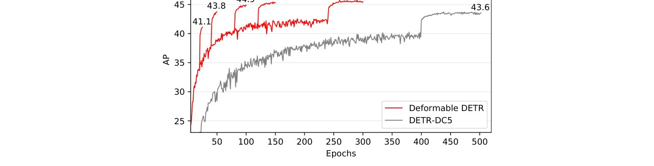
Figure 3: Convergence curves of Deformable DETR and DETR-DC5 on COCO 2017 val set. For Deformable DETR, we explore different training schedules by varying the epochs at which the learning rate is reduced (where the AP score leaps).
图 3:Deformable DETR 与 DETR-DC5 在 COCO 2017 val 集上的收敛曲线。对 Deformable DETR,我们探索不同训练轮数。
5.2 Ablation Study on Deformable Attention
5.2 可变形注意力消融
Table 2 presents ablations for various design choices of the proposed deformable attention module. Using multi-scale inputs instead of single-scale inputs can effectively improve detection accuracy with AP, especially on small objects with AP. Increasing the number of sampling points can further improve AP. Using multi-scale deformable attention, which allows information exchange among different scale levels, can bring additional improvement in AP. Because the cross-level feature exchange is already adopted, adding FPNs will not improve the performance. When multi-scale attention is not applied, and , our (multi-scale) deformable attention module degenerates to deformable convolution, delivering noticeable lower accuracy.
表 2 给出所提可变形注意力多种设计选择的消融。多尺度输入与多尺度注意力都对良好表现至关重要。增大每查询采样点数 可提升表现,但收益在 后趋于饱和。加入 FPN 不会带来额外提升,说明多尺度可变形注意力已能有效交换多尺度信息。
| MS inputs | MS attention | K | FPNs | AP | AP | AP | AP | AP | AP |
|---|---|---|---|---|---|---|---|---|---|
| 4 | FPN (Lin et al. 2017a) | 43.8 | 62.6 | 47.8 | 26.5 | 47.3 | 58.1 | ||
| 4 | BiFPN (Tan et al. 2020) | 43.9 | 62.5 | 47.7 | 25.6 | 47.4 | 57.7 | ||
| 1 | w/o | 39.7 | 60.1 | 42.4 | 21.2 | 44.3 | 56.0 | ||
| 1 | 41.4 | 60.9 | 44.9 | 24.1 | 44.6 | 56.1 | |||
| 4 | 42.3 | 61.4 | 46.0 | 24.8 | 45.1 | 56.3 | |||
| 4 | 43.8 | 62.6 | 47.7 | 26.4 | 47.1 | 58.0 |
Table 2: Ablations for deformable attention on COCO 2017 val set. “MS inputs” indicates using multi-scale inputs. “MS attention” indicates using multi-scale deformable attention. is the number of sampling points for each attention head on each feature level.
| 多尺度输入 | 多尺度注意力 | K | FPN | AP | AP | AP | AP | AP | AP |
|---|---|---|---|---|---|---|---|---|---|
| 4 | FPN(Lin et al. 2017a) | 43.8 | 62.6 | 47.8 | 26.5 | 47.3 | 58.1 | ||
| 4 | BiFPN(Tan et al. 2020) | 43.9 | 62.5 | 47.7 | 25.6 | 47.4 | 57.7 | ||
| 1 | 无 | 39.7 | 60.1 | 42.4 | 21.2 | 44.3 | 56.0 | ||
| 1 | 41.4 | 60.9 | 44.9 | 24.1 | 44.6 | 56.1 | |||
| 4 | 42.3 | 61.4 | 46.0 | 24.8 | 45.1 | 56.3 | |||
| 4 | 43.8 | 62.6 | 47.7 | 26.4 | 47.1 | 58.0 |
表 2:在 COCO 2017 val 集上对可变形注意力的消融。「多尺度输入」表示使用多尺度输入。「多尺度注意力」表示使用多尺度可变形注意力。 为每个注意力头在每个特征层上的采样点数。
5.3 Comparison with State-of-the-art Methods
5.3 与先进方法比较
Table 3 compares the proposed method with other state-of-the-art methods. Iterative bounding box refinement and two-stage mechanism are both utilized by our models in Table 3. With ResNet-101 and ResNeXt-101 (Xie et al. 2017), our method achieves 48.7 AP and 49.0 AP without bells and whistles, respectively. By using ResNeXt-101 with DCN (Zhu et al. 2019b), the accuracy rises to 50.1 AP. With additional test-time augmentations, the proposed method achieves 52.3 AP.
表 3 将所提方法与其他先进方法比较。表 3 中我们的模型同时使用迭代边界框精炼与两阶段机制。使用 ResNet-101 与 ResNeXt-101(Xie et al. 2017)时,方法在无额外技巧下分别达到 48.7 AP 与 49.0 AP。使用带 DCN(Zhu et al. 2019b)的 ResNeXt-101 时,精度升至 50.1 AP。再加测试时增强,所提方法达到 52.3 AP。
| Method | Backbone | TTA | AP | AP | AP | AP | AP | AP |
|---|---|---|---|---|---|---|---|---|
| FCOS (Tian et al. 2019) | ResNeXt-101 | 44.7 | 64.1 | 48.4 | 27.6 | 47.5 | 55.6 | |
| ATSS (Zhang et al. 2020) | ResNeXt-101 + DCN | 50.7 | 68.9 | 56.3 | 33.2 | 52.9 | 62.4 | |
| TSD (Song et al. 2020) | SENet154 + DCN | 51.2 | 71.9 | 56.0 | 33.8 | 54.8 | 64.2 | |
| EfficientDet-D7 (Tan et al. 2020) | EfficientNet-B6 | 52.2 | 71.4 | 56.3 | - | - | - | |
| Deformable DETR | ResNet-50 | 46.9 | 66.4 | 50.8 | 27.7 | 49.7 | 59.9 | |
| Deformable DETR | ResNet-101 | 48.7 | 68.1 | 52.9 | 29.1 | 51.5 | 62.0 | |
| Deformable DETR | ResNeXt-101 | 49.0 | 68.5 | 53.2 | 29.7 | 51.7 | 62.8 | |
| Deformable DETR | ResNeXt-101 + DCN | 50.1 | 69.7 | 54.6 | 30.6 | 52.8 | 64.7 | |
| Deformable DETR | ResNeXt-101 + DCN | 52.3 | 71.9 | 58.1 | 34.4 | 54.4 | 65.6 |
Table 3: Comparison of Deformable DETR with state-of-the-art methods on COCO 2017 test-dev set. “TTA” indicates test-time augmentations including horizontal flip and multi-scale testing.
| 方法 | 骨干 | TTA | AP | AP | AP | AP | AP | AP |
|---|---|---|---|---|---|---|---|---|
| FCOS(Tian et al. 2019) | ResNeXt-101 | 44.7 | 64.1 | 48.4 | 27.6 | 47.5 | 55.6 | |
| ATSS(Zhang et al. 2020) | ResNeXt-101 + DCN | 50.7 | 68.9 | 56.3 | 33.2 | 52.9 | 62.4 | |
| TSD(Song et al. 2020) | SENet154 + DCN | 51.2 | 71.9 | 56.0 | 33.8 | 54.8 | 64.2 | |
| EfficientDet-D7(Tan et al. 2020) | EfficientNet-B6 | 52.2 | 71.4 | 56.3 | - | - | - | |
| Deformable DETR | ResNet-50 | 46.9 | 66.4 | 50.8 | 27.7 | 49.7 | 59.9 | |
| Deformable DETR | ResNet-101 | 48.7 | 68.1 | 52.9 | 29.1 | 51.5 | 62.0 | |
| Deformable DETR | ResNeXt-101 | 49.0 | 68.5 | 53.2 | 29.7 | 51.7 | 62.8 | |
| Deformable DETR | ResNeXt-101 + DCN | 50.1 | 69.7 | 54.6 | 30.6 | 52.8 | 64.7 | |
| Deformable DETR | ResNeXt-101 + DCN | 52.3 | 71.9 | 58.1 | 34.4 | 54.4 | 65.6 |
表 3:在 COCO 2017 test-dev 上 Deformable DETR 与先进方法比较。「TTA」表示含水平翻转与多尺度测试的测试时增强。
6 Conclusion
6 结论
Deformable DETR is an end-to-end object detector, which is efficient and fast-converging. It enables us to explore more interesting and practical variants of end-to-end object detectors. At the core of Deformable DETR are the (multi-scale) deformable attention modules, which is an efficient attention mechanism in processing image feature maps. We hope our work opens up new possibilities in exploring end-to-end object detection.
Deformable DETR 是高效且快速收敛的端到端目标检测器。它使我们能够探索更有趣且实用的端到端检测器变体。其核心是(多尺度)可变形注意力模块——一种处理图像特征图的高效注意力机制。我们希望本工作为探索端到端目标检测打开新的可能。
Acknowledgments
The work is supported by the National Key R&D Program of China (2020AAA0105200), Beijing Academy of Artificial Intelligence, and the National Natural Science Foundation of China under grand No.U19B2044 and No.61836011.
致谢
本工作得到国家重点研发计划(2020AAA0105200)、北京智源人工智能研究院,以及国家自然科学基金(批准号 U19B2044 与 61836011)支持。
References
参考文献
Ainslie et al. (2020) Joshua Ainslie, Santiago Ontanon, Chris Alberti, Philip Pham, Anirudh Ravula, and Sumit Sanghai. Etc: Encoding long and structured data in transformers. arXiv preprint arXiv:2004.08483 , 2020.
Beltagy et al. (2020) Iz Beltagy, Matthew E Peters, and Arman Cohan. Longformer: The long-document transformer. arXiv preprint arXiv:2004.05150 , 2020.
Carion et al. (2020) Nicolas Carion, Francisco Massa, Gabriel Synnaeve, Nicolas Usunier, Alexander Kirillov, and Sergey Zagoruyko. End-to-end object detection with transformers. In ECCV , 2020.
Child et al. (2019) Rewon Child, Scott Gray, Alec Radford, and Ilya Sutskever. Generating long sequences with sparse transformers. arXiv preprint arXiv:1904.10509 , 2019.
Choromanski et al. (2020) Krzysztof Choromanski, Valerii Likhosherstov, David Dohan, Xingyou Song, Jared Davis, Tamas Sarlos, David Belanger, Lucy Colwell, and Adrian Weller. Masked language modeling for proteins via linearly scalable long-context transformers. arXiv preprint arXiv:2006.03555 , 2020.
Dai et al. (2017) Jifeng Dai, Haozhi Qi, Yuwen Xiong, Yi Li, Guodong Zhang, Han Hu, and Yichen Wei. Deformable convolutional networks. In ICCV , 2017.
Deng et al. (2009) Jia Deng, Wei Dong, Richard Socher, Li-Jia Li, Kai Li, and Li Fei-Fei. Imagenet: A large-scale hierarchical image database. In CVPR , 2009.
Ghiasi et al. (2019) Golnaz Ghiasi, Tsung-Yi Lin, and Quoc V Le. Nas-fpn: Learning scalable feature pyramid architecture for object detection. In CVPR , 2019.
He et al. (2016) Kaiming He, Xiangyu Zhang, Shaoqing Ren, and Jian Sun. Deep residual learning for image recognition. In CVPR , 2016.
Ho et al. (2019) Jonathan Ho, Nal Kalchbrenner, Dirk Weissenborn, and Tim Salimans. Axial attention in multidimensional transformers. arXiv preprint arXiv:1912.12180 , 2019.
Hu et al. (2019) Han Hu, Zheng Zhang, Zhenda Xie, and Stephen Lin. Local relation networks for image recognition. In ICCV , 2019.
Huang et al. (2019) Zilong Huang, Xinggang Wang, Lichao Huang, Chang Huang, Yunchao Wei, and Wenyu Liu. Ccnet: Criss-cross attention for semantic segmentation. In ICCV , 2019.
Katharopoulos et al. (2020) Angelos Katharopoulos, Apoorv Vyas, Nikolaos Pappas, and François Fleuret. Transformers are rnns: Fast autoregressive transformers with linear attention. arXiv preprint arXiv:2006.16236 , 2020.
Kingma & Ba (2015) Diederik P Kingma and Jimmy Ba. Adam: A method for stochastic optimization. In ICLR , 2015.
Kitaev et al. (2020) Nikita Kitaev, Łukasz Kaiser, and Anselm Levskaya. Reformer: The efficient transformer. In ICLR , 2020.
Kong et al. (2018) Tao Kong, Fuchun Sun, Chuanqi Tan, Huaping Liu, and Wenbing Huang. Deep feature pyramid reconfiguration for object detection. In ECCV , 2018.
Lin et al. (2014) Tsung-Yi Lin, Michael Maire, Serge Belongie, James Hays, Pietro Perona, Deva Ramanan, Piotr Dollár, and C Lawrence Zitnick. Microsoft coco: Common objects in context. In ECCV , 2014.
Lin et al. (2017a) Tsung-Yi Lin, Piotr Dollár, Ross Girshick, Kaiming He, Bharath Hariharan, and Serge Belongie. Feature pyramid networks for object detection. In CVPR , 2017a.
Lin et al. (2017b) Tsung-Yi Lin, Priya Goyal, Ross Girshick, Kaiming He, and Piotr Dollár. Focal loss for dense object detection. In ICCV , 2017b.
Liu et al. (2020) Li Liu, Wanli Ouyang, Xiaogang Wang, Paul Fieguth, Jie Chen, Xinwang Liu, and Matti Pietikäinen. Deep learning for generic object detection: A survey. IJCV , 2020.
Liu et al. (2018a) Peter J Liu, Mohammad Saleh, Etienne Pot, Ben Goodrich, Ryan Sepassi, Lukasz Kaiser, and Noam Shazeer. Generating wikipedia by summarizing long sequences. In ICLR , 2018a.
Liu et al. (2018b) Shu Liu, Lu Qi, Haifang Qin, Jianping Shi, and Jiaya Jia. Path aggregation network for instance segmentation. In CVPR , 2018b.
Parmar et al. (2018) Niki Parmar, Ashish Vaswani, Jakob Uszkoreit, Łukasz Kaiser, Noam Shazeer, Alexander Ku, and Dustin Tran. Image transformer. In ICML , 2018.
Qiu et al. (2019) Jiezhong Qiu, Hao Ma, Omer Levy, Scott Wen-tau Yih, Sinong Wang, and Jie Tang. Blockwise self-attention for long document understanding. arXiv preprint arXiv:1911.02972 , 2019.
Ramachandran et al. (2019) Prajit Ramachandran, Niki Parmar, Ashish Vaswani, Irwan Bello, Anselm Levskaya, and Jonathon Shlens. Stand-alone self-attention in vision models. In NeurIPS , 2019.
Ren et al. (2015) Shaoqing Ren, Kaiming He, Ross Girshick, and Jian Sun. Faster r-cnn: Towards real-time object detection with region proposal networks. In NeurIPS , 2015.
Roy et al. (2020) Aurko Roy, Mohammad Saffar, Ashish Vaswani, and David Grangier. Efficient content-based sparse attention with routing transformers. arXiv preprint arXiv:2003.05997 , 2020.
Song et al. (2020) Guanglu Song, Yu Liu, and Xiaogang Wang. Revisiting the sibling head in object detector. In CVPR , 2020.
Tan et al. (2020) Mingxing Tan, Ruoming Pang, and Quoc V Le. Efficientdet: Scalable and efficient object detection. In CVPR , 2020.
Tay et al. (2020a) Yi Tay, Dara Bahri, Liu Yang, Donald Metzler, and Da-Cheng Juan. Sparse sinkhorn attention. In ICML , 2020a.
Tay et al. (2020b) Yi Tay, Mostafa Dehghani, Dara Bahri, and Donald Metzler. Efficient transformers: A survey. arXiv preprint arXiv:2009.06732 , 2020b.
Teed & Deng (2020) Zachary Teed and Jia Deng. Raft: Recurrent all-pairs field transforms for optical flow. In ECCV , 2020.
Tian et al. (2019) Zhi Tian, Chunhua Shen, Hao Chen, and Tong He. Fcos: Fully convolutional one-stage object detection. In ICCV , 2019.
Vaswani et al. (2017) Ashish Vaswani, Noam Shazeer, Niki Parmar, Jakob Uszkoreit, Llion Jones, Aidan N Gomez, Łukasz Kaiser, and Illia Polosukhin. Attention is all you need. In NeurIPS , 2017.
Wang et al. (2020a) Huiyu Wang, Yukun Zhu, Bradley Green, Hartwig Adam, Alan Yuille, and Liang-Chieh Chen. Axial-deeplab: Stand-alone axial-attention for panoptic segmentation. arXiv preprint arXiv:2003.07853 , 2020a.
Wang et al. (2020b) Sinong Wang, Belinda Li, Madian Khabsa, Han Fang, and Hao Ma. Linformer: Self-attention with linear complexity. arXiv preprint arXiv:2006.04768 , 2020b.
Wu et al. (2019) Felix Wu, Angela Fan, Alexei Baevski, Yann N Dauphin, and Michael Auli. Pay less attention with lightweight and dynamic convolutions. In ICLR , 2019.
Xie et al. (2017) Saining Xie, Ross Girshick, Piotr Dollár, Zhuowen Tu, and Kaiming He. Aggregated residual transformations for deep neural networks. In CVPR , 2017.
Xu et al. (2019) Hang Xu, Lewei Yao, Wei Zhang, Xiaodan Liang, and Zhenguo Li. Auto-fpn: Automatic network architecture adaptation for object detection beyond classification. In ICCV , 2019.
Zaheer et al. (2020) Manzil Zaheer, Guru Guruganesh, Avinava Dubey, Joshua Ainslie, Chris Alberti, Santiago Ontanon, Philip Pham, Anirudh Ravula, Qifan Wang, Li Yang, et al. Big bird: Transformers for longer sequences. arXiv preprint arXiv:2007.14062 , 2020.
Zhang et al. (2020) Shifeng Zhang, Cheng Chi, Yongqiang Yao, Zhen Lei, and Stan Z Li. Bridging the gap between anchor-based and anchor-free detection via adaptive training sample selection. In CVPR , 2020.
Zhao et al. (2019) Qijie Zhao, Tao Sheng, Yongtao Wang, Zhi Tang, Ying Chen, Ling Cai, and Haibin Ling. M2det: A single-shot object detector based on multi-level feature pyramid network. In AAAI , 2019.
Zhu et al. (2019a) Xizhou Zhu, Dazhi Cheng, Zheng Zhang, Stephen Lin, and Jifeng Dai. An empirical study of spatial attention mechanisms in deep networks. In ICCV , 2019a.
Zhu et al. (2019b) Xizhou Zhu, Han Hu, Stephen Lin, and Jifeng Dai. Deformable convnets v2: More deformable, better results. In CVPR , 2019b.
Appendix A Appendix
附录 A 附录
A.1 Complexity for Deformable Attention
A.1 可变形注意力的复杂度
Supposes the number of query elements is , in the deformable attention module (see Equation 2), the complexity for calculating the sampling coordinate offsets and attention weights is of . Given the sampling coordinate offsets and attention weights, the complexity of computing Equation 2 is , where the factor of in is because of bilinear interpolation and the weighted sum in attention. On the other hand, we can also calculate before sampling, as it is independent to query, and the complexity of computing Equation 2 will become as . So the overall complexity of deformable attention is . In our experiments, , and by default, thus and the complexity is of .
设查询元素数为 ,在可变形注意力模块(见式 2)中,计算采样坐标偏移 与注意力权重 的复杂度为 。给定采样坐标偏移与注意力权重,计算式 2 的复杂度为 ,其中 中的因子 5 来自双线性插值与注意力加权求和。另一方面,也可在采样前先计算与查询无关的 ,此时计算式 2 的复杂度变为 。因此可变形注意力总体复杂度为 。实验中默认 、、,因而 ,复杂度为 。
A.2 Constructing Mult-scale Feature Maps for Deformable DETR
A.2 为 Deformable DETR 构建多尺度特征图
As discussed in Section 4.1 and illustrated in Figure 4, the input multi-scale feature maps of the encoder () are extracted from the output feature maps of stages through in ResNet (He et al. 2016) (transformed by a convolution). The lowest resolution feature map is obtained via a stride convolution on the final stage. Note that FPN (Lin et al. 2017a) is not used, because our proposed multi-scale deformable attention in itself can exchange information among multi-scale feature maps.
如第 4.1 节讨论并在图 4 所示,编码器输入多尺度特征图 ()取自 ResNet(He et al. 2016)阶段 到 的输出特征图(经 卷积变换)。最低分辨率特征图 由最终 阶段上 、步长 2 的卷积得到。注意未使用 FPN(Lin et al. 2017a),因为所提多尺度可变形注意力本身即可在多尺度特征图之间交换信息。
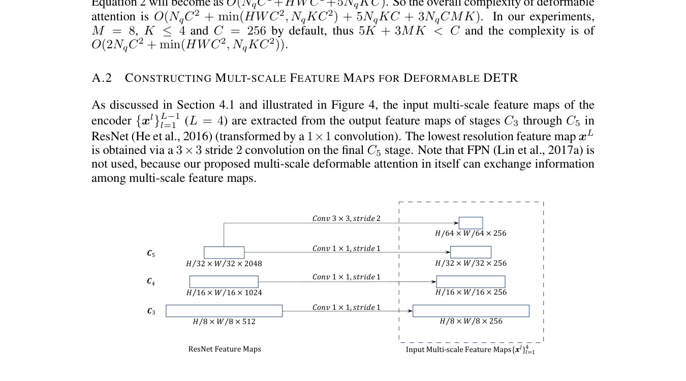
Figure 4: Constructing mult-scale feature maps for Deformable DETR.
图 4:为 Deformable DETR 构建多尺度特征图。
A.3 Bounding Box Prediction in Deformable DETR
A.3 Deformable DETR 中的边界框预测
Since the multi-scale deformable attention module extracts image features around the reference point, we design the detection head to predict the bounding box as relative offsets w.r.t. the reference point to further reduce the optimization difficulty. The reference point is used as the initial guess of the box center. The detection head predicts the relative offsets w.r.t. the reference point , i.e., , where are predicted by the detection head. and denote the and the function, respectively. The usage of and is to ensure is of normalized coordinates, as . In this way, the learned decoder attention will have strong correlation with the predicted bounding boxes, which also accelerates the training convergence.
由于多尺度可变形注意力在参考点周围提取图像特征,我们设计检测头把边界框预测为相对参考点的偏移,以进一步降低优化难度。参考点用作框中心的初始猜测。检测头预测相对参考点 的偏移,即 ,其中 由检测头预测。 与 分别表示 与逆 函数。使用二者是为确保 为归一化坐标,即 。如此,学到的解码器注意力将与预测边界框强相关,也加速训练收敛。
A.4 More Implementation Details
A.4 更多实现细节
Iterative Bounding Box Refinement. Here, each decoder layer refines the bounding boxes based on the predictions from the previous layer. Suppose there are number of decoder layers (e.g., ), given a normalized bounding box predicted by the -th decoder layer, the -th decoder layer refines the box as
迭代边界框精炼。 这里每个解码器层基于前一层预测精炼边界框。设解码器共 层(例如 ),给定第 层预测的归一化边界框 ,第 层按下式精炼:
where , are predicted at the -th decoder layer. Prediction heads for different decoder layers do not share parameters. The initial box is set as , , , and . The system is robust to the choice of and . We tried setting them as 0.05, 0.1, 0.2, 0.5, and achieved similar performance. To stabilize training, similar to Teed & Deng 2020, the gradients only back propagate through , and are blocked at .
其中 , 在第 层解码器预测。不同解码器层的预测头不共享参数。初始框设为 、、、。系统对 与 的选择稳健;我们试过 0.05、0.1、0.2、0.5,表现相近。为稳定训练,类似 Teed & Deng 2020,梯度仅经 反传,并在 处阻断。
In iterative bounding box refinement, for the -th decoder layer, we sample key elements respective to the box predicted from the -th decoder layer. For Equation 3 in the cross-attention module of the -th decoder layer, serves as the new reference point. The sampling offset is also modulated by the box size, as . Such modifications make the sampling locations related to the center and size of previously predicted boxes.
在迭代边界框精炼中,对第 层解码器,我们相对第 层预测的框 采样关键元素。对第 层交叉注意力中的式 3, 作为新参考点。采样偏移 也按框大小调制,为 。这些修改使采样位置与先前预测框的中心与尺寸相关。
Two-Stage Deformable DETR. In the first stage, given the output feature maps of the encoder, a detection head is applied to each pixel. The detection head is of a 3-layer FFN for bounding box regression, and a linear projection for bounding box binary classification (i.e., foreground and background), respectively. Let index a pixel from feature level with 2-d normalized coordinates , its corresponding bounding box is predicted by
两阶段 Deformable DETR。 第一阶段中,给定编码器输出特征图,对每个像素施加检测头。检测头分别为边界框回归的 3 层 FFN,以及边界框二分类(前景与背景)的线性投影。令 索引来自特征层 、二维归一化坐标为 的像素,其对应边界框预测为
where the base object scale is set as 0.05, are predicted by the bounding box regression branch. The Hungarian loss in DETR is used for training the detection head.
其中基础物体尺度 设为 0.05, 由边界框回归分支预测。检测头训练使用 DETR 中的 Hungarian 损失。
Given the predicted bounding boxes in the first stage, top scoring bounding boxes are picked as region proposals. In the second stage, these region proposals are fed into the decoder as initial boxes for the iterative bounding box refinement, where the positional embeddings of object queries are set as positional embeddings of region proposal coordinates.
给定第一阶段预测的边界框,取分数最高者作为区域提议。第二阶段把这些区域提议作为 迭代边界框精炼 的初始框送入解码器,物体查询的位置嵌入设为区域提议坐标的位置嵌入。
Initialization for Multi-scale Deformable Attention. In our experiments, the number of attention heads is set as . In multi-scale deformable attention modules, and are randomly initialized. Weight parameters of the linear projection for predicting and are initialized to zero. Bias parameters of the linear projection are initialized to make and () at initialization.
多尺度可变形注意力的初始化。 实验中注意力头数设为 。在多尺度可变形注意力模块中, 与 随机初始化。用于预测 与 的线性投影权重初始化为零。偏置初始化使初始化时 ,且 ()。
For iterative bounding box refinement, the initialized bias parameters for prediction in the decoder are further multiplied with , so that all the sampling points at initialization are within the corresponding bounding boxes predicted from the previous decoder layer.
对 迭代边界框精炼,解码器中 预测的初始化偏置再乘 ,使初始化时全部采样点落在前一层解码器预测的对应边界框内。
A.5 What Deformable DETR looks at?
A.5 Deformable DETR 在看什么?
For studying what Deformable DETR looks at to give final detection result, we draw the gradient norm of each item in final prediction (i.e., x/y coordinate of object center, width/height of object bounding box, category score of this object) with respect to each pixel in the image, as shown in Fig. 5. According to Taylor’s theorem, the gradient norm can reflect how much the output would be changed relative to the perturbation of the pixel, thus it could show us which pixels the model mainly relys on for predicting each item.
为研究 Deformable DETR 给出最终检测结果时看向何处,我们绘制最终预测中各项(即物体中心的 x/y 坐标、边界框宽/高、该物体类别分数)相对图像每个像素的梯度范数,如图 5 所示。根据泰勒定理,梯度范数可反映输出相对像素扰动会改变多少,从而显示模型预测各项主要依赖哪些像素。
The visualization indicates that Deformable DETR looks at extreme points of the object to determine its bounding box, which is similar to the observation in DETR (Carion et al. 2020). More concretely, Deformable DETR attends to left/right boundary of the object for x coordinate and width, and top/bottom boundary for y coordinate and height. Meanwhile, different to DETR (Carion et al. 2020), our Deformable DETR also looks at pixels inside the object for predicting its category.
可视化表明 Deformable DETR 通过关注物体极端点来确定边界框,与 DETR(Carion et al. 2020)中的观察类似。更具体地,对 x 坐标与宽度关注物体左/右边界,对 y 坐标与高度关注上/下边界。同时,与 DETR(Carion et al. 2020)不同,我们的 Deformable DETR 还会看向物体内部像素以预测类别。
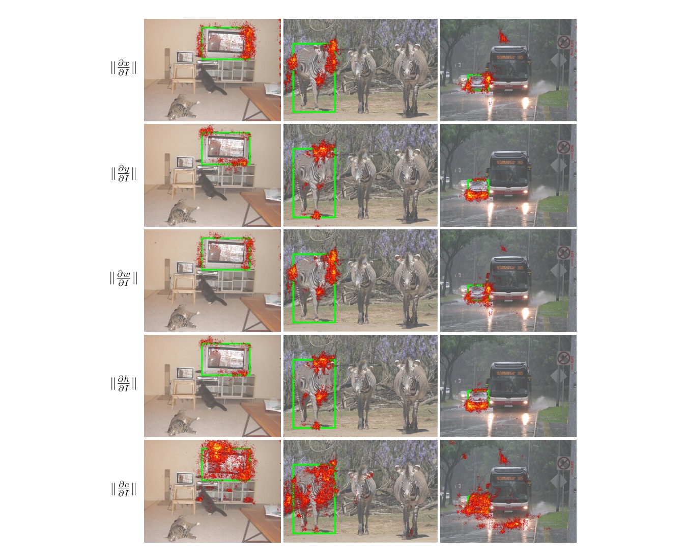
Figure 5: The gradient norm of each item (coordinate of object center , width/height of object bounding box , category score of this object) in final detection result with respect to each pixel in input image .
图 5:最终检测结果中各项(物体中心坐标 、边界框宽/高 、该物体类别分数 )相对输入图像 每个像素的梯度范数。
A.6 Visualization of Multi-scale Deformable Attention
A.6 多尺度可变形注意力可视化
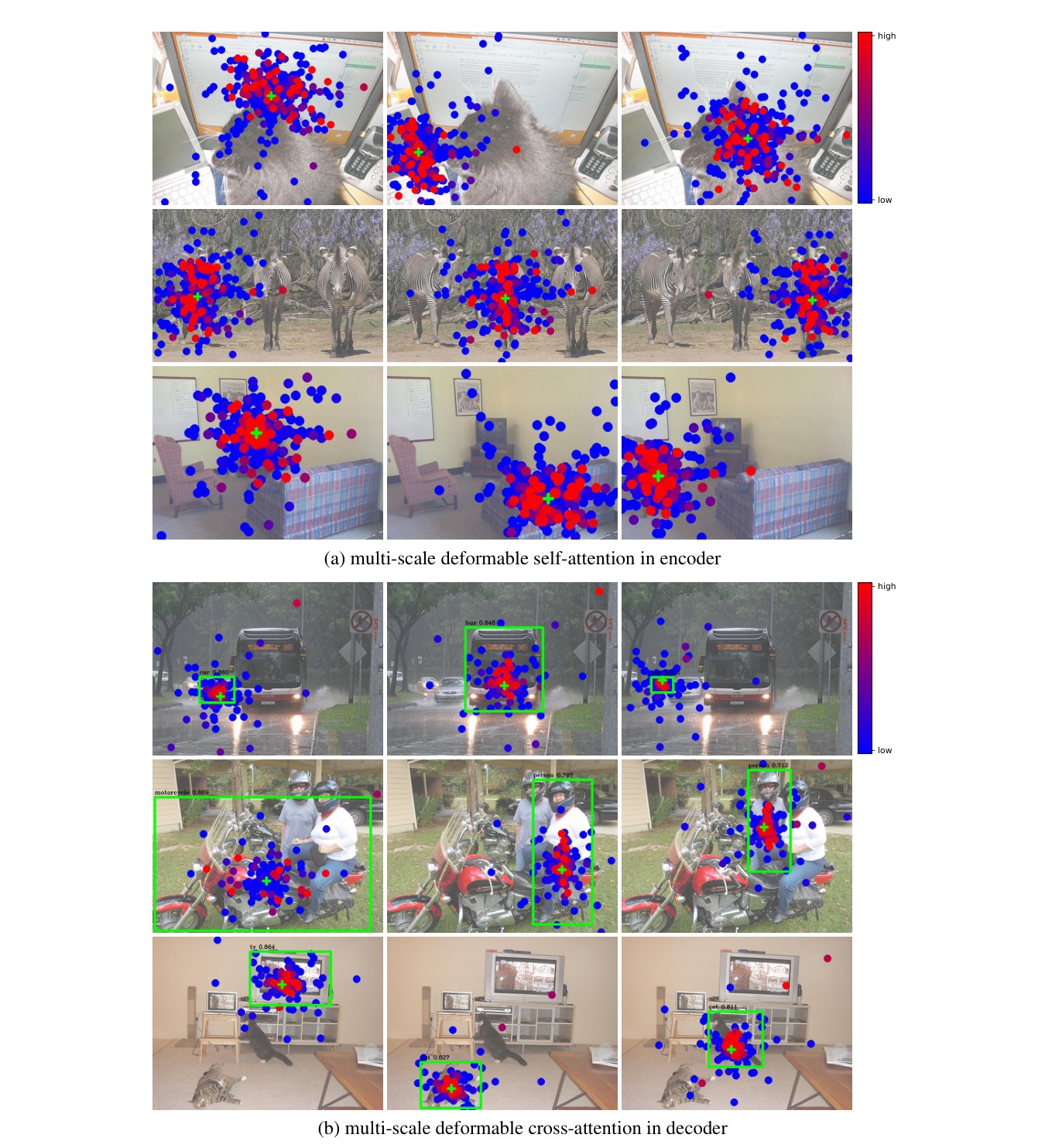
For better understanding learned multi-scale deformable attention modules, we visualize sampling points and attention weights of the last layer in encoder and decoder, as shown in Fig. 6. For readibility, we combine the sampling points and attention weights from feature maps of different resolutions into one picture.
为更好理解学到的多尺度可变形注意力模块,我们可视化编码器与解码器最后一层的采样点与注意力权重,如图 6 所示。为便于阅读,把不同分辨率特征图上的采样点与注意力权重合并到同一图中。
Similar to DETR (Carion et al. 2020), the instances are already separated in the encoder of Deformable DETR. While in the decoder, our model is focused on the whole foreground instance instead of only extreme points as observed in DETR (Carion et al. 2020). Combined with the visualization of in Fig. 5, we can guess the reason is that our Deformable DETR needs not only extreme points but also interior points to detemine object category. The visualization also demonstrates that the proposed multi-scale deformable attention module can adapt its sampling points and attention weights according to different scales and shapes of the foreground object.
与 DETR(Carion et al. 2020)类似,实例在 Deformable DETR 的编码器中已被分离。而在解码器中,我们的模型聚焦整块前景实例,而非如 DETR(Carion et al. 2020)所观察的那样仅关注极端点。结合图 5 中 的可视化,可猜测原因是:Deformable DETR 判定物体类别时既需要极端点,也需要内部点。可视化也表明,所提多尺度可变形注意力模块能按前景物体的不同尺度与形状自适应调整采样点与注意力权重。
(a) multi-scale deformable self-attention in encoder
(b) multi-scale deformable cross-attention in decoder
Figure 6: Visualization of multi-scale deformable attention. For readibility, we draw the sampling points and attention weights from feature maps of different resolutions in one picture. Each sampling point is marked as a filled circle whose color indicates its correspoinding attention weight. The reference point is shown as green cross marker, which is also equivalent to query point in encoder. In decoder, the predicted bounding box is shown as a green rectangle and the category and confidence score are texted just above it.
(a) 编码器中的多尺度可变形自注意力
(b) 解码器中的多尺度可变形交叉注意力
图 6:多尺度可变形注意力可视化。为便于阅读,我们把不同分辨率特征图上的采样点与注意力权重画在同一图中。每个采样点标为实心圆,颜色表示对应注意力权重。参考点标为绿色叉号,在编码器中也等价于查询点。在解码器中,预测边界框标为绿色矩形,类别与置信度写在其上方。
A.7 Notations
A.7 符号表
| Notation | Description |
|---|---|
| index for attention head | |
| index for feature level of key element | |
| index for query element | |
| index for key element | |
| number of query elements | |
| number of key elements | |
| number of attention heads | |
| number of input feature levels | |
| number of sampled keys in each feature level for each attention head | |
| input feature dimension | |
| feature dimension at each attention head | |
| height of input feature map | |
| width of input feature map | |
| height of input feature map of feature level | |
| width of input feature map of feature level | |
| attention weight of query to key at head | |
| attention weight of query to key in feature level at head | |
| input feature of query | |
| 2-d coordinate of reference point for query | |
| normalized 2-d coordinate of reference point for query | |
| input feature map (input feature of key elements) | |
| input feature of key | |
| input feature map of feature level | |
| sampling offset of query to key at head | |
| sampling offset of query to key in feature level at head | |
| output projection matrix at head | |
| input query projection matrix at head | |
| input key projection matrix at head | |
| input value projection matrix at head | |
| unnormalized 2-d coordinate of in feature level | |
| exponential function | |
| sigmoid function | |
| inverse sigmoid function |
Table 4: Lookup table for notations in the paper.
| 符号 | 说明 |
|---|---|
| 注意力头索引 | |
| 关键元素特征层索引 | |
| 查询元素索引 | |
| 关键元素索引 | |
| 查询元素数 | |
| 关键元素数 | |
| 注意力头数 | |
| 输入特征层数 | |
| 每个注意力头在每个特征层上的采样键数 | |
| 输入特征维 | |
| 每个注意力头的特征维 | |
| 输入特征图高度 | |
| 输入特征图宽度 | |
| 第 特征层输入特征图高度 | |
| 第 特征层输入特征图宽度 | |
| 第 头上第 查询对第 键的注意力权重 | |
| 第 头、第 特征层上第 查询对第 键的注意力权重 | |
| 第 查询的输入特征 | |
| 第 查询参考点的二维坐标 | |
| 第 查询参考点的归一化二维坐标 | |
| 输入特征图(关键元素的输入特征) | |
| 第 键的输入特征 | |
| 第 特征层的输入特征图 | |
| 第 头上第 查询对第 键的采样偏移 | |
| 第 头、第 特征层上第 查询对第 键的采样偏移 |
表:符号说明。