Encoder-Decoder with Atrous Separable Convolution for Semantic Image Segmentation
Encoder-Decoder with Atrous Separable Convolution for Semantic Image Segmentation
Liang-Chieh Chen Yukun Zhu George Papandreou Florian Schroff Hartwig Adam Affiliation: Google Inc. E-mail {lcchen, yukun, gpapan, fschroff, hadam}@google.com
Abstract
摘要
Spatial pyramid pooling module or encode-decoder structure are used in deep neural networks for semantic segmentation task. The former networks are able to encode multi-scale contextual information by probing the incoming features with filters or pooling operations at multiple rates and multiple effective fields-of-view, while the latter networks can capture sharper object boundaries by gradually recovering the spatial information. In this work, we propose to combine the advantages from both methods. Specifically, our proposed model, DeepLabv3+, extends DeepLabv3 by adding a simple yet effective decoder module to refine the segmentation results especially along object boundaries. We further explore the Xception model and apply the depthwise separable convolution to both Atrous Spatial Pyramid Pooling and decoder modules, resulting in a faster and stronger encoder-decoder network. We demonstrate the effectiveness of the proposed model on PASCAL VOC 2012 and Cityscapes datasets, achieving the test set performance of 89.0% and 82.1% without any post-processing. Our paper is accompanied with a publicly available reference implementation of the proposed models in Tensorflow at https://github.com/tensorflow/models/tree/master/research/deeplab.
空间金字塔池化模块或编码器–解码器结构,被用于语义分割任务的深度神经网络中。前者通过以多种膨胀率和多种有效感受野,用滤波器或池化操作探测输入特征,从而编码多尺度上下文信息;后者则通过逐步恢复空间信息,捕捉更锐利的物体边界。本文提出把这两种方法的优点结合起来。具体而言,我们提出的模型 DeepLabv3+ 扩展了 DeepLabv3,增加一个简单却有效的解码器模块,以细化分割结果,尤其是沿物体边界。我们进一步探索 Xception 模型,并把深度可分离卷积应用到空洞空间金字塔池化(ASPP)和解码器模块,从而得到一个更快、更强的编码器–解码器网络。我们在 PASCAL VOC 2012 和 Cityscapes 数据集上展示了提出模型的有效性,在不做任何后处理的情况下,测试集性能分别达到 89.0% 和 82.1%。本文附有所提模型在 Tensorflow 中的公开参考实现,地址为 https://github.com/tensorflow/models/tree/master/research/deeplab。
1 Introduction
1 引言
Keywords: Semantic image segmentation, spatial pyramid pooling, encoder-decoder, and depthwise separable convolution.
关键词:语义图像分割,空间金字塔池化,编码器–解码器,以及深度可分离卷积。
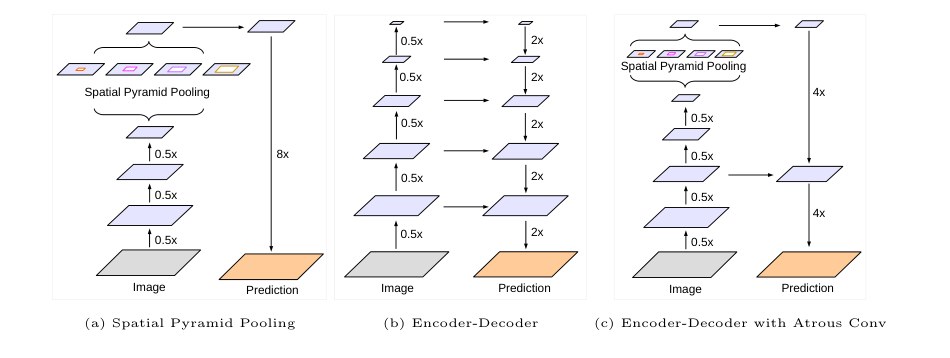
Figure 1: We improve DeepLabv3, which employs the spatial pyramid pooling module (a), with the encoder-decoder structure (b). The proposed model, DeepLabv3+, contains rich semantic information from the encoder module, while the detailed object boundaries are recovered by the simple yet effective decoder module. The encoder module allows us to extract features at an arbitrary resolution by applying atrous convolution.
图 1:我们用编码器–解码器结构(b)改进采用空间金字塔池化模块的 DeepLabv3(a)。提出的模型 DeepLabv3+ 从编码器模块获得丰富的语义信息,同时由简单却有效的解码器模块恢复细致的物体边界。编码器模块允许我们通过应用空洞卷积,在任意分辨率上抽取特征。
Semantic segmentation with the goal to assign semantic labels to every pixel in an image [1, 2, 3, 4, 5] is one of the fundamental topics in computer vision. Deep convolutional neural networks [6, 7, 8, 9, 10] based on the Fully Convolutional Neural Network [8, 11] show striking improvement over systems relying on hand-crafted features [12, 13, 14, 15, 16, 17] on benchmark tasks. In this work, we consider two types of neural networks that use spatial pyramid pooling module [18, 19, 20] or encoder-decoder structure [21, 22] for semantic segmentation, where the former one captures rich contextual information by pooling features at different resolution while the latter one is able to obtain sharp object boundaries.
语义分割的目标是给图像中的每个像素赋予语义标签 [1, 2, 3, 4, 5],是计算机视觉中的基本课题之一。基于全卷积网络 [8, 11] 的深度卷积神经网络 [6, 7, 8, 9, 10],在基准任务上相对依赖手工特征的系统 [12, 13, 14, 15, 16, 17] 表现出显著改进。本文考虑两类用于语义分割的神经网络:使用空间金字塔池化模块的 [18, 19, 20],以及使用编码器–解码器结构的 [21, 22]。前者通过在不同分辨率上池化特征来捕捉丰富的上下文信息,后者则能够得到锐利的物体边界。
In order to capture the contextual information at multiple scales, DeepLabv3 [23] applies several parallel atrous convolution with different rates (called Atrous Spatial Pyramid Pooling, or ASPP), while PSPNet [24] performs pooling operations at different grid scales. Even though rich semantic information is encoded in the last feature map, detailed information related to object boundaries is missing due to the pooling or convolutions with striding operations within the network backbone. This could be alleviated by applying the atrous convolution to extract denser feature maps. However, given the design of state-of-art neural networks [7, 9, 10, 25, 26] and limited GPU memory, it is computationally prohibitive to extract output feature maps that are 8, or even 4 times smaller than the input resolution. Taking ResNet-101 [25] for example, when applying atrous convolution to extract output features that are 16 times smaller than input resolution, features within the last 3 residual blocks (9 layers) have to be dilated. Even worse, 26 residual blocks (78 layers!) will be affected if output features that are 8 times smaller than input are desired. Thus, it is computationally intensive if denser output features are extracted for this type of models. On the other hand, encoder-decoder models [21, 22] lend themselves to faster computation (since no features are dilated) in the encoder path and gradually recover sharp object boundaries in the decoder path. Attempting to combine the advantages from both methods, we propose to enrich the encoder module in the encoder-decoder networks by incorporating the multi-scale contextual information.
为了捕捉多个尺度上的上下文信息,DeepLabv3 [23] 并行应用若干种不同膨胀率的空洞卷积(称为空洞空间金字塔池化,ASPP),而 PSPNet [24] 则在不同网格尺度上做池化。尽管最后一张特征图中编码了丰富的语义信息,但由于网络主干中的池化或带步长的卷积操作,与物体边界相关的细节信息会丢失。这可以通过应用空洞卷积来抽取更密的特征图加以缓解。不过,鉴于当时最好的神经网络的设计 [7, 9, 10, 25, 26] 以及有限的 GPU 内存,要抽取比输入分辨率小 8 倍、甚至 4 倍的输出特征图,在计算上是难以承受的。以 ResNet-101 [25] 为例,当应用空洞卷积抽取比输入分辨率小 16 倍的输出特征时,最后 3 个残差块(9 层)内的特征必须被膨胀。更糟的是,如果希望得到比输入小 8 倍的输出特征,将有 26 个残差块(78 层!)受到影响。因此,对这类模型抽取更密的输出特征,计算量很大。另一方面,编码器–解码器模型 [21, 22] 便于在编码器路径中更快计算(因为没有特征被膨胀),并在解码器路径中逐步恢复锐利的物体边界。为尝试结合两种方法的优点,我们提出在编码器–解码器网络的编码器模块中纳入多尺度上下文信息,以丰富编码器。
In particular, our proposed model, called DeepLabv3+, extends DeepLabv3 [23] by adding a simple yet effective decoder module to recover the object boundaries, as illustrated in Fig. 1. The rich semantic information is encoded in the output of DeepLabv3, with atrous convolution allowing one to control the density of the encoder features, depending on the budget of computation resources. Furthermore, the decoder module allows detailed object boundary recovery.
具体而言,我们提出的模型称为 DeepLabv3+,它通过增加一个简单却有效的解码器模块来恢复物体边界,从而扩展 DeepLabv3 [23],如图 1 所示。丰富的语义信息编码在 DeepLabv3 的输出中,空洞卷积则允许人们按计算资源预算控制编码器特征的密度。此外,解码器模块允许细致地恢复物体边界。
Motivated by the recent success of depthwise separable convolution [27, 28, 26, 29, 30], we also explore this operation and show improvement in terms of both speed and accuracy by adapting the Xception model [26], similar to [31], for the task of semantic segmentation, and applying the atrous separable convolution to both the ASPP and decoder modules. Finally, we demonstrate the effectiveness of the proposed model on PASCAL VOC 2012 and Cityscapes datasts and attain the test set performance of 89.0% and 82.1% without any post-processing, setting a new state-of-the-art.
受深度可分离卷积近期成功的启发 [27, 28, 26, 29, 30],我们也探索这一操作,并通过为语义分割任务改编 Xception 模型 [26](做法类似 [31]),以及把空洞可分离卷积应用到 ASPP 和解码器模块,展示了速度和精度上的改进。最后,我们在 PASCAL VOC 2012 和 Cityscapes 数据集上展示提出模型的有效性,在不做任何后处理的情况下,测试集性能分别达到 89.0% 和 82.1%,树立了新的当时最好水平。
In summary, our contributions are:
概括起来,我们的贡献是:
- • We propose a novel encoder-decoder structure which employs DeepLabv3 as a powerful encoder module and a simple yet effective decoder module.
- • 我们提出一种新颖的编码器–解码器结构,用 DeepLabv3 作为强大的编码器模块,并配以一个简单却有效的解码器模块。
- • In our structure, one can arbitrarily control the resolution of extracted encoder features by atrous convolution to trade-off precision and runtime, which is not possible with existing encoder-decoder models.
- • 在我们的结构中,可以通过空洞卷积任意控制所抽取编码器特征的分辨率,以在精度和运行时间之间权衡,这是现有编码器–解码器模型做不到的。
- • We adapt the Xception model for the segmentation task and apply depthwise separable convolution to both ASPP module and decoder module, resulting in a faster and stronger encoder-decoder network.
- • 我们为分割任务改编 Xception 模型,并把深度可分离卷积应用到 ASPP 模块和解码器模块,从而得到一个更快、更强的编码器–解码器网络。
- • Our proposed model attains a new state-of-art performance on PASCAL VOC 2012 and Cityscapes datasets. We also provide detailed analysis of design choices and model variants.
- • 我们提出的模型在 PASCAL VOC 2012 和 Cityscapes 数据集上达到了新的当时最好性能。我们还对设计选择和模型变体做了详细分析。
- • We make our Tensorflow-based implementation of the proposed model publicly available at https://github.com/tensorflow/models/tree/master/research/deeplab.
- • 我们把提出模型基于 Tensorflow 的实现公开在 https://github.com/tensorflow/models/tree/master/research/deeplab。
2 Related Work
2 相关工作
Models based on Fully Convolutional Networks (FCNs) [8, 11] have demonstrated significant improvement on several segmentation benchmarks [1, 2, 3, 4, 5]. There are several model variants proposed to exploit the contextual information for segmentation [12, 13, 14, 15, 16, 17, 32, 33], including those that employ multi-scale inputs (i.e., image pyramid) [34, 35, 36, 37, 38, 39] or those that adopt probabilistic graphical models (such as DenseCRF [40] with efficient inference algorithm [41]) [42, 43, 44, 37, 45, 46, 47, 48, 49, 50, 51, 39]. In this work, we mainly discuss about the models that use spatial pyramid pooling and encoder-decoder structure.
基于全卷积网络(FCN)[8, 11] 的模型,已在若干分割基准上展示出显著改进 [1, 2, 3, 4, 5]。已有若干模型变体被提出,以利用上下文信息做分割 [12, 13, 14, 15, 16, 17, 32, 33],包括采用多尺度输入(即图像金字塔)的 [34, 35, 36, 37, 38, 39],以及采用概率图模型(例如带高效推断算法 [41] 的 DenseCRF [40])的 [42, 43, 44, 37, 45, 46, 47, 48, 49, 50, 51, 39]。本文主要讨论使用空间金字塔池化和编码器–解码器结构的模型。
Spatial pyramid pooling: Models, such as PSPNet [24] or DeepLab [39, 23], perform spatial pyramid pooling [18, 19] at several grid scales (including image-level pooling [52]) or apply several parallel atrous convolution with different rates (called Atrous Spatial Pyramid Pooling, or ASPP). These models have shown promising results on several segmentation benchmarks by exploiting the multi-scale information.
空间金字塔池化: 诸如 PSPNet [24] 或 DeepLab [39, 23] 这样的模型,在若干网格尺度上做空间金字塔池化 [18, 19](包括图像级池化 [52]),或并行应用若干种不同膨胀率的空洞卷积(称为空洞空间金字塔池化,ASPP)。这些模型通过利用多尺度信息,已在若干分割基准上展示出有前景的结果。
Encoder-decoder: The encoder-decoder networks have been successfully applied to many computer vision tasks, including human pose estimation [53], object detection [54, 55, 56], and semantic segmentation [11, 57, 21, 22, 58, 59, 60, 61, 62, 63, 64]. Typically, the encoder-decoder networks contain (1) an encoder module that gradually reduces the feature maps and captures higher semantic information, and (2) a decoder module that gradually recovers the spatial information. Building on top of this idea, we propose to use DeepLabv3 [23] as the encoder module and add a simple yet effective decoder module to obtain sharper segmentations.
编码器–解码器: 编码器–解码器网络已被成功应用于许多计算机视觉任务,包括人体姿态估计 [53]、物体检测 [54, 55, 56] 以及语义分割 [11, 57, 21, 22, 58, 59, 60, 61, 62, 63, 64]。典型地,编码器–解码器网络包含(1)一个逐渐减小特征图并捕捉更高层语义信息的编码器模块,以及(2)一个逐渐恢复空间信息的解码器模块。基于这一想法,我们提出用 DeepLabv3 [23] 作为编码器模块,并增加一个简单却有效的解码器模块,以得到更锐利的分割。
Depthwise separable convolution: Depthwise separable convolution [27, 28] or group convolution [7, 65], a powerful operation to reduce the computation cost and number of parameters while maintaining similar (or slightly better) performance. This operation has been adopted in many recent neural network designs [66, 67, 26, 29, 30, 31, 68]. In particular, we explore the Xception model [26], similar to [31] for their COCO 2017 detection challenge submission, and show improvement in terms of both accuracy and speed for the task of semantic segmentation.
深度可分离卷积: 深度可分离卷积 [27, 28] 或分组卷积 [7, 65],是一种在保持相似(或略更好)性能的同时,降低计算代价和参数数量的有力操作。这一操作已被许多近期神经网络设计所采用 [66, 67, 26, 29, 30, 31, 68]。尤其是,我们探索 Xception 模型 [26],做法类似于 [31] 在其 COCO 2017 检测挑战提交中的改法,并展示了在语义分割任务上精度和速度的改进。
3 Methods
3 方法
In this section, we briefly introduce atrous convolution [69, 70, 8, 71, 42] and depthwise separable convolution [27, 28, 67, 26, 29]. We then review DeepLabv3 [23] which is used as our encoder module before discussing the proposed decoder module appended to the encoder output. We also present a modified Xception model [26, 31] which further improves the performance with faster computation.
本节我们简要介绍空洞卷积 [69, 70, 8, 71, 42] 和深度可分离卷积 [27, 28, 67, 26, 29]。然后回顾被用作编码器模块的 DeepLabv3 [23],再讨论接到编码器输出上的提出解码器模块。我们也给出一个改进的 Xception 模型 [26, 31],它以更快的计算进一步改进了性能。
3.1 Encoder-Decoder with Atrous Convolution
3.1 带空洞卷积的编码器–解码器
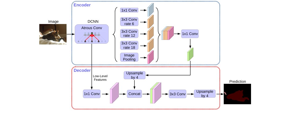
Figure 2: Our proposed DeepLabv3+ extends DeepLabv3 by employing a encoder-decoder structure. The encoder module encodes multi-scale contextual information by applying atrous convolution at multiple scales, while the simple yet effective decoder module refines the segmentation results along object boundaries.
图 2:我们提出的 DeepLabv3+ 通过采用编码器–解码器结构来扩展 DeepLabv3。编码器模块通过在多个尺度上应用空洞卷积来编码多尺度上下文信息,而简单却有效的解码器模块则沿物体边界细化分割结果。
Atrous convolution: Atrous convolution, a powerful tool that allows us to explicitly control the resolution of features computed by deep convolutional neural networks and adjust filter’s field-of-view in order to capture multi-scale information, generalizes standard convolution operation. In the case of two-dimensional signals, for each location on the output feature map and a convolution filter , atrous convolution is applied over the input feature map as follows:
空洞卷积: 空洞卷积是一种有力的工具,它允许我们显式控制深度卷积神经网络所计算特征的分辨率,并调整滤波器的感受野以捕捉多尺度信息,是对标准卷积操作的推广。对二维信号,对输出特征图 上的每个位置 以及卷积滤波器 ,空洞卷积在输入特征图 上按如下方式应用:
where the atrous rate r determines the stride with which we sample the input signal. We refer interested readers to [39] for more details. Note that standard convolution is a special case in which rate . The filter’s field-of-view is adaptively modified by changing the rate value.
其中空洞率 r 决定我们对输入信号抽样的步长。更多细节请参阅 [39]。注意,标准卷积是膨胀率 的特殊情形。滤波器的感受野通过改变膨胀率而被自适应地修改。
Depthwise separable convolution: Depthwise separable convolution, factorizing a standard convolution into a depthwise convolution followed by a pointwise convolution (i.e., convolution), drastically reduces computation complexity. Specifically, the depthwise convolution performs a spatial convolution independently for each input channel, while the pointwise convolution is employed to combine the output from the depthwise convolution. In the TensorFlow [72] implementation of depthwise separable convolution, atrous convolution has been supported in the depthwise convolution (i.e., the spatial convolution), as illustrated in Fig. 3. In this work, we refer the resulting convolution as atrous separable convolution, and found that atrous separable convolution significantly reduces the computation complexity of proposed model while maintaining similar (or better) performance.
深度可分离卷积: 深度可分离卷积把标准卷积分解为一次深度卷积再接一次逐点卷积(即 卷积),从而大幅降低计算复杂度。具体而言,深度卷积对每个输入通道独立地做空间卷积,而逐点卷积被用来组合深度卷积的输出。在 TensorFlow [72] 对深度可分离卷积的实现中,空洞卷积已在深度卷积(即空间卷积)中得到支持,如图 3 所示。在本文中,我们把得到的卷积称为空洞可分离卷积,并发现空洞可分离卷积在保持相似(或更好)性能的同时,显著降低了提出模型的计算复杂度。
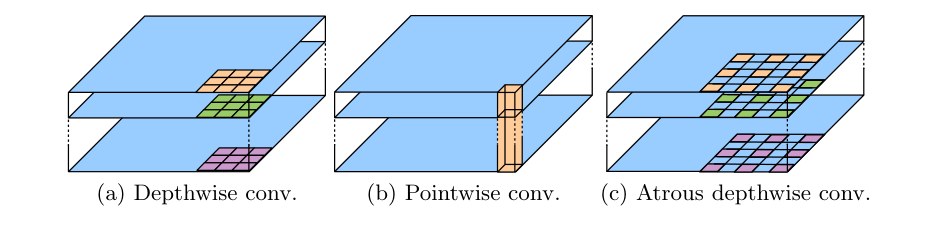
Figure 3: Depthwise separable convolution decomposes a standard convolution into (a) a depthwise convolution (applying a single filter for each input channel) and (b) a pointwise convolution (combining the outputs from depthwise convolution across channels). In this work, we explore atrous separable convolution where atrous convolution is adopted in the depthwise convolution, as shown in (c) with .
图 3: 深度可分离卷积把标准卷积分解为(a)一次深度卷积(对每个输入通道应用一个滤波器)和(b)一次逐点卷积(跨通道组合深度卷积的输出)。本文中,我们探索空洞可分离卷积,即在深度卷积中采用空洞卷积,如(c)所示,其中 。
DeepLabv3 as encoder: DeepLabv3 [23] employs atrous convolution [69, 70, 8, 71] to extract the features computed by deep convolutional neural networks at an arbitrary resolution. Here, we denote as the ratio of input image spatial resolution to the final output resolution (before global pooling or fully-connected layer). For the task of image classification, the spatial resolution of the final feature maps is usually 32 times smaller than the input image resolution and thus . For the task of semantic segmentation, one can adopt (or ) for denser feature extraction by removing the striding in the last one (or two) block(s) and applying the atrous convolution correspondingly (e.g., we apply and to the last two blocks respectively for ). Additionally, DeepLabv3 augments the Atrous Spatial Pyramid Pooling module, which probes convolutional features at multiple scales by applying atrous convolution with different rates, with the image-level features [52]. We use the last feature map before logits in the original DeepLabv3 as the encoder output in our proposed encoder-decoder structure. Note the encoder output feature map contains 256 channels and rich semantic information. Besides, one could extract features at an arbitrary resolution by applying the atrous convolution, depending on the computation budget.
以 DeepLabv3 作为编码器: DeepLabv3 [23] 采用空洞卷积 [69, 70, 8, 71],以任意分辨率抽取深度卷积神经网络所计算的特征。这里,我们把 (输出步长)记为输入图像空间分辨率与最终输出分辨率(在全局池化或全连接层之前)之比。对图像分类任务,最终特征图的空间分辨率通常比输入图像分辨率小 32 倍,因而 。对语义分割任务,可以通过去掉最后一块(或两块)中的步长,并相应地应用空洞卷积,采用 (或 )以抽取更密的特征(例如,对 ,我们分别对最后两块应用 和 )。此外,DeepLabv3 用图像级特征 [52] 增强空洞空间金字塔池化模块,该模块通过应用不同膨胀率的空洞卷积,在多个尺度上探测卷积特征。在我们提出的编码器–解码器结构中,我们把原版 DeepLabv3 中 logits 之前的最后一张特征图用作编码器输出。注意,编码器输出特征图包含 256 个通道以及丰富的语义信息。此外,人们可以视计算预算,通过应用空洞卷积在任意分辨率上抽取特征。
Proposed decoder: The encoder features from DeepLabv3 are usually computed with . In the work of [23], the features are bilinearly upsampled by a factor of 16, which could be considered a naive decoder module. However, this naive decoder module may not successfully recover object segmentation details. We thus propose a simple yet effective decoder module, as illustrated in Fig. 2. The encoder features are first bilinearly upsampled by a factor of 4 and then concatenated with the corresponding low-level features [73] from the network backbone that have the same spatial resolution (e.g., Conv2 before striding in ResNet-101 [25]). We apply another convolution on the low-level features to reduce the number of channels, since the corresponding low-level features usually contain a large number of channels (e.g., 256 or 512) which may outweigh the importance of the rich encoder features (only 256 channels in our model) and make the training harder. After the concatenation, we apply a few convolutions to refine the features followed by another simple bilinear upsampling by a factor of 4. We show in Sec. 4 that using for the encoder module strikes the best trade-off between speed and accuracy. The performance is marginally improved when using for the encoder module at the cost of extra computation complexity.
提出的解码器: 来自 DeepLabv3 的编码器特征通常以 计算。在 [23] 的工作中,特征被双线性上采样 16 倍,这可以视为一个朴素的解码器模块。不过,这种朴素解码器模块可能无法成功地恢复物体分割细节。因此我们提出一个简单却有效的解码器模块,如图 2 所示。编码器特征先被双线性上采样 4 倍,再与网络主干中具有相同空间分辨率的相应浅层特征 [73] 拼接(例如 ResNet-101 [25] 中步长之前的 Conv2)。我们在浅层特征上再应用一次 卷积以降低通道数,因为相应的浅层特征通常包含大量通道(例如 256 或 512),可能会压过丰富编码器特征的重要性(在我们的模型中只有 256 个通道),并使训练更困难。拼接之后,我们应用几次 卷积来细化特征,然后再做一次简单的 4 倍双线性上采样。我们在第 4 节中表明,编码器模块使用 在速度和精度之间取得了最好的权衡。当编码器模块使用 时,性能只有边际改进,代价则是额外的计算复杂度。
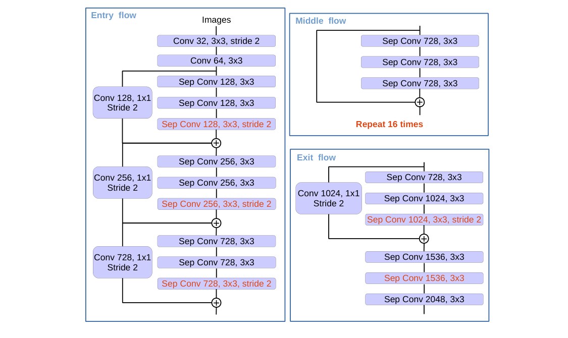
Figure 4: We modify the Xception as follows: (1) more layers (same as MSRA’s modification except the changes in Entry flow), (2) all the max pooling operations are replaced by depthwise separable convolutions with striding, and (3) extra batch normalization and ReLU are added after each depthwise convolution, similar to MobileNet.
图 4:我们按如下方式修改 Xception:(1)层数更多(与 MSRA 的修改相同,但入口流有改动),(2)所有最大池化操作都换成带步长的深度可分离卷积,以及(3)在每个 深度卷积之后额外加入批归一化和 ReLU,类似于 MobileNet。
3.2 Modified Aligned Xception
3.2 改进的 Aligned Xception
The Xception model [26] has shown promising image classification results on ImageNet [74] with fast computation. More recently, the MSRA team [31] modifies the Xception model (called Aligned Xception) and further pushes the performance in the task of object detection. Motivated by these findings, we work in the same direction to adapt the Xception model for the task of semantic image segmentation. In particular, we make a few more changes on top of MSRA’s modifications, namely (1) deeper Xception same as in [31] except that we do not modify the entry flow network structure for fast computation and memory efficiency, (2) all max pooling operations are replaced by depthwise separable convolution with striding, which enables us to apply atrous separable convolution to extract feature maps at an arbitrary resolution (another option is to extend the atrous algorithm to max pooling operations), and (3) extra batch normalization [75] and ReLU activation are added after each depthwise convolution, similar to MobileNet design [29]. See Fig. 4 for details.
Xception 模型 [26] 已在 ImageNet [74] 上展示出有前景的图像分类结果,且计算很快。更近一些,MSRA 团队 [31] 修改了 Xception 模型(称为 Aligned Xception),并在物体检测任务上进一步推高了性能。受这些发现启发,我们沿同一方向为语义图像分割任务改编 Xception 模型。具体而言,我们在 MSRA 的修改之上又做了几处改动,即(1)Xception 加深的方式与 [31] 相同,但为了快速计算和节省内存,我们并不修改入口流的网络结构;(2)所有最大池化操作都换成带步长的深度可分离卷积,这使我们能够应用空洞可分离卷积,在任意分辨率上抽取特征图(另一种选择是把空洞算法扩展到最大池化操作);以及(3)在每个 深度卷积之后额外加入批归一化 [75] 和 ReLU 激活,类似于 MobileNet 的设计 [29]。细节见图 4。
4 Experimental Evaluation
4 实验评估
We employ ImageNet-1k [74] pretrained ResNet-101 [25] or modified aligned Xception [26, 31] to extract dense feature maps by atrous convolution. Our implementation is built on TensorFlow [72] and is made publicly available.
我们采用在 ImageNet-1k [74] 上预训练的 ResNet-101 [25] 或改进的 aligned Xception [26, 31],通过空洞卷积抽取稠密特征图。我们的实现建立在 TensorFlow [72] 上,并且已经公开。
The proposed models are evaluated on the PASCAL VOC 2012 semantic segmentation benchmark [1] which contains 20 foreground object classes and one background class. The original dataset contains (train), (val), and (test) pixel-level annotated images. We augment the dataset by the extra annotations provided by [76], resulting in (trainaug) training images. The performance is measured in terms of pixel intersection-over-union averaged across the 21 classes (mIOU).
提出的模型在 PASCAL VOC 2012 语义分割基准 [1] 上评估,该基准包含 20 个前景物体类别和一个背景类。原始数据集含有 (train)、(val)和 (test)张像素级标注图像。我们用 [76] 提供的额外标注扩充数据集,得到 (trainaug)张训练图像。性能用 21 类上平均的像素交并比(mIOU)来度量。
We follow the same training protocol as in [23] and refer the interested readers to [23] for details. In short, we employ the same learning rate schedule (i.e., “poly” policy [52] and same initial learning rate ), crop size , fine-tuning batch normalization parameters [75] when , and random scale data augmentation during training. Note that we also include batch normalization parameters in the proposed decoder module. Our proposed model is trained end-to-end without piecewise pretraining of each component.
我们遵循与 [23] 相同的训练规程,细节请参阅 [23]。简而言之,我们采用相同的学习率日程(即 “poly” 策略 [52] 以及相同的初始学习率 )、裁剪大小 ,在 时微调批归一化参数 [75],并在训练中使用随机尺度数据增强。注意,我们也把批归一化参数纳入提出的解码器模块。我们提出的模型是端到端训练的,并不对各组件做分段预训练。
4.1 Decoder Design Choices
4.1 解码器的设计选择
We define “DeepLabv3 feature map” as the last feature map computed by DeepLabv3 (i.e., the features containing ASPP features and image-level features), and as a convolution operation with kernel and filters.
我们把 “DeepLabv3 特征图” 定义为由 DeepLabv3 计算出的最后一张特征图(即包含 ASPP 特征和图像级特征的那些特征),并把 定义为核为 、滤波器数为 的卷积操作。
When employing , ResNet-101 based DeepLabv3 [23] bilinearly upsamples the logits by during both training and evaluation. This simple bilinear upsampling could be considered as a naive decoder design, attaining the performance of [23] on PASCAL VOC 2012 val set and is better than not using this naive decoder during training (i.e., downsampling groundtruth during training). To improve over this naive baseline, our proposed model “DeepLabv3+” adds the decoder module on top of the encoder output, as shown in Fig. 2. In the decoder module, we consider three places for different design choices, namely (1) the convolution used to reduce the channels of the low-level feature map from the encoder module, (2) the convolution used to obtain sharper segmentation results, and (3) what encoder low-level features should be used.
当采用 时,基于 ResNet-101 的 DeepLabv3 [23] 在训练和评估时都把 logits 双线性上采样 倍。这种简单的双线性上采样可以视为一种朴素的解码器设计,在 PASCAL VOC 2012 val 集上达到 的性能 [23],比训练时不使用这一朴素解码器(即训练时对真值做下采样)好 。为改进这一朴素基线,我们提出的模型 “DeepLabv3+” 在编码器输出之上增加解码器模块,如图 2 所示。在解码器模块中,我们考虑三处不同的设计选择,即(1)用来降低编码器模块浅层特征图通道数的 卷积,(2)用来得到更锐利分割结果的 卷积,以及(3)应当使用哪些编码器浅层特征。
To evaluate the effect of the convolution in the decoder module, we employ and the Conv2 features from ResNet-101 network backbone, i.e., the last feature map in res2x residual block (to be concrete, we use the feature map before striding). As shown in Tab. 1, reducing the channels of the low-level feature map from the encoder module to either 48 or 32 leads to better performance. We thus adopt for channel reduction.
为评估解码器模块中 卷积的效果,我们采用 以及来自 ResNet-101 网络主干的 Conv2 特征,即 res2x 残差块中的最后一张特征图(具体来说,我们使用步长之前的特征图)。如表 1 所示,把编码器模块浅层特征图的通道降到 48 或 32,会带来更好的性能。因此我们采用 来降低通道数。
We then design the convolution structure for the decoder module and report the findings in Tab. 2. We find that after concatenating the Conv2 feature map (before striding) with DeepLabv3 feature map, it is more effective to employ two convolution with 256 filters than using simply one or three convolutions. Changing the number of filters from 256 to 128 or the kernel size from to degrades performance. We also experiment with the case where both Conv2 and Conv3 feature maps are exploited in the decoder module. In this case, the decoder feature map are gradually upsampled by 2, concatenated with Conv3 first and then Conv2, and each will be refined by the operation. The whole decoding procedure is then similar to the U-Net/SegNet design [21, 22]. However, we have not observed significant improvement. Thus, in the end, we adopt the very simple yet effective decoder module: the concatenation of the DeepLabv3 feature map and the channel-reduced Conv2 feature map are refined by two operations. Note that our proposed DeepLabv3+ model has . We do not pursue further denser output feature map (i.e., ) given the limited GPU resources.
然后我们为解码器模块设计 卷积结构,并在表 2 中报告发现。我们发现,在把 Conv2 特征图(步长之前)与 DeepLabv3 特征图拼接之后,采用两次带 256 个滤波器的 卷积,比只用一次或三次卷积更有效。把滤波器数从 256 改成 128,或把核大小从 改成 ,都会降低性能。我们也实验了在解码器模块中同时利用 Conv2 和 Conv3 特征图的情形。此时,解码器特征图逐渐上采样 2 倍,先与 Conv3 拼接,再与 Conv2 拼接,并且每一处都由 操作细化。整个解码过程于是类似于 U-Net/SegNet 的设计 [21, 22]。不过,我们并未观察到显著改进。因此,最终我们采用非常简单却有效的解码器模块:DeepLabv3 特征图与通道已降低的 Conv2 特征图的拼接,由两次 操作细化。注意,我们提出的 DeepLabv3+ 模型具有 。鉴于有限的 GPU 资源,我们不再追求更密的输出特征图(即 )。
| Channels | 8 | 16 | 32 | 48 | 64 |
|---|---|---|---|---|---|
| mIOU | 77.61% | 77.92% | 78.16% | 78.21% | 77.94% |
Table 1: PASCAL VOC 2012 val set. Effect of decoder convolution used to reduce the channels of low-level feature map from the encoder module. We fix the other components in the decoder structure as using and Conv2.
| 通道数 | 8 | 16 | 32 | 48 | 64 |
|---|---|---|---|---|---|
| mIOU | 77.61% | 77.92% | 78.16% | 78.21% | 77.94% |
表 1:PASCAL VOC 2012 val 集。解码器中用于降低编码器模块浅层特征图通道数的 卷积的影响。我们把解码器结构中的其余组件固定为使用 和 Conv2。
| Features | Conv | mIOU | |
|---|---|---|---|
| Conv2 | Conv3 | Structure | |
| ✓ | 78.21% | ||
| ✓ | 78.85% | ||
| ✓ | 78.02% | ||
| ✓ | 77.25% | ||
| ✓ | 78.07% | ||
| ✓ | ✓ | 78.61% |
Table 2: Effect of decoder structure when fixing to reduce the encoder feature channels. We found that it is most effective to use the Conv2 (before striding) feature map and two extra operations. Performance on VOC 2012 val set.
| 特征 | 卷积 | mIOU | |
|---|---|---|---|
| Conv2 | Conv3 | 结构 | |
| ✓ | 78.21% | ||
| ✓ | 78.85% | ||
| ✓ | 78.02% | ||
| ✓ | 77.25% | ||
| ✓ | 78.07% | ||
| ✓ | ✓ | 78.61% |
表 2:在固定用 降低编码器特征通道数时,解码器结构的影响。我们发现,使用 Conv2(步长之前)特征图并再加两次 操作最为有效。性能在 VOC 2012 val 集上报告。
| Encoder | Decoder | MS | Flip | mIOU | Multiply-Adds | |
|---|---|---|---|---|---|---|
| train OS | eval OS | |||||
| 16 | 16 | 77.21% | 81.02B | |||
| 16 | 8 | 78.51% | 276.18B | |||
| 16 | 8 | ✓ | 79.45% | 2435.37B | ||
| 16 | 8 | ✓ | ✓ | 79.77% | 4870.59B | |
| 16 | 16 | ✓ | 78.85% | 101.28B | ||
| 16 | 16 | ✓ | ✓ | 80.09% | 898.69B | |
| 16 | 16 | ✓ | ✓ | ✓ | 80.22% | 1797.23B |
| 16 | 8 | ✓ | 79.35% | 297.92B | ||
| 16 | 8 | ✓ | ✓ | 80.43% | 2623.61B | |
| 16 | 8 | ✓ | ✓ | ✓ | 80.57% | 5247.07B |
| 32 | 32 | 75.43% | 52.43B | |||
| 32 | 32 | ✓ | 77.37% | 74.20B | ||
| 32 | 16 | ✓ | 77.80% | 101.28B | ||
| 32 | 8 | ✓ | 77.92% | 297.92B |
Table 3: Inference strategy on the PASCAL VOC 2012 val set using ResNet-101. train OS: The used during training. eval OS: The used during evaluation. Decoder: Employing the proposed decoder structure. MS: Multi-scale inputs during evaluation. Flip: Adding left-right flipped inputs.
| 编码器 | 解码器 | MS | Flip | mIOU | 乘加次数 | |
|---|---|---|---|---|---|---|
| train OS | eval OS | |||||
| 16 | 16 | 77.21% | 81.02B | |||
| 16 | 8 | 78.51% | 276.18B | |||
| 16 | 8 | ✓ | 79.45% | 2435.37B | ||
| 16 | 8 | ✓ | ✓ | 79.77% | 4870.59B | |
| 16 | 16 | ✓ | 78.85% | 101.28B | ||
| 16 | 16 | ✓ | ✓ | 80.09% | 898.69B | |
| 16 | 16 | ✓ | ✓ | ✓ | 80.22% | 1797.23B |
| 16 | 8 | ✓ | 79.35% | 297.92B | ||
| 16 | 8 | ✓ | ✓ | 80.43% | 2623.61B | |
| 16 | 8 | ✓ | ✓ | ✓ | 80.57% | 5247.07B |
| 32 | 32 | 75.43% | 52.43B | |||
| 32 | 32 | ✓ | 77.37% | 74.20B | ||
| 32 | 16 | ✓ | 77.80% | 101.28B | ||
| 32 | 8 | ✓ | 77.92% | 297.92B |
表 3:在使用 ResNet-101 时,PASCAL VOC 2012 val 集上的推断策略。train OS:训练时使用的 。eval OS:评估时使用的 。Decoder:采用提出的解码器结构。MS:评估时使用多尺度输入。Flip:加入左右翻转的输入。
4.2 ResNet-101 as Network Backbone
4.2 以 ResNet-101 作为网络主干
To compare the model variants in terms of both accuracy and speed, we report mIOU and Multiply-Adds in Tab. 3 when using ResNet-101 [25] as network backbone in the proposed DeepLabv3+ model. Thanks to atrous convolution, we are able to obtain features at different resolutions during training and evaluation using a single model.
为了在精度和速度两方面比较模型变体,当在提出的 DeepLabv3+ 模型中使用 ResNet-101 [25] 作为网络主干时,我们在表 3 中报告 mIOU 和乘加次数。得益于空洞卷积,我们能够用单一模型在训练和评估时得到不同分辨率的特征。
Baseline: The first row block in Tab. 3 contains the results from [23] showing that extracting denser feature maps during evaluation (i.e., ) and adopting multi-scale inputs increases performance. Besides, adding left-right flipped inputs doubles the computation complexity with only marginal performance improvement.
基线: 表 3 中的第一行块包含来自 [23] 的结果,表明在评估时抽取更密的特征图(即 )以及采用多尺度输入会提高性能。此外,加入左右翻转的输入会使计算复杂度加倍,而性能只有边际改进。
Adding decoder: The second row block in Tab. 3 contains the results when adopting the proposed decoder structure. The performance is improved from to or to when using or , respectively, at the cost of about 20B extra computation overhead. The performance is further improved when using multi-scale and left-right flipped inputs.
加入解码器: 表 3 中的第二行块包含采用提出的解码器结构时的结果。当使用 或 时,性能分别从 提高到 ,或从 提高到 ,代价是大约 20B 的额外计算开销。使用多尺度和左右翻转输入时,性能还会进一步提高。
Coarser feature maps: We also experiment with the case when using (i.e., no atrous convolution at all during training) for fast computation. As shown in the third row block in Tab. 3, adding the decoder brings about 2% improvement while only 74.20B Multiply-Adds are required. However, the performance is always about 1% to 1.5% below the case in which we employ and different values. We thus prefer using or during training or evaluation depending on the complexity budget.
更粗的特征图: 我们也实验了使用 (即训练时完全不用空洞卷积)以加快计算的情形。如表 3 中的第三行块所示,加入解码器带来大约 2% 的改进,而只需 74.20B 乘加次数。不过,性能总是比我们采用 以及不同 取值的情形低大约 1% 到 1.5%。因此,我们更倾向于视复杂度预算,在训练或评估时使用 或 。
4.3 Xception as Network Backbone
4.3 以 Xception 作为网络主干
We further employ the more powerful Xception [26] as network backbone. Following [31], we make a few more changes, as described in Sec. 3.2.
我们进一步采用更强大的 Xception [26] 作为网络主干。遵循 [31],我们做了第 3.2 节中描述的几处改动。
| Model | Top-1 Error | Top-5 Error |
|---|---|---|
| Reproduced ResNet-101 | 22.40% | 6.02% |
| Modified Xception | 20.19% | 5.17% |
Table 4: Single-model error rates on ImageNet-1K validation set.
| 模型 | Top-1 误差 | Top-5 误差 |
|---|---|---|
| 复现的 ResNet-101 | 22.40% | 6.02% |
| 改进的 Xception | 20.19% | 5.17% |
表 4:ImageNet-1K 验证集上的单模型误差率。
ImageNet pretraining: The proposed Xception network is pretrained on ImageNet-1k dataset [74] with similar training protocol in [26]. Specifically, we adopt Nesterov momentum optimizer with momentum = 0.9, initial learning rate = 0.05, rate decay = 0.94 every 2 epochs, and weight decay . We use asynchronous training with 50 GPUs and each GPU has batch size 32 with image size . We did not tune the hyper-parameters very hard as the goal is to pretrain the model on ImageNet for semantic segmentation. We report the single-model error rates on the validation set in Tab. 4 along with the baseline reproduced ResNet-101 [25] under the same training protocol. We have observed 0.75% and 0.29% performance degradation for Top1 and Top5 accuracy when not adding the extra batch normalization and ReLU after each depthwise convolution in the modified Xception.
ImageNet 预训练: 提出的 Xception 网络在 ImageNet-1k 数据集 [74] 上预训练,训练规程与 [26] 相似。具体而言,我们采用 Nesterov 动量优化器,动量 = 0.9,初始学习率 = 0.05,每 2 个轮次衰减率 = 0.94,权值衰减为 。我们用 50 块 GPU 做异步训练,每块 GPU 的批量大小为 32,图像大小为 。由于目标是为语义分割在 ImageNet 上预训练模型,我们并未非常用力地调节超参数。我们在表 4 中报告验证集上的单模型误差率,以及在相同训练规程下复现的基线 ResNet-101 [25]。我们观察到,在改进的 Xception 中若不在每个 深度卷积之后加入额外的批归一化和 ReLU,Top1 和 Top5 准确率分别会下降 0.75% 和 0.29%。
The results of using the proposed Xception as network backbone for semantic segmentation are reported in Tab. 5.
使用提出的 Xception 作为网络主干做语义分割的结果,报告于表 5。
Baseline: We first report the results without using the proposed decoder in the first row block in Tab. 5, which shows that employing Xception as network backbone improves the performance by about 2% when over the case where ResNet-101 is used. Further improvement can also be obtained by using , multi-scale inputs during inference and adding left-right flipped inputs. Note that we do not employ the multi-grid method [77, 78, 23], which we found does not improve the performance.
基线: 我们首先在表 5 的第一行块中报告不使用提出解码器时的结果,表明当 时,采用 Xception 作为网络主干,相对使用 ResNet-101 的情形,性能提高约 2%。使用 、推断时的多尺度输入以及加入左右翻转输入,还可以获得进一步改进。注意,我们并不采用 multi-grid 方法 [77, 78, 23],我们发现它并不能改进性能。
Adding decoder: As shown in the second row block in Tab. 5, adding decoder brings about 0.8% improvement when using for all the different inference strategies. The improvement becomes less when using .
加入解码器: 如表 5 的第二行块所示,当对所有不同推断策略使用 时,加入解码器带来约 0.8% 的改进。当使用 时,改进变小。
Using depthwise separable convolution: Motivated by the efficient computation of depthwise separable convolution, we further adopt it in the ASPP and the decoder modules. As shown in the third row block in Tab. 5, the computation complexity in terms of Multiply-Adds is significantly reduced by 33% to 41%, while similar mIOU performance is obtained.
使用深度可分离卷积: 受深度可分离卷积高效计算的启发,我们进一步把它用到 ASPP 和解码器模块中。如表 5 的第三行块所示,以乘加次数衡量的计算复杂度显著降低了 33% 到 41%,同时获得了相似的 mIOU 性能。
Pretraining on COCO: For comparison with other state-of-art models, we further pretrain our proposed DeepLabv3+ model on MS-COCO dataset [79], which yields about extra 2% improvement for all different inference strategies.
在 COCO 上预训练: 为了与其他当时最好的模型比较,我们进一步在 MS-COCO 数据集 [79] 上预训练提出的 DeepLabv3+ 模型,这对所有不同推断策略都额外带来约 2% 的改进。
Pretraining on JFT: Similar to [23], we also employ the proposed Xception model that has been pretrained on both ImageNet-1k [74] and JFT-300M dataset [80, 26, 81], which brings extra 0.8% to 1% improvement.
在 JFT 上预训练: 与 [23] 类似,我们也采用已在 ImageNet-1k [74] 和 JFT-300M 数据集 [80, 26, 81] 上预训练过的提出 Xception 模型,这额外带来 0.8% 到 1% 的改进。
Test set results: Since the computation complexity is not considered in the benchmark evaluation, we thus opt for the best performance model and train it with and frozen batch normalization parameters. In the end, our ‘DeepLabv3+’ achieves the performance of 87.8% and 89.0% without and with JFT dataset pretraining.
测试集结果: 由于基准评估并不考虑计算复杂度,我们因而选择性能最好的模型,并用 以及冻结的批归一化参数来训练它。最终,我们的 ‘DeepLabv3+’ 在不使用和使用 JFT 数据集预训练时,分别达到 87.8% 和 89.0% 的性能。
Qualitative results: We provide visual results of our best model in Fig. 6. As shown in the figure, our model is able to segment objects very well without any post-processing.
定性结果: 我们在图 6 中给出最佳模型的可视化结果。如图所示,我们的模型能够在不做任何后处理的情况下很好地分割物体。
Failure mode: As shown in the last row of Fig. 6, our model has difficulty in segmenting (a) sofa vs. chair, (b) heavily occluded objects, and (c) objects with rare view.
失败模式: 如图 6 最后一行所示,我们的模型在分割(a)沙发对椅子、(b)严重遮挡的物体,以及(c)视角罕见的物体时会遇到困难。
| Encoder | Decoder | MS | Flip | SC | COCO | JFT | mIOU | Multiply-Adds | |
|---|---|---|---|---|---|---|---|---|---|
| train OS | eval OS | ||||||||
| 16 | 16 | 79.17% | 68.00B | ||||||
| 16 | 16 | ✓ | 80.57% | 601.74B | |||||
| 16 | 16 | ✓ | ✓ | 80.79% | 1203.34B | ||||
| 16 | 8 | 79.64% | 240.85B | ||||||
| 16 | 8 | ✓ | 81.15% | 2149.91B | |||||
| 16 | 8 | ✓ | ✓ | 81.34% | 4299.68B | ||||
| 16 | 16 | ✓ | 79.93% | 89.76B | |||||
| 16 | 16 | ✓ | ✓ | 81.38% | 790.12B | ||||
| 16 | 16 | ✓ | ✓ | ✓ | 81.44% | 1580.10B | |||
| 16 | 8 | ✓ | 80.22% | 262.59B | |||||
| 16 | 8 | ✓ | ✓ | 81.60% | 2338.15B | ||||
| 16 | 8 | ✓ | ✓ | ✓ | 81.63% | 4676.16B | |||
| 16 | 16 | ✓ | ✓ | 79.79% | 54.17B | ||||
| 16 | 16 | ✓ | ✓ | ✓ | ✓ | 81.21% | 928.81B | ||
| 16 | 8 | ✓ | ✓ | 80.02% | 177.10B | ||||
| 16 | 8 | ✓ | ✓ | ✓ | ✓ | 81.39% | 3055.35B | ||
| 16 | 16 | ✓ | ✓ | ✓ | 82.20% | 54.17B | |||
| 16 | 16 | ✓ | ✓ | ✓ | ✓ | ✓ | 83.34% | 928.81B | |
| 16 | 8 | ✓ | ✓ | ✓ | 82.45% | 177.10B | |||
| 16 | 8 | ✓ | ✓ | ✓ | ✓ | ✓ | 83.58% | 3055.35B | |
| 16 | 16 | ✓ | ✓ | ✓ | ✓ | 83.03% | 54.17B | ||
| 16 | 16 | ✓ | ✓ | ✓ | ✓ | ✓ | ✓ | 84.22% | 928.81B |
| 16 | 8 | ✓ | ✓ | ✓ | ✓ | 83.39% | 177.10B | ||
| 16 | 8 | ✓ | ✓ | ✓ | ✓ | ✓ | ✓ | 84.56% | 3055.35B |
Table 5: Inference strategy on the PASCAL VOC 2012 val set when using modified Xception. train OS: The used during training. eval OS: The used during evaluation. Decoder: Employing the proposed decoder structure. MS: Multi-scale inputs during evaluation. Flip: Adding left-right flipped inputs. SC: Adopting depthwise separable convolution for both ASPP and decoder modules. COCO: Models pretrained on MS-COCO. JFT: Models pretrained on JFT.
| 编码器 | 解码器 | MS | Flip | SC | COCO | JFT | mIOU | 乘加次数 | |
|---|---|---|---|---|---|---|---|---|---|
| train OS | eval OS | ||||||||
| 16 | 16 | 79.17% | 68.00B | ||||||
| 16 | 16 | ✓ | 80.57% | 601.74B | |||||
| 16 | 16 | ✓ | ✓ | 80.79% | 1203.34B | ||||
| 16 | 8 | 79.64% | 240.85B | ||||||
| 16 | 8 | ✓ | 81.15% | 2149.91B | |||||
| 16 | 8 | ✓ | ✓ | 81.34% | 4299.68B | ||||
| 16 | 16 | ✓ | 79.93% | 89.76B | |||||
| 16 | 16 | ✓ | ✓ | 81.38% | 790.12B | ||||
| 16 | 16 | ✓ | ✓ | ✓ | 81.44% | 1580.10B | |||
| 16 | 8 | ✓ | 80.22% | 262.59B | |||||
| 16 | 8 | ✓ | ✓ | 81.60% | 2338.15B | ||||
| 16 | 8 | ✓ | ✓ | ✓ | 81.63% | 4676.16B | |||
| 16 | 16 | ✓ | ✓ | 79.79% | 54.17B | ||||
| 16 | 16 | ✓ | ✓ | ✓ | ✓ | 81.21% | 928.81B | ||
| 16 | 8 | ✓ | ✓ | 80.02% | 177.10B | ||||
| 16 | 8 | ✓ | ✓ | ✓ | ✓ | 81.39% | 3055.35B | ||
| 16 | 16 | ✓ | ✓ | ✓ | 82.20% | 54.17B | |||
| 16 | 16 | ✓ | ✓ | ✓ | ✓ | ✓ | 83.34% | 928.81B | |
| 16 | 8 | ✓ | ✓ | ✓ | 82.45% | 177.10B | |||
| 16 | 8 | ✓ | ✓ | ✓ | ✓ | ✓ | 83.58% | 3055.35B | |
| 16 | 16 | ✓ | ✓ | ✓ | ✓ | 83.03% | 54.17B | ||
| 16 | 16 | ✓ | ✓ | ✓ | ✓ | ✓ | ✓ | 84.22% | 928.81B |
| 16 | 8 | ✓ | ✓ | ✓ | ✓ | 83.39% | 177.10B | ||
| 16 | 8 | ✓ | ✓ | ✓ | ✓ | ✓ | ✓ | 84.56% | 3055.35B |
表 5:使用改进 Xception 时,PASCAL VOC 2012 val 集上的推断策略。train OS:训练时使用的 。eval OS:评估时使用的 。Decoder:采用提出的解码器结构。MS:评估时使用多尺度输入。Flip:加入左右翻转的输入。SC:对 ASPP 和解码器模块都采用深度可分离卷积。COCO:在 MS-COCO 上预训练的模型。JFT:在 JFT 上预训练的模型。
| Method | mIOU |
|---|---|
| Deep Layer Cascade (LC) [82] | 82.7 |
| TuSimple [77] | 83.1 |
| Large_Kernel_Matters [60] | 83.6 |
| Multipath-RefineNet [58] | 84.2 |
| ResNet-38_MS_COCO [83] | 84.9 |
| PSPNet [24] | 85.4 |
| IDW-CNN [84] | 86.3 |
| CASIA_IVA_SDN [63] | 86.6 |
| DIS [85] | 86.8 |
| DeepLabv3 [23] | 85.7 |
| DeepLabv3-JFT [23] | 86.9 |
| DeepLabv3+ (Xception) | 87.8 |
| DeepLabv3+ (Xception-JFT) | 89.0 |
Table 6: PASCAL VOC 2012 test set results with top-performing models.
| 方法 | mIOU |
|---|---|
| Deep Layer Cascade (LC) [82] | 82.7 |
| TuSimple [77] | 83.1 |
| Large_Kernel_Matters [60] | 83.6 |
| Multipath-RefineNet [58] | 84.2 |
| ResNet-38_MS_COCO [83] | 84.9 |
| PSPNet [24] | 85.4 |
| IDW-CNN [84] | 86.3 |
| CASIA_IVA_SDN [63] | 86.6 |
| DIS [85] | 86.8 |
| DeepLabv3 [23] | 85.7 |
| DeepLabv3-JFT [23] | 86.9 |
| DeepLabv3+ (Xception) | 87.8 |
| DeepLabv3+ (Xception-JFT) | 89.0 |
表 6:PASCAL VOC 2012 test 集上与表现最好的模型的结果。
4.4 Improvement along Object Boundaries
4.4 沿物体边界的改进
In this subsection, we evaluate the segmentation accuracy with the trimap experiment [14, 40, 39] to quantify the accuracy of the proposed decoder module near object boundaries. Specifically, we apply the morphological dilation on ‘void’ label annotations on val set, which typically occurs around object boundaries. We then compute the mean IOU for those pixels that are within the dilated band (called trimap) of ‘void’ labels. As shown in Fig. 5 (a), employing the proposed decoder for both ResNet-101 [25] and Xception [26] network backbones improves the performance compared to the naive bilinear upsampling. The improvement is more significant when the dilated band is narrow. We have observed 4.8% and 5.4% mIOU improvement for ResNet-101 and Xception respectively at the smallest trimap width as shown in the figure. We also visualize the effect of employing the proposed decoder in Fig. 5 (b).
本小节中,我们用 trimap 实验 [14, 40, 39] 评估分割精度,以量化提出的解码器模块在物体边界附近的准确性。具体而言,我们在 val 集上对通常出现在物体边界周围的 ‘void’ 标签标注做形态学膨胀。然后我们计算落在 ‘void’ 标签膨胀带(称为 trimap)内那些像素的平均 IOU。如图 5 (a) 所示,对 ResNet-101 [25] 和 Xception [26] 两种网络主干,采用提出的解码器都比朴素的双线性上采样改进了性能。当膨胀带较窄时,改进更为显著。如图所示,在最小的 trimap 宽度上,我们分别为 ResNet-101 和 Xception 观察到 4.8% 和 5.4% 的 mIOU 改进。我们也在图 5 (b) 中可视化了采用提出解码器的效果。
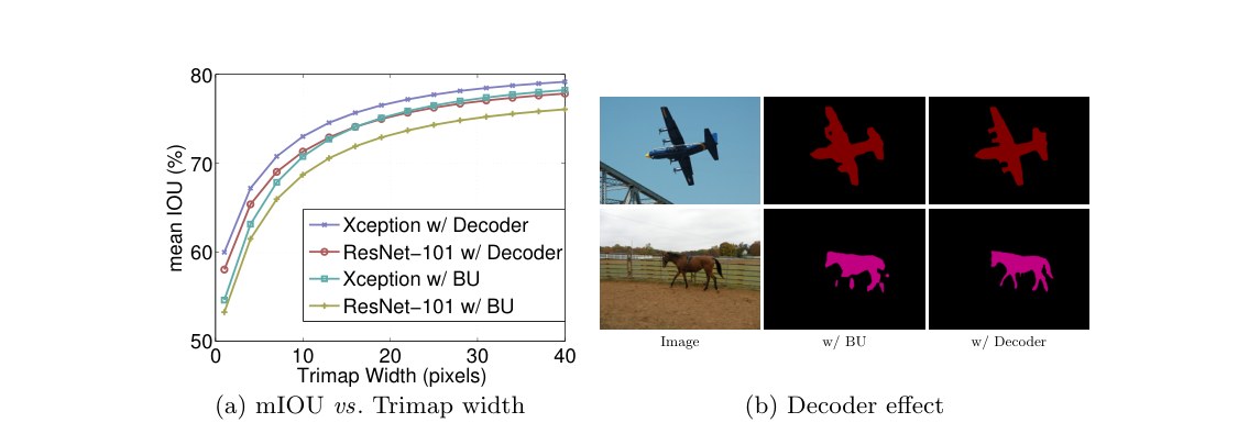
Figure 5: (a) mIOU as a function of trimap band width around the object boundaries when employing . BU: Bilinear upsampling. (b) Qualitative effect of employing the proposed decoder module compared with the naive bilinear upsampling (denoted as BU). In the examples, we adopt Xception as feature extractor and .
图 5:(a)当采用 时,mIOU 作为物体边界周围 trimap 带宽的函数。BU:双线性上采样。(b)采用提出的解码器模块相对朴素双线性上采样(记为 BU)的定性效果。在这些例子中,我们采用 Xception 作为特征抽取器,并且 。
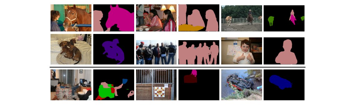
Figure 6: Visualization results on val set. The last row shows a failure mode.
图 6:val 集上的可视化结果。最后一行展示了一种失败模式。
4.5 Experimental Results on Cityscapes
4.5 在 Cityscapes 上的实验结果
In this section, we experiment DeepLabv3+ on the Cityscapes dataset [3], a large-scale dataset containing high quality pixel-level annotations of 5000 images (2975, 500, and 1525 for the training, validation, and test sets respectively) and about 20000 coarsely annotated images.
本节中,我们在 Cityscapes 数据集 [3] 上实验 DeepLabv3+,这是一个大规模数据集,包含 5000 张高质量像素级标注图像(训练、验证和测试集分别为 2975、500 和 1525 张),以及约 20000 张粗标注图像。
As shown in Tab. 7 (a), employing the proposed Xception model as network backbone (denoted as X-65) on top of DeepLabv3 [23], which includes the ASPP module and image-level features [52], attains the performance of 77.33% on the validation set. Adding the proposed decoder module significantly improves the performance to 78.79% (1.46% improvement). We notice that removing the augmented image-level feature improves the performance to 79.14%, showing that in DeepLab model, the image-level features are more effective on the PASCAL VOC 2012 dataset. We also discover that on the Cityscapes dataset, it is effective to increase more layers in the entry flow in the Xception [26], the same as what [31] did for the object detection task. The resulting model building on top of the deeper network backbone (denoted as X-71 in the table), attains the best performance of 79.55% on the validation set.
如表 7 (a) 所示,在包含 ASPP 模块和图像级特征 [52] 的 DeepLabv3 [23] 之上,采用提出的 Xception 模型作为网络主干(记为 X-65),在验证集上达到 77.33% 的性能。加入提出的解码器模块,把性能显著提高到 78.79%(改进 1.46%)。我们注意到,去掉增强的图像级特征会把性能提高到 79.14%,表明在 DeepLab 模型中,图像级特征在 PASCAL VOC 2012 数据集上更为有效。我们还发现,在 Cityscapes 数据集上,增加 Xception [26] 入口流中的层数是有效的,这与 [31] 在物体检测任务上的做法相同。建立在这一更深网络主干(表中记为 X-71)之上的模型,在验证集上达到最好的 79.55% 性能。
After finding the best model variant on val set, we then further fine-tune the model on the coarse annotations in order to compete with other state-of-art models. As shown in Tab. 7 (b), our proposed DeepLabv3+ attains a performance of 82.1% on the test set, setting a new state-of-art performance on Cityscapes.
在 val 集上找到最好的模型变体之后,我们再在粗标注上进一步微调模型,以便与其他当时最好的模型竞争。如表 7 (b) 所示,我们提出的 DeepLabv3+ 在测试集上达到 82.1% 的性能,在 Cityscapes 上树立了新的当时最好水平。
(a) val set results
| Backbone | Decoder | ASPP | Image-Level | mIOU |
|---|---|---|---|---|
| X-65 | ✓ | ✓ | 77.33 | |
| X-65 | ✓ | ✓ | ✓ | 78.79 |
| X-65 | ✓ | ✓ | 79.14 | |
| X-71 | ✓ | ✓ | 79.55 |
(b) test set results
| Method | Coarse | mIOU |
|---|---|---|
| ResNet-38 [83] | ✓ | 80.6 |
| PSPNet [24] | ✓ | 81.2 |
| Mapillary [86] | ✓ | 82.0 |
| DeepLabv3 | ✓ | 81.3 |
| DeepLabv3+ | ✓ | 82.1 |
Table 7: (a) DeepLabv3+ on the Cityscapes val set when trained with train_fine set. (b) DeepLabv3+ on Cityscapes test set. Coarse: Use train_extra set (coarse annotations) as well. Only a few top models are listed in this table.
(a) 验证集结果
| 主干 | 解码器 | ASPP | 图像级 | mIOU |
|---|---|---|---|---|
| X-65 | ✓ | ✓ | 77.33 | |
| X-65 | ✓ | ✓ | ✓ | 78.79 |
| X-65 | ✓ | ✓ | 79.14 | |
| X-71 | ✓ | ✓ | 79.55 |
(b) 测试集结果
| 方法 | 粗标注 | mIOU |
|---|---|---|
| ResNet-38 [83] | ✓ | 80.6 |
| PSPNet [24] | ✓ | 81.2 |
| Mapillary [86] | ✓ | 82.0 |
| DeepLabv3 | ✓ | 81.3 |
| DeepLabv3+ | ✓ | 82.1 |
表 7:(a)用 train_fine 集训练时,DeepLabv3+ 在 Cityscapes val 集上的结果。(b)DeepLabv3+ 在 Cityscapes test 集上的结果。Coarse:同时使用 train_extra 集(粗标注)。本表只列出少数表现最好的模型。
5 Conclusion
5 结论
Our proposed model “DeepLabv3+” employs the encoder-decoder structure where DeepLabv3 is used to encode the rich contextual information and a simple yet effective decoder module is adopted to recover the object boundaries. One could also apply the atrous convolution to extract the encoder features at an arbitrary resolution, depending on the available computation resources. We also explore the Xception model and atrous separable convolution to make the proposed model faster and stronger. Finally, our experimental results show that the proposed model sets a new state-of-the-art performance on PASCAL VOC 2012 and Cityscapes datasets.
我们提出的模型 “DeepLabv3+” 采用编码器–解码器结构,其中 DeepLabv3 被用来编码丰富的上下文信息,一个简单却有效的解码器模块被用来恢复物体边界。人们也可以视可用的计算资源,应用空洞卷积在任意分辨率上抽取编码器特征。我们还探索了 Xception 模型和空洞可分离卷积,以使提出的模型更快、更强。最后,我们的实验结果表明,提出的模型在 PASCAL VOC 2012 和 Cityscapes 数据集上树立了新的当时最好性能。
Acknowledgments We would like to acknowledge the valuable discussions with Haozhi Qi and Jifeng Dai about Aligned Xception, the feedback from Chen Sun, and the support from Google Mobile Vision team.
致谢 我们感谢与 Haozhi Qi 和 Jifeng Dai 就 Aligned Xception 的有益讨论、来自 Chen Sun 的反馈,以及 Google Mobile Vision 团队的支持。
References
参考文献
[1] Everingham, M., Eslami, S.M.A., Gool, L.V., Williams, C.K.I., Winn, J., Zisserman, A.: The pascal visual object classes challenge – a retrospective. IJCV (2014)
[2] Mottaghi, R., Chen, X., Liu, X., Cho, N.G., Lee, S.W., Fidler, S., Urtasun, R., Yuille, A.: The role of context for object detection and semantic segmentation in the wild. In: CVPR. (2014)
[3] Cordts, M., Omran, M., Ramos, S., Rehfeld, T., Enzweiler, M., Benenson, R., Franke, U., Roth, S., Schiele, B.: The cityscapes dataset for semantic urban scene understanding. In: CVPR. (2016)
[4] Zhou, B., Zhao, H., Puig, X., Fidler, S., Barriuso, A., Torralba, A.: Scene parsing through ade20k dataset. In: CVPR. (2017)
[5] Caesar, H., Uijlings, J., Ferrari, V.: COCO-Stuff: Thing and stuff classes in context. In: CVPR. (2018)
[6] LeCun, Y., Bottou, L., Bengio, Y., Haffner, P.: Gradient-based learning applied to document recognition. In: Proc. IEEE. (1998)
[7] Krizhevsky, A., Sutskever, I., Hinton, G.E.: Imagenet classification with deep convolutional neural networks. In: NIPS. (2012)
[8] Sermanet, P., Eigen, D., Zhang, X., Mathieu, M., Fergus, R., LeCun, Y.: Overfeat: Integrated recognition, localization and detection using convolutional networks. In: ICLR. (2014)
[9] Simonyan, K., Zisserman, A.: Very deep convolutional networks for large-scale image recognition. In: ICLR. (2015)
[10] Szegedy, C., Liu, W., Jia, Y., Sermanet, P., Reed, S., Anguelov, D., Erhan, D., Vanhoucke, V., Rabinovich, A.: Going deeper with convolutions. In: CVPR. (2015)
[11] Long, J., Shelhamer, E., Darrell, T.: Fully convolutional networks for semantic segmentation. In: CVPR. (2015)
[12] He, X., Zemel, R.S., Carreira-Perpindn, M.: Multiscale conditional random fields for image labeling. In: CVPR. (2004)
[13] Shotton, J., Winn, J., Rother, C., Criminisi, A.: Textonboost for image understanding: Multi-class object recognition and segmentation by jointly modeling texture, layout, and context. IJCV (2009)
[14] Kohli, P., Torr, P.H., et al.: Robust higher order potentials for enforcing label consistency. IJCV 82 (3) (2009) 302–324
[15] Ladicky, L., Russell, C., Kohli, P., Torr, P.H.: Associative hierarchical crfs for object class image segmentation. In: ICCV. (2009)
[16] Gould, S., Fulton, R., Koller, D.: Decomposing a scene into geometric and semantically consistent regions. In: ICCV. (2009)
[17] Yao, J., Fidler, S., Urtasun, R.: Describing the scene as a whole: Joint object detection, scene classification and semantic segmentation. In: CVPR. (2012)
[18] Grauman, K., Darrell, T.: The pyramid match kernel: Discriminative classification with sets of image features. In: ICCV. (2005)
[19] Lazebnik, S., Schmid, C., Ponce, J.: Beyond bags of features: Spatial pyramid matching for recognizing natural scene categories. In: CVPR. (2006)
[20] He, K., Zhang, X., Ren, S., Sun, J.: Spatial pyramid pooling in deep convolutional networks for visual recognition. In: ECCV. (2014)
[21] Ronneberger, O., Fischer, P., Brox, T.: U-net: Convolutional networks for biomedical image segmentation. In: MICCAI. (2015)
[22] Badrinarayanan, V., Kendall, A., Cipolla, R.: Segnet: A deep convolutional encoder-decoder architecture for image segmentation. PAMI (2017)
[23] Chen, L.C., Papandreou, G., Schroff, F., Adam, H.: Rethinking atrous convolution for semantic image segmentation. arXiv:1706.05587 (2017)
[24] Zhao, H., Shi, J., Qi, X., Wang, X., Jia, J.: Pyramid scene parsing network. In: CVPR. (2017)
[25] He, K., Zhang, X., Ren, S., Sun, J.: Deep residual learning for image recognition. In: CVPR. (2016)
[26] Chollet, F.: Xception: Deep learning with depthwise separable convolutions. In: CVPR. (2017)
[27] Sifre, L.: Rigid-motion scattering for image classification. PhD thesis (2014)
[28] Vanhoucke, V.: Learning visual representations at scale. ICLR invited talk (2014)
[29] Howard, A.G., Zhu, M., Chen, B., Kalenichenko, D., Wang, W., Weyand, T., Andreetto, M., Adam, H.: Mobilenets: Efficient convolutional neural networks for mobile vision applications. arXiv:1704.04861 (2017)
[30] Zhang, X., Zhou, X., Lin, M., Sun, J.: Shufflenet: An extremely efficient convolutional neural network for mobile devices. In: CVPR. (2018)
[31] Qi, H., Zhang, Z., Xiao, B., Hu, H., Cheng, B., Wei, Y., Dai, J.: Deformable convolutional networks – coco detection and segmentation challenge 2017 entry. ICCV COCO Challenge Workshop (2017)
[32] Mostajabi, M., Yadollahpour, P., Shakhnarovich, G.: Feedforward semantic segmentation with zoom-out features. In: CVPR. (2015)
[33] Dai, J., He, K., Sun, J.: Convolutional feature masking for joint object and stuff segmentation. In: CVPR. (2015)
[34] Farabet, C., Couprie, C., Najman, L., LeCun, Y.: Learning hierarchical features for scene labeling. PAMI (2013)
[35] Eigen, D., Fergus, R.: Predicting depth, surface normals and semantic labels with a common multi-scale convolutional architecture. In: ICCV. (2015)
[36] Pinheiro, P., Collobert, R.: Recurrent convolutional neural networks for scene labeling. In: ICML. (2014)
[37] Lin, G., Shen, C., van den Hengel, A., Reid, I.: Efficient piecewise training of deep structured models for semantic segmentation. In: CVPR. (2016)
[38] Chen, L.C., Yang, Y., Wang, J., Xu, W., Yuille, A.L.: Attention to scale: Scale-aware semantic image segmentation. In: CVPR. (2016)
[39] Chen, L.C., Papandreou, G., Kokkinos, I., Murphy, K., Yuille, A.L.: Deeplab: Semantic image segmentation with deep convolutional nets, atrous convolution, and fully connected crfs. TPAMI (2017)
[40] Krähenbühl, P., Koltun, V.: Efficient inference in fully connected crfs with gaussian edge potentials. In: NIPS. (2011)
[41] Adams, A., Baek, J., Davis, M.A.: Fast high-dimensional filtering using the permutohedral lattice. In: Eurographics. (2010)
[42] Chen, L.C., Papandreou, G., Kokkinos, I., Murphy, K., Yuille, A.L.: Semantic image segmentation with deep convolutional nets and fully connected crfs. In: ICLR. (2015)
[43] Bell, S., Upchurch, P., Snavely, N., Bala, K.: Material recognition in the wild with the materials in context database. In: CVPR. (2015)
[44] Zheng, S., Jayasumana, S., Romera-Paredes, B., Vineet, V., Su, Z., Du, D., Huang, C., Torr, P.: Conditional random fields as recurrent neural networks. In: ICCV. (2015)
[45] Liu, Z., Li, X., Luo, P., Loy, C.C., Tang, X.: Semantic image segmentation via deep parsing network. In: ICCV. (2015)
[46] Papandreou, G., Chen, L.C., Murphy, K., Yuille, A.L.: Weakly- and semi-supervised learning of a dcnn for semantic image segmentation. In: ICCV. (2015)
[47] Schwing, A.G., Urtasun, R.: Fully connected deep structured networks. arXiv:1503.02351 (2015)
[48] Jampani, V., Kiefel, M., Gehler, P.V.: Learning sparse high dimensional filters: Image filtering, dense crfs and bilateral neural networks. In: CVPR. (2016)
[49] Vemulapalli, R., Tuzel, O., Liu, M.Y., Chellappa, R.: Gaussian conditional random field network for semantic segmentation. In: CVPR. (2016)
[50] Chandra, S., Kokkinos, I.: Fast, exact and multi-scale inference for semantic image segmentation with deep Gaussian CRFs. In: ECCV. (2016)
[51] Chandra, S., Usunier, N., Kokkinos, I.: Dense and low-rank gaussian crfs using deep embeddings. In: ICCV. (2017)
[52] Liu, W., Rabinovich, A., Berg, A.C.: Parsenet: Looking wider to see better. arXiv:1506.04579 (2015)
[53] Newell, A., Yang, K., Deng, J.: Stacked hourglass networks for human pose estimation. In: ECCV. (2016)
[54] Lin, T.Y., Dollár, P., Girshick, R., He, K., Hariharan, B., Belongie, S.: Feature pyramid networks for object detection. In: CVPR. (2017)
[55] Shrivastava, A., Sukthankar, R., Malik, J., Gupta, A.: Beyond skip connections: Top-down modulation for object detection. arXiv:1612.06851 (2016)
[56] Fu, C.Y., Liu, W., Ranga, A., Tyagi, A., Berg, A.C.: Dssd: Deconvolutional single shot detector. arXiv:1701.06659 (2017)
[57] Noh, H., Hong, S., Han, B.: Learning deconvolution network for semantic segmentation. In: ICCV. (2015)
[58] Lin, G., Milan, A., Shen, C., Reid, I.: Refinenet: Multi-path refinement networks with identity mappings for high-resolution semantic segmentation. In: CVPR. (2017)
[59] Pohlen, T., Hermans, A., Mathias, M., Leibe, B.: Full-resolution residual networks for semantic segmentation in street scenes. In: CVPR. (2017)
[60] Peng, C., Zhang, X., Yu, G., Luo, G., Sun, J.: Large kernel matters–improve semantic segmentation by global convolutional network. In: CVPR. (2017)
[61] Islam, M.A., Rochan, M., Bruce, N.D., Wang, Y.: Gated feedback refinement network for dense image labeling. In: CVPR. (2017)
[62] Wojna, Z., Ferrari, V., Guadarrama, S., Silberman, N., Chen, L.C., Fathi, A., Uijlings, J.: The devil is in the decoder. In: BMVC. (2017)
[63] Fu, J., Liu, J., Wang, Y., Lu, H.: Stacked deconvolutional network for semantic segmentation. arXiv:1708.04943 (2017)
[64] Zhang, Z., Zhang, X., Peng, C., Cheng, D., Sun, J.: Exfuse: Enhancing feature fusion for semantic segmentation. In: ECCV. (2018)
[65] Xie, S., Girshick, R., Dollár, P., Tu, Z., He, K.: Aggregated residual transformations for deep neural networks. In: CVPR. (2017)
[66] Jin, J., Dundar, A., Culurciello, E.: Flattened convolutional neural networks for feedforward acceleration. arXiv:1412.5474 (2014)
[67] Wang, M., Liu, B., Foroosh, H.: Design of efficient convolutional layers using single intra-channel convolution, topological subdivisioning and spatial ”bottleneck” structure. arXiv:1608.04337 (2016)
[68] Zoph, B., Vasudevan, V., Shlens, J., Le, Q.V.: Learning transferable architectures for scalable image recognition. In: CVPR. (2018)
[69] Holschneider, M., Kronland-Martinet, R., Morlet, J., Tchamitchian, P.: A real-time algorithm for signal analysis with the help of the wavelet transform. In: Wavelets: Time-Frequency Methods and Phase Space. (1989) 289–297
[70] Giusti, A., Ciresan, D., Masci, J., Gambardella, L., Schmidhuber, J.: Fast image scanning with deep max-pooling convolutional neural networks. In: ICIP. (2013)
[71] Papandreou, G., Kokkinos, I., Savalle, P.A.: Modeling local and global deformations in deep learning: Epitomic convolution, multiple instance learning, and sliding window detection. In: CVPR. (2015)
[72] Abadi, M., Agarwal, A., et al.: Tensorflow: Large-scale machine learning on heterogeneous distributed systems. arXiv:1603.04467 (2016)
[73] Hariharan, B., Arbeláez, P., Girshick, R., Malik, J.: Hypercolumns for object segmentation and fine-grained localization. In: CVPR. (2015)
[74] Russakovsky, O., Deng, J., Su, H., Krause, J., Satheesh, S., Ma, S., Huang, Z., Karpathy, A., Khosla, A., Bernstein, M., Berg, A.C., Fei-Fei, L.: ImageNet Large Scale Visual Recognition Challenge. IJCV (2015)
[75] Ioffe, S., Szegedy, C.: Batch normalization: Accelerating deep network training by reducing internal covariate shift. In: ICML. (2015)
[76] Hariharan, B., Arbeláez, P., Bourdev, L., Maji, S., Malik, J.: Semantic contours from inverse detectors. In: ICCV. (2011)
[77] Wang, P., Chen, P., Yuan, Y., Liu, D., Huang, Z., Hou, X., Cottrell, G.: Understanding convolution for semantic segmentation. arXiv:1702.08502 (2017)
[78] Dai, J., Qi, H., Xiong, Y., Li, Y., Zhang, G., Hu, H., Wei, Y.: Deformable convolutional networks. In: ICCV. (2017)
[79] Lin, T.Y., et al.: Microsoft COCO: Common objects in context. In: ECCV. (2014)
[80] Hinton, G., Vinyals, O., Dean, J.: Distilling the knowledge in a neural network. In: NIPS. (2014)
[81] Sun, C., Shrivastava, A., Singh, S., Gupta, A.: Revisiting unreasonable effectiveness of data in deep learning era. In: ICCV. (2017)
[82] Li, X., Liu, Z., Luo, P., Loy, C.C., Tang, X.: Not all pixels are equal: Difficulty-aware semantic segmentation via deep layer cascade. In: CVPR. (2017)
[83] Wu, Z., Shen, C., van den Hengel, A.: Wider or deeper: Revisiting the resnet model for visual recognition. arXiv:1611.10080 (2016)
[84] Wang, G., Luo, P., Lin, L., Wang, X.: Learning object interactions and descriptions for semantic image segmentation. In: CVPR. (2017)
[85] Luo, P., Wang, G., Lin, L., Wang, X.: Deep dual learning for semantic image segmentation. In: ICCV. (2017)
[86] Bulò, S.R., Porzi, L., Kontschieder, P.: In-place activated batchnorm for memory-optimized training of dnns. In: CVPR. (2018)