DeepLab: Semantic Image Segmentation with Deep Convolutional Nets, Atrous Convolution, and Fully Connected CRFs

DeepLab：深度卷积网络、空洞卷积与全连接 CRF 的语义图像分割

Liang-Chieh Chen    George Papandreou    Iasonas Kokkinos    Kevin Murphy    Alan L. Yuille † † thanks: L.-C. Chen, G. Papandreou, and K. Murphy are with Google Inc. I. Kokkinos is with University College London. A. Yuille is with the Departments of Cognitive Science and Computer Science, Johns Hopkins University. The first two authors contributed equally to this work.

Abstract

摘要

In this work we address the task of semantic image segmentation with Deep Learning and make three main contributions that are experimentally shown to have substantial practical merit. First, we highlight convolution with upsampled filters, or ‘atrous convolution’, as a powerful tool in dense prediction tasks. Atrous convolution allows us to explicitly control the resolution at which feature responses are computed within Deep Convolutional Neural Networks. It also allows us to effectively enlarge the field of view of filters to incorporate larger context without increasing the number of parameters or the amount of computation. Second, we propose atrous spatial pyramid pooling (ASPP) to robustly segment objects at multiple scales. ASPP probes an incoming convolutional feature layer with filters at multiple sampling rates and effective fields-of-views, thus capturing objects as well as image context at multiple scales. Third, we improve the localization of object boundaries by combining methods from DCNNs and probabilistic graphical models. The commonly deployed combination of max-pooling and downsampling in DCNNs achieves invariance but has a toll on localization accuracy. We overcome this by combining the responses at the final DCNN layer with a fully connected Conditional Random Field (CRF), which is shown both qualitatively and quantitatively to improve localization performance. Our proposed “DeepLab” system sets the new state-of-art at the PASCAL VOC-2012 semantic image segmentation task, reaching 79.7% mIOU in the test set, and advances the results on three other datasets: PASCAL-Context, PASCAL-Person-Part, and Cityscapes. All of our code is made publicly available online.

本文用深度学习做语义图像分割，提出三点经实验证明很有实用价值的贡献。第一，我们强调用上采样滤波器做卷积，即「空洞卷积」（atrous convolution），作为稠密预测任务里的有力工具。空洞卷积能显式控制深度卷积网络里特征响应的计算分辨率，也能在不增加参数量和计算量的前提下有效扩大滤波器感受野，纳入更大范围上下文。第二，我们提出空洞空间金字塔池化（ASPP），在多尺度上稳健地分割物体。ASPP 用多种采样率、多种有效感受野的滤波器探测同一卷积特征层，从而同时捕获多尺度物体与图像上下文。第三，我们把 DCNN 与概率图模型结合起来，改善物体边界定位。DCNN 里常用的最大池化与下采样组合带来不变性，却牺牲定位精度；我们把最终 DCNN 层的响应与全连接条件随机场（CRF）结合，定性和定量都显示边界定位更好。所提出的「DeepLab」系统在 PASCAL VOC-2012 语义分割任务上刷新当时最优，测试集达到 79.7% mIOU，并在 PASCAL-Context、PASCAL-Person-Part 与 Cityscapes 三个数据集上推进结果。全部代码已公开。

I Introduction

I 引言

Index Terms:

Deep Convolutional Neural Networks (DCNNs) [1] have pushed the performance of computer vision systems to soaring heights on a broad array of high-level problems, including image classification [2, 3, 4, 5, 6] and object detection [7, 8, 9, 10, 11, 12], where DCNNs trained in an end-to-end manner have delivered strikingly better results than systems relying on hand-crafted features. Essential to this success is the built-in invariance of DCNNs to local image transformations, which allows them to learn increasingly abstract data representations [13]. This invariance is clearly desirable for classification tasks, but can hamper dense prediction tasks such as semantic segmentation, where abstraction of spatial information is undesired.

索引词：

深度卷积网络（DCNN）[1] 把计算机视觉在图像分类 [2, 3, 4, 5, 6]、目标检测 [7, 8, 9, 10, 11, 12] 等高层任务上的表现推到很高的水平：端到端训练的 DCNN 明显好于依赖手工特征的系统。成功的关键在于 DCNN 对局部图像变换的内置不变性，使网络能学到越来越抽象的表示 [13]。分类任务显然需要这种不变性，但对语义分割这类稠密预测任务，空间信息被过度抽象反而不利。

In particular we consider three challenges in the application of DCNNs to semantic image segmentation: (1) reduced feature resolution, (2) existence of objects at multiple scales, and (3) reduced localization accuracy due to DCNN invariance. Next, we discuss these challenges and our approach to overcome them in our proposed DeepLab system.

具体来说，把 DCNN 用到语义图像分割时，我们关注三个难点：（1）特征分辨率下降；（2）物体尺度多样；（3）DCNN 不变性导致定位精度下降。下文讨论这些难点，以及我们在 DeepLab 中的应对。

The first challenge is caused by the repeated combination of max-pooling and downsampling (‘striding’) performed at consecutive layers of DCNNs originally designed for image classification [2, 4, 5]. This results in feature maps with significantly reduced spatial resolution when the DCNN is employed in a fully convolutional fashion [14]. In order to overcome this hurdle and efficiently produce denser feature maps, we remove the downsampling operator from the last few max pooling layers of DCNNs and instead upsample the filters in subsequent convolutional layers, resulting in feature maps computed at a higher sampling rate. Filter upsampling amounts to inserting holes (‘trous’ in French) between nonzero filter taps. This technique has a long history in signal processing, originally developed for the efficient computation of the undecimated wavelet transform in a scheme also known as “algorithme à trous” [15]. We use the term atrous convolution as a shorthand for convolution with upsampled filters. Various flavors of this idea have been used before in the context of DCNNs by [16, 3, 6]. In practice, we recover full resolution feature maps by a combination of atrous convolution, which computes feature maps more densely, followed by simple bilinear interpolation of the feature responses to the original image size. This scheme offers a simple yet powerful alternative to using deconvolutional layers [13, 14] in dense prediction tasks. Compared to regular convolution with larger filters, atrous convolution allows us to effectively enlarge the field of view of filters without increasing the number of parameters or the amount of computation.

第一个难点来自原先为图像分类设计的 DCNN [2, 4, 5]：连续层反复做最大池化与下采样（stride），以全卷积方式使用时特征图空间分辨率会大幅下降 [14]。为高效得到更稠密的特征图，我们去掉末尾若干最大池化层的下采样，并在后续卷积层中上采样滤波器，从而以更高采样率计算特征图。滤波器上采样相当于在非零抽头之间插入空洞（法语「trous」）。该技术在信号处理中历史很长，最初用于高效计算非抽取小波变换，也称作「algorithme à trous」[15]。我们把带上采样滤波器的卷积简称为空洞卷积。DCNN 语境下 [16, 3, 6] 也曾用过多种变体。实践中，我们先用空洞卷积更稠密地算特征图，再用简单双线性插值把响应拉回原图尺寸，从而恢复全分辨率特征图。这为稠密预测任务提供了相对反卷积层 [13, 14] 更简单有力的替代。与更大核的常规卷积相比，空洞卷积能在不增加参数与计算的前提下有效扩大感受野。

The second challenge is caused by the existence of objects at multiple scales. A standard way to deal with this is to present to the DCNN rescaled versions of the same image and then aggregate the feature or score maps [6, 17, 18]. We show that this approach indeed increases the performance of our system, but comes at the cost of computing feature responses at all DCNN layers for multiple scaled versions of the input image. Instead, motivated by spatial pyramid pooling [19, 20], we propose a computationally efficient scheme of resampling a given feature layer at multiple rates prior to convolution. This amounts to probing the original image with multiple filters that have complementary effective fields of view, thus capturing objects as well as useful image context at multiple scales. Rather than actually resampling features, we efficiently implement this mapping using multiple parallel atrous convolutional layers with different sampling rates; we call the proposed technique “atrous spatial pyramid pooling” (ASPP).

第二个难点来自物体多尺度。常见做法是把同一图像的多种缩放版本送入 DCNN，再聚合特征或分数图 [6, 17, 18]。我们证明这确实能提升系统表现，但代价是要对多种尺度的输入在所有 DCNN 层上算特征响应。受空间金字塔池化启发 [19, 20]，我们提出一种计算更省的方案：在卷积前对给定特征层按多种采样率重采样。这相当于用互补有效感受野的多组滤波器探测原图，从而在多尺度上捕获物体与有用上下文。我们并不真正重采样特征，而是用不同采样率的多路并行空洞卷积高效实现；我们称该技术为「空洞空间金字塔池化」（ASPP）。

The third challenge relates to the fact that an object-centric classifier requires invariance to spatial transformations, inherently limiting the spatial accuracy of a DCNN. One way to mitigate this problem is to use skip-layers to extract “hyper-column” features from multiple network layers when computing the final segmentation result [21, 14]. Our work explores an alternative approach which we show to be highly effective. In particular, we boost our model’s ability to capture fine details by employing a fully-connected Conditional Random Field (CRF) [22]. CRFs have been broadly used in semantic segmentation to combine class scores computed by multi-way classifiers with the low-level information captured by the local interactions of pixels and edges [23, 24] or superpixels [25]. Even though works of increased sophistication have been proposed to model the hierarchical dependency [26, 27, 28] and/or high-order dependencies of segments [29, 30, 31, 32, 33], we use the fully connected pairwise CRF proposed by [22] for its efficient computation, and ability to capture fine edge details while also catering for long range dependencies. That model was shown in [22] to improve the performance of a boosting-based pixel-level classifier. In this work, we demonstrate that it leads to state-of-the-art results when coupled with a DCNN-based pixel-level classifier.

第三个难点在于：以物体为中心的分类器需要空间变换不变性，这天然限制了 DCNN 的空间精度。一种缓解办法是用跳跃连接，在最终分割时从多层抽取「超列」特征 [21, 14]。本文探索另一条被证明很有效的路线：用全连接条件随机场（CRF）[22] 增强模型捕获细粒度细节的能力。语义分割里 CRF 被广泛用来把多类分类器的类别分数与像素、边缘 [23, 24] 或超像素 [25] 的局部交互所携带的低层信息结合起来。尽管已有更复杂的工作建模层次依赖 [26, 27, 28] 和/或片段高阶依赖 [29, 30, 31, 32, 33]，我们采用 [22] 的全连接成对 CRF，因其计算高效，既能抓住细边缘细节，又能照顾长程依赖。[22] 已证明该模型能提升基于 Boosting 的像素级分类器；本文则证明它与基于 DCNN 的像素级分类器结合也能达到当时最优。

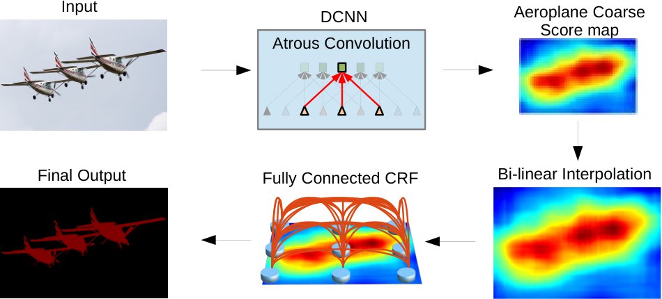
Fig. 1: Model Illustration. A Deep Convolutional Neural Network such as VGG-16 or ResNet-101 is employed in a fully convolutional fashion, using atrous convolution to reduce the degree of signal downsampling (from 32x down 8x). A bilinear interpolation stage enlarges the feature maps to the original image resolution. A fully connected CRF is then applied to refine the segmentation result and better capture the object boundaries.

图 1：模型示意。以全卷积方式使用 VGG-16 或 ResNet-101 等深度卷积网络，并用空洞卷积降低信号下采样程度（从 32 倍降到 8 倍）。双线性插值阶段把特征图放大到原图分辨率，再施加全连接 CRF 细化分割结果、更好抓住物体边界。

A high-level illustration of the proposed DeepLab model is shown in Fig. 1. A deep convolutional neural network (VGG-16 [4] or ResNet-101 [11] in this work) trained in the task of image classification is re-purposed to the task of semantic segmentation by (1) transforming all the fully connected layers to convolutional layers (i.e., fully convolutional network [14]) and (2) increasing feature resolution through atrous convolutional layers, allowing us to compute feature responses every 8 pixels instead of every 32 pixels in the original network. We then employ bi-linear interpolation to upsample by a factor of 8 the score map to reach the original image resolution, yielding the input to a fully-connected CRF [22] that refines the segmentation results.

所提 DeepLab 模型的高层示意见图 1。在图像分类任务上训练好的深度卷积网络（本文用 VGG-16 [4] 或 ResNet-101 [11]）被改用于语义分割：（1）把所有全连接层改成卷积层（即全卷积网络 [14]）；（2）通过空洞卷积提高特征分辨率，使特征响应每隔 8 个像素计算一次，而不是原网络中的每隔 32 个像素。再用双线性插值把分数图上采样 8 倍到原图分辨率，作为全连接 CRF [22] 的输入以细化分割。

From a practical standpoint, the three main advantages of our DeepLab system are: (1) Speed: by virtue of atrous convolution, our dense DCNN operates at 8 FPS on an NVidia Titan X GPU, while Mean Field Inference for the fully-connected CRF requires 0.5 secs on a CPU. (2) Accuracy: we obtain state-of-art results on several challenging datasets, including the PASCAL VOC 2012 semantic segmentation benchmark [34], PASCAL-Context [35], PASCAL-Person-Part [36], and Cityscapes [37]. (3) Simplicity: our system is composed of a cascade of two very well-established modules, DCNNs and CRFs.

从实用角度看，DeepLab 系统有三大优势：（1）速度：借助空洞卷积，稠密 DCNN 在 NVidia Titan X GPU 上约 8 FPS，全连接 CRF 的均值场推断在 CPU 上约需 0.5 秒。（2）精度：在多个挑战性数据集上达到当时最优，包括 PASCAL VOC 2012 语义分割基准 [34]、PASCAL-Context [35]、PASCAL-Person-Part [36] 与 Cityscapes [37]。（3）简洁：系统由 DCNN 与 CRF 两个非常成熟的模块级联而成。

The updated DeepLab system we present in this paper features several improvements compared to its first version reported in our original conference publication [38]. Our new version can better segment objects at multiple scales, via either multi-scale input processing [39, 40, 17] or the proposed ASPP. We have built a residual net variant of DeepLab by adapting the state-of-art ResNet [11] image classification DCNN, achieving better semantic segmentation performance compared to our original model based on VGG-16 [4]. Finally, we present a more comprehensive experimental evaluation of multiple model variants and report state-of-art results not only on the PASCAL VOC 2012 benchmark but also on other challenging tasks. We have implemented the proposed methods by extending the Caffe framework [41]. We share our code and models at a companion web site http://liangchiehchen.com/projects/DeepLab.html.

相对会议版首次报告 [38]，本文更新的 DeepLab 有若干改进。新版本能更好分割多尺度物体，途径包括多尺度输入处理 [39, 40, 17] 或所提 ASPP。我们把当时最优的 ResNet [11] 图像分类 DCNN 改造成 DeepLab 的残差网络变体，语义分割表现优于原先基于 VGG-16 [4] 的模型。最后，我们对多种模型变体做了更全面实验评估，不仅在 PASCAL VOC 2012 基准、也在其他挑战任务上报告当时最优结果。方法通过扩展 Caffe 框架 [41] 实现。代码与模型见配套网站 http://liangchiehchen.com/projects/DeepLab.html。

II Related Work

II 相关工作

Most of the successful semantic segmentation systems developed in the previous decade relied on hand-crafted features combined with flat classifiers, such as Boosting [42, 24], Random Forests [43], or Support Vector Machines [44]. Substantial improvements have been achieved by incorporating richer information from context [45] and structured prediction techniques [26, 27, 46, 22], but the performance of these systems has always been compromised by the limited expressive power of the features. Over the past few years the breakthroughs of Deep Learning in image classification were quickly transferred to the semantic segmentation task. Since this task involves both segmentation and classification, a central question is how to combine the two tasks.

过去十年多数成功的语义分割系统依赖手工特征，再配合 Boosting [42, 24]、随机森林 [43] 或支持向量机 [44] 等扁平分类器。引入更丰富的上下文 [45] 与结构化预测技术 [26, 27, 46, 22] 带来了明显提升，但特征表达能力有限始终制约上限。近年来深度学习在图像分类上的突破很快迁移到语义分割。该任务同时涉及分割与分类，核心问题是如何把二者结合起来。

The first family of DCNN-based systems for semantic segmentation typically employs a cascade of bottom-up image segmentation, followed by DCNN-based region classification. For instance the bounding box proposals and masked regions delivered by [47, 48] are used in [7] and [49] as inputs to a DCNN to incorporate shape information into the classification process. Similarly, the authors of [50] rely on a superpixel representation. Even though these approaches can benefit from the sharp boundaries delivered by a good segmentation, they also cannot recover from any of its errors.

第一类基于 DCNN 的语义分割系统通常做自底向上图像分割，再接 DCNN 区域分类。[47, 48] 给出的边界框提议与掩膜区域被 [7] 与 [49] 用作 DCNN 输入，以把形状信息纳入分类。[50] 则依赖超像素表示。这类方法能受益于好分割给出的锐利边界，但一旦分割出错便难以挽回。

The second family of works relies on using convolutionally computed DCNN features for dense image labeling, and couples them with segmentations that are obtained independently. Among the first have been [39] who apply DCNNs at multiple image resolutions and then employ a segmentation tree to smooth the prediction results. More recently, [21] propose to use skip layers and concatenate the computed intermediate feature maps within the DCNNs for pixel classification. Further, [51] propose to pool the intermediate feature maps by region proposals. These works still employ segmentation algorithms that are decoupled from the DCNN classifier’s results, thus risking commitment to premature decisions.

第二类工作用卷积算出的 DCNN 特征做稠密图像标注，再与独立得到的分割结果耦合。较早的 [39] 在多种图像分辨率上跑 DCNN，再用分割树平滑预测。更近的 [21] 提出用跳跃层，拼接 DCNN 中间特征图做像素分类。[51] 则按区域提议对中间特征图做池化。这些工作仍使用与 DCNN 分类结果解耦的分割算法，可能过早固定错误决策。

The third family of works uses DCNNs to directly provide dense category-level pixel labels, which makes it possible to even discard segmentation altogether. The segmentation-free approaches of [14, 52] directly apply DCNNs to the whole image in a fully convolutional fashion, transforming the last fully connected layers of the DCNN into convolutional layers. In order to deal with the spatial localization issues outlined in the introduction, [14] upsample and concatenate the scores from intermediate feature maps, while [52] refine the prediction result from coarse to fine by propagating the coarse results to another DCNN. Our work builds on these works, and as described in the introduction extends them by exerting control on the feature resolution, introducing multi-scale pooling techniques and integrating the densely connected CRF of [22] on top of the DCNN. We show that this leads to significantly better segmentation results, especially along object boundaries. The combination of DCNN and CRF is of course not new but previous works only tried locally connected CRF models. Specifically, [53] use CRFs as a proposal mechanism for a DCNN-based reranking system, while [39] treat superpixels as nodes for a local pairwise CRF and use graph-cuts for discrete inference. As such their models were limited by errors in superpixel computations or ignored long-range dependencies. Our approach instead treats every pixel as a CRF node receiving unary potentials by the DCNN. Crucially, the Gaussian CRF potentials in the fully connected CRF model of [22] that we adopt can capture long-range dependencies and at the same time the model is amenable to fast mean field inference. We note that mean field inference had been extensively studied for traditional image segmentation tasks [54, 55, 56], but these older models were typically limited to short-range connections. In independent work, [57] use a very similar densely connected CRF model to refine the results of DCNN for the problem of material classification. However, the DCNN module of [57] was only trained by sparse point supervision instead of dense supervision at every pixel.

第三类工作让 DCNN 直接给出稠密类别级像素标签，甚至可以完全不要分割。[14, 52] 的无分割方法以全卷积方式把 DCNN 直接作用整图，把末尾全连接层改成卷积层。为应对引言所述的空间定位问题，[14] 上采样并拼接中间特征图的分数，[52] 则把粗预测传到另一 DCNN，由粗到细细化。本文建立在这些工作之上，并如引言所述加以扩展：控制特征分辨率、引入多尺度池化，并在 DCNN 之上接入 [22] 的稠密连接 CRF。我们证明这能显著提升分割结果，尤其是物体边界处。DCNN 与 CRF 的组合并非全新，但先前工作多用局部连接 CRF：[53] 把 CRF 当 DCNN 重排序系统的提议机制，[39] 把超像素当局部成对 CRF 的节点并用图割做离散推断。因而其模型受超像素误差限制，或忽略长程依赖。我们的方法把每个像素当作接收 DCNN 一元势的 CRF 节点。关键是，我们采用的 [22] 全连接 CRF 中的高斯势既能捕获长程依赖，又适合快速均值场推断。均值场推断在传统图像分割中已有大量研究 [54, 55, 56]，但那些较早模型通常限于短程连接。独立工作 [57] 用非常相似的稠密连接 CRF 细化材料分类中的 DCNN 结果；不过 [57] 的 DCNN 模块仅用稀疏点监督训练，而非每个像素的稠密监督。

Since the first version of this work was made publicly available [38], the area of semantic segmentation has progressed drastically. Multiple groups have made important advances, significantly raising the bar on the PASCAL VOC 2012 semantic segmentation benchmark, as reflected to the high level of activity in the benchmark’s leaderboard[^1] [58, 59, 60, 61, 62, 40, 17, 63]. Interestingly, most top-performing methods have adopted one or both of the key ingredients of our DeepLab system: Atrous convolution for efficient dense feature extraction and refinement of the raw DCNN scores by means of a fully connected CRF. We outline below some of the most important and interesting advances.

自本工作第一版公开 [38] 以来，语义分割领域进展迅猛。多个团队取得重要突破，显著抬高了 PASCAL VOC 2012 语义分割基准的水准，排行榜活跃度很高[^1] [58, 59, 60, 61, 62, 40, 17, 63]。有意思的是，多数顶尖方法都采纳了 DeepLab 系统的一个或两个关键成分：用空洞卷积做高效稠密特征抽取，以及用全连接 CRF 细化原始 DCNN 分数。下文概述若干最重要、最有意思的进展。

End-to-end training for structured prediction has more recently been explored in several related works. While we employ the CRF as a post-processing method, [59, 64, 65, 62, 40] have successfully pursued joint learning of the DCNN and CRF. In particular, [59, 65] unroll the CRF mean-field inference steps to convert the whole system into an end-to-end trainable feed-forward network, while [62] approximates one iteration of the dense CRF mean field inference [22] by convolutional layers with learnable filters. Another fruitful direction pursued by [40, 66] is to learn the pairwise terms of a CRF via a DCNN, significantly improving performance at the cost of heavier computation. In a different direction, [63] replace the bilateral filtering module used in mean field inference with a faster domain transform module [67], improving the speed and lowering the memory requirements of the overall system, while [68, 18] combine semantic segmentation with edge detection.

结构化预测的端到端训练 近来在若干相关工作中被探索。我们把 CRF 当后处理，而 [59, 64, 65, 62, 40] 成功追求 DCNN 与 CRF 的联合学习。具体地，[59, 65] 展开 CRF 均值场推断步，把整系统变成可端到端训练的前馈网络；[62] 用可学习滤波器的卷积层近似稠密 CRF 均值场推断的一轮 [22]。另一富有成果的方向是 [40, 66]：用 DCNN 学习 CRF 的成对项，显著提升表现但计算更重。另一方向上，[63] 用更快的域变换模块 [67] 替换均值场推断中的双边滤波，提高速度并降低内存；[68, 18] 则把语义分割与边缘检测结合。

Weaker supervision has been pursued in a number of papers, relaxing the assumption that pixel-level semantic annotations are available for the whole training set [69, 58, 70, 71], achieving significantly better results than weakly-supervised pre-DCNN systems such as [72]. In another line of research, [49, 73] pursue instance segmentation, jointly tackling object detection and semantic segmentation.

更弱监督 也在多篇论文中推进，放松了「整个训练集都有像素级语义标注」的假设 [69, 58, 70, 71]，结果明显好于 [72] 等前 DCNN 弱监督系统。另一条线上，[49, 73] 做实例分割，同时处理目标检测与语义分割。

What we call here atrous convolution was originally developed for the efficient computation of the undecimated wavelet transform in the “algorithme à trous” scheme of [15]. We refer the interested reader to [74] for early references from the wavelet literature. Atrous convolution is also intimately related to the “noble identities” in multi-rate signal processing, which builds on the same interplay of input signal and filter sampling rates [75]. Atrous convolution is a term we first used in [6]. The same operation was later called dilated convolution by [76], a term they coined motivated by the fact that the operation corresponds to regular convolution with upsampled (or dilated in the terminology of [15]) filters. Various authors have used the same operation before for denser feature extraction in DCNNs [16, 3, 6]. Beyond mere resolution enhancement, atrous convolution allows us to enlarge the field of view of filters to incorporate larger context, which we have shown in [38] to be beneficial. This approach has been pursued further by [76], who employ a series of atrous convolutional layers with increasing rates to aggregate multiscale context. The atrous spatial pyramid pooling scheme proposed here to capture multiscale objects and context also employs multiple atrous convolutional layers with different sampling rates, which we however lay out in parallel instead of in serial. Interestingly, the atrous convolution technique has also been adopted for a broader set of tasks, such as object detection [12, 77], instance-level segmentation [78], visual question answering [79], and optical flow [80].

我们所说的空洞卷积，最初是为在 [15] 的「algorithme à trous」方案中高效计算非抽取小波变换而发展的。早期小波文献见 [74]。空洞卷积也与多速率信号处理中的「noble identities」密切相关，同样建立在输入信号与滤波器采样率的交互之上 [75]。「atrous convolution」一词我们最先在 [6] 使用；同一操作后来被 [76] 称作 dilated convolution，其动机是该操作对应于用上采样（或按 [15] 术语 dilated）滤波器做常规卷积。此前多位作者已用同一操作在 DCNN 中做更稠密的特征抽取 [16, 3, 6]。除提高分辨率外，空洞卷积还能扩大滤波器感受野以纳入更大上下文，我们在 [38] 已证明其有益。[76] 进一步采用采样率递增的一系列空洞卷积层来聚合多尺度上下文。本文为捕获多尺度物体与上下文而提出的空洞空间金字塔池化，同样使用不同采样率的多路空洞卷积层，但是并行而非串行布置。有意思的是，空洞卷积技术也被用于更广任务，如目标检测 [12, 77]、实例级分割 [78]、视觉问答 [79] 与光流 [80]。

We also show that, as expected, integrating into DeepLab more advanced image classification DCNNs such as the residual net of [11] leads to better results. This has also been observed independently by [81].

我们也表明，如预期那样，把更先进的图像分类 DCNN（如 [11] 的残差网络）接入 DeepLab 会带来更好结果。这一点也被 [81] 独立观察到。

III Methods

III 方法

III-A Atrous Convolution for Dense Feature Extraction and Field-of-View Enlargement

III-A 用于稠密特征抽取与感受野扩大的空洞卷积

The use of DCNNs for semantic segmentation, or other dense prediction tasks, has been shown to be simply and successfully addressed by deploying DCNNs in a fully convolutional fashion [3, 14]. However, the repeated combination of max-pooling and striding at consecutive layers of these networks reduces significantly the spatial resolution of the resulting feature maps, typically by a factor of 32 across each direction in recent DCNNs. A partial remedy is to use ‘deconvolutional’ layers as in [14], which however requires additional memory and time.

用 DCNN 做语义分割或其他稠密预测，已被证明可以简单地以全卷积方式部署 DCNN 来成功解决 [3, 14]。然而这些网络连续层中反复的最大池化与 stride 组合，会显著降低所得特征图的空间分辨率，在近期 DCNN 中每个方向通常约 32 倍。部分补救是像 [14] 那样用「反卷积」层，但这需要额外内存与时间。

We advocate instead the use of atrous convolution, originally developed for the efficient computation of the undecimated wavelet transform in the “algorithme à trous” scheme of [15] and used before in the DCNN context by [16, 3, 6]. This algorithm allows us to compute the responses of any layer at any desirable resolution. It can be applied post-hoc, once a network has been trained, but can also be seamlessly integrated with training.

我们主张改用空洞卷积：它最初为在 [15] 的「algorithme à trous」方案中高效计算非抽取小波变换而发展，并已由 [16, 3, 6] 用于 DCNN。该算法使我们能在任意期望分辨率上计算任意层的响应。它可在网络训练完成后事后施加，也可无缝接入训练。

Considering one-dimensional signals first, the output $y[i]$ of atrous convolution [^2] of a 1-D input signal $x[i]$ with a filter $w[k]$ of length $K$ is defined as:

先考虑一维信号：长度 $K$ 的滤波器 $w[k]$ 对一维输入 $x[i]$ 做空洞卷积 [^2] 的输出 $y[i]$ 定义为：

$$y[i]=\sum_{k=1}^{K}x[i+r\cdot k]w[k]. \tag{1}$$

The rate parameter $r$ corresponds to the stride with which we sample the input signal. Standard convolution is a special case for rate $r=1$. See Fig. 2 for illustration.

采样率参数 $r$ 对应我们对输入信号采样的步长。标准卷积是 $r=1$ 的特例。示意见图 2。

(a) Sparse feature extraction
(b) Dense feature extraction

Fig. 2: Illustration of atrous convolution in 1-D. (a) Sparse feature extraction with standard convolution on a low resolution input feature map. (b) Dense feature extraction with atrous convolution with rate $r=2$, applied on a high resolution input feature map.

(a) 稀疏特征抽取
(b) 稠密特征抽取

图 2：一维空洞卷积示意。(a) 在低分辨率输入特征图上用标准卷积做稀疏特征抽取。(b) 在高分辨率输入特征图上用采样率 $r=2$ 的空洞卷积做稠密特征抽取。

We illustrate the algorithm’s operation in 2-D through a simple example in Fig. 3: Given an image, we assume that we first have a downsampling operation that reduces the resolution by a factor of 2, and then perform a convolution with a kernel - here, the vertical Gaussian derivative. If one implants the resulting feature map in the original image coordinates, we realize that we have obtained responses at only 1/4 of the image positions. Instead, we can compute responses at all image positions if we convolve the full resolution image with a filter ‘with holes’, in which we upsample the original filter by a factor of 2, and introduce zeros in between filter values. Although the effective filter size increases, we only need to take into account the non-zero filter values, hence both the number of filter parameters and the number of operations per position stay constant. The resulting scheme allows us to easily and explicitly control the spatial resolution of neural network feature responses.

我们用图 3 的简单例子说明算法在二维上的运作：给定图像，先假设有一个把分辨率降为 1/2 的下采样，再对核做卷积——这里是竖直高斯导数。若把所得特征图嵌回原图像坐标，会发现只在 1/4 的图像位置得到了响应。相反，若对全分辨率图像与「带空洞」的滤波器卷积——把原滤波器上采样 2 倍并在滤波器值之间插入零——则可在所有图像位置计算响应。有效滤波器尺寸增大，但只需考虑非零滤波器值，因此每个位置的参数个数与运算次数保持不变。由此可轻松、显式地控制神经网络特征响应的空间分辨率。

Fig. 3: Illustration of atrous convolution in 2-D. Top row: sparse feature extraction with standard convolution on a low resolution input feature map. Bottom row: Dense feature extraction with atrous convolution with rate $r=2$, applied on a high resolution input feature map.

图 3：二维空洞卷积示意。上行：在低分辨率输入特征图上用标准卷积做稀疏特征抽取。下行：在高分辨率输入特征图上用采样率 $r=2$ 的空洞卷积做稠密特征抽取。

In the context of DCNNs one can use atrous convolution in a chain of layers, effectively allowing us to compute the final DCNN network responses at an arbitrarily high resolution. For example, in order to double the spatial density of computed feature responses in the VGG-16 or ResNet-101 networks, we find the last pooling or convolutional layer that decreases resolution (’pool5’ or ’conv5_1’ respectively), set its stride to 1 to avoid signal decimation, and replace all subsequent convolutional layers with atrous convolutional layers having rate $r=2$. Pushing this approach all the way through the network could allow us to compute feature responses at the original image resolution, but this ends up being too costly. We have adopted instead a hybrid approach that strikes a good efficiency/accuracy trade-off, using atrous convolution to increase by a factor of 4 the density of computed feature maps, followed by fast bilinear interpolation by an additional factor of 8 to recover feature maps at the original image resolution. Bilinear interpolation is sufficient in this setting because the class score maps (corresponding to log-probabilities) are quite smooth, as illustrated in Fig. 5. Unlike the deconvolutional approach adopted by [14], the proposed approach converts image classification networks into dense feature extractors without requiring learning any extra parameters, leading to faster DCNN training in practice.

在 DCNN 语境中，可在一层链中使用空洞卷积，从而在任意高分辨率上计算最终网络响应。例如，要把 VGG-16 或 ResNet-101 中计算出的特征响应空间密度加倍，找到最后一个降低分辨率的池化或卷积层（分别为 'pool5' 或 'conv5_1'），将其 stride 设为 1 以避免信号抽取，并把后续所有卷积层替换为采样率 $r=2$ 的空洞卷积层。若把这一做法贯穿全网络，可在原图分辨率上计算特征响应，但代价过高。我们改用折中方案：先用空洞卷积把特征图密度提高 4 倍，再用快速双线性插值再放大 8 倍，恢复到原图分辨率。此设定下双线性插值足够，因为类别分数图（对应对数概率）相当平滑，如图 5 所示。与 [14] 的反卷积做法不同，所提方法把图像分类网络转成稠密特征抽取器时无需学习额外参数，实践中 DCNN 训练更快。

Atrous convolution also allows us to arbitrarily enlarge the field-of-view of filters at any DCNN layer. State-of-the-art DCNNs typically employ spatially small convolution kernels (typically $3\!\times\!3$) in order to keep both computation and number of parameters contained. Atrous convolution with rate $r$ introduces $r-1$ zeros between consecutive filter values, effectively enlarging the kernel size of a $k\!\times\!k$ filter to $k_{e}=k+(k-1)(r-1)$ without increasing the number of parameters or the amount of computation. It thus offers an efficient mechanism to control the field-of-view and finds the best trade-off between accurate localization (small field-of-view) and context assimilation (large field-of-view). We have successfully experimented with this technique: Our DeepLab-LargeFOV model variant [38] employs atrous convolution with rate $r=12$ in VGG-16 ‘fc6’ layer with significant performance gains, as detailed in Section IV.

空洞卷积还允许我们在任意 DCNN 层任意扩大滤波器的感受野。当时最优 DCNN 通常用空间上较小的卷积核（多为 $3\times 3$）以控制计算与参数量。采样率为 $r$ 的空洞卷积在相邻滤波器值之间插入 $r-1$ 个零，把 $k\times k$ 滤波器的有效核尺寸扩大为 $k_{e}=k+(k-1)(r-1)$，却不增加参数或计算量。它因此提供了控制感受野的高效机制，并在精确定位（小感受野）与吸收上下文（大感受野）之间找最佳折中。我们成功试验了该技术：DeepLab-LargeFOV 模型变体 [38] 在 VGG-16 的 'fc6' 层使用采样率 $r=12$ 的空洞卷积，取得显著增益，详见第 IV 节。

Turning to implementation aspects, there are two efficient ways to perform atrous convolution. The first is to implicitly upsample the filters by inserting holes (zeros), or equivalently sparsely sample the input feature maps [15]. We implemented this in our earlier work [6, 38], followed by [76], within the Caffe framework [41] by adding to the im2col function (it extracts vectorized patches from multi-channel feature maps) the option to sparsely sample the underlying feature maps. The second method, originally proposed by [82] and used in [16, 3] is to subsample the input feature map by a factor equal to the atrous convolution rate $r$, deinterlacing it to produce $r^{2}$ reduced resolution maps, one for each of the $r\!\times\!r$ possible shifts. This is followed by applying standard convolution to these intermediate feature maps and reinterlacing them to the original image resolution. By reducing atrous convolution into regular convolution, it allows us to use off-the-shelf highly optimized convolution routines. We have implemented the second approach into the TensorFlow framework [83].

实现上，空洞卷积有两种高效做法。第一种是通过插入空洞（零）隐式上采样滤波器，或等价地对输入特征图稀疏采样 [15]。我们在早期工作 [6, 38] 中于 Caffe [41] 实现了这一点，随后 [76] 也采用；做法是给 im2col（从多通道特征图抽取向量化块）增加稀疏采样底层特征图的选项。第二种方法由 [82] 提出并用于 [16, 3]：按空洞卷积采样率 $r$ 对输入特征图做子采样，解交织得到 $r^{2}$ 张降低分辨率的图，对应 $r\times r$ 种可能移位；再对这些中间特征图做标准卷积，并重新交织回原图分辨率。把空洞卷积还原成常规卷积后，便可使用现成高度优化的卷积例程。我们把第二种方法实现进了 TensorFlow [83]。

III-B Multiscale Image Representations using Atrous Spatial Pyramid Pooling

III-B 用空洞空间金字塔池化做多尺度图像表示

DCNNs have shown a remarkable ability to implicitly represent scale, simply by being trained on datasets that contain objects of varying size. Still, explicitly accounting for object scale can improve the DCNN’s ability to successfully handle both large and small objects [6].

DCNN 已展现出隐式表示尺度的出色能力——只需在含不同尺寸物体的数据集上训练即可。不过，显式考虑物体尺度仍能提升 DCNN 同时处理好大、小物体的能力 [6]。

We have experimented with two approaches to handling scale variability in semantic segmentation. The first approach amounts to standard multiscale processing [17, 18]. We extract DCNN score maps from multiple (three in our experiments) rescaled versions of the original image using parallel DCNN branches that share the same parameters. To produce the final result, we bilinearly interpolate the feature maps from the parallel DCNN branches to the original image resolution and fuse them, by taking at each position the maximum response across the different scales. We do this both during training and testing. Multiscale processing significantly improves performance, but at the cost of computing feature responses at all DCNN layers for multiple scales of input.

我们试验了两种处理语义分割中尺度变化的方法。第一种是标准多尺度处理 [17, 18]。用共享参数的并行 DCNN 分支，从原图的多种（实验中三种）缩放版本抽取 DCNN 分数图。生成最终结果时，把各分支特征图双线性插值到原图分辨率后融合：每个位置取不同尺度上的最大响应。训练与测试都这样做。多尺度处理显著提升表现，但代价是要对多种输入尺度在所有 DCNN 层上计算特征响应。

The second approach is inspired by the success of the R-CNN spatial pyramid pooling method of [20], which showed that regions of an arbitrary scale can be accurately and efficiently classified by resampling convolutional features extracted at a single scale. We have implemented a variant of their scheme which uses multiple parallel atrous convolutional layers with different sampling rates. The features extracted for each sampling rate are further processed in separate branches and fused to generate the final result. The proposed “atrous spatial pyramid pooling” (DeepLab-ASPP) approach generalizes our DeepLab-LargeFOV variant and is illustrated in Fig. 4.

第二种做法受 [20] 的 R-CNN 空间金字塔池化成功启发：该方法表明，对单尺度抽取的卷积特征做重采样，就能准确高效地分类任意尺度的区域。我们实现了一种变体：使用不同采样率的多路并行空洞卷积层。每个采样率抽出的特征在独立分支中继续处理，再融合生成最终结果。所提「空洞空间金字塔池化」（DeepLab-ASPP）推广了 DeepLab-LargeFOV 变体，示意见图 4。

Fig. 4: Atrous Spatial Pyramid Pooling (ASPP). To classify the center pixel (orange), ASPP exploits multi-scale features by employing multiple parallel filters with different rates. The effective Field-Of-Views are shown in different colors.

图 4：空洞空间金字塔池化（ASPP）。为分类中心像素（橙色），ASPP 用不同采样率的多路并行滤波器利用多尺度特征。不同颜色表示有效感受野。

III-C Structured Prediction with Fully-Connected Conditional Random Fields for Accurate Boundary Recovery

III-C 用全连接条件随机场做结构化预测以精确恢复边界

A trade-off between localization accuracy and classification performance seems to be inherent in DCNNs: deeper models with multiple max-pooling layers have proven most successful in classification tasks, however the increased invariance and the large receptive fields of top-level nodes can only yield smooth responses. As illustrated in Fig. 5, DCNN score maps can predict the presence and rough position of objects but cannot really delineate their borders.

DCNN 中定位精度与分类性能似乎存在固有折中：带多层最大池化的更深模型在分类上最成功，但顶层节点更强的不变性与更大感受野往往只能产生平滑响应。如图 5 所示，DCNN 分数图能预测物体的存在与大致位置，却难以真正勾勒边界。

Previous work has pursued two directions to address this localization challenge. The first approach is to harness information from multiple layers in the convolutional network in order to better estimate the object boundaries [21, 14, 52]. The second is to employ a super-pixel representation, essentially delegating the localization task to a low-level segmentation method [50].

先前工作沿两个方向应对定位挑战。其一是利用卷积网络多层信息以更好估计物体边界 [21, 14, 52]。其二是采用超像素表示，本质上把定位任务交给低层分割方法 [50]。

We pursue an alternative direction based on coupling the recognition capacity of DCNNs and the fine-grained localization accuracy of fully connected CRFs and show that it is remarkably successful in addressing the localization challenge, producing accurate semantic segmentation results and recovering object boundaries at a level of detail that is well beyond the reach of existing methods. This direction has been extended by several follow-up papers [58, 65, 59, 60, 61, 62, 40, 17, 63], since the first version of our work was published [38].

我们走另一条路线：把 DCNN 的识别能力与全连接 CRF 的细粒度定位精度耦合，并证明它在应对定位挑战上极为成功，能产生准确的语义分割结果，并在远超现有方法的细节水平上恢复物体边界。自本工作第一版发表 [38] 以来，若干后续论文沿此方向扩展 [58, 65, 59, 60, 61, 62, 40, 17, 63]。

Image/G.T.	DCNN output	CRF Iteration 1	CRF Iteration 2	CRF Iteration 10

Fig. 5: Score map (input before softmax function) and belief map (output of softmax function) for Aeroplane. We show the score (1st row) and belief (2nd row) maps after each mean field iteration. The output of last DCNN layer is used as input to the mean field inference.

图像/真值	DCNN 输出	CRF 第 1 次迭代	CRF 第 2 次迭代	CRF 第 10 次迭代

图 5：飞机类别的分数图（softmax 前输入）与信念图（softmax 输出）。展示每次均值场迭代后的分数图（第 1 行）与信念图（第 2 行）。最后一层 DCNN 输出用作均值场推断的输入。

Traditionally, conditional random fields (CRFs) have been employed to smooth noisy segmentation maps [23, 31]. Typically these models couple neighboring nodes, favoring same-label assignments to spatially proximal pixels. Qualitatively, the primary function of these short-range CRFs is to clean up the spurious predictions of weak classifiers built on top of local hand-engineered features.

传统上，条件随机场（CRF）被用来平滑有噪声的分割图 [23, 31]。这类模型通常耦合邻接节点，倾向给空间邻近像素赋相同标签。定性上看，短程 CRF 的主要作用是清理建立在局部手工特征上的弱分类器的虚假预测。

Compared to these weaker classifiers, modern DCNN architectures such as the one we use in this work produce score maps and semantic label predictions which are qualitatively different. As illustrated in Fig. 5, the score maps are typically quite smooth and produce homogeneous classification results. In this regime, using short-range CRFs can be detrimental, as our goal should be to recover detailed local structure rather than further smooth it. Using contrast-sensitive potentials [23] in conjunction to local-range CRFs can potentially improve localization but still miss thin-structures and typically requires solving an expensive discrete optimization problem.

与这些较弱分类器相比，本文所用的现代 DCNN 架构产生的分数图与语义标签预测在性质上不同。如图 5 所示，分数图通常相当平滑，分类结果也较均匀。在此情形下，再用短程 CRF 可能有害——我们的目标应是恢复细致局部结构，而非进一步平滑。把对比敏感势 [23] 与局部范围 CRF 结合或许能改善定位，但仍会漏掉细结构，且通常需要求解昂贵的离散优化问题。

To overcome these limitations of short-range CRFs, we integrate into our system the fully connected CRF model of [22]. The model employs the energy function

为克服短程 CRF 的这些局限，我们把 [22] 的全连接 CRF 模型接入系统。该模型采用能量函数

$$\displaystyle E(\boldsymbol{x})=\sum_{i}\theta_{i}(x_{i})+\sum_{ij}\theta_{ij}(x_{i},x_{j}) \tag{2}$$

where $\boldsymbol{x}$ is the label assignment for pixels. We use as unary potential $\theta_{i}(x_{i})=-\log P(x_{i})$, where $P(x_{i})$ is the label assignment probability at pixel $i$ as computed by a DCNN. The pairwise potential has a form that allows for efficient inference while using a fully-connected graph, i.e. when connecting all pairs of image pixels, $i,j$. In particular, as in [22], we use the following expression:

其中 $\boldsymbol{x}$ 是像素的标签赋值。一元势取 $\theta_{i}(x_{i})=-\log P(x_{i})$，其中 $P(x_{i})$ 是 DCNN 在像素 $i$ 算出的标签赋值概率。成对势的形式允许在全连接图上（即连接图像所有像素对 $i,j$）仍能高效推断。具体地，与 [22] 一样，我们使用如下表达式：

$$\displaystyle\hskip-5.69046pt\theta_{ij}(x_{i},x_{j})\!=\!\mu(x_{i},x_{j})\!\left[w_{1}\exp\Big(\!-\!\frac{||p_{i}-p_{j}||^{2}}{2\sigma_{\alpha}^{2}}\!-\!\frac{||I_{i}-I_{j}||^{2}}{2\sigma_{\beta}^{2}}\!\Big)\right. \\ \displaystyle\left.+w_{2}\exp\Big(-\frac{||p_{i}-p_{j}||^{2}}{2\sigma_{\gamma}^{2}}\Big)\right] \tag{3}$$

where $\mu(x_{i},x_{j})=1\text{ if }x_{i}\neq x_{j}$, and zero otherwise, which, as in the Potts model, means that only nodes with distinct labels are penalized. The remaining expression uses two Gaussian kernels in different feature spaces; the first, ‘bilateral’ kernel depends on both pixel positions (denoted as $p$) and RGB color (denoted as $I$), and the second kernel only depends on pixel positions. The hyper parameters $\sigma_{\alpha}$, $\sigma_{\beta}$ and $\sigma_{\gamma}$ control the scale of Gaussian kernels. The first kernel forces pixels with similar color and position to have similar labels, while the second kernel only considers spatial proximity when enforcing smoothness.

其中 $\mu(x_{i},x_{j})=1$ 当且仅当 $x_{i}\neq x_{j}$，否则为 0；与 Potts 模型一样，只惩罚标签不同的节点。其余部分在不同特征空间使用两个高斯核：第一个「双边」核同时依赖像素位置（记为 $p$）与 RGB 颜色（记为 $I$），第二个核只依赖像素位置。超参数 $\sigma_{\alpha}$、$\sigma_{\beta}$ 与 $\sigma_{\gamma}$ 控制高斯核尺度。第一个核迫使颜色与位置相近的像素有相近标签，第二个核在施加平滑时只考虑空间邻近。

Crucially, this model is amenable to efficient approximate probabilistic inference [22]. The message passing updates under a fully decomposable mean field approximation $b(\boldsymbol{x})=\prod_{i}b_{i}(x_{i})$ can be expressed as Gaussian convolutions in bilateral space. High-dimensional filtering algorithms [84] significantly speed-up this computation resulting in an algorithm that is very fast in practice, requiring less that 0.5 sec on average for Pascal VOC images using the publicly available implementation of [22].

关键是，该模型适合高效近似概率推断 [22]。在完全可分解的均值场近似 $b(\boldsymbol{x})=\prod_{i}b_{i}(x_{i})$ 下，消息传递更新可表示为双边空间中的高斯卷积。高维滤波算法 [84] 显著加速这一计算，实践中非常快：用 [22] 的公开实现，Pascal VOC 图像平均不到 0.5 秒。

IV Experimental Results

IV 实验结果

We finetune the model weights of the Imagenet-pretrained VGG-16 or ResNet-101 networks to adapt them to the semantic segmentation task in a straightforward fashion, following the procedure of [14]. We replace the 1000-way Imagenet classifier in the last layer with a classifier having as many targets as the number of semantic classes of our task (including the background, if applicable). Our loss function is the sum of cross-entropy terms for each spatial position in the CNN output map (subsampled by 8 compared to the original image). All positions and labels are equally weighted in the overall loss function (except for unlabeled pixels which are ignored). Our targets are the ground truth labels (subsampled by 8). We optimize the objective function with respect to the weights at all network layers by the standard SGD procedure of [2]. We decouple the DCNN and CRF training stages, assuming the DCNN unary terms are fixed when setting the CRF parameters.

我们按 [14] 的流程，微调在 ImageNet 上预训练的 VGG-16 或 ResNet-101 权重，使其适配语义分割。把末层 1000 路 ImageNet 分类器换成目标数等于语义类数的分类器（若适用则含背景）。损失函数是 CNN 输出图上每个空间位置交叉熵之和（相对原图下采样 8 倍）。所有位置与标签在总损失中等权（未标注像素忽略）。目标是真值标签（下采样 8 倍）。用 [2] 的标准 SGD 对所有网络层权重优化目标。DCNN 与 CRF 训练阶段解耦：设定 CRF 参数时假定 DCNN 一元项固定。

We evaluate the proposed models on four challenging datasets: PASCAL VOC 2012, PASCAL-Context, PASCAL-Person-Part, and Cityscapes. We first report the main results of our conference version [38] on PASCAL VOC 2012, and move forward to latest results on all datasets.

我们在四个挑战性数据集上评估所提模型：PASCAL VOC 2012、PASCAL-Context、PASCAL-Person-Part 与 Cityscapes。先报告会议版 [38] 在 PASCAL VOC 2012 上的主要结果，再给出各数据集上的最新结果。

IV-A PASCAL VOC 2012

Dataset: The PASCAL VOC 2012 segmentation benchmark [34] involves 20 foreground object classes and one background class. The original dataset contains $1,464$ (train), $1,449$ (val), and $1,456$ (test) pixel-level labeled images for training, validation, and testing, respectively. The dataset is augmented by the extra annotations provided by [85], resulting in $10,582$ (trainaug) training images. The performance is measured in terms of pixel intersection-over-union (IOU) averaged across the 21 classes.

数据集： PASCAL VOC 2012 分割基准 [34] 含 20 个前景物体类与 1 个背景类。原始数据集分别有 $1{,}464$（train）、$1{,}449$（val）、$1{,}456$（test）张像素级标注图用于训练、验证与测试。数据集由 [85] 提供的额外标注扩充，得到 $10{,}582$（trainaug）张训练图。性能以 21 类平均的像素交并比（IOU）衡量。

IV-A1 Results from our conference version

We employ the VGG-16 network pre-trained on Imagenet, adapted for semantic segmentation as described in Section III-A. We use a mini-batch of 20 images and initial learning rate of $0.001$ ($0.01$ for the final classifier layer), multiplying the learning rate by 0.1 every 2000 iterations. We use momentum of $0.9$ and weight decay of $0.0005$.

IV-A1 会议版结果

我们采用在 ImageNet 上预训练的 VGG-16，并按第 III-A 节所述适配语义分割。小批量大小 20，初始学习率 $0.001$（最终分类器层 $0.01$），每 2000 次迭代把学习率乘以 0.1。动量 $0.9$，权重衰减 $0.0005$。

After the DCNN has been fine-tuned on trainaug, we cross-validate the CRF parameters along the lines of [22]. We use default values of $w_{2}=3$ and $\sigma_{\gamma}=3$ and we search for the best values of $w_{1}$, $\sigma_{\alpha}$, and $\sigma_{\beta}$ by cross-validation on 100 images from val. We employ a coarse-to-fine search scheme. The initial search range of the parameters are $w_{1}\in[3:6]$, $\sigma_{\alpha}\in[30:10:100]$ and $\sigma_{\beta}\in[3:6]$ (MATLAB notation), and then we refine the search step sizes around the first round’s best values. We employ 10 mean field iterations.

DCNN 在 trainaug 上微调后，按 [22] 的思路交叉验证 CRF 参数。默认取 $w_{2}=3$、$\sigma_{\gamma}=3$，并在 val 的 100 张图上搜索 $w_{1}$、$\sigma_{\alpha}$、$\sigma_{\beta}$ 的最佳值。采用由粗到细的搜索：初始范围 $w_{1}\in[3:6]$、$\sigma_{\alpha}\in[30:10:100]$、$\sigma_{\beta}\in[3:6]$（MATLAB 记号），再在第一轮最佳值附近细化步长。均值场迭代 10 次。

Kernel	Rate	FOV	Params	Speed	bef/aft CRF
$7\!\times\!7$	4	224	134.3M	1.44	64.38 / 67.64
$4\!\times\!4$	4	128	65.1M	2.90	59.80 / 63.74
$4\!\times\!4$	8	224	65.1M	2.90	63.41 / 67.14
$3\!\times\!3$	12	224	20.5M	4.84	62.25 / 67.64

TABLE I: Effect of Field-Of-View by adjusting the kernel size and atrous sampling rate $r$ at ‘fc6’ layer. We show number of model parameters, training speed (img/sec), and val set mean IOU before and after CRF. DeepLab-LargeFOV (kernel size $3\!\times\!3$, $r=12$) strikes the best balance.

核	采样率	感受野	参数量	速度	CRF 前/后
$7\times 7$	4	224	134.3M	1.44	64.38 / 67.64
$4\times 4$	4	128	65.1M	2.90	59.80 / 63.74
$4\times 4$	8	224	65.1M	2.90	63.41 / 67.14
$3\times 3$	12	224	20.5M	4.84	62.25 / 67.64

表 I：通过调整 'fc6' 层核尺寸与空洞采样率 $r$ 考察感受野影响。给出模型参数量、训练速度（图/秒）以及 val 集 CRF 前后的平均 IOU。DeepLab-LargeFOV（核 $3\times 3$，$r=12$）取得最佳平衡。

Field of View and CRF: In Tab. I, we report experiments with DeepLab model variants that use different field-of-view sizes, obtained by adjusting the kernel size and atrous sampling rate $r$ in the ‘fc6’ layer, as described in Sec. III-A. We start with a direct adaptation of VGG-16 net, using the original $7\!\times\!7$ kernel size and $r=4$ (since we use no stride for the last two max-pooling layers). This model yields performance of $67.64\%$ after CRF, but is relatively slow ($1.44$ images per second during training). We have improved model speed to $2.9$ images per second by reducing the kernel size to $4\!\times\!4$. We have experimented with two such network variants with smaller ($r=4$) and larger ($r=8$) FOV sizes; the latter one performs better. Finally, we employ kernel size $3\!\times\!3$ and even larger atrous sampling rate ($r=12$), also making the network thinner by retaining a random subset of 1,024 out of the 4,096 filters in layers ‘fc6’ and ‘fc7’. The resulting model, DeepLab-CRF-LargeFOV, matches the performance of the direct VGG-16 adaptation ($7\!\times\!7$ kernel size, $r=4$). At the same time, DeepLab-LargeFOV is $3.36$ times faster and has significantly fewer parameters (20.5M instead of 134.3M).

感受野与 CRF： 表 I 报告使用不同感受野尺寸的 DeepLab 变体实验，通过调整 'fc6' 层核尺寸与空洞采样率 $r$ 获得，见第 III-A 节。从直接适配 VGG-16 起步，保留原 $7\times 7$ 核与 $r=4$（因最后两层最大池化不用 stride）。该模型 CRF 后达 $67.64\%$，但相对较慢（训练约 $1.44$ 图/秒）。把核减到 $4\times 4$ 后速度升至约 $2.9$ 图/秒。我们试验了较小（$r=4$）与较大（$r=8$）感受野的两种变体，后者更好。最后采用 $3\times 3$ 核与更大采样率（$r=12$），并通过在 'fc6'、'fc7' 中随机保留 1,024/4,096 个滤波器使网络更瘦。所得 DeepLab-CRF-LargeFOV 与直接 VGG-16 适配（$7\times 7$，$r=4$）表现相当，同时快 $3.36$ 倍，参数少得多（20.5M 对 134.3M）。

The CRF substantially boosts performance of all model variants, offering a 3-5% absolute increase in mean IOU.

CRF 显著提升所有模型变体，平均 IOU 绝对提升约 3–5%。

Test set evaluation: We have evaluated our DeepLab-CRF-LargeFOV model on the PASCAL VOC 2012 official test set. It achieves $70.3\%$ mean IOU performance.

测试集评估： 我们在 PASCAL VOC 2012 官方 test 集上评估 DeepLab-CRF-LargeFOV，达到 $70.3\%$ 平均 IOU。

Fig. 6: PASCAL VOC 2012 val results. Input image and our DeepLab results before/after CRF.

图 6：PASCAL VOC 2012 val 结果。输入图像与我们的 DeepLab 在 CRF 前/后的结果。

IV-A2 Improvements after conference version of this work

After the conference version of this work [38], we have pursued three main improvements of our model, which we discuss below: (1) different learning policy during training, (2) atrous spatial pyramid pooling, and (3) employment of deeper networks and multi-scale processing.

IV-A2 会议版之后的改进

会议版 [38] 之后，我们主要做了三方面改进，下文讨论：（1）训练时不同的学习率策略；（2）空洞空间金字塔池化；（3）更深网络与多尺度处理。

Learning rate policy: We have explored different learning rate policies when training DeepLab-LargeFOV. Similar to [86], we also found that employing a “poly” learning rate policy (the learning rate is multiplied by $(1-\frac{iter}{max\_iter})^{power}$) is more effective than “step” learning rate (reduce the learning rate at a fixed step size). As shown in Tab. II, employing “poly” (with $power=0.9$) and using the same batch size and same training iterations yields 1.17% better performance than employing “step” policy. Fixing the batch size and increasing the training iteration to 10K improves the performance to 64.90% (1.48% gain); however, the total training time increases due to more training iterations. We then reduce the batch size to 10 and found that comparable performance is still maintained (64.90% vs. 64.71%). In the end, we employ batch size = 10 and 20K iterations in order to maintain similar training time as previous “step” policy. Surprisingly, this gives us the performance of 65.88% (3.63% improvement over “step”) on val, and 67.7% on test, compared to 65.1% of the original “step” setting for DeepLab-LargeFOV before CRF. We employ the “poly” learning rate policy for all experiments reported in the rest of the paper.

学习率策略： 我们探索了训练 DeepLab-LargeFOV 时的不同学习率策略。与 [86] 类似，我们发现「poly」策略（学习率乘以 $(1-\frac{iter}{max\_iter})^{power}$）比「step」（按固定步长降低学习率）更有效。如表 II，采用「poly」（$power=0.9$）并保持相同批量与迭代次数，比「step」高 1.17%。固定批量、把迭代增至 10K，性能到 64.90%（再升 1.48%）；但总训练时间因迭代更多而增加。再把批量减到 10，发现仍可保持可比性能（64.90% 对 64.71%）。最终取批量=10、迭代 20K，以保持与原先「step」相近的训练时间。出乎意料，这在 val 上达到 65.88%（相对「step」提升 3.63%），test 上 67.7%，而 DeepLab-LargeFOV 在 CRF 前原「step」设定为 65.1%。本文其余实验均采用「poly」学习率策略。

Learning policy	Batch size	Iteration	mean IOU
step	30	6K	62.25
poly	30	6K	63.42
poly	30	10K	64.90
poly	10	10K	64.71
poly	10	20K	65.88

TABLE II: PASCAL VOC 2012 val set results (%) (before CRF) as different learning hyper parameters vary. Employing “poly” learning policy is more effective than “step” when training DeepLab-LargeFOV.

学习策略	批量大小	迭代次数	平均 IOU
step	30	6K	62.25
poly	30	6K	63.42
poly	30	10K	64.90
poly	10	10K	64.71
poly	10	20K	65.88

表 II：不同学习超参下 PASCAL VOC 2012 val 结果（%，CRF 前）。训练 DeepLab-LargeFOV 时「poly」比「step」更有效。

(a) DeepLab-LargeFOV	(b) DeepLab-ASPP

Fig. 7: DeepLab-ASPP employs multiple filters with different rates to capture objects and context at multiple scales.

(a) DeepLab-LargeFOV	(b) DeepLab-ASPP

图 7：DeepLab-ASPP 用不同采样率的多组滤波器在多尺度上捕获物体与上下文。

Atrous Spatial Pyramid Pooling: We have experimented with the proposed Atrous Spatial Pyramid Pooling (ASPP) scheme, described in Sec. III-A. As shown in Fig. 7, ASPP for VGG-16 employs several parallel fc6-fc7-fc8 branches. They all use $3\!\times\!3$ kernels but different atrous rates $r$ in the ‘fc6’ in order to capture objects of different size. In Tab. III, we report results with several settings: (1) Our baseline LargeFOV model, having a single branch with $r=12$, (2) ASPP-S, with four branches and smaller atrous rates ($r$ = {2, 4, 8, 12}), and (3) ASPP-L, with four branches and larger rates ($r$ = {6, 12, 18, 24}). For each variant we report results before and after CRF. As shown in the table, ASPP-S yields 1.22% improvement over the baseline LargeFOV before CRF. However, after CRF both LargeFOV and ASPP-S perform similarly. On the other hand, ASPP-L yields consistent improvements over the baseline LargeFOV both before and after CRF. We evaluate on test the proposed ASPP-L + CRF model, attaining 72.6%. We visualize the effect of the different schemes in Fig. 8.

空洞空间金字塔池化： 我们试验了第 III-A 节所述的空洞空间金字塔池化（ASPP）。如图 7，面向 VGG-16 的 ASPP 采用若干并行 fc6-fc7-fc8 分支，均用 $3\times 3$ 核，但在 'fc6' 使用不同空洞采样率 $r$，以捕获不同尺寸物体。表 III 报告若干设定：（1）基线 LargeFOV，单分支 $r=12$；（2）ASPP-S，四分支、较小采样率（$r$ = {2, 4, 8, 12}）；（3）ASPP-L，四分支、较大采样率（$r$ = {6, 12, 18, 24}）。每种变体报告 CRF 前/后结果。表中 ASPP-S 相对基线 LargeFOV 在 CRF 前提升 1.22%；但 CRF 后两者接近。另一方面，ASPP-L 在 CRF 前、后都相对 LargeFOV 稳定提升。我们在 test 上评估 ASPP-L + CRF，达到 72.6%。不同方案的效果可视化见图 8。

Method	before CRF	after CRF
LargeFOV	65.76	69.84
ASPP-S	66.98	69.73
ASPP-L	68.96	71.57

TABLE III: Effect of ASPP on PASCAL VOC 2012 val set performance (mean IOU) for VGG-16 based DeepLab model. LargeFOV: single branch, $r=12$. ASPP-S: four branches, $r$ = {2, 4, 8, 12}. ASPP-L: four branches, $r$ = {6, 12, 18, 24}.

方法	CRF 前	CRF 后
LargeFOV	65.76	69.84
ASPP-S	66.98	69.73
ASPP-L	68.96	71.57

表 III：基于 VGG-16 的 DeepLab 上 ASPP 对 PASCAL VOC 2012 val 平均 IOU 的影响。LargeFOV：单分支，$r=12$。ASPP-S：四分支，$r$ = {2, 4, 8, 12}。ASPP-L：四分支，$r$ = {6, 12, 18, 24}。

(a) Image	(b) LargeFOV	(c) ASPP-S	(d) ASPP-L

Fig. 8: Qualitative segmentation results with ASPP compared to the baseline LargeFOV model. The ASPP-L model, employing multiple large FOVs can successfully capture objects as well as image context at multiple scales.

(a) 图像	(b) LargeFOV	(c) ASPP-S	(d) ASPP-L

图 8：ASPP 相对基线 LargeFOV 的定性分割结果。采用多个大感受野的 ASPP-L 能成功在多尺度上捕获物体与图像上下文。

MSC	COCO	Aug	LargeFOV	ASPP	CRF	mIOU
						68.72
✓						71.27
✓	✓					73.28
✓	✓	✓				74.87
✓	✓	✓	✓			75.54
✓	✓	✓		✓		76.35
✓	✓	✓		✓	✓	77.69

TABLE IV: Employing ResNet-101 for DeepLab on PASCAL VOC 2012 val set. MSC: Employing mutli-scale inputs with max fusion. COCO: Models pretrained on MS-COCO. Aug: Data augmentation by randomly rescaling inputs.

MSC	COCO	Aug	LargeFOV	ASPP	CRF	mIOU
						68.72
✓						71.27
✓	✓					73.28
✓	✓	✓				74.87
✓	✓	✓	✓			75.54
✓	✓	✓		✓		76.35
✓	✓	✓		✓	✓	77.69

表 IV：在 PASCAL VOC 2012 val 上用 ResNet-101 构建 DeepLab。MSC：多尺度输入并以最大融合。COCO：在 MS-COCO 上预训练。Aug：训练时随机缩放输入做数据增强。

Deeper Networks and Multiscale Processing: We have experimented building DeepLab around the recently proposed residual net ResNet-101 [11] instead of VGG-16. Similar to what we did for VGG-16 net, we re-purpose ResNet-101 by atrous convolution, as described in Sec. III-A. On top of that, we adopt several other features, following recent work of [39, 58, 59, 62, 40, 17, 18]: (1) Multi-scale inputs: We separately feed to the DCNN images at scale = {0.5, 0.75, 1}, fusing their score maps by taking the maximum response across scales for each position separately [17]. (2) Models pretrained on MS-COCO [87]. (3) Data augmentation by randomly scaling the input images (from 0.5 to 1.5) during training. In Tab. IV, we evaluate how each of these factors, along with LargeFOV and atrous spatial pyramid pooling (ASPP), affects val set performance. Adopting ResNet-101 instead of VGG-16 significantly improves DeepLab performance (e.g., our simplest ResNet-101 based model attains 68.72%, compared to 65.76% of our DeepLab-LargeFOV VGG-16 based variant, both before CRF). Multiscale fusion [17] brings extra 2.55% improvement, while pretraining the model on MS-COCO gives another 2.01% gain. Data augmentation during training is effective (about 1.6% improvement). Employing LargeFOV (adding an atrous convolutional layer on top of ResNet, with $3\!\times\!3$ kernel and rate = 12) is beneficial (about 0.6% improvement). Further 0.8% improvement is achieved by atrous spatial pyramid pooling (ASPP). Post-processing our best model by dense CRF yields performance of 77.69%.

更深网络与多尺度处理： 我们试验用新近提出的残差网络 ResNet-101 [11] 替代 VGG-16 构建 DeepLab。与 VGG-16 类似，按第 III-A 节用空洞卷积改造 ResNet-101。在此之上，跟随 [39, 58, 59, 62, 40, 17, 18] 的近期工作，我们还采用：（1）多尺度输入：分别把尺度 = {0.5, 0.75, 1} 的图像送入 DCNN，对每个位置跨尺度取最大响应融合分数图 [17]。（2）在 MS-COCO [87] 上预训练。（3）训练时随机缩放输入（0.5 到 1.5）做数据增强。表 IV 评估这些因素以及 LargeFOV 与空洞空间金字塔池化（ASPP）对 val 性能的影响。用 ResNet-101 替代 VGG-16 显著提升 DeepLab（例如最简单的 ResNet-101 模型达 68.72%，而基于 VGG-16 的 DeepLab-LargeFOV 为 65.76%，均为 CRF 前）。多尺度融合 [17] 再升 2.55%，MS-COCO 预训练再升 2.01%。训练时数据增强有效（约 1.6%）。采用 LargeFOV（在 ResNet 顶上加 $3\times 3$、rate=12 的空洞卷积层）有益（约 0.6%）。ASPP 再升约 0.8%。对最佳模型做稠密 CRF 后处理达到 77.69%。

Qualitative results: We provide qualitative visual comparisons of DeepLab’s results (our best model variant) before and after CRF in Fig. 6. The visualization results obtained by DeepLab before CRF already yields excellent segmentation results, while employing the CRF further improves the performance by removing false positives and refining object boundaries.

定性结果： 图 6 给出我们最佳模型变体在 CRF 前/后的定性视觉对比。CRF 前的 DeepLab 可视化已给出优秀分割；再用 CRF 可通过去掉假阳性、细化物体边界进一步提升。

Test set results: We have submitted the result of our final best model to the official server, obtaining test set performance of 79.7%, as shown in Tab. V. The model substantially outperforms previous DeepLab variants (e.g., DeepLab-LargeFOV with VGG-16 net) and is currently the top performing method on the PASCAL VOC 2012 segmentation leaderboard.

测试集结果： 我们把最终最佳模型提交官方服务器，test 达到 79.7%，见表 V。该模型大幅超过先前 DeepLab 变体（如基于 VGG-16 的 DeepLab-LargeFOV），当时位居 PASCAL VOC 2012 分割排行榜首位。

Method	mIOU
DeepLab-CRF-LargeFOV-COCO [58]	72.7
MERL_DEEP_GCRF [88]	73.2
CRF-RNN [59]	74.7
POSTECH_DeconvNet_CRF_VOC [61]	74.8
BoxSup [60]	75.2
Context + CRF-RNN [76]	75.3
$QO_{4}^{mres}$ [66]	75.5
DeepLab-CRF-Attention [17]	75.7
CentraleSuperBoundaries++ [18]	76.0
DeepLab-CRF-Attention-DT [63]	76.3
H-ReNet + DenseCRF [89]	76.8
LRR_4x_COCO [90]	76.8
DPN [62]	77.5
Adelaide_Context [40]	77.8
Oxford_TVG_HO_CRF [91]	77.9
Context CRF + Guidance CRF [92]	78.1
Adelaide_VeryDeep_FCN_VOC [93]	79.1
DeepLab-CRF (ResNet-101)	79.7

TABLE V: Performance on PASCAL VOC 2012 test set. We have added some results from recent arXiv papers on top of the official leadearboard results.

方法	mIOU
DeepLab-CRF-LargeFOV-COCO [58]	72.7
MERL_DEEP_GCRF [88]	73.2
CRF-RNN [59]	74.7
POSTECH_DeconvNet_CRF_VOC [61]	74.8
BoxSup [60]	75.2
Context + CRF-RNN [76]	75.3
$QO_{4}^{mres}$ [66]	75.5
DeepLab-CRF-Attention [17]	75.7
CentraleSuperBoundaries++ [18]	76.0
DeepLab-CRF-Attention-DT [63]	76.3
H-ReNet + DenseCRF [89]	76.8
LRR_4x_COCO [90]	76.8
DPN [62]	77.5
Adelaide_Context [40]	77.8
Oxford_TVG_HO_CRF [91]	77.9
Context CRF + Guidance CRF [92]	78.1
Adelaide_VeryDeep_FCN_VOC [93]	79.1
DeepLab-CRF (ResNet-101)	79.7

表 V：PASCAL VOC 2012 test 集表现。在官方排行榜结果之上，我们补充了近期 arXiv 论文的若干结果。

VGG-16 vs. ResNet-101: We have observed that DeepLab based on ResNet-101 [11] delivers better segmentation results along object boundaries than employing VGG-16 [4], as visualized in Fig. 9. We think the identity mapping [94] of ResNet-101 has similar effect as hyper-column features [21], which exploits the features from the intermediate layers to better localize boundaries. We further quantize this effect in Fig. 10 within the “trimap” [31, 22] (a narrow band along object boundaries). As shown in the figure, employing ResNet-101 before CRF has almost the same accuracy along object boundaries as employing VGG-16 in conjunction with a CRF. Post-processing the ResNet-101 result with a CRF further improves the segmentation result.

VGG-16 对 ResNet-101： 我们观察到基于 ResNet-101 [11] 的 DeepLab 在物体边界上的分割结果好于 VGG-16 [4]，见图 9。我们认为 ResNet-101 的恒等映射 [94] 与超列特征 [21] 有类似效果，后者利用中间层特征更好定位边界。我们在「trimap」[31, 22]（沿物体边界的窄带）内进一步量化这一点，见图 10。图中显示，CRF 前的 ResNet-101 在边界附近精度几乎与「VGG-16 + CRF」相当；对 ResNet-101 再做 CRF 后处理可进一步提升分割。

Image	VGG-16 Bef.	VGG-16 Aft.	ResNet Bef.	ResNet Aft.

Fig. 9: DeepLab results based on VGG-16 net or ResNet-101 before and after CRF. The CRF is critical for accurate prediction along object boundaries with VGG-16, whereas ResNet-101 has acceptable performance even before CRF.

图像	VGG-16 前	VGG-16 后	ResNet 前	ResNet 后

图 9：基于 VGG-16 或 ResNet-101 的 DeepLab 在 CRF 前/后结果。对 VGG-16，CRF 对边界精确预测至关重要；而 ResNet-101 在 CRF 前已有可接受表现。

(a)	(b)

Fig. 10: (a) Trimap examples (top-left: image. top-right: ground-truth. bottom-left: trimap of 2 pixels. bottom-right: trimap of 10 pixels). (b) Pixel mean IOU as a function of the band width around the object boundaries when employing VGG-16 or ResNet-101 before and after CRF.

(a)	(b)

图 10：(a) Trimap 示例（左上：图像；右上：真值；左下：2 像素 trimap；右下：10 像素 trimap）。(b) 采用 VGG-16 或 ResNet-101、在 CRF 前/后时，沿物体边界带宽变化下的像素平均 IOU。

IV-B PASCAL-Context

Fig. 11: PASCAL-Context results. Input image, ground-truth, and our DeepLab results before/after CRF.

图 11：PASCAL-Context 结果。输入图像、真值，以及我们的 DeepLab 在 CRF 前/后结果。

Method	MSC	COCO	Aug	LargeFOV	ASPP	CRF	mIOU
VGG-16
DeepLab [38]				✓			37.6
DeepLab [38]				✓		✓	39.6
ResNet-101
DeepLab							39.6
DeepLab	✓		✓				41.4
DeepLab	✓	✓	✓				42.9
DeepLab	✓	✓	✓	✓			43.5
DeepLab	✓	✓	✓		✓		44.7
DeepLab	✓	✓	✓		✓	✓	45.7
$O_{2}P$ [45]							18.1
CFM [51]							34.4
FCN-8s [14]							37.8
CRF-RNN [59]							39.3
ParseNet [86]							40.4
BoxSup [60]							40.5
HO_CRF [91]							41.3
Context [40]							43.3
VeryDeep [93]							44.5

TABLE VI: Comparison with other state-of-art methods on PASCAL-Context dataset.

方法	MSC	COCO	Aug	LargeFOV	ASPP	CRF	mIOU
VGG-16
DeepLab [38]				✓			37.6
DeepLab [38]				✓		✓	39.6
ResNet-101
DeepLab							39.6
DeepLab	✓		✓				41.4
DeepLab	✓	✓	✓				42.9
DeepLab	✓	✓	✓	✓			43.5
DeepLab	✓	✓	✓		✓		44.7
DeepLab	✓	✓	✓		✓	✓	45.7
$O_{2}P$ [45]							18.1
CFM [51]							34.4
FCN-8s [14]							37.8
CRF-RNN [59]							39.3
ParseNet [86]							40.4
BoxSup [60]							40.5
HO_CRF [91]							41.3
Context [40]							43.3
VeryDeep [93]							44.5

表 VI：在 PASCAL-Context 数据集上与其他当时最优方法比较。

Dataset: The PASCAL-Context dataset [35] provides detailed semantic labels for the whole scene, including both object (e.g., person) and stuff (e.g., sky). Following [35], the proposed models are evaluated on the most frequent 59 classes along with one background category. The training set and validation set contain 4998 and 5105 images.

数据集： PASCAL-Context 数据集 [35] 为整景提供细致语义标签，既含物体（如人）也含 stuff（如天空）。按 [35]，在最常见的 59 类外加一个背景类上评估。训练集与验证集分别含 4998 与 5105 张图。

Evaluation: We report the evaluation results in Tab. VI. Our VGG-16 based LargeFOV variant yields 37.6% before and 39.6% after CRF. Repurposing the ResNet-101 [11] for DeepLab improves 2% over the VGG-16 LargeFOV. Similar to [17], employing multi-scale inputs and max-pooling to merge the results improves the performance to 41.4%. Pretraining the model on MS-COCO brings extra 1.5% improvement. Employing atrous spatial pyramid pooling is more effective than LargeFOV. After further employing dense CRF as post processing, our final model yields 45.7%, outperforming the current state-of-art method [40] by 2.4% without using their non-linear pairwise term. Our final model is slightly better than the concurrent work [93] by 1.2%, which also employs atrous convolution to repurpose the residual net of [11] for semantic segmentation.

评估： 表 VI 报告评估结果。基于 VGG-16 的 LargeFOV 变体 CRF 前 37.6%、CRF 后 39.6%。用 ResNet-101 [11] 改造 DeepLab 相对 VGG-16 LargeFOV 再升 2%。与 [17] 类似，多尺度输入加最大池化融合升至 41.4%。MS-COCO 预训练再升约 1.5%。空洞空间金字塔池化比 LargeFOV 更有效。再加稠密 CRF 后处理，最终模型达 45.7%，在不使用 [40] 非线性成对项的情况下超出当时最优方法 [40] 约 2.4%。相对同期同样用空洞卷积改造 [11] 残差网络做语义分割的工作 [93]，我们的最终模型略好约 1.2%。

Qualitative results: We visualize the segmentation results of our best model with and without CRF as post processing in Fig. 11. DeepLab before CRF can already predict most of the object/stuff with high accuracy. Employing CRF, our model is able to further remove isolated false positives and improve the prediction along object/stuff boundaries.

定性结果： 图 11 可视化最佳模型在有无 CRF 后处理时的分割。CRF 前 DeepLab 已能较准确地预测多数物体/stuff；加 CRF 后可进一步去掉孤立假阳性，并改善物体/stuff 边界预测。

IV-C PASCAL-Person-Part

Fig. 12: PASCAL-Person-Part results. Input image, ground-truth, and our DeepLab results before/after CRF.

图 12：PASCAL-Person-Part 结果。输入图像、真值，以及我们的 DeepLab 在 CRF 前/后结果。

Method	MSC	COCO	Aug	LFOV	ASPP	CRF	mIOU
ResNet-101
DeepLab							58.90
DeepLab	✓		✓				63.10
DeepLab	✓	✓	✓				64.40
DeepLab	✓	✓	✓			✓	64.94
DeepLab	✓	✓	✓	✓			62.18
DeepLab	✓	✓	✓		✓		62.76
Attention [17]							56.39
HAZN [95]							57.54
LG-LSTM [96]							57.97
Graph LSTM [97]							60.16

TABLE VII: Comparison with other state-of-art methods on PASCAL-Person-Part dataset.

方法	MSC	COCO	Aug	LFOV	ASPP	CRF	mIOU
ResNet-101
DeepLab							58.90
DeepLab	✓		✓				63.10
DeepLab	✓	✓	✓				64.40
DeepLab	✓	✓	✓			✓	64.94
DeepLab	✓	✓	✓	✓			62.18
DeepLab	✓	✓	✓		✓		62.76
Attention [17]							56.39
HAZN [95]							57.54
LG-LSTM [96]							57.97
Graph LSTM [97]							60.16

表 VII：在 PASCAL-Person-Part 数据集上与其他当时最优方法比较。

Dataset: We further perform experiments on semantic part segmentation [98, 99], using the extra PASCAL VOC 2010 annotations by [36]. We focus on the person part for the dataset, which contains more training data and large variation in object scale and human pose. Specifically, the dataset contains detailed part annotations for every person, e.g. eyes, nose. We merge the annotations to be Head, Torso, Upper/Lower Arms and Upper/Lower Legs, resulting in six person part classes and one background class. We only use those images containing persons for training (1716 images) and validation (1817 images).

数据集： 我们进一步在语义部件分割 [98, 99] 上实验，使用 [36] 为 PASCAL VOC 2010 提供的额外标注。聚焦该数据集的 person 部件：训练数据更多，物体尺度与人体姿态变化大。数据集为每个人提供细致部件标注（如眼、鼻）。我们合并为头、躯干、上/下臂、上/下肢，共六个人体部件类加一个背景类。训练与验证只使用含人的图像（分别 1716 与 1817 张）。

Evaluation: The human part segmentation results on PASCAL-Person-Part is reported in Tab. VII. [17] has already conducted experiments on this dataset with re-purposed VGG-16 net for DeepLab, attaining 56.39% (with multi-scale inputs). Therefore, in this part, we mainly focus on the effect of repurposing ResNet-101 for DeepLab. With ResNet-101, DeepLab alone yields 58.9%, significantly outperforming DeepLab-LargeFOV (VGG-16 net) and DeepLab-Attention (VGG-16 net) by about 7% and 2.5%, respectively. Incorporating multi-scale inputs and fusion by max-pooling further improves performance to 63.1%. Additionally pretraining the model on MS-COCO yields another 1.3% improvement. However, we do not observe any improvement when adopting either LargeFOV or ASPP on this dataset. Employing the dense CRF to post process our final output substantially outperforms the concurrent work [97] by 4.78%.

评估： PASCAL-Person-Part 人体部件分割结果见表 VII。[17] 已用改造的 VGG-16 DeepLab 在该数据集上实验，达到 56.39%（含多尺度输入）。因此本节主要考察用 ResNet-101 改造 DeepLab 的效果。仅用 ResNet-101，DeepLab 达 58.9%，显著超过 DeepLab-LargeFOV（VGG-16）与 DeepLab-Attention（VGG-16），分别约 7% 与 2.5%。多尺度输入加最大池化融合升至 63.1%。再加 MS-COCO 预训练升约 1.3%。但在本数据集上采用 LargeFOV 或 ASPP 未见提升。用稠密 CRF 后处理最终输出，相对同期工作 [97] 超出约 4.78%。

Qualitative results: We visualize the results in Fig. 12.

定性结果： 可视化见图 12。

IV-D Cityscapes

Fig. 13: Cityscapes results. Input image, ground-truth, and our DeepLab results before/after CRF.

图 13：Cityscapes 结果。输入图像、真值，以及我们的 DeepLab 在 CRF 前/后结果。

Method	mIOU
pre-release version of dataset
Adelaide_Context [40]	66.4
FCN-8s [14]	65.3
DeepLab-CRF-LargeFOV-StrongWeak [58]	64.8
DeepLab-CRF-LargeFOV [38]	63.1
CRF-RNN [59]	62.5
DPN [62]	59.1
Segnet basic [100]	57.0
Segnet extended [100]	56.1
official version
Adelaide_Context [40]	71.6
Dilation10 [76]	67.1
DPN [62]	66.8
Pixel-level Encoding [101]	64.3
DeepLab-CRF (ResNet-101)	70.4

TABLE VIII: Test set results on the Cityscapes dataset, comparing our DeepLab system with other state-of-art methods.

方法	mIOU
数据集预发布版
Adelaide_Context [40]	66.4
FCN-8s [14]	65.3
DeepLab-CRF-LargeFOV-StrongWeak [58]	64.8
DeepLab-CRF-LargeFOV [38]	63.1
CRF-RNN [59]	62.5
DPN [62]	59.1
Segnet basic [100]	57.0
Segnet extended [100]	56.1
官方版
Adelaide_Context [40]	71.6
Dilation10 [76]	67.1
DPN [62]	66.8
Pixel-level Encoding [101]	64.3
DeepLab-CRF (ResNet-101)	70.4

表 VIII：Cityscapes 测试集结果，DeepLab 与其他当时最优方法比较。

Full	Aug	LargeFOV	ASPP	CRF	mIOU
VGG-16
		✓			62.97
		✓		✓	64.18
✓		✓			64.89
✓		✓		✓	65.94
ResNet-101
✓					66.6
✓		✓			69.2
✓			✓		70.4
✓	✓		✓		71.0
✓	✓		✓	✓	71.4

TABLE IX: Val set results on Cityscapes dataset. Full: model trained with full resolution images.

Full	Aug	LargeFOV	ASPP	CRF	mIOU
VGG-16
		✓			62.97
		✓		✓	64.18
✓		✓			64.89
✓		✓		✓	65.94
ResNet-101
✓					66.6
✓		✓			69.2
✓			✓		70.4
✓	✓		✓		71.0
✓	✓		✓	✓	71.4

表 IX：Cityscapes 验证集结果。Full：用全分辨率图像训练的模型。

Dataset: Cityscapes [37] is a recently released large-scale dataset, which contains high quality pixel-level annotations of 5000 images collected in street scenes from 50 different cities. Following the evaluation protocol [37], 19 semantic labels (belonging to 7 super categories: ground, construction, object, nature, sky, human, and vehicle) are used for evaluation (the void label is not considered for evaluation). The training, validation, and test sets contain 2975, 500, and 1525 images respectively.

数据集： Cityscapes [37] 是新近发布的大规模数据集，含来自 50 座城市街景的 5000 张高质量像素级标注图。按评估协议 [37]，使用 19 个语义标签（分属 7 个超类：地面、建筑、物体、自然、天空、人、车辆）评估（void 标签不计入）。训练、验证、测试集分别含 2975、500、1525 张图。

Test set results of pre-release: We have participated in benchmarking the Cityscapes dataset pre-release. As shown in the top of Tab. VIII, our model attained third place, with performance of 63.1% and 64.8% (with training on additional coarsely annotated images).

预发布测试集结果： 我们参与了 Cityscapes 预发布版的基准评测。如表 VIII 上部所示，模型获第三名，成绩为 63.1% 与 64.8%（后者在额外粗标注图像上训练）。

Val set results: After the initial release, we further explored the validation set in Tab. IX. The images of Cityscapes have resolution $2048\!\times\!1024$, making it a challenging problem to train deeper networks with limited GPU memory. During benchmarking the pre-release of the dataset, we downsampled the images by 2. However, we have found that it is beneficial to process the images in their original resolution. With the same training protocol, using images of original resolution significantly brings 1.9% and 1.8% improvements before and after CRF, respectively. In order to perform inference on this dataset with high resolution images, we split each image into overlapped regions, similar to [37]. We have also replaced the VGG-16 net with ResNet-101. We do not exploit multi-scale inputs due to the limited GPU memories at hand. Instead, we only explore (1) deeper networks (i.e., ResNet-101), (2) data augmentation, (3) LargeFOV or ASPP, and (4) CRF as post processing on this dataset. We first find that employing ResNet-101 alone is better than using VGG-16 net. Employing LargeFOV brings 2.6% improvement and using ASPP further improves results by 1.2%. Adopting data augmentation and CRF as post processing brings another 0.6% and 0.4%, respectively.

验证集结果： 初始发布后，我们在表 IX 进一步探索验证集。Cityscapes 图像分辨率为 $2048\times 1024$，在有限 GPU 内存下训练更深网络颇具挑战。预发布基准时我们把图像下采样 2 倍；但随后发现按原分辨率处理更有益。同一训练协议下，原分辨率相对下采样在 CRF 前、后分别约升 1.9% 与 1.8%。为在高分辨率图上做推断，我们像 [37] 那样把每张图切成重叠区域。我们也用 ResNet-101 替换 VGG-16。因手头 GPU 内存有限，未用多尺度输入；只探索（1）更深网络（即 ResNet-101）、（2）数据增强、（3）LargeFOV 或 ASPP、（4）CRF 后处理。首先发现仅用 ResNet-101 已好于 VGG-16；LargeFOV 升约 2.6%，ASPP 再升约 1.2%；数据增强与 CRF 后处理分别再升约 0.6% 与 0.4%。

Current test result: We have uploaded our best model to the evaluation server, obtaining performance of 70.4%. Note that our model is only trained on the train set.

当前测试结果： 我们把最佳模型上传评估服务器，得到 70.4%。注意模型仅在训练集上训练。

Qualitative results: We visualize the results in Fig. 13.

定性结果： 可视化见图 13。

IV-E Failure Modes

IV-E 失败模式

We further qualitatively analyze some failure modes of our best model variant on PASCAL VOC 2012 val set. As shown in Fig. 14, our proposed model fails to capture the delicate boundaries of objects, such as bicycle and chair. The details could not even be recovered by the CRF post processing since the unary term is not confident enough. We hypothesize the encoder-decoder structure of [100, 102] may alleviate the problem by exploiting the high resolution feature maps in the decoder path. How to efficiently incorporate the method is left as a future work.

我们进一步定性分析最佳模型变体在 PASCAL VOC 2012 val 上的若干失败模式。如图 14，模型难以抓住自行车、椅子等物体的精细边界；由于一元项不够自信，CRF 后处理也恢复不了这些细节。我们猜想 [100, 102] 的编码器–解码器结构或许能通过在解码路径利用高分辨率特征图缓解该问题；如何高效接入留作未来工作。

(a) Image	(b) G.T.	(c) Before CRF	(d) After CRF

Fig. 14: Failure modes. Input image, ground-truth, and our DeepLab results before/after CRF.

(a) 图像	(b) 真值	(c) CRF 前	(d) CRF 后

图 14：失败模式。输入图像、真值，以及我们的 DeepLab 在 CRF 前/后结果。

V Conclusion

V 结论

Our proposed “DeepLab” system re-purposes networks trained on image classification to the task of semantic segmentation by applying the ‘atrous convolution’ with upsampled filters for dense feature extraction. We further extend it to atrous spatial pyramid pooling, which encodes objects as well as image context at multiple scales. To produce semantically accurate predictions and detailed segmentation maps along object boundaries, we also combine ideas from deep convolutional neural networks and fully-connected conditional random fields. Our experimental results show that the proposed method significantly advances the state-of-art in several challenging datasets, including PASCAL VOC 2012 semantic image segmentation benchmark, PASCAL-Context, PASCAL-Person-Part, and Cityscapes datasets.

所提出的「DeepLab」系统通过带上采样滤波器的「空洞卷积」做稠密特征抽取，把在图像分类上训练的网络改用于语义分割。我们进一步扩展为空洞空间金字塔池化，在多尺度上编码物体与图像上下文。为在语义上准确预测并沿物体边界得到细致分割图，我们还把深度卷积网络与全连接条件随机场的思想结合起来。实验表明，所提方法在多个挑战性数据集上显著推进了当时最优，包括 PASCAL VOC 2012 语义图像分割基准、PASCAL-Context、PASCAL-Person-Part 与 Cityscapes。

Acknowledgments

致谢

This work was partly supported by the ARO 62250-CS, FP7-RECONFIG, FP7-MOBOT, and H2020-ISUPPORT EU projects. We gratefully acknowledge the support of NVIDIA Corporation with the donation of GPUs used for this research.

本工作部分得到 ARO 62250-CS、FP7-RECONFIG、FP7-MOBOT 与 H2020-ISUPPORT 等欧盟项目支持。感谢 NVIDIA 公司捐赠用于本研究的 GPU。

References

参考文献

	Liang-Chieh Chen received his B.Sc. from National Chiao Tung University, Taiwan, his M.S. from the University of Michigan- Ann Arbor, and his Ph.D. from the University of California- Los Angeles. He is currently working at Google. His research interests include semantic image segmentation, probabilistic graphical models, and machine learning.

George Papandreou (S’03–M’09–SM’14) holds a Diploma (2003) and a Ph.D. (2009) in Electrical Engineering and Computer Science, both from the National Technical University of Athens (NTUA), Greece. He is currently a Research Scientist at Google, following appointments as Research Assistant Professor at the Toyota Technological Institute at Chicago (2013-2014) and Postdoctoral Research Scholar at the University of California, Los Angeles (2009-2013). His research interests are in computer vision and machine learning, with a current emphasis on deep learning. He regularly serves as a reviewer and program committee member to the main journals and conferences in computer vision, image processing, and machine learning. He has been a co-organizer of the NIPS 2012, 2013, and 2014 Workshops on Perturbations, Optimization, and Statistics and co-editor of a book on the same topic (MIT Press, 2016).

Iasonas Kokkinos (S’02–M’06) obtained the Diploma of Engineering in 2001 and the Ph.D. Degree in 2006 from the School of Electrical and Computer Engineering of the National Technical University of Athens in Greece, and the Habilitation Degree in 2013 from Université Paris-Est. In 2006 he joined the University of California at Los Angeles as a postdoctoral scholar, and in 2008 joined as faculty the Department of Applied Mathematics of Ecole Centrale Paris (CentraleSupelec), working an associate professor in the Center for Visual Computing of CentraleSupelec and affiliate researcher at INRIA-Saclay. In 2016 he joined University College London and Facebook Artificial Intelligence Research. His currently research activity is on deep learning for computer vision, focusing in particular on structured prediction for deep learning, shape modeling, and multi-task learning architectures. He has been awarded a young researcher grant by the French National Research Agency, has served as associate editor for the Image and Vision Computing and Computer Vision and Image Understanding Journals, serves regularly as a reviewer and area chair for all major computer vision conferences and journals.

Kevin Murphy was born in Ireland, grew up in England, went to graduate school in the USA (MEng from U. Penn, PhD from UC Berkeley, Postdoc at MIT), and then became a professor at the Computer Science and Statistics Departments at the University of British Columbia in Vancouver, Canada in 2004. After getting tenure, Kevin went to Google in Mountain View, California for his sabbatical. In 2011, he converted to a full-time research scientist at Google. Kevin has published over 50 papers in refereed conferences and journals related to machine learning and graphical models. He has recently published an 1100-page textbook called “Machine Learning: a Probabilistic Perspective” (MIT Press, 2012).

Alan L. Yuille (F’09) received the BA degree in math- ematics from the University of Cambridge in 1976. His PhD on theoretical physics, super- vised by Prof. S.W. Hawking, was approved in 1981. He was a research scientist in the Artificial Intelligence Laboratory at MIT and the Division of Applied Sciences at Harvard University from 1982 to 1988. He served as an assistant and associate professor at Harvard until 1996. He was a senior research scientist at the Smith-Kettlewell Eye Research Institute from 1996 to 2002. He joined the University of California, Los Angeles, as a full professor with a joint appointment in statistics and psychology in 2002, and computer science in 2007. He was appointed a Bloomberg Distinguished Professor at Johns Hopkins University in January 2016. He holds a joint appointment between the Departments of Cognitive science and Computer Science. His research interests include computational models of vision, mathematical models of cognition, and artificial intelligence and neural network

[1] Y. LeCun, L. Bottou, Y. Bengio, and P. Haffner, “Gradient-based learning applied to document recognition,” in Proc. IEEE , 1998.

[2] A. Krizhevsky, I. Sutskever, and G. E. Hinton, “Imagenet classification with deep convolutional neural networks,” in NIPS , 2013.

[3] P. Sermanet, D. Eigen, X. Zhang, M. Mathieu, R. Fergus, and Y. LeCun, “Overfeat: Integrated recognition, localization and detection using convolutional networks,” arXiv:1312.6229 , 2013.

[4] K. Simonyan and A. Zisserman, “Very deep convolutional networks for large-scale image recognition,” in ICLR , 2015.

[5] C. Szegedy, W. Liu, Y. Jia, P. Sermanet, S. Reed, D. Anguelov, D. Erhan, V. Vanhoucke, and A. Rabinovich, “Going deeper with convolutions,” arXiv:1409.4842 , 2014.

[6] G. Papandreou, I. Kokkinos, and P.-A. Savalle, “Modeling local and global deformations in deep learning: Epitomic convolution, multiple instance learning, and sliding window detection,” in CVPR , 2015.

[7] R. Girshick, J. Donahue, T. Darrell, and J. Malik, “Rich feature hierarchies for accurate object detection and semantic segmentation,” in CVPR , 2014.

[8] D. Erhan, C. Szegedy, A. Toshev, and D. Anguelov, “Scalable object detection using deep neural networks,” in CVPR , 2014.

[9] R. Girshick, “Fast r-cnn,” in ICCV , 2015.

[10] S. Ren, K. He, R. Girshick, and J. Sun, “Faster r-cnn: Towards real-time object detection with region proposal networks,” in NIPS , 2015.

[11] K. He, X. Zhang, S. Ren, and J. Sun, “Deep residual learning for image recognition,” arXiv:1512.03385 , 2015.

[12] W. Liu, D. Anguelov, D. Erhan, C. Szegedy, and S. Reed, “SSD: Single shot multibox detector,” arXiv:1512.02325 , 2015.

[13] M. D. Zeiler and R. Fergus, “Visualizing and understanding convolutional networks,” in ECCV , 2014.

[14] J. Long, E. Shelhamer, and T. Darrell, “Fully convolutional networks for semantic segmentation,” in CVPR , 2015.

[15] M. Holschneider, R. Kronland-Martinet, J. Morlet, and P. Tchamitchian, “A real-time algorithm for signal analysis with the help of the wavelet transform,” in Wavelets: Time-Frequency Methods and Phase Space , 1989, pp. 289–297.

[16] A. Giusti, D. Ciresan, J. Masci, L. Gambardella, and J. Schmidhuber, “Fast image scanning with deep max-pooling convolutional neural networks,” in ICIP , 2013.

[17] L.-C. Chen, Y. Yang, J. Wang, W. Xu, and A. L. Yuille, “Attention to scale: Scale-aware semantic image segmentation,” in CVPR , 2016.

[18] I. Kokkinos, “Pushing the boundaries of boundary detection using deep learning,” in ICLR , 2016.

[19] S. Lazebnik, C. Schmid, and J. Ponce, “Beyond bags of features: Spatial pyramid matching for recognizing natural scene categories,” in CVPR , 2006.

[20] K. He, X. Zhang, S. Ren, and J. Sun, “Spatial pyramid pooling in deep convolutional networks for visual recognition,” in ECCV , 2014.

[21] B. Hariharan, P. Arbeláez, R. Girshick, and J. Malik, “Hypercolumns for object segmentation and fine-grained localization,” in CVPR , 2015.

[22] P. Krähenbühl and V. Koltun, “Efficient inference in fully connected crfs with gaussian edge potentials,” in NIPS , 2011.

[23] C. Rother, V. Kolmogorov, and A. Blake, “GrabCut: Interactive foreground extraction using iterated graph cuts,” in SIGGRAPH , 2004.

[24] J. Shotton, J. Winn, C. Rother, and A. Criminisi, “Textonboost for image understanding: Multi-class object recognition and segmentation by jointly modeling texture, layout, and context,” IJCV , 2009.

[25] A. Lucchi, Y. Li, X. Boix, K. Smith, and P. Fua, “Are spatial and global constraints really necessary for segmentation?” in ICCV , 2011.

[26] X. He, R. S. Zemel, and M. Carreira-Perpindn, “Multiscale conditional random fields for image labeling,” in CVPR , 2004.

[27] L. Ladicky, C. Russell, P. Kohli, and P. H. Torr, “Associative hierarchical crfs for object class image segmentation,” in ICCV , 2009.

[28] V. Lempitsky, A. Vedaldi, and A. Zisserman, “Pylon model for semantic segmentation,” in NIPS , 2011.

[29] A. Delong, A. Osokin, H. N. Isack, and Y. Boykov, “Fast approximate energy minimization with label costs,” IJCV , 2012.

[30] J. M. Gonfaus, X. Boix, J. Van de Weijer, A. D. Bagdanov, J. Serrat, and J. Gonzalez, “Harmony potentials for joint classification and segmentation,” in CVPR , 2010.

[31] P. Kohli, P. H. Torr et al. , “Robust higher order potentials for enforcing label consistency,” IJCV , vol. 82, no. 3, pp. 302–324, 2009.

[32] L.-C. Chen, G. Papandreou, and A. Yuille, “Learning a dictionary of shape epitomes with applications to image labeling,” in ICCV , 2013.

[33] P. Wang, X. Shen, Z. Lin, S. Cohen, B. Price, and A. Yuille, “Towards unified depth and semantic prediction from a single image,” in CVPR , 2015.

[34] M. Everingham, S. M. A. Eslami, L. V. Gool, C. K. I. Williams, J. Winn, and A. Zisserma, “The pascal visual object classes challenge – a retrospective,” IJCV , 2014.

[35] R. Mottaghi, X. Chen, X. Liu, N.-G. Cho, S.-W. Lee, S. Fidler, R. Urtasun, and A. Yuille, “The role of context for object detection and semantic segmentation in the wild,” in CVPR , 2014.

[36] X. Chen, R. Mottaghi, X. Liu, S. Fidler, R. Urtasun, and A. Yuille, “Detect what you can: Detecting and representing objects using holistic models and body parts,” in CVPR , 2014.

[37] M. Cordts, M. Omran, S. Ramos, T. Rehfeld, M. Enzweiler, R. Benenson, U. Franke, S. Roth, and B. Schiele, “The cityscapes dataset for semantic urban scene understanding,” in CVPR , 2016.

[38] L.-C. Chen, G. Papandreou, I. Kokkinos, K. Murphy, and A. L. Yuille, “Semantic image segmentation with deep convolutional nets and fully connected crfs,” in ICLR , 2015.

[39] C. Farabet, C. Couprie, L. Najman, and Y. LeCun, “Learning hierarchical features for scene labeling,” PAMI , 2013.

[40] G. Lin, C. Shen, I. Reid et al. , “Efficient piecewise training of deep structured models for semantic segmentation,” arXiv:1504.01013 , 2015.

[41] Y. Jia, E. Shelhamer, J. Donahue, S. Karayev, J. Long, R. Girshick, S. Guadarrama, and T. Darrell, “Caffe: Convolutional architecture for fast feature embedding,” arXiv:1408.5093 , 2014.

[42] Z. Tu and X. Bai, “Auto-context and its application to high-level vision tasks and 3d brain image segmentation,” IEEE Trans. Pattern Anal. Mach. Intell. , vol. 32, no. 10, pp. 1744–1757, 2010.

[43] J. Shotton, M. Johnson, and R. Cipolla, “Semantic texton forests for image categorization and segmentation,” in CVPR , 2008.

[44] B. Fulkerson, A. Vedaldi, and S. Soatto, “Class segmentation and object localization with superpixel neighborhoods,” in ICCV , 2009.

[45] J. Carreira, R. Caseiro, J. Batista, and C. Sminchisescu, “Semantic segmentation with second-order pooling,” in ECCV , 2012.

[46] J. Carreira and C. Sminchisescu, “CPMC: Automatic object segmentation using constrained parametric min-cuts,” PAMI , vol. 34, no. 7, pp. 1312–1328, 2012.

[47] P. Arbeláez, J. Pont-Tuset, J. T. Barron, F. Marques, and J. Malik, “Multiscale combinatorial grouping,” in CVPR , 2014.

[48] J. Uijlings, K. van de Sande, T. Gevers, and A. Smeulders, “Selective search for object recognition,” IJCV , 2013.

[49] B. Hariharan, P. Arbeláez, R. Girshick, and J. Malik, “Simultaneous detection and segmentation,” in ECCV , 2014.

[50] M. Mostajabi, P. Yadollahpour, and G. Shakhnarovich, “Feedforward semantic segmentation with zoom-out features,” in CVPR , 2015.

[51] J. Dai, K. He, and J. Sun, “Convolutional feature masking for joint object and stuff segmentation,” arXiv:1412.1283 , 2014.

[52] D. Eigen and R. Fergus, “Predicting depth, surface normals and semantic labels with a common multi-scale convolutional architecture,” arXiv:1411.4734 , 2014.

[53] M. Cogswell, X. Lin, S. Purushwalkam, and D. Batra, “Combining the best of graphical models and convnets for semantic segmentation,” arXiv:1412.4313 , 2014.

[54] D. Geiger and F. Girosi, “Parallel and deterministic algorithms from mrfs: Surface reconstruction,” PAMI , vol. 13, no. 5, pp. 401–412, 1991.

[55] D. Geiger and A. Yuille, “A common framework for image segmentation,” IJCV , vol. 6, no. 3, pp. 227–243, 1991.

[56] I. Kokkinos, R. Deriche, O. Faugeras, and P. Maragos, “Computational analysis and learning for a biologically motivated model of boundary detection,” Neurocomputing , vol. 71, no. 10, pp. 1798–1812, 2008.

[57] S. Bell, P. Upchurch, N. Snavely, and K. Bala, “Material recognition in the wild with the materials in context database,” arXiv:1412.0623 , 2014.

[58] G. Papandreou, L.-C. Chen, K. Murphy, and A. L. Yuille, “Weakly- and semi-supervised learning of a dcnn for semantic image segmentation,” in ICCV , 2015.

[59] S. Zheng, S. Jayasumana, B. Romera-Paredes, V. Vineet, Z. Su, D. Du, C. Huang, and P. Torr, “Conditional random fields as recurrent neural networks,” in ICCV , 2015.

[60] J. Dai, K. He, and J. Sun, “Boxsup: Exploiting bounding boxes to supervise convolutional networks for semantic segmentation,” in ICCV , 2015.

[61] H. Noh, S. Hong, and B. Han, “Learning deconvolution network for semantic segmentation,” in ICCV , 2015.

[62] Z. Liu, X. Li, P. Luo, C. C. Loy, and X. Tang, “Semantic image segmentation via deep parsing network,” in ICCV , 2015.

[63] L.-C. Chen, J. T. Barron, G. Papandreou, K. Murphy, and A. L. Yuille, “Semantic image segmentation with task-specific edge detection using cnns and a discriminatively trained domain transform,” in CVPR , 2016.

[64] L.-C. Chen, A. Schwing, A. Yuille, and R. Urtasun, “Learning deep structured models,” in ICML , 2015.

[65] A. G. Schwing and R. Urtasun, “Fully connected deep structured networks,” arXiv:1503.02351 , 2015.

[66] S. Chandra and I. Kokkinos, “Fast, exact and multi-scale inference for semantic image segmentation with deep Gaussian CRFs,” arXiv:1603.08358 , 2016.

[67] E. S. L. Gastal and M. M. Oliveira, “Domain transform for edge-aware image and video processing,” in SIGGRAPH , 2011.

[68] G. Bertasius, J. Shi, and L. Torresani, “High-for-low and low-for-high: Efficient boundary detection from deep object features and its applications to high-level vision,” in ICCV , 2015.

[69] P. O. Pinheiro and R. Collobert, “Weakly supervised semantic segmentation with convolutional networks,” arXiv:1411.6228 , 2014.

[70] D. Pathak, P. Krähenbühl, and T. Darrell, “Constrained convolutional neural networks for weakly supervised segmentation,” 2015.

[71] S. Hong, H. Noh, and B. Han, “Decoupled deep neural network for semi-supervised semantic segmentation,” in NIPS , 2015.

[72] A. Vezhnevets, V. Ferrari, and J. M. Buhmann, “Weakly supervised semantic segmentation with a multi-image model,” in ICCV , 2011.

[73] X. Liang, Y. Wei, X. Shen, J. Yang, L. Lin, and S. Yan, “Proposal-free network for instance-level object segmentation,” arXiv preprint arXiv:1509.02636 , 2015.

[74] J. E. Fowler, “The redundant discrete wavelet transform and additive noise,” IEEE Signal Processing Letters , vol. 12, no. 9, pp. 629–632, 2005.

[75] P. P. Vaidyanathan, “Multirate digital filters, filter banks, polyphase networks, and applications: a tutorial,” Proceedings of the IEEE , vol. 78, no. 1, pp. 56–93, 1990.

[76] F. Yu and V. Koltun, “Multi-scale context aggregation by dilated convolutions,” in ICLR , 2016.

[77] J. Dai, Y. Li, K. He, and J. Sun, “R-fcn: Object detection via region-based fully convolutional networks,” arXiv:1605.06409 , 2016.

[78] J. Dai, K. He, Y. Li, S. Ren, and J. Sun, “Instance-sensitive fully convolutional networks,” arXiv:1603.08678 , 2016.

[79] K. Chen, J. Wang, L.-C. Chen, H. Gao, W. Xu, and R. Nevatia, “Abc-cnn: An attention based convolutional neural network for visual question answering,” arXiv:1511.05960 , 2015.

[80] L. Sevilla-Lara, D. Sun, V. Jampani, and M. J. Black, “Optical flow with semantic segmentation and localized layers,” arXiv:1603.03911 , 2016.

[81] Z. Wu, C. Shen, and A. van den Hengel, “High-performance semantic segmentation using very deep fully convolutional networks,” arXiv:1604.04339 , 2016.

[82] M. J. Shensa, “The discrete wavelet transform: wedding the a trous and mallat algorithms,” Signal Processing, IEEE Transactions on , vol. 40, no. 10, pp. 2464–2482, 1992.

[83] M. Abadi, A. Agarwal et al. , “Tensorflow: Large-scale machine learning on heterogeneous distributed systems,” arXiv:1603.04467 , 2016.

[84] A. Adams, J. Baek, and M. A. Davis, “Fast high-dimensional filtering using the permutohedral lattice,” in Eurographics , 2010.

[85] B. Hariharan, P. Arbeláez, L. Bourdev, S. Maji, and J. Malik, “Semantic contours from inverse detectors,” in ICCV , 2011.

[86] W. Liu, A. Rabinovich, and A. C. Berg, “Parsenet: Looking wider to see better,” arXiv:1506.04579 , 2015.

[87] T.-Y. Lin et al. , “Microsoft COCO: Common objects in context,” in ECCV , 2014.

[88] R. Vemulapalli, O. Tuzel, M.-Y. Liu, and R. Chellappa, “Gaussian conditional random field network for semantic segmentation,” in CVPR , 2016.

[89] Z. Yan, H. Zhang, Y. Jia, T. Breuel, and Y. Yu, “Combining the best of convolutional layers and recurrent layers: A hybrid network for semantic segmentation,” arXiv:1603.04871 , 2016.

[90] G. Ghiasi and C. C. Fowlkes, “Laplacian reconstruction and refinement for semantic segmentation,” arXiv:1605.02264 , 2016.

[91] A. Arnab, S. Jayasumana, S. Zheng, and P. Torr, “Higher order potentials in end-to-end trainable conditional random fields,” arXiv:1511.08119 , 2015.

[92] F. Shen and G. Zeng, “Fast semantic image segmentation with high order context and guided filtering,” arXiv:1605.04068 , 2016.

[93] Z. Wu, C. Shen, and A. van den Hengel, “Bridging category-level and instance-level semantic image segmentation,” arXiv:1605.06885 , 2016.

[94] K. He, X. Zhang, S. Ren, and J. Sun, “Identity mappings in deep residual networks,” arXiv:1603.05027 , 2016.

[95] F. Xia, P. Wang, L.-C. Chen, and A. L. Yuille, “Zoom better to see clearer: Huamn part segmentation with auto zoom net,” arXiv:1511.06881 , 2015.

[96] X. Liang, X. Shen, D. Xiang, J. Feng, L. Lin, and S. Yan, “Semantic object parsing with local-global long short-term memory,” arXiv:1511.04510 , 2015.

[97] X. Liang, X. Shen, J. Feng, L. Lin, and S. Yan, “Semantic object parsing with graph lstm,” arXiv:1603.07063 , 2016.

[98] J. Wang and A. Yuille, “Semantic part segmentation using compositional model combining shape and appearance,” in CVPR , 2015.

[99] P. Wang, X. Shen, Z. Lin, S. Cohen, B. Price, and A. Yuille, “Joint object and part segmentation using deep learned potentials,” in ICCV , 2015.

[100] V. Badrinarayanan, A. Kendall, and R. Cipolla, “Segnet: A deep convolutional encoder-decoder architecture for image segmentation,” arXiv:1511.00561 , 2015.

[101] J. Uhrig, M. Cordts, U. Franke, and T. Brox, “Pixel-level encoding and depth layering for instance-level semantic labeling,” arXiv:1604.05096 , 2016.

[102] O. Ronneberger, P. Fischer, and T. Brox, “U-net: Convolutional networks for biomedical image segmentation,” in MICCAI , 2015.