Deep Potential Molecular Dynamics: a scalable model with the accuracy of quantum mechanics

深度势能分子动力学：一种具有量子力学精度的可扩展模型

Linfeng Zhang Affiliation:  Program in Applied and Computational Mathematics, Princeton University, Princeton, NJ 08544, USA    Jiequn Han Affiliation:  Program in Applied and Computational Mathematics, Princeton University, Princeton, NJ 08544, USA    Han Wang Email:  wang˙han@iapcm.ac.cn Affiliation:  Institute of Applied Physics and Computational Mathematics, Fenghao East Road 2, Beijing 100094, P.R. China Affiliation:  CAEP Software Center for High Performance Numerical Simulation, Huayuan Road 6, Beijing 100088, P.R. China    Roberto Car Affiliation:  Department of Chemistry, Department of Physics, Program in Applied and Computational Mathematics, Princeton Institute for the Science and Technology of Materials, Princeton University, Princeton, NJ 08544, USA    Weinan E Email:  weinan@math.princeton.edu Affiliation:  Department of Mathematics and Program in Applied and Computational Mathematics, Princeton University, Princeton, NJ 08544, USA Affiliation:  Center for Data Science, Beijing International Center for Mathematical Research, Peking University, Beijing Institute of Big Data Research, Beijing, 100871, P.R. China

Abstract

摘要

We introduce a scheme for molecular simulations, the Deep Potential Molecular Dynamics (DeePMD) method, based on a many-body potential and interatomic forces generated by a carefully crafted deep neural network trained with ab initio data. The neural network model preserves all the natural symmetries in the problem. It is “first principle-based” in the sense that there are no ad hoc components aside from the network model. We show that the proposed scheme provides an efficient and accurate protocol in a variety of systems, including bulk materials and molecules. In all these cases, DeePMD gives results that are essentially indistinguishable from the original data, at a cost that scales linearly with system size.

我们提出一种分子模拟方案，即深度势能分子动力学（Deep Potential Molecular Dynamics，DeePMD）方法，它所依据的多体势能和原子间作用力，由一个用从头算数据训练、精心构造的深度神经网络给出。该神经网络模型保持问题中所有自然的对称性。除去网络模型本身，它没有特设的组成部分，因而可以说是“基于第一性原理的”。我们表明，所提出的方案在包括体相材料和分子在内的多种体系中，都提供了高效而准确的流程。在所有这些情形里，DeePMD 给出的结果与原来的数据本质上难以区分，而计算代价随体系规模线性增长。

Molecular dynamics (MD) is used in many disciplines, including physics, chemistry, biology, and materials science, but its accuracy depends on the model for the atomic interactions. Ab initio molecular dynamics (AIMD) [1, 2] has the accuracy of density functional theory (DFT)  [3], but its computational cost limits typical applications to hundreds of atoms and time scales of $\sim$100 $ps$. Applications requiring larger cells and longer simulations are currently accessible only with empirical force fields (FFs) [4, 5, 6], but the accuracy and transferability of these models is often in question.

分子动力学（MD）被用在物理、化学、生物和材料科学等许多学科中，但其精度取决于原子相互作用的模型。从头算分子动力学（AIMD）[1, 2] 具有密度泛函理论（DFT）[3] 的精度，但其计算代价把典型应用限制在数百个原子、时间尺度约 $\sim$100 $ps$。需要更大原胞和更长模拟的应用，目前只能借助经验力场（FF）[4, 5, 6] 来进行，但这些模型的准确性和可迁移性经常受到质疑。

Developing FFs is challenging due to the many-body character of the potential energy. Expansions in 2- and 3-body interactions may capture the physics [7] but are strictly valid only for weakly interacting systems. A large class of potentials, including the embedded atom method (EAM) [8], the bond order potentials [9], and the reactive FFs [10], share the physically motivated idea that the strength of a bond depends on the local environment, but the functional form of this dependence can only be given with crude approximations.

由于势能的多体性，发展力场是困难的。展开到两体和三体相互作用也许能抓住物理[7]，但严格说来只对弱相互作用体系成立。包括嵌入原子方法（EAM）[8]、键级势[9]和反应力场[10]在内的一大类势，都共享一个有物理动机的想法：键的强度取决于局域环境，但这种依赖的函数形式只能用粗糙的近似给出。

Machine learning (ML) methodologies are changing this state of affairs [11, 12, 13, 14, 15, 16, 17, 18, 19, 20]. When trained on large datasets of atomic configurations and corresponding potential energies and forces, ML models can reproduce the original data accurately. In training these models, the atomic coordinates cannot be used as they appear in MD trajectories because their format does not preserve the translational, rotational, and permutational symmetry of the system. Different ML models address this issue in different ways. Two successful schemes are the Behler-Parrinello neural network (BPNN) [13] and the gradient-domain machine learning (GDML) [19]. In BPNN symmetry is preserved by mapping the coordinates onto a large set of two- and three-body symmetry functions, which are, however, largely ad hoc. Fixing the symmetry functions may become painstaking in systems with many atomic species. In GDML the same goal is achieved by mapping the coordinates onto the eigenvalues of the Coulomb matrix, whose elements are the inverse distances between all distinct pairs of atoms. It is not straightforward how to use the Coulomb matrix in extended periodic systems. So far GDML has only been used for relatively small molecules.

机器学习（ML）方法正在改变这一局面[11, 12, 13, 14, 15, 16, 17, 18, 19, 20]。当在大规模原子构型及其对应势能和力的数据集上训练时，ML 模型可以准确地复现原来的数据。在训练这些模型时，不能直接使用 MD 轨迹中出现的那种原子坐标，因为那种格式并不保持体系的平移、旋转和置换对称性。不同的 ML 模型以不同方式处理这一问题。两种成功的方案是 Behler–Parrinello 神经网络（BPNN）[13] 和梯度域机器学习（GDML）[19]。在 BPNN 中，对称性通过把坐标映到一大组两体和三体对称性函数上来保持，但这些函数在很大程度上是特设的。在有许多原子种类的体系中，确定这些对称性函数可能会变得费力。在 GDML 中，同一目标通过把坐标映到库仑矩阵的本征值来实现，矩阵元是所有不同原子对之间的倒数距离。如何在扩展的周期性体系中使用库仑矩阵并不直截了当。迄今为止，GDML 只被用于相对较小的分子。

In this letter we introduce an NN scheme for MD simulations, called Deep Potential Molecular Dynamics (DeePMD), which overcomes the limitations associated to auxiliary quantities like the symmetry functions or the Coulomb matrix. In our scheme a local reference frame and a local environment is assigned to each atom. Each environment contains a finite number of atoms, whose local coordinates are arranged in a symmetry preserving way following the prescription of the Deep Potential method [3], an approach that was devised to train an NN with the potential energy only. With typical AIMD datasets this is insufficient to reproduce the trajectories. DeePMD overcomes this limitation. In addition, the learning process in DeePMD improves significantly over the Deep Potential method thanks to the introduction of a flexible family of loss functions. The NN potential constructed in this way reproduces accurately the AIMD trajectories, both classical and quantum (path integral), in extended and finite systems, at a cost that scales linearly with system size and is always several orders of magnitude lower than that of equivalent AIMD simulations.

在这封快报中，我们提出一种用于 MD 模拟的神经网络方案，称为深度势能分子动力学（DeePMD），它克服了与对称性函数或库仑矩阵这类辅助量相关的限制。在我们的方案里，每个原子被赋予一个局域参考系和一套局域环境。每个环境包含有限数目的原子，其局域坐标按照 Deep Potential 方法[3]的规定以保持对称性的方式排列；该方法原先是为只用势能训练神经网络而设计的。对于典型的 AIMD 数据集，只训练势能并不足以复现轨迹。DeePMD 克服了这一限制。此外，由于引入了一族灵活的损失函数，DeePMD 的学习过程也比 Deep Potential 方法有显著改进。如此构造的神经网络势能够准确复现扩展体系和有限体系中的 AIMD 轨迹，包括经典的和量子的（路径积分），而计算代价随体系规模线性增长，并且始终比同等 AIMD 模拟低若干个数量级。

In DeePMD the potential energy of each atomic configuration is a sum of “atomic energies”, $E=\sum_{i}E_{i}$, where $E_{i}$ is determined by the local environment of atom $i$ within a cutoff radius $R_{c}$ and can be seen as a realization of the embedded atom concept. The environmental dependence of $E_{i}$, which embodies the many-body character of the interactions, is complex and nonlinear. The NN is able to capture the analytical dependence of $E_{i}$ on the coordinates of the atoms in the environment in terms of the composition of the sequence of mappings associated to the individual hidden layers. The additive form of $E$ naturally preserves the extensive character of the potential energy. Due to the analyticity of the “atomic energies” DeePMD is, in principle, a conservative model.

在 DeePMD 中，每个原子构型的势能是“原子能量”之和，$E=\sum_{i}E_{i}$，其中 $E_{i}$ 由原子 $i$ 在截断半径 $R_{c}$ 内的局域环境决定，可以看成嵌入原子概念的一种实现。$E_{i}$ 对环境的依赖体现了相互作用的多体性，这种依赖是复杂而非线性的。神经网络能够抓住 $E_{i}$ 对环境中原子坐标的解析依赖，其方式是把各个隐层所对应的映射依次复合起来。$E$ 的加性形式自然保持了势能的广延性。由于“原子能量”的解析性，DeePMD 原则上是一个保守模型。

$E_{i}$ is constructed in two steps. First, a local coordinate frame is set up for every atom and its neighbors inside $R_{c}$ [^1]. This allows us to preserve the translational, rotational, and permutational symmetries of the environment, as shown in Fig. 1, which illustrates the format adopted for the local coordinate information $(\{\textbf{{D}}_{ij}\})$. The $1/R_{ij}$ factor present in $\textbf{{D}}_{ij}$ reduces the weight of the particles that are more distant from atom $i$.

$E_{i}$ 分两步构造。首先，为每个原子及其 $R_{c}$ 内的邻居建立局域坐标系[^1]。这使我们能够保持环境的平移、旋转和置换对称性，如图 1 所示，该图说明了局域坐标信息 $(\{ extbf{{D}}_{ij}\})$ 所采用的格式。$\textbf{{D}}_{ij}$ 中的 $1/R_{ij}$ 因子降低了离原子 $i$ 更远的粒子的权重。

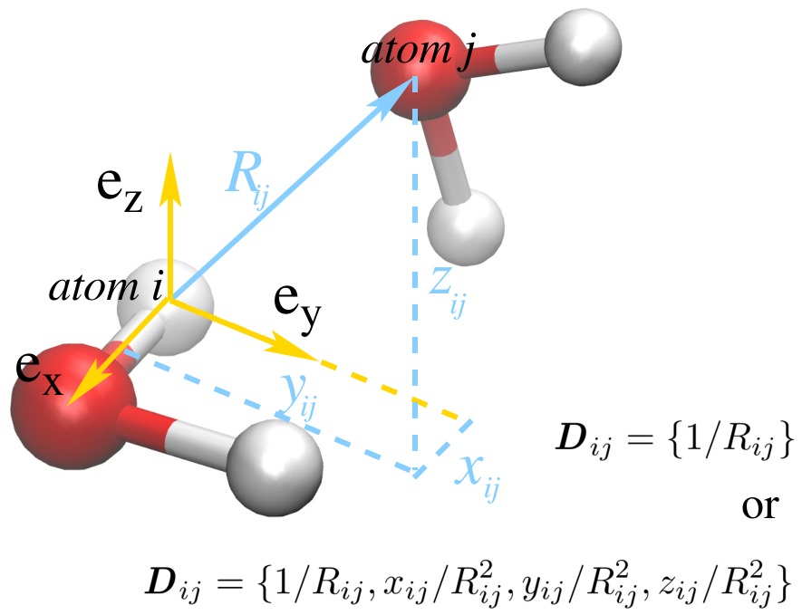
Figure 1: (color online). Schematic plot of the neural network input for the environment of atom $i$, taking water as an example. Atom $j$ is a generic neighbor of atom $i$. $(\textbf{{e}}_{x},\textbf{{e}}_{y},\textbf{{e}}_{z})$ is the local frame of atom $i$. $\textbf{{e}}_{x}$ is along the O-H bond. $\textbf{{e}}_{z}$ is perpendicular to the plane of the water molecule. $\textbf{{e}}_{y}$ is the cross product of $\textbf{{e}}_{z}$ and $\textbf{{e}}_{x}$. $(x_{ij},y_{ij},z_{ij})$ are the Cartesian components of the vector $\textbf{{R}}_{ij}$ in this local frame. $R_{ij}$ is the length of $\textbf{{R}}_{ij}$. The neural network input $\textbf{{D}}_{ij}$ may either contain the full radial and angular information of atom $j$, i.e., $\textbf{{D}}_{ij}=\{1/R_{ij},x_{ij}/R^{2}_{ij},y_{ij}/R^{2}_{ij},z_{ij}/R^{2}_{ij}\}$, or only the radial information, i.e., $\textbf{{D}}_{ij}=\{1/R_{ij}\}$. We first sort the neighbors of atom $i$ according to their chemical species, e.g. oxygens first then hydrogens. Within each species we sort the atoms according to their inverse distances to atom $i$, i.e., $1/R_{ij}$. We use $\{\textbf{{D}}_{ij}\}$ to denote the sorted input data for atom $i$.

图 1：（彩色在线）。以水为例，原子 $i$ 的环境作为神经网络输入的示意图。原子 $j$ 是原子 $i$ 的一个一般邻居。$(\textbf{{e}}_{x},\textbf{{e}}_{y},\textbf{{e}}_{z})$ 是原子 $i$ 的局域标架。$\textbf{{e}}_{x}$ 沿 O–H 键方向。$\textbf{{e}}_{z}$ 垂直于水分子平面。$\textbf{{e}}_{y}$ 是 $\textbf{{e}}_{z}$ 与 $\textbf{{e}}_{x}$ 的叉积。$(x_{ij},y_{ij},z_{ij})$ 是矢量 $\textbf{{R}}_{ij}$ 在该局域标架中的笛卡尔分量。$R_{ij}$ 是 $\textbf{{R}}_{ij}$ 的长度。神经网络输入 $\textbf{{D}}_{ij}$ 既可以包含原子 $j$ 的完整径向和角度信息，即 $\textbf{{D}}_{ij}=\{1/R_{ij},x_{ij}/R^{2}_{ij},y_{ij}/R^{2}_{ij},z_{ij}/R^{2}_{ij}\}$，也可以只包含径向信息，即 $\textbf{{D}}_{ij}=\{1/R_{ij}\}$。我们先按化学种类对原子 $i$ 的邻居排序，例如先氧后氢。在每一种类内部，再按它们到原子 $i$ 的倒数距离 $1/R_{ij}$ 排序。我们用 $\{ extbf{{D}}_{ij}\}$ 表示原子 $i$ 排好序的输入数据。

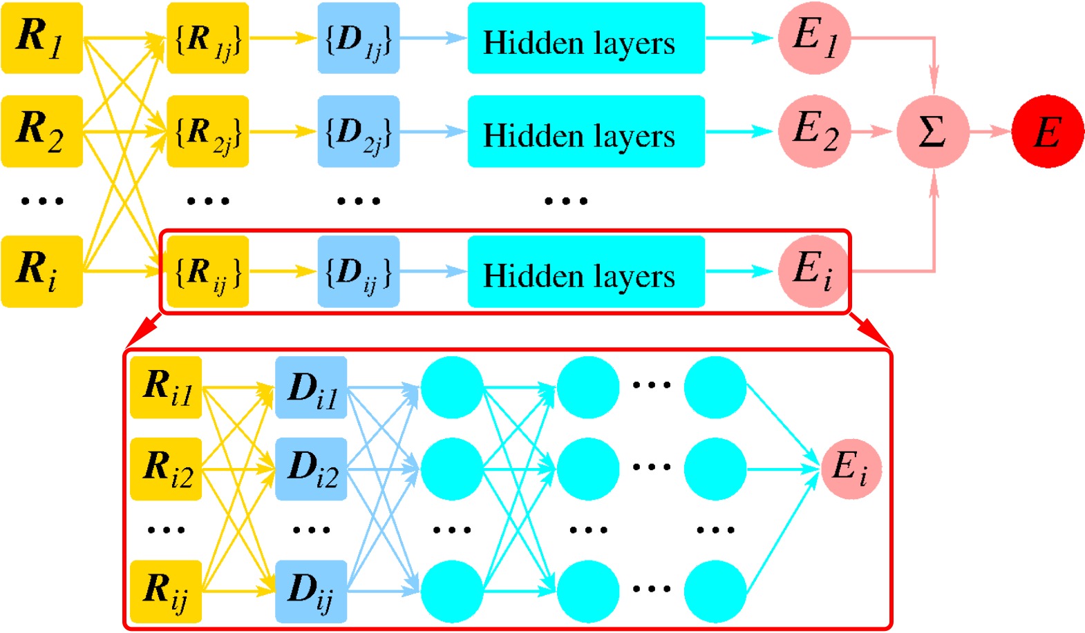
Figure 2: (color online). Schematic plot of the DeePMD model. The frame in the box is the zoom-in of a DNN. The relative positions of all neighbors w.r.t. atom $i$, i.e., $\{\textbf{{R}}_{ij}\}$, is first converted to $\{\textbf{{D}}_{ij}\}$, then passed to the hidden layers to compute $E_{i}$.

图 2：（彩色在线）。DeePMD 模型的示意图。方框中的部分是一个深度神经网络的放大。所有邻居相对于原子 $i$ 的相对位置 $\{ extbf{{R}}_{ij}\}$ 先被转换成 $\{ extbf{{D}}_{ij}\}$，再送入隐层以计算 $E_{i}$。

Next, $\{\textbf{{D}}_{ij}\}$ serves as input of a deep neural network (DNN) [22], which returns $E_{i}$ in output (Fig. 2). The DNN is a feed forward network, in which data flow from the input layer to the output layer ($E_{i}$), through multiple hidden layers consisting of several nodes that input the data $d^{\mathrm{in}}_{l}$ from the previous layer and output the data $d^{\mathrm{out}}_{k}$ to the next layer. A linear transformation is applied to the input data, i.e., $\tilde{d}_{k}=\sum_{l}w_{kl}d^{\mathrm{in}}_{l}+b_{k}$, followed by action of a non-linear function $\varphi$ on $\tilde{d}_{k}$, i.e., $d^{\mathrm{out}}_{k}=\varphi\big(\tilde{d}_{k}\big)$. In the final step from the last hidden layer to $E_{i}$, only the linear transformation is applied. The composition of the linear and nonlinear transformations introduced above provides the analytical representation of $E_{i}$ in terms of the local coordinates. The technical details of this construction are discussed in the supplementary materials (SM). In our applications, we adopt the hyperbolic tangent for $\varphi$ and use 5 hidden layers with decreasing number of nodes per layer, i.e., 240, 120, 60, 30, and 10 nodes, respectively, from the innermost to the outermost layer. It is known empirically that the hidden layers greatly enhance the capability of neural networks to fit complex and highly nonlinear functional dependences [23, 24]. In our case, only by including a few hidden layers could DeePMD reproduce the trajectories with sufficient accuracy.

接下来，$\{\textbf{{D}}_{ij}\}$ 作为深度神经网络（DNN）[22] 的输入，输出为 $E_{i}$（图 2）。该 DNN 是前馈网络，数据从输入层流到输出层（$E_{i}$），途经多个由若干节点组成的隐层；这些节点从前一层输入数据 $d^{\mathrm{in}}_{l}$，并向下一层输出数据 $d^{\mathrm{out}}_{k}$。先对输入数据做线性变换，即 $\tilde{d}_{k}=\sum_{l}w_{kl}d^{\mathrm{in}}_{l}+b_{k}$，再对 $\tilde{d}_{k}$ 作用非线性函数 $\varphi$，即 $d^{\mathrm{out}}_{k}=\varphi\big(\tilde{d}_{k}\big)$。从最后一个隐层到 $E_{i}$ 的最后一步，只做线性变换。上述线性和非线性变换的复合，给出了 $E_{i}$ 用局域坐标表示的解析形式。这一构造的技术细节在补充材料（SM）中讨论。在我们的应用中，$\varphi$ 采用双曲正切，并使用 5 个隐层，每层节点数递减，从最内层到最外层分别为 240、120、60、30 和 10 个节点。经验上已知，隐层会大大增强神经网络拟合复杂、高度非线性函数依赖的能力[23, 24]。在我们的情形中，只有加入若干隐层，DeePMD 才能以足够的精度复现轨迹。

We use the Adam method [5] to optimize the parameters $w_{kl}$ and $b_{k}$ of each layer with the family of loss functions

我们用 Adam 方法[5] 优化每一层的参数 $w_{kl}$ 和 $b_{k}$，所用的是如下一族损失函数

$$\displaystyle\hskip-11.38092ptL(p_{\epsilon},p_{f},p_{\xi})={p_{\epsilon}}\Delta\epsilon^{2}+\frac{p_{f}}{3N}\sum_{i}|\Delta\textbf{{F}}_{i}|^{2}+\frac{p_{\xi}}{9}||\Delta\xi||^{2}. \tag{1}$$

Here $\Delta$ denotes the difference between the DeePMD prediction and the training data, $N$ is the number of atoms, $\epsilon$ is the energy per atom, $\textbf{{F}}_{i}$ is the force on atom $i$, and $\xi$ is the virial tensor $\Xi=-\frac{1}{2}\sum_{i}\textbf{{R}}_{i}\otimes\textbf{{F}}_{i}$ divided by $N$. In Eq. (A13), $p_{\epsilon}$, $p_{f}$, and $p_{\xi}$ are tunable prefactors. When virial information is missing from the data, we set $p_{\xi}=0$. In order to minimize the loss function in Eq. (A13) in a well balanced way, we vary the magnitude of the prefactors during training. We progressively increase $p_{\epsilon}$ and $p_{\xi}$ and decrease $p_{f}$, so that the force term dominates at the beginning, while energy and virial terms become important at the end. We find that this strategy is very effective and reduces the total training time to a few core hours in all the test cases.

这里 $\Delta$ 表示 DeePMD 预测与训练数据之差，$N$ 是原子数，$\epsilon$ 是每个原子的能量，$\textbf{{F}}_{i}$ 是作用在原子 $i$ 上的力，$\xi$ 是维里张量 $\Xi=-\frac{1}{2}\sum_{i}\textbf{{R}}_{i}\otimes\textbf{{F}}_{i}$ 除以 $N$。在式(A13)中，$p_{\epsilon}$、$p_{f}$ 和 $p_{\xi}$ 是可调的前置因子。当数据中缺少维里信息时，我们取 $p_{\xi}=0$。为了以均衡的方式最小化式(A13)中的损失函数，我们在训练过程中改变这些前置因子的大小。我们逐步增大 $p_{\epsilon}$ 和 $p_{\xi}$，并减小 $p_{f}$，从而使力项在开始时占主导，而能量项和维里项在结束时变得重要。我们发现这一策略非常有效，在所有测试情形中都把总训练时间降到了几个核时。

To test the method, we have applied DeePMD to extended and finite systems. As representative extended systems, we consider (a) liquid water at $P$ = 1 bar and $T$ = 300 K, at the PI-AIMD level, (b) ice Ih at $P$ = 1 bar and $T$ = 273 K, at the PI-AIMD level, (c) ice Ih at $P$ = 1 bar and $T$ = 330 K, at the classical AIMD level, and (d) ice Ih at $P$ = 2.13 kbar and $T$ = 238 K, which is the experimental triple point for ice I, II, and III, at the classical AIMD level. The variable periodic simulation cell contains 64 H2O molecules in the case of liquid water, and 96 H2O molecules in the case of ices. We adopt $R_{c}$ = 6.0 Å and use the full radial and angular information for the 16 oxygens and the 32 hydrogens closest to the atom at the origin, while retaining only radial information for all the other atoms within $R_{c}$. All the ice simulations include proton disorder. Deuterons replace protons in the simulations (c) and (d). The PBE0+TS [26, 27] functional is adopted in all cases. As representative finite systems we consider benzene, uracil, napthalene, aspirin, salicylic acid, malonaldehyde, ethanol, and toluene, for which classical AIMD trajectories with the PBE+TS functional [28, 27] are available [^2]. In these systems, we set $R_{c}$ large enough to include all the atoms, and use the full radial and angular information in each local frame.

为了检验该方法，我们已把 DeePMD 应用到扩展体系和有限体系。作为有代表性的扩展体系，我们考虑：(a) $P$ = 1 bar、$T$ = 300 K 的液态水，在路径积分 AIMD 水平上；(b) $P$ = 1 bar、$T$ = 273 K 的冰 Ih，在路径积分 AIMD 水平上；(c) $P$ = 1 bar、$T$ = 330 K 的冰 Ih，在经典 AIMD 水平上；(d) $P$ = 2.13 kbar、$T$ = 238 K 的冰 Ih，这是冰 I、II 和 III 的实验三相点，在经典 AIMD 水平上。可变的周期性模拟原胞在液态水情形包含 64 个 H2O 分子，在冰的情形包含 96 个 H2O 分子。我们取 $R_{c}$ = 6.0 Å，对离原点最近的 16 个氧和 32 个氢使用完整的径向和角度信息，对 $R_{c}$ 内所有其他原子只保留径向信息。所有冰的模拟都包含质子无序。在模拟 (c) 和 (d) 中，氘核取代了质子。所有情形都采用 PBE0+TS[26, 27] 泛函。作为有代表性的有限体系，我们考虑苯、尿嘧啶、萘、阿司匹林、水杨酸、丙二醛、乙醇和甲苯，它们有采用 PBE+TS 泛函[28, 27] 的经典 AIMD 轨迹可用[^2]。在这些体系中，我们把 $R_{c}$ 取得足够大以包含全部原子，并在每个局域标架中使用完整的径向和角度信息。

We discuss the performance of DeePMD according to four criteria: ($i$) generality of the model; ($ii$) accuracy of the energy, forces, and virial tensor; ($iii$) faithfulness of the trajectories; ($iv$) scalability and computational cost. We refer to the SM for full details on the DeePMD implementation and the training datasets.

我们按四项准则讨论 DeePMD 的表现：($i$) 模型的普适性；($ii$) 能量、力和维里张量的准确性；($iii$) 轨迹的忠实程度；($iv$) 可扩展性与计算代价。关于 DeePMD 实现和训练数据集的完整细节，见补充材料。

$Generality$. Bulk and molecular systems exhibit different levels of complexity. The liquid water samples include quantum fluctuations. The organic molecules differ in composition and size, and the corresponding datasets include large numbers of conformations. Yet DeePMD produces satisfactory results in all cases, using the same methodology, network structure, and optimization scheme. The excellent performance of DeePMD in systems so diverse suggests that the method should be applicable to harder systems such as biological molecules, alloys, and liquid mixtures.

普适性。体相体系和分子体系呈现出不同层次的复杂性。液态水样本包含量子涨落。有机分子在组成和大小上各不相同，相应数据集包含大量构象。然而 DeePMD 在所有情形中都给出了令人满意的结果，所用的方法、网络结构和优化方案都相同。DeePMD 在如此多样的体系中的出色表现表明，该方法应当可以用于更困难的体系，例如生物分子、合金和液体混合物。

$Accuracy$. We quantify the accuracy of energy, forces, and virial predictions in terms of the root mean square error (RMSE) in the case of water and ices (Tab. 1), and in terms of the mean absolute error (MAE) in the case of the organic molecules (Tab. 2). No virial information was used for the latter. In the water case, the RMSE of the forces is comparable to the accuracy of the minimization procedure in the original AIMD simulations, in which the allowed error in the forces was less than $10^{-3}$ a.u.. In the case of the molecules, the predicted energy and forces are generally slightly better than the GDML benchmark.

准确性。对水和冰，我们用均方根误差（RMSE）来量化能量、力和维里预测的准确性（表 1）；对有机分子，则用平均绝对误差（MAE）（表 2）。后者没有使用维里信息。在水的情形中，力的 RMSE 与原来 AIMD 模拟中最小化手续的精度相当，那里允许的力误差小于 $10^{-3}$ a.u.。在分子的情形中，预测的能量和力一般略优于 GDML 基准。

System	Energy [meV]	Force [meV/Å]	Virial [meV]
liquid water	1.0	40.4	2.0
ice Ih (b)	0.7	43.3	1.5
ice Ih (c)	0.7	26.8	-
Ice Ih (d)	0.8	25.4	-

Table 1: The RMSE of the DeePMD prediction for water and ices in terms of the energy, the forces, and/or the virial. The RMSEs of the energy and the virial are normalized by the number of molecules in the system.

体系	能量 [meV]	力 [meV/Å]	维里 [meV]
液态水	1.0	40.4	2.0
冰 Ih (b)	0.7	43.3	1.5
冰 Ih (c)	0.7	26.8	-
冰 Ih (d)	0.8	25.4	-

表 1：DeePMD 对水和冰在能量、力和/或维里上的预测 RMSE。能量和维里的 RMSE 按体系中的分子数做了归一。

Molecule	Energy [meV]	Force [meV/Å]
Benzene	2.8 (3.0)	7.6 (10.0)
Uracil	3.7 (4.0)	9.8 (10.4)
Naphthalene	4.1 (5.2)	7.1 (10.0)
Aspirin	8.7 (11.7)	19.1 (42.9)
Salicylic acid	4.6 (5.2)	10.9 (12.1)
Malonaldehyde	4.0 (6.9)	12.7 (34.7)
Ethanol	2.4 (6.5)	8.3 (34.3)
Toluene	3.7 (5.2)	8.5 (18.6)

Table 2: The MAE of the DeePMD prediction for organic molecules in terms of the energy and the forces. The numbers in parentheses are the GDML results [19].

分子	能量 [meV]	力 [meV/Å]
苯	2.8 (3.0)	7.6 (10.0)
尿嘧啶	3.7 (4.0)	9.8 (10.4)
萘	4.1 (5.2)	7.1 (10.0)
阿司匹林	8.7 (11.7)	19.1 (42.9)
水杨酸	4.6 (5.2)	10.9 (12.1)
丙二醛	4.0 (6.9)	12.7 (34.7)
乙醇	2.4 (6.5)	8.3 (34.3)
甲苯	3.7 (5.2)	8.5 (18.6)

表 2：DeePMD 对有机分子在能量和力上的预测 MAE。括号中的数字是 GDML 的结果[19]。

$MD$ $trajectories$. In the case of water and ices, we perform path-integral/classical DeePMD simulations at the thermodynamic conditions of the original models, using the i-PI software [2], but with much longer simulation time (300 $ps$). The average energy $\bar{E}$, density $\bar{\rho}$, radial distribution functions (RDFs), and a representative angular distribution function (ADF), i.e., a 3-body correlation function, are reproduced with high accuracy. The results are summarized in Tab. 3. The RDFs and ADF of the quantum trajectories of water are shown in Fig. 3. The RDFs of ice are reported in the SM. A higher-order correlation function, the probability distribution function of the O-O bond orientation order parameter $Q_{6}$, is additionally reported in the SM and shows excellent agreement between DeePMD and AIMD trajectories. In the case of the molecules, we perform DeePMD at the same temperature of the original data, using a Langevin thermostat with a damping time $\tau$ = 0.1 ps. The corresponding distributions of interatomic distances are very close to the original data (Fig. 4).

MD 轨迹。对水和冰，我们在原模型的热力学条件下，用 i-PI 软件[2] 进行路径积分/经典 DeePMD 模拟，但模拟时间长得多（300 ps）。平均能量 $\bar{E}$、密度 $\bar{\rho}$、径向分布函数（RDF）以及一个有代表性的角分布函数（ADF），也就是一种三体关联函数，都被高精度地复现。结果汇总于表 3。水的量子轨迹的 RDF 和 ADF 示于图 3。冰的 RDF 见补充材料。一种更高阶的关联函数，即 O–O 键取向序参量 $Q_{6}$ 的概率分布函数，也在补充材料中给出，并显示出 DeePMD 与 AIMD 轨迹之间很好的一致。对分子，我们在与原数据相同的温度下做 DeePMD，使用阻尼时间 $\tau$ = 0.1 ps 的 Langevin 热浴。相应的原子间距分布与原数据非常接近（图 4）。

System	$\bar{E}$[eV/H2O]	$\bar{\rho}$[g/m3]
liquid water	-467.678(2) [-467.679(6)]	1.013(5) [1.013(20)]
ice Ih (b)	-467.750(1) [-467.747(4)]	0.967(1) [0.966(6)]
ice Ih (c)	-468.0478(3) [-468.0557(16)]	0.950(1) [0.949(2)]
ice Ih (d)	-468.0942(2) [-468.1026(9)]	0.986(1) [0.985(2)]

Table 3: The equilibrium energy and density, $\bar{E}$ and $\bar{\rho}$, of water and ices, with DeePMD and AIMD. The numbers in square brackets are the AIMD results. The numbers in parentheses are statistical uncertainties in the last one or two digits. The training AIMD trajectories for the ices are shorter and more correlated than in the water case.

体系	$\bar{E}$[eV/H2O]	$\bar{\rho}$[g/m3]
液态水	-467.678(2) [-467.679(6)]	1.013(5) [1.013(20)]
冰 Ih (b)	-467.750(1) [-467.747(4)]	0.967(1) [0.966(6)]
冰 Ih (c)	-468.0478(3) [-468.0557(16)]	0.950(1) [0.949(2)]
冰 Ih (d)	-468.0942(2) [-468.1026(9)]	0.986(1) [0.985(2)]

表 3：水和冰的平衡能量与密度 $\bar{E}$ 和 $\bar{\rho}$，分别给出 DeePMD 和 AIMD 的结果。方括号中的数字是 AIMD 结果。圆括号中的数字是末一位或两位的统计不确定度。用于训练的冰的 AIMD 轨迹比水的情形更短，也更相关。

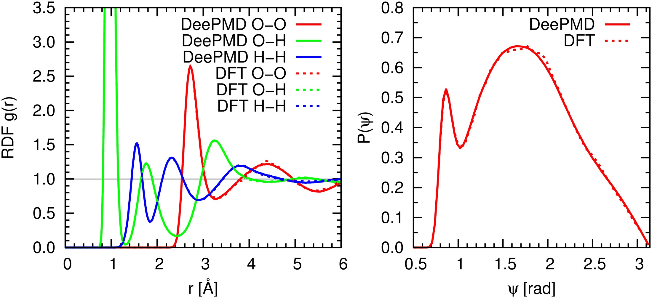
Figure 3: Correlation functions of liquid water from DeePMD and PI-AIMD. Left: RDFs. Right: the O-O-O ADF within a cutoff radius of 3.7 Å.

图 3：DeePMD 与路径积分 AIMD 得到的液态水关联函数。左：径向分布函数。右：截断半径 3.7 Å 内的 O–O–O 角分布函数。

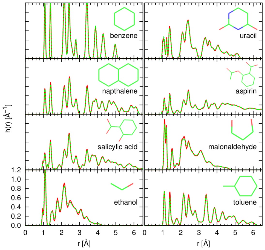
Figure 4: Interatomic distance distributions of the organic molecules. The solid lines denote the DeePMD results. The dashed lines denote the AIMD results.

图 4：有机分子的原子间距分布。实线表示 DeePMD 结果。虚线表示 AIMD 结果。

$Scalability$ $and$ $computational$ $cost$. All the physical quantities in DeePMD are sums of local contributions. Thus, after training on a relatively small system, DeePMD can be directly applied to much larger systems. The computational cost of DeePMD scales linearly with the number of atoms. Moreover, DeePMD can be easily parallelized due to its local decomposition and the near-neighbor dependence of its “atomic energies”. In Fig. 5, we compare the cost of DeePMD fixed-cell simulations ($NVT$) of liquid water with that of equivalent simulations with AIMD and the empirical FF TIP3P [30] in units of CPU core seconds/step/molecule.

可扩展性与计算代价。DeePMD 中的所有物理量都是局域贡献之和。因此，在相对较小的体系上训练之后，DeePMD 可以直接应用到大得多的体系。DeePMD 的计算代价随原子数线性增长。此外，由于其局域分解以及“原子能量”对近邻的依赖，DeePMD 很容易并行化。在图 5 中，我们把液态水的 DeePMD 固定原胞模拟（$NVT$）的代价，与同等的 AIMD 以及经验力场 TIP3P[30] 模拟的代价加以比较，单位是 CPU 核秒/步/分子。

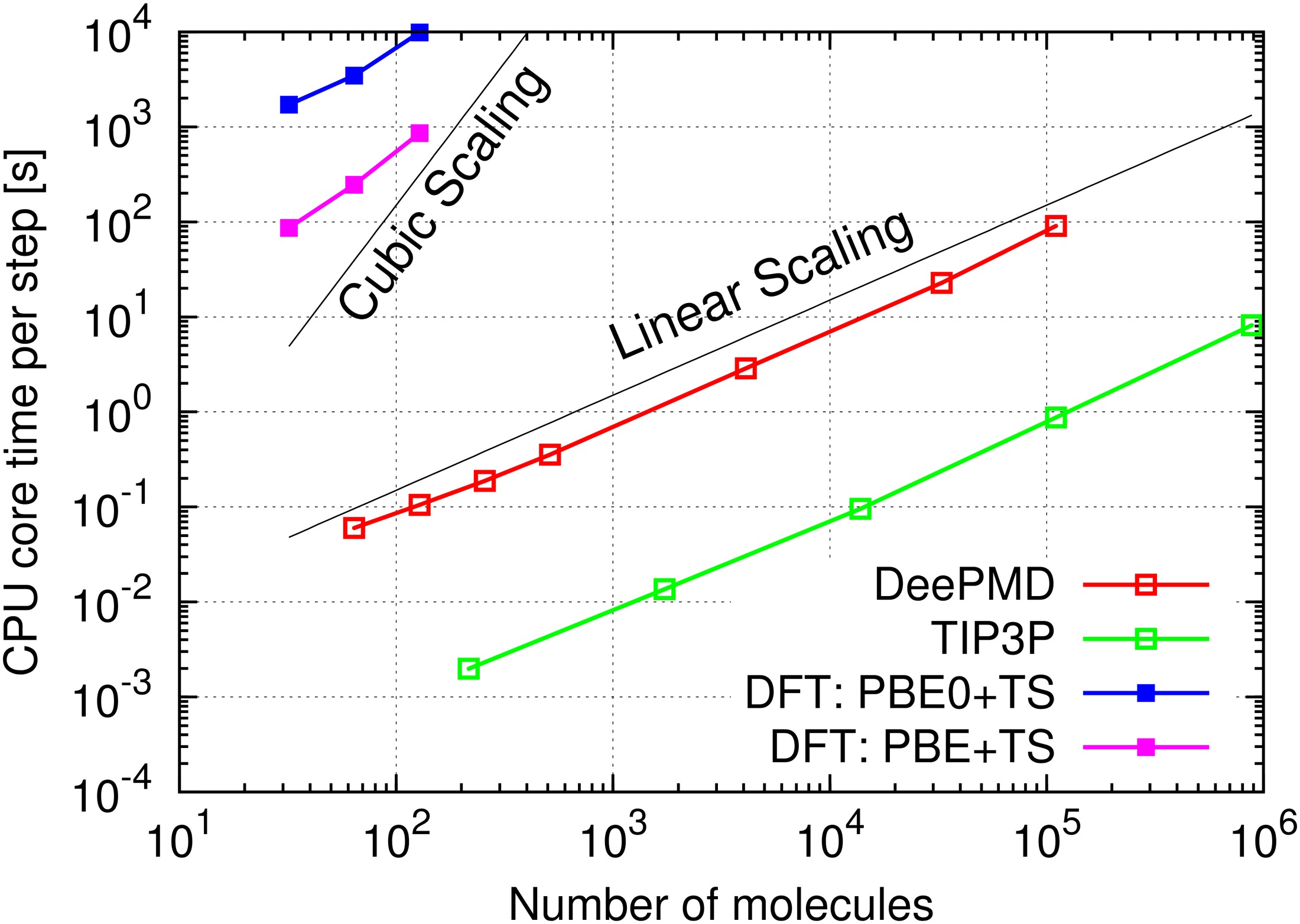
Figure 5: Computational cost of MD step $vs.$ system size, with DeePMD, TIP3P, PBE+TS and, PBE0+TS. All simulations are performed on a Nersc Cori supercomputer with the Intel Xeon CPU E5-2698 v3. The TIP3P simulations use the Gromacs codes (version 4.6.7) [31]. The PBE+TS and PBE0+TS simulations use the Quantum Espresso codes [32].

图 5：分子动力学单步计算代价随体系规模的变化，比较对象为 DeePMD、TIP3P、PBE+TS 和 PBE0+TS。所有模拟都在 Nersc Cori 超级计算机上、使用 Intel Xeon CPU E5-2698 v3 进行。TIP3P 模拟使用 Gromacs 程序（4.6.7 版）[31]。PBE+TS 和 PBE0+TS 模拟使用 Quantum Espresso 程序[32]。

While in principle the environmental dependence of $E_{i}$ is analytical, in our implementation discontinuities are present in the forces, due to adoption of a sharp cutoff radius, limitation of angular information to a fixed number of atoms, and abrupt changes in the atomic lists due to sorting. These discontinuities are similar in magnitude to those present in the AIMD forces due to finite numerical accuracy in the enforcement of the Born-Oppenheimer condition. In both cases, the discontinuities are much smaller than thermal fluctuations and perfect canonical evolution is achieved by coupling the systems to a thermostat. We further note that long-range Coulomb interactions are not treated explicitly in the current implementation, although implicitly present in the training data. Explicit treatment of Coulombic effects may be necessary in some applications and deserves further study.

虽然原则上 $E_{i}$ 对环境的依赖是解析的，但在我们的实现中，力存在间断，原因是采用了尖锐的截断半径、把角度信息限制在固定数目的原子上，以及排序造成的原子列表突变。这些间断的幅度，与 AIMD 中因玻恩–奥本海默条件只能以有限数值精度施加而产生的力的间断相当。在这两种情形里，间断都远小于热涨落，把体系与热浴耦合后即可得到完善的正则演化。我们还要指出，当前实现中没有显式处理长程库仑相互作用，尽管它们隐含在训练数据中。在某些应用中，可能需要显式处理库仑效应，这值得进一步研究。

In conclusion, DeePMD realizes a paradigm for molecular simulation, wherein accurate quantum mechanical data are faithfully parametrized by machine learning algorithms, which make possible simulations of DFT based AIMD quality on much larger systems and for much longer time than with direct AIMD. While substantially more predictive than empirical FFs, DFT is not chemically accurate [^3]. In principle DeePMD could be trained with chemically accurate data from high-level quantum chemistry [33] and/or quantum Monte Carlo [34], but so far this has been prevented by the large computational cost of these calculations.

总之，DeePMD 实现了一种分子模拟范式：准确的量子力学数据被机器学习算法忠实地参数化，从而使基于 DFT 的、具有 AIMD 品质的模拟，能够在比直接 AIMD 大得多的体系和长得多的时间上进行。尽管比经验力场更有预测力，DFT 并未达到化学精度[^3]。原则上，DeePMD 可以用高水平量子化学[33]和/或量子蒙特卡罗[34]的具有化学精度的数据来训练，但迄今为止，这些计算的巨大代价阻止了这一点。

DeePMD should also very useful to coarse grain the atomic degrees of freedom, for example, by generating an NN model for a reduced set of degrees of freedom while using the full set of degrees of freedom for training. The above considerations suggest that DeePMD should enhance considerably the realm of AIMD applications by successfully addressing the dilemma of accuracy versus efficiency that has confronted the molecular simulation community for a long time.

DeePMD 对原子自由度的粗粒化也应当非常有用，例如，对一组约化的自由度生成神经网络模型，同时用完整的自由度来训练。上述考虑表明，DeePMD 应当能显著拓展 AIMD 的应用范围，从而较好地应对分子模拟界长期面临的准确性与效率之间的两难。

[^1] Some flexibility can be used in the definition of the local frame of atom $i$. Usually we define it in terms of the two atoms closest to $i$, independently of their species. Exceptions to this rule are discussed in the SM.

[^1] 在定义原子 $i$ 的局域标架时，可以有一定灵活性。通常我们用离 $i$ 最近的两个原子来定义，而不论它们的种类。对这一规则的例外在补充材料中讨论。

[^2] http://quantum-machine.org/

[^3] Conventionally, chemical accuracy corresponds to an error of 1 kcal/mol in the energy.

[^3] 按惯例，化学精度对应于能量误差为 1 kcal/mol。

References

参考文献

[1] R. Car and M. Parrinello, Physical Review Letters 55 , 2471 (1985).

[2] D. Marx and J. Hutter, Ab initio molecular dynamics: basic theory and advanced methods (Cambridge University Press, 2009).

[3] W. Kohn and L. J. Sham, Physical Review 140 , A1133 (1965).

[4] K. Vanommeslaeghe, E. Hatcher, C. Acharya, S. Kundu, S.and Zhong, J. Shim, E. Darian, O. Guvench, P. Lopes, I. Vorobyov, and A. Mackerell Jr., Journal of Computational Chemistry 31 , 671 (2010).

[5] W. Jorgensen, D. Maxwell, and J. Tirado-Rives, Journal of the American Chemical Society 118 , 11225 (1996).

[6] J. Wang, R. M. Wolf, J. W. Caldwell, P. A. Kollman, and D. A. Case, Journal of Computational Chemistry 25 , 1157 (2004).

[7] F. H. Stillinger and T. A. Weber, Physical Review B 31 , 5262 (1985).

[8] M. S. Daw and M. I. Baskes, Physical Review B 29 , 6443 (1984).

[9] D. W. Brenner, O. A. Shenderova, J. A. Harrison, S. J. Stuart, B. Ni, and S. B. Sinnott, Journal of Physics: Condensed Matter 14 , 783 (2002).

[10] A. C. Van Duin, S. Dasgupta, F. Lorant, and W. A. Goddard, The Journal of Physical Chemistry A 105 , 9396 (2001).

[11] A. P. Thompson, L. P. Swiler, C. R. Trott, S. M. Foiles, and G. J. Tucker, Journal of Computational Physics 285 , 316 (2015).

[12] T. D. Huan, R. Batra, J. Chapman, S. Krishnan, L. Chen, and R. Ramprasad, NPJ Computational Materials 3 , 1 (2017).

[13] J. Behler and M. Parrinello, Physical Review Letters 98 , 146401 (2007).

[14] J. Behler, The Journal of Chemical Physics 145 , 170901 (2016).

[15] T. Morawietz, A. Singraber, C. Dellago, and J. Behler, Proceedings of the National Academy of Sciences , 201602375 (2016).

[16] A. P. Bartók, M. C. Payne, R. Kondor, and G. Csányi, Physical Review Letters 104 , 136403 (2010).

[17] M. Rupp, A. Tkatchenko, K.-R. Müller, and O. A. VonLilienfeld, Physical Review Letters 108 , 058301 (2012).

[18] K. T. Schütt, F. Arbabzadah, S. Chmiela, K. R. Müller, and A. Tkatchenko, Nature Communications 8 , 13890 (2017).

[19] S. Chmiela, A. Tkatchenko, H. E. Sauceda, I. Poltavsky, K. T. Schütt, and K.-R. Müller, Science Advances 3 , e1603015 (2017).

[20] J. S. Smith, O. Isayev, and A. E. Roitberg, Chemical Science 8 , 3192 (2017).

[21] J. Han, L. Zhang, R. Car, and W. E, Communications in Computational Physics 23 , 629 (2018).

[22] I. Goodfellow, Y. Bengio, and A. Courville, Deep learning (MIT Press, 2016).

[23] Y. Bengio, P. Lamblin, D. Popovici, and H. Larochelle, in Advances in neural information processing systems (2007) pp. 153–160.

[24] A. Krizhevsky, I. Sutskever, and G. E. Hinton, in Advances in neural information processing systems (2012) pp. 1097–1105.

[25] D. Kingma and J. Ba, in Proceedings of the International Conference on Learning Representations (ICLR) (2015).

[26] C. Adamo and V. Barone, The Journal of Chemical Physics 110 , 6158 (1999).

[27] A. Tkatchenko and M. Scheffler, Physical Review Letters 102 , 073005 (2009).

[28] J. P. Perdew, K. Burke, and M. Ernzerhof, Physical Review Letters 77 , 3865 (1996).

[29] M. Ceriotti, J. More, and D. E. Manolopoulos, Computer Physics Communications 185 , 1019 (2014).

[30] W. L. Jorgensen, J. Chandrasekhar, J. D. Madura, R. W. Impey, and M. L. Klein, The Journal of Chemical Physics 79 , 926 (1983).

[31] S. Pronk, S. Páll, R. Schulz, P. Larsson, P. Bjelkmar, R. Apostolov, M. Shirts, J. Smith, P. Kasson, D. van der Spoel, B. Hess, and E. Lindahl, Bioinformatics , btt055 (2013).

[32] O. Andreussi, T. Brumme, O. Bunau, M. B. Nardelli, M. Calandra, R. Car, C. Cavazzoni, D. Ceresoli, M. Cococcioni, N. Colonna, et al. , Journal of Physics: Condensed Matter (2017).

[33] J. D. Watts, J. Gauss, and R. J. Bartlett, The Journal of Chemical Physics 98 , 8718 (1993).

[34] D. Ceperley and B. Alder, Science 231 (1986).

Appendix A Supplementary Materials

附录 A 补充材料

A.1 Training/Testing Data

A.1 训练/测试数据

A.1.1 water and ice

The data used for training and/or testing are extracted from the AIMD simulations summarized in Tab. 4. All the simulations adopt a time step of 0.48 fs. The PI-AIMD simulations use the CPMD codes of Quantum Espresso [^4] for the DFT part and are interfaced with the i-PI code [2] for the path-integral part. The generalized Langevin equation with color noise [1] in i-PI requires 8 beads for a converged representation of the Feynman paths. The classical AIMD simulations use the CPMD codes of Quantum Espresso and adopt the Nosé-Hoover thermostat [7] for thermalization. The Parrinello-Rahman technique [8] for variable cell dynamics is adopted in all cases. The training datasets include 95000 snapshots (from 105000 total snapshots) randomly selected along the liquid water trajectory, 19500 snapshots (from 24000 total snapshots) randomly selected along the ice (b) trajectory, 9500 snapshots (from 12000 total snapshots) randomly selected along the ice (c) trajectory, and 9500 snapshots (from 12000 total snapshots) randomly selected along the ice (d) trajectory. The remaining snapshots in the database are used for testing purposes.

A.1.1 水和冰

用于训练和/或测试的数据，取自表 4 所汇总的 AIMD 模拟。所有模拟的时间步长均为 0.48 fs。路径积分 AIMD 模拟在 DFT 部分使用 Quantum Espresso 的 CPMD 程序[^4]，并与 i-PI 程序[2] 接口以处理路径积分部分。i-PI 中带有有色噪声的广义 Langevin 方程[1] 需要 8 个珠子，才能给出费曼路径的收敛表示。经典 AIMD 模拟使用 Quantum Espresso 的 CPMD 程序，并用 Nosé–Hoover 热浴[7] 做热化。所有情形都采用用于变原胞动力学的 Parrinello–Rahman 技术[8]。训练数据集包括：沿液态水轨迹随机选取的 95000 帧（总共 105000 帧），沿冰 (b) 轨迹随机选取的 19500 帧（总共 24000 帧），沿冰 (c) 轨迹随机选取的 9500 帧（总共 12000 帧），以及沿冰 (d) 轨迹随机选取的 9500 帧（总共 12000 帧）。数据库中其余帧用于测试。

System	PI/classical	$N$	$P$ [bar]	$T$ [K]	traj. length [ps]
LW	path integral	64	1.0	300	6.2
ice (b)	path integral	96	1.0	273	1.5
ice (c)	classical	96	1.0	330	6.0
ice (d)	classical	96	2.13k	238	6.0

Table 4: Equilibrated AIMD trajectories (traj.) for liquid water (LW) and ice Ih.

体系	路径积分/经典	$N$	$P$ [bar]	$T$ [K]	轨迹长度 [ps]
液态水	路径积分	64	1.0	300	6.2
冰 (b)	路径积分	96	1.0	273	1.5
冰 (c)	经典	96	1.0	330	6.0
冰 (d)	经典	96	2.13k	238	6.0

表 4：液态水（LW）和冰 Ih 的已平衡 AIMD 轨迹。

A.1.2 molecules

The data and their complete description for the organic molecules (benzene, uracil, napthalene, aspirin, salicylic acid, malonaldehyde, ethanol, and toluene) can be found at http://quantum-machine.org/. For each molecule, 95000 snapshots, randomly selected from the database, are used to train the DeePMD model. The remaining snapshots in the database are used for testing purposes.

A.1.2 分子

有机分子（苯、尿嘧啶、萘、阿司匹林、水杨酸、丙二醛、乙醇和甲苯）的数据及其完整说明，可见于 http://quantum-machine.org/。对每个分子，从数据库中随机选取 95000 帧来训练 DeePMD 模型。数据库中其余帧用于测试。

A.2 Implementation of the method

A.2 方法的实现

The TensorFlow r1.0 software library  (http://tensorflow.org/) is interfaced with our C++ codes for data training and for calculating the energy, the forces, and the virial.

TensorFlow r1.0 软件库（http://tensorflow.org/）与我们用于数据训练以及计算能量、力和维里的 C++ 代码相接口。

A.2.1 network input data

We consider a system consisting of $N$ atoms. The global coordinates of the atoms, in the laboratory frame, are $\left\{\bm{R}_{1},\bm{R}_{2},\dots,\bm{R}_{N}\right\}$, where $\bm{R}_{i}=\left\{x_{i},y_{i},z_{i}\right\}$ for each $i$. The neighbors of atom $i$ are denoted by $\mathcal{N}(i)=\left\{j:|\bm{R}_{ij}|<R_{c}\right\}$, where $\bm{R}_{ij}=\bm{R}_{i}-\bm{R}_{j}$, and $R_{c}$ is the cut-off radius. The neighbor list $\mathcal{N}(i)$ is sorted according to the scheme illustrated in Fig. 1. In extended systems, the number of neighbors at different snapshots inside $R_{c}$ fluctuates. Let $N_{c}$ be the largest fluctuating number of neighbors. The two atoms used to define the axes of the local frame of atom $i$ are called the axis-atoms and are denoted by $a(i)\in\mathcal{N}(i)$ and $b(i)\in\mathcal{N}(i)$, respectively. In general we choose two closest atoms, independently of their species, together with the center atom, to define the local frame. Thus, in all the water cases, we choose the other two atoms belonging to the same water molecule. We apply the same rule to the organic molecules, but in this case we exclude the hydrogen atoms in the definition of the axis-atoms.

A.2.1 网络输入数据

我们考虑由 $N$ 个原子组成的体系。实验室标架中原子的整体坐标为 $\left\{\bm{R}_{1},\bm{R}_{2},\dots,\bm{R}_{N}\right\}$，对每个 $i$ 有 $\bm{R}_{i}=\left\{x_{i},y_{i},z_{i}\right\}$。原子 $i$ 的邻居记为 $\mathcal{N}(i)=\left\{j:|\bm{R}_{ij}|<R_{c}\right\}$，其中 $\bm{R}_{ij}=\bm{R}_{i}-\bm{R}_{j}$，$R_{c}$ 是截断半径。邻居列表 $\mathcal{N}(i)$ 按图 1 所示方案排序。在扩展体系中，$R_{c}$ 内的邻居数目在不同帧之间会涨落。设 $N_{c}$ 为涨落的邻居数的最大值。用于定义原子 $i$ 局域标架坐标轴的两个原子称为轴原子，分别记为 $a(i)\in\mathcal{N}(i)$ 和 $b(i)\in\mathcal{N}(i)$。一般地，我们选取两个最近的原子（不论种类），连同中心原子一起来定义局域标架。因此，在所有水的情形中，我们选取属于同一水分子的另外两个原子。我们对有机分子采用同一规则，但在定义轴原子时排除氢原子。

Next, we define the rotation matrix $\mathcal{R}(\bm{R}_{ia(i)},\bm{R}_{ib(i)})$ for the local frame of atom $i$,

接下来，我们定义原子 $i$ 局域标架的旋转矩阵 $\mathcal{R}(\bm{R}_{ia(i)},\bm{R}_{ib(i)})$，

$$\displaystyle\mathcal{R}(\bm{R}{ia(i)},\bm{R}{ib(i)})=\begin{pmatrix}\bm{e}[\bm{R}{ia(i)}]\
\bm{e}[\bm{R}{ib(i)}-(\bm{R}{ia(i)}\cdot\bm{R}{ib(i)}\bm{R}{ia(i)}]\
\bm{e}[\bm{R}{ia(i)}\times\bm{R}_{ib(i)}]\end{pmatrix}^{T}, \tag{2}$$

where $\bm{e}[\bm{x}]\equiv\frac{\bm{x}}{||\bm{x}||}$. In this local frame of reference, we obtain the new set of coordinates:

其中 $\bm{e}[\bm{x}]\equiv\frac{\bm{x}}{||\bm{x}||}$。在这一局域参考系中，我们得到新的坐标集合：

$$\displaystyle\bm{R}_{ij}^{\prime}=\left\{x_{ij}^{\prime},y_{ij}^{\prime},z_{ij}^{\prime}\right\}=\left\{x_{ij},y_{ij},z_{ij}\right\}\mathcal{R}(\bm{R}_{ia(i)},\bm{R}_{ib(i)}), \tag{3}$$

and we define $R_{ij}^{\prime}=||\bm{R}_{ij}^{\prime}||$. Then the spacial information for $j\in\mathcal{N}(i)$ is

并定义 $R_{ij}^{\prime}=||\bm{R}_{ij}^{\prime}||$。于是，对 $j\in\mathcal{N}(i)$，空间信息为

$$\displaystyle\bm{D}{ij}\equiv\begin{cases}\left{D{ij}^{0},D_{ij}^{1},D_{ij}^{2},D_{ij}^{3}\right}=\left{\frac{1}{R_{ij}^{\prime}},\frac{x_{ij}^{\prime}}{R_{ij}^{\prime 2}},\frac{y_{ij}^{\prime}}{R_{ij}^{\prime 2}},\frac{z_{ij}^{\prime}}{R_{ij}^{\prime 2}}\right},&\text{full radial and angular information;}\
\left{D_{ij}^{0}\right}=\left{\frac{1}{R_{ij}^{\prime}}\right},&\text{radial information only.}\end{cases}$$

When $\alpha=0,1,2,3$, full (radial plus angular) information is provided. When $\alpha=0$, only radial information is used. Note that for $j\in\mathcal{N}(i)$, $D_{ij}^{\alpha}$ is a function of the global coordinates of three or four atoms:

当 $\alpha=0,1,2,3$ 时，提供的是完整（径向加角度）信息。当 $\alpha=0$ 时，只使用径向信息。注意，对 $j\in\mathcal{N}(i)$，$D_{ij}^{\alpha}$ 是三个或四个原子整体坐标的函数：

$\displaystyle D_{ij}^{\alpha}=\begin{cases}D_{ij}^{\alpha}(\bm{R}_{i},\bm{R}_{a(i)},\bm{R}_{b(i)}),&\text{forj=a(i)$or$j=b(i)$};\
D_{ij}^{\alpha}(\bm{R}{i},\bm{R}{a(i)},\bm{R}{b(i)},\bm{R}{j}),&\text{otherwise}.\end{cases}$$

This formula is useful in the derivation of the formulae for the forces and the virial tensor given below.

这一公式在下面推导力和维里张量的公式时很有用。

The neural network uses a fixed input data size. Thus, when the size of $\mathcal{N}(i)$ is smaller than $N_{c}$, we temporarily set to zero the input nodes not used for storing the $D_{ij}^{\alpha}$. The nodes set to zero are still labeled by $D_{ij}^{\alpha}$.

神经网络使用固定的输入数据尺寸。因此，当 $\mathcal{N}(i)$ 的大小小于 $N_{c}$ 时，我们暂时把那些不用于存储 $D_{ij}^{\alpha}$ 的输入节点置零。这些被置零的节点仍用 $D_{ij}^{\alpha}$ 来标记。

The $D_{ij}^{\alpha}$ are then standardized to be the input data for the neural networks. In this procedure, the $D_{ij}^{\alpha}$ are grouped according to the different atomic species. Within each group we calculate the mean and standard deviation of each $D_{ij}^{\alpha}$ by averaging over the snapshots of the training sample and over all the atoms in the group. Then we shift the $D_{ij}^{\alpha}$ by their corresponding means, and divide them by their corresponding standard deviations. Because of the weight $1/R$ in the $D_{ij}^{\alpha}$ and because the unoccupied nodes are set to zero, some standard deviations are very small or even zero. This causes an ill-posed training process. Therefore, after the shift operations, we divide by 0.01 Å*-1* the $D_{ij}^{\alpha}$ with standard deviation smaller than 0.01 Å*-1*. For simplicity, we still use the same notation for the standardized $D_{ij}^{\alpha}$.

随后对 $D_{ij}^{\alpha}$ 做标准化，作为神经网络的输入数据。在这一手续中，$D_{ij}^{\alpha}$ 按不同原子种类分组。在每一组内，我们通过对训练样本的各帧以及组内所有原子求平均，计算每个 $D_{ij}^{\alpha}$ 的均值和标准差。然后把 $D_{ij}^{\alpha}$ 减去相应的均值，再除以相应的标准差。由于 $D_{ij}^{\alpha}$ 中的权重 $1/R$，以及未占用节点被置零，有些标准差会非常小甚至为零。这会导致病态的训练过程。因此，在平移操作之后，对标准差小于 0.01 Å$^{-1}$ 的 $D_{ij}^{\alpha}$，我们改用 0.01 Å$^{-1}$ 来除。为简单起见，标准化后的 $D_{ij}^{\alpha}$ 仍使用同一记号。

A.2.2 deep neural network for the energy

For atom $i$, the “atomic energy” is represented as

A.2.2 用于能量的深度神经网络

对原子 $i$，“原子能量”表示为

$$\displaystyle E_{i}=N_{\bm{w}(i)}(\{D_{ij}^{\alpha}\}_{j\in\mathcal{N}(i),\alpha}), \tag{4}$$

where $N_{\bm{w}(i)}$ is the network that computes the atomic contribution to the total energy, and $\bm{w}(i)$ are the weights used to parametrize the network, which depend on the chemical species of atom $i$.

其中 $N_{\bm{w}(i)}$ 是计算总能量中该原子贡献的网络，$\bm{w}(i)$ 是用来参数化该网络的权重，它们依赖于原子 $i$ 的化学种类。

In this work, $N_{\bm{w}(i)}$ is constructed as a feedforward network in which data flows from the input layer as $\{D_{ij}^{\alpha}\}$, through multiple fully connected hidden layers, to the output layer as the atomic energy $E_{i}$. More specifically, a feedforward neural network with $N_{h}$ hidden layers is a mapping

在本工作中，$N_{\bm{w}(i)}$ 被构造成一个前馈网络，数据从作为 $\{D_{ij}^{\alpha}\}$ 的输入层，经过多个全连接隐层，流到作为原子能量 $E_{i}$ 的输出层。更具体地说，一个有 $N_{h}$ 个隐层的前馈神经网络是如下映射

$$\displaystyle\mathcal{N}_{i}(\{D_{ij}^{\alpha}\})=\mathcal{L}^{\mathrm{out}}_{i}\circ\mathcal{L}_{i}^{N_{h}}\circ\mathcal{L}_{i}^{N_{h}-1}\circ\cdots\circ\mathcal{L}_{i}^{1}(\{D_{ij}^{\alpha}\}), \tag{5}$$

where the symbol “$\circ$” denotes function composition. Here $\mathcal{L}_{i}^{p}$ is the mapping from layer $p-1$ to $p$, a composition of a linear transformation and a non-linear transformation

其中符号 “$\circ$” 表示函数复合。这里 $\mathcal{L}_{i}^{p}$ 是从第 $p-1$ 层到第 $p$ 层的映射，由一个线性变换和一个非线性变换复合而成

$$\textbf{{d}}_{i}^{p}=\mathcal{L}_{i}^{p}(\textbf{{d}}_{i}^{p-1})=\varphi\big(\textbf{{W}}_{i}^{p}\textbf{{d}}_{i}^{p-1}+\textbf{{b}}_{i}^{p}\big). \tag{6}$$

The $\textbf{{d}}^{p}_{i}\in\mathbb{R}^{M_{p}}$ denote the values of neurons in layer $p$ and $M_{p}$ the number of neurons. The weight matrix $\textbf{{W}}_{i}^{p}\in\mathbb{R}^{M_{p}\times M_{p-1}}$ and bias vector $\textbf{{b}}_{i}^{p}\in\mathbb{R}^{M_{p}}$ are free parameters of the linear transformation that are to be optimized. The non-linear activation function $\varphi$ is in general a component-wise function, and here it is taken to be the hyperbolic tangent, i.e.,

$\textbf{{d}}^{p}_{i}\in\mathbb{R}^{M_{p}}$ 表示第 $p$ 层神经元的值，$M_{p}$ 是神经元数目。权重矩阵 $\textbf{{W}}_{i}^{p}\in\mathbb{R}^{M_{p}\times M_{p-1}}$ 和偏置向量 $\textbf{{b}}_{i}^{p}\in\mathbb{R}^{M_{p}}$ 是有待优化的线性变换自由参数。非线性激活函数 $\varphi$ 一般是逐分量作用的函数，这里取为双曲正切，即

$$\displaystyle\varphi(d_{1},d_{2},\dots,d_{M})=(\tanh(d_{1}),\tanh(d_{2}),\dots,\tanh(d_{M})). \tag{7}$$

The output mapping $\mathcal{L}^{\mathrm{out}}_{i}$ is a linear transformation,

输出映射 $\mathcal{L}^{\mathrm{out}}_{i}$ 是一个线性变换，

$$\displaystyle\mathcal{L}^{\mathrm{out}}_{i}(\textbf{{d}}^{N_{h}}_{i})=\textbf{{W}}_{i}^{\mathrm{out}}\textbf{{d}}^{N_{h}-1}+b_{i}^{\mathrm{out}}, \tag{8}$$

with weight vector $\textbf{{W}}_{i}^{\mathrm{out}}\in\mathbb{R}^{1\times M_{N_{h}}}$ and bias $b_{i}^{\mathrm{out}}\in\mathbb{R}$ being free parameters to be optimized as well. On the whole, all the free parameters associated with atom $i$ are

其中权重向量 $\textbf{{W}}_{i}^{\mathrm{out}}\in\mathbb{R}^{1\times M_{N_{h}}}$ 和偏置 $b_{i}^{\mathrm{out}}\in\mathbb{R}$ 也是有待优化的自由参数。总体而言，与原子 $i$ 相关的全部自由参数为

$$\bm{w}(i)=\{\textbf{{W}}_{i}^{1},\textbf{{b}}_{i}^{1},\textbf{{W}}_{i}^{2},\textbf{{b}}_{i}^{2},\cdots,\textbf{{W}}_{i}^{N_{h}},\textbf{{b}}_{i}^{N_{h}},\textbf{{W}}_{i}^{\mathrm{out}},b_{i}^{\mathrm{out}}\}. \tag{9}$$

It should be stressed that, to guarantee the permutational symmetry, atoms of the same species share the same parameters $\bm{w}$.

应当强调的是，为了保证置换对称性，同一物种的原子共享同一组参数 $\bm{w}$。

A.2.3 forces and virial tensor

The total potential energy is the sum of the $E_{i}$. Thus the forces are

A.2.3 力与维里张量

总势能是各 $E_{i}$ 之和。因此力为

$$\displaystyle\bm{F}_{i} \\ \displaystyle=-\nabla_{\bm{R}_{i}}E=-\sum_{j}\nabla_{\bm{R}_{i}}E_{j}=-\sum_{j}\sum_{k\in\mathcal{N}(j)}\nabla_{\bm{R}_{i}}N_{\bm{w}(j)}(\{D_{jk}^{\alpha}\}_{k\in\mathcal{N}(j),\alpha}) \\ \displaystyle=-\sum_{j}\sum_{k\in\mathcal{N}(j)}\sum_{\alpha}\frac{\partial N_{\bm{w}(j)}}{\partial D^{\alpha}_{jk}}\nabla_{\bm{R}_{i}}D^{\alpha}_{jk} \\ \displaystyle=-\sum_{k\in\mathcal{N}(i)}\sum_{\alpha}\frac{\partial N_{\bm{w}(i)}}{\partial D^{\alpha}_{ik}}\nabla_{\bm{R}_{i}}D^{\alpha}_{ik}-\sum_{j\neq i}\sum_{k\in\mathcal{N}(j)}\sum_{\alpha}\delta(i-a(j))\frac{\partial N_{\bm{w}(j)}}{\partial D^{\alpha}_{jk}}\nabla_{\bm{R}_{i}}D^{\alpha}_{jk} \\ \displaystyle\quad-\sum_{j\neq i}\sum_{k\in\mathcal{N}(j)}\sum_{\alpha}\delta(i-b(j))\frac{\partial N_{\bm{w}(j)}}{\partial D^{\alpha}_{jk}}\nabla_{\bm{R}_{i}}D^{\alpha}_{jk}-\sum_{j\neq i}\sum_{k\in\tilde{\mathcal{N}}(j)}\sum_{\alpha}\delta(i-k)\frac{\partial N_{\bm{w}(j)}}{\partial D^{\alpha}_{jk}}\nabla_{\bm{R}_{i}}D^{\alpha}_{jk} \\ \displaystyle=-\sum_{k\in\mathcal{N}(i)}\sum_{\alpha}\frac{\partial E_{i}}{\partial D^{\alpha}_{ik}}\nabla_{\bm{R}_{i}}D^{\alpha}_{jk}-\sum_{j\neq i}\sum_{k\in\mathcal{N}(j)}\sum_{\alpha}\delta(i-a(j))\frac{\partial E_{j}}{\partial D^{\alpha}_{jk}}\nabla_{\bm{R}_{i}}D^{\alpha}_{jk} \\ \displaystyle\quad-\sum_{j\neq i}\sum_{k\in\mathcal{N}(j)}\sum_{\alpha}\delta(i-b(j))\frac{\partial E_{j}}{\partial D^{\alpha}_{jk}}\nabla_{\bm{R}_{i}}D^{\alpha}_{jk}-\sum_{j\neq i}\sum_{k\in\tilde{\mathcal{N}}(j)}\sum_{\alpha}\delta(i-k)\frac{\partial E_{j}}{\partial D^{\alpha}_{jk}}\nabla_{\bm{R}_{i}}D^{\alpha}_{jk},$$

where $\tilde{\mathcal{N}}(j)=\mathcal{N}(j)\backslash\{a(j),b(j)\}$.

其中 $\tilde{\mathcal{N}}(j)=\mathcal{N}(j)\backslash\{a(j),b(j)\}$。

The virial tensor is defined as $\Xi_{\alpha\beta}=-\frac{1}{2}\sum_{i}R_{i\alpha}F_{i\beta}$, where the indices $\alpha$ and $\beta$ indicate Cartesian components in the lab reference frame. Due to the periodic boundary conditions, one cannot directly use the absolute coordinates $R_{i\alpha}$ to compute the virial tensor. Rather, in the AIMD framework, the virial tensor is defined with an alternative but equivalent formula, i.e.,

维里张量定义为 $\Xi_{\alpha\beta}=-\frac{1}{2}\sum_{i}R_{i\alpha}F_{i\beta}$，其中指标 $\alpha$ 和 $\beta$ 表示实验室参考系中的笛卡尔分量。由于周期性边界条件，不能直接用绝对坐标 $R_{i\alpha}$ 来计算维里张量。相反，在 AIMD 框架中，维里张量用一个等价的替代公式定义，即

$$\displaystyle\Xi_{\alpha\beta}=-\frac{1}{2}\sum_{\gamma}\frac{\partial{E}}{\partial{h_{\alpha\gamma}}}h_{\gamma\beta}, \tag{10}$$

where $h$ is the cell tensor. In our framework, due to the decomposition of the local energy $E_{i}$, one computes the virial tensor by:

其中 $h$ 是原胞张量。在我们的框架中，由于局域能量 $E_{i}$ 的分解，维里张量由下式计算：

$$\displaystyle\Xi_{\alpha\beta}=-\frac{1}{2}\sum_{i,j}x_{\alpha}^{(i,j)}{f}_{\beta}^{(i,j)}. \tag{11}$$

$x_{\alpha}^{(i,j)}$ is the $\alpha$-th component of the vector oriented from the $i$-th to the $j$-th atom in the difference:

$x_{\alpha}^{(i,j)}$ 是由第 $i$ 个原子指向第 $j$ 个原子的矢量在差值中的第 $\alpha$ 个分量：

$$\displaystyle x_{\alpha}^{(i,j)}=x_{\alpha}^{(i)}-x_{\alpha}^{(j)}. \tag{12}$$

${f}_{\beta}^{(i,j)}$ is the $\beta$-th component of the negative gradient of $E_{i}$ w.r.t. $x_{j}$, i.e.,

${f}_{\beta}^{(i,j)}$ 是 $E_{i}$ 对 $x_{j}$ 的负梯度的第 $\beta$ 个分量，即

$$\displaystyle{f}_{\beta}^{(i,j)}=-\frac{\partial{E_{i}}}{\partial_{x_{j}^{\beta}}}. \tag{13}$$

Together with the energy representation described above, all the quantities needed for training and MD simulations, although complicated, have been analytically defined. In particular, it is noted that the derivatives of the total energy with respect to the atomic positions, appearing in both the forces and the viral tensor, are computed by the chain rule through the backpropagation algorithm, provided by TensorFlow. To make it work, we additionally implement the computation of $\nabla_{\bm{R}_{i}}D^{\alpha}_{jk}$ in C++ and interface it with TensorFlow.

连同上面描述的能量表示一起，训练和分子动力学模拟所需的全部量虽然复杂，但都已解析地定义。特别要指出的是，出现在力和维里张量中的总能量对原子位置的导数，通过 TensorFlow 提供的反向传播算法、利用链式法则来计算。为了使之可行，我们另外用 C++ 实现了 $\nabla_{\bm{R}_{i}}D^{\alpha}_{jk}$ 的计算，并与 TensorFlow 接口。

A.2.4 Training Details

During the training process, one minimizes the family of loss functions defined in the paper:

A.2.4 训练细节

在训练过程中，人们最小化文中定义的那一族损失函数：

$$\displaystyle L(p_{\epsilon},p_{f},p_{\xi})={p_{\epsilon}}\Delta\epsilon^{2}+\frac{p_{f}}{3N}\sum_{i}|\Delta\textbf{{F}}_{i}|^{2}+\frac{p_{\xi}}{9}||\Delta\xi||^{2}. \tag{14}$$

The network weights are optimized with the Adam stochastic gradient descent method [5]. An initial learning rate $r_{l0}=0.001$ is used with the Adam parameters set to $\beta_{1}$=0.9, $\beta_{2}$=0.999, and $\epsilon$=1.0$\times{10}^{-8}$, which are the default settings in TensorFlow. The learning rate $r_{l}$ decays exponentially with the global step:

网络权重用 Adam 随机梯度下降方法[5] 优化。初始学习率取 $r_{l0}=0.001$，Adam 参数设为 $\beta_{1}$=0.9、$\beta_{2}$=0.999 以及 $\epsilon$=1.0$\times{10}^{-8}$，这是 TensorFlow 中的默认设置。学习率 $r_{l}$ 随全局步数指数衰减：

$$\displaystyle r_{l}=r_{l0}d_{r}^{-c_{s}/d_{s}}, \tag{15}$$

where $d_{r}$, $c_{s}$, and $d_{s}$ are the decay rate, the global step, and the decay step, respectively. In this paper, the batch size is 4 in all the training processes. The decay rate is 0.95. For liquid water, the training process undergoes 4000000 steps in total, and the learning rate is updated every 20000 steps. For molecules, the training process undergoes 8000000 steps in total, and the learning rate is updated every 40000 steps.

其中 $d_{r}$、$c_{s}$ 和 $d_{s}$ 分别是衰减率、全局步数和衰减步长。本文中，所有训练过程的 batch size 都是 4。衰减率为 0.95。对液态水，训练过程总共进行 4000000 步，学习率每 20000 步更新一次。对分子，训练过程总共进行 8000000 步，学习率每 40000 步更新一次。

We remark that, for the prefactors, a proper linear evolution with the learning rate speeds up dramatically the training process. We define this process by:

我们要说明的是，对前置因子而言，让它随学习率做适当的线性演化，会极大地加快训练过程。我们把这一过程定义为：

$$\displaystyle p=p_{limit}(1-\frac{r_{l}}{r_{l0}})+p_{start}(\frac{r_{l}}{r_{l0}}), \tag{16}$$

in which $p_{start}$ is the prefactor at the beginning of the training process, and $p_{limit}$ is approximately the prefactor at the end. We define $p_{start}$ for the energy, the forces, and the virial as $p_{estart}$, $p_{fstart}$, and $p_{vstart}$, respectively. Similarly, we define $p_{limit}$ for the energy, the forces, and the virial as $p_{elimit}$, $p_{flimit}$, and $p_{vlimit}$, respectively. In this paper, we use the following scheme:

其中 $p_{start}$ 是训练过程开始时的前置因子，$p_{limit}$ 近似为结束时的前置因子。我们把能量、力和维里的 $p_{start}$ 分别定义为 $p_{estart}$、$p_{fstart}$ 和 $p_{vstart}$。类似地，把能量、力和维里的 $p_{limit}$ 分别定义为 $p_{elimit}$、$p_{flimit}$ 和 $p_{vlimit}$。本文采用如下方案：

$$\displaystyle\begin{cases}p_{estart}=1,&p_{elimit}=400;\
p_{fstart}=1000,&p_{flimit}=1,\
\end{cases} \tag{17}$$

for both water and the molecules, and

对水和分子都如此，以及

$$\displaystyle\begin{cases}p_{vstart}=1,p_{vlimit}=400,&\text{ for liquid water and ice (b);}\
p_{vstart}=0,p_{vlimit}=0,&\text{ for ice (c) and (d) and the molecules.}\
\end{cases} \tag{18}$$

The above scheme is based on the following considerations. Each snapshot of the AIMD trajectories provides 1 energy, $3N$ forces, and 6 independent virial tensor elements. The number of force components is much larger than the number of energy and virial tensor components. Therefore, matching the forces at the very beginning of the training process makes the training efficient. As the training proceeds, increasing the prefactors of the energy and the virial tensor allows us to achieve a well balanced training in which the energy, the forces, and the virial are mutually consistent.

上述方案基于如下考虑。AIMD 轨迹的每一帧提供 1 个能量、$3N$ 个力，以及 6 个独立的维里张量分量。力的分量数目远多于能量和维里张量的分量数目。因此，在训练过程一开始就匹配力，会使训练更有效。随着训练进行，增大能量和维里张量的前置因子，使我们能够达到能量、力和维里彼此一致的均衡训练。

In the original Deep Potential paper [3], only the energy was used to train the network, requiring in some cases the use of Batch Normalization techniques [4] to deal with issues of overfitting and training efficiency. Adding the forces and/or the virial tensor provides a strong regularization of the network and makes training significantly more efficient. Thus Batch Normalization techniques are not necessary within the DeePMD framework.

在原来的 Deep Potential 论文[3] 中，只用能量来训练网络，在有些情形下需要借助批归一化技术[4] 来处理过拟合和训练效率问题。加入力和/或维里张量给网络提供了很强的正则，并使训练显著更有效。因此，在 DeePMD 框架内，批归一化技术并不是必要的。

A.2.5 DeePMD details

In the path-integral/classical $NPT$ simulations of liquid water and ice, we integrate our codes with the i-PI software. The DeePMD simulations are performed at the same thermodynamic conditions, and use the same temperature and pressure controls, of the corresponding AIMD simulations. All DeePMD trajectories for water and ice are 300 ps long and use the same time step of the AIMD simulations.

A.2.5 DeePMD 的细节

在液态水和冰的路径积分/经典 $NPT$ 模拟中，我们把代码与 i-PI 软件集成。DeePMD 模拟在与相应 AIMD 模拟相同的热力学条件下进行，并使用相同的温度和压强控制。水和冰的全部 DeePMD 轨迹长度为 300 ps，并使用与 AIMD 模拟相同的时间步长。

We use our own code to perform the constant temperature MD simulations of the organic molecules. In each DeePMD simulation the temperature is the same of that of the corresponding AIMD simulation. The time step and time length of the trajectories in these simulations are the same of those in the corresponding AIMD trajectories.

我们用自己的代码对有机分子进行恒温分子动力学模拟。在每次 DeePMD 模拟中，温度与相应 AIMD 模拟的温度相同。这些模拟中轨迹的时间步长和时长，也与相应 AIMD 轨迹相同。

A.3 Additional Results

A.3 补充结果

The radial distribution functions (RDFs) of ice Ih (b), (c) ,and (d) are reported in Figs. 6,  7, and 8, respectively.

冰 Ih (b)、(c) 和 (d) 的径向分布函数（RDF）分别示于图 6、图 7 和图 8。

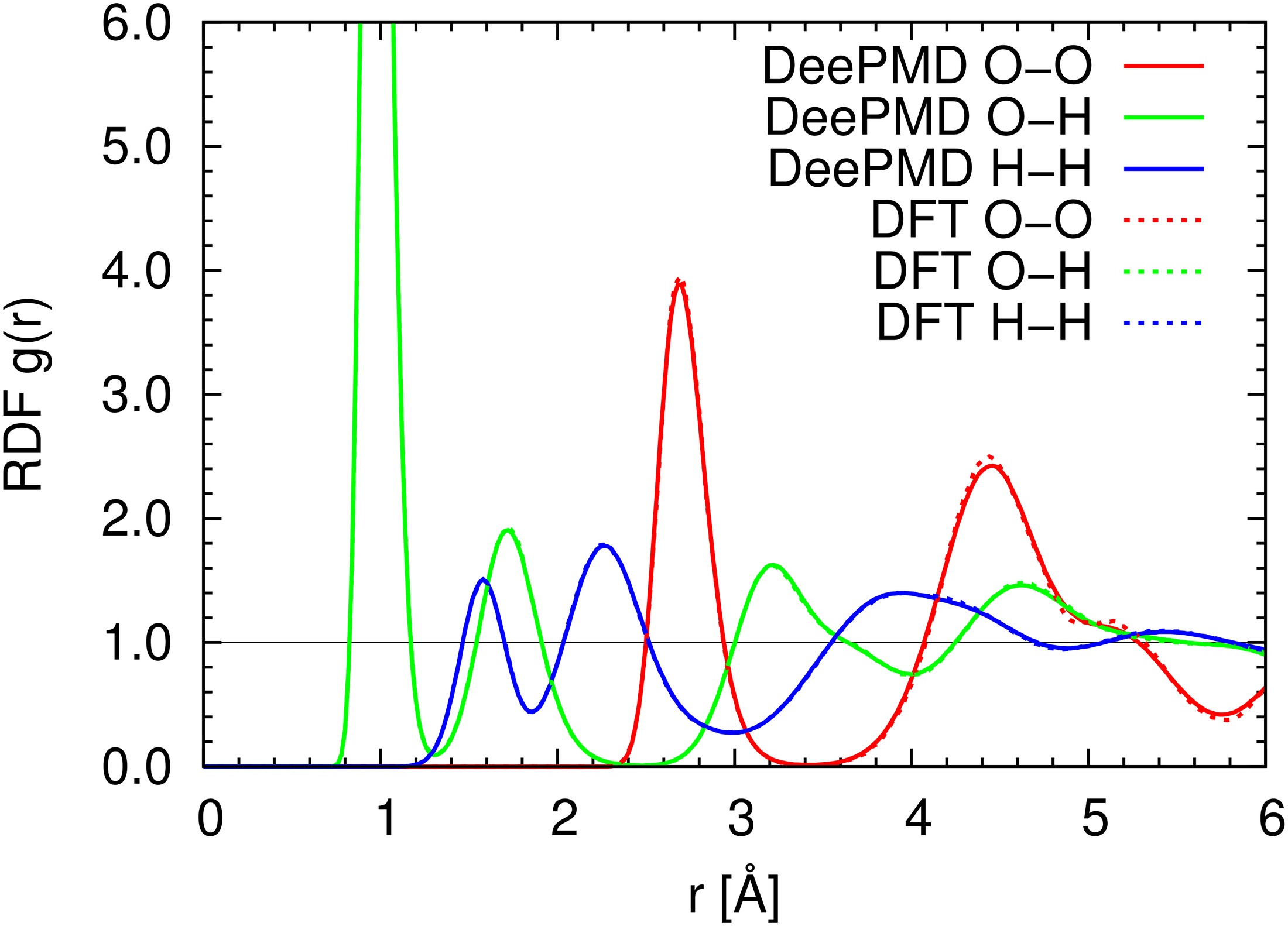
Figure 6: The comparison between the DeePMD RDFs and the AIMD RDFs of ice Ih (b).

图 6：冰 Ih (b) 的 DeePMD 径向分布函数与 AIMD 径向分布函数的比较。

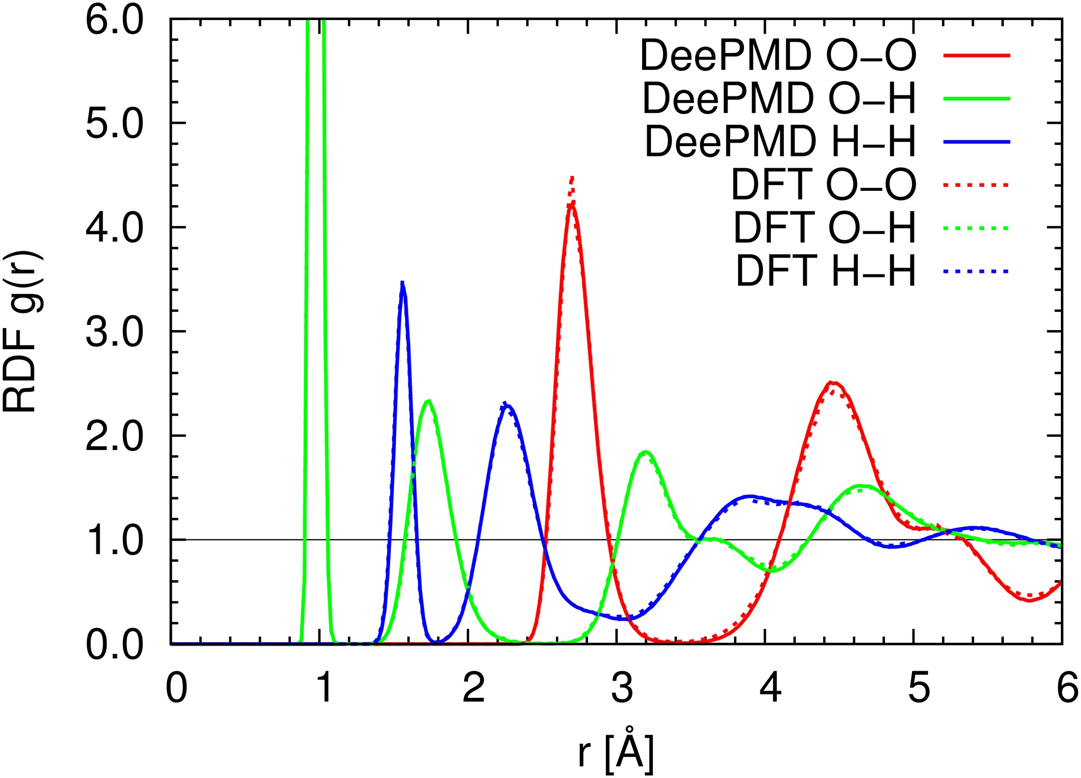
Figure 7: The comparison between the DeePMD RDFs and the AIMD RDFs of ice Ih (c).

图 7：冰 Ih (c) 的 DeePMD 径向分布函数与 AIMD 径向分布函数的比较。

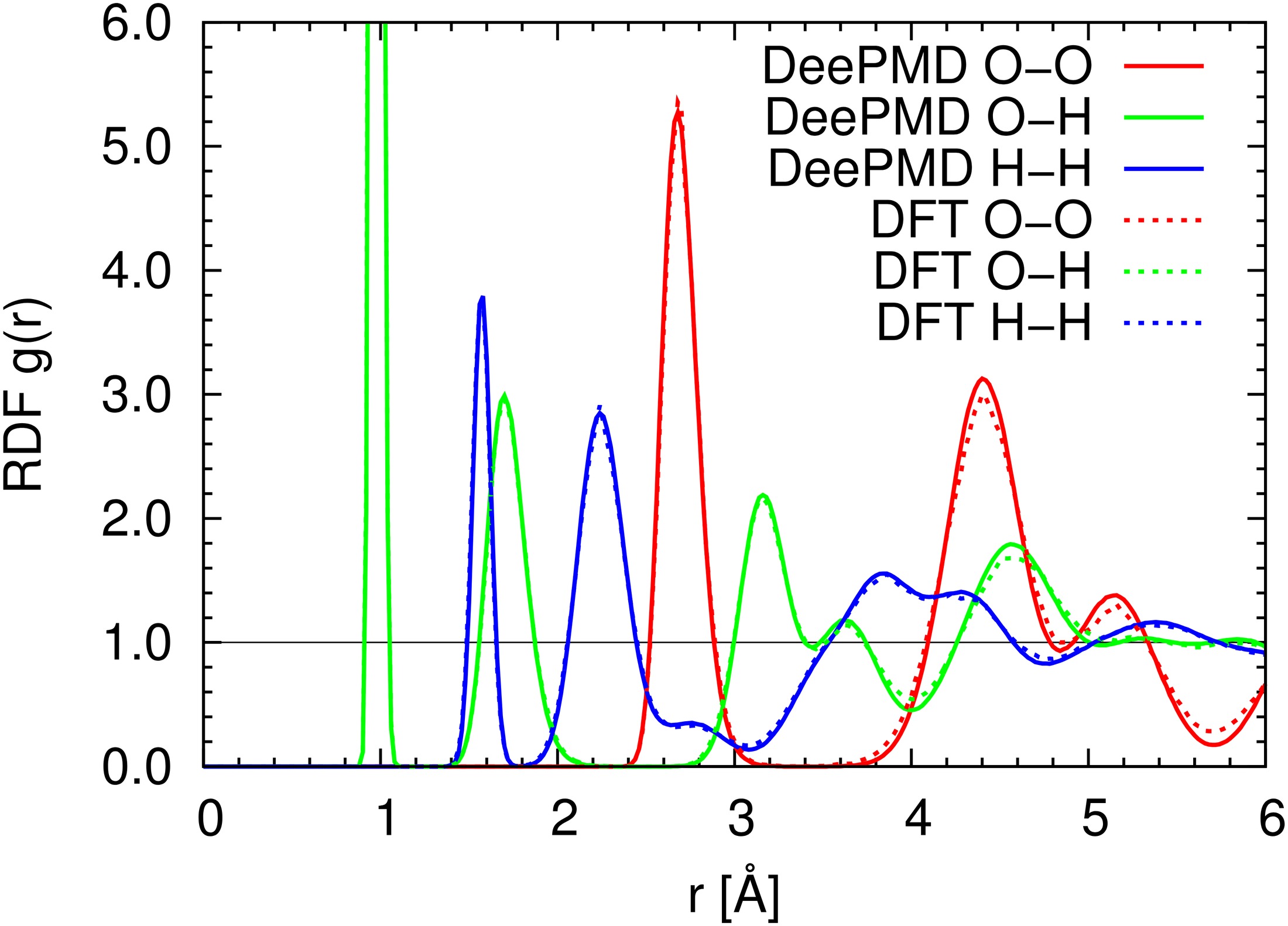
Figure 8: The comparison between the DeePMD RDFs and the AIMD RDFs of ice Ih (d).

图 8：冰 Ih (d) 的 DeePMD 径向分布函数与 AIMD 径向分布函数的比较。

The probability distribution function of the O-O bond orientation order parameter $Q_{6}$ is reported in Fig. 9. The bond orientation order parameter for oxygen $i$, as proposed in Ref. [6], is defined by

O–O 键取向序参量 $Q_{6}$ 的概率分布函数示于图 9。氧原子 $i$ 的键取向序参量按文献[6] 的提议，定义为

$$\displaystyle Q_{l}(i)=\Big[\frac{4\pi}{2l+1}\sum_{m=-l}^{l}|\bar{q}_{lm}(i)|^{2}\Big]^{\frac{1}{2}}, \tag{19}$$

where

其中

$$\displaystyle\bar{q}_{lm}(i)=\frac{\sum_{j\in\tilde{N}_{b}(i)}s(r_{ij})q_{lm}(j)}{\sum_{j\in\tilde{N}_{b}(i)}s(r_{ij})},~~q_{lm}(i)=\frac{\sum_{j\in N_{b}(i)}s(r_{ij})Y_{lm}(\hat{\textbf{{r}}}_{ij})}{\sum_{j\in N_{b}(i)}s(r_{ij})}, \tag{20}$$

and $\tilde{N}_{b}(i)=N_{b}(i)\cup\{i\}$. The $Y_{lm}(\cdots)$ denotes the spherical harmonic function, the $N_{b}(i)$ denotes the set of oxygen neighbors of oxygen $i$, and the $s(r_{ij})$ is a switching function defined by

并且 $\tilde{N}_{b}(i)=N_{b}(i)\cup\{i\}$。$Y_{lm}(\cdots)$ 表示球谐函数，$N_{b}(i)$ 表示氧原子 $i$ 的氧邻居集合，$s(r_{ij})$ 是由下式定义的开关函数

$$\displaystyle s(r)=\left{\begin{aligned} &1,&\quad&r<r_{min};\
&\frac{1}{2}+\frac{1}{2}\cos\Big(\pi,\frac{r-r_{min}}{r_{max}-r_{min}}\Big),&\quad&r_{min}\leq r<r_{max};\
&0,&\quad&r\geq r_{max}.\end{aligned}\right. \tag{21}$$

In this work we take $r_{min}=0.31$ nm and $r_{max}=0.36$ nm.

在本工作中，我们取 $r_{min}=0.31$ nm，$r_{max}=0.36$ nm。

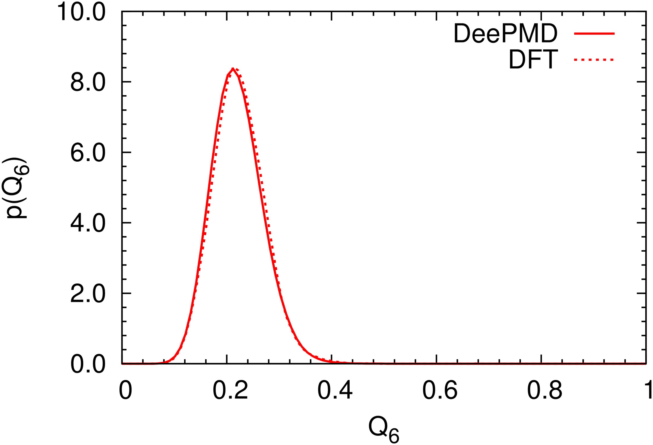
Figure 9: Probability distribution function of the O-O bond orientation order parameter $Q_{6}$

图 9：O–O 键取向序参量 $Q_{6}$ 的概率分布函数

[^4] http://www.quantum-espresso.org/

References

参考文献

[1] Ceriotti, M., Manolopoulos, D. E., and Parrinello, M., The Journal of Chemical Physics 134 , 084104 (2011).

[2] Ceriotti, M., More, J., and Manolopoulos, D. E., Computer Physics Communications 185 , 1019 (2014).

[3] Han, J., Zhang, L., Car, R., and E, W., arXiv Preprint arXiv:1707.01478 (2017).

[4] Ioffe, S. and Szegedy, C., in Proceedings of The 32nd International Conference on Machine Learning (ICML) (2015).

[5] Kingma, D. and Ba, J., in Proceedings of the International Conference on Learning Representations (ICLR) (2015).

[6] Lechner, W. and Dellago, C., The Journal of chemical physics 129 , 114707 (2008).

[7] Martyna, G. J., Klein, M. L., and Tuckerman, M., The Journal of Chemical Physics 97 , 2635 (1992).

[8] Parrinello, M. and Rahman, A., Physical Review Letters 45 , 1196 (1980).