Simple and Scalable Predictive Uncertainty Estimation using Deep Ensembles
Simple and Scalable Predictive Uncertainty Estimation using Deep Ensembles
Abstract
摘要
Deep neural networks (NNs) are powerful black box predictors that have recently achieved impressive performance on a wide spectrum of tasks. Quantifying predictive uncertainty in NNs is a challenging and yet unsolved problem. Bayesian NNs, which learn a distribution over weights, are currently the state-of-the-art for estimating predictive uncertainty; however these require significant modifications to the training procedure and are computationally expensive compared to standard (non-Bayesian) NNs. We propose an alternative to Bayesian NNs that is simple to implement, readily parallelizable, requires very little hyperparameter tuning, and yields high quality predictive uncertainty estimates. Through a series of experiments on classification and regression benchmarks, we demonstrate that our method produces well-calibrated uncertainty estimates which are as good or better than approximate Bayesian NNs. To assess robustness to dataset shift, we evaluate the predictive uncertainty on test examples from known and unknown distributions, and show that our method is able to express higher uncertainty on out-of-distribution examples. We demonstrate the scalability of our method by evaluating predictive uncertainty estimates on ImageNet.
深度神经网络(NN)是强大的黑盒预测器,近来在一系列任务上都取得了出色的表现。量化神经网络的预测不确定性,仍然是一个有挑战性、尚未解决的问题。贝叶斯神经网络通过学习权重上的分布,是当时估计预测不确定性的最先进方法;但它们需要对训练流程做显著改动,计算上也比标准(非贝叶斯)神经网络更昂贵。我们提出一种替代贝叶斯神经网络的方法,实现简单,容易并行,几乎不必调超参数,却能给出高质量的预测不确定性估计。通过在分类和回归基准上的一系列实验,我们表明该方法能产生校准良好的不确定性估计,与近似贝叶斯神经网络相当,甚至更好。为了检验对数据集偏移的稳健性,我们在来自已知和未知分布的测试样本上评估预测不确定性,并表明该方法能对分布外样本给出更高的不确定度。我们还在 ImageNet 上评估预测不确定性估计,以展示方法的可扩展性。
1 Introduction
1 引言
Deep neural networks (NNs) have achieved state-of-the-art performance on a wide variety of machine learning tasks [35] and are becoming increasingly popular in domains such as computer vision [32], speech recognition [25], natural language processing [42], and bioinformatics [2, 61]. Despite impressive accuracies in supervised learning benchmarks, NNs are poor at quantifying predictive uncertainty, and tend to produce overconfident predictions. Overconfident incorrect predictions can be harmful or offensive [3], hence proper uncertainty quantification is crucial for practical applications.
深度神经网络(NN)已在多种多样的机器学习任务上达到当时最好的表现 [35],并在计算机视觉 [32]、语音识别 [25]、自然语言处理 [42] 和生物信息学 [2, 61] 等领域越来越常见。尽管在有监督学习基准上准确率很高,神经网络却不善于量化预测不确定性,往往给出过分自信的预测。自信却错误的预测可能造成伤害或冒犯 [3],因此在实际应用中,恰当的不确定性量化至关重要。
Evaluating the quality of predictive uncertainties is challenging as the ‘ground truth’ uncertainty estimates are usually not available. In this work, we shall focus upon two evaluation measures that are motivated by practical applications of NNs. Firstly, we shall examine calibration [12, 13], a frequentist notion of uncertainty which measures the discrepancy between subjective forecasts and (empirical) long-run frequencies. The quality of calibration can be measured by proper scoring rules [17] such as log predictive probabilities and the Brier score [9]. Note that calibration is an orthogonal concern to accuracy: a network’s predictions may be accurate and yet miscalibrated, and vice versa. The second notion of quality of predictive uncertainty we consider concerns generalization of the predictive uncertainty to domain shift (also referred to as out-of-distribution examples [23]), that is, measuring if the network knows what it knows. For example, if a network trained on one dataset is evaluated on a completely different dataset, then the network should output high predictive uncertainty as inputs from a different dataset would be far away from the training data. Well-calibrated predictions that are robust to model misspecification and dataset shift have a number of important practical uses (e.g., weather forecasting, medical diagnosis).
评估预测不确定性的质量并不容易,因为通常并没有“真实”的不确定性估计可供对照。本文关注由神经网络实际应用所引出的两项评估指标。第一项是校准 [12, 13],这是一种频率学派的不确定性概念,用来衡量主观预报与(经验的)长期频率之间的差距。校准的好坏可以用适当评分规则 [17] 来度量,例如对数预测概率和 Brier 分数 [9]。需要注意,校准与准确率是正交的:网络的预测可以很准却校准不良,反过来也可以。我们考虑的第二项质量,是预测不确定性对域偏移(也称分布外样本 [23])的泛化,也就是衡量网络是否知道自己知道什么。例如,若在一个数据集上训练的网络被放到完全不同的数据集上评估,它应当输出很高的预测不确定度,因为来自另一数据集的输入会远离训练数据。对模型误设和数据集偏移都稳健的、校准良好的预测,有许多重要的实际用途(例如天气预报、医学诊断)。
31st Conference on Neural Information Processing Systems (NIPS 2017), Long Beach, CA, USA.
第 31 届神经信息处理系统大会(NIPS 2017),美国加利福尼亚州长滩。
There has been a lot of recent interest in adapting NNs to encompass uncertainty and probabilistic methods. The majority of this work revolves around a Bayesian formalism [4], whereby a prior distribution is specified upon the parameters of a NN and then, given the training data, the posterior distribution over the parameters is computed, which is used to quantify predictive uncertainty. Since exact Bayesian inference is computationally intractable for NNs, a variety of approximations have been developed including Laplace approximation [40], Markov chain Monte Carlo (MCMC) methods [46], as well as recent work on variational Bayesian methods [6, 19, 39], assumed density filtering [24], expectation propagation [21, 38] and stochastic gradient MCMC variants such as Langevin diffusion methods [30, 59] and Hamiltonian methods [53]. The quality of predictive uncertainty obtained using Bayesian NNs crucially depends on (i) the degree of approximation due to computational constraints and (ii) if the prior distribution is ‘correct’, as priors of convenience can lead to unreasonable predictive uncertainties [50]. In practice, Bayesian NNs are often harder to implement and computationally slower to train compared to non-Bayesian NNs, which raises the need for a ‘general purpose solution’ that can deliver high-quality uncertainty estimates and yet requires only minor modifications to the standard training pipeline.
近来有不少工作希望把不确定性与概率方法引入神经网络。其中大部分围绕贝叶斯形式 [4]:先为网络参数指定先验分布,再根据训练数据计算参数的后验,并用此后验来量化预测不确定性。由于精确贝叶斯推断对神经网络在计算上不可行,人们发展了多种近似,包括拉普拉斯近似 [40]、马尔可夫链蒙特卡洛(MCMC)方法 [46],以及近期的变分贝叶斯方法 [6, 19, 39]、假定密度滤波 [24]、期望传播 [21, 38],还有随机梯度 MCMC 的变体,例如 Langevin 扩散方法 [30, 59] 和哈密顿方法 [53]。用贝叶斯神经网络得到的预测不确定性,其质量关键取决于(i)受计算约束所做近似的程度,以及(ii)先验分布是否“正确”,因为图方便而取的先验可能导致不合理的预测不确定性 [50]。实践中,贝叶斯神经网络往往比非贝叶斯网络更难实现,训练也更慢,因而需要一种“通用解法”:既能给出高质量的不确定性估计,又只需对标准训练流程做很小的改动。
Recently, Gal and Ghahramani [15] proposed using Monte Carlo dropout (MC-dropout) to estimate predictive uncertainty by using Dropout [54] at test time. There has been work on approximate Bayesian interpretation [15, 29, 41] of dropout. MC-dropout is relatively simple to implement leading to its popularity in practice. Interestingly, dropout may also be interpreted as ensemble model combination [54] where the predictions are averaged over an ensemble of NNs (with parameter sharing). The ensemble interpretation seems more plausible particularly in the scenario where the dropout rates are not tuned based on the training data, since any sensible approximation to the true Bayesian posterior distribution has to depend on the training data. This interpretation motivates the investigation of ensembles as an alternative solution for estimating predictive uncertainty.
近来,Gal 和 Ghahramani [15] 提出用蒙特卡洛 Dropout(MC-dropout),在测试时使用 Dropout [54] 来估计预测不确定性。也有工作讨论 Dropout 的近似贝叶斯解释 [15, 29, 41]。MC-dropout 实现相对简单,因而在实践中很流行。有意思的是,Dropout 也可以解释成集成模型组合 [54],也就是在一组(共享参数的)神经网络上平均预测。在 Dropout 率并不根据训练数据来调节的情形下,这种集成解释显得更合理,因为对真实贝叶斯后验的任何像样近似,都应当依赖于训练数据。这一解释促使我们把集成当作估计预测不确定性的另一条路来考察。
It has long been observed that ensembles of models improve predictive performance (see [14] for a review). However it is not obvious when and why an ensemble of NNs can be expected to produce good uncertainty estimates. Bayesian model averaging (BMA) assumes that the true model lies within the hypothesis class of the prior, and performs soft model selection to find the single best model within the hypothesis class [43]. In contrast, ensembles perform model combination, i.e. they combine the models to obtain a more powerful model; ensembles can be expected to be better when the true model does not lie within the hypothesis class. We refer to [11, 43] and [34, §2.5] for related discussions. It is important to note that even exact BMA is not guaranteed be robust to mis-specification with respect to domain shift.
人们很早就观察到,模型集成能提高预测表现(综述见 [14])。但何时、为何一组神经网络的集成能够给出好的不确定性估计,并不显然。贝叶斯模型平均(BMA)假定真实模型落在先验的假设类之内,并做软模型选择,以在假设类中找到单个最好的模型 [43]。相比之下,集成做的是模型组合,也就是把多个模型合起来得到更强的模型;当真实模型并不落在假设类之内时,集成有望更好。相关讨论见 [11, 43] 以及 [34, §2.5]。需要指出,即便是精确的 BMA,也不能保证对域偏移下的误设保持稳健。
Summary of contributions: Our contribution in this paper is two fold. First, we describe a simple and scalable method for estimating predictive uncertainty estimates from NNs. We argue for training probabilistic NNs (that model predictive distributions) using a proper scoring rule as the training criteria. We additionally investigate the effect of two modifications to the training pipeline, namely (i) ensembles and (ii) adversarial training [18] and describe how they can produce smooth predictive estimates. Secondly, we propose a series of tasks for evaluating the quality of the predictive uncertainty estimates, in terms of calibration and generalization to unknown classes in supervised learning problems. We show that our method significantly outperforms (or matches) MC-dropout. These tasks, along with our simple yet strong baseline, serve as an useful benchmark for comparing predictive uncertainty estimates obtained using different Bayesian/non-Bayesian/hybrid methods.
贡献摘要:本文的贡献有两方面。第一,我们描述一种简单、可扩展的方法,用来从神经网络得到预测不确定性估计。我们主张用适当评分规则作为训练准则,去训练对预测分布建模的概率神经网络。我们还考察对训练流程的两处改动,即(i)集成和(ii)对抗训练 [18],并说明它们如何能够给出平滑的预测估计。第二,我们提出一系列任务,从校准以及有监督学习中对未知类别的泛化出发,评估预测不确定性估计的质量。我们表明,该方法显著优于(或与之相当)MC-dropout。这些任务,连同我们简单却很强的基线,可以作为比较不同贝叶斯 / 非贝叶斯 / 混合方法所得预测不确定性估计的有用基准。
Novelty and Significance: Ensembles of NNs, or deep ensembles for short, have been successfully used to boost predictive performance (e.g. classification accuracy in ImageNet or Kaggle contests) and adversarial training has been used to improve robustness to adversarial examples. However, to the best of our knowledge, ours is the first work to investigate their usefulness for predictive uncertainty estimation and compare their performance to current state-of-the-art approximate Bayesian methods on a series of classification and regression benchmark datasets. Compared to Bayesian NNs (e.g. variational inference or MCMC methods), our method is much simpler to implement, requires surprisingly few modifications to standard NNs, and well suited for distributed computation, thereby making it attractive for large-scale deep learning applications. To demonstrate scalability of our method, we evaluate predictive uncertainty on ImageNet (and are the first to do so, to the best of our knowledge). Most work on uncertainty in deep learning focuses on Bayesian deep learning; we hope that the simplicity and strong empirical performance of our approach will spark more interest in non-Bayesian approaches for predictive uncertainty estimation.
新颖性与意义:神经网络的集成,简称深度集成,已被成功用来提升预测表现(例如 ImageNet 或 Kaggle 竞赛中的分类准确率),对抗训练则被用来提高对对抗样本的稳健性。但据我们所知,本文是第一项考察它们对预测不确定性估计是否有用,并在一系列分类和回归基准数据集上,把它们的表现与当时最先进的近似贝叶斯方法相比较的工作。与贝叶斯神经网络(例如变分推断或 MCMC 方法)相比,我们的方法实现简单得多,对标准神经网络的改动出奇地少,也适合分布式计算,因而对大规模深度学习应用很有吸引力。为展示可扩展性,我们在 ImageNet 上评估了预测不确定性(据我们所知也是第一次这样做)。深度学习中大多数关于不确定性的工作都聚焦于贝叶斯深度学习;我们希望这一方法的简单性与很强的经验表现,能引起人们对非贝叶斯预测不确定性估计方法的更多兴趣。
2 Deep Ensembles: A Simple Recipe For Predictive Uncertainty Estimation
2 深度集成:估计预测不确定性的简单做法
2.1 Problem setup and High-level summary
2.1 问题设定与概要
We assume that the training dataset consists of i.i.d. data points , where represents the -dimensional features. For classification problems, the label is assumed to be one of classes, that is . For regression problems, the label is assumed to be real-valued, that is . Given the input features , we use a neural network to model the probabilistic predictive distribution over the labels, where are the parameters of the NN.
假定训练数据集 由 个独立同分布的数据点组成,,其中 表示 维特征。对分类问题,标签假定是 类之一,即 。对回归问题,标签假定是实值,即 。给定输入特征 ,我们用神经网络对标签上的概率预测分布 建模,其中 是网络参数。
We suggest a simple recipe: (1) use a proper scoring rule as the training criterion, (2) use adversarial training [18] to smooth the predictive distributions, and (3) train an ensemble. Let denote the number of NNs in the ensemble and denote the parameters of the ensemble. We first describe how to train a single neural net and then explain how to train an ensemble of NNs.
我们给出一个简单做法:(1)用适当评分规则作为训练准则,(2)用对抗训练 [18] 来平滑预测分布,(3)训练一个集成。记 为集成中神经网络的数目, 为集成的参数。我们先说明如何训练单个网络,再说明如何训练一组网络。
2.2 Proper scoring rules
2.2 适当评分规则
Scoring rules measure the quality of predictive uncertainty (see [17] for a review). A scoring rule assigns a numerical score to a predictive distribution , rewarding better calibrated predictions over worse. We shall consider scoring rules where a higher numerical score is better. Let a scoring rule be a function that evaluates the quality of the predictive distribution relative to an event where denotes the true distribution on -tuples. The expected scoring rule is then . A proper scoring rule is one where with equality if and only if , for all and . NNs can then be trained according to measure that encourages calibration of predictive uncertainty by minimizing the loss .
评分规则用来衡量预测不确定性的质量(综述见 [17])。评分规则给预测分布 赋一个数值分数,校准更好的预测得到更高的奖励。我们考虑分数越高越好的评分规则。设评分规则是函数 ,它相对于事件 来评估预测分布 的质量,其中 表示 对上的真实分布。期望评分规则于是是 。适当评分规则满足 ,当且仅当 时等号成立,对所有 和 都如此。于是可以通过最小化损失 ,按这一鼓励预测不确定性校准的度量来训练神经网络。
It turns out many common NN loss functions are proper scoring rules. For example, when maximizing likelihood, the score function is , and this is a proper scoring rule due to Gibbs inequality: . In the case of multi-class -way classification, the popular softmax cross entropy loss is equivalent to the log likelihood and is a proper scoring rule. Interestingly, , i.e., minimizing the squared error between the predictive probability of a label and one-hot encoding of the correct label, is also a proper scoring rule known as the Brier score [9]. This provides justification for this common trick for training NNs by minimizing the squared error between a binary label and its associated probability and shows it is, in fact, a well defined loss with desirable properties.(^1)
其实许多常见的神经网络损失函数本身就是适当评分规则。例如在极大似然时,评分函数是 ,由 Gibbs 不等式可知这是适当评分规则:。在多类 路分类中,常用的 softmax 交叉熵损失等价于对数似然,因而也是适当评分规则。有意思的是,,也就是最小化标签预测概率与正确标签独热编码之间的平方误差,同样是一种适当评分规则,称为 Brier 分数 [9]。这为用平方误差来训练神经网络、最小化二值标签与其对应概率之差这一常见技巧提供了依据,并表明它其实是一种定义良好、性质可取的损失。(^1)
Indeed as noted in Gneiting and Raftery [17], it can be shown that asymptotically maximizing any proper scoring rule recovers true parameter values.
正如 Gneiting 和 Raftery [17] 所指出的,可以证明,渐近地最大化任一适当评分规则,都能恢复真实参数值。
2.2.1 Training criterion for regression
2.2.1 回归的训练准则
For regression problems, NNs usually output a single value say and the parameters are optimized to minimize the mean squared error (MSE) on the training set, given by . However, the MSE does not capture predictive uncertainty. Following [47], we use a network that outputs two values in the final layer, corresponding to the predicted mean and variance(^2) . By treating the observed value as a sample from a (heteroscedastic) Gaussian distribution with the predicted mean and variance, we minimize the negative log-likelihood criterion:
对回归问题,神经网络通常只输出一个值,记为 ,参数则按训练集上的均方误差(MSE)来优化,即 。但均方误差并不能刻画预测不确定性。遵循 [47],我们使用在最后一层输出两个值的网络,分别对应预测均值 和方差(^2) 。把观测值视为来自以该预测均值和方差为参数的(异方差)高斯分布的样本,我们最小化负对数似然准则:
We enforce the positivity constraint on the variance by passing the second output through the softplus function , and add a minimum variance (e.g. ) for numerical stability.
我们把第二个输出经 softplus 函数 再输出,以施加方差的正性约束,并加上一个最小方差(例如 )以保证数值稳定。
We found the above to perform satisfactorily in our experiments. However, two simple extensions are worth further investigation: (i) Maximum likelihood estimation over and might overfit; one could impose a prior and perform maximum-a-posteriori (MAP) estimation. (ii) In cases where the Gaussian is too-restrictive, one could use a complex distribution e.g. mixture density network [5] or a heavy-tailed distribution.
我们发现上述做法在实验中表现令人满意。不过有两个简单的扩展值得进一步研究:(i)对 和 做极大似然估计可能会过拟合;可以施加先验并做最大后验(MAP)估计。(ii)在高斯分布过于受限的情形下,可以使用更复杂的分布,例如混合密度网络 [5],或重尾分布。
2.3 Adversarial training to smooth predictive distributions
2.3 用对抗训练平滑预测分布
Adversarial examples, proposed by Szegedy et al. [55] and extended by Goodfellow et al. [18], are those which are ‘close’ to the original training examples (e.g. an image that is visually indistinguishable from the original image to humans), but are misclassified by the NN. Goodfellow et al. [18] proposed the fast gradient sign method as a fast solution to generate adversarial examples. Given an input with target , and loss (e.g. ), the fast gradient sign method generates an adversarial example as , where is a small value such that the max-norm of the perturbation is bounded. Intuitively, the adversarial perturbation creates a new training example by adding a perturbation along a direction which the network is likely to increase the loss. Assuming is small enough, these adversarial examples can be used to augment the original training set by treating as additional training examples. This procedure, referred to as adversarial training,(^3) was found to improve the classifier’s robustness [18].
对抗样本由 Szegedy 等人 [55] 提出,并由 Goodfellow 等人 [18] 推广,指的是与原始训练样本“接近”(例如对人眼来说与原图几乎无法区分的图像),却会被神经网络分错的样本。Goodfellow 等人 [18] 提出快速梯度符号法,作为快速生成对抗样本的办法。给定输入 、目标 以及损失 (例如 ),快速梯度符号法生成对抗样本 ,其中 是一个很小的值,使得扰动的最大范数有界。直观上,对抗扰动沿着网络很可能增大损失的方向加上一个扰动,从而造出一个新的训练样本。只要 足够小,就可以把 当作额外训练样本,用来扩充原来的训练集。这一做法称为对抗训练(^3),被发现能够提高分类器的稳健性 [18]。
Not to be confused with Generative Adversarial Networks (GANs).
不要与生成对抗网络(GAN)混淆。
Interestingly, adversarial training can be interpreted as a computationally efficient solution to smooth the predictive distributions by increasing the likelihood of the target around an -neighborhood of the observed training examples. Ideally one would want to smooth the predictive distributions along all directions in ; however this is computationally expensive. A random direction might not necessarily increase the loss; however, adversarial training by definition computes the direction where the loss is high and hence is better than a random direction for smoothing predictive distributions. Miyato et al. [44] proposed a related idea called virtual adversarial training (VAT), where they picked ; the advantage of VAT is that it does not require knowledge of the true target and hence can be applied to semi-supervised learning. Miyato et al. [44] showed that distributional smoothing using VAT is beneficial for efficient semi-supervised learning; in contrast, we investigate the use of adversarial training for predictive uncertainty estimation. Hence, our contributions are complementary; one could use VAT or other forms of adversarial training, cf. [33], for improving predictive uncertainty in the semi-supervised setting as well.
有意思的是,对抗训练可以理解为一种计算上高效的办法,通过提高观测训练样本 -邻域内目标的似然,来平滑预测分布。理想情形下,人们希望沿 中全部 个方向去平滑预测分布;但这在计算上很贵。随机方向不一定会增大损失;而对抗训练按定义计算的是损失高的方向,因而比随机方向更适合用来平滑预测分布。Miyato 等人 [44] 提出了一种相关想法,称为虚拟对抗训练(VAT),他们取 ;VAT 的优点是不必知道真实目标 ,因而可以用于半监督学习。Miyato 等人 [44] 表明,用 VAT 做分布平滑有利于高效的半监督学习;相比之下,我们考察的是把对抗训练用于预测不确定性估计。因此,双方的贡献是互补的;在半监督设定下,也可以用 VAT 或其他形式的对抗训练,参见 [33],来改进预测不确定性。
2.4 Ensembles: training and prediction
2.4 集成:训练与预测
The most popular ensembles use decision trees as the base learners and a wide variety of method have been explored in the literature on ensembles. Broadly, there are two classes of ensembles: randomization-based approaches such as random forests [8], where the ensemble members can be trained in parallel without any interaction, and boosting-based approaches where the ensemble members are fit sequentially. We focus only on the randomization based approach as it is better suited for distributed, parallel computation. Breiman [8] showed that the generalization error of random forests can be upper bounded by a function of the strength and correlation between individual trees; hence it is desirable to use a randomization scheme that de-correlates the predictions of the individual models as well as ensures that the individual models are strong (e.g. high accuracy). One of the popular strategies is bagging (a.k.a. bootstrapping), where ensemble members are trained on different bootstrap samples of the original training set. If the base learner lacks intrinsic randomization (e.g. it can be trained efficiently by solving a convex optimization problem), bagging is a good mechanism for inducing diversity. However, if the underlying base learner has multiple local optima, as is the case typically with NNs, the bootstrap can sometimes hurt performance since a base learner trained on a bootstrap sample sees only 63% unique data points.(^4)
最常见的集成以决策树作为基学习器,集成方面的文献也探索了多种多样的方法。大致说来,集成有两类:一类是基于随机化的方法,例如随机森林 [8],其中各成员可以互不交互地并行训练;另一类是基于提升的方法,成员被依次拟合。我们只关注基于随机化的方法,因为它更适合分布式、并行计算。Breiman [8] 表明,随机森林的泛化误差可以被单个树的强度及其相关性的一个函数上界住;因此,理想的随机化方案既要降低各模型预测之间的相关性,又要保证单个模型足够强(例如准确率高)。一种常用策略是装袋(又称自助法),各成员在原始训练集的不同自助样本上训练。如果基学习器本身缺乏内在随机性(例如可以通过求解凸优化问题高效训练),装袋是引入多样性的好机制。然而,若基学习器有多个局部最优——神经网络通常如此——自助法有时反而会损害表现,因为在自助样本上训练的基学习器只看到约 63% 的不重复数据点。(^4)
The bootstrap draws times uniformly with replacement from a dataset with items. The probability an item is picked at least once is , which for large becomes . Hence, the number of unique data points in a bootstrap sample is on average.
自助法从一个含 个条目的数据集中有放回地均匀抽取 次。某个条目至少被抽到一次的概率是 ,当 很大时变为 。因此,一个自助样本中不重复数据点的数目平均为 。
In the literature on decision tree ensembles, Breiman [8] proposed to use a combination of bagging [7] and random subset selection of features at each node. Geurts et al. [16] later showed that bagging is unnecessary if additional randomness can be injected into the random subset selection procedure. Intuitively, using more data for training the base learners helps reduce their bias and ensembling helps reduce the variance.
在决策树集成的文献中,Breiman [8] 提出把装袋 [7] 与在每个节点上随机选取特征子集结合起来。Geurts 等人 [16] 后来表明,如果能在随机子集选择过程中注入额外的随机性,装袋就不再必要。直观上,用更多数据训练基学习器有助于降低其偏差,而集成有助于降低方差。
We used the entire training dataset to train each network since deep NNs typically perform better with more data, although it is straightforward to use a random subsample if need be. We found that random initialization of the NN parameters, along with random shuffling of the data points, was sufficient to obtain good performance in practice. We observed that bagging deteriorated performance in our experiments. Lee et al. [36] independently observed that training on entire dataset with random initialization was better than bagging for deep ensembles, however their goal was to improve predictive accuracy and not predictive uncertainty. The overall training procedure is summarized in Algorithm 1.
我们用整个训练集来训练每一个网络,因为深度神经网络通常在数据更多时表现更好;当然,若有需要,改用随机子样本也很直接。我们发现,对网络参数做随机初始化,再加上对数据点做随机打乱,在实践中就足以获得良好表现。我们观察到,装袋在实验中反而降低了表现。Lee 等人 [36] 也独立观察到,对深度集成而言,用整个数据集加随机初始化来训练,要优于装袋,不过他们的目标是提高预测准确率,而不是预测不确定性。整体训练流程总结在算法 1 中。
Algorithm 1 Pseudocode of the training procedure for our method
- Let each neural network parametrize a distribution over the outputs, i.e. . Use a proper scoring rule as the training criterion . Recommended default values are and of the input range of the corresponding dimension (e.g 2.55 if input range is ).
- Initialize randomly.
- for do (train networks independently in parallel)
- Sample data point randomly for each net (single for clarity, minibatch in practice).
- Generate adversarial example using x\'_{n_m}=x_{n_m}+\epsilon\,\mathrm{sign}(\nabla_{x_{n_m}}\ell(\theta_m,x_{n_m},y_{n_m})).
- Minimize \ell(\theta_m,x_{n_m},y_{n_m})+\ell(\theta_m,x\'_{n_m},y_{n_m}) w.r.t. . (adversarial training, optional)
算法 1 本文方法训练流程的伪代码
- 让每个神经网络对输出上的分布参数化,即 。用适当评分规则作为训练准则 。推荐的默认值是 ,以及 取相应维输入范围的 (例如输入范围为 时取 2.55)。
- 随机初始化 。
- for do(各网络独立并行训练)
- 为每个网络随机抽取数据点 (为清楚起见写成单个 ,实践中用小批量)。
- 生成对抗样本 x\'_{n_m}=x_{n_m}+\epsilon\,\mathrm{sign}(\nabla_{x_{n_m}}\ell(\theta_m,x_{n_m},y_{n_m}))。
- 关于 最小化 \ell(\theta_m,x_{n_m},y_{n_m})+\ell(\theta_m,x\'_{n_m},y_{n_m})。(对抗训练,可选)
We treat the ensemble as a uniformly-weighted mixture model and combine the predictions as . For classification, this corresponds to averaging the predicted probabilities. For regression, the prediction is a mixture of Gaussian distributions. For ease of computing quantiles and predictive probabilities, we further approximate the ensemble prediction as a Gaussian whose mean and variance are respectively the mean and variance of the mixture. The mean and variance of a mixture are given by and respectively.
我们把集成当作均匀加权的混合模型,并把预测组合为 。对分类,这对应于对预测概率取平均。对回归,预测是若干高斯分布的混合。为便于计算分位数和预测概率,我们进一步把集成预测近似成一个高斯,其均值和方差分别取该混合的均值和方差。混合 的均值和方差分别由 和 给出。
3 Experimental results
3 实验结果
3.1 Evaluation metrics and experimental setup
3.1 评估指标与实验设定
For both classification and regression, we evaluate the negative log likelihood (NLL) which depends on the predictive uncertainty. NLL is a proper scoring rule and a popular metric for evaluating predictive uncertainty [49]. For classification we additionally measure classification accuracy and the Brier score, defined as where if , and otherwise. For regression problems, we additionally measured the root mean squared error (RMSE). Unless otherwise specified, we used batch size of 100 and Adam optimizer with fixed learning rate of 0.1 in our experiments. We use the same technique for generating adversarial training examples for regression problems. Goodfellow et al. [18] used a fixed for all dimensions; this is unsatisfying if the input dimensions have different ranges. Hence, in all of our experiments, we set to 0.01 times the range of the training data along that particular dimension. We used the default weight initialization in Torch.
对分类和回归,我们都评估依赖于预测不确定性的负对数似然(NLL)。NLL 是适当评分规则,也是评估预测不确定性的常用指标 [49]。对分类,我们还测量分类准确率以及 Brier 分数,定义为 ,其中若 则 ,否则为 。对回归问题,我们还测量均方根误差(RMSE)。除非另有说明,实验中批量大小取 100,优化器用 Adam,学习率固定为 0.1。回归问题上,我们用同样的办法生成对抗训练样本。Goodfellow 等人 [18] 对所有维使用固定的 ;若各输入维的范围不同,这就不合适。因此在全部实验中,我们把 设为该维训练数据范围的 0.01 倍。权重初始化采用 Torch 的默认方式。
3.2 Regression on toy datasets
3.2 玩具数据集上的回归
First, we qualitatively evaluate the performance of the proposed method on a one-dimensional toy regression dataset. This dataset was used by Hernández-Lobato and Adams [24], and consists of 20 training examples drawn as where . We used the same architecture as [24].
首先,我们在一个一维玩具回归数据集上定性评估所提方法的表现。该数据集由 Hernández-Lobato 和 Adams [24] 使用,包含 20 个按 抽取的训练样本,其中 。网络结构与 [24] 相同。
A commonly used heuristic in practice is to use an ensemble of NNs (trained to minimize MSE), obtain multiple point predictions and use the empirical variance of the networks’ predictions as an approximate measure of uncertainty. We demonstrate that this is inferior to learning the variance by training using NLL.(^5) The results are shown in Figure 1.
实践中一种常用启发式是:用一组(按均方误差训练的)神经网络,得到多个点预测,再把各网络预测的经验方差当作不确定性的近似度量。我们表明,这不如通过用 NLL 训练来学习方差。(^5) 结果见图 1。
See also Appendix A.2 for calibration results on a real world dataset.
真实数据集上的校准结果亦见附录 A.2。
 \n\nFigure 1: Results on a toy regression task: -axis denotes . On the -axis, the blue line is the ground truth curve, the red dots are observed noisy training data points and the gray lines correspond to the predicted mean along with three standard deviations. Left most plot corresponds to empirical variance of 5 networks trained using MSE, second plot shows the effect of training using NLL using a single net, third plot shows the additional effect of adversarial training, and final plot shows the effect of using an ensemble of 5 networks respectively.
图 1:玩具回归任务上的结果:横轴表示 。纵轴上,蓝线是真实曲线,红点是观测到的带噪声训练数据点,灰线对应预测均值以及三倍标准差。最左图对应用均方误差训练的 5 个网络的经验方差,第二图给出用 NLL 训练单个网络的效果,第三图给出再加上对抗训练的效果,最后一图给出使用 5 个网络组成的集成的效果。
The results clearly demonstrate that (i) learning variance and training using a scoring rule (NLL) leads to improved predictive uncertainty and (ii) ensemble combination improves performance, especially as we move farther from the observed training data.
结果清楚地表明:(i)学习方差并用评分规则(NLL)训练,能改进预测不确定性;(ii)集成组合能提高表现,尤其是当我们远离已观测的训练数据时。
3.3 Regression on real world datasets
3.3 真实世界数据集上的回归
In our next experiment, we compare our method to state-of-the-art methods for predictive uncertainty estimation using NNs on regression tasks. We use the experimental setup proposed by Hernández-Lobato and Adams [24] for evaluating probabilistic backpropagation (PBP), which was also used by Gal and Ghahramani [15] to evaluate MC-dropout.(^6) Each dataset is split into 20 train-test folds, except for the protein dataset which uses 5 folds and the Year Prediction MSD dataset which uses a single train-test split. We use the identical network architecture: 1-hidden layer NN with ReLU nonlinearity [45], containing 50 hidden units for smaller datasets and 100 hidden units for the larger protein and Year Prediction MSD datasets. We trained for 40 epochs; we refer to [24] for further details about the datasets and the experimental protocol. We used 5 networks in our ensemble. Our results are shown in Table 1, along with the PBP and MC-dropout results reported in their respective papers.
在下一个实验中,我们在回归任务上把该方法与用神经网络估计预测不确定性的当时最先进方法相比较。我们采用 Hernández-Lobato 和 Adams [24] 为评估概率反向传播(PBP)提出的实验设定,Gal 和 Ghahramani [15] 评估 MC-dropout 时也使用了这一设定。(^6) 每个数据集都被分成 20 个训练–测试折,蛋白数据集除外(使用 5 折),Year Prediction MSD 数据集则只用一次训练–测试划分。网络结构完全相同:单隐层、带 ReLU 非线性 [45] 的神经网络,较小数据集用 50 个隐单元,较大的蛋白和 Year Prediction MSD 数据集用 100 个隐单元。我们训练 40 个周期;数据集和实验协议的更多细节见 [24]。集成中使用 5 个网络。结果见表 1,并附上各自论文中报告的 PBP 和 MC-dropout 结果。
We do not compare to VI [19] as PBP and MC-dropout outperform VI on these benchmarks.
我们不与变分推断(VI)[19] 比较,因为在这些基准上 PBP 和 MC-dropout 已优于 VI。
Table 1: Results on regression benchmark datasets comparing RMSE and NLL. See Table 2 for results on variants of our method.
| Datasets | RMSE | NLL | ||||
|---|---|---|---|---|---|---|
| PBP | MC-dropout | Deep Ensembles | PBP | MC-dropout | Deep Ensembles | |
| Boston housing | ||||||
| Concrete | ||||||
| Energy | ||||||
| Kin8nm | ||||||
| Naval propulsion plant | ||||||
| Power plant | ||||||
| Protein | ||||||
| Wine | ||||||
| Yacht | ||||||
| Year Prediction MSD |
表 1:回归基准数据集上比较 RMSE 与 NLL 的结果。本文方法各变体的结果见表 2。
| 数据集 | RMSE | NLL | ||||
|---|---|---|---|---|---|---|
| PBP | MC-dropout | Deep Ensembles | PBP | MC-dropout | Deep Ensembles | |
| Boston housing | ||||||
| Concrete | ||||||
| Energy | ||||||
| Kin8nm | ||||||
| Naval propulsion plant | ||||||
| Power plant | ||||||
| Protein | ||||||
| Wine | ||||||
| Yacht | ||||||
| Year Prediction MSD |
We observe that our method outperforms (or is competitive with) existing methods in terms of NLL. On some datasets, we observe that our method is slightly worse in terms of RMSE. We believe that this is due to the fact that our method optimizes for NLL (which captures predictive uncertainty) instead of MSE. Table 2 in Appendix A.1 reports additional results on variants of our method, demonstrating the advantage of using an ensemble as well as learning variance.
我们观察到,就 NLL 而言,该方法优于(或至少不差于)现有方法。在部分数据集上,就 RMSE 而言略差。我们认为这是因为该方法优化的是捕捉预测不确定性的 NLL,而不是均方误差。附录 A.1 中的表 2 报告了本文方法各变体的额外结果,说明了使用集成以及学习方差的好处。
3.4 Classification on MNIST, SVHN and ImageNet
3.4 MNIST、SVHN 与 ImageNet 上的分类
Next we evaluate the performance on classification tasks using MNIST and SVHN datasets. Our goal is not to achieve the state-of-the-art performance on these problems, but rather to evaluate the effect of adversarial training as well as the number of networks in the ensemble. To verify if adversarial training helps, we also include a baseline which picks a random signed vector.
接下来,我们在 MNIST 和 SVHN 数据集的分类任务上评估表现。我们的目标并不是在这些问题上达到当时最先进的水平,而是评估对抗训练以及集成中网络个数的效果。为了检验对抗训练是否有帮助,我们还加入了一个选取随机符号向量的基线。
For MNIST, we used an MLP with 3-hidden layers with 200 hidden units per layer and ReLU non-linearities with batch normalization. For MC-dropout, we added dropout after each non-linearity with 0.1 as the dropout rate.(^7) Results are shown in Figure 2(a). We observe that adversarial training and increasing the number of networks in the ensemble significantly improve performance in terms of both classification accuracy as well as NLL and Brier score, illustrating that our method produces well-calibrated uncertainty estimates. Adversarial training leads to better performance than augmenting with random direction. Our method also performs much better than MC-dropout in terms of all the performance measures. Note that augmenting the training dataset with invariances (such as random crop and horizontal flips) is complementary to adversarial training and can potentially improve performance.
对 MNIST,我们使用有 3 个隐层、每层 200 个隐单元、带 ReLU 非线性以及批量归一化的多层感知机(MLP)。对 MC-dropout,我们在每个非线性之后加入 dropout,比率取 0.1。(^7) 结果见图 2(a)。我们观察到,对抗训练以及增加集成中的网络个数,在分类准确率以及 NLL 和 Brier 分数上都显著提高了表现,说明该方法能给出校准良好的不确定性估计。对抗训练比沿随机方向做增强效果更好。在全部评价指标上,我们的方法也明显优于 MC-dropout。需要指出,用不变性(例如随机裁剪和水平翻转)来增强训练集,与对抗训练是互补的,并有可能进一步改进表现。
We also tried dropout rate of 0.5, but that performed worse.
我们也试过 0.5 的 dropout 率,但效果更差。
To measure the sensitivity of the results to the choice of network architecture, we experimented with a two-layer MLP as well as a convolutional NN; we observed qualitatively similar results; see Appendix B.1 in the supplementary material for details.
为了衡量结果对网络结构选择的敏感程度,我们还试验了两层 MLP 以及卷积网络;观察到的结果在性质上类似;细节见补充材料中的附录 B.1。
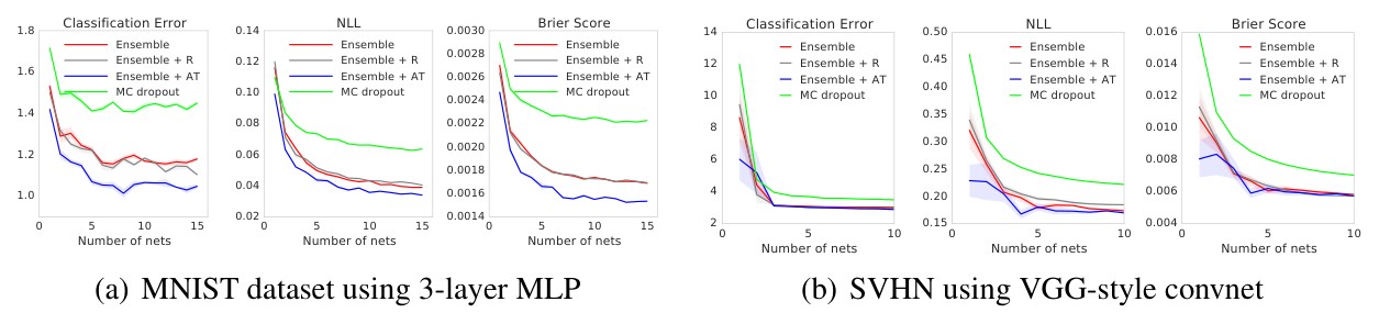 \n\nFigure 2: Evaluating predictive uncertainty as a function of ensemble size (number of networks in the ensemble or the number of MC-dropout samples): Ensemble variants significantly outperform MC-dropout performance with the corresponding in terms of all 3 metrics. Adversarial training improves results for MNIST for all and SVHN when , but the effect drops as increases.
图 2:预测不确定性随集成规模 (集成中的网络个数,或 MC-dropout 的样本数)变化的评估:在全部 3 项指标上,各集成变体都显著优于对应 的 MC-dropout。对抗训练对 MNIST 在所有 上都有改进,对 SVHN 则在 时有改进,但随着 增大,这一效果减弱。
We also report results on the SVHN dataset using an VGG-style convolutional NN.(^8) The results are in Figure 2(b). Ensembles outperform MC dropout. Adversarial training helps slightly for , however the effect drops as the number of networks in the ensemble increases. If the classes are well-separated, adversarial training might not change the classification boundary significantly. It is not clear if this is the case here, further investigation is required.
我们还用一个 VGG 风格的卷积网络在 SVHN 数据集上报告了结果。(^8) 结果见图 2(b)。集成优于 MC dropout。对抗训练在 时略有帮助,但随着集成中网络个数增加,这一效果减弱。如果各类分得较开,对抗训练可能并不会显著改变分类边界。此处是否属于这种情况并不清楚,还需要进一步研究。
The architecture is similar to the one described in http://torch.ch/blog/2015/07/30/cifar.html.
该结构与 http://torch.ch/blog/2015/07/30/cifar.html 中所述的结构类似。
Finally, we evaluate on the ImageNet (ILSVRC-2012) dataset [51] using the inception network [56]. Due to computational constraints, we only evaluate the effect of ensembles on this dataset. The results on ImageNet (single-crop evaluation) are shown in Table 4. We observe that as increases, both the accuracy and the quality of predictive uncertainty improve significantly.
最后,我们用 inception 网络 [56] 在 ImageNet(ILSVRC-2012)数据集 [51] 上做评估。由于计算限制,我们在该数据集上只评估集成的效果。ImageNet(单裁剪评估)上的结果见表 4。我们观察到,随着 增大,准确率和预测不确定性的质量都显著提高。
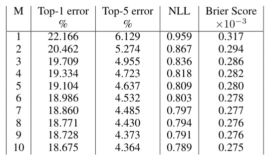 \n\nFigure 4: Results on ImageNet: Deep Ensembles lead to lower classification error as well as better predictive uncertainty as evidenced by lower NLL and Brier score.
图 4:ImageNet 上的结果:深度集成带来更低的分类误差,以及更好的预测不确定性,依据是更低的 NLL 和 Brier 分数。
Another advantage of using an ensemble is that it enables us to easily identify training examples where the individual networks disagree or agree the most. This disagreement(^9) provides another useful qualitative way to evaluate predictive uncertainty. Figures 10 and 11 in Appendix B.2 report qualitative evaluation of predictive uncertainty on the MNIST dataset.
使用集成的另一个好处是,我们可以很容易地找出各个网络分歧最大或最一致的训练样本。这种分歧(^9) 为评估预测不确定性提供了另一种有用的定性途径。附录 B.2 中的图 10 和图 11 报告了 MNIST 数据集上预测不确定性的定性评估。
More precisely, we define disagreement as where denotes the Kullback-Leibler divergence and is the prediction of the ensemble.
更精确地说,我们把分歧定义为 ,其中 表示 Kullback-Leibler 散度, 是集成的预测。
3.5 Uncertainty evaluation: test examples from known vs unknown classes
3.5 不确定性评估:来自已知类与未知类的测试样本
In the final experiment, we evaluate uncertainty on out-of-distribution examples from unseen classes. Overconfident predictions on unseen classes pose a challenge for reliable deployment of deep learning models in real world applications. We would like the predictions to exhibit higher uncertainty when the test data is very different from the training data. To test if the proposed method possesses this desirable property, we train a MLP on the standard MNIST train/test split using the same architecture as before. However, in addition to the regular test set with known classes, we also evaluate it on a test set containing unknown classes. We used the test split of the NotMNIST(^{10}) dataset.
在最后一项实验中,我们在来自未见类别的分布外样本上评估不确定性。在未见类别上给出过度自信的预测,会给深度学习模型在真实应用中的可靠部署带来挑战。我们希望当测试数据与训练数据差异很大时,预测能表现出更高的不确定度。为了检验所提方法是否具备这一可取性质,我们用与前面相同的结构,在标准的 MNIST 训练/测试划分上训练一个 MLP。不过,除了含已知类的常规测试集,我们还在一个含未知类的测试集上评估。我们使用的是 NotMNIST(^{10}) 数据集的测试划分。
The images in this dataset have the same size as MNIST, however the labels are alphabets instead of digits. We do not have access to the true conditional probabilities, but we expect the predictions to be closer to uniform on unseen classes compared to the known classes where the predictive probabilities should concentrate on the true targets. We evaluate the entropy of the predictive distribution and use this to evaluate the quality of the uncertainty estimates. The results are shown in Figure 3(a). For known classes (top row), both our method and MC-dropout have low entropy as expected. For unknown classes (bottom row), as increases, the entropy of deep ensembles increases much faster than MC-dropout indicating that our method is better suited for handling unseen test examples. In particular, MC-dropout seems to give high confidence predictions for some of the test examples, as evidenced by the mode around 0 even for unseen classes. Such overconfident wrong predictions can be problematic in practice when tested on a mixture of known and unknown classes, as we will see in Section 3.6. Comparing different variants of our method, the mode for adversarial training increases slightly faster than the mode for vanilla ensembles indicating that adversarial training is beneficial for quantifying uncertainty on unseen classes.
该数据集中的图像与 MNIST 尺寸相同,但标签是字母而不是数字。我们无法获得真实的条件概率,但我们预期,与已知类上预测概率应集中在真实目标附近相比,未见类上的预测应更接近均匀。我们评估预测分布的熵,并用它来衡量不确定性估计的质量。结果见图 3(a)。对已知类(上行),我们的方法和 MC-dropout 都如预期那样熵较低。对未知类(下行),随着 增大,深度集成的熵比 MC-dropout 上升得快得多,表明该方法更适合处理未见的测试样本。特别是,MC-dropout 似乎对部分测试样本给出了高置信度预测,证据是即便在未见类上,熵在 0 附近仍有一个众数。在由已知类和未知类混合而成的测试中,这类过度自信的错误预测在实践中可能造成问题,我们将在第 3.6 节看到这一点。比较该方法的不同变体,对抗训练对应的众数比普通集成上升得稍快一些,表明对抗训练有助于量化未见类上的不确定性。
We qualitatively evaluate results in Figures 12(a) and 12(b) in Appendix B.2. Figure 12(a) shows that the ensemble agreement is highest for letter ‘I’ which resembles 1 in the MNIST training dataset, and that the ensemble disagreement is higher for examples visually different from the MNIST training dataset.
我们在附录 B.2 的图 12(a) 和 12(b) 中对结果做了定性评估。图 12(a) 表明,集成一致性在字母 “I” 上最高,因为它与 MNIST 训练集中的 1 很像;而对视觉上与 MNIST 训练数据不同的样本,集成分歧更高。
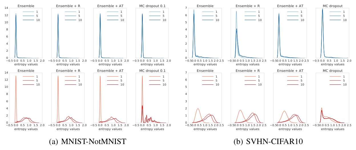 \n\nFigure 3: : Histogram of the predictive entropy on test examples from known classes (top row) and unknown classes (bottom row), as we vary ensemble size .
图 3:在来自已知类(上行)与未知类(下行)的测试样本上,预测熵的直方图,随集成规模 变化。
We ran a similar experiment, training on SVHN and testing on CIFAR-10 [31] test set; both datasets contain images, however SVHN contains images of digits whereas CIFAR-10 contains images of object categories. The results are shown in Figure 3(b). As in the MNIST-NotMNIST experiment, we observe that MC-dropout produces over-confident predictions on unseen examples, whereas our method produces higher uncertainty on unseen classes.
我们还做了类似实验:在 SVHN 上训练,在 CIFAR-10 [31] 测试集上测试;两个数据集都包含 的图像,但 SVHN 是数字图像,CIFAR-10 则是物体类别的图像。结果见图 3(b)。与 MNIST-NotMNIST 实验一样,我们观察到 MC-dropout 会在未见样本上给出过度自信的预测,而我们的方法在未见类上给出更高的不确定度。
Finally, we test on ImageNet by splitting the training set by categories. We split the dataset into images of dogs (known classes) and non-dogs (unknown classes), following Vinyals et al. [58] who proposed this setup for a different task. Figure 5 shows the histogram of the predictive entropy as well as the maximum predicted probability (i.e. confidence in the predicted class). We observe that the predictive uncertainty improves on unseen classes, as the ensemble size increases.
最后,我们按类别划分训练集,在 ImageNet 上做测试。我们把数据分成狗的图像(已知类)和非狗的图像(未知类),这一设定沿用了 Vinyals 等人 [58] 为另一任务提出的做法。图 5 给出了预测熵以及最大预测概率(即对预测类别的置信度)的直方图。我们观察到,随着集成规模增大,未见类上的预测不确定性有所改进。
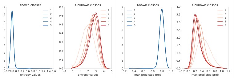 \n\nFigure 5: ImageNet trained only on dogs: Histogram of the predictive entropy (left) and maximum predicted probability (right) on test examples from known classes (dogs) and unknown classes (non-dogs), as we vary the ensemble size.
图 5:仅在狗的类别上训练的 ImageNet:在来自已知类(狗)与未知类(非狗)的测试样本上,预测熵(左)和最大预测概率(右)的直方图,随集成规模变化。
3.6 Accuracy as a function of confidence
3.6 准确率随置信度的变化
In practical applications, it is highly desirable for a system to avoid overconfident, incorrect predictions and fail gracefully. To evaluate the usefulness of predictive uncertainty for decision making, we consider a task where the model is evaluated only on cases where the model’s confidence is above an user-specified threshold. If the confidence estimates are well-calibrated, one can trust the model’s predictions when the reported confidence is high and resort to a different solution (e.g. use human in a loop, or use prediction from a simpler model) when the model is not confident.
在实际应用中,系统最好能避免过度自信的错误预测,并做到平稳失效。为了评估预测不确定性对决策的用处,我们考虑这样一项任务:只在模型置信度高于用户指定阈值的情形下评估模型。如果置信度估计校准良好,就可以在报告的置信度高时采信模型的预测,而在模型不自信时改用其他方案(例如引入人工,或改用更简单模型的预测)。
We re-use the results from the experiment in the previous section where we trained a network on MNIST and test it on a mix of test examples from MNIST (known classes) and NotMNIST (unknown classes). The network will produce incorrect predictions on out-of-distribution examples, however we would like these predictions to have low confidence. Given the prediction , we define the predicted label as , and the confidence as . We filter out test examples, corresponding to a particular confidence threshold and plot the accuracy for this threshold. The confidence vs accuracy results are shown in Figure 6. If we look at cases only where the confidence is , we expect higher accuracy than cases where confidence , hence the curve should be monotonically increasing. If the application demands an accuracy , we can trust the model only in cases where the confidence is greater than the corresponding threshold. Hence, we can compare accuracy of the models for a desired confidence threshold of the application. MC-dropout can produce overconfident wrong predictions as evidenced by low accuracy even for high values of , whereas deep ensembles are significantly more robust.
我们复用上一节实验的结果:网络在 MNIST 上训练,并在 MNIST(已知类)与 NotMNIST(未知类)混合而成的测试样本上测试。网络会在分布外样本上给出错误预测,但我们希望这些预测的置信度较低。给定预测 ,我们把预测标签定义为 ,把置信度定义为 。我们按某一置信度阈值 筛出测试样本,并画出该阈值下的准确率。置信度与准确率的结果见图 6。如果只看置信度 的情形,我们预期准确率会高于置信度 的情形,因此这条曲线应当单调上升。若应用要求准确率达到 ,我们就只在置信度高于相应阈值时采信模型。由此,我们可以按应用所希望的置信度阈值来比较各模型的准确率。MC-dropout 可能给出过度自信的错误预测,证据是即便在 很高时准确率仍然偏低;而深度集成要稳健得多。
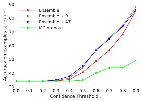 \n\nFigure 6: Accuracy vs Confidence curves: Networks trained on MNIST and tested on both MNIST test containing known classes and the NotMNIST dataset containing unseen classes. MC-dropout can produce overconfident wrong predictions, whereas deep ensembles are significantly more robust.
图 6:准确率–置信度曲线:网络在 MNIST 上训练,并同时在含已知类的 MNIST 测试集和含未见类的 NotMNIST 数据集上测试。MC-dropout 可能给出过度自信的错误预测,而深度集成要稳健得多。
4 Discussion
4 讨论
We have proposed a simple and scalable non-Bayesian solution that provides a very strong baseline on evaluation metrics for predictive uncertainty quantification. Intuitively, our method captures two sources of uncertainty. Training a probabilistic NN using proper scoring rules as training objectives captures ambiguity in targets for a given . In addition, our method uses a combination of ensembles (which captures “model uncertainty” by averaging predictions over multiple models consistent with the training data), and adversarial training (which encourages local smoothness), for robustness to model misspecification and out-of-distribution examples. Ensembles, even for , significantly improve uncertainty quality in all the cases. Adversarial training helps on some datasets for some metrics and is not strictly necessary in all cases. Our method requires very little hyperparameter tuning and is well suited for large scale distributed computation and can be readily implemented for a wide variety of architectures such as MLPs, CNNs, etc including those which do not use dropout e.g. residual networks [22]. It is perhaps surprising to the Bayesian deep learning community that a non-Bayesian (yet probabilistic) approach can perform as well as Bayesian NNs. We hope that our work will encourage the community to consider non-Bayesian approaches (such as ensembles) and other interesting evaluation metrics for predictive uncertainty. Concurrent with our work, Hendrycks and Gimpel [23] and Guo et al. [20] have also independently shown that non-Bayesian solutions can produce good predictive uncertainty estimates on some tasks. Abbasi and Gagné [1], Tramèr et al. [57] have also explored ensemble-based solutions to tackle adversarial examples, a particularly hard case of out-of-distribution examples.
我们提出了一种简单、可扩展的非贝叶斯方案,在预测不确定性量化的评价指标上提供了一个很强的基线。直观上,该方法捕捉两类不确定性。用适当评分规则作为训练目标来训练概率神经网络 ,捕捉的是给定 时目标 中的含混。此外,该方法还把集成(通过在与训练数据相符的多个模型上平均预测,来捕捉“模型不确定性”)和对抗训练(鼓励局部平滑)结合起来,以增强对模型设定偏差和分布外样本的稳健性。即便 ,集成在所有情形下都显著提高了不确定性的质量。对抗训练在部分数据集、部分指标上有帮助,但并非在所有情形下都必不可少。该方法几乎不必调超参数,很适合大规模分布式计算,也易于在多种多样的结构上实现,例如 MLP、CNN 等,包括那些并不使用 dropout 的结构,如残差网络 [22]。对贝叶斯深度学习社区而言,一种非贝叶斯(但仍是概率的)方法能与贝叶斯神经网络表现相当,也许会令人意外。我们希望这项工作能促使社区更多地考虑非贝叶斯方法(例如集成),以及其他有意思的预测不确定性评价指标。与我们的工作同时,Hendrycks 和 Gimpel [23] 以及 Guo 等人 [20] 也独立表明,非贝叶斯方案能在部分任务上给出良好的预测不确定性估计。Abbasi 和 Gagné [1]、Tramèr 等人 [57] 也探索了基于集成的方案,用以应对对抗样本这一类特别困难的分布外情形。
There are several avenues for future work. We focused on training independent networks as training can be trivially parallelized. Explicitly de-correlating networks’ predictions, e.g. as in [37], might promote ensemble diversity and improve performance even further. Optimizing the ensemble weights, as in stacking [60] or adaptive mixture of experts [28], can further improve the performance. The ensemble has times more parameters than a single network; for memory-constrained applications, the ensemble can be distilled into a simpler model [10, 26]. It would be also interesting to investigate so-called implicit ensembles the where ensemble members share parameters, e.g. using multiple heads [36, 48], snapshot ensembles [27] or swapout [52].
未来工作还有若干方向。我们着重训练相互独立的网络,因为这样训练可以很容易地并行化。显式地降低各网络预测之间的相关性,例如像 [37] 那样,也许能促进集成多样性,并进一步提高表现。像堆叠 [60] 或自适应专家混合 [28] 那样优化集成权重,也能进一步改进表现。集成的参数量是单个网络的 倍;对内存受限的应用,可以把集成蒸馏成更简单的模型 [10, 26]。所谓隐式集成,即成员共享参数的集成,例如使用多个头 [36, 48]、snapshot ensembles [27] 或 swapout [52],也值得研究。
Acknowledgments
致谢
We would like to thank Samuel Ritter and Oriol Vinyals for help with ImageNet experiments, and Daan Wierstra, David Silver, David Barrett, Ian Osband, Martin Szummer, Peter Dayan, Shakir Mohamed, Theophane Weber, Ulrich Paquet and the anonymous reviewers for helpful feedback.
感谢 Samuel Ritter 和 Oriol Vinyals 在 ImageNet 实验上的帮助,并感谢 Daan Wierstra、David Silver、David Barrett、Ian Osband、Martin Szummer、Peter Dayan、Shakir Mohamed、Theophane Weber、Ulrich Paquet 以及匿名审稿人的有益反馈。
References
参考文献
[1] M. Abbasi and C. Gagné. Robustness to adversarial examples through an ensemble of specialists. arXiv preprint arXiv:1702.06856, 2017.
[2] B. Alipanahi, A. Delong, M. T. Weirauch, and B. J. Frey. Predicting the sequence specificities of DNA-and RNA-binding proteins by deep learning. Nature biotechnology, 33(8):831–838, 2015.
[3] D. Amodei, C. Olah, J. Steinhardt, P. Christiano, J. Schulman, and D. Mané. Concrete problems in AI safety. arXiv preprint arXiv:1606.06565, 2016.
[4] J. M. Bernardo and A. F. Smith. Bayesian Theory, volume 405. John Wiley & Sons, 2009.
[5] C. M. Bishop. Mixture density networks. 1994.
[6] C. Blundell, J. Cornebise, K. Kavukcuoglu, and D. Wierstra. Weight uncertainty in neural networks. In ICML, 2015.
[7] L. Breiman. Bagging predictors. Machine learning, 24(2):123–140, 1996.
[8] L. Breiman. Random forests. Machine learning, 45(1):5–32, 2001.
[9] G. W. Brier. Verification of forecasts expressed in terms of probability. Monthly weather review, 1950.
[10] C. Bucila, R. Caruana, and A. Niculescu-Mizil. Model compression. In KDD. ACM, 2006.
[11] B. Clarke. Comparing Bayes model averaging and stacking when model approximation error cannot be ignored. J. Mach. Learn. Res. (JMLR), 4:683–712, 2003.
[12] A. P. Dawid. The well-calibrated Bayesian. Journal of the American Statistical Association, 1982.
[13] M. H. DeGroot and S. E. Fienberg. The comparison and evaluation of forecasters. The statistician, 1983.
[14] T. G. Dietterich. Ensemble methods in machine learning. In Multiple classifier systems. 2000.
[15] Y. Gal and Z. Ghahramani. Dropout as a Bayesian approximation: Representing model uncertainty in deep learning. In ICML, 2016.
[16] P. Geurts, D. Ernst, and L. Wehenkel. Extremely randomized trees. Machine learning, 63(1):3–42, 2006.
[17] T. Gneiting and A. E. Raftery. Strictly proper scoring rules, prediction, and estimation. Journal of the American Statistical Association, 102(477):359–378, 2007.
[18] I. J. Goodfellow, J. Shlens, and C. Szegedy. Explaining and harnessing adversarial examples. In ICLR, 2015.
[19] A. Graves. Practical variational inference for neural networks. In NIPS, 2011.
[20] C. Guo, G. Pleiss, Y. Sun, and K. Q. Weinberger. On calibration of modern neural networks. arXiv preprint arXiv:1706.04599, 2017.
[21] L. Hasenclever, S. Webb, T. Lienart, S. Vollmer, B. Lakshminarayanan, C. Blundell, and Y. W. Teh. Distributed Bayesian learning with stochastic natural-gradient expectation propagation and the posterior server. arXiv preprint arXiv:1512.09327, 2015.
[22] K. He, X. Zhang, S. Ren, and J. Sun. Deep residual learning for image recognition. In Proceedings of the IEEE Conference on Computer Vision and Pattern Recognition, pages 770–778, 2016.
[23] D. Hendrycks and K. Gimpel. A baseline for detecting misclassified and out-of-distribution examples in neural networks. arXiv preprint arXiv:1610.02136, 2016.
[24] J. M. Hernández-Lobato and R. P. Adams. Probabilistic backpropagation for scalable learning of Bayesian neural networks. In ICML, 2015.
[25] G. Hinton, L. Deng, D. Yu, G. E. Dahl, A.-r. Mohamed, N. Jaitly, A. Senior, V. Vanhoucke, P. Nguyen, T. N. Sainath, et al. Deep neural networks for acoustic modeling in speech recog- nition: The shared views of four research groups. Signal Processing Magazine, IEEE, 29(6): 82–97, 2012.
[26] G. Hinton, O. Vinyals, and J. Dean. Distilling the knowledge in a neural network. arXiv preprint arXiv:1503.02531, 2015.
[27] G. Huang, Y. Li, G. Pleiss, Z. Liu, J. E. Hopcroft, and K. Q. Weinberger. Snapshot ensembles: Train 1, get M for free. ICLR submission, 2017.
[28] R. A. Jacobs, M. I. Jordan, S. J. Nowlan, and G. E. Hinton. Adaptive mixtures of local experts. Neural computation, 3(1):79–87, 1991.
[29] D. P. Kingma, T. Salimans, and M. Welling. Variational dropout and the local reparameterization trick. In NIPS, 2015.
[30] A. Korattikara, V. Rathod, K. Murphy, and M. Welling. Bayesian dark knowledge. In NIPS, 2015.
[31] A. Krizhevsky. Learning multiple layers of features from tiny images. 2009.
[32] A. Krizhevsky, I. Sutskever, and G. E. Hinton. Imagenet classification with deep convolutional neural networks. In NIPS, 2012.
[33] A. Kurakin, I. Goodfellow, and S. Bengio. Adversarial machine learning at scale. arXiv preprint arXiv:1611.01236, 2016.
[34] B. Lakshminarayanan. Decision trees and forests: a probabilistic perspective. PhD thesis, UCL (University College London), 2016.
[35] Y. LeCun, Y. Bengio, and G. Hinton. Deep learning. Nature, 521(7553):436–444, 2015.
[36] S. Lee, S. Purushwalkam, M. Cogswell, D. Crandall, and D. Batra. Why M heads are better than one: Training a diverse ensemble of deep networks. arXiv preprint arXiv:1511.06314, 2015.
[37] S. Lee, S. P. S. Prakash, M. Cogswell, V. Ranjan, D. Crandall, and D. Batra. Stochastic multiple choice learning for training diverse deep ensembles. In NIPS, 2016.
[38] Y. Li, J. M. Hernández-Lobato, and R. E. Turner. Stochastic expectation propagation. In NIPS, 2015.
[39] C. Louizos and M. Welling. Structured and efficient variational deep learning with matrix Gaussian posteriors. arXiv preprint arXiv:1603.04733, 2016.
[40] D. J. MacKay. Bayesian methods for adaptive models. PhD thesis, California Institute of Technology, 1992.
[41] S.-i. Maeda. A Bayesian encourages dropout. arXiv preprint arXiv:1412.7003, 2014.
[42] T. Mikolov, K. Chen, G. Corrado, and J. Dean. Efficient estimation of word representations in vector space. arXiv preprint arXiv:1301.3781, 2013.
[43] T. P. Minka. Bayesian model averaging is not model combination. 2000.
[44] T. Miyato, S.-i. Maeda, M. Koyama, K. Nakae, and S. Ishii. Distributional smoothing by virtual adversarial examples. In ICLR, 2016.
[45] V. Nair and G. E. Hinton. Rectified linear units improve restricted Boltzmann machines. In ICML, 2010.
[46] R. M. Neal. Bayesian Learning for Neural Networks. Springer-Verlag New York, Inc., 1996.
[47] D. A. Nix and A. S. Weigend. Estimating the mean and variance of the target probability distribution. In IEEE International Conference on Neural Networks, 1994.
[48] I. Osband, C. Blundell, A. Pritzel, and B. Van Roy. Deep exploration via bootstrapped DQN. In NIPS, 2016.
[49] J. Quinonero-Candela, C. E. Rasmussen, F. Sinz, O. Bousquet, and B. Schölkopf. Evaluating predictive uncertainty challenge. In Machine Learning Challenges. Springer, 2006.
[50] C. E. Rasmussen and J. Quinonero-Candela. Healing the relevance vector machine through augmentation. In ICML, 2005.
[51] O. Russakovsky, J. Deng, H. Su, J. Krause, S. Satheesh, S. Ma, Z. Huang, A. Karpathy, A. Khosla, M. Bernstein, A. C. Berg, and L. Fei-Fei. ImageNet Large Scale Visual Recognition Challenge. International Journal of Computer Vision (IJCV), 115(3):211–252, 2015.
[52] S. Singh, D. Hoiem, and D. Forsyth. Swapout: Learning an ensemble of deep architectures. In NIPS, 2016.
[53] J. T. Springenberg, A. Klein, S. Falkner, and F. Hutter. Bayesian optimization with robust Bayesian neural networks. In Advances in Neural Information Processing Systems, pages 4134–4142, 2016.
[54] N. Srivastava, G. Hinton, A. Krizhevsky, I. Sutskever, and R. Salakhutdinov. Dropout: A simple way to prevent neural networks from overfitting. JMLR, 2014.
[55] C. Szegedy, W. Zaremba, I. Sutskever, J. Bruna, D. Erhan, I. Goodfellow, and R. Fergus. Intriguing properties of neural networks. In ICLR, 2014.
[56] C. Szegedy, V. Vanhoucke, S. Ioffe, J. Shlens, and Z. Wojna. Rethinking the inception architecture for computer vision. In Proceedings of the IEEE Conference on Computer Vision and Pattern Recognition, pages 2818–2826, 2016.
[57] F. Tramèr, A. Kurakin, N. Papernot, D. Boneh, and P. McDaniel. Ensemble adversarial training: Attacks and defenses. arXiv preprint arXiv:1705.07204, 2017.
[58] O. Vinyals, C. Blundell, T. Lillicrap, D. Wierstra, et al. Matching networks for one shot learning. In NIPS, 2016.
[59] M. Welling and Y. W. Teh. Bayesian learning via stochastic gradient Langevin dynamics. In ICML, 2011.
[60] D. H. Wolpert. Stacked generalization. Neural networks, 5(2):241–259, 1992.
[61] J. Zhou and O. G. Troyanskaya. Predicting effects of noncoding variants with deep learning-based sequence model. Nature methods, 12(10):931–934, 2015.