DeBERTa: Decoding-enhanced BERT with Disentangled Attention
DeBERTa: Decoding-enhanced BERT with Disentangled Attention
DeBERTa:解码增强的 BERT 与解耦注意力
Pengcheng He Affiliation: Microsoft Dynamics 365 AI Email: penhe@microsoft.com Xiaodong Liu Affiliation: Microsoft Research Email: xiaodl@microsoft.com Jianfeng Gao Affiliation: Microsoft Research Email: jfgao@microsoft.com Weizhu Chen Affiliation: Microsoft Dynamics 365 AI Email: wzchen@microsoft.com
Abstract
摘要
Recent progress in pre-trained neural language models has significantly improved the performance of many natural language processing (NLP) tasks. In this paper we propose a new model architecture DeBERTa (Decoding-enhanced BERT with disentangled attention) that improves the BERT and RoBERTa models using two novel techniques. The first is the disentangled attention mechanism, where each word is represented using two vectors that encode its content and position, respectively, and the attention weights among words are computed using disentangled matrices on their contents and relative positions, respectively. Second, an enhanced mask decoder is used to incorporate absolute positions in the decoding layer to predict the masked tokens in model pre-training. In addition, a new virtual adversarial training method is used for fine-tuning to improve models’ generalization. We show that these techniques significantly improve the efficiency of model pre-training and the performance of both natural language understand (NLU) and natural langauge generation (NLG) downstream tasks. Compared to RoBERTa-Large, a DeBERTa model trained on half of the training data performs consistently better on a wide range of NLP tasks, achieving improvements on MNLI by +0.9% (90.2% vs. 91.1%), on SQuAD v2.0 by +2.3% (88.4% vs. 90.7%) and RACE by +3.6% (83.2% vs. 86.8%). Notably, we scale up DeBERTa by training a larger version that consists of 48 Transform layers with 1.5 billion parameters. The significant performance boost makes the single DeBERTa model surpass the human performance on the SuperGLUE benchmark (Wang et al., 2019a) for the first time in terms of macro-average score (89.9 versus 89.8), and the ensemble DeBERTa model sits atop the SuperGLUE leaderboard as of January 6, 2021, outperforming the human baseline by a decent margin (90.3 versus 89.8). The pre-trained DeBERTa models and the source code were released at: https://github.com/microsoft/DeBERTa[^1].
预训练神经语言模型的进展显著提升了许多自然语言处理(NLP)任务的表现。本文提出新架构 DeBERTa(Decoding-enhanced BERT with disentangled attention),用两项新技术改进 BERT 与 RoBERTa。其一是解耦注意力机制:每个词分别用内容向量与位置向量表示,词间注意力权重由内容与相对位置上的解耦矩阵分别计算。其二是增强掩码解码器:在解码层引入绝对位置,以在预训练中预测被掩码词元。此外,微调时使用一种新的虚拟对抗训练以提升泛化。我们表明这些技术显著提高了预训练效率,以及自然语言理解(NLU)与自然语言生成(NLG)下游任务的表现。相对 RoBERTa-Large,仅用一半训练数据训练的 DeBERTa 在广泛 NLP 任务上持续更优:MNLI +0.9%(90.2% vs. 91.1%),SQuAD v2.0 +2.3%(88.4% vs. 90.7%),RACE +3.6%(83.2% vs. 86.8%)。我们还将 DeBERTa 扩展为含 48 个 Transformer 层、15 亿参数的更大版本。性能提升使单模型 DeBERTa 首次在 SuperGLUE 基准(Wang et al., 2019a)宏平均上超过人类表现(89.9 vs. 89.8);截至 2021 年 1 月 6 日,集成 DeBERTa 位居 SuperGLUE 榜首,相对人类基线优势明显(90.3 vs. 89.8)。预训练模型与源码发布于:https://github.com/microsoft/DeBERTa[^1]。
1 Introduction
1 引言
The Transformer has become the most effective neural network architecture for neural language modeling. Unlike recurrent neural networks (RNNs) that process text in sequence, Transformers apply self-attention to compute in parallel every word from the input text an attention weight that gauges the influence each word has on another, thus allowing for much more parallelization than RNNs for large-scale model training (Vaswani et al., 2017). Since 2018, we have seen the rise of a set of large-scale Transformer-based Pre-trained Language Models (PLMs), such as GPT (Radford et al., 2019; Brown et al., 2020), BERT (Devlin et al., 2019), RoBERTa (Liu et al., 2019c), XLNet (Yang et al., 2019), UniLM (Dong et al., 2019), ELECTRA (Clark et al., 2020), T5 (Raffel et al., 2020), ALUM (Liu et al., 2020), StructBERT (Wang et al., 2019c) and ERINE (Sun et al., 2019) . These PLMs have been fine-tuned using task-specific labels and created new state of the art in many downstream natural language processing (NLP) tasks (Liu et al., 2019b; Minaee et al., 2020; Jiang et al., 2020; He et al., 2019a; He et al., 2019b; Shen et al., 2020).
Transformer 已成为神经语言建模最有效的神经网络架构。与按序处理文本的循环神经网络(RNN)不同,Transformer 用自注意力并行计算输入文本中每个词对其他词的影响权重,因而在大规模模型训练上比 RNN 可并行性高得多(Vaswani et al., 2017)。自 2018 年起,出现一批大规模基于 Transformer 的预训练语言模型(PLM),如 GPT(Radford et al., 2019;Brown et al., 2020)、BERT(Devlin et al., 2019)、RoBERTa(Liu et al., 2019c)、XLNet(Yang et al., 2019)、UniLM(Dong et al., 2019)、ELECTRA(Clark et al., 2020)、T5(Raffel et al., 2020)、ALUM(Liu et al., 2020)、StructBERT(Wang et al., 2019c)与 ERINE(Sun et al., 2019)。这些 PLM 经任务标签微调后,在许多下游 NLP 任务上创造了新的最优结果(Liu et al., 2019b;Minaee et al., 2020;Jiang et al., 2020;He et al., 2019a;He et al., 2019b;Shen et al., 2020)。
In this paper, we propose a new Transformer-based neural language model DeBERTa (Decoding-enhanced BERT with disentangled attention), which improves previous state-of-the-art PLMs using two novel techniques: a disentangled attention mechanism, and an enhanced mask decoder.
本文提出基于 Transformer 的神经语言模型 DeBERTa(Decoding-enhanced BERT with disentangled attention),用两项新技术改进先前最优 PLM:解耦注意力机制,以及增强掩码解码器。
Disentangled attention.
Unlike BERT where each word in the input layer is represented using a vector which is the sum of its word (content) embedding and position embedding, each word in DeBERTa is represented using two vectors that encode its content and position, respectively, and the attention weights among words are computed using disentangled matrices based on their contents and relative positions, respectively. This is motivated by the observation that the attention weight of a word pair depends on not only their contents but their relative positions. For example, the dependency between the words “deep” and “learning” is much stronger when they occur next to each other than when they occur in different sentences.
解耦注意力。
与 BERT 在输入层用词(内容)嵌入与位置嵌入之和表示每个词不同,DeBERTa 用两个向量分别编码内容与位置,词间注意力权重由基于内容与相对位置的解耦矩阵分别计算。动机是:词对的注意力权重不仅依赖内容,也依赖相对位置。例如,“deep”与“learning”相邻出现时的依存远强于它们出现在不同句子中时。
Enhanced mask decoder.
Like BERT, DeBERTa is pre-trained using masked language modeling (MLM). MLM is a fill-in-the-blank task, where a model is taught to use the words surrounding a mask token to predict what the masked word should be. DeBERTa uses the content and position information of the context words for MLM. The disentangled attention mechanism already considers the contents and relative positions of the context words, but not the absolute positions of these words, which in many cases are crucial for the prediction. Consider the sentence “a new store opened beside the new mall” with the italicized words “store” and “mall” masked for prediction. Although the local contexts of the two words are similar, they play different syntactic roles in the sentence. (Here, the subject of the sentence is “store” not “mall,” for example.) These syntactical nuances depend, to a large degree, upon the words’ absolute positions in the sentence, and so it is important to account for a word’s absolute position in the language modeling process. DeBERTa incorporates absolute word position embeddings right before the softmax layer where the model decodes the masked words based on the aggregated contextual embeddings of word contents and positions.
增强掩码解码器。
与 BERT 一样,DeBERTa 用掩码语言建模(MLM)预训练。MLM 是填空任务:模型学习用掩码词元周围的词预测被掩词。DeBERTa 对 MLM 使用上下文词的内容与位置信息。解耦注意力已考虑上下文词的内容与相对位置,但未考虑其绝对位置,而这在许多情况下对预测至关重要。考虑句子 “a new store opened beside the new mall”,其中斜体 “store” 与 “mall” 被掩以待预测。两词局部上下文相似,但句法角色不同(主语是 “store” 而非 “mall”)。这些句法细微差别在很大程度上依赖词在句中的绝对位置,因此语言建模过程需要计入绝对位置。DeBERTa 在 softmax 层之前引入绝对词位置嵌入,使模型基于词内容与位置的聚合上下文嵌入解码被掩词。
In addition, we propose a new virtual adversarial training method for fine-tuning PLMs to downstream NLP tasks. The method is effective in improving models’ generalization.
此外,我们提出一种新的虚拟对抗训练方法,用于将 PLM 微调到下游 NLP 任务。该方法能有效提升模型泛化。
We show through a comprehensive empirical study that these techniques substantially improve the efficiency of pre-training and the performance of downstream tasks. In the NLU tasks, compared to RoBERTa-Large, a DeBERTa model trained on half the training data performs consistently better on a wide range of NLP tasks, achieving improvements on MNLI by +0.9% (90.2% vs. 91.1%), on SQuAD v2.0 by +2.3%(88.4% vs. 90.7%), and RACE by +3.6% (83.2% vs. 86.8%). In the NLG tasks, DeBERTa reduces the perplexity from 21.6 to 19.5 on the Wikitext-103 dataset. We further scale up DeBERTa by pre-training a larger model that consists of 48 Transformer layers with 1.5 billion parameters. The single 1.5B-parameter DeBERTa model substantially outperforms T5 with 11 billion parameters on the SuperGLUE benchmark (Wang et al., 2019a) by 0.6%(89.3% vs. 89.9%), and surpasses the human baseline (89.9 vs. 89.8) for the first time. The ensemble DeBERTa model sits atop the SuperGLUE leaderboard as of January 6, 2021, outperforming the human baseline by a decent margin (90.3 versus 89.8).
全面实证表明,这些技术显著提升预训练效率与下游表现。在 NLU 任务上,相对 RoBERTa-Large,半数据训练的 DeBERTa 在广泛任务上持续更优:MNLI +0.9%(90.2% vs. 91.1%),SQuAD v2.0 +2.3%(88.4% vs. 90.7%),RACE +3.6%(83.2% vs. 86.8%)。在 NLG 任务上,DeBERTa 把 Wikitext-103 的困惑度从 21.6 降到 19.5。我们进一步预训练含 48 个 Transformer 层、15 亿参数的更大模型。单模型 15 亿参数 DeBERTa 在 SuperGLUE(Wang et al., 2019a)上相对 110 亿参数的 T5 高出 0.6%(89.3% vs. 89.9%),并首次超过人类基线(89.9 vs. 89.8)。截至 2021 年 1 月 6 日,集成 DeBERTa 位居 SuperGLUE 榜首,相对人类基线优势明显(90.3 vs. 89.8)。
2 Background
2 背景
2.1 Transformer
A Transformer-based language model is composed of stacked Transformer blocks (Vaswani et al., 2017). Each block contains a multi-head self-attention layer followed by a fully connected positional feed-forward network. The standard self-attention mechanism lacks a natural way to encode word position information. Thus, existing approaches add a positional bias to each input word embedding so that each input word is represented by a vector whose value depends on its content and position. The positional bias can be implemented using absolute position embedding (Vaswani et al., 2017; Radford et al., 2019; Devlin et al., 2019) or relative position embedding (Huang et al., 2018; Yang et al., 2019). It has been shown that relative position representations are more effective for natural language understanding and generation tasks (Dai et al., 2019; Shaw et al., 2018). The proposed disentangled attention mechanism differs from all existing approaches in that we represent each input word using two separate vectors that encode a word’s content and position, respectively, and attention weights among words are computed using disentangled matrices on their contents and relative positions, respectively.
基于 Transformer 的语言模型由堆叠的 Transformer 块组成(Vaswani et al., 2017)。每块含多头自注意力层,后接全连接的位置前馈网络。标准自注意力缺乏自然编码词位置信息的方式。因此现有方法给每个输入词嵌入加位置偏置,使每个输入词由依赖其内容与位置的向量表示。位置偏置可用绝对位置嵌入(Vaswani et al., 2017;Radford et al., 2019;Devlin et al., 2019)或相对位置嵌入(Huang et al., 2018;Yang et al., 2019)实现。已有工作表明相对位置表示对自然语言理解与生成任务更有效(Dai et al., 2019;Shaw et al., 2018)。所提解耦注意力与既有方法都不同:我们用两个分离向量分别编码词的内容与位置,词间注意力权重由内容与相对位置上的解耦矩阵分别计算。
2.2 Masked Language Model
2.2 掩码语言模型
Large-scale Transformer-based PLMs are typically pre-trained on large amounts of text to learn contextual word representations using a self-supervision objective, known as Masked Language Model (MLM) (Devlin et al., 2019). Specifically, given a sequence , we corrupt it into by masking 15% of its tokens at random and then train a language model parameterized by to reconstruct by predicting the masked tokens conditioned on :
大规模基于 Transformer 的 PLM 通常在大量文本上用自监督目标——掩码语言模型(MLM)(Devlin et al., 2019)——预训练以学习上下文词表征。具体地,给定序列 ,我们随机掩码 15% 词元得到损坏序列 ,再训练参数为 的语言模型,在条件 下预测被掩词元 以重建 :
where is the index set of the masked tokens in the sequence. The authors of BERT propose to keep 10% of the masked tokens unchanged, another 10% replaced with randomly picked tokens and the rest replaced with the [MASK] token.
其中 是序列中被掩词元的下标集合。BERT 作者提议:10% 被掩词元保持不变,另 10% 换为随机词元,其余换为 [MASK] 词元。
3 The DeBERTa Architecture
3 DeBERTa 架构
3.1 Disentangled Attention: A Two-Vector Approach to Content and Position Embedding
3.1 解耦注意力:内容与位置嵌入的双向量方法
For a token at position in a sequence, we represent it using two vectors, and , which represent its content and relative position with the token at position , respectively. The calculation of the cross attention score between tokens and can be decomposed into four components as
对序列中位置 的词元,我们用两个向量 与 分别表示其内容,以及相对位置 词元的相对位置。词元 与 的交叉注意力分数可分解为四项:
$$\begin{split}A_{i,j}&={\bm{H_{i}},\bm{P_{i|j}}}\times{\bm{H_{j}},\bm{P_{j|i}}}^{\intercal}\
&=\bm{H_{i}}\bm{H_{j}}^{\intercal}+\bm{H_{i}}\bm{P_{j|i}}^{\intercal}+\bm{P_{i|j}}\bm{H_{j}}^{\intercal}+\bm{P_{i|j}}\bm{P_{j|i}}^{\intercal}\end{split} \tag{2}$$
That is, the attention weight of a word pair can be computed as a sum of four attention scores using disentangled matrices on their contents and positions as content-to-content, content-to-position, position-to-content, and position-to-position [^2].
也就是说,词对的注意力权重可写成内容与位置上四项解耦注意力分数之和:内容到内容、内容到位置、位置到内容,以及 位置到位置 [^2]。
Existing approaches to relative position encoding use a separate embedding matrix to compute the relative position bias in computing attention weights (Shaw et al., 2018; Huang et al., 2018). This is equivalent to computing the attention weights using only the content-to-content and content-to-position terms in equation 2. We argue that the position-to-content term is also important since the attention weight of a word pair depends not only on their contents but on their relative positions, which can only be fully modeled using both the content-to-position and position-to-content terms. Since we use relative position embedding, the position-to-position term does not provide much additional information and is removed from equation 2 in our implementation.
既有相对位置编码方法用单独嵌入矩阵在计算注意力权重时加入相对位置偏置(Shaw et al., 2018;Huang et al., 2018)。这等价于公式 2 中只用内容到内容与内容到位置两项。我们认为位置到内容项同样重要,因为词对注意力不仅依赖内容也依赖相对位置,而后者需同时用内容到位置与位置到内容才能充分建模。由于我们使用相对位置嵌入,位置到位置项提供的额外信息不多,实现中从公式 2 去掉该项。
Taking single-head attention as an example, the standard self-attention operation (Vaswani et al., 2017) can be formulated as:
以单头注意力为例,标准自注意力运算(Vaswani et al., 2017)可写为:
where represents the input hidden vectors, the output of self-attention, the projection matrices, the attention matrix, the length of the input sequence, and the dimension of hidden states.
其中 为输入隐向量, 为自注意力输出, 为投影矩阵, 为注意力矩阵, 为输入序列长度, 为隐状态维度。
Denote as the maximum relative distance, as the relative distance from token to token , which is defined as:
记 为最大相对距离, 为词元 到词元 的相对距离,定义为:
$$\delta(i,j)=\left{\begin{array}[]{rcl}0&\mbox{for}&i-j\leq-k\
2k-1&\mbox{for}&i-j\geq k\
i-j+k&\mbox{others}.\end{array}\right. \tag{3}$$
We can represent the disentangled self-attention with relative position bias as equation 4, where and are the projected content vectors generated using projection matrices respectively, represents the relative position embedding vectors shared across all layers (i.e., staying fixed during forward propagation), and and are projected relative position vectors generated using projection matrices , respectively.
带相对位置偏置的解耦自注意力可表示为公式 4,其中 与 分别由投影矩阵 生成的投影内容向量, 表示各层共享的相对位置嵌入向量(前向中保持固定), 与 分别由投影矩阵 生成的投影相对位置向量。
$$\begin{split}\bm{Q_{c}}=\bm{H}\bm{W_{q,c}},\bm{K_{c}}&=\bm{H}\bm{W_{k,c}},\bm{V_{c}}=\bm{H}\bm{W_{v,c}},\bm{Q_{r}}=\bm{P}\bm{W_{q,r}},\bm{K_{r}}=\bm{P}\bm{W_{k,r}}\
\tilde{A}{i,j}&=\underbrace{\bm{Q^{c}{i}}\bm{{K^{c}{j}}^{\intercal}}}{\text{(a) content-to-content}}+\underbrace{\bm{Q^{c}{i}}\bm{{K^{r}{\delta(i,j)}}^{\intercal}}}{\text{(b) content-to-position}}+\underbrace{\bm{K^{c}{j}}\bm{{Q^{r}{\delta(j,i)}}^{\intercal}}}{\text{(c) position-to-content}}\
\bm{H_{o}}&=\text{softmax}(\frac{\bm{\tilde{A}}}{\sqrt{3d}})\bm{V_{c}}\end{split} \tag{4}$$
is the element of attention matrix , representing the attention score from token to token . is the -th row of . is the -th row of . is the -th row of with regarding to relative distance . is the -th row of with regarding to relative distance . Note that we use rather than here. This is because for a given position , position-to-content computes the attention weight of the key content at with respect to the query position at , thus the relative distance is . The position-to-content term is calculated as . The content-to-position term is calculated in a similar way.
是注意力矩阵 的元素,表示词元 到词元 的注意力分数。 是 的第 行。 是 的第 行。 是 关于相对距离 的第 行。 是 关于相对距离 的第 行。注意此处用 而非 。因为对给定位置 ,位置到内容计算的是位置 处键内容相对位置 处查询位置的注意力权重,故相对距离为 。位置到内容项按 计算。内容到位置项以类似方式计算。
Finally, we apply a scaling factor of on . The factor is important for stabilizing model training (Vaswani et al., 2017), especially for large-scale PLMs.
最后,我们对 施加缩放因子 。该因子对稳定模型训练很重要(Vaswani et al., 2017),对大规模 PLM 尤甚。
1: Hidden state , relative distance embedding , relative distance matrix . Content projection matrix , , , position projection matrix , .
2: , , , ,
3:
4: for do
5:
6: end for
7: for do
8: for do
9:
10: end for
11: end for
12: for do
13:
14: end for
15: for do
16: for do
17:
18: end for
19: end for
20:
21:
22:
Algorithm 1 Disentangled Attention
1: 隐状态 ,相对距离嵌入 ,相对距离矩阵 。内容投影矩阵 、、,位置投影矩阵 、。
2: ,,,,
3:
4: for do
5:
6: end for
7: for do
8: for do
9:
10: end for
11: end for
12: for do
13:
14: end for
15: for do
16: for do
17:
18: end for
19: end for
20:
21:
22:
算法 1 解耦注意力
3.1.1 Efficient implementation
For an input sequence of length , it requires a space complexity of (Shaw et al., 2018; Huang et al., 2018; Dai et al., 2019) to store the relative position embedding for each token. However, taking content-to-position as an example, we note that since and the embeddings of all possible relative positions are always a subset of , then we can reuse in the attention calculation for all the queries.
3.1.1 高效实现
对长度为 的输入序列,为每个词元存储相对位置嵌入需要 空间复杂度(Shaw et al., 2018;Huang et al., 2018;Dai et al., 2019)。但以内容到位置为例,由于 ,且所有可能相对位置的嵌入始终是 的子集,我们可在所有查询的注意力计算中复用 。
In our experiments, we set the maximum relative distance to 512 for pre-training. The disentangled attention weights can be computed efficiently using Algorithm 1. Let be the relative position matrix according to equation 3, i.e., . Instead of allocating a different relative position embedding matrix for each query, we multiply each vector by , as in line . Then, we extract the attention weight using the relative position matrix as the index, as in line . To compute the position-to-content attention score, we calculate , i.e., the column vector of the attention matrix , by multiplying each vector by , as in line . Finally, we extract the corresponding attention score via the relative position matrix as the index, as in line . In this way, we do not need to allocate memory to store a relative position embedding for each query and thus reduce the space complexity to (for storing and ).
实验中预训练最大相对距离 设为 512。解耦注意力权重可用算法 1 高效计算。令 为按公式 3 的相对位置矩阵,即 。我们不为每个查询分配不同的相对位置嵌入矩阵,而是把每个查询向量 乘以 ,见第 3–5 行;再用相对位置矩阵 作下标提取注意力权重,见第 6–10 行。计算位置到内容注意力分数时,对注意力矩阵 的列向量 ,把每个键向量 乘以 ,见第 11–13 行;最后同样用 作下标提取,见第 14–18 行。这样无需为每个查询分配相对位置嵌入存储,空间复杂度降为 (用于存储 与 )。
3.2 Enhanced Mask Decoder Accounts for Absolute Word Positions
3.2 增强掩码解码器计入绝对词位置
DeBERTa is pretrained using MLM, where a model is trained to use the words surrounding a mask token to predict what the masked word should be. DeBERTa uses the content and position information of the context words for MLM. The disentangled attention mechanism already considers the contents and relative positions of the context words, but not the absolute positions of these words, which in many cases are crucial for the prediction.
DeBERTa 用 MLM 预训练:模型学习用掩码词元周围的词预测被掩词。DeBERTa 对 MLM 使用上下文词的内容与位置信息。解耦注意力已考虑上下文词的内容与相对位置,但未考虑绝对位置,而这在许多情况下对预测至关重要。
Given a sentence “a new store opened beside the new mall” with the words “store” and “mall” masked for prediction. Using only the local context (e.g., relative positions and surrounding words) is insufficient for the model to distinguish store and mall in this sentence, since both follow the word new with the same relative positions. To address this limitation, the model needs to take into account absolute positions, as complement information to the relative positions. For example, the subject of the sentence is “store” not “mall”. These syntactical nuances depend, to a large degree, upon the words’ absolute positions in the sentence.
给定句子 “a new store opened beside the new mall”,其中 “store” 与 “mall” 被掩以待预测。仅用局部上下文(例如相对位置与周围词)不足以区分句中的 store 与 mall,因为二者都跟在 new 之后且相对位置相同。为弥补这一局限,模型需要把绝对位置作为相对位置的补充信息。例如主语是 “store” 而非 “mall”。这些句法细微差别在很大程度上依赖词在句中的绝对位置。
There are two methods of incorporating absolute positions. The BERT model incorporates absolute positions in the input layer. In DeBERTa, we incorporate them right after all the Transformer layers but before the softmax layer for masked token prediction, as shown in Figure 2. In this way, DeBERTa captures the relative positions in all the Transformer layers and only uses absolute positions as complementary information when decoding the masked words. Thus, we call DeBERTa’s decoding component an Enhanced Mask Decoder (EMD). In the empirical study, we compare these two methods of incorporating absolute positions and observe that EMD works much better. We conjecture that the early incorporation of absolute positions used by BERT might undesirably hamper the model from learning sufficient information of relative positions. In addition, EMD also enables us to introduce other useful information, in addition to positions, for pre-training. We leave it to future work.
引入绝对位置有两种做法。BERT 在输入层引入绝对位置。DeBERTa 则在所有 Transformer 层之后、掩码词元预测的 softmax 层之前引入,如图 2 所示。这样 DeBERTa 在所有 Transformer 层捕捉相对位置,仅在解码被掩词时把绝对位置作补充。因此我们称 DeBERTa 的解码组件为增强掩码解码器(EMD)。实证中我们比较两种引入绝对位置的方法,观察到 EMD 明显更好。我们推测 BERT 早期引入绝对位置可能不当地妨碍模型充分学习相对位置信息。此外 EMD 也使我们能在预训练中引入位置以外的其他有用信息。留待未来工作。
4 Scale Invariant Fine-Tuning
4 尺度不变微调
This section presents a new virtual adversarial training algorithm, Scale-invariant-Fine-Tuning (SiFT), a variant to the algorithm described in Miyato et al. (2018); Jiang et al. (2020), for fine-tuning.
本节给出一种新的虚拟对抗训练算法——尺度不变微调(SiFT),是 Miyato et al. (2018);Jiang et al. (2020) 所述算法的变体,用于微调。
Virtual adversarial training is a regularization method for improving models’ generalization. It does so by improving a model’s robustness to adversarial examples, which are created by making small perturbations to the input. The model is regularized so that when given a task-specific example, the model produces the same output distribution as it produces on an adversarial perturbation of that example.
虚拟对抗训练是提升模型泛化的正则方法。它通过对抗样本提升稳健性:对抗样本由对输入做小扰动得到。模型被正则化,使得对任务样本与其对抗扰动产生相同的输出分布。
For NLP tasks, the perturbation is applied to the word embedding instead of the original word sequence. However, the value ranges (norms) of the embedding vectors vary among different words and models. The variance gets larger for bigger models with billions of parameters, leading to some instability of adversarial training.
对 NLP 任务,扰动施加在词嵌入而非原始词序列上。然而不同词与不同模型的嵌入向量取值范围(范数)差异很大。对含数十亿参数的更大模型,方差更大,导致对抗训练不稳定。
Inspired by layer normalization (Ba et al., 2016), we propose the SiFT algorithm that improves the training stability by applying the perturbations to the normalized word embeddings. Specifically, when fine-tuning DeBERTa to a downstream NLP task in our experiments, SiFT first normalizes the word embedding vectors into stochastic vectors, and then applies the perturbation to the normalized embedding vectors. We find that the normalization substantially improves the performance of the fine-tuned models. The improvement is more prominent for larger DeBERTa models. Note that we only apply SiFT to DeBERTa1.5B on SuperGLUE tasks in our experiments and we will provide a more comprehensive study of SiFT in our future work.
受层归一化(Ba et al., 2016)启发,我们提出 SiFT:通过对归一化后的词嵌入施加扰动来改善训练稳定性。具体地,在实验中把 DeBERTa 微调到下游 NLP 任务时,SiFT 先把词嵌入向量归一化为随机向量,再对归一化嵌入施加扰动。我们发现归一化显著提升微调模型表现;对更大 DeBERTa 模型提升更明显。注意实验中我们仅在 SuperGLUE 任务上对 DeBERTa1.5B 使用 SiFT,并将在未来工作中更全面研究 SiFT。
5 Experiment
5 实验
This section reports DeBERTa results on various NLU tasks.
本节报告 DeBERTa 在各类 NLU 任务上的结果。
5.1 Main Results on NLU tasks
5.1 NLU 任务上的主要结果
Following previous studies of PLMs, we report results using large and base models.
沿用既往 PLM 研究,我们报告 large 与 base 模型结果。
5.1.1 Performance on Large Models
| Model | CoLA | QQP | MNLI-m/mm | SST-2 | STS-B | QNLI | RTE | MRPC | Avg. |
|---|---|---|---|---|---|---|---|---|---|
| Mcc | Acc | Acc | Acc | Corr | Acc | Acc | Acc | ||
| BERTlarge | 60.6 | 91.3 | 86.6/- | 93.2 | 90.0 | 92.3 | 70.4 | 88.0 | 84.05 |
| RoBERTalarge | 68.0 | 92.2 | 90.2/90.2 | 96.4 | 92.4 | 93.9 | 86.6 | 90.9 | 88.82 |
| XLNetlarge | 69.0 | 92.3 | 90.8/90.8 | 97.0 | 92.5 | 94.9 | 85.9 | 90.8 | 89.15 |
| ELECTRAlarge | 69.1 | 92.4 | 90.9/- | 96.9 | 92.6 | 95.0 | 88.0 | 90.8 | 89.46 |
| DeBERTalarge | 70.5 | 92.3 | 91.1/91.1 | 96.8 | 92.8 | 95.3 | 88.3 | 91.9 | 90.00 |
Table 1: Comparison results on the GLUE development set.
5.1.1 大模型表现
| 模型 | CoLA | QQP | MNLI-m/mm | SST-2 | STS-B | QNLI | RTE | MRPC | 平均 |
|---|---|---|---|---|---|---|---|---|---|
| Mcc | Acc | Acc | Acc | Corr | Acc | Acc | Acc | ||
| BERTlarge | 60.6 | 91.3 | 86.6/- | 93.2 | 90.0 | 92.3 | 70.4 | 88.0 | 84.05 |
| RoBERTalarge | 68.0 | 92.2 | 90.2/90.2 | 96.4 | 92.4 | 93.9 | 86.6 | 90.9 | 88.82 |
| XLNetlarge | 69.0 | 92.3 | 90.8/90.8 | 97.0 | 92.5 | 94.9 | 85.9 | 90.8 | 89.15 |
| ELECTRAlarge | 69.1 | 92.4 | 90.9/- | 96.9 | 92.6 | 95.0 | 88.0 | 90.8 | 89.46 |
| DeBERTalarge | 70.5 | 92.3 | 91.1/91.1 | 96.8 | 92.8 | 95.3 | 88.3 | 91.9 | 90.00 |
表 1:GLUE 开发集对比结果。
We pre-train our large models following the setting of BERT (Devlin et al., 2019), except that we use the BPE vocabulary of Radford et al. (2019); Liu et al. (2019c). For training data, we use Wikipedia (English Wikipedia dump[^3]; 12GB), BookCorpus (Zhu et al., 2015) (6GB), OPENWEBTEXT (public Reddit content (Gokaslan & Cohen, 2019); 38GB), and STORIES (a subset of CommonCrawl (Trinh & Le, 2018); 31GB). The total data size after data deduplication (Shoeybi et al., 2019) is about 78G. Refer to Appendix A.2 for a detailed description of the pre-training dataset.
大模型预训练大体遵循 BERT(Devlin et al., 2019)设定,但使用 Radford et al. (2019);Liu et al. (2019c) 的 BPE 词表。训练数据包括 Wikipedia(英文 Wikipedia dump[^3];12GB)、BookCorpus(Zhu et al., 2015)(6GB)、OPENWEBTEXT(公开 Reddit 内容(Gokaslan & Cohen, 2019);38GB)以及 STORIES(CommonCrawl 子集(Trinh & Le, 2018);31GB)。去重后(Shoeybi et al., 2019)总数据约 78G。预训练数据详细说明见附录 A.2。
We use 6 DGX-2 machines (96 V100 GPUs) to train the models. A single model trained with 2K batch size and 1M steps takes about 20 days. Refer to Appendix A for the detailed hyperparamters.
我们用 6 台 DGX-2(96 块 V100 GPU)训练模型。批量 2K、1M 步的单模型训练约需 20 天。超详见附录 A。
We summarize the results on eight NLU tasks of GLUE (Wang et al., 2019b) in Table 1, where DeBERTa is compared DeBERTa with previous Transform-based PLMs of similar structures (i.e. 24 layers with hidden size of 1024) including BERT, RoBERTa, XLNet, ALBERT and ELECTRA. Note that RoBERTa, XLNet and ELECTRA are pre-trained on 160G training data while DeBERTa is pre-trained on 78G training data. RoBERTa and XLNet are pre-trained for 500K steps with 8K samples in a step, which amounts to four billion training samples. DeBERTa is pre-trained for one million steps with 2K samples in each step. This amounts to two billion training samples, approximately half of either RoBERTa or XLNet. Table 1 shows that compared to BERT and RoBERTa, DeBERTa performs consistently better across all the tasks. Meanwhile, DeBERTa outperforms XLNet in six out of eight tasks. Particularly, the improvements on MRPC (1.1% over XLNet and 1.0% over RoBERTa), RTE (2.4% over XLNet and 1.7% over RoBERTa) and CoLA (1.5% over XLNet and 2.5% over RoBERTa) are significant. DeBERTa also outperforms other SOTA PLMs, i.e., ELECTRAlarge and XLNetlarge, in terms of average GLUE score.
表 1 汇总 GLUE(Wang et al., 2019b)八项 NLU 任务结果,将 DeBERTa 与结构相近(24 层、隐大小 1024)的既往基于 Transformer 的 PLM 比较,包括 BERT、RoBERTa、XLNet、ALBERT 与 ELECTRA。注意 RoBERTa、XLNet 与 ELECTRA 在 160G 数据上预训练,而 DeBERTa 在 78G 上。RoBERTa 与 XLNet 训练 500K 步、每步 8K 样本,合计约四十亿训练样本;DeBERTa 训练一百万步、每步 2K 样本,约二十亿样本,约为 RoBERTa 或 XLNet 的一半。表 1 显示相对 BERT 与 RoBERTa,DeBERTa 在所有任务上持续更优;相对 XLNet 在八项中的六项更优。尤其 MRPC(相对 XLNet +1.1%、相对 RoBERTa +1.0%)、RTE(相对 XLNet +2.4%、相对 RoBERTa +1.7%)与 CoLA(相对 XLNet +1.5%、相对 RoBERTa +2.5%)提升显著。按 GLUE 平均分,DeBERTa 也优于其他 SOTA PLM,即 ELECTRAlarge 与 XLNetlarge。
Among all GLUE tasks, MNLI is most often used as an indicative task to monitor the research progress of PLMs. DeBERTa significantly outperforms all existing PLMs of similar size on MNLI and creates a new state of the art.
在全部 GLUE 任务中,MNLI 最常被用作监控 PLM 研究进展的指示任务。DeBERTa 在 MNLI 上显著优于同规模既有 PLM,并创造新的最优结果。
| Model | MNLI-m/mm | SQuAD v1.1 | SQuAD v2.0 | RACE | ReCoRD | SWAG | NER |
|---|---|---|---|---|---|---|---|
| Acc | F1/EM | F1/EM | Acc | F1/EM | Acc | F1 | |
| BERTlarge | 86.6/- | 90.9/84.1 | 81.8/79.0 | 72.0 | - | 86.6 | 92.8 |
| ALBERTlarge | 86.5/- | 91.8/85.2 | 84.9/81.8 | 75.2 | - | - | - |
| RoBERTalarge | 90.2/90.2 | 94.6/88.9 | 89.4/86.5 | 83.2 | 90.6/90.0 | 89.9 | 93.4 |
| XLNetlarge | 90.8/90.8 | 95.1/89.7 | 90.6/87.9 | 85.4 | - | - | - |
| Megatron336M | 89.7/90.0 | 94.2/88.0 | 88.1/84.8 | 83.0 | - | - | - |
| DeBERTalarge | 91.1/91.1 | 95.5/90.1 | 90.7/88.0 | 86.8 | 91.4/91.0 | 90.8 | 93.8 |
| ALBERTxxlarge | 90.8/- | 94.8/89.3 | 90.2/87.4 | 86.5 | - | - | - |
| Megatron1.3B | 90.9/91.0 | 94.9/89.1 | 90.2/87.1 | 87.3 | - | - | - |
| Megatron3.9B | 91.4/91.4 | 95.5/90.0 | 91.2/88.5 | 89.5 | - | - | - |
Table 2: Results on MNLI in/out-domain, SQuAD v1.1, SQuAD v2.0, RACE, ReCoRD, SWAG, CoNLL 2003 NER development set. Note that missing results in literature are signified by “-”.
| 模型 | MNLI-m/mm | SQuAD v1.1 | SQuAD v2.0 | RACE | ReCoRD | SWAG | NER |
|---|---|---|---|---|---|---|---|
| Acc | F1/EM | F1/EM | Acc | F1/EM | Acc | F1 | |
| BERTlarge | 86.6/- | 90.9/84.1 | 81.8/79.0 | 72.0 | - | 86.6 | 92.8 |
| ALBERTlarge | 86.5/- | 91.8/85.2 | 84.9/81.8 | 75.2 | - | - | - |
| RoBERTalarge | 90.2/90.2 | 94.6/88.9 | 89.4/86.5 | 83.2 | 90.6/90.0 | 89.9 | 93.4 |
| XLNetlarge | 90.8/90.8 | 95.1/89.7 | 90.6/87.9 | 85.4 | - | - | - |
| Megatron336M | 89.7/90.0 | 94.2/88.0 | 88.1/84.8 | 83.0 | - | - | - |
| DeBERTalarge | 91.1/91.1 | 95.5/90.1 | 90.7/88.0 | 86.8 | 91.4/91.0 | 90.8 | 93.8 |
| ALBERTxxlarge | 90.8/- | 94.8/89.3 | 90.2/87.4 | 86.5 | - | - | - |
| Megatron1.3B | 90.9/91.0 | 94.9/89.1 | 90.2/87.1 | 87.3 | - | - | - |
| Megatron3.9B | 91.4/91.4 | 95.5/90.0 | 91.2/88.5 | 89.5 | - | - | - |
表 2:MNLI 域内/域外、SQuAD v1.1、SQuAD v2.0、RACE、ReCoRD、SWAG、CoNLL 2003 NER 开发集结果。文献中缺失结果以 “-” 表示。
In addition to GLUE, DeBERTa is evaluated on three categories of NLU benchmarks: (1) Question Answering: SQuAD v1.1 (Rajpurkar et al., 2016), SQuAD v2.0 (Rajpurkar et al., 2018), RACE (Lai et al., 2017), ReCoRD (Zhang et al., 2018) and SWAG (Zellers et al., 2018); (2) Natural Language Inference: MNLI (Williams et al., 2018); and (3) NER: CoNLL-2003. For comparison, we include ALBERTxxlarge (Lan et al., 2019) [^4] and Megatron (Shoeybi et al., 2019) with three different model sizes, denoted as Megatron336M, Megatron1.3B and Megatron3.9B, respectively, which are trained using the same dataset as RoBERTa. Note that Megatron336M has a similar model size as other models mentioned above[^5].
除 GLUE 外,DeBERTa 还在三类 NLU 基准上评测:(1) 问答:SQuAD v1.1(Rajpurkar et al., 2016)、SQuAD v2.0(Rajpurkar et al., 2018)、RACE(Lai et al., 2017)、ReCoRD(Zhang et al., 2018)与 SWAG(Zellers et al., 2018);(2) 自然语言推断:MNLI(Williams et al., 2018);(3) NER:CoNLL-2003。对照包括 ALBERTxxlarge(Lan et al., 2019)[^4] 以及三种规模的 Megatron(Shoeybi et al., 2019),记为 Megatron336M、Megatron1.3B 与 Megatron3.9B,训练数据与 RoBERTa 相同。注意 Megatron336M 与上述其他模型规模相近[^5]。
We summarize the results in Table 2. Compared to the previous SOTA PLMs with a similar model size (i.e., BERT, RoBERTa, XLNet, ALBERTlarge, and Megatron336M), DeBERTa shows superior performance in all seven tasks. Taking the RACE benchmark as an example, DeBERTa significantly outperforms XLNet by +1.4% (86.8% vs. 85.4%). Although Megatron1.3B is three times larger than DeBERTa, DeBERTa outperforms it in three of the four benchmarks. We further report DeBERTa on text generation tasks in Appendix A.4.
结果汇总于表 2。相对同规模先前 SOTA PLM(即 BERT、RoBERTa、XLNet、ALBERTlarge 与 Megatron336M),DeBERTa 在全部七项任务上更优。以 RACE 为例,DeBERTa 相对 XLNet 显著高出 +1.4%(86.8% vs. 85.4%)。尽管 Megatron1.3B 约为 DeBERTa 三倍大,DeBERTa 仍在四项基准中的三项超过它。文本生成任务结果见附录 A.4。
5.1.2 Performance on Base Models
Our setting for base model pre-training is similar to that for large models. The base model structure follows that of the BERT base model, i.e., . We use 4 DGX-2 with 64 V100 GPUs to train the base model. It takes 10 days to finish a single pre-training of 1M training steps with batch size 2048. We train DeBERTa using the same 78G dataset, and compare it to RoBERTa and XLNet trained on 160G text data.
5.1.2 Base 模型表现
Base 模型预训练设定与 large 类似。结构遵循 BERT base,即 。我们用 4 台 DGX-2、64 块 V100 训练 base 模型。批量 2048、1M 步的单次预训练约需 10 天。DeBERTa 使用同一 78G 数据集,并与在 160G 文本上训练的 RoBERTa、XLNet 比较。
We summarize the base model results in Table 3. Across all three tasks, DeBERTa consistently outperforms RoBERTa and XLNet by a larger margin than that in large models. For example, on MNLI-m, DeBERTabase obtains +1.2% (88.8% vs. 87.6%) over RoBERTabase, and +2% (88.8% vs. 86.8%) over XLNetbase.
Base 模型结果汇总于表 3。在全部三项任务上,DeBERTa 相对 RoBERTa 与 XLNet 的优势比 large 模型更大。例如在 MNLI-m 上,DeBERTabase 相对 RoBERTabase 为 +1.2%(88.8% vs. 87.6%),相对 XLNetbase 为 +2%(88.8% vs. 86.8%)。
| Model | MNLI-m/mm (Acc) | SQuAD v1.1 (F1/EM) | SQuAD v2.0 (F1/EM) |
|---|---|---|---|
| RoBERTabase | 87.6/- | 91.5/84.6 | 83.7/80.5 |
| XLNetbase | 86.8/- | -/- | -/80.2 |
| DeBERTabase | 88.8/88.5 | 93.1/87.2 | 86.2/83.1 |
Table 3: Results on MNLI in/out-domain (m/mm), SQuAD v1.1 and v2.0 development set.
| 模型 | MNLI-m/mm (Acc) | SQuAD v1.1 (F1/EM) | SQuAD v2.0 (F1/EM) |
|---|---|---|---|
| RoBERTabase | 87.6/- | 91.5/84.6 | 83.7/80.5 |
| XLNetbase | 86.8/- | -/- | -/80.2 |
| DeBERTabase | 88.8/88.5 | 93.1/87.2 | 86.2/83.1 |
表 3:MNLI 域内/域外(m/mm)、SQuAD v1.1 与 v2.0 开发集结果。
5.2 Model Analysis
5.2 模型分析
In this section, we first present an ablation study to quantify the relative contributions of different components introduced in DeBERTa. Then, we study the convergence property to characterize the model training efficiency. We run experiments for analysis using the base model setting: a model is pre-trained using the Wikipedia + Bookcorpus dataset for 1M steps with batch size 256 in 7 days on a DGX-2 machine with 16 V-100 GPUs. Due to space limit, we visualize the different attention patterns of DeBERTa and RoBERTa in Appendix A.7.
本节首先通过消融量化 DeBERTa 各组件的相对贡献,再研究收敛性质以刻画训练效率。分析实验使用 base 设定:在 Wikipedia + Bookcorpus 上预训练 1M 步、批量 256,在一台含 16 块 V100 的 DGX-2 上约 7 天。因篇幅限制,DeBERTa 与 RoBERTa 的不同注意力模式可视化见附录 A.7。
5.2.1 Ablation study
To verify our experimental setting, we pre-train the RoBERTa base model from scratch. The re-pre-trained RoBERTa model is denoted as RoBERTa-ReImpbase. To investigate the relative contributions of different components in DeBERTa, we develop three variations:
5.2.1 消融研究
为验证实验设定,我们从头预训练 RoBERTa base,记为 RoBERTa-ReImpbase。为考察各组件相对贡献,我们构造三种变体:
- • -EMD is the DeBERTa base model without EMD.
- • -EMD 为去掉 EMD 的 DeBERTa base。
- • -C2P is the DeBERTa base model without the content-to-position term ((c) in Eq. 4).
- • -C2P 为去掉内容到位置项(公式 4 中 (c))的 DeBERTa base。
- • -P2C is the DeBERTa base model without the position-to-content term ((b) in Eq. 4). As XLNet also uses the relative position bias, this model is close to XLNet plus EMD.
- • -P2C 为去掉位置到内容项(公式 4 中 (b))的 DeBERTa base。由于 XLNet 也使用相对位置偏置,该模型接近 XLNet 加上 EMD。
| Model | MNLI-m/mm | SQuAD v1.1 | SQuAD v2.0 | RACE |
|---|---|---|---|---|
| Acc | F1/EM | F1/EM | Acc | |
| BERTbase Devlin et al. (2019) | 84.3/84.7 | 88.5/81.0 | 76.3/73.7 | 65.0 |
| RoBERTabase Liu et al. (2019c) | 84.7/- | 90.6/- | 79.7/- | 65.6 |
| XLNetbase Yang et al. (2019) | 85.8/85.4 | -/- | 81.3/78.5 | 66.7 |
| RoBERTa-ReImpbase | 84.9/85.1 | 91.1/84.8 | 79.5/76.0 | 66.8 |
| DeBERTabase | 86.3/86.2 | 92.1/86.1 | 82.5/79.3 | 71.7 |
| -EMD | 86.1/86.1 | 91.8/85.8 | 81.3/78.0 | 70.3 |
| -C2P | 85.9/85.7 | 91.6/85.8 | 81.3/78.3 | 69.3 |
| -P2C | 86.0/85.8 | 91.7/85.7 | 80.8/77.6 | 69.6 |
| -(EMD+C2P) | 85.8/85.9 | 91.5/85.3 | 80.3/77.2 | 68.1 |
| -(EMD+P2C) | 85.8/85.8 | 91.3/85.1 | 80.2/77.1 | 68.5 |
Table 4: Ablation study of the DeBERTa base model.
| 模型 | MNLI-m/mm | SQuAD v1.1 | SQuAD v2.0 | RACE |
|---|---|---|---|---|
| Acc | F1/EM | F1/EM | Acc | |
| BERTbase Devlin et al. (2019) | 84.3/84.7 | 88.5/81.0 | 76.3/73.7 | 65.0 |
| RoBERTabase Liu et al. (2019c) | 84.7/- | 90.6/- | 79.7/- | 65.6 |
| XLNetbase Yang et al. (2019) | 85.8/85.4 | -/- | 81.3/78.5 | 66.7 |
| RoBERTa-ReImpbase | 84.9/85.1 | 91.1/84.8 | 79.5/76.0 | 66.8 |
| DeBERTabase | 86.3/86.2 | 92.1/86.1 | 82.5/79.3 | 71.7 |
| -EMD | 86.1/86.1 | 91.8/85.8 | 81.3/78.0 | 70.3 |
| -C2P | 85.9/85.7 | 91.6/85.8 | 81.3/78.3 | 69.3 |
| -P2C | 86.0/85.8 | 91.7/85.7 | 80.8/77.6 | 69.6 |
| -(EMD+C2P) | 85.8/85.9 | 91.5/85.3 | 80.3/77.2 | 68.1 |
| -(EMD+P2C) | 85.8/85.8 | 91.3/85.1 | 80.2/77.1 | 68.5 |
表 4:DeBERTa base 模型消融。
Table 4 summarizes the results on four benchmark datasets. First, RoBERTa-ReImp performs similarly to RoBERTa across all benchmark datasets, verfiying that our setting is reasonable. Second, we see that removing any one component in DeBERTa results in a sheer performance drop. For instance, removing EMD (-EMD) results in a loss of 1.4% (71.7% vs. 70.3%) on RACE, 0.3% (92.1% vs. 91.8%) on SQuAD v1.1, 1.2% (82.5% vs. 81.3%) on SQuAD v2.0, 0.2% (86.3% vs. 86.1%) and 0.1% (86.2% vs. 86.1%) on MNLI-m/mm, respectively. Similarly, removing either content-to-position or position-to-content leads to inferior performance in all the benchmarks. As expected, removing two components results in even more substantial loss in performance.
表 4 汇总四个基准结果。首先,RoBERTa-ReImp 在各基准上与 RoBERTa 表现相近,验证设定合理。其次,去掉 DeBERTa 任一组件都会导致明显掉点。例如去掉 EMD(-EMD)使 RACE 损失 1.4%(71.7% vs. 70.3%),SQuAD v1.1 损失 0.3%(92.1% vs. 91.8%),SQuAD v2.0 损失 1.2%(82.5% vs. 81.3%),MNLI-m/mm 分别损失 0.2%(86.3% vs. 86.1%)与 0.1%(86.2% vs. 86.1%)。类似地,去掉内容到位置或位置到内容都会在全部基准上变差。如预期,同时去掉两个组件损失更大。
5.3 Scale up to 1.5 billion parameters
5.3 扩展到 15 亿参数
Larger pre-trained models have shown better generalization results (Raffel et al., 2020; Brown et al., 2020; Shoeybi et al., 2019). Thus, we have built a larger version of DeBERTa with 1.5 billion parameters, denoted as DeBERTa1.5B. The model consists of 48 layers with a hidden size of 1,536 and 24 attention heads [^6]. DeBERTa1.5B is trained on a pre-training dataset amounting to 160G, similar to that in Liu et al. (2019c), with a new vocabulary of size 128K constructed using the dataset.
更大预训练模型已显示更好的泛化(Raffel et al., 2020;Brown et al., 2020;Shoeybi et al., 2019)。因此我们构建含 15 亿参数的更大 DeBERTa,记为 DeBERTa1.5B。模型含 48 层、隐大小 1,536、24 个注意力头[^6]。DeBERTa1.5B 在约 160G 预训练数据上训练,与 Liu et al. (2019c) 类似,并用该数据构建大小为 128K 的新词表。
To train DeBERTa1.5B, we optimize the model architecture as follows. First, we share the projection matrices of relative position embedding with , respectively, in all attention layers to reduce the number of model parameters. Our ablation study in Table 13 on base models shows that the projection matrix sharing reduces the model size while retaining the model performance. Second, a convolution layer is added aside the first Transformer layer to induce n-gram knowledge of sub-word encodings and their outputs are summed up before feeding to the next Transformer layer [^7].
训练 DeBERTa1.5B 时我们对架构做如下优化。第一,在所有注意力层中把相对位置嵌入的投影矩阵 分别与 共享,以减少参数量。表 13 在 base 模型上的消融表明,共享投影矩阵在缩小模型的同时保持表现。第二,在第一个 Transformer 层旁加卷积层以引入子词编码的 n-gram 知识,其输出与该层输出相加后再送入下一 Transformer 层[^7]。
Table 5 reports the test results of SuperGLUE (Wang et al., 2019a) which is one of the most popular NLU benchmarks. SuperGLUE consists of a wide of NLU tasks, including Question Answering (Clark et al., 2019; Khashabi et al., 2018; Zhang et al., 2018), Natural Language Inference (Dagan et al., 2006; Bar-Haim et al., 2006; Giampiccolo et al., 2007; Bentivogli et al., 2009), Word Sense Disambiguation (Pilehvar & Camacho-Collados, 2019), and Reasoning (Levesque et al., 2011; Roemmele et al., 2011). Since its release in 2019, top research teams around the world have been developing large-scale PLMs that have driven striking performance improvement on SuperGLUE.
表 5 报告 SuperGLUE(Wang et al., 2019a)测试结果;该基准是最流行的 NLU 基准之一。SuperGLUE 覆盖广泛 NLU 任务,包括问答(Clark et al., 2019;Khashabi et al., 2018;Zhang et al., 2018)、自然语言推断(Dagan et al., 2006;Bar-Haim et al., 2006;Giampiccolo et al., 2007;Bentivogli et al., 2009)、词义消歧(Pilehvar & Camacho-Collados, 2019)与推理(Levesque et al., 2011;Roemmele et al., 2011)。自 2019 年发布以来,全球顶尖团队持续开发大规模 PLM,推动 SuperGLUE 表现显著提升。
The significant performance boost due to scaling DeBERTa to a larger model makes the single DeBERTa1.5B surpass the human performance on SuperGLUE for the first time in terms of macro-average score (89.9 versus 89.8) as of December 29, 2020, and the ensemble DeBERTa model (DeBERTaEnsemble) sits atop the SuperGLUE benchmark rankings as of January 6, 2021, outperforming the human baseline by a decent margin (90.3 versus 89.8). Compared to T5, which consists of 11 billion parameters, the 1.5-billion-parameter DeBERTa is much more energy efficient to train and maintain, and it is easier to compress and deploy to apps of various settings.
将 DeBERTa 扩展到更大模型带来的显著提升,使单模型 DeBERTa1.5B 截至 2020 年 12 月 29 日首次在 SuperGLUE 宏平均上超过人类表现(89.9 vs. 89.8);集成模型(DeBERTaEnsemble)截至 2021 年 1 月 6 日位居 SuperGLUE 榜首,相对人类基线优势明显(90.3 vs. 89.8)。相对含 110 亿参数的 T5,15 亿参数的 DeBERTa 训练与维护更节能,也更易于压缩并部署到多种场景的应用中。
| Model | BoolQ | CB | COPA | MultiRC | ReCoRD | RTE | WiC | WSC | Average |
|---|---|---|---|---|---|---|---|---|---|
| Acc | F1/Acc | Acc | F1a/EM | F1/EM | Acc | Acc | Acc | Score | |
| RoBERTalarge | 87.1 | 90.5/95.2 | 90.6 | 84.4/52.5 | 90.6/90.0 | 88.2 | 69.9 | 89.0 | 84.6 |
| NEXHA-Plus | 87.8 | 94.4/96.0 | 93.6 | 84.6/55.1 | 90.1/89.6 | 89.1 | 74.6 | 93.2 | 86.7 |
| T511B | 91.2 | 93.9/96.8 | 94.8 | 88.1/63.3 | 94.1/93.4 | 92.5 | 76.9 | 93.8 | 89.3 |
| T511B+Meena | 91.3 | 95.8/97.6 | 97.4 | 88.3/63.0 | 94.2/93.5 | 92.7 | 77.9 | 95.9 | 90.2 |
| Human | 89.0 | 95.8/98.9 | 100.0 | 81.8/51.9 | 91.7/91.3 | 93.6 | 80.0 | 100.0 | 89.8 |
| DeBERTa1.5B+SiFT | 90.4 | 94.9/97.2 | 96.8 | 88.2/63.7 | 94.5/94.1 | 93.2 | 76.4 | 95.9 | 89.9 |
| DeBERTaEnsemble | 90.4 | 95.7/97.6 | 98.4 | 88.2/63.7 | 94.5/94.1 | 93.2 | 77.5 | 95.9 | 90.3 |
Table 5: SuperGLUE test set results scored using the SuperGLUE evaluation server. All the results are obtained from https://super.gluebenchmark.com on January 6, 2021.
| 模型 | BoolQ | CB | COPA | MultiRC | ReCoRD | RTE | WiC | WSC | 平均 |
|---|---|---|---|---|---|---|---|---|---|
| Acc | F1/Acc | Acc | F1a/EM | F1/EM | Acc | Acc | Acc | Score | |
| RoBERTalarge | 87.1 | 90.5/95.2 | 90.6 | 84.4/52.5 | 90.6/90.0 | 88.2 | 69.9 | 89.0 | 84.6 |
| NEXHA-Plus | 87.8 | 94.4/96.0 | 93.6 | 84.6/55.1 | 90.1/89.6 | 89.1 | 74.6 | 93.2 | 86.7 |
| T511B | 91.2 | 93.9/96.8 | 94.8 | 88.1/63.3 | 94.1/93.4 | 92.5 | 76.9 | 93.8 | 89.3 |
| T511B+Meena | 91.3 | 95.8/97.6 | 97.4 | 88.3/63.0 | 94.2/93.5 | 92.7 | 77.9 | 95.9 | 90.2 |
| Human | 89.0 | 95.8/98.9 | 100.0 | 81.8/51.9 | 91.7/91.3 | 93.6 | 80.0 | 100.0 | 89.8 |
| DeBERTa1.5B+SiFT | 90.4 | 94.9/97.2 | 96.8 | 88.2/63.7 | 94.5/94.1 | 93.2 | 76.4 | 95.9 | 89.9 |
| DeBERTaEnsemble | 90.4 | 95.7/97.6 | 98.4 | 88.2/63.7 | 94.5/94.1 | 93.2 | 77.5 | 95.9 | 90.3 |
表 5:SuperGLUE 测试集结果,由 SuperGLUE 评测服务器计分。全部结果取自 https://super.gluebenchmark.com,时间为 2021 年 1 月 6 日。
6 Conclusions
6 结论
This paper presents a new model architecture DeBERTa (Decoding-enhanced BERT with disentangled attention) that improves the BERT and RoBERTa models using two novel techniques. The first is the disentangled attention mechanism, where each word is represented using two vectors that encode its content and position, respectively, and the attention weights among words are computed using disentangled matrices on their contents and relative positions, respectively. The second is an enhanced mask decoder which incorporates absolute positions in the decoding layer to predict the masked tokens in model pre-training. In addition, a new virtual adversarial training method is used for fine-tuning to improve model’s generalization on downstream tasks.
本文提出新架构 DeBERTa(Decoding-enhanced BERT with disentangled attention),用两项新技术改进 BERT 与 RoBERTa。其一是解耦注意力:每个词分别用内容与位置两向量表示,词间注意力由内容与相对位置上的解耦矩阵分别计算。其二是增强掩码解码器:在解码层引入绝对位置以预测预训练中的被掩词元。此外,微调使用一种新的虚拟对抗训练以提升下游泛化。
We show through a comprehensive empirical study that these techniques significantly improve the efficiency of model pre-training and the performance of downstream tasks. The DeBERTa model with 1.5 billion parameters surpasses the human performance on the SuperGLUE benchmark for the first time in terms of macro-average score.
全面实证表明,这些技术显著提升预训练效率与下游表现。含 15 亿参数的 DeBERTa 首次在 SuperGLUE 宏平均上超过人类表现。
DeBERTa surpassing human performance on SuperGLUE marks an important milestone toward general AI. Despite its promising results on SuperGLUE, the model is by no means reaching the human-level intelligence of NLU. Humans are extremely good at leveraging the knowledge learned from different tasks to solve a new task with no or little task-specific demonstration. This is referred to as compositional generalization, the ability to generalize to novel compositions (new tasks) of familiar constituents (subtasks or basic problem-solving skills). Moving forward, it is worth exploring how to make DeBERTa incorporate compositional structures in a more explicit manner, which could allow combining neural and symbolic computation of natural language similar to what humans do.
DeBERTa 在 SuperGLUE 上超过人类表现,是通向通用 AI 的重要里程碑。尽管结果可喜,模型绝非已达人类水平的 NLU 智能。人类极擅把不同任务上学到的知识迁移到几乎没有任务演示的新任务上。这称为组合泛化:对熟悉成分(子任务或基本解题技能)的新颖组合(新任务)进行泛化的能力。下一步值得探索如何让 DeBERTa 更显式地纳入组合结构,从而允许像人类那样把自然语言的神经计算与符号计算结合起来。
7 Acknowledgments
7 致谢
We thank Jade Huang and Nikos Karampatziakis for proofreading the paper and providing insightful comments. We thank Yoyo Liang, Saksham Singhal, Xia Song, and Saurabh Tiwary for their help with large-scale model training. We also thank the anonymous reviewers for valuable discussions.
感谢 Jade Huang 与 Nikos Karampatziakis 校对并提供深刻意见。感谢 Yoyo Liang、Saksham Singhal、Xia Song 与 Saurabh Tiwary 在大规模模型训练上的帮助。也感谢匿名审稿人的宝贵讨论。
References
参考文献
Ba et al. (2016) Jimmy Lei Ba, Jamie Ryan Kiros, and Geoffrey E Hinton. Layer normalization. arXiv preprint arXiv:1607.06450 , 2016.
Bar-Haim et al. (2006) Roy Bar-Haim, Ido Dagan, Bill Dolan, Lisa Ferro, and Danilo Giampiccolo. The second PASCAL recognising textual entailment challenge. In Proceedings of the Second PASCAL Challenges Workshop on Recognising Textual Entailment , 01 2006.
Beltagy et al. (2020) Iz Beltagy, Matthew E Peters, and Arman Cohan. Longformer: The long-document transformer. arXiv preprint arXiv:2004.05150 , 2020.
Bentivogli et al. (2009) Luisa Bentivogli, Ido Dagan, Hoa Trang Dang, Danilo Giampiccolo, and Bernardo Magnini. The fifth pascal recognizing textual entailment challenge. In In Proc Text Analysis Conference (TAC’09 , 2009.
Brown et al. (2020) Tom B Brown, Benjamin Mann, Nick Ryder, Melanie Subbiah, Jared Kaplan, Prafulla Dhariwal, Arvind Neelakantan, Pranav Shyam, Girish Sastry, Amanda Askell, et al. Language models are few-shot learners. arXiv preprint arXiv:2005.14165 , 2020.
Cer et al. (2017) Daniel Cer, Mona Diab, Eneko Agirre, Inigo Lopez-Gazpio, and Lucia Specia. Semeval-2017 task 1: Semantic textual similarity-multilingual and cross-lingual focused evaluation. arXiv preprint arXiv:1708.00055 , 2017.
Chen et al. (2019) Kezhen Chen, Qiuyuan Huang, Hamid Palangi, Paul Smolensky, Kenneth D Forbus, and Jianfeng Gao. Natural-to formal-language generation using tensor product representations. arXiv preprint arXiv:1910.02339 , 2019.
Child et al. (2019) Rewon Child, Scott Gray, Alec Radford, and Ilya Sutskever. Generating long sequences with sparse transformers. arXiv preprint arXiv:1904.10509 , 2019.
Clark et al. (2019) Christopher Clark, Kenton Lee, Ming-Wei Chang, Tom Kwiatkowski, Michael Collins, and Kristina Toutanova. BoolQ: Exploring the surprising difficulty of natural yes/no questions. In Proceedings of NAACL-HLT 2019 , 2019.
Clark et al. (2020) Kevin Clark, Minh-Thang Luong, Quoc V. Le, and Christopher D. Manning. ELECTRA: Pre-training text encoders as discriminators rather than generators. In ICLR , 2020.
Dagan et al. (2006) Ido Dagan, Oren Glickman, and Bernardo Magnini. The pascal recognising textual entailment challenge. In Proceedings of the First International Conference on Machine Learning Challenges: Evaluating Predictive Uncertainty Visual Object Classification, and Recognizing Textual Entailment , MLCW’05, Berlin, Heidelberg, 2006.
Dai et al. (2019) Zihang Dai, Zhilin Yang, Yiming Yang, Jaime G Carbonell, Quoc Le, and Ruslan Salakhutdinov. Transformer-xl: Attentive language models beyond a fixed-length context. In Proceedings of the 57th Annual Meeting of the Association for Computational Linguistics , pp. 2978–2988, 2019.
De Marneffe et al. (2019) Marie-Catherine De Marneffe, Mandy Simons, and Judith Tonhauser. The commitmentbank: Investigating projection in naturally occurring discourse. In proceedings of Sinn und Bedeutung , volume 23, pp. 107–124, 2019.
Devlin et al. (2019) Jacob Devlin, Ming-Wei Chang, Kenton Lee, and Kristina Toutanova. Bert: Pre-training of deep bidirectional transformers for language understanding. In Proceedings of the 2019 Conference of the North American Chapter of the Association for Computational Linguistics: Human Language Technologies, Volume 1 (Long and Short Papers) , pp. 4171–4186, 2019.
Dolan & Brockett (2005) William B Dolan and Chris Brockett. Automatically constructing a corpus of sentential paraphrases. In Proceedings of the Third International Workshop on Paraphrasing (IWP2005) , 2005.
Dong et al. (2019) Li Dong, Nan Yang, Wenhui Wang, Furu Wei, Xiaodong Liu, Yu Wang, Jianfeng Gao, Ming Zhou, and Hsiao-Wuen Hon. Unified language model pre-training for natural language understanding and generation. In Advances in Neural Information Processing Systems , pp. 13042–13054, 2019.
Fedus et al. (2021) William Fedus, Barret Zoph, and Noam Shazeer. Switch transformers: Scaling to trillion parameter models with simple and efficient sparsity. arXiv preprint arXiv:2101.03961 , 2021.
Giampiccolo et al. (2007) Danilo Giampiccolo, Bernardo Magnini, Ido Dagan, and Bill Dolan. The third PASCAL recognizing textual entailment challenge. In Proceedings of the ACL-PASCAL Workshop on Textual Entailment and Paraphrasing , pp. 1–9, Prague, June 2007. Association for Computational Linguistics. URL https://www.aclweb.org/anthology/W07-1401 .
Gokaslan & Cohen (2019) Aaron Gokaslan and Vanya Cohen. Openwebtext corpus. http://Skylion007.github.io, 2019.
He et al. (2019a) Pengcheng He, Xiaodong Liu, Weizhu Chen, and Jianfeng Gao. A hybrid neural network model for commonsense reasoning. arXiv preprint arXiv:1907.11983 , 2019a.
He et al. (2019b) Pengcheng He, Yi Mao, Kaushik Chakrabarti, and Weizhu Chen. X-sql: reinforce schema representation with context. arXiv preprint arXiv:1908.08113 , 2019b.
Huang et al. (2018) Cheng-Zhi Anna Huang, Ashish Vaswani, Jakob Uszkoreit, Ian Simon, Curtis Hawthorne, Noam Shazeer, Andrew M Dai, Matthew D Hoffman, Monica Dinculescu, and Douglas Eck. Music transformer: Generating music with long-term structure. 2018.
Jiang et al. (2020) Haoming Jiang, Pengcheng He, Weizhu Chen, Xiaodong Liu, Jianfeng Gao, and Tuo Zhao. SMART: Robust and efficient fine-tuning for pre-trained natural language models through principled regularized optimization. In ACL , July 2020. doi: 10.18653/v1/2020.acl-main.197 .
Joshi et al. (2020) Mandar Joshi, Danqi Chen, Yinhan Liu, Daniel S Weld, Luke Zettlemoyer, and Omer Levy. Spanbert: Improving pre-training by representing and predicting spans. Transactions of the Association for Computational Linguistics , 8:64–77, 2020.
Kanakarajan et al. (2021) Kamal Raj Kanakarajan, Bhuvana Kundumani, and Malaikannan Sankarasubbu. Small-bench nlp: Benchmark for small single gpu trained models in natural language processing. ArXiv , abs/2109.10847, 2021.
Khashabi et al. (2018) Daniel Khashabi, Snigdha Chaturvedi, Michael Roth, Shyam Upadhyay, and Dan Roth. Looking beyond the surface: A challenge set for reading comprehension over multiple sentences. In Proceedings of the 2018 Conference of the North American Chapter of the Association for Computational Linguistics: Human Language Technologies, Volume 1 (Long Papers) , pp. 252–262, 2018.
Kingma & Ba (2014) Diederik Kingma and Jimmy Ba. Adam: A method for stochastic optimization. arXiv preprint arXiv:1412.6980 , 2014.
Kitaev et al. (2019) Nikita Kitaev, Lukasz Kaiser, and Anselm Levskaya. Reformer: The efficient transformer. In International Conference on Learning Representations , 2019.
Lai et al. (2017) Guokun Lai, Qizhe Xie, Hanxiao Liu, Yiming Yang, and Eduard Hovy. Race: Large-scale reading comprehension dataset from examinations. In Proceedings of the 2017 Conference on Empirical Methods in Natural Language Processing , pp. 785–794, 2017.
Lan et al. (2019) Zhenzhong Lan, Mingda Chen, Sebastian Goodman, Kevin Gimpel, Piyush Sharma, and Radu Soricut. Albert: A lite bert for self-supervised learning of language representations. In International Conference on Learning Representations , 2019.
Levesque et al. (2012) Hector Levesque, Ernest Davis, and Leora Morgenstern. The winograd schema challenge. In Thirteenth International Conference on the Principles of Knowledge Representation and Reasoning , 2012.
Levesque et al. (2011) Hector J Levesque, Ernest Davis, and Leora Morgenstern. The Winograd schema challenge. In AAAI Spring Symposium: Logical Formalizations of Commonsense Reasoning , volume 46, pp. 47, 2011.
Liu et al. (2019a) Liyuan Liu, Haoming Jiang, Pengcheng He, Weizhu Chen, Xiaodong Liu, Jianfeng Gao, and Jiawei Han. On the variance of the adaptive learning rate and beyond. In International Conference on Learning Representations , 2019a.
Liu et al. (2019b) Xiaodong Liu, Pengcheng He, Weizhu Chen, and Jianfeng Gao. Multi-task deep neural networks for natural language understanding. In Proceedings of the 57th Annual Meeting of the Association for Computational Linguistics , pp. 4487–4496, Florence, Italy, July 2019b. Association for Computational Linguistics. URL https://www.aclweb.org/anthology/P19-1441 .
Liu et al. (2020) Xiaodong Liu, Hao Cheng, Pengcheng He, Weizhu Chen, Yu Wang, Hoifung Poon, and Jianfeng Gao. Adversarial training for large neural language models. arXiv preprint arXiv:2004.08994 , 2020.
Liu et al. (2019c) Yinhan Liu, Myle Ott, Naman Goyal, Jingfei Du, Mandar Joshi, Danqi Chen, Omer Levy, Mike Lewis, Luke Zettlemoyer, and Veselin Stoyanov. Roberta: A robustly optimized bert pretraining approach. arXiv preprint arXiv:1907.11692 , 2019c.
Loshchilov & Hutter (2018) Ilya Loshchilov and Frank Hutter. Fixing weight decay regularization in adam. 2018.
Meng et al. (2021) Yu Meng, Chenyan Xiong, Payal Bajaj, Saurabh Tiwary, Paul Bennett, Jiawei Han, and Xia Song. Coco-lm: Correcting and contrasting text sequences for language model pretraining. 2021.
Merity et al. (2016) Stephen Merity, Caiming Xiong, James Bradbury, and Richard Socher. Pointer sentinel mixture models. arXiv , pp. arXiv–1609, 2016.
Minaee et al. (2020) Shervin Minaee, Nal Kalchbrenner, Erik Cambria, Narjes Nikzad, Meysam Chenaghlu, and Jianfeng Gao. Deep learning based text classification: A comprehensive review. arXiv preprint arXiv:2004.03705 , 2020.
Miyato et al. (2018) Takeru Miyato, Shin-ichi Maeda, Masanori Koyama, and Shin Ishii. Virtual adversarial training: a regularization method for supervised and semi-supervised learning. IEEE transactions on pattern analysis and machine intelligence , 41(8):1979–1993, 2018.
Pilehvar & Camacho-Collados (2019) Mohammad Taher Pilehvar and Jose Camacho-Collados. Wic: the word-in-context dataset for evaluating context-sensitive meaning representations. In Proceedings of the 2019 Conference of the North American Chapter of the Association for Computational Linguistics: Human Language Technologies, Volume 1 (Long and Short Papers) , pp. 1267–1273, 2019.
Radford et al. (2019) Alec Radford, Jeffrey Wu, Rewon Child, David Luan, Dario Amodei, and Ilya Sutskever. Language models are unsupervised multitask learners. OpenAI Blog , 1(8), 2019.
Raffel et al. (2020) Colin Raffel, Noam Shazeer, Adam Roberts, Katherine Lee, Sharan Narang, Michael Matena, Yanqi Zhou, Wei Li, and Peter J. Liu. Exploring the limits of transfer learning with a unified text-to-text transformer. Journal of Machine Learning Research , 21(140):1–67, 2020. URL http://jmlr.org/papers/v21/20-074.html .
Rajpurkar et al. (2016) Pranav Rajpurkar, Jian Zhang, Konstantin Lopyrev, and Percy Liang. SQuAD: 100,000+ questions for machine comprehension of text. In Proceedings of the 2016 Conference on Empirical Methods in Natural Language Processing , November 2016.
Rajpurkar et al. (2018) Pranav Rajpurkar, Robin Jia, and Percy Liang. Know what you don’t know: Unanswerable questions for squad. In Proceedings of the 56th Annual Meeting of the Association for Computational Linguistics (Volume 2: Short Papers) , pp. 784–789, 2018.
Roemmele et al. (2011) Melissa Roemmele, Cosmin Adrian Bejan, and Andrew S. Gordon. Choice of plausible alternatives: An evaluation of commonsense causal reasoning. In 2011 AAAI Spring Symposium Series , 2011.
Schlag et al. (2019) Imanol Schlag, Paul Smolensky, Roland Fernandez, Nebojsa Jojic, Jürgen Schmidhuber, and Jianfeng Gao. Enhancing the transformer with explicit relational encoding for math problem solving. arXiv preprint arXiv:1910.06611 , 2019.
Shaw et al. (2018) Peter Shaw, Jakob Uszkoreit, and Ashish Vaswani. Self-attention with relative position representations. In Proceedings of the 2018 Conference of the North American Chapter of the Association for Computational Linguistics: Human Language Technologies, Volume 2 (Short Papers) , pp. 464–468, 2018.
Shen et al. (2020) Tao Shen, Yi Mao, Pengcheng He, Guodong Long, Adam Trischler, and Weizhu Chen. Exploiting structured knowledge in text via graph-guided representation learning. arXiv preprint arXiv:2004.14224 , 2020.
Shoeybi et al. (2019) Mohammad Shoeybi, Mostofa Patwary, Raul Puri, Patrick LeGresley, Jared Casper, and Bryan Catanzaro. Megatron-lm: Training multi-billion parameter language models using gpu model parallelism. arXiv preprint arXiv:1909.08053 , 2019.
Smolensky (1990) Paul Smolensky. Tensor product variable binding and the representation of symbolic structures in connectionist systems. Artificial intelligence , 46(1-2):159–216, 1990.
Socher et al. (2013) Richard Socher, Alex Perelygin, Jean Wu, Jason Chuang, Christopher D Manning, Andrew Ng, and Christopher Potts. Recursive deep models for semantic compositionality over a sentiment treebank. In Proceedings of the 2013 conference on empirical methods in natural language processing , pp. 1631–1642, 2013.
Sun et al. (2019) Yu Sun, Shuohuan Wang, Yukun Li, Shikun Feng, Xuyi Chen, Han Zhang, Xin Tian, Danxiang Zhu, Hao Tian, and Hua Wu. Ernie: Enhanced representation through knowledge integration. arXiv preprint arXiv:1904.09223 , 2019.
Trinh & Le (2018) Trieu H Trinh and Quoc V Le. A simple method for commonsense reasoning. arXiv preprint arXiv:1806.02847 , 2018.
Vaswani et al. (2017) Ashish Vaswani, Noam Shazeer, Niki Parmar, Jakob Uszkoreit, Llion Jones, Aidan N Gomez, Łukasz Kaiser, and Illia Polosukhin. Attention is all you need. In Advances in neural information processing systems , pp. 5998–6008, 2017.
Wang et al. (2019a) Alex Wang, Yada Pruksachatkun, Nikita Nangia, Amanpreet Singh, Julian Michael, Felix Hill, Omer Levy, and Samuel Bowman. Superglue: A stickier benchmark for general-purpose language understanding systems. In Advances in neural information processing systems , pp. 3266–3280, 2019a.
Wang et al. (2019b) Alex Wang, Amanpreet Singh, Julian Michael, Felix Hill, Omer Levy, and Samuel Bowman. Glue: A multi-task benchmark and analysis platform for natural language understanding. In 7th International Conference on Learning Representations, ICLR 2019 , 2019b.
Wang et al. (2019c) Wei Wang, Bin Bi, Ming Yan, Chen Wu, Zuyi Bao, Liwei Peng, and Luo Si. Structbert: Incorporating language structures into pre-training for deep language understanding. arXiv preprint arXiv:1908.04577 , 2019c.
Warstadt et al. (2018) Alex Warstadt, Amanpreet Singh, and Samuel R Bowman. Neural network acceptability judgments. arXiv preprint arXiv:1805.12471 , 2018.
Williams et al. (2018) Adina Williams, Nikita Nangia, and Samuel Bowman. A broad-coverage challenge corpus for sentence understanding through inference. In Proceedings of the 2018 Conference of the North American Chapter of the Association for Computational Linguistics: Human Language Technologies, Volume 1 (Long Papers) , pp. 1112–1122. Association for Computational Linguistics, 2018. URL http://aclweb.org/anthology/N18-1101 .
Yang et al. (2019) Zhilin Yang, Zihang Dai, Yiming Yang, Jaime Carbonell, Russ R Salakhutdinov, and Quoc V Le. Xlnet: Generalized autoregressive pretraining for language understanding. In Advances in neural information processing systems , pp. 5754–5764, 2019.
Zellers et al. (2018) Rowan Zellers, Yonatan Bisk, Roy Schwartz, and Yejin Choi. Swag: A large-scale adversarial dataset for grounded commonsense inference. In Proceedings of the 2018 Conference on Empirical Methods in Natural Language Processing , pp. 93–104, 2018.
Zhang et al. (2018) Sheng Zhang, Xiaodong Liu, Jingjing Liu, Jianfeng Gao, Kevin Duh, and Benjamin Van Durme. ReCoRD: Bridging the gap between human and machine commonsense reading comprehension. arXiv preprint 1810.12885 , 2018.
Zhu et al. (2015) Yukun Zhu, Ryan Kiros, Rich Zemel, Ruslan Salakhutdinov, Raquel Urtasun, Antonio Torralba, and Sanja Fidler. Aligning books and movies: Towards story-like visual explanations by watching movies and reading books. In Proceedings of the IEEE international conference on computer vision , pp. 19–27, 2015.
Appendix A Appendix
附录 A 附录
A.1 Dataset
A.1 数据集
| Corpus | Task | #Train | #Dev | #Test | #Label | Metrics |
|---|---|---|---|---|---|---|
| General Language Understanding Evaluation (GLUE) | ||||||
| CoLA | Acceptability | 8.5k | 1k | 1k | 2 | Matthews corr |
| SST | Sentiment | 67k | 872 | 1.8k | 2 | Accuracy |
| MNLI | NLI | 393k | 20k | 20k | 3 | Accuracy |
| RTE | NLI | 2.5k | 276 | 3k | 2 | Accuracy |
| WNLI | NLI | 634 | 71 | 146 | 2 | Accuracy |
| QQP | Paraphrase | 364k | 40k | 391k | 2 | Accuracy/F1 |
| MRPC | Paraphrase | 3.7k | 408 | 1.7k | 2 | Accuracy/F1 |
| QNLI | QA/NLI | 108k | 5.7k | 5.7k | 2 | Accuracy |
| STS-B | Similarity | 7k | 1.5k | 1.4k | 1 | Pearson/Spearman corr |
| SuperGLUE | ||||||
| WSC | Coreference | 554k | 104 | 146 | 2 | Accuracy |
| BoolQ | QA | 9,427 | 3,270 | 3,245 | 2 | Accuracy |
| COPA | QA | 400k | 100 | 500 | 2 | Accuracy |
| CB | NLI | 250 | 57 | 250 | 3 | Accuracy/F1 |
| RTE | NLI | 2.5k | 276 | 3k | 2 | Accuracy |
| WiC | WSD | 2.5k | 276 | 3k | 2 | Accuracy |
| ReCoRD | MRC | 101k | 10k | 10k | - | Exact Match (EM)/F1 |
| MultiRC | Multiple choice | 5,100 | 953 | 1,800 | - | Exact Match (EM)/F1 |
| Question Answering | ||||||
| SQuAD v1.1 | MRC | 87.6k | 10.5k | 9.5k | - | Exact Match (EM)/F1 |
| SQuAD v2.0 | MRC | 130.3k | 11.9k | 8.9k | - | Exact Match (EM)/F1 |
| RACE | MRC | 87,866 | 4,887 | 4,934 | 4 | Accuracy |
| SWAG | Multiple choice | 73.5k | 20k | 20k | 4 | Accuracy |
| Token Classification | ||||||
| CoNLL 2003 | NER | 14,987 | 3,466 | 3,684 | 8 | F1 |
Table 6: Summary information of the NLP application benchmarks.
| 语料 | 任务 | #Train | #Dev | #Test | #Label | 指标 |
|---|---|---|---|---|---|---|
| General Language Understanding Evaluation (GLUE) | ||||||
| CoLA | Acceptability | 8.5k | 1k | 1k | 2 | Matthews corr |
| SST | Sentiment | 67k | 872 | 1.8k | 2 | Accuracy |
| MNLI | NLI | 393k | 20k | 20k | 3 | Accuracy |
| RTE | NLI | 2.5k | 276 | 3k | 2 | Accuracy |
| WNLI | NLI | 634 | 71 | 146 | 2 | Accuracy |
| QQP | Paraphrase | 364k | 40k | 391k | 2 | Accuracy/F1 |
| MRPC | Paraphrase | 3.7k | 408 | 1.7k | 2 | Accuracy/F1 |
| QNLI | QA/NLI | 108k | 5.7k | 5.7k | 2 | Accuracy |
| STS-B | Similarity | 7k | 1.5k | 1.4k | 1 | Pearson/Spearman corr |
| SuperGLUE | ||||||
| WSC | Coreference | 554k | 104 | 146 | 2 | Accuracy |
| BoolQ | QA | 9,427 | 3,270 | 3,245 | 2 | Accuracy |
| COPA | QA | 400k | 100 | 500 | 2 | Accuracy |
| CB | NLI | 250 | 57 | 250 | 3 | Accuracy/F1 |
| RTE | NLI | 2.5k | 276 | 3k | 2 | Accuracy |
| WiC | WSD | 2.5k | 276 | 3k | 2 | Accuracy |
| ReCoRD | MRC | 101k | 10k | 10k | - | Exact Match (EM)/F1 |
| MultiRC | Multiple choice | 5,100 | 953 | 1,800 | - | Exact Match (EM)/F1 |
| Question Answering | ||||||
| SQuAD v1.1 | MRC | 87.6k | 10.5k | 9.5k | - | Exact Match (EM)/F1 |
| SQuAD v2.0 | MRC | 130.3k | 11.9k | 8.9k | - | Exact Match (EM)/F1 |
| RACE | MRC | 87,866 | 4,887 | 4,934 | 4 | Accuracy |
| SWAG | Multiple choice | 73.5k | 20k | 20k | 4 | Accuracy |
| Token Classification | ||||||
| CoNLL 2003 | NER | 14,987 | 3,466 | 3,684 | 8 | F1 |
表 6:NLP 应用基准摘要信息。
GLUE. The General Language Understanding Evaluation (GLUE) benchmark is a collection of nine natural language understanding (NLU) tasks. As shown in Table 6, it includes question answering (Rajpurkar et al., 2016), linguistic acceptability (Warstadt et al., 2018), sentiment analysis (Socher et al., 2013), text similarity (Cer et al., 2017), paraphrase detection (Dolan & Brockett, 2005), and natural language inference (NLI) (Dagan et al., 2006; Bar-Haim et al., 2006; Giampiccolo et al., 2007; Bentivogli et al., 2009; Levesque et al., 2012; Williams et al., 2018). The diversity of the tasks makes GLUE very suitable for evaluating the generalization and robustness of NLU models.
GLUE。General Language Understanding Evaluation(GLUE)基准是九项自然语言理解(NLU)任务的合集。如表 6 所示,涵盖问答(Rajpurkar et al., 2016)、语言可接受性(Warstadt et al., 2018)、情感分析(Socher et al., 2013)、文本相似度(Cer et al., 2017)、复述检测(Dolan & Brockett, 2005)与自然语言推断(NLI)(Dagan et al., 2006;Bar-Haim et al., 2006;Giampiccolo et al., 2007;Bentivogli et al., 2009;Levesque et al., 2012;Williams et al., 2018)。任务多样性使 GLUE 很适合评估 NLU 模型的泛化与稳健性。
SuperGLUE. SuperGLUE is an extension of the GLUE benchmark, but more difficult, which is a collection of eight NLU tasks. It covers a various of tasks including question answering (Zhang et al., 2018; Clark et al., 2019; Khashabi et al., 2018), natural language inference (Dagan et al., 2006; Bar-Haim et al., 2006; Giampiccolo et al., 2007; Bentivogli et al., 2009; De Marneffe et al., 2019), coreference resolution (Levesque et al., 2012) and word sense disambiguation (Pilehvar & Camacho-Collados, 2019).
SuperGLUE。SuperGLUE 是 GLUE 的扩展,但更难,包含八项 NLU 任务。覆盖问答(Zhang et al., 2018;Clark et al., 2019;Khashabi et al., 2018)、自然语言推断(Dagan et al., 2006;Bar-Haim et al., 2006;Giampiccolo et al., 2007;Bentivogli et al., 2009;De Marneffe et al., 2019)、共指消解(Levesque et al., 2012)与词义消歧(Pilehvar & Camacho-Collados, 2019)等。
RACE is a large-scale machine reading comprehension dataset, collected from English examinations in China, which are designed for middle school and high school students (Lai et al., 2017).
RACE 是大规模机器阅读理解数据集,采集自中国中学与高中英语考试(Lai et al., 2017)。
SQuAD v1.1/v2.0 is the Stanford Question Answering Dataset (SQuAD) v1.1 and v2.0 (Rajpurkar et al., 2016; Rajpurkar et al., 2018) are popular machine reading comprehension benchmarks. Their passages come from approximately 500 Wikipedia articles and the questions and answers are obtained by crowdsourcing. The SQuAD v2.0 dataset includes unanswerable questions about the same paragraphs.
SQuAD v1.1/v2.0 是斯坦福问答数据集(SQuAD)v1.1 与 v2.0(Rajpurkar et al., 2016;Rajpurkar et al., 2018),是流行的机器阅读理解基准。篇章约来自 500 篇 Wikipedia 文章,问题与答案经众包获得。SQuAD v2.0 还包含关于相同段落的不可回答问题。
SWAG is a large-scale adversarial dataset for the task of grounded commonsense inference, which unifies natural language inference and physically grounded reasoning (Zellers et al., 2018). SWAG consists of 113k multiple choice questions about grounded situations.
SWAG 是面向有根基常识推断的大规模对抗数据集,统一了自然语言推断与物理有根基推理(Zellers et al., 2018)。SWAG 含约 113k 道关于有根基情境的多项选择题。
CoNLL 2003 is an English dataset consisting of text from a wide variety of sources. It has 4 types of named entity.
CoNLL 2003 是英语数据集,文本来源广泛,含 4 类命名实体。
A.2 Pre-training Dataset
A.2 预训练数据集
For DeBERTa pre-training, we use Wikipedia (English Wikipedia dump[^8]; 12GB), BookCorpus (Zhu et al., 2015) [^9] (6GB), OPENWEBTEXT (public Reddit content (Gokaslan & Cohen, 2019); 38GB) and STORIES[^10] (a subset of CommonCrawl (Trinh & Le, 2018); 31GB). The total data size after data deduplication(Shoeybi et al., 2019) is about 78GB. For pre-training, we also sample 5% training data as the validation set to monitor the training process. Table 7 compares datasets used in different pre-trained models.
DeBERTa 预训练使用 Wikipedia(英文 Wikipedia dump[^8];12GB)、BookCorpus(Zhu et al., 2015)[^9](6GB)、OPENWEBTEXT(公开 Reddit 内容(Gokaslan & Cohen, 2019);38GB)与 STORIES[^10](CommonCrawl 子集(Trinh & Le, 2018);31GB)。去重后(Shoeybi et al., 2019)总数据约 78GB。预训练时另抽 5% 训练数据作验证集以监控训练。表 7 比较不同预训练模型所用数据集。
| Model | Wiki+Book | OpenWebText | Stories | CC-News | Giga5 | ClueWeb | Common Crawl |
|---|---|---|---|---|---|---|---|
| 16GB | 38GB | 31GB | 76GB | 16GB | 19GB | 110GB | |
| BERT | ✓ | ||||||
| XLNet | ✓ | ✓ | ✓ | ✓ | |||
| RoBERTa | ✓ | ✓ | ✓ | ✓ | |||
| DeBERTa | ✓ | ✓ | ✓ | ||||
| DeBERTa1.5B | ✓ | ✓ | ✓ | ✓ |
Table 7: Comparison of the pre-training data.
| 模型 | Wiki+Book | OpenWebText | Stories | CC-News | Giga5 | ClueWeb | Common Crawl |
|---|---|---|---|---|---|---|---|
| 16GB | 38GB | 31GB | 76GB | 16GB | 19GB | 110GB | |
| BERT | ✓ | ||||||
| XLNet | ✓ | ✓ | ✓ | ✓ | |||
| RoBERTa | ✓ | ✓ | ✓ | ✓ | |||
| DeBERTa | ✓ | ✓ | ✓ | ||||
| DeBERTa1.5B | ✓ | ✓ | ✓ | ✓ |
表 7:预训练数据对比。
A.3 Implementation Details
A.3 实现细节
Following RoBERTa (Liu et al., 2019c), we adopt dynamic data batching. We also include span masking (Joshi et al., 2020) as an additional masking strategy with the span size up to three. We list the detailed hyperparameters of pre-training in Table 8. For pre-training, we use Adam (Kingma & Ba, 2014) as the optimizer with weight decay (Loshchilov & Hutter, 2018). For fine-tuning, even though we can get better and robust results with RAdam(Liu et al., 2019a) on some tasks, e.g. CoLA, RTE and RACE, we use Adam(Kingma & Ba, 2014) as the optimizer for a fair comparison. For fine-tuning, we train each task with a hyper-parameter search procedure, each run takes about 1-2 hours on a DGX-2 node. All the hyper-parameters are presented in Table 9. The model selection is based on the performance on the task-specific development sets.
沿用 RoBERTa(Liu et al., 2019c),我们采用动态数据批处理。另加入跨度掩码(Joshi et al., 2020)作为附加掩码策略,跨度最长为三。预训练超详见表 8。预训练用 Adam(Kingma & Ba, 2014)优化器并配合权重衰减(Loshchilov & Hutter, 2018)。微调时,尽管 RAdam(Liu et al., 2019a)在 CoLA、RTE、RACE 等任务上可得到更好更稳的结果,为公平比较仍使用 Adam(Kingma & Ba, 2014)。微调对每项任务做超参搜索,单次运行在一台 DGX-2 节点上约 1–2 小时。全部超参见表 9。模型选择基于任务开发集表现。
Our code is implemented based on Huggingface Transformers[^11], FairSeq[^12] and Megatron (Shoeybi et al., 2019)[^13].
代码基于 Huggingface Transformers[^11]、FairSeq[^12] 与 Megatron(Shoeybi et al., 2019)[^13] 实现。
| Hyper-parameter | DeBERTa1.5B | DeBERTalarge | DeBERTabase | DeBERTabase-ablation |
|---|---|---|---|---|
| Number of Layers | 48 | 24 | 12 | 12 |
| Hidden size | 1536 | 1024 | 768 | 768 |
| FNN inner hidden size | 6144 | 4096 | 3072 | 3072 |
| Attention Heads | 24 | 16 | 12 | 12 |
| Attention Head size | 64 | 64 | 64 | 64 |
| Dropout | 0.1 | 0.1 | 0.1 | 0.1 |
| Warmup Steps | 10k | 10k | 10k | 10k |
| Learning Rates | 1.5e-4 | 2e-4 | 2e-4 | 1e-4 |
| Batch Size | 2k | 2k | 2k | 256 |
| Weight Decay | 0.01 | 0.01 | 0.01 | 0.01 |
| Max Steps | 1M | 1M | 1M | 1M |
| Learning Rate Decay | Linear | Linear | Linear | Linear |
| Adam | 1e-6 | 1e-6 | 1e-6 | 1e-6 |
| Adam | 0.9 | 0.9 | 0.9 | 0.9 |
| Adam | 0.999 | 0.999 | 0.999 | 0.999 |
| Gradient Clipping | 1.0 | 1.0 | 1.0 | 1.0 |
| Number of DGX-2 nodes | 16 | 6 | 4 | 1 |
| Training Time | 30 days | 20 days | 10 days | 7 days |
Table 8: Hyper-parameters for pre-training DeBERTa.
| 超参数 | DeBERTa1.5B | DeBERTalarge | DeBERTabase | DeBERTabase-ablation |
|---|---|---|---|---|
| Number of Layers | 48 | 24 | 12 | 12 |
| Hidden size | 1536 | 1024 | 768 | 768 |
| FNN inner hidden size | 6144 | 4096 | 3072 | 3072 |
| Attention Heads | 24 | 16 | 12 | 12 |
| Attention Head size | 64 | 64 | 64 | 64 |
| Dropout | 0.1 | 0.1 | 0.1 | 0.1 |
| Warmup Steps | 10k | 10k | 10k | 10k |
| Learning Rates | 1.5e-4 | 2e-4 | 2e-4 | 1e-4 |
| Batch Size | 2k | 2k | 2k | 256 |
| Weight Decay | 0.01 | 0.01 | 0.01 | 0.01 |
| Max Steps | 1M | 1M | 1M | 1M |
| Learning Rate Decay | Linear | Linear | Linear | Linear |
| Adam | 1e-6 | 1e-6 | 1e-6 | 1e-6 |
| Adam | 0.9 | 0.9 | 0.9 | 0.9 |
| Adam | 0.999 | 0.999 | 0.999 | 0.999 |
| Gradient Clipping | 1.0 | 1.0 | 1.0 | 1.0 |
| Number of DGX-2 nodes | 16 | 6 | 4 | 1 |
| Training Time | 30 days | 20 days | 10 days | 7 days |
表 8:DeBERTa 预训练超参数。
| Hyper-parameter | DeBERTa1.5B | DeBERTalarge | DeBERTabase |
|---|---|---|---|
| Dropout of task layer | {0,0.15,0.3} | {0,0.1,0.15} | {0,0.1,0.15} |
| Warmup Steps | {50,100,500,1000} | {50,100,500,1000} | {50,100,500,1000} |
| Learning Rates | {1e-6, 3e-6, 5e-6} | {5e-6, 8e-6, 9e-6, 1e-5} | {1.5e-5,2e-5, 3e-5, 4e-5} |
| Batch Size | {16,32,64} | {16,32,48,64} | {16,32,48,64} |
| Weight Decay | 0.01 | 0.01 | |
| Maximun Training Epochs | 10 | 10 | 10 |
| Learning Rate Decay | Linear | Linear | Linear |
| Adam | 1e-6 | 1e-6 | 1e-6 |
| Adam | 0.9 | 0.9 | 0.9 |
| Adam | 0.999 | 0.999 | 0.999 |
| Gradient Clipping | 1.0 | 1.0 | 1.0 |
Table 9: Hyper-parameters for fine-tuning DeBERTa on down-streaming tasks.
| 超参数 | DeBERTa1.5B | DeBERTalarge | DeBERTabase |
|---|---|---|---|
| Dropout of task layer | {0,0.15,0.3} | {0,0.1,0.15} | {0,0.1,0.15} |
| Warmup Steps | {50,100,500,1000} | {50,100,500,1000} | {50,100,500,1000} |
| Learning Rates | {1e-6, 3e-6, 5e-6} | {5e-6, 8e-6, 9e-6, 1e-5} | {1.5e-5,2e-5, 3e-5, 4e-5} |
| Batch Size | {16,32,64} | {16,32,48,64} | {16,32,48,64} |
| Weight Decay | 0.01 | 0.01 | |
| Maximun Training Epochs | 10 | 10 | 10 |
| Learning Rate Decay | Linear | Linear | Linear |
| Adam | 1e-6 | 1e-6 | 1e-6 |
| Adam | 0.9 | 0.9 | 0.9 |
| Adam | 0.999 | 0.999 | 0.999 |
| Gradient Clipping | 1.0 | 1.0 | 1.0 |
表 9:DeBERTa 下游任务微调超参数。
A.3.1 Pre-training Efficiency
To investigate the efficiency of model pre-training, we plot the performance of the fine-tuned model on downstream tasks as a function of the number of pre-training steps. As shown in Figure 1, for RoBERTa-ReImpbase and DeBERTabase, we dump a checkpoint every 150K pre-training steps, and then fine-tune the checkpoint on two representative downstream tasks, MNLI and SQuAD v2.0, and then report the accuracy and F1 score, respectively. As a reference, we also report the final model performance of both the original RoBERTabase (Liu et al., 2019c) and XLNetbase (Yang et al., 2019). The results show that DeBERTabase consistently outperforms RoBERTa-ReImpbase during the course of pre-training.
A.3.1 预训练效率
为考察预训练效率,我们把微调模型在下游任务上的表现画成预训练步数的函数。如图 1,对 RoBERTa-ReImpbase 与 DeBERTabase,每 150K 预训练步保存检查点,再在代表性下游任务 MNLI 与 SQuAD v2.0 上微调,分别报告准确率与 F1。作为参照,也报告原始 RoBERTabase(Liu et al., 2019c)与 XLNetbase(Yang et al., 2019)的最终表现。结果显示预训练全程 DeBERTabase 持续优于 RoBERTa-ReImpbase。
(a) Results on MNLI development
(a) MNLI 开发集结果
A.4 Main Results on Generation Tasks
A.4 生成任务主要结果
In addition to NLU tasks, DeBERTa can also be extended to handle NLG tasks. To allow DeBERTa operating like an auto-regressive model for text generation, we use a triangular matrix for self-attention and set the upper triangular part of the self-attention mask to , following Dong et al. (2019).
除 NLU 外,DeBERTa 也可扩展到 NLG。为使 DeBERTa 像自回归模型一样做文本生成,我们沿用 Dong et al. (2019),对自注意力使用三角矩阵,并把自注意力掩码上三角部分设为 。
We evaluate DeBERTa on the task of auto-regressive language model (ARLM) using Wikitext-103 (Merity et al., 2016). To do so, we train a new version of DeBERTa, denoted as DeBERTa-MT. It is jointly pre-trained using the MLM and ARLM tasks as in UniLM (Dong et al., 2019). The pre-training hyper-parameters follows that of DeBERTabase except that we use fewer training steps (200k). For comparison, we use RoBERTa as baseline, and include GPT-2 and Transformer-XL as additional references. DeBERTa-AP is a variant of DeBERTa where absolute position embeddings are incorporated in the input layer as RoBERTa. For a fair comparison, all these models are base models pre-trained in a similar setting.
我们在 Wikitext-103(Merity et al., 2016)上评测自回归语言模型(ARLM)任务。为此训练新版本 DeBERTa,记为 DeBERTa-MT,按 UniLM(Dong et al., 2019)联合用 MLM 与 ARLM 预训练。预训练超参沿用 DeBERTabase,但训练步更少(200k)。对照以 RoBERTa 为基线,并加入 GPT-2 与 Transformer-XL。DeBERTa-AP 是在输入层像 RoBERTa 一样引入绝对位置嵌入的变体。为公平比较,上述均为相似设定下预训练的 base 模型。
| Model | RoBERTa | DeBERTa-AP | DeBERTa | DeBERTa-MT | GPT-2 | Transformer-XL |
|---|---|---|---|---|---|---|
| Dev PPL | 21.6 | 20.7 | 20.5 | 19.5 | - | 23.1 |
| Test PPL | 21.6 | 20.0 | 19.9 | 19.5 | 37.50 | 24 |
Table 10: Language model results in perplexity (lower is better) on Wikitext-103 .
| 模型 | RoBERTa | DeBERTa-AP | DeBERTa | DeBERTa-MT | GPT-2 | Transformer-XL |
|---|---|---|---|---|---|---|
| Dev PPL | 21.6 | 20.7 | 20.5 | 19.5 | - | 23.1 |
| Test PPL | 21.6 | 20.0 | 19.9 | 19.5 | 37.50 | 24 |
表 10:Wikitext-103 上的语言模型困惑度结果(越低越好)。
Table 10 summarizes the results on Wikitext-103. We see that DeBERTabase obtains lower perplexities on both dev and test data, and joint training using MLM and ARLM reduces perplexity further. That DeBERTa-AP is inferior to DeBERTa indicates that it is more effective to incorporate absolute position embeddings of words in the decoding layer as the EMD in DeBERTa than in the input layer as RoBERTa.
表 10 汇总 Wikitext-103 结果。可见 DeBERTabase 在开发与测试集上困惑度更低,联合 MLM 与 ARLM 训练可进一步降低。DeBERTa-AP 逊于 DeBERTa,表明像 DeBERTa 的 EMD 那样在解码层引入词的绝对位置嵌入,比像 RoBERTa 那样在输入层引入更有效。
A.5 Handling long sequence input
A.5 处理长序列输入
With relative position bias, we choose to truncate the maximum relative distance to as in equation 3. Thus in each layer, each token can attend directly to at most tokens and itself. By stacking Transformer layers, each token in the th layer can attend to at most tokens implicitly. Taking DeBERTalarge as an example, where , in theory, the maximum sequence length that can be handled is 24,528. This is a byproduct benefit of our design choice and we find it beneficial for the RACE task. A comparison of long sequence effect on the RACE task is shown in Table 11.
借助相对位置偏置,我们按公式 3 把最大相对距离截断为 。因此每层每个词元最多直接关注 个词元及自身。堆叠 Transformer 层后,第 层中每个词元最多隐式关注 个词元。以 DeBERTalarge 为例(),理论上可处理的最大序列长度为 24,528。这是设计选择的附带好处,我们发现对 RACE 任务有益。长序列对 RACE 的影响见表 11。
| Sequence length | Middle | High | Accuracy |
|---|---|---|---|
| 512 | 88.8 | 85.0 | 86.3 |
| 768 | 88.7 | 86.3 | 86.8 |
Table 11: The effect of handling long sequence input for RACE task with DeBERTa
| 序列长度 | Middle | High | Accuracy |
|---|---|---|---|
| 512 | 88.8 | 85.0 | 86.3 |
| 768 | 88.7 | 86.3 | 86.8 |
表 11:DeBERTa 在 RACE 任务上处理长序列输入的影响
Long sequence handling is an active research area. There have been a lot of studies where the Transformer architecture is extended for long sequence handling(Beltagy et al., 2020; Kitaev et al., 2019; Child et al., 2019; Dai et al., 2019). One of our future research directions is to extend DeBERTa to deal with extremely long sequences.
长序列处理是活跃研究方向。已有大量工作扩展 Transformer 以处理长序列(Beltagy et al., 2020;Kitaev et al., 2019;Child et al., 2019;Dai et al., 2019)。未来方向之一是扩展 DeBERTa 以处理极长序列。
A.6 Performance improvements of different model scales
A.6 不同模型规模下的性能提升
In this subsection, we study the effect of different model sizes applied to large models on GLUE. Table 12 summarizes the results, showing that larger models can obtain a better result and SiFT also improves the model performance consistently.
本小节研究不同规模的 large 模型在 GLUE 上的效果。表 12 汇总结果:更大模型可取得更好结果,SiFT 也持续提升表现。
| Model | CoLA | QQP | MNLI-m/mm | SST-2 | STS-B | QNLI | RTE | MRPC | Avg. |
|---|---|---|---|---|---|---|---|---|---|
| Mcc | Acc | Acc | Acc | Corr | Acc | Acc | Acc | ||
| DeBERTalarge | 70.5 | 92.3 | 91.1/91.1 | 96.8 | 92.8 | 95.3 | 88.3 | 91.9 | 90.00 |
| DeBERTa900M | 71.1 | 92.3 | 91.7/91.6 | 97.5 | 92.0 | 95.8 | 93.5 | 93.1 | 90.86 |
| DeBERTa1.5B | 72.0 | 92.7 | 91.7/91.9 | 97.2 | 92.9 | 96.0 | 93.9 | 92.0 | 91.17 |
| DeBERTa1.5B+SiFT | 73.5 | 93.0 | 92.0/92.1 | 97.5 | 93.2 | 96.5 | 96.5 | 93.2 | 91.93 |
Table 12: Comparison results of DeBERTa models with different sizes on the GLUE development set.
| 模型 | CoLA | QQP | MNLI-m/mm | SST-2 | STS-B | QNLI | RTE | MRPC | 平均 |
|---|---|---|---|---|---|---|---|---|---|
| Mcc | Acc | Acc | Acc | Corr | Acc | Acc | Acc | ||
| DeBERTalarge | 70.5 | 92.3 | 91.1/91.1 | 96.8 | 92.8 | 95.3 | 88.3 | 91.9 | 90.00 |
| DeBERTa900M | 71.1 | 92.3 | 91.7/91.6 | 97.5 | 92.0 | 95.8 | 93.5 | 93.1 | 90.86 |
| DeBERTa1.5B | 72.0 | 92.7 | 91.7/91.9 | 97.2 | 92.9 | 96.0 | 93.9 | 92.0 | 91.17 |
| DeBERTa1.5B+SiFT | 73.5 | 93.0 | 92.0/92.1 | 97.5 | 93.2 | 96.5 | 96.5 | 93.2 | 91.93 |
表 12:不同规模 DeBERTa 在 GLUE 开发集上的对比。
| Model | Parameters | MNLI-m/mm | SQuAD v1.1 | SQuAD v2.0 |
|---|---|---|---|---|
| Acc | F1/EM | F1/EM | ||
| RoBERTa-ReImpbase | 120M | 84.9/85.1 | 91.1/84.8 | 79.5/76.0 |
| DeBERTabase | 134M | 86.3/86.2 | 92.1/86.1 | 82.5/79.3 |
| + ShareProjection | 120M | 86.3/86.3 | 92.2/86.2 | 82.3/79.5 |
| + Conv | 122M | 86.3/86.5 | 92.5/86.4 | 82.5/79.7 |
| + 128k Vocab | 190M | 86.7/86.9 | 93.1/86.8 | 83.0/80.1 |
Table 13: Ablation study of the additional modifications in DeBERTa1.5B and DeBERTa900M models. Note that we progressively add each component on the top of DeBERTabase.
| 模型 | Parameters | MNLI-m/mm | SQuAD v1.1 | SQuAD v2.0 |
|---|---|---|---|---|
| Acc | F1/EM | F1/EM | ||
| RoBERTa-ReImpbase | 120M | 84.9/85.1 | 91.1/84.8 | 79.5/76.0 |
| DeBERTabase | 134M | 86.3/86.2 | 92.1/86.1 | 82.5/79.3 |
| + ShareProjection | 120M | 86.3/86.3 | 92.2/86.2 | 82.3/79.5 |
| + Conv | 122M | 86.3/86.5 | 92.5/86.4 | 82.5/79.7 |
| + 128k Vocab | 190M | 86.7/86.9 | 93.1/86.8 | 83.0/80.1 |
表 13:DeBERTa1.5B 与 DeBERTa900M 额外修改的消融。注意我们在 DeBERTabase 之上逐步加入各组件。
A.7 Model complexity
A.7 模型复杂度
With the disentangled attention mechanism, we introduce three additional sets of parameters and . The total increase in model parameters is . For the large model , this amounts to about additional parameters, an increase of . For the base model, this amounts to additional parameters, an increase of . However, by sharing the projection matrix between content and position embedding, i.e. , the number of parameters of DeBERTa is the same as RoBERTa. Our experiment on base model shows that the results are almost the same, as in Table 13.
解耦注意力引入三组额外参数 与 。参数增量总计 。对 large 模型(),约增加 参数,增幅 。对 base 模型(),约增加 参数,增幅 。但若共享内容与位置嵌入的投影矩阵,即 ,则 DeBERTa 参数量与 RoBERTa 相同。我们在 base 模型上的实验表明结果几乎不变,见表 13。
The additional computational complexity is due to the calculation of the additional position-to-content and content-to-position attention scores. Compared with BERT or RoBERTa, this increases the computational cost by . Compared with XLNet which also uses relative position embedding, the increase of computational cost is about . A further optimization by fusing the attention computation kernel can significantly reduce this additional cost. For , since the decoder in pre-training only reconstructs the masked tokens, it does not introduce additional computational cost for unmasked tokens. In the situation where tokens are masked and we use only two decoder layers, the additional cost is which results in an additional computational cost of only for base model() and for large model() in EMD.
额外计算复杂度为 ,来自额外的位置到内容与内容到位置注意力分数。相对 BERT 或 RoBERTa,计算成本约增 ;相对也使用相对位置嵌入的 XLNet,约增 。进一步通过融合注意力计算内核可显著降低该额外成本。对 ,预训练解码器只重建被掩词元,不对未掩词元引入额外计算。在掩码 词元且仅用两层解码器时,额外成本为 ,对 base()约 、对 large()约 。
A.8 Additional Details of Enhanced Mask Decoder
A.8 增强掩码解码器的补充细节
The structure of EMD is shown in Figure 2b. There are two inputs for EMD, (i.e., ). denotes the hidden states from the previous Transformer layer, and can be any necessary information for decoding, e.g., , absolute position embedding or output from previous EMD layer. denotes stacked layers of EMD where the output of each EMD layer will be the input for next EMD layer and the output of last EMD layer will be fed to the language model head directly. The layers can share the same weight. In our experiment we share the same weight for layers to reduce the number of parameters and use absolute position embedding as of the first EMD layer. When and , EMD is the same as the BERT decoder layer. However, EMD is more general and flexible as it can take various types of input information for decoding.
EMD 结构如图 2b。EMD 有两个输入(即 )。 为上一 Transformer 层的隐状态, 可以是解码所需的任意信息,例如 、绝对位置嵌入或上一 EMD 层输出。 表示堆叠的 层 EMD:每层输出作为下一层的输入 ,最后一层输出直接送入语言模型头。 层可共享权重。实验中对 共享权重以减少参数,并用绝对位置嵌入作为第一层 EMD 的 。当 且 时,EMD 与 BERT 解码层相同;但 EMD 更通用灵活,可接受多种解码输入信息。
(a) BERT decoding layer
(a) BERT 解码层
A.9 Attention Patterns
A.9 注意力模式
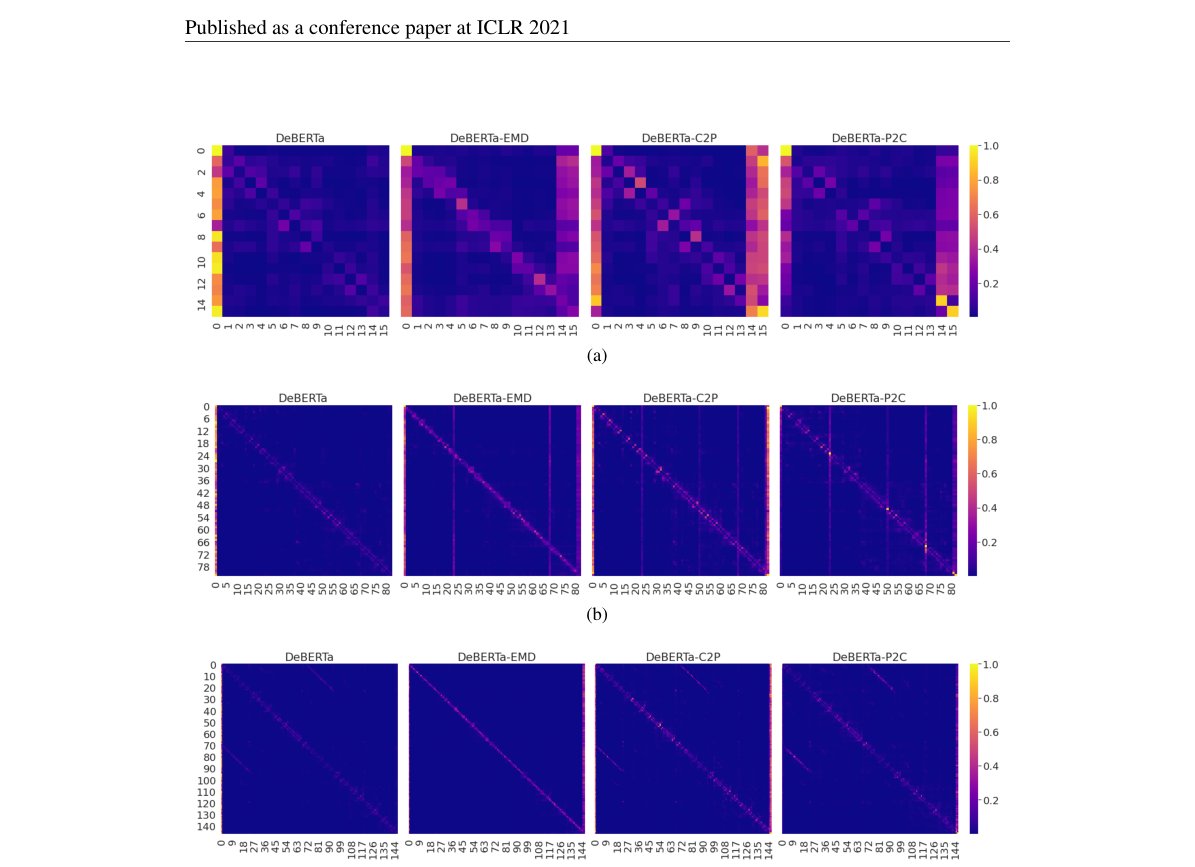
Figure 3: Comparison of attention patterns of the last layer among DeBERTa, RoBERTa and DeBERTa variants (i.e., DeBERTa without EMD, C2P and P2C respectively).
图 3:DeBERTa、RoBERTa 与 DeBERTa 变体(分别去掉 EMD、C2P 与 P2C)最后一层注意力模式对比。
To visualize how DeBERTa operates differently from RoBERTa, we present in Figure 3 the attention patterns (taken in the last self-attention layers) of RoBERTa, DeBERTa and three DeBERTa variants. We observe two differences. First, RoBERTa has a clear diagonal line effect for a token attending to itself. But this effect is not very visible in DeBERTa. This can be attributed to the use of EMD, in which the absolute position embedding is added to the hidden state of content as the query vector, as verified by the attention pattern of DeBERTa-EMD where the diagonal line effect is more visible than that of the original DeBERTa. Second, we observe vertical strips in the attention patterns of RoBERTa, which are mainly caused by high-frequent functional words or tokens (e.g., “a”, “the”, and punctuation). For DeBERTa, the strip only appears in the first column, which represents the [CLS] token. We conjecture that a dominant emphasis on [CLS] is desirable since the feature vector of [CLS] is often used as a contextual representation of the entire input sequence in downstream tasks. We also observe that the vertical strip effect is quite obvious in the patterns of the three DeBERTa variants.
为展示 DeBERTa 与 RoBERTa 运作上的差异,图 3 给出 RoBERTa、DeBERTa 及三个 DeBERTa 变体在最后自注意力层的注意力模式。我们观察到两点差异。第一,RoBERTa 中词元关注自身有清晰对角线效应,但在 DeBERTa 中不太明显。这可归因于使用 EMD:绝对位置嵌入加到内容隐状态上作为查询向量;去掉 EMD 的 DeBERTa-EMD 对角效应比原版 DeBERTa 更明显,可作印证。第二,RoBERTa 注意力模式中有竖条,主要来自高频功能词或标点(如 “a”、“the” 与标点)。DeBERTa 中竖条只出现在第一列,即 [CLS] 词元。我们推测对 [CLS] 的主导强调是可取的,因为下游任务常把 [CLS] 特征向量当作整段输入的上下文表示。三个 DeBERTa 变体的模式中竖条效应也相当明显。
We present three additional examples to illustrate the different attention patterns of DeBERTa and RoBERTa in Figures 4 and 5.
我们再给出三个例子,在图 4 与图 5 中说明 DeBERTa 与 RoBERTa 注意力模式的差异。
(a)
(a)
A.10 Account for the Variance in Fine-Tuning
A.10 考虑微调方差
Accounting for the variance of different runs of fine-tuning, in our experiments, we always follow (Liu et al., 2019c) to report the results on downstream tasks by averaging over five runs with different random initialization seeds, and perform significance test when comparing results. As the examples shown in Table 14, DeBERTabase significantly outperforms RoBERTabase (-value < 0.05).
考虑不同微调运行的方差,实验中我们始终沿用(Liu et al., 2019c),用五个不同随机初始化种子的平均结果报告下游任务表现,并在比较时做显著性检验。如表 14 示例,DeBERTabase 显著优于 RoBERTabase(-value < 0.05)。
| Model | MNLI-matched (Min/Max/Avg) | SQuAD v1.1 (Min/Max/Avg) | -value |
|---|---|---|---|
| RoBERTabase | 84.7/85.0/84.9 | 90.8/91.3/91.1 | 0.02 |
| DeBERTabase | 86.1/86.5/86.3 | 91.8/92.2/92.1 | 0.01 |
Table 14: Comparison of DeBERTa and RoBERTa on MNLI-matched and SQuAD v1.1.
| 模型 | MNLI-matched (Min/Max/Avg) | SQuAD v1.1 (Min/Max/Avg) | -value |
|---|---|---|---|
| RoBERTabase | 84.7/85.0/84.9 | 90.8/91.3/91.1 | 0.02 |
| DeBERTabase | 86.1/86.5/86.3 | 91.8/92.2/92.1 | 0.01 |
表 14:DeBERTa 与 RoBERTa 在 MNLI-matched 与 SQuAD v1.1 上的对比。
A.11 Further improve the model efficiency
A.11 进一步提升模型效率
In addition to scaling up transformer models with billions or trillions of parameters (Raffel et al., 2020; Brown et al., 2020; Fedus et al., 2021), it is important to improve model’s parameter efficiency (Kanakarajan et al., 2021). In A.3.1 we have shown that DeBERTa is more parameter efficient than BERT and RoBERTa. In this section, we show further improvements in terms of parameter efficiency.
除了把 Transformer 扩展到数十亿乃至数万亿参数(Raffel et al., 2020;Brown et al., 2020;Fedus et al., 2021),提升参数效率也很重要(Kanakarajan et al., 2021)。A.3.1 已表明 DeBERTa 比 BERT 与 RoBERTa 更参数高效。本节展示参数效率上的进一步改进。
Replaced token detection (RTD) is a new pre-training objective introduced by ELECTRA (Clark et al., 2020). It has been shown to be more effective than masked language model (MLM) (Devlin et al., 2019; Liu et al., 2019c). In DeBERTa, we replace the MLM objective with the RTD objective, and denote the new variant as DeBERTaRTD. We pre-train DeBERTaRTD using small, base and large settings with the same 160GB data as DeBERTa1.5B. Following (Meng et al., 2021), we set the width of the generator the same as that of the discriminator, but set its depth only half of the discriminator’s depth. Other hyper-parameters remain the same as DeBERTabase or DeBERTalarge. For the new member DeBERTa, it has 6 layers with the same width as DeBERTa. We evaluate our models on MNLI and SQuAD v2 datasets. Table 15 summarizes the results. We observe that both DeBERTa and DeBERTa significantly outperform other models. For example, DeBERTa obtains 0.9 absolute improvement over DeBERTaLarge (the previous SoTA model) on MNLI and SQuAD v2.0, respectively. It is worth noting that DeBERTa is on-par with DeBERTa1.5B while has only 1/3 parameters of DeBERTa1.5B. Furthermore, DeBERTa even outperforms BERTlarge by a large margin. All these demonstrate the efficiency of DeBERTaRTD models and clearly show a huge potential to further improve model’s parameter efficiency. Our work lays the base for future studies on far more parameter-efficient pre-trained language models.
替换词元检测(RTD)是 ELECTRA(Clark et al., 2020)引入的新预训练目标,已被证明比掩码语言模型(MLM)(Devlin et al., 2019;Liu et al., 2019c)更有效。在 DeBERTa 中我们用 RTD 替换 MLM,记新变体为 DeBERTaRTD。我们在 small、base 与 large 设定下用与 DeBERTa1.5B 相同的 160GB 数据预训练 DeBERTaRTD。沿用(Meng et al., 2021),生成器宽度与判别器相同,但深度仅为判别器一半。其余超参与 DeBERTabase 或 DeBERTalarge 相同。新成员 DeBERTa 有 6 层,宽度与 DeBERTa 相同。在 MNLI 与 SQuAD v2 上评测。表 15 汇总结果。可见 DeBERTa 与 DeBERTa 均显著优于其他模型。例如 DeBERTa 相对此前 SoTA 的 DeBERTaLarge,在 MNLI 与 SQuAD v2.0 上分别绝对提升 0.9。值得注意的是 DeBERTa 与 DeBERTa1.5B 相当,参数却只有后者的 1/3。此外 DeBERTa 甚至大幅超过 BERTlarge。这些都表明 DeBERTaRTD 的效率,并清楚显示进一步提升参数效率的巨大潜力。本工作为未来更参数高效的预训练语言模型研究打下基础。
| Model | MNLI(m/mm Acc) | SQuAD v2.0 (F1/EM) |
|---|---|---|
| BERT | 88.2/87.9 | 82.9/80.4 |
| BERTbase | 84.3/84.7 | 76.3/73.7 |
| RoBERTabase | 87.6/- | 83.7/80.5 |
| ELECTRAbase | 88.8/- | 83.3/80.5 |
| DeBERTabase | 88.8/88.5 | 86.2/83.1 |
| DeBERTa | 90.6/90.8 | 88.4/85.4 |
| BERTlarge | 86.6/- | 81.8/79.0 |
| RoBERTalarge | 90.2/90.2 | 89.4/86.5 |
| ELECTRAlarge | 90.9/- | 90.6/88.0 |
| DeBERTalarge | 91.1/91.1 | 90.7/88.0 |
| DeBERTa | 92.0/91.9 | 91.5/89.0 |
| DeBERTa1.5B | 91.7/91.9 | 92.2/89.7 |
Table 15: Comparison of different variants of DeBERTa models on MNLI and SQuAD 2.0.
| 模型 | MNLI(m/mm Acc) | SQuAD v2.0 (F1/EM) |
|---|---|---|
| BERT | 88.2/87.9 | 82.9/80.4 |
| BERTbase | 84.3/84.7 | 76.3/73.7 |
| RoBERTabase | 87.6/- | 83.7/80.5 |
| ELECTRAbase | 88.8/- | 83.3/80.5 |
| DeBERTabase | 88.8/88.5 | 86.2/83.1 |
| DeBERTa | 90.6/90.8 | 88.4/85.4 |
| BERTlarge | 86.6/- | 81.8/79.0 |
| RoBERTalarge | 90.2/90.2 | 89.4/86.5 |
| ELECTRAlarge | 90.9/- | 90.6/88.0 |
| DeBERTalarge | 91.1/91.1 | 90.7/88.0 |
| DeBERTa | 92.0/91.9 | 91.5/89.0 |
| DeBERTa1.5B | 91.7/91.9 | 92.2/89.7 |
表 15:不同 DeBERTa 变体在 MNLI 与 SQuAD 2.0 上的对比。