Deep Reinforcement Learning with Double Q-learning
Deep Reinforcement Learning with Double Q-learning
Hado van Hasselt Arthur Guez David Silver Affiliation: Google DeepMind
Abstract
摘要
The popular Q-learning algorithm is known to overestimate action values under certain conditions. It was not previously known whether, in practice, such overestimations are common, whether they harm performance, and whether they can generally be prevented. In this paper, we answer all these questions affirmatively. In particular, we first show that the recent DQN algorithm, which combines Q-learning with a deep neural network, suffers from substantial overestimations in some games in the Atari 2600 domain. We then show that the idea behind the Double Q-learning algorithm, which was introduced in a tabular setting, can be generalized to work with large-scale function approximation. We propose a specific adaptation to the DQN algorithm and show that the resulting algorithm not only reduces the observed overestimations, as hypothesized, but that this also leads to much better performance on several games.
流行的 Q-learning 算法在某些条件下会高估动作价值。此前并不清楚:实践中这种高估是否常见、是否损害表现、以及是否一般可被防止。本文对这三个问题都给出肯定回答。具体而言,我们首先表明:把 Q-learning 与深度网络结合的近期 DQN 算法,在 Atari 2600 若干游戏中存在显著高估。接着表明:在表格设定中提出的 Double Q-learning 思想,可推广到大规模函数近似。我们对 DQN 做了具体改编,并表明所得算法不仅如所假设地减少了观测到的高估,还在若干游戏上带来明显更好的表现。
The goal of reinforcement learning (Sutton and Barto 1998) is to learn good policies for sequential decision problems, by optimizing a cumulative future reward signal. Q-learning (Watkins 1989) is one of the most popular reinforcement learning algorithms, but it is known to sometimes learn unrealistically high action values because it includes a maximization step over estimated action values, which tends to prefer overestimated to underestimated values.
强化学习(Sutton and Barto 1998)的目标是通过优化累积未来奖励信号,为序列决策问题学习好策略。Q-learning(Watkins 1989)是最流行的强化学习算法之一,但有时会学到不切实际的高动作价值,因为它在估计的动作价值上包含最大化步骤,倾向于偏好高估而非低估的值。
In previous work, overestimations have been attributed to insufficiently flexible function approximation (Thrun and Schwartz 1993) and noise (van Hasselt 2010; van Hasselt 2011). In this paper, we unify these views and show overestimations can occur when the action values are inaccurate, irrespective of the source of approximation error. Of course, imprecise value estimates are the norm during learning, which indicates that overestimations may be much more common than previously appreciated.
既往工作把高估归因于不够灵活的函数近似(Thrun and Schwartz 1993)以及噪声(van Hasselt 2010;van Hasselt 2011)。本文统一这些观点,表明只要动作价值不准确——无论近似误差来源为何——都可能出现高估。当然,学习过程中价值估计不精确是常态,这意味着高估可能比以往认识的更为普遍。
It is an open question whether, if the overestimations do occur, this negatively affects performance in practice. Overoptimistic value estimates are not necessarily a problem in and of themselves. If all values would be uniformly higher then the relative action preferences are preserved and we would not expect the resulting policy to be any worse. Furthermore, it is known that sometimes it is good to be optimistic: optimism in the face of uncertainty is a well-known exploration technique (Kaelbling et al. 1996). If, however, the overestimations are not uniform and not concentrated at states about which we wish to learn more, then they might negatively affect the quality of the resulting policy. Thrun and Schwartz 1993 give specific examples in which this leads to suboptimal policies, even asymptotically.
若确有高估,是否会在实践中损害表现,仍是开放问题。价值估计偏乐观本身不一定成问题:若所有值统一偏高,相对动作偏好仍保留,所得策略未必更差。此外,有时乐观是有益的:面对不确定性保持乐观是著名的探索技术(Kaelbling et al. 1996)。然而,若高估并不均匀、也不集中在我们希望多学的状态上,就可能损害所得策略质量。Thrun and Schwartz 1993 给出了具体例子,说明这会导致次优策略,甚至渐近如此。
To test whether overestimations occur in practice and at scale, we investigate the performance of the recent DQN algorithm (Mnih et al. 2015). DQN combines Q-learning with a flexible deep neural network and was tested on a varied and large set of deterministic Atari 2600 games, reaching human-level performance on many games. In some ways, this setting is a best-case scenario for Q-learning, because the deep neural network provides flexible function approximation with the potential for a low asymptotic approximation error, and the determinism of the environments prevents the harmful effects of noise. Perhaps surprisingly, we show that even in this comparatively favorable setting DQN sometimes substantially overestimates the values of the actions.
为检验高估是否在实践中、在规模上发生,我们考察近期 DQN 算法(Mnih et al. 2015)。DQN 把 Q-learning 与灵活深度网络结合,并在多样的大规模确定性 Atari 2600 游戏上测试,许多游戏达到人类水平。在某些方面,这是 Q-learning 的最佳情形:深度网络提供灵活函数近似,有望实现较低渐近近似误差;环境确定性也避免了噪声的有害影响。或许出人意料,我们表明即便在这一相对有利设定下,DQN 有时仍大幅高估动作价值。
We show that the idea behind the Double Q-learning algorithm (van Hasselt 2010), which was first proposed in a tabular setting, can be generalized to work with arbitrary function approximation, including deep neural networks. We use this to construct a new algorithm we call Double DQN. We then show that this algorithm not only yields more accurate value estimates, but leads to much higher scores on several games. This demonstrates that the overestimations of DQN were indeed leading to poorer policies and that it is beneficial to reduce them. In addition, by improving upon DQN we obtain state-of-the-art results on the Atari domain.
我们表明:先在表格设定提出的 Double Q-learning(van Hasselt 2010)思想,可推广到任意函数近似(含深度网络)。据此构造称为 Double DQN 的新算法。接着表明该算法不仅给出更准的价值估计,还在若干游戏上取得高得多的分数。这说明 DQN 的高估确实导致更差策略,减少高估是有益的。此外,通过改进 DQN,我们在 Atari 领域取得了当时最优结果。
Background
背景
To solve sequential decision problems we can learn estimates for the optimal value of each action, defined as the expected sum of future rewards when taking that action and following the optimal policy thereafter. Under a given policy , the true value of an action in a state is
为求解序列决策问题,可学习各动作最优价值的估计,定义为采取该动作并此后遵循最优策略时未来奖励的期望和。在给定策略 下,状态 中动作 的真值为
where is a discount factor that trades off the importance of immediate and later rewards. The optimal value is then . An optimal policy is easily derived from the optimal values by selecting the highest-valued action in each state.
其中 为在即时与更远奖励之间权衡的折扣因子。最优价值则为 。最优策略可轻易从最优价值导出:在每个状态选择价值最高的动作。
Estimates for the optimal action values can be learned using Q-learning (Watkins 1989), a form of temporal difference learning (Sutton 1988). Most interesting problems are too large to learn all action values in all states separately. Instead, we can learn a parameterized value function . The standard Q-learning update for the parameters after taking action in state and observing the immediate reward and resulting state is then
最优动作价值的估计可用 Q-learning(Watkins 1989)学习,它是一种时序差分学习(Sutton 1988)。多数有趣问题过大,无法在所有状态分别学习所有动作价值。于是可学习参数化价值函数 。在状态 采取动作 、观测即时奖励 与下一状态 后,参数的标准 Q-learning 更新为
where is a scalar step size and the target is defined as
其中 为标量步长,目标 定义为
This update resembles stochastic gradient descent, updating the current value towards a target value .
该更新类似随机梯度下降,把当前值 朝目标值 推进。
Deep Q Networks
深度 Q 网络
A deep Q network (DQN) is a multi-layered neural network that for a given state outputs a vector of action values , where are the parameters of the network. For an -dimensional state space and an action space containing actions, the neural network is a function from to . Two important ingredients of the DQN algorithm as proposed by Mnih et al. 2015 are the use of a target network, and the use of experience replay. The target network, with parameters , is the same as the online network except that its parameters are copied every steps from the online network, so that then , and kept fixed on all other steps. The target used by DQN is then
深度 Q 网络(DQN)是多层神经网络:对给定状态 输出动作价值向量 ,其中 为网络参数。对 维状态空间与含 个动作的动作空间,网络是从 到 的函数。Mnih et al. 2015 提出的 DQN 算法有两个重要成分:目标网络与经验回放。目标网络参数为 ,与在线网络相同,只是每 步从在线网络复制参数(此时 ),其余步骤保持固定。DQN 使用的目标则为
For the experience replay (Lin 1992), observed transitions are stored for some time and sampled uniformly from this memory bank to update the network. Both the target network and the experience replay dramatically improve the performance of the algorithm (Mnih et al. 2015).
经验回放(Lin 1992)把观测到的转移存储一段时间,再从该记忆库均匀采样以更新网络。目标网络与经验回放都显著提升了算法表现(Mnih et al. 2015)。
Double Q-learning
The max operator in standard Q-learning and DQN, in (2) and (3), uses the same values both to select and to evaluate an action. This makes it more likely to select overestimated values, resulting in overoptimistic value estimates. To prevent this, we can decouple the selection from the evaluation. This is the idea behind Double Q-learning (van Hasselt 2010).
标准 Q-learning 与 DQN 中式 (2)(3) 的 max 算子用同一套价值既选择又评估动作。这更易选中被高估的值,导致价值估计偏乐观。为防止这一点,可将选择与评估解耦。这正是 Double Q-learning(van Hasselt 2010)背后的思想。
In the original Double Q-learning algorithm, two value functions are learned by assigning each experience randomly to update one of the two value functions, such that there are two sets of weights, and . For each update, one set of weights is used to determine the greedy policy and the other to determine its value. For a clear comparison, we can first untangle the selection and evaluation in Q-learning and rewrite its target (2) as
在原始 Double Q-learning 中,通过把每次经验随机分配去更新两个价值函数之一,学到两套权重 与 。每次更新时,一套权重决定贪心策略,另一套决定其价值。为便于对照,可先在 Q-learning 中拆开选择与评估,把目标 (2) 改写为
The Double Q-learning error can then be written as
于是 Double Q-learning 误差可写为
Notice that the selection of the action, in the , is still due to the online weights . This means that, as in Q-learning, we are still estimating the value of the greedy policy according to the current values, as defined by . However, we use the second set of weights to fairly evaluate the value of this policy. This second set of weights can be updated symmetrically by switching the roles of and .
注意 中的动作选择仍由在线权重 决定。这意味着与 Q-learning 一样,我们仍在按当前价值(由 定义)估计贪心策略的价值;但用第二套权重 公平评估该策略的价值。通过互换 与 的角色,可对称更新第二套权重。
Overoptimism due to estimation errors
由估计误差导致的过度乐观
Q-learning’s overestimations were first investigated by Thrun and Schwartz 1993, who showed that if the action values contain random errors uniformly distributed in an interval then each target is overestimated up to , where is the number of actions. In addition, Thrun and Schwartz 1993 give a concrete example in which these overestimations even asymptotically lead to sub-optimal policies, and show the overestimations manifest themselves in a small toy problem when using function approximation. Later van Hasselt 2010 argued that noise in the environment can lead to overestimations even when using tabular representation, and proposed Double Q-learning as a solution.
Q-learning 的高估最早由 Thrun and Schwartz 1993 研究:若动作价值含在区间 上均匀分布的随机误差,则每个目标至多被高估 ,其中 为动作数。此外他们给出具体例子,说明这些高估甚至渐近导致次优策略,并在小玩具问题上用函数近似展现高估。后来 van Hasselt 2010 主张:即便用表格表示,环境噪声也可导致高估,并提出 Double Q-learning 作为解法。
In this section we demonstrate more generally that estimation errors of any kind can induce an upward bias, regardless of whether these errors are due to environmental noise, function approximation, non-stationarity, or any other source. This is important, because in practice any method will incur some inaccuracies during learning, simply due to the fact that the true values are initially unknown.
本节更一般地表明:任何种类的估计误差都可诱导向上偏置,无论误差来自环境噪声、函数近似、非平稳还是其他来源。这很重要,因为实践中任何方法在学习过程中都会有不准确——仅仅因为真值起初未知。
The result by Thrun and Schwartz 1993 cited above gives an upper bound to the overestimation for a specific setup, but it is also possible, and potentially more interesting, to derive a lower bound.
上文引用的 Thrun and Schwartz 1993 结果给出特定设定下高估的上界;推导下界同样可能,且或许更有趣。
Theorem 1.
Consider a state in which all the true optimal action values are equal at $Q_{}(s,a)=V_{}(s)V_{}(s)Q_{t}\sum_{a}(Q_{t}(s,a)-V_{}(s))=0\frac{1}{m}\sum_{a}(Q_{t}(s,a)-V_{}(s))^{2}=CC>0m\geq 2s\max_{a}Q_{t}(s,a)\geq V_{}(s)+\sqrt{\frac{C}{m-1}}$. This lower bound is tight. Under the same conditions, the lower bound on the absolute error of the Double Q-learning estimate is zero. (Proof in appendix.)
定理 1。
考虑状态 ,其中所有真最优动作价值相等:$Q_{}(s,a)=V_{}(s)Q_{t}\sum_{a}(Q_{t}(s,a)-V_{}(s))=0\frac{1}{m}\sum_{a}(Q_{t}(s,a)-V_{}(s))^{2}=CC>0m\geq 2s\max_{a}Q_{t}(s,a)\geq V_{}(s)+\sqrt{\frac{C}{m-1}}$。该下界是紧的。在相同条件下,Double Q-learning 估计绝对误差的下界为零。(证明见附录。)*
Note that we did not need to assume that estimation errors for different actions are independent. This theorem shows that even if the value estimates are on average correct, estimation errors of any source can drive the estimates up and away from the true optimal values.
注意我们无需假设不同动作的估计误差独立。定理表明:即便价值估计平均正确,任意来源的估计误差仍可将估计推高并远离真最优价值。
The lower bound in Theorem 1 decreases with the number of actions. This is an artifact of considering the lower bound, which requires very specific values to be attained. More typically, the overoptimism increases with the number of actions as shown in Figure 1.
定理 1 的下界随动作数减小。这是考虑下界的产物,要求取到非常特定的值。更典型地,过度乐观随动作数增加,如图 1。
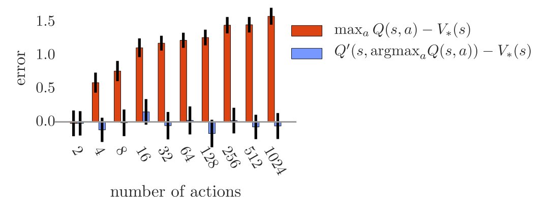
Figure 1: The orange bars show the bias in a single Q-learning update when the action values are and the errors are independent standard normal random variables. The second set of action values , used for the blue bars, was generated identically and independently. All bars are the average of 100 repetitions.
图 1:橙色柱表示单次 Q-learning 更新的偏置,此时动作价值为 ,误差 为独立标准正态随机变量。用于蓝色柱的第二套动作价值 以相同方式独立生成。所有柱为 100 次重复的平均。
Q-learning’s overestimations there indeed increase with the number of actions, while Double Q-learning is unbiased. As another example, if for all actions and the estimation errors are uniformly random in , then the overoptimism is . (Proof in appendix.)
可见 Q-learning 的高估确实随动作数增加,而 Double Q-learning 无偏。另一例:若对所有动作 ,且估计误差 在 上均匀随机,则过度乐观为 。(证明见附录。)
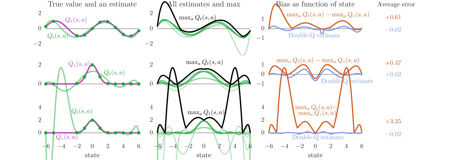
Figure 2: Illustration of overestimations during learning. In each state (x-axis), there are 10 actions. The left column shows the true values (purple line). All true action values are defined by . The green line shows estimated values for one action as a function of state, fitted to the true value at several sampled states (green dots). The middle column plots show all the estimated values (green), and the maximum of these values (dashed black). The maximum is higher than the true value (purple, left plot) almost everywhere. The right column plots shows the difference in orange. The blue line in the right plots is the estimate used by Double Q-learning with a second set of samples for each state. The blue line is much closer to zero, indicating less bias. The three rows correspond to different true functions (left, purple) or capacities of the fitted function (left, green). (Details in the text)
图 2:学习过程中高估的示意。每个状态(横轴)有 10 个动作。左列显示真值 (紫线)。所有真动作价值由 定义。绿线显示某一动作的估计值 作为状态的函数,拟合于若干采样状态上的真值(绿点)。中列画出所有估计值(绿)及其最大值(黑色虚线)。最大值几乎处处高于真值(左图紫线)。右列橙色为二者之差。右图蓝线是 Double Q-learning 用每状态第二套样本得到的估计,更接近零,表明偏置更小。三行对应不同真函数(左,紫)或拟合函数容量(左,绿)。(细节见正文)
We now turn to function approximation and consider a real-valued continuous state space with 10 discrete actions in each state. For simplicity, the true optimal action values in this example depend only on state so that in each state all actions have the same true value. These true values are shown in the left column of plots in Figure 2 (purple lines) and are defined as either (top row) or (middle and bottom rows). The left plots also show an approximation for a single action (green lines) as a function of state as well as the samples the estimate is based on (green dots). The estimate is a -degree polynomial that is fit to the true values at sampled states, where (top and middle rows) or (bottom row). The samples match the true function exactly: there is no noise and we assume we have ground truth for the action value on these sampled states. The approximation is inexact even on the sampled states for the top two rows because the function approximation is insufficiently flexible. In the bottom row, the function is flexible enough to fit the green dots, but this reduces the accuracy in unsampled states. Notice that the sampled states are spaced further apart near the left side of the left plots, resulting in larger estimation errors. In many ways this is a typical learning setting, where at each point in time we only have limited data.
我们转向函数近似,考虑实值连续状态空间,每状态 10 个离散动作。为简单起见,本例中真最优动作价值只依赖状态,因而每状态所有动作真值相同。这些真值见图 2 左列(紫线),定义为 (上行)或 (中、下行)。左图还显示单动作近似(绿线)及其所依据样本(绿点)。估计是拟合于采样状态真值的 次多项式,(上、中行)或 (下行)。样本精确匹配真函数:无噪声,并假设在这些采样状态上有动作价值的真值。上两行即便在采样状态上近似也不精确,因为函数近似不够灵活。下行函数灵活到足以拟合绿点,但这降低了未采样状态的精度。注意左图左侧采样状态间距更大,导致更大估计误差。这在许多方面是典型学习设定:任一时刻我们只有有限数据。
The middle column of plots in Figure 2 shows estimated action value functions for all 10 actions (green lines), as functions of state, along with the maximum action value in each state (black dashed line). Although the true value function is the same for all actions, the approximations differ because we have supplied different sets of sampled states.[^1] The maximum is often higher than the ground truth shown in purple on the left. This is confirmed in the right plots, which shows the difference between the black and purple curves in orange. The orange line is almost always positive, indicating an upward bias. The right plots also show the estimates from Double Q-learning in blue[^2], which are on average much closer to zero. This demonstrates that Double Q-learning indeed can successfully reduce the overoptimism of Q-learning.
图 2 中列显示全部 10 个动作的估计动作价值函数(绿线)随状态变化,以及每状态的最大动作价值(黑色虚线)。尽管所有动作的真价值函数相同,近似因我们提供了不同采样状态集而不同。[^1] 最大值常高于左侧紫色真值。右图确认这一点:橙色为黑线与紫线之差,几乎总为正,表明向上偏置。右图还显示 Double Q-learning 的蓝色估计[^2],平均更接近零。这表明 Double Q-learning 确实能成功降低 Q-learning 的过度乐观。
The different rows in Figure 2 show variations of the same experiment. The difference between the top and middle rows is the true value function, demonstrating that overestimations are not an artifact of a specific true value function. The difference between the middle and bottom rows is the flexibility of the function approximation. In the left-middle plot, the estimates are even incorrect for some of the sampled states because the function is insufficiently flexible. The function in the bottom-left plot is more flexible but this causes higher estimation errors for unseen states, resulting in higher overestimations. This is important because flexible parametric function approximators are often employed in reinforcement learning (see, e.g., Tesauro 1995; Sallans and Hinton 2004; Riedmiller 2005; Mnih et al. 2015).
图 2 不同行是同一实验的变体。上、中行差别在真价值函数,说明高估不是特定真函数的产物。中、下行差别在函数近似的灵活性。左中图中,因函数不够灵活,部分采样状态上的估计甚至不正确。左下图函数更灵活,却导致未见状态上更高估计误差,从而更高高估。这很重要,因为强化学习常采用灵活参数函数近似器(参见 Tesauro 1995;Sallans and Hinton 2004;Riedmiller 2005;Mnih et al. 2015)。
In contrast to van Hasselt 2010 we did not use a statistical argument to find overestimations, the process to obtain Figure 2 is fully deterministic. In contrast to Thrun and Schwartz 1993, we did not rely on inflexible function approximation with irreducible asymptotic errors; the bottom row shows that a function that is flexible enough to cover all samples leads to high overestimations. This indicates that the overestimations can occur quite generally.
与 van Hasselt 2010 不同,我们未用统计论证发现高估,得到图 2 的过程完全确定。与 Thrun and Schwartz 1993 不同,我们未依赖带不可约渐近误差的不灵活函数近似;下行表明足以覆盖所有样本的灵活函数仍导致高高估。这说明高估可相当普遍地发生。
In the examples above, overestimations occur even when assuming we have samples of the true action value at certain states. The value estimates can further deteriorate if we bootstrap off of action values that are already overoptimistic, since this causes overestimations to propagate throughout our estimates. Although uniformly overestimating values might not hurt the resulting policy, in practice overestimation errors will differ for different states and actions. Overestimation combined with bootstrapping then has the pernicious effect of propagating the wrong relative information about which states are more valuable than others, directly affecting the quality of the learned policies.
上例中,即便假设在某些状态有真动作价值样本,仍出现高估。若我们自举已过度乐观的动作价值,估计会进一步恶化,因为高估会在估计中传播。虽然均匀高估可能不伤所得策略,实践中不同状态与动作的高估误差会不同。高估与自举结合后,有害效果是传播关于哪些状态更有价值的错误相对信息,直接损害所学策略质量。
The overestimations should not be confused with optimism in the face of uncertainty (Sutton 1990; Agrawal 1995; Kaelbling et al. 1996; Auer et al. 2002; Brafman and Tennenholtz 2003; Szita and Lőrincz 2008; Strehl et al. 2009), where an exploration bonus is given to states or actions with uncertain values. Conversely, the overestimations discussed here occur only after updating, resulting in overoptimism in the face of apparent certainty. This was already observed by Thrun and Schwartz 1993, who noted that, in contrast to optimism in the face of uncertainty, these overestimations actually can impede learning an optimal policy. We will see this negative effect on policy quality confirmed later in the experiments as well: when we reduce the overestimations using Double Q-learning, the policies improve.
这些高估不应与面对不确定性的乐观混淆(Sutton 1990;Agrawal 1995;Kaelbling et al. 1996;Auer et al. 2002;Brafman and Tennenholtz 2003;Szita and Lőrincz 2008;Strehl et al. 2009)——后者给价值不确定的状态或动作探索奖励。相反,这里讨论的高估只在更新之后出现,表现为面对表面确定性时的过度乐观。Thrun and Schwartz 1993 已观察到:与面对不确定性的乐观相反,这些高估实际上会阻碍学习最优策略。后文实验也会确认对策略质量的负面影响:用 Double Q-learning 降低高估后,策略得到改进。
Double DQN
The idea of Double Q-learning is to reduce overestimations by decomposing the max operation in the target into action selection and action evaluation. Although not fully decoupled, the target network in the DQN architecture provides a natural candidate for the second value function, without having to introduce additional networks. We therefore propose to evaluate the greedy policy according to the online network, but using the target network to estimate its value. In reference to both Double Q-learning and DQN, we refer to the resulting algorithm as Double DQN. Its update is the same as for DQN, but replacing the target with
Double Q-learning 的思想是把目标中的 max 运算拆成动作选择与动作评估,以降低高估。虽未完全解耦,DQN 结构中的目标网络为第二价值函数提供了自然候选,无需引入额外网络。因此我们提出:按在线网络评估贪心策略,但用目标网络估计其价值。兼顾 Double Q-learning 与 DQN,称所得算法为 Double DQN。其更新与 DQN 相同,只是把目标 换成
In comparison to Double Q-learning (4), the weights of the second network are replaced with the weights of the target network for the evaluation of the current greedy policy. The update to the target network stays unchanged from DQN, and remains a periodic copy of the online network.
相对 Double Q-learning (4),评估当前贪心策略时,第二网络权重 换成目标网络权重 。目标网络的更新方式与 DQN 相同,仍是在线网络的周期性拷贝。
This version of Double DQN is perhaps the minimal possible change to DQN towards Double Q-learning. The goal is to get most of the benefit of Double Q-learning, while keeping the rest of the DQN algorithm intact for a fair comparison, and with minimal computational overhead.
该版 Double DQN 或许是把 DQN 推向 Double Q-learning 的最小改动。目标是在尽量保持 DQN 其余部分不变以便公平比较、且计算开销最小的前提下,拿到 Double Q-learning 的大部分收益。
Empirical results
经验结果
In this section, we analyze the overestimations of DQN and show that Double DQN improves over DQN both in terms of value accuracy and in terms of policy quality. To further test the robustness of the approach we additionally evaluate the algorithms with random starts generated from expert human trajectories, as proposed by Nair et al. 2015.
本节分析 DQN 的高估,并表明 Double DQN 在价值准确性与策略质量两方面都优于 DQN。为进一步检验方法稳健性,我们还按 Nair et al. 2015 的提议,用专家人类轨迹生成的随机起点评估算法。
Our testbed consists of Atari 2600 games, using the Arcade Learning Environment (Bellemare et al. 2013). The goal is for a single algorithm, with a fixed set of hyperparameters, to learn to play each of the games separately from interaction given only the screen pixels as input. This is a demanding testbed: not only are the inputs high-dimensional, the game visuals and game mechanics vary substantially between games. Good solutions must therefore rely heavily on the learning algorithm — it is not practically feasible to overfit the domain by relying only on tuning.
测试床为 Atari 2600 游戏,使用 Arcade Learning Environment(Bellemare et al. 2013)。目标是:单一算法、固定超参数,仅以屏幕像素为输入,通过交互分别学会玩每款游戏。这是苛刻的测试床:输入高维,且游戏画面与机制在游戏间差异很大。好的解法因此必须重度依赖学习算法——仅靠调参过拟合该领域在实践上不可行。
We closely follow the experimental setting and network architecture outlined by Mnih et al. 2015. Briefly, the network architecture is a convolutional neural network (Fukushima 1988; LeCun et al. 1998) with 3 convolution layers and a fully-connected hidden layer (approximately 1.5M parameters in total). The network takes the last four frames as input and outputs the action value of each action. On each game, the network is trained on a single GPU for 200M frames, or approximately 1 week.
我们紧密遵循 Mnih et al. 2015 的实验设定与网络结构。简言之,网络是含 3 个卷积层与一个全连接隐层的卷积神经网络(Fukushima 1988;LeCun et al. 1998)(共约 150 万参数)。网络以最近四帧为输入,输出每个动作的动作价值。每款游戏在单块 GPU 上训练 2 亿帧,约一周。
Results on overoptimism
关于过度乐观的结果
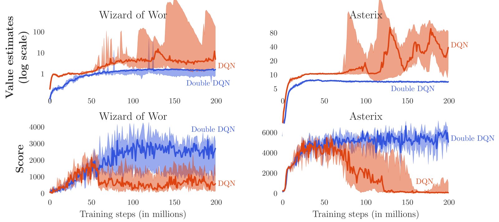
Figure 3: The top and middle rows show value estimates by DQN (orange) and Double DQN (blue) on six Atari games. The results are obtained by running DQN and Double DQN with 6 different random seeds with the hyper-parameters employed by Mnih et al. 2015. The darker line shows the median over seeds and we average the two extreme values to obtain the shaded area (i.e., 10% and 90% quantiles with linear interpolation). The straight horizontal orange (for DQN) and blue (for Double DQN) lines in the top row are computed by running the corresponding agents after learning concluded, and averaging the actual discounted return obtained from each visited state. These straight lines would match the learning curves at the right side of the plots if there is no bias. The middle row shows the value estimates (in log scale) for two games in which DQN’s overoptimism is quite extreme. The bottom row shows the detrimental effect of this on the score achieved by the agent as it is evaluated during training: the scores drop when the overestimations begin. Learning with Double DQN is much more stable.
图 3:上、中行显示 DQN(橙)与 Double DQN(蓝)在六款 Atari 游戏上的价值估计。结果由使用 Mnih et al. 2015 超参数、6 个不同随机种子运行 DQN 与 Double DQN 得到。深色线为多种子中位数;阴影为两个极值的平均(即带线性插值的 10% 与 90% 分位数)。上行中橙色(DQN)与蓝色(Double DQN)水平直线:学习结束后运行对应智能体,并对每个访问状态的实际折扣回报取平均。若无偏置,这些直线应与曲线右侧吻合。中行以对数尺度显示两款游戏上 DQN 过度乐观极为极端时的价值估计。下行显示这对训练中评估得分的有害影响:高估开始时分数下降。用 Double DQN 学习稳定得多。
Figure 3 shows examples of DQN’s overestimations in six Atari games. DQN and Double DQN were both trained under the exact conditions described by Mnih et al. 2015. DQN is consistently and sometimes vastly overoptimistic about the value of the current greedy policy, as can be seen by comparing the orange learning curves in the top row of plots to the straight orange lines, which represent the actual discounted value of the best learned policy. More precisely, the (averaged) value estimates are computed regularly during training with full evaluation phases of length steps as
图 3 给出六款 Atari 游戏上 DQN 高估的例子。DQN 与 Double DQN 均在 Mnih et al. 2015 描述的精确条件下训练。通过比较上行橙色学习曲线与表示最佳所学策略实际折扣价值的橙色水平线可见:DQN 对当前贪心策略价值持续、有时极度乐观。更精确地说,在训练过程中定期用长度 步的完整评估阶段计算(平均)价值估计为
The ground truth averaged values are obtained by running the best learned policies for several episodes and computing the actual cumulative rewards. Without overestimations we would expect these quantities to match up (i.e., the curve to match the straight line at the right of each plot). Instead, the learning curves of DQN consistently end up much higher than the true values. The learning curves for Double DQN, shown in blue, are much closer to the blue straight line representing the true value of the final policy. Note that the blue straight line is often higher than the orange straight line. This indicates that Double DQN does not just produce more accurate value estimates but also better policies.
真值平均价值通过运行最佳所学策略若干回合并计算实际累积奖励得到。若无高估,我们期望这些量吻合(即曲线在每图右侧与水平线重合)。相反,DQN 学习曲线终点 始终远高于真值。蓝色 Double DQN 学习曲线更接近表示最终策略真值的蓝色水平线。注意蓝水平线常高于橙水平线,说明 Double DQN 不仅给出更准的价值估计,也给出更好策略。
More extreme overestimations are shown in the middle two plots, where DQN is highly unstable on the games Asterix and Wizard of Wor. Notice the log scale for the values on the -axis. The bottom two plots shows the corresponding scores for these two games. Notice that the increases in value estimates for DQN in the middle plots coincide with decreasing scores in bottom plots. Again, this indicates that the overestimations are harming the quality of the resulting policies. If seen in isolation, one might perhaps be tempted to think the observed instability is related to inherent instability problems of off-policy learning with function approximation (Baird 1995; Tsitsiklis and Van Roy 1997; Sutton et al. 2008; Maei 2011; Sutton et al. 2015). However, we see that learning is much more stable with Double DQN, suggesting that the cause for these instabilities is in fact Q-learning’s overoptimism. Figure 3 only shows a few examples, but overestimations were observed for DQN in all 49 tested Atari games, albeit in varying amounts.
中两图显示更极端的高估:DQN 在 Asterix 与 Wizard of Wor 上高度不稳定。注意 轴价值为对数尺度。下两图为这两款游戏的对应分数。注意中图 DQN 价值估计上升与下图分数下降同时发生,再次表明高估损害所得策略质量。若孤立来看,或易把观测到的不稳定归因于带函数近似的离策略学习固有不稳定性(Baird 1995;Tsitsiklis and Van Roy 1997;Sutton et al. 2008;Maei 2011;Sutton et al. 2015)。但我们看到 Double DQN 学习稳定得多,说明这些不稳定的原因其实是 Q-learning 的过度乐观。图 3 只展示若干例子,但在全部 49 款测试的 Atari 游戏上均观测到 DQN 高估,程度各异。
Quality of the learned policies
所学策略质量
| DQN | Double DQN | |
|---|---|---|
| Median | 93.5% | 114.7% |
| Mean | 241.1% | 330.3% |
Table 1: Summary of normalized performance up to 5 minutes of play on 49 games. Results for DQN are from Mnih et al. 2015
| DQN | Double DQN | |
|---|---|---|
| Median | 93.5% | 114.7% |
| Mean | 241.1% | 330.3% |
表 1:在 49 款游戏上最多 5 分钟对局的归一化表现汇总。DQN 结果来自 Mnih et al. 2015。
Overoptimism does not always adversely affect the quality of the learned policy. For example, DQN achieves optimal behavior in Pong despite slightly overestimating the policy value. Nevertheless, reducing overestimations can significantly benefit the stability of learning; we see clear examples of this in Figure 3. We now assess more generally how much Double DQN helps in terms of policy quality by evaluating on all 49 games that DQN was tested on.
过度乐观并不总是损害所学策略质量。例如,DQN 在 Pong 上虽略微高估策略价值,仍达到最优行为。尽管如此,减少高估可显著提升学习稳定性;图 3 已给出清晰例子。我们现更系统地评估 Double DQN 对策略质量的帮助,在 DQN 曾测试的全部 49 款游戏上评测。
As described by Mnih et al. 2015 each evaluation episode starts by executing a special no-op action that does not affect the environment up to 30 times, to provide different starting points for the agent. Some exploration during evaluation provides additional randomization. For Double DQN we used the exact same hyper-parameters as for DQN, to allow for a controlled experiment focused just on reducing overestimations. The learned policies are evaluated for 5 mins of emulator time (18,000 frames) with an -greedy policy where . The scores are averaged over 100 episodes. The only difference between Double DQN and DQN is the target, using rather than . This evaluation is somewhat adversarial, as the used hyper-parameters were tuned for DQN but not for Double DQN.
按 Mnih et al. 2015 的描述,每轮评估开始时执行最多 30 次不影响环境的特殊空操作,为智能体提供不同起点。评估中的少量探索提供额外随机化。对 Double DQN,我们使用与 DQN 完全相同的超参数,以便对照实验只聚焦于减少高估。所学策略用 -贪心策略()评估 5 分钟模拟器时间(18,000 帧)。分数在 100 个回合上取平均。Double DQN 与 DQN 的唯一差别是目标:使用 而非 。该评估在某种程度上对 Double DQN 不利,因为所用超参数为 DQN 调优,而非为 Double DQN。
To obtain summary statistics across games, we normalize the score for each game as follows:
为得到跨游戏的汇总统计,按下式归一化每款游戏的分数:
The ‘random’ and ‘human’ scores are the same as used by Mnih et al. 2015, and are given in the appendix.
「随机」与「人类」分数与 Mnih et al. 2015 相同,见附录。
Table 1, under no ops, shows that on the whole Double DQN clearly improves over DQN. A detailed comparison (in appendix) shows that there are several games in which Double DQN greatly improves upon DQN. Noteworthy examples include Road Runner (from 233% to 617%), Asterix (from 70% to 180%), Zaxxon (from 54% to 111%), and Double Dunk (from 17% to 397%).
表 1 在 无空操作 设定下表明:总体而言 Double DQN 明显优于 DQN。附录中的细项对比显示,若干游戏上 Double DQN 相对 DQN 大幅提升。突出例子包括 Road Runner(从 233% 到 617%)、Asterix(从 70% 到 180%)、Zaxxon(从 54% 到 111%)以及 Double Dunk(从 17% 到 397%)。
The Gorila algorithm (Nair et al. 2015), which is a massively distributed version of DQN, is not included in the table because the architecture and infrastructure is sufficiently different to make a direct comparison unclear. For completeness, we note that Gorila obtained median and mean normalized scores of 96% and 495%, respectively.
Gorila 算法(Nair et al. 2015)是大规模分布式版 DQN,因其结构与基础设施差异过大,不宜直接对比,故未列入表中。为完整起见,我们注明 Gorila 的中位数与均值归一化得分分别为 96% 与 495%。
Robustness to Human starts
对人类起点的稳健性
| DQN | Double DQN | Double DQN (tuned) | |
|---|---|---|---|
| Median | 47.5% | 88.4% | 116.7% |
| Mean | 122.0% | 273.1% | 475.2% |
Table 2: Summary of normalized performance up to 30 minutes of play on 49 games with human starts. Results for DQN are from Nair et al. 2015.
| DQN | Double DQN | Double DQN (tuned) | |
|---|---|---|---|
| Median | 47.5% | 88.4% | 116.7% |
| Mean | 122.0% | 273.1% | 475.2% |
表 2:在 49 款游戏上、人类起点、最多 30 分钟对局的归一化表现汇总。DQN 结果来自 Nair et al. 2015。
One concern with the previous evaluation is that in deterministic games with a unique starting point the learner could potentially learn to remember sequences of actions without much need to generalize. While successful, the solution would not be particularly robust. By testing the agents from various starting points, we can test whether the found solutions generalize well, and as such provide a challenging testbed for the learned polices (Nair et al. 2015).
前述评估的一个顾虑是:在起点唯一的确定性游戏中,学习器可能主要靠记住动作序列,而不太需要泛化。尽管成功,这种解法并不稳健。通过在多种起点上测试智能体,可以检验所得解是否泛化良好,从而为所学策略提供更具挑战性的测试床(Nair et al. 2015)。
We obtained 100 starting points sampled for each game from a human expert’s trajectory, as proposed by Nair et al. 2015. We start an evaluation episode from each of these starting points and run the emulator for up to 108,000 frames (30 mins at 60Hz including the trajectory before the starting point). Each agent is only evaluated on the rewards accumulated after the starting point.
按 Nair et al. 2015 的提议,我们从人类专家轨迹中为每款游戏采样 100 个起点。从每个起点开始一局评估,模拟器最多运行 108,000 帧(60Hz 下 30 分钟,含起点前的轨迹)。每个智能体只按其起点之后累积的奖励计分。
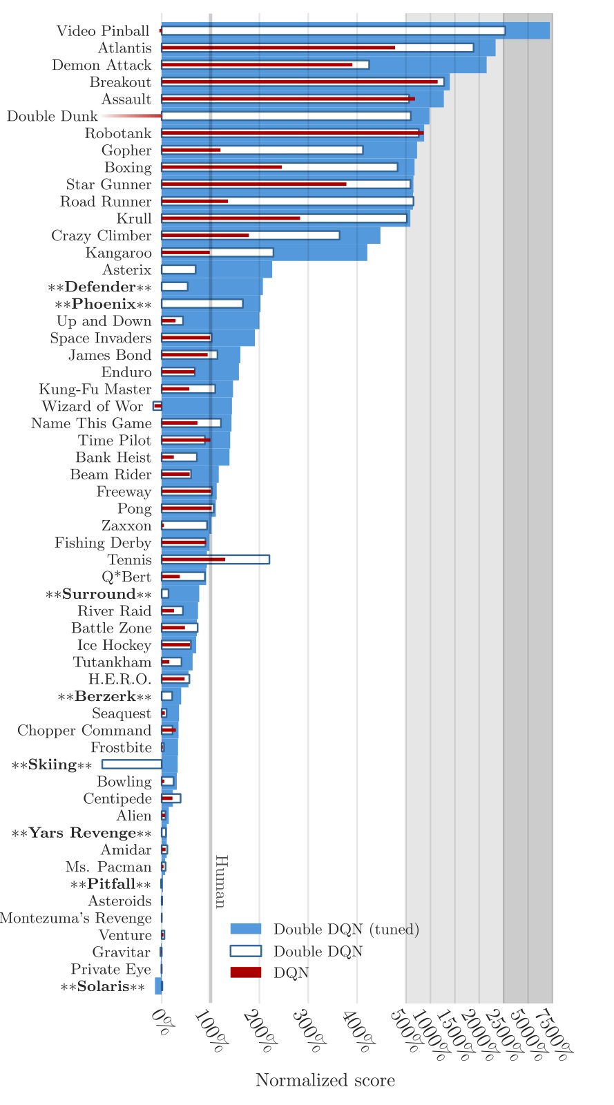
Figure 4: Normalized scores on 57 Atari games, tested for 100 episodes per game with human starts. Compared to Mnih et al. 2015, eight games additional games were tested. These are indicated with stars and a bold font.
图 4:在 57 款 Atari 游戏上的归一化得分,每款游戏用人类起点测试 100 个回合。相对 Mnih et al. 2015,另测了 8 款游戏;图中用星号与粗体标出。
For this evaluation we include a tuned version of Double DQN. Some tuning is appropriate because the hyperparameters were tuned for DQN, which is a different algorithm. For the tuned version of Double DQN, we increased the number of frames between each two copies of the target network from 10,000 to 30,000, to reduce overestimations further because immediately after each switch DQN and Double DQN both revert to Q-learning. In addition, we reduced the exploration during learning from to , and then used during evaluation. Finally, the tuned version uses a single shared bias for all action values in the top layer of the network. Each of these changes improved performance and together they result in clearly better results.[^3]
本评估中我们加入调优版 Double DQN。适当调参是合理的,因为原超参数是为另一算法 DQN 调的。调优版把两次目标网络拷贝之间的帧数从 10,000 提到 30,000,以进一步降低高估——每次切换后 DQN 与 Double DQN 都会暂时退回 Q-learning。此外,学习时探索从 降到 ,评估时用 。最后,调优版在网络顶层对所有动作价值使用单一共享偏置。每一项改动都提升了表现,合在一起结果明显更好。[^3]
Table 2 reports summary statistics for this evaluation on the 49 games from Mnih et al. 2015. Double DQN obtains clearly higher median and mean scores. Again Gorila DQN (Nair et al. 2015) is not included in the table, but for completeness note it obtained a median of 78% and a mean of 259%. Detailed results, plus results for an additional 8 games, are available in Figure 4 and in the appendix. On several games the improvements from DQN to Double DQN are striking, in some cases bringing scores much closer to human, or even surpassing these.
表 2 报告了在 Mnih et al. 2015 的 49 款游戏上该评估的汇总统计。Double DQN 的中位数与均值得分明显更高。Gorila DQN(Nair et al. 2015)仍未列入表中,但为完整起见注明其中位数 78%、均值 259%。细项结果以及额外 8 款游戏见图 4 与附录。若干游戏上从 DQN 到 Double DQN 的提升十分显著,有时把分数拉近甚至超过人类水平。
Double DQN appears more robust to this more challenging evaluation, suggesting that appropriate generalizations occur and that the found solutions do not exploit the determinism of the environments. This is appealing, as it indicates progress towards finding general solutions rather than a deterministic sequence of steps that would be less robust.
Double DQN 在这一更具挑战的评估上显得更稳健,说明发生了恰当的泛化,所得解并未利用环境的确定性。这一点很有吸引力:它表明我们在朝找一般解前进,而不是学一套不够稳健的确定性步骤序列。
Discussion
讨论
This paper has five contributions. First, we have shown why Q-learning can be overoptimistic in large-scale problems, even if these are deterministic, due to the inherent estimation errors of learning. Second, by analyzing the value estimates on Atari games we have shown that these overestimations are more common and severe in practice than previously acknowledged. Third, we have shown that Double Q-learning can be used at scale to successfully reduce this overoptimism, resulting in more stable and reliable learning. Fourth, we have proposed a specific implementation called Double DQN, that uses the existing architecture and deep neural network of the DQN algorithm without requiring additional networks or parameters. Finally, we have shown that Double DQN finds better policies, obtaining new state-of-the-art results on the Atari 2600 domain.
本文有五点贡献。第一,我们说明了即便问题确定,Q-learning 仍可因学习固有的估计误差在大规模问题上过度乐观。第二,通过分析 Atari 游戏上的价值估计,表明这些高估在实践中比以往认识的更普遍、更严重。第三,我们表明 Double Q-learning 可规模化使用,成功降低过度乐观,使学习更稳定可靠。第四,我们提出名为 Double DQN 的具体实现:沿用 DQN 的既有结构与深度网络,无需额外网络或参数。第五,我们表明 Double DQN 找到更好策略,在 Atari 2600 领域取得新的当时最优结果。
Acknowledgments
We would like to thank Tom Schaul, Volodymyr Mnih, Marc Bellemare, Thomas Degris, Georg Ostrovski, and Richard Sutton for helpful comments, and everyone at Google DeepMind for a constructive research environment.
References
Agrawal (1995) R. Agrawal. Sample mean based index policies with O(log n) regret for the multi-armed bandit problem. Advances in Applied Probability , pages 1054–1078, 1995.
Auer et al. (2002) P. Auer, N. Cesa-Bianchi, and P. Fischer. Finite-time analysis of the multiarmed bandit problem. Machine learning , 47(2-3):235–256, 2002.
Baird (1995) L. Baird. Residual algorithms: Reinforcement learning with function approximation. In Machine Learning: Proceedings of the Twelfth International Conference , pages 30–37, 1995.
Bellemare et al. (2013) M. G. Bellemare, Y. Naddaf, J. Veness, and M. Bowling. The arcade learning environment: An evaluation platform for general agents. J. Artif. Intell. Res. (JAIR) , 47:253–279, 2013.
Brafman and Tennenholtz (2003) R. I. Brafman and M. Tennenholtz. R-max-a general polynomial time algorithm for near-optimal reinforcement learning. The Journal of Machine Learning Research , 3:213–231, 2003.
Fukushima (1988) K. Fukushima. Neocognitron: A hierarchical neural network capable of visual pattern recognition. Neural networks , 1(2):119–130, 1988.
Kaelbling et al. (1996) L. P. Kaelbling, M. L. Littman, and A. W. Moore. Reinforcement learning: A survey. Journal of Artificial Intelligence Research , 4:237–285, 1996.
LeCun et al. (1998) Y. LeCun, L. Bottou, Y. Bengio, and P. Haffner. Gradient-based learning applied to document recognition. Proceedings of the IEEE , 86(11):2278–2324, 1998.
Lin (1992) L. Lin. Self-improving reactive agents based on reinforcement learning, planning and teaching. Machine learning , 8(3):293–321, 1992.
Maei (2011) H. R. Maei. Gradient temporal-difference learning algorithms . PhD thesis, University of Alberta, 2011.
Mnih et al. (2015) V. Mnih, K. Kavukcuoglu, D. Silver, A. A. Rusu, J. Veness, M. G. Bellemare, A. Graves, M. Riedmiller, A. K. Fidjeland, G. Ostrovski, S. Petersen, C. Beattie, A. Sadik, I. Antonoglou, H. King, D. Kumaran, D. Wierstra, S. Legg, and D. Hassabis. Human-level control through deep reinforcement learning. Nature , 518(7540):529–533, 2015.
Nair et al. (2015) A. Nair, P. Srinivasan, S. Blackwell, C. Alcicek, R. Fearon, A. D. Maria, V. Panneershelvam, M. Suleyman, C. Beattie, S. Petersen, S. Legg, V. Mnih, K. Kavukcuoglu, and D. Silver. Massively parallel methods for deep reinforcement learning. In Deep Learning Workshop, ICML , 2015.
Riedmiller (2005) M. Riedmiller. Neural fitted Q iteration - first experiences with a data efficient neural reinforcement learning method. In J. Gama, R. Camacho, P. Brazdil, A. Jorge, and L. Torgo, editors, Proceedings of the 16th European Conference on Machine Learning (ECML’05) , pages 317–328. Springer, 2005.
Sallans and Hinton (2004) B. Sallans and G. E. Hinton. Reinforcement learning with factored states and actions. The Journal of Machine Learning Research , 5:1063–1088, 2004.
Strehl et al. (2009) A. L. Strehl, L. Li, and M. L. Littman. Reinforcement learning in finite MDPs: PAC analysis. The Journal of Machine Learning Research , 10:2413–2444, 2009.
Sutton (1988) R. S. Sutton. Learning to predict by the methods of temporal differences. Machine learning , 3(1):9–44, 1988.
Sutton (1990) R. S. Sutton. Integrated architectures for learning, planning, and reacting based on approximating dynamic programming. In Proceedings of the seventh international conference on machine learning , pages 216–224, 1990.
Sutton and Barto (1998) R. S. Sutton and A. G. Barto. Introduction to reinforcement learning . MIT Press, 1998.
Sutton et al. (2008) R. S. Sutton, C. Szepesvári, and H. R. Maei. A convergent O(n) algorithm for off-policy temporal-difference learning with linear function approximation. Advances in Neural Information Processing Systems 21 (NIPS-08) , 21:1609–1616, 2008.
Sutton et al. (2015) R. S. Sutton, A. R. Mahmood, and M. White. An emphatic approach to the problem of off-policy temporal-difference learning. arXiv preprint arXiv:1503.04269 , 2015.
Szita and Lőrincz (2008) I. Szita and A. Lőrincz. The many faces of optimism: a unifying approach. In Proceedings of the 25th international conference on Machine learning , pages 1048–1055. ACM, 2008.
Tesauro (1995) G. Tesauro. Temporal difference learning and td-gammon. Communications of the ACM , 38(3):58–68, 1995.
Thrun and Schwartz (1993) S. Thrun and A. Schwartz. Issues in using function approximation for reinforcement learning. In M. Mozer, P. Smolensky, D. Touretzky, J. Elman, and A. Weigend, editors, Proceedings of the 1993 Connectionist Models Summer School , Hillsdale, NJ, 1993. Lawrence Erlbaum.
Tsitsiklis and Van Roy (1997) J. N. Tsitsiklis and B. Van Roy. An analysis of temporal-difference learning with function approximation. IEEE Transactions on Automatic Control , 42(5):674–690, 1997.
van Hasselt (2010) H. van Hasselt. Double Q-learning. Advances in Neural Information Processing Systems , 23:2613–2621, 2010.
van Hasselt (2011) H. van Hasselt. Insights in Reinforcement Learning . PhD thesis, Utrecht University, 2011.
Watkins (1989) C. J. C. H. Watkins. Learning from delayed rewards . PhD thesis, University of Cambridge England, 1989.
Appendix
附录
Theorem 1.
Consider a state in which all the true optimal action values are equal at $Q_{}(s,a)=V_{}(s)V_{}(s)Q_{t}\sum_{a}(Q_{t}(s,a)-V_{}(s))=0\frac{1}{m}\sum_{a}(Q_{t}(s,a)-V_{}(s))^{2}=CC>0m\geq 2s\max_{a}Q_{t}(s,a)\geq V_{}(s)+\sqrt{\frac{C}{m-1}}$. This lower bound is tight. Under the same conditions, the lower bound on the absolute error of the Double Q-learning estimate is zero.
Theorem 1.
考虑状态 ,其中所有真最优动作价值相等:$Q_{}(s,a)=V_{}(s)V_{}(s)Q_{t}\sum_{a}(Q_{t}(s,a)-V_{}(s))=0\frac{1}{m}\sum_{a}(Q_{t}(s,a)-V_{}(s))^{2}=CC>0m\geq 2s\max_{a}Q_{t}(s,a)\geq V_{}(s)+\sqrt{\frac{C}{m-1}}$。该下界是紧的。在相同条件下,Double Q-learning 估计绝对误差的下界为零。
Proof of Theorem 1.
Define the errors for each action as . Suppose that there exists a setting of such that . Let be the set of positive of size , and the set of strictly negative of size (such that ). If , then , which contradicts . Hence, it must be that . Then, , and therefore (using the constraint ) we also have that . This implies . By Hölder’s inequality, then
定理 1 的证明。
定义各动作 的误差为 。假设存在一组 使 。令 为正误差集合,大小为 ; 为严格负误差集合,大小为 (因而 )。若 ,则 ,与 矛盾。故必有 。于是 ,再利用约束 ,亦有 。由此 。由 Hölder 不等式,
We can now combine these relations to compute an upper-bound on the sum of squares for all :
现可合并这些关系,得到全体 平方和的上界:
This contradicts the assumption that , and therefore for all settings of that satisfy the constraints. We can check that the lower-bound is tight by setting for and . This verifies and .
这与假设 矛盾,因此对所有满足约束的 设定,均有 。可取 ()且 验证下界紧:此时 且 。
The only tight lower bound on the absolute error for Double Q-learning is zero. This can be seen by because we can have
对 Double Q-learning, 的唯一紧下界为零。这是因为可以取
and
以及
Then the conditions of the theorem hold. If then, furthermore, we have then the error is zero. The remaining action values , for , are arbitrary. ∎
则定理条件成立。若进一步有 ,则误差为零。其余动作价值 ()可任意。∎
Theorem 2.
Consider a state in which all the true optimal action values are equal at $Q_{}(s,a)=V_{}(s)Q_{t}(s,a)-Q_{}(s,a)[-1,1]$. Then,*
Theorem 2.
考虑状态 ,其中所有真最优动作价值相等:$Q_{}(s,a)=V_{}(s)Q_{t}(s,a)-Q_{}(s,a)[-1,1]$ 上独立均匀随机分布。则*
Proof.
Define ; this is a uniform random variable in . The probability that for some is equal to the probability that for all simultaneously. Because the estimation errors are independent, we can derive
证明。
定义 ;它是 上的均匀随机变量。对某 , 的概率等于所有 同时满足 的概率。因估计误差独立,可推得
The function is the cumulative distribution function (CDF) of , which here is simply defined as
函数 是 的累积分布函数(CDF),此处简单定义为
$P(\epsilon_{a}\leq x)=\left\{\begin{array}[]{ll}0&\text{ifx\leq-1$}\
\frac{1+x}{2}&\text{if }\
1&\text{if }\
\end{array}\right.$$
This implies that
由此得到
$\displaystyle P(\max_{a}\epsilon_{a}\leq x) \\ \displaystyle=\prod_{a=1}^{m}P(\epsilon_{a}\leq x) \\ \displaystyle=\left\{\begin{array}[]{ll}0&\text{ifx\leq-1$}\
\left(\frac{1+x}{2}\right)^{m}&\text{if }\
1&\text{if }\
\end{array}\right.$$
This gives us the CDF of the random variable . Its expectation can be written as an integral
这给出随机变量 的 CDF。其期望可写成积分
where is the probability density function of this variable, defined as the derivative of the CDF: , so that for we have . Evaluating the integral yields
其中 为该变量的概率密度函数,定义为 CDF 的导数:,因而对 有 。计算积分得
Experimental Details for the Atari 2600 Domain
Atari 2600 领域的实验细节
We selected the 49 games to match the list used by Mnih et al. 2015, see Tables below for the full list. Each agent step is composed of four frames (the last selected action is repeated during these frames) and reward values (obtained from the Arcade Learning Environment (Bellemare et al. 2013)) are clipped between -1 and 1.
我们选取与 Mnih et al. 2015 相同的 49 款游戏,完整列表见下表。智能体每一步由四帧组成(所选动作在这些帧上重复),来自 Arcade Learning Environment(Bellemare et al. 2013)的奖励值裁剪到 。
Network Architecture
网络结构
The convolution network used in the experiment is exactly the one proposed by proposed by Mnih et al. 2015, we only provide details here for completeness. The input to the network is a 84x84x4 tensor containing a rescaled, and gray-scale, version of the last four frames. The first convolution layer convolves the input with 32 filters of size 8 (stride 4), the second layer has 64 layers of size 4 (stride 2), the final convolution layer has 64 filters of size 3 (stride 1). This is followed by a fully-connected hidden layer of 512 units. All these layers are separated by Rectifier Linear Units (ReLu). Finally, a fully-connected linear layer projects to the output of the network, i.e., the Q-values. The optimization employed to train the network is RMSProp (with momentum parameter ).
实验所用卷积网络与 Mnih et al. 2015 提出的完全相同,此处仅补全细节。网络输入为 张量,包含最近四帧经缩放与灰度化后的版本。第一卷积层用 32 个大小为 8、步长 4 的滤波器;第二层为 64 个大小 4、步长 2 的滤波器;最后一层卷积为 64 个大小 3、步长 1 的滤波器。其后接 512 单元的全连接隐层。各层之间用整流线性单元(ReLU)分隔。最后,全连接线性层投影到网络输出,即各动作的 Q 值。训练采用 RMSProp(动量参数 )。
Hyper-parameters
超参数
In all experiments, the discount was set to , and the learning rate to . The number of steps between target network updates was . Training is done over 50M steps (i.e., 200M frames). The agent is evaluated every 1M steps, and the best policy across these evaluations is kept as the output of the learning process. The size of the experience replay memory is 1M tuples. The memory gets sampled to update the network every 4 steps with minibatches of size 32. The simple exploration policy used is an -greedy policy with the decreasing linearly from 1 to over 1M steps.
所有实验中折扣设为 ,学习率为 。目标网络更新间隔 步。训练共 50M 步(即 200M 帧)。每 1M 步评估一次智能体,并保留这些评估中表现最好的策略作为学习输出。经验回放库大小为 1M 元组。每 4 步从记忆库采样大小为 32 的小批量更新网络。探索策略为 -贪心, 在 1M 步内从 1 线性降到 。
Supplementary Results in the Atari 2600 Domain
Atari 2600 领域的补充结果
The Tables below provide further detailed results for our experiments in the Atari domain.
下表给出 Atari 领域实验的更细结果。
| Game | Random | Human | DQN | Double DQN |
|---|---|---|---|---|
| Alien | 227.80 | 6875.40 | 3069.33 | 2907.30 |
| Amidar | 5.80 | 1675.80 | 739.50 | 702.10 |
| Assault | 222.40 | 1496.40 | 3358.63 | 5022.90 |
| Asterix | 210.00 | 8503.30 | 6011.67 | 15150.00 |
| Asteroids | 719.10 | 13156.70 | 1629.33 | 930.60 |
| Atlantis | 12850.00 | 29028.10 | 85950.00 | 64758.00 |
| Bank Heist | 14.20 | 734.40 | 429.67 | 728.30 |
| Battle Zone | 2360.00 | 37800.00 | 26300.00 | 25730.00 |
| Beam Rider | 363.90 | 5774.70 | 6845.93 | 7654.00 |
| Bowling | 23.10 | 154.80 | 42.40 | 70.50 |
| Boxing | 0.10 | 4.30 | 71.83 | 81.70 |
| Breakout | 1.70 | 31.80 | 401.20 | 375.00 |
| Centipede | 2090.90 | 11963.20 | 8309.40 | 4139.40 |
| Chopper Command | 811.00 | 9881.80 | 6686.67 | 4653.00 |
| Crazy Climber | 10780.50 | 35410.50 | 114103.33 | 101874.00 |
| Demon Attack | 152.10 | 3401.30 | 9711.17 | 9711.90 |
| Double Dunk | -18.60 | -15.50 | -18.07 | -6.30 |
| Enduro | 0.00 | 309.60 | 301.77 | 319.50 |
| Fishing Derby | -91.70 | 5.50 | -0.80 | 20.30 |
| Freeway | 0.00 | 29.60 | 30.30 | 31.80 |
| Frostbite | 65.20 | 4334.70 | 328.33 | 241.50 |
| Gopher | 257.60 | 2321.00 | 8520.00 | 8215.40 |
| Gravitar | 173.00 | 2672.00 | 306.67 | 170.50 |
| H.E.R.O. | 1027.00 | 25762.50 | 19950.33 | 20357.00 |
| Ice Hockey | -11.20 | 0.90 | -1.60 | -2.40 |
| James Bond | 29.00 | 406.70 | 576.67 | 438.00 |
| Kangaroo | 52.00 | 3035.00 | 6740.00 | 13651.00 |
| Krull | 1598.00 | 2394.60 | 3804.67 | 4396.70 |
| Kung-Fu Master | 258.50 | 22736.20 | 23270.00 | 29486.00 |
| Montezuma’s Revenge | 0.00 | 4366.70 | 0.00 | 0.00 |
| Ms. Pacman | 307.30 | 15693.40 | 2311.00 | 3210.00 |
| Name This Game | 2292.30 | 4076.20 | 7256.67 | 6997.10 |
| Pong | -20.70 | 9.30 | 18.90 | 21.00 |
| Private Eye | 24.90 | 69571.30 | 1787.57 | 670.10 |
| Q*Bert | 163.90 | 13455.00 | 10595.83 | 14875.00 |
| River Raid | 1338.50 | 13513.30 | 8315.67 | 12015.30 |
| Road Runner | 11.50 | 7845.00 | 18256.67 | 48377.00 |
| Robotank | 2.20 | 11.90 | 51.57 | 46.70 |
| Seaquest | 68.40 | 20181.80 | 5286.00 | 7995.00 |
| Space Invaders | 148.00 | 1652.30 | 1975.50 | 3154.60 |
| Star Gunner | 664.00 | 10250.00 | 57996.67 | 65188.00 |
| Tennis | -23.80 | -8.90 | -2.47 | 1.70 |
| Time Pilot | 3568.00 | 5925.00 | 5946.67 | 7964.00 |
| Tutankham | 11.40 | 167.60 | 186.70 | 190.60 |
| Up and Down | 533.40 | 9082.00 | 8456.33 | 16769.90 |
| Venture | 0.00 | 1187.50 | 380.00 | 93.00 |
| Video Pinball | 16256.90 | 17297.60 | 42684.07 | 70009.00 |
| Wizard of Wor | 563.50 | 4756.50 | 3393.33 | 5204.00 |
| Zaxxon | 32.50 | 9173.30 | 4976.67 | 10182.00 |
Table 3: Raw scores for the no-op evaluation condition (5 minutes emulator time). DQN as given by Mnih et al. 2015.
| 游戏 | 随机 | 人类 | DQN | Double DQN |
|---|---|---|---|---|
| Alien | 227.80 | 6875.40 | 3069.33 | 2907.30 |
| Amidar | 5.80 | 1675.80 | 739.50 | 702.10 |
| Assault | 222.40 | 1496.40 | 3358.63 | 5022.90 |
| Asterix | 210.00 | 8503.30 | 6011.67 | 15150.00 |
| Asteroids | 719.10 | 13156.70 | 1629.33 | 930.60 |
| Atlantis | 12850.00 | 29028.10 | 85950.00 | 64758.00 |
| Bank Heist | 14.20 | 734.40 | 429.67 | 728.30 |
| Battle Zone | 2360.00 | 37800.00 | 26300.00 | 25730.00 |
| Beam Rider | 363.90 | 5774.70 | 6845.93 | 7654.00 |
| Bowling | 23.10 | 154.80 | 42.40 | 70.50 |
| Boxing | 0.10 | 4.30 | 71.83 | 81.70 |
| Breakout | 1.70 | 31.80 | 401.20 | 375.00 |
| Centipede | 2090.90 | 11963.20 | 8309.40 | 4139.40 |
| Chopper Command | 811.00 | 9881.80 | 6686.67 | 4653.00 |
| Crazy Climber | 10780.50 | 35410.50 | 114103.33 | 101874.00 |
| Demon Attack | 152.10 | 3401.30 | 9711.17 | 9711.90 |
| Double Dunk | -18.60 | -15.50 | -18.07 | -6.30 |
| Enduro | 0.00 | 309.60 | 301.77 | 319.50 |
| Fishing Derby | -91.70 | 5.50 | -0.80 | 20.30 |
| Freeway | 0.00 | 29.60 | 30.30 | 31.80 |
| Frostbite | 65.20 | 4334.70 | 328.33 | 241.50 |
| Gopher | 257.60 | 2321.00 | 8520.00 | 8215.40 |
| Gravitar | 173.00 | 2672.00 | 306.67 | 170.50 |
| H.E.R.O. | 1027.00 | 25762.50 | 19950.33 | 20357.00 |
| Ice Hockey | -11.20 | 0.90 | -1.60 | -2.40 |
| James Bond | 29.00 | 406.70 | 576.67 | 438.00 |
| Kangaroo | 52.00 | 3035.00 | 6740.00 | 13651.00 |
| Krull | 1598.00 | 2394.60 | 3804.67 | 4396.70 |
| Kung-Fu Master | 258.50 | 22736.20 | 23270.00 | 29486.00 |
| Montezuma’s Revenge | 0.00 | 4366.70 | 0.00 | 0.00 |
| Ms. Pacman | 307.30 | 15693.40 | 2311.00 | 3210.00 |
| Name This Game | 2292.30 | 4076.20 | 7256.67 | 6997.10 |
| Pong | -20.70 | 9.30 | 18.90 | 21.00 |
| Private Eye | 24.90 | 69571.30 | 1787.57 | 670.10 |
| Q*Bert | 163.90 | 13455.00 | 10595.83 | 14875.00 |
| River Raid | 1338.50 | 13513.30 | 8315.67 | 12015.30 |
| Road Runner | 11.50 | 7845.00 | 18256.67 | 48377.00 |
| Robotank | 2.20 | 11.90 | 51.57 | 46.70 |
| Seaquest | 68.40 | 20181.80 | 5286.00 | 7995.00 |
| Space Invaders | 148.00 | 1652.30 | 1975.50 | 3154.60 |
| Star Gunner | 664.00 | 10250.00 | 57996.67 | 65188.00 |
| Tennis | -23.80 | -8.90 | -2.47 | 1.70 |
| Time Pilot | 3568.00 | 5925.00 | 5946.67 | 7964.00 |
| Tutankham | 11.40 | 167.60 | 186.70 | 190.60 |
| Up and Down | 533.40 | 9082.00 | 8456.33 | 16769.90 |
| Venture | 0.00 | 1187.50 | 380.00 | 93.00 |
| Video Pinball | 16256.90 | 17297.60 | 42684.07 | 70009.00 |
| Wizard of Wor | 563.50 | 4756.50 | 3393.33 | 5204.00 |
| Zaxxon | 32.50 | 9173.30 | 4976.67 | 10182.00 |
Table 3: Raw scores for the no-op evaluation condition (5 minutes emulator time). DQN as given by Mnih et al. 2015.
| Game | DQN | Double DQN |
|---|---|---|
| Alien | 42.75 % | 40.31 % |
| Amidar | 43.93 % | 41.69 % |
| Assault | 246.17 % | 376.81 % |
| Asterix | 69.96 % | 180.15 % |
| Asteroids | 7.32 % | 1.70 % |
| Atlantis | 451.85 % | 320.85 % |
| Bank Heist | 57.69 % | 99.15 % |
| Battle Zone | 67.55 % | 65.94 % |
| Beam Rider | 119.80 % | 134.73 % |
| Bowling | 14.65 % | 35.99 % |
| Boxing | 1707.86 % | 1942.86 % |
| Breakout | 1327.24 % | 1240.20 % |
| Centipede | 62.99 % | 20.75 % |
| Chopper Command | 64.78 % | 42.36 % |
| Crazy Climber | 419.50 % | 369.85 % |
| Demon Attack | 294.20 % | 294.22 % |
| Double Dunk | 17.10 % | 396.77 % |
| Enduro | 97.47 % | 103.20 % |
| Fishing Derby | 93.52 % | 115.23 % |
| Freeway | 102.36 % | 107.43 % |
| Frostbite | 6.16 % | 4.13 % |
| Gopher | 400.43 % | 385.66 % |
| Gravitar | 5.35 % | -0.10 % |
| H.E.R.O. | 76.50 % | 78.15 % |
| Ice Hockey | 79.34 % | 72.73 % |
| James Bond | 145.00 % | 108.29 % |
| Kangaroo | 224.20 % | 455.88 % |
| Krull | 277.01 % | 351.33 % |
| Kung-Fu Master | 102.37 % | 130.03 % |
| Montezuma’s Revenge | 0.00 % | 0.00 % |
| Ms. Pacman | 13.02 % | 18.87 % |
| Name This Game | 278.29 % | 263.74 % |
| Pong | 132.00 % | 139.00 % |
| Private Eye | 2.53 % | 0.93 % |
| Q*Bert | 78.49 % | 110.68 % |
| River Raid | 57.31 % | 87.70 % |
| Road Runner | 232.91 % | 617.42 % |
| Robotank | 508.97 % | 458.76 % |
| Seaquest | 25.94 % | 39.41 % |
| Space Invaders | 121.49 % | 199.87 % |
| Star Gunner | 598.09 % | 673.11 % |
| Tennis | 143.15 % | 171.14 % |
| Time Pilot | 100.92 % | 186.51 % |
| Tutankham | 112.23 % | 114.72 % |
| Up and Down | 92.68 % | 189.93 % |
| Venture | 32.00 % | 7.83 % |
| Video Pinball | 2539.36 % | 5164.99 % |
| Wizard of Wor | 67.49 % | 110.67 % |
| Zaxxon | 54.09 % | 111.04 % |
Table 4: Normalized results for no-op evaluation condition (5 minutes emulator time).
| 游戏 | DQN | Double DQN |
|---|---|---|
| Alien | 42.75 % | 40.31 % |
| Amidar | 43.93 % | 41.69 % |
| Assault | 246.17 % | 376.81 % |
| Asterix | 69.96 % | 180.15 % |
| Asteroids | 7.32 % | 1.70 % |
| Atlantis | 451.85 % | 320.85 % |
| Bank Heist | 57.69 % | 99.15 % |
| Battle Zone | 67.55 % | 65.94 % |
| Beam Rider | 119.80 % | 134.73 % |
| Bowling | 14.65 % | 35.99 % |
| Boxing | 1707.86 % | 1942.86 % |
| Breakout | 1327.24 % | 1240.20 % |
| Centipede | 62.99 % | 20.75 % |
| Chopper Command | 64.78 % | 42.36 % |
| Crazy Climber | 419.50 % | 369.85 % |
| Demon Attack | 294.20 % | 294.22 % |
| Double Dunk | 17.10 % | 396.77 % |
| Enduro | 97.47 % | 103.20 % |
| Fishing Derby | 93.52 % | 115.23 % |
| Freeway | 102.36 % | 107.43 % |
| Frostbite | 6.16 % | 4.13 % |
| Gopher | 400.43 % | 385.66 % |
| Gravitar | 5.35 % | -0.10 % |
| H.E.R.O. | 76.50 % | 78.15 % |
| Ice Hockey | 79.34 % | 72.73 % |
| James Bond | 145.00 % | 108.29 % |
| Kangaroo | 224.20 % | 455.88 % |
| Krull | 277.01 % | 351.33 % |
| Kung-Fu Master | 102.37 % | 130.03 % |
| Montezuma’s Revenge | 0.00 % | 0.00 % |
| Ms. Pacman | 13.02 % | 18.87 % |
| Name This Game | 278.29 % | 263.74 % |
| Pong | 132.00 % | 139.00 % |
| Private Eye | 2.53 % | 0.93 % |
| Q*Bert | 78.49 % | 110.68 % |
| River Raid | 57.31 % | 87.70 % |
| Road Runner | 232.91 % | 617.42 % |
| Robotank | 508.97 % | 458.76 % |
| Seaquest | 25.94 % | 39.41 % |
| Space Invaders | 121.49 % | 199.87 % |
| Star Gunner | 598.09 % | 673.11 % |
| Tennis | 143.15 % | 171.14 % |
| Time Pilot | 100.92 % | 186.51 % |
| Tutankham | 112.23 % | 114.72 % |
| Up and Down | 92.68 % | 189.93 % |
| Venture | 32.00 % | 7.83 % |
| Video Pinball | 2539.36 % | 5164.99 % |
| Wizard of Wor | 67.49 % | 110.67 % |
| Zaxxon | 54.09 % | 111.04 % |
Table 4: Normalized results for no-op evaluation condition (5 minutes emulator time).
| Game | Random | Human | DQN | Double DQN | Double DQN (tuned) |
|---|---|---|---|---|---|
| Alien | 128.30 | 6371.30 | 570.2 | 621.6 | 1033.4 |
| Amidar | 11.80 | 1540.40 | 133.4 | 188.2 | 169.1 |
| Assault | 166.90 | 628.90 | 3332.3 | 2774.3 | 6060.8 |
| Asterix | 164.50 | 7536.00 | 124.5 | 5285.0 | 16837.0 |
| Asteroids | 871.30 | 36517.30 | 697.1 | 1219.0 | 1193.2 |
| Atlantis | 13463.00 | 26575.00 | 76108.0 | 260556.0 | 319688.0 |
| Bank Heist | 21.70 | 644.50 | 176.3 | 469.8 | 886.0 |
| Battle Zone | 3560.00 | 33030.00 | 17560.0 | 25240.0 | 24740.0 |
| Beam Rider | 254.60 | 14961.00 | 8672.4 | 9107.9 | 17417.2 |
| Berzerk | 196.10 | 2237.50 | 635.8 | 1011.1 | |
| Bowling | 35.20 | 146.50 | 41.2 | 62.3 | 69.6 |
| Boxing | -1.50 | 9.60 | 25.8 | 52.1 | 73.5 |
| Breakout | 1.60 | 27.90 | 303.9 | 338.7 | 368.9 |
| Centipede | 1925.50 | 10321.90 | 3773.1 | 5166.6 | 3853.5 |
| Chopper Command | 644.00 | 8930.00 | 3046.0 | 2483.0 | 3495.0 |
| Crazy Climber | 9337.00 | 32667.00 | 50992.0 | 94315.0 | 113782.0 |
| Defender | 1965.50 | 14296.00 | 8531.0 | 27510.0 | |
| Demon Attack | 208.30 | 3442.80 | 12835.2 | 13943.5 | 69803.4 |
| Double Dunk | -16.00 | -14.40 | -21.6 | -6.4 | -0.3 |
| Enduro | -81.80 | 740.20 | 475.6 | 475.9 | 1216.6 |
| Fishing Derby | -77.10 | 5.10 | -2.3 | -3.4 | 3.2 |
| Freeway | 0.10 | 25.60 | 25.8 | 26.3 | 28.8 |
| Frostbite | 66.40 | 4202.80 | 157.4 | 258.3 | 1448.1 |
| Gopher | 250.00 | 2311.00 | 2731.8 | 8742.8 | 15253.0 |
| Gravitar | 245.50 | 3116.00 | 216.5 | 170.0 | 200.5 |
| H.E.R.O. | 1580.30 | 25839.40 | 12952.5 | 15341.4 | 14892.5 |
| Ice Hockey | -9.70 | 0.50 | -3.8 | -3.6 | -2.5 |
| James Bond | 33.50 | 368.50 | 348.5 | 416.0 | 573.0 |
| Kangaroo | 100.00 | 2739.00 | 2696.0 | 6138.0 | 11204.0 |
| Krull | 1151.90 | 2109.10 | 3864.0 | 6130.4 | 6796.1 |
| Kung-Fu Master | 304.00 | 20786.80 | 11875.0 | 22771.0 | 30207.0 |
| Montezuma’s Revenge | 25.00 | 4182.00 | 50.0 | 30.0 | 42.0 |
| Ms. Pacman | 197.80 | 15375.00 | 763.5 | 1401.8 | 1241.3 |
| Name This Game | 1747.80 | 6796.00 | 5439.9 | 7871.5 | 8960.3 |
| Phoenix | 1134.40 | 6686.20 | 10364.0 | 12366.5 | |
| Pit Fall | -348.80 | 5998.90 | -432.9 | -186.7 | |
| Pong | -18.00 | 15.50 | 16.2 | 17.7 | 19.1 |
| Private Eye | 662.80 | 64169.10 | 298.2 | 346.3 | -575.5 |
| Q*Bert | 183.00 | 12085.00 | 4589.8 | 10713.3 | 11020.8 |
| River Raid | 588.30 | 14382.20 | 4065.3 | 6579.0 | 10838.4 |
| Road Runner | 200.00 | 6878.00 | 9264.0 | 43884.0 | 43156.0 |
| Robotank | 2.40 | 8.90 | 58.5 | 52.0 | 59.1 |
| Seaquest | 215.50 | 40425.80 | 2793.9 | 4199.4 | 14498.0 |
| Skiing | -15287.40 | -3686.60 | -29404.3 | -11490.4 | |
| Solaris | 2047.20 | 11032.60 | 2166.8 | 810.0 | |
| Space Invaders | 182.60 | 1464.90 | 1449.7 | 1495.7 | 2628.7 |
| Star Gunner | 697.00 | 9528.00 | 34081.0 | 53052.0 | 58365.0 |
| Surround | -9.70 | 5.40 | -7.6 | 1.9 | |
| Tennis | -21.40 | -6.70 | -2.3 | 11.0 | -7.8 |
| Time Pilot | 3273.00 | 5650.00 | 5640.0 | 5375.0 | 6608.0 |
| Tutankham | 12.70 | 138.30 | 32.4 | 63.6 | 92.2 |
| Up and Down | 707.20 | 9896.10 | 3311.3 | 4721.1 | 19086.9 |
| Venture | 18.00 | 1039.00 | 54.0 | 75.0 | 21.0 |
| Video Pinball | 20452.0 | 15641.10 | 20228.1 | 148883.6 | 367823.7 |
| Wizard of Wor | 804.00 | 4556.00 | 246.0 | 155.0 | 6201.0 |
| Yars Revenge | 1476.90 | 47135.20 | 5439.5 | 6270.6 | |
| Zaxxon | 475.00 | 8443.00 | 831.0 | 7874.0 | 8593.0 |
Table 5: Raw scores for the human start condition (30 minutes emulator time). DQN as given by Nair et al. 2015.
| 游戏 | 随机 | 人类 | DQN | Double DQN | Double DQN (tuned) |
|---|---|---|---|---|---|
| Alien | 128.30 | 6371.30 | 570.2 | 621.6 | 1033.4 |
| Amidar | 11.80 | 1540.40 | 133.4 | 188.2 | 169.1 |
| Assault | 166.90 | 628.90 | 3332.3 | 2774.3 | 6060.8 |
| Asterix | 164.50 | 7536.00 | 124.5 | 5285.0 | 16837.0 |
| Asteroids | 871.30 | 36517.30 | 697.1 | 1219.0 | 1193.2 |
| Atlantis | 13463.00 | 26575.00 | 76108.0 | 260556.0 | 319688.0 |
| Bank Heist | 21.70 | 644.50 | 176.3 | 469.8 | 886.0 |
| Battle Zone | 3560.00 | 33030.00 | 17560.0 | 25240.0 | 24740.0 |
| Beam Rider | 254.60 | 14961.00 | 8672.4 | 9107.9 | 17417.2 |
| Berzerk | 196.10 | 2237.50 | 635.8 | 1011.1 | |
| Bowling | 35.20 | 146.50 | 41.2 | 62.3 | 69.6 |
| Boxing | -1.50 | 9.60 | 25.8 | 52.1 | 73.5 |
| Breakout | 1.60 | 27.90 | 303.9 | 338.7 | 368.9 |
| Centipede | 1925.50 | 10321.90 | 3773.1 | 5166.6 | 3853.5 |
| Chopper Command | 644.00 | 8930.00 | 3046.0 | 2483.0 | 3495.0 |
| Crazy Climber | 9337.00 | 32667.00 | 50992.0 | 94315.0 | 113782.0 |
| Defender | 1965.50 | 14296.00 | 8531.0 | 27510.0 | |
| Demon Attack | 208.30 | 3442.80 | 12835.2 | 13943.5 | 69803.4 |
| Double Dunk | -16.00 | -14.40 | -21.6 | -6.4 | -0.3 |
| Enduro | -81.80 | 740.20 | 475.6 | 475.9 | 1216.6 |
| Fishing Derby | -77.10 | 5.10 | -2.3 | -3.4 | 3.2 |
| Freeway | 0.10 | 25.60 | 25.8 | 26.3 | 28.8 |
| Frostbite | 66.40 | 4202.80 | 157.4 | 258.3 | 1448.1 |
| Gopher | 250.00 | 2311.00 | 2731.8 | 8742.8 | 15253.0 |
| Gravitar | 245.50 | 3116.00 | 216.5 | 170.0 | 200.5 |
| H.E.R.O. | 1580.30 | 25839.40 | 12952.5 | 15341.4 | 14892.5 |
| Ice Hockey | -9.70 | 0.50 | -3.8 | -3.6 | -2.5 |
| James Bond | 33.50 | 368.50 | 348.5 | 416.0 | 573.0 |
| Kangaroo | 100.00 | 2739.00 | 2696.0 | 6138.0 | 11204.0 |
| Krull | 1151.90 | 2109.10 | 3864.0 | 6130.4 | 6796.1 |
| Kung-Fu Master | 304.00 | 20786.80 | 11875.0 | 22771.0 | 30207.0 |
| Montezuma’s Revenge | 25.00 | 4182.00 | 50.0 | 30.0 | 42.0 |
| Ms. Pacman | 197.80 | 15375.00 | 763.5 | 1401.8 | 1241.3 |
| Name This Game | 1747.80 | 6796.00 | 5439.9 | 7871.5 | 8960.3 |
| Phoenix | 1134.40 | 6686.20 | 10364.0 | 12366.5 | |
| Pit Fall | -348.80 | 5998.90 | -432.9 | -186.7 | |
| Pong | -18.00 | 15.50 | 16.2 | 17.7 | 19.1 |
| Private Eye | 662.80 | 64169.10 | 298.2 | 346.3 | -575.5 |
| Q*Bert | 183.00 | 12085.00 | 4589.8 | 10713.3 | 11020.8 |
| River Raid | 588.30 | 14382.20 | 4065.3 | 6579.0 | 10838.4 |
| Road Runner | 200.00 | 6878.00 | 9264.0 | 43884.0 | 43156.0 |
| Robotank | 2.40 | 8.90 | 58.5 | 52.0 | 59.1 |
| Seaquest | 215.50 | 40425.80 | 2793.9 | 4199.4 | 14498.0 |
| Skiing | -15287.40 | -3686.60 | -29404.3 | -11490.4 | |
| Solaris | 2047.20 | 11032.60 | 2166.8 | 810.0 | |
| Space Invaders | 182.60 | 1464.90 | 1449.7 | 1495.7 | 2628.7 |
| Star Gunner | 697.00 | 9528.00 | 34081.0 | 53052.0 | 58365.0 |
| Surround | -9.70 | 5.40 | -7.6 | 1.9 | |
| Tennis | -21.40 | -6.70 | -2.3 | 11.0 | -7.8 |
| Time Pilot | 3273.00 | 5650.00 | 5640.0 | 5375.0 | 6608.0 |
| Tutankham | 12.70 | 138.30 | 32.4 | 63.6 | 92.2 |
| Up and Down | 707.20 | 9896.10 | 3311.3 | 4721.1 | 19086.9 |
| Venture | 18.00 | 1039.00 | 54.0 | 75.0 | 21.0 |
| Video Pinball | 20452.0 | 15641.10 | 20228.1 | 148883.6 | 367823.7 |
| Wizard of Wor | 804.00 | 4556.00 | 246.0 | 155.0 | 6201.0 |
| Yars Revenge | 1476.90 | 47135.20 | 5439.5 | 6270.6 | |
| Zaxxon | 475.00 | 8443.00 | 831.0 | 7874.0 | 8593.0 |
Table 5: Raw scores for the human start condition (30 minutes emulator time). DQN as given by Nair et al. 2015.
| Game | DQN | Double DQN | Double DQN (tuned) |
|---|---|---|---|
| Alien | 7.08% | 7.90% | 14.50% |
| Amidar | 7.95% | 11.54% | 10.29% |
| Assault | 685.15% | 564.37% | 1275.74% |
| Asterix | -0.54% | 69.46% | 226.18% |
| Asteroids | -0.49% | 0.98% | 0.90% |
| Atlantis | 477.77% | 1884.48% | 2335.46% |
| Bank Heist | 24.82% | 71.95% | 138.78% |
| Battle Zone | 47.51% | 73.57% | 71.87% |
| Beam Rider | 57.24% | 60.20% | 116.70% |
| Berzerk | 21.54% | 39.92% | |
| Bowling | 5.39% | 24.35% | 30.91% |
| Boxing | 245.95% | 482.88% | 675.68% |
| Breakout | 1149.43% | 1281.75% | 1396.58% |
| Centipede | 22.00% | 38.60% | 22.96% |
| Chopper Command | 28.99% | 22.19% | 34.41% |
| Crazy Climber | 178.55% | 364.24% | 447.69% |
| Defender | 53.25% | 207.17% | |
| Demon Attack | 390.38% | 424.65% | 2151.65% |
| Double Dunk | -350.00% | 600.00% | 981.25% |
| Enduro | 67.81% | 67.85% | 157.96% |
| Fishing Derby | 91.00% | 89.66% | 97.69% |
| Freeway | 100.78% | 102.75% | 112.55% |
| Frostbite | 2.20% | 4.64% | 33.40% |
| Gopher | 120.42% | 412.07% | 727.95% |
| Gravitar | -1.01% | -2.63% | -1.57% |
| H.E.R.O. | 46.88% | 56.73% | 54.88% |
| Ice Hockey | 57.84% | 59.80% | 70.59% |
| James Bond | 94.03% | 114.18% | 161.04% |
| Kangaroo | 98.37% | 228.80% | 420.77% |
| Krull | 283.34% | 520.11% | 589.66% |
| Kung-Fu Master | 56.49% | 109.69% | 145.99% |
| Montezuma’s Revenge | 0.60% | 0.12% | 0.41% |
| Ms. Pacman | 3.73% | 7.93% | 6.88% |
| Name This Game | 73.14% | 121.30% | 142.87% |
| Phoenix | 166.25% | 202.31% | |
| Pit Fall | -1.32% | 2.55% | |
| Pong | 102.09% | 106.57% | 110.75% |
| Private Eye | -0.57% | -0.50% | -1.95% |
| Q*Bert | 37.03% | 88.48% | 91.06% |
| River Raid | 25.21% | 43.43% | 74.31% |
| Road Runner | 135.73% | 654.15% | 643.25% |
| Robotank | 863.08% | 763.08% | 872.31% |
| Seaquest | 6.41% | 9.91% | 35.52% |
| Skiing | -121.69% | 32.73% | |
| Solaris | 1.33% | -13.77% | |
| Space Invaders | 98.81% | 102.40% | 190.76% |
| Star Gunner | 378.03% | 592.85% | 653.02% |
| Surround | 13.91% | 76.82% | |
| Tennis | 129.93% | 220.41% | 92.52% |
| Time Pilot | 99.58% | 88.43% | 140.30% |
| Tutankham | 15.68% | 40.53% | 63.30% |
| Up and Down | 28.34% | 43.68% | 200.02% |
| Venture | 3.53% | 5.58% | 0.29% |
| Video Pinball | -4.65% | 2669.60% | 7220.51% |
| Wizard of Wor | -14.87% | -17.30% | 143.84% |
| Yars Revenge | 8.68% | 10.50% | |
| Zaxxon | 4.47% | 92.86% | 101.88% |
Table 6: Normalized scores for the human start condition (30 minutes emulator time).
| 游戏 | DQN | Double DQN | Double DQN (tuned) |
|---|---|---|---|
| Alien | 7.08% | 7.90% | 14.50% |
| Amidar | 7.95% | 11.54% | 10.29% |
| Assault | 685.15% | 564.37% | 1275.74% |
| Asterix | -0.54% | 69.46% | 226.18% |
| Asteroids | -0.49% | 0.98% | 0.90% |
| Atlantis | 477.77% | 1884.48% | 2335.46% |
| Bank Heist | 24.82% | 71.95% | 138.78% |
| Battle Zone | 47.51% | 73.57% | 71.87% |
| Beam Rider | 57.24% | 60.20% | 116.70% |
| Berzerk | 21.54% | 39.92% | |
| Bowling | 5.39% | 24.35% | 30.91% |
| Boxing | 245.95% | 482.88% | 675.68% |
| Breakout | 1149.43% | 1281.75% | 1396.58% |
| Centipede | 22.00% | 38.60% | 22.96% |
| Chopper Command | 28.99% | 22.19% | 34.41% |
| Crazy Climber | 178.55% | 364.24% | 447.69% |
| Defender | 53.25% | 207.17% | |
| Demon Attack | 390.38% | 424.65% | 2151.65% |
| Double Dunk | -350.00% | 600.00% | 981.25% |
| Enduro | 67.81% | 67.85% | 157.96% |
| Fishing Derby | 91.00% | 89.66% | 97.69% |
| Freeway | 100.78% | 102.75% | 112.55% |
| Frostbite | 2.20% | 4.64% | 33.40% |
| Gopher | 120.42% | 412.07% | 727.95% |
| Gravitar | -1.01% | -2.63% | -1.57% |
| H.E.R.O. | 46.88% | 56.73% | 54.88% |
| Ice Hockey | 57.84% | 59.80% | 70.59% |
| James Bond | 94.03% | 114.18% | 161.04% |
| Kangaroo | 98.37% | 228.80% | 420.77% |
| Krull | 283.34% | 520.11% | 589.66% |
| Kung-Fu Master | 56.49% | 109.69% | 145.99% |
| Montezuma’s Revenge | 0.60% | 0.12% | 0.41% |
| Ms. Pacman | 3.73% | 7.93% | 6.88% |
| Name This Game | 73.14% | 121.30% | 142.87% |
| Phoenix | 166.25% | 202.31% | |
| Pit Fall | -1.32% | 2.55% | |
| Pong | 102.09% | 106.57% | 110.75% |
| Private Eye | -0.57% | -0.50% | -1.95% |
| Q*Bert | 37.03% | 88.48% | 91.06% |
| River Raid | 25.21% | 43.43% | 74.31% |
| Road Runner | 135.73% | 654.15% | 643.25% |
| Robotank | 863.08% | 763.08% | 872.31% |
| Seaquest | 6.41% | 9.91% | 35.52% |
| Skiing | -121.69% | 32.73% | |
| Solaris | 1.33% | -13.77% | |
| Space Invaders | 98.81% | 102.40% | 190.76% |
| Star Gunner | 378.03% | 592.85% | 653.02% |
| Surround | 13.91% | 76.82% | |
| Tennis | 129.93% | 220.41% | 92.52% |
| Time Pilot | 99.58% | 88.43% | 140.30% |
| Tutankham | 15.68% | 40.53% | 63.30% |
| Up and Down | 28.34% | 43.68% | 200.02% |
| Venture | 3.53% | 5.58% | 0.29% |
| Video Pinball | -4.65% | 2669.60% | 7220.51% |
| Wizard of Wor | -14.87% | -17.30% | 143.84% |
| Yars Revenge | 8.68% | 10.50% | |
| Zaxxon | 4.47% | 92.86% | 101.88% |
Table 6: Normalized scores for the human start condition (30 minutes emulator time).