Data Shapley in One Training Run
Data Shapley in One Training Run
Jiachen T. Wang Affiliation: Princeton University Prateek Mittal Affiliation: Princeton University Dawn Song Affiliation: UC Berkeley Ruoxi Jia Affiliation: Virginia Tech
Abstract
Data Shapley offers a principled framework for attributing the contribution of data within machine learning contexts. However, the traditional notion of Data Shapley requires re-training models on various data subsets, which becomes computationally infeasible for large-scale models. Additionally, this retraining-based definition cannot evaluate the contribution of data for a specific model training run, which may often be of interest in practice. This paper introduces a novel concept, In-Run Data Shapley, which eliminates the need for model retraining and is specifically designed for assessing data contribution for a particular model of interest. In-Run Data Shapley calculates the Shapley value for each gradient update iteration and accumulates these values throughout the training process. We present several techniques that allow the efficient scaling of In-Run Data Shapley to the size of foundation models. In its most optimized implementation, our method adds negligible runtime overhead compared to standard model training. This dramatic efficiency improvement makes it possible to perform data attribution for the foundation model pretraining stage. We present several case studies that offer fresh insights into pretraining data’s contribution and discuss their implications for copyright in generative AI and pretraining data curation.
Data Shapley 为机器学习里的数据贡献归因提供了一套有原则的框架。但传统定义需要在各种数据子集上反复重训模型,对大规模模型几乎不可行;而且基于重训的定义也无法评估「某一次具体训练」中的数据贡献——实践中往往正是后者更要紧。本文提出 In-Run Data Shapley:无需重训,专门衡量目标模型这一次训练里各数据源的贡献。它在每一次梯度更新上计算 Shapley 值,并在整段训练过程中累加。我们给出若干技巧,使 In-Run Data Shapley 能扩到基础模型规模;在最优化实现下,相对标准训练的额外运行开销可忽略。效率提升使得在基础模型预训练阶段做数据归因成为可能。文中若干案例为预训练数据贡献提供了新观察,并讨论其对生成式 AI 版权与预训练数据策展的含义。
1 Introduction
In today’s data-driven world, understanding the contribution of each data point is crucial, especially with the advent of foundation models that rely on vast amounts of training data from various sources. The lack of reliable data attribution mechanisms can lead to significant legal and societal issues, resulting in a growing backlash against the broader use of data for model training (Heikkilä, 2023). For instance, there is a risk of violating intellectual property rights, failing to fairly compensate data creators, and disincentivizing them from producing new, high-quality content (Henderson et al., 2023). This has already resulted in legal disputes, such as the New York Times’ lawsuit against Microsoft/OpenAI (Grynbaum & Mac, 2023). Moreover, foundation models are often trained on massive datasets scraped from the internet, which can include low-quality and harmful content (Gao et al., 2020; Raffel et al., 2020; Touvron et al., 2023). Problematic data not only wastes computational resources but also skews model outputs, potentially leading to biased or inaccurate results. By understanding the contribution of each data source, we can identify and mitigate the influence of low-quality data, thereby improving the efficiency and quality of model training.
在当今数据驱动的世界里,弄清每个数据点的贡献至关重要,尤其当基础模型依赖来自多方的海量训练数据时。缺乏可靠的数据归因机制会带来法律与社会风险,并加剧对「用更多数据训模型」的反弹(Heikkilä, 2023)。例如可能侵犯知识产权、未能公平补偿数据创作者,从而抑制高质量新内容的生产(Henderson 等, 2023)。《纽约时报》诉 Microsoft/OpenAI 案已是一例(Grynbaum & Mac, 2023)。此外,基础模型常在从互联网抓取的大规模语料上训练,其中夹杂低质甚至有害内容(Gao 等, 2020;Raffel 等, 2020;Touvron 等, 2023)。问题数据既浪费算力,也会扭曲输出、带来偏差或不准结果。弄清各数据源贡献,才能识别并削弱低质数据的影响,从而提升训练效率与质量。
Since the training data of foundation models comes from multiple stakeholders, it is essential to have an algorithm that can fairly attribute data contributions. In recent years, significant progress has been made in understanding what it means to fairly quantify and attribute data source contributions, with the Shapley value (Shapley, 1953) emerging as a widely adopted framework (Ghorbani & Zou, 2019; Jia et al., 2019b). Originating from cooperative game theory, the Shapley value uniquely satisfies several desirable properties: (1) It assigns equal scores to equally impactful data points, ensuring fairness; (2) the sum of contribution scores equals the total utility, meaning the scores always represent a share of the total utility; (3) it supports additive decomposition across multiple utility functions, allowing for the calculation of contributions to the entire test set by summing the scores of individual test points. As the Shapley value uniquely satisfies these properties, it eliminates the uncertainty and ambiguity surrounding which attribution frameworks should be used conceptually. While there are other non-Shapley data attribution frameworks, such as Datamodels (Park et al., 2023; Ilyas et al., 2022) and influence functions (Koh & Liang, 2017), they lack the clear theoretical foundation and uniqueness provided by the Shapley value.
基础模型训练数据来自多方利益相关者,因此需要能公平归因数据贡献的算法。近年对「如何公平量化并归因数据源贡献」进展显著,Shapley 值(Shapley, 1953)成为被广泛采用的框架(Ghorbani & Zou, 2019;Jia 等, 2019b)。它源于合作博弈论,并唯一满足若干合意性质:(1) 同等影响力的数据点得到同等分数,保证公平;(2) 各贡献分之和等于总效用,分数始终是总效用的份额;(3) 支持跨多个效用函数的可加分解,从而可用各测试点分数之和得到整个测试集上的贡献。正因为唯一满足这些性质,它从概念上消解了「该用哪种归因框架」的含糊。虽有 Datamodels(Park 等, 2023;Ilyas 等, 2022)与影响函数(Koh & Liang, 2017)等非 Shapley 方法,但它们缺少 Shapley 值那种清晰的理论基础与唯一性。
Original Data Shapley definition faces computational & conceptual limitation. However, Data Shapley, i.e., the application of the Shapley value in data attribution, has been limited to very small-scale models. Existing methods (Ghorbani & Zou, 2019) to estimate the Shapley value require retraining the model numerous times using different subsets of data to evaluate the contribution of each data source, making them computationally infeasible for foundation models. On the other hand, retraining-based methods suffer from a conceptual issue often overlooked in the literature: they assess data contribution for a general learning algorithm rather than a particular model. While one might interpret the former as an approximation of the latter, these two quantities can be quite different in practice, especially when the learning algorithm is randomized and sensitive to factors like random initialization and training data order. In many real-life scenarios, however, the primary interest lies in understanding data contribution to the specific model being trained and deployed.
原始 Data Shapley 定义面临计算与概念双重限制。 将 Shapley 值用于数据归因的 Data Shapley,迄今多局限于极小规模模型。已有估计方法(Ghorbani & Zou, 2019)需在大量不同数据子集上反复重训,以评估各数据源贡献,对基础模型在计算上不可行。另一方面,基于重训的方法还有一个文献中常被忽略的概念问题:它们评估的是对「一般学习算法」的数据贡献,而非对「某个具体模型」。 虽可将前者看作后者的近似,但实践中二者可相差甚远,尤其当学习算法带随机性、对初始化与数据顺序敏感时。而许多真实场景真正关心的,正是正在训练并部署的那一个具体模型上的数据贡献。
This paper introduces In-Run Data Shapley, a novel approach that makes fair data attribution applicable to large-scale foundation models. Unlike retraining-based Data Shapley, In-Run Data Shapley quantifies the contribution of each data source to the specific target model of interest.
本文提出 In-Run Data Shapley,使公平数据归因能用于大规模基础模型。与基于重训的 Data Shapley 不同,它量化的是各数据源对所关注的特定目标模型的贡献。
Technical contributions. Our key insight is that ML models are trained using iterative algorithms, where the model performance change in one iteration is sufficiently small to be accurately approximated by first- or second-order Taylor expansions. We show that the Shapley value for the approximated one-step model performance change can be derived analytically via gradient dot-products or gradient-Hessian-gradient products between training and validation data. Hence, we can compute the Data Shapley scores for each model update step, and accumulate the scores throughout the training process. However, the per-sample gradient vectors required for computing the Shapley value in each training iteration introduce significant overhead due to per-sample gradient calculation. To address this challenge, we develop a series of technical tools that enable the exact calculation of gradient dot-products and gradient-Hessian-gradient products in one and two backward passes, respectively, without the need to instantiate any additional gradient vectors or Hessian matrices. Collectively, these tools allow for the efficient computation of In-Run Data Shapley. In particular, with sufficient GPU memory, its most efficient implementation is as fast as regular training.
技术贡献。 关键洞察是:机器学习模型用迭代算法训练,单步性能变化足够小,可用一阶或二阶 Taylor 展开精确逼近。我们证明,对逼近后的单步性能变化,其 Shapley 值可通过训练与验证数据之间的梯度点积或「梯度–Hessian–梯度」乘积解析求出。于是可在每一步模型更新上计算 Data Shapley 分数,并在整段训练中累加。但每轮训练迭代所需的逐样本梯度会带来显著开销。为此,我们发展一系列技术工具,分别用一次与两次反向传播精确计算梯度点积与梯度–Hessian–梯度乘积,而无需实例化任何额外梯度向量或 Hessian 矩阵。合在一起,这些工具使 In-Run Data Shapley 可高效计算;在 GPU 显存充足时,最高效实现可与常规训练一样快。
Empirical implications. Given the efficient algorithms developed in this paper, for the first time, one can perform data attribution on the scale of foundation model pretraining. While in this paper, we focus on GPT2 and Pythia-410M as a pilot study, our approach is applicable to larger-scale industrial models with sufficient computing resources. We performed various case studies that provide fresh insights into training data’s contribution to the foundation model pretraining.
经验含义。 有了本文高效算法,首次能在基础模型预训练规模上做数据归因。本文以 GPT2 与 Pythia-410M 作试点,但在算力充足时方法可推广到更大规模工业模型。我们做了多组案例研究,为训练数据对基础模型预训练的贡献提供了新观察。
(1) There is considerable room for improvement in data curation for pretraining (Section 5.3.1). Even well-curated pretraining corpora contain data points that negatively impact the training process. We demonstrate the effectiveness of In-Run Data Shapley in identifying these low-quality data points. By computing In-Run Data Shapley values during training and removing negatively valued data points, we show that the cleaned dataset leads to significantly faster model convergence and improved performance compared to the original dataset. Interestingly, despite the Pile dataset (Gao et al., 2020) already undergoing multiple layers of curation, In-Run Data Shapley assigns negative values to approximately 16% of the data. We found a significant amount of noisy data among them, highlighting the need for improved data curation for foundation model training.
(1)预训练数据策展仍有很大改进空间(第 5.3.1 节)。 即便精心策展的预训练语料,仍含会伤害训练过程的数据点。我们展示 In-Run Data Shapley 能有效找出这些低质点:训练中计算其值并去掉负值样本后,清洗集相对原集收敛显著更快、性能更好。有趣的是,即便 Pile(Gao 等, 2020)已经过多层策展,In-Run Data Shapley 仍给约 16% 数据赋负值;其中大量噪声数据,凸显基础模型训练仍需更好的数据策展。
(2) Data’s contribution is stage-dependent (Section 5.3.2). In-Run Data Shapley can capture the dynamics of contribution through the course of training, a fine-grained aspect that cannot be captured by prior works. In-Run Data Shapley shows that in the early stages of training, general corpora tend to have a relatively large contribution regardless of the downstream tasks. This is because general corpora help the model learn basic language patterns, grammar, and common knowledge. However, in the later stages of training, the contribution from domain-specific corpora becomes dominant, and the contribution of the general corpus phases out.
(2)数据贡献随训练阶段变化(第 5.3.2 节)。 In-Run Data Shapley 能刻画训练过程中贡献的动态,这种细粒度是先前工作难以捕捉的。结果显示:训练早期,无论下游任务如何,通用语料往往贡献相对较大——它们帮助模型学习基本语言模式、语法与常识;到后期,领域语料的贡献占主导,通用语料的贡献逐渐消退。
(3) Rethinking copyright in generative AI: contribution beyond memorization (Section 5.3.3). We studied training data’s contribution to validation points of varying similarity levels. We found that even when the validation data is a complete rewrite of the training data while maintaining the topic, the training data still contributes significantly. This finding has implications for the current dialogue around what constitutes a copyright violation in generative AI (Mulligan & Li, 2024). While the unfair use of copyrighted content is generally only considered when the generated data is an almost verbatim replication of the training data, our contribution analysis shows that some data owners should receive a certain royalty share for generated content, even if the output does not closely resemble the copyrighted material.
(3)重思生成式 AI 中的版权:贡献不只等于记忆(第 5.3.3 节)。 我们研究了训练数据对相似度各异的验证点的贡献,发现即便验证数据是对训练数据的完全改写、仅保留主题,训练数据仍贡献显著。这对当前关于生成式 AI 中何为版权侵权的讨论有启示(Mulligan & Li, 2024)。不公使用版权内容通常只在生成结果近乎逐字复现训练数据时被考虑;而我们的贡献分析表明,即便输出并不酷似版权材料,部分数据所有者仍应对生成内容享有一定版税份额。
2 Background of Data Shapley
In this section, we formalize the setup of data attribution for ML and revisit Data Shapley’s definition.
本节形式化机器学习中的数据归因设定,并回顾 Data Shapley 的定义。
Setup & Goal. Given a dataset , data attribution or valuation aims to assign a score to each training data point , reflecting its importance for the trained ML model’s performance on a certain task. Formally, we seek a score vector where each reflects the value of .
设定与目标。 给定数据集 ,数据归因或估值旨在为每个训练点 赋一个分数,反映其对已训模型在某任务上表现的重要性。形式地,我们寻求分数向量 ,其中每个 反映 的价值。
The Shapley value (SV) (Shapley, 1953), originating from game theory, stands out as a distinguished method for equitably distributing total profit among all participating players. Before diving into its definition, we first discuss a fundamental concept: the utility function.
Shapley 值(SV)(Shapley, 1953)源于博弈论,是在参与者之间公平分配总收益的杰出方法。进入定义之前,先引入一个基本概念:效用函数。
Utility function. A utility function maps an input dataset to a score indicating the utility of the dataset for model training. In most of the existing literature (Ghorbani & Zou, 2019; Jia et al., 2019b), the utility function is chosen as the performance (e.g., accuracy or loss) of the trained models on a hold-out validation set. That is, given a training set , the utility function , where represents a learning algorithm that trains a model on dataset , and is a function assessing the model’s performance. For example, can be the accuracy for a classification task or the perplexity for a language completion task, evaluated on a (set of) hold-out validation data.
效用函数。 效用函数把输入数据集映射为刻画其训练效用的分数。多数既有文献(Ghorbani & Zou, 2019;Jia 等, 2019b)把 取为已训模型在留出验证集上的表现(如准确率或损失)。即给定训练集 ,有 ,其中 是在 上训练模型的学习算法, 评估模型表现。例如, 可以是分类准确率,或语言续写任务的困惑度,在(一组)留出验证数据上计算。
Definition 1(Shapley value (Shapley, 1953)).
Let denote a utility function and represent a training set of data points. The Shapley value, , assigned to a data point is defined as where .
定义 1(Shapley 值(Shapley, 1953))。
设 为效用函数, 为含 个数据点的训练集。赋给点 的 Shapley 值 定义为 ,其中 。
In simple terms, the Shapley value is a weighted average of the marginal contribution , i.e., the utility change when the point is added to different s. For simplicity, we often write when the utility function is clear from the context. The popularity of the Shapley value is attributable to the fact that it is the unique data value notion satisfying four axioms: Null player, Symmetry, Linearity, and Efficiency. The mathematical definitions of these axioms are deferred to Appendix A.1. Here, we introduce the linearity axiom which will be used later.
简言之,Shapley 值是边际贡献 的加权平均,即把点 加入不同 时的效用变化。在上下文清楚时,常简写为 。它之所以流行,是因为它是满足四条公理——空参与者、对称性、线性性与效率——的唯一数据价值概念。公理的数学定义见附录 A.1。这里先给出后文会用到的线性性公理。
Theorem 2(Linearity of the Shapley value (Shapley, 1953)).
For any of two utility functions and any , we have .
定理 2(Shapley 值的线性性(Shapley, 1953))。
对任意两个效用函数 与任意 ,有 。
Retraining-based Data Shapley. The convention of defining the utility function for Data Shapley as was introduced in Ghorbani & Zou (2019), where is a learning algorithm such as a neural network trained by stochastic gradient descent (SGD) or its variants. With this choice of utility function, the precise calculation of the Shapley value requires retraining models on various subsets of the data. This is because the marginal contribution of a data point, , can only be obtained by training models on both and and comparing their performance. As a result, we refer to this method as "Retraining-based Data Shapley".
基于重训的 Data Shapley。 将 Data Shapley 的效用函数取为 的惯例由 Ghorbani & Zou (2019) 引入,其中 可以是用随机梯度下降(SGD)或其变体训练的神经网络。在此选择下,精确计算 Shapley 值必须在各种数据子集上重训模型——因为边际贡献 只能通过对 与 分别训练并比较表现得到。我们因此称之为「基于重训的 Data Shapley」。
Limitations beyond efficiency (detailed in Appendix B.1): In addition to the high computational costs, we emphasize that retraining-based Data Shapley also suffers from the following limitations: (1) Highly unstable value scores: When stochastic learning algorithms such as SGD are used, the resulting value scores can be highly unstable (Wang & Jia, 2023a). This instability may lead to unreliable results and potential violations of Shapley value’s fairness axioms. (2) Conceptual limitations: Retraining-based Data Shapley measures the average data contribution to the learning process itself, across many retrainings on different data subsets. As a result, it produces attribution scores that apply broadly to the algorithm but fail to reflect the data contribution to a specific training run. On the other hand, providing insights into how individual data points contribute to the deployed model enables more targeted analysis and debugging, thereby improving model interpretability.
效率之外的局限(详见附录 B.1):除了计算代价高昂,我们强调基于重训的 Data Shapley 还有如下问题:(1)价值分数极不稳定: 使用 SGD 等随机学习算法时,所得分数可高度不稳(Wang & Jia, 2023a),可能导致结果不可靠,甚至违反 Shapley 值的公平公理。(2)概念局限: 它衡量的是跨多次不同子集重训、对「学习过程本身」的平均数据贡献,因而归因分数泛适用于算法,却反映不出对某一次具体训练的贡献。相反,弄清各数据点如何贡献于已部署模型,才能做更有针对性的分析与调试,提升可解释性。
3 In-Run Data Shapley
To address the issues associated with Retraining-based Data Shapley such as high computational costs, value instability, and the inability to assess the contribution towards a specific trained model, we propose a novel data attribution method specifically tailored for a single training run. Our key idea is to leverage the iterative nature of model training and employ a "divide and conquer" approach: breaking down the problem of valuing data contributions for the entire training process into subproblems of valuing data contributions for individual iterations.
为应对基于重训的 Data Shapley 的高计算成本、价值不稳、以及无法评估对特定已训模型贡献等问题,我们提出专为单次训练设计的数据归因方法。关键想法是利用训练的迭代性,采取「分而治之」:把整段训练的数据贡献估值,拆成各单次迭代上的子问题。
Utility function for a single gradient update. Traditionally, the utility function encapsulates the overall impact of a training set across the complete training process. Here, we instead consider a "local utility function" that evaluates the impact of data subsets within a single iteration. Specifically, given a training dataset , a deep learning model is usually being trained to minimize the training loss via an iterative optimization procedure such as SGD. The performance of the model is typically being measured through a set of validation points . During an iteration , a batch of the training points is used to update the model parameters from to with , where is the learning rate at iteration .[^1] A complete run of neural network training thus consists of model checkpoints . For a given validation data point , we can define the "local utility function” at a single iteration as
单次梯度更新的效用函数。 传统上, 概括训练集 对完整训练过程的总体影响。这里我们改用「局部效用函数」,评估单次迭代内数据子集的影响。具体地,给定训练集 ,深度学习模型通常经 SGD 等迭代优化最小化训练损失 ;模型表现常由一组验证点 衡量。在迭代 ,一批 把参数从 更新到 ,有 ,其中 为该步学习率。[^1] 一次完整训练因而得到检查点序列 。对给定验证点 ,可定义迭代 上的「局部效用函数」为
where and is a subset of the batch being selected in -th iteration in the original training. Interpretation: The local utility function represents the loss change at iteration when only the subset is used for the gradient update. This approach incorporates the realization of random batch selection at -th iteration into the utility function. It can also encode other forms of training randomness (e.g., dropout) at iteration . By accounting for the specific realization of training randomness, we obtain a deterministic utility function for each iteration, effectively enabling the targeted attribution to the specific training run.
其中 , 是原训练第 轮所采样批次的子集。解释: 局部效用 表示仅用子集 做梯度更新时,迭代 上的损失变化。该定义把第 轮随机批采样的实现编入效用函数,也可编码该轮其他训练随机性(如 dropout)。计入具体随机实现后,每轮得到确定性效用,从而能针对这一次训练做归因。
Data Shapley for a single gradient update. While the utility is defined over instead of the full training set , it is easy to augment it to . More formally, in the augmented utility function we have , . The Shapley value will be exactly the same as the Shapley value corresponds to the augmented utility function for any , and for any (see Theorem 5 in Wang & Jia (2023b)). Therefore, for a clean presentation, we slightly abuse the notation where ’s meaning depends on the context.
单次梯度更新上的 Data Shapley。 虽 定义在 而非全集 上,但不难扩到 。形式上,增广效用取 ,。对任意 , 与增广效用上的 Shapley 值完全相同;对任意 ,有 (见 Wang & Jia (2023b) 定理 5)。为叙述简洁,下文略微滥用记号, 的含义依上下文而定。
Data Shapley for the entire training run. Building on the concept of a "local" utility function for a single gradient update iteration, we naturally extend this to a "global" utility function for the entire training process, defined as . Interpretation: This global utility function can be interpreted as the cumulative loss change of the entire training run, but under the counterfactual scenario where only a subset of the training data is used. In other words, it aggregates the total impact of the subset on the model’s performance throughout the entire training process. Due to the linearity property of the Shapley value (Theorem 2), we have . This new Data Shapley value, which we call In-Run Data Shapley, represents the cumulative contribution of the data point across all gradient update iterations within a single training run. This approach breaks down the broader utility into more manageable, step-by-step assessments that capture the immediate effects of data points on model updates, and provide a more fine-grained view of how individual data points contribute to the model’s performance at each step of the training process. Notably, the sum of individual data points’ Shapley values equals the overall loss reduction achieved by the model during the entire training run due to the Shapley value’s efficiency axiom (see Appendix A.1). This provides a meaningful and interpretable measure of data importance. In Appendix B, we give an in-depth comparison between Retraining-based and In-Run Data Shapley.
整段训练上的 Data Shapley。 在单步局部效用之上,自然扩展到整段训练的「全局」效用 。解释: 它可理解为整段训练的累计损失变化,但处在「只用子集 」的反事实情境——亦即汇总子集 对模型表现在全程中的总影响。由 Shapley 值线性性(定理 2),。这一新的 Data Shapley——我们称之为 In-Run Data Shapley——表示点 在单次训练全部梯度更新上的累计贡献。它把宏观效用拆成逐步可管理的评估,刻画数据点对每步更新的即时影响,给出更细的贡献视图。由效率公理,各点 Shapley 值之和等于整段训练的总体损失下降(见附录 A.1),从而给出有意义、可解释的数据重要性度量。附录 B 深入比较基于重训与 In-Run Data Shapley。
Remark 1(Multiple validation points).
In practice, the model performance is often being assessed based on a validation set . After computing for each , one can compute the Shapley value corresponding to the utility function on the full validation set by simply taking the sum due to the linearity property of the Shapley value (Theorem 2). Hence, for a clean presentation, we consider only a single in this paper. However, all the techniques we developed can be extended to multiple validation points.
注记 1(多个验证点)。
实践中模型表现常由验证集 评估。对每个 算得 后,由 Shapley 值的线性性*(定理 2),完整验证集上的效用 对应的 Shapley 值只需求和:。故为叙述简洁,本文只考虑单个 ;所发展技巧均可推广到多个验证点。*
4 Efficient Computation of In-Run Data Shapley
The newly proposed In-Run Data Shapley does not require retraining models from scratch on different data subsets. However, calculating for each training iteration remains computationally intensive, as it involves evaluating the performance impact of all possible combinations within the sampled data batch. In this section, we introduce an efficient method for approximating In-Run Data Shapley scores during a specific training run. Our approach, distinct from Monte Carlo methods, is deterministic and optimized to minimize additional runtime to regular training. In particular, in its most efficient implementation, our approximation technique incurs negligible extra runtime beyond what is required for standard model training, making it highly practical for real-world applications.
新提出的 In-Run Data Shapley 无需在不同数据子集上从零重训。但每轮仍要算 ,需评估采样批次内所有可能组合的表现影响,计算仍重。本节给出在特定训练中近似 In-Run Data Shapley 分数的高效方法。它与蒙特卡洛不同,是确定性的,并尽量压低相对常规训练的额外开销;最高效实现下,额外运行时间可忽略,因而很实用。
4.1 Approximating with Taylor Expansion
To derive a more tractable structure for the local utility function , we propose using first and second-order Taylor approximations. The advantage of this approach is that the approximated utility function exhibits a form where closed-form Data Shapley formulas can be derived. The second-order Taylor approximation to the local utility function is as follows:
为使局部效用 更易处理,我们采用一阶与二阶 Taylor 逼近。好处是逼近后的效用具有可推出闭式 Data Shapley 公式的结构。局部效用的二阶 Taylor 逼近如下:
$$\begin{aligned} U^{(t)}(S)&=\ell(\widetilde{w}{t+1}(S),z^{(\mathrm{val})})-\ell(w{t},z^{(\mathrm{val})})\
&=\underbrace{\nabla\ell(w_{t},z^{(\mathrm{val})})\cdot(\widetilde{w}{t+1}(S)-w{t})}{U^{(t)}{(1)}(S)}+\frac{1}{2}\underbrace{(\widetilde{w}{t+1}(S)-w{t})^{\intercal}\textbf{H}^{(z^{(\mathrm{val})})}{t}(\widetilde{w}{t+1}(S)-w_{t})}{U^{(t)}{(2)}(S)}+~\text{higher order terms}\end{aligned}$$
where the Hessian matrix . We label the first-order term as and the second-order term as . Note that the gradient update . Given that the learning rate in model training is typically small, a lower-order Taylor expansion often provides an accurate approximation for the change in loss during a single gradient update, with approximation errors of and for first and second-order approximations, respectively. In Appendix E.2.2, we empirically investigate the errors of first- and second-order approximations to on GPT2. In particular, the first-order approximation can already achieve a great performance with Spearman correlation .
其中 Hessian 。一阶项记为 ,二阶项记为 。注意梯度更新 。训练中学习率 通常很小,低阶 Taylor 展开往往已能准确逼近单步损失变化,一阶与二阶逼近误差分别为 与 。附录 E.2.2 在 GPT2 上经验考察对 的一、二阶逼近误差;其中一阶逼近已可达到 Spearman 相关 。
First-order In-Run Data Shapley. Using the first-order approximation , and substituting the gradient update expression, we have . This shows that is an additive utility function with a closed-form Shapley calculation as follows:
一阶 In-Run Data Shapley。 取一阶逼近 ,并代入梯度更新表达式,得 。这表明 是可加效用,具有如下闭式 Shapley 计算:
Theorem 3.
In-Run Data Shapley considering the first-order approximation has closed-form
定理 3。
考虑一阶逼近的 In-Run Data Shapley 具有闭式
where
其中
Thus, the first-order approximation of In-Run Data Shapley for a training point accumulates its gradient dot products with the validation data point each time the training point is sampled in the training batch. The gradient dot product between the training point and the validation point represents the direct influence of on the validation loss at the current model parameters , which essentially measures the alignment between the two gradient vectors in the parameter space. Notably, is equivalent to the TracIN-Ideal score proposed by (Pruthi et al., 2020). That is, the TracIN-Ideal score can be interpreted as the Shapley value when we use first-order Taylor approximation for . However, TracIN-Ideal has been described as "computationally infeasible," and our approach completely overcomes this problem. In Appendix A.3, we provide a detailed discussion of the differences between this work and (Pruthi et al., 2020).
于是,训练点的一阶 In-Run Data Shapley 逼近,是在它每次被采入训练批时,与验证点梯度点积的累加。训练点 与验证点 的梯度点积刻画 在当前参数 上对验证损失的直接影响力,本质上度量两梯度在参数空间中的对齐程度。值得注意, 等价于 Pruthi 等 (2020) 提出的 TracIN-Ideal 分数——亦即对 用一阶 Taylor 逼近时的 Shapley 值。但 TracIN-Ideal 曾被描述为「计算上不可行」,而我们的方法完全克服了这一问题。附录 A.3 详细讨论本文与 Pruthi 等 (2020) 的差异。
Second-order In-Run Data Shapley. We further improve the approximation of using a second-order Taylor expansion, i.e., . Fortunately, the approximated utility function maintains a tractable structure that allows a closed-form Shapley value calculation.
二阶 In-Run Data Shapley。 我们进一步用二阶 Taylor 展开改进对 的逼近,即 。幸运的是,逼近后的效用仍保持可处理结构,允许闭式 Shapley 值计算。
Theorem 4.
In-Run Data Shapley considering the second-order approximation has closed-form
定理 4。
考虑二阶逼近的 In-Run Data Shapley 具有闭式
where
其中
$$\begin{aligned} \phi_{z}\left(U^{(t)}{(1)}\right)+\frac{1}{2}\phi{z}\left(U^{(t)}{(2)}\right)=\underbrace{-\eta{t}\nabla\ell(w_{t},z^{(\mathrm{val})})\cdot\nabla\ell(w_{t},z)}{\text{\hbox to9.41pt{\vbox to9.41pt{\pgfpicture\makeatletter\hbox{\hskip 4.70488pt\lower-4.70488pt\hbox to0.0pt{\lxSVG@begingroup@{scopebegin=1} \lxSVG@begingroup@{stroke=#000000} \lxSVG@begingroup@{fill=#000000} \lxSVG@setlinewidth{\the\pgflinewidth}\lxSVG@begingroup@{stroke-width=0.4pt} \lx@inpgf@ignorespaces\nullfont\hbox to0.0pt{\lxSVG@begingroup@{scopebegin=1} {
{{}}\lx@inpgf@ignorespaces\hbox{\hbox{{\lxSVG@begingroup@{scopebegin=1} {{}{{{}}}{{}}{}{}{\lx@inpgf@ignorespaces}{\lx@inpgf@ignorespaces}{}{}{}{}{}{{}\lxSVG@stroke\lxSVG@drawpath@unclipped{M 6.23 0 C 6.23 3.44 3.44 6.23 0 6.23 C -3.44 6.23 -6.23 3.44 -6.23 0 C -6.23 -3.44 -3.44 -6.23 0 -6.23 C 3.44 -6.23 6.23 -3.44 6.23 0 Z M 0 0}{fill:none} \lx@inpgf@ignorespaces
}{{{{\lx@inpgf@ignorespaces}}\lxSVG@begingroup@{scopebegin=1} \lxSVG@transformcm{1.0}{0.0}{0.0}{1.0}{-2.11113pt}{-2.25555pt}\lxSVG@begingroup@{transform=matrix(1.0 0.0 0.0 1.0 -2.92 -3.12)} \pgfsys@hbox{63}\lxSVG@closescope }}}
\lxSVG@closescope }}}
}
\lxSVG@closescope {{{}}}{\lx@inpgf@ignorespaces}{\lx@inpgf@ignorespaces}\hss}\lxSVG@discardpath\lxSVG@closescope \hss}}\lxSVG@closescope\endpgfpicture}} influence of }z\text{ on the loss of }z^{(\mathrm{val})}}+\underbrace{\frac{\eta{t}^{2}}{2}\nabla\ell(w{t},z)^{\intercal}\textbf{H}^{(z^{(\mathrm{val})})}{t}\left(\sum{z{j}\in\mathcal{B}{t}}\nabla\ell(w{t},z_{j})\right)}_{\text{\hbox to9.41pt{\vbox to9.41pt{\pgfpicture\makeatletter\hbox{\hskip 4.70488pt\lower-4.70488pt\hbox to0.0pt{\lxSVG@begingroup@{_scopebegin=1} \lxSVG@begingroup@{stroke=#000000} \lxSVG@begingroup@{fill=#000000} \lxSVG@setlinewidth{\the\pgflinewidth}\lxSVG@begingroup@{stroke-width=0.4pt} \lx@inpgf@ignorespaces\nullfont\hbox to0.0pt{\lxSVG@begingroup@{_scopebegin=1} {
{{}}\lx@inpgf@ignorespaces\hbox{\hbox{{\lxSVG@begingroup@{_scopebegin=1} {{}{{{}}}{{}}{}{}{\lx@inpgf@ignorespaces}{\lx@inpgf@ignorespaces}{}{}{}{}{}{{}\lxSVG@stroke\lxSVG@drawpath@unclipped{M 6.23 0 C 6.23 3.44 3.44 6.23 0 6.23 C -3.44 6.23 -6.23 3.44 -6.23 0 C -6.23 -3.44 -3.44 -6.23 0 -6.23 C 3.44 -6.23 6.23 -3.44 6.23 0 Z M 0 0}{fill:none} \lx@inpgf@ignorespaces
}{{{{\lx@inpgf@ignorespaces}}\lxSVG@begingroup@{_scopebegin=1} \lxSVG@transformcm{1.0}{0.0}{0.0}{1.0}{-2.11113pt}{-2.25555pt}\lxSVG@begingroup@{transform=matrix(1.0 0.0 0.0 1.0 -2.92 -3.12)} \pgfsys@hbox{63}\lxSVG@closescope }}}
\lxSVG@closescope }}}
}
\lxSVG@closescope {{{}}}{\lx@inpgf@ignorespaces}{\lx@inpgf@ignorespaces}\hss}\lxSVG@discardpath\lxSVG@closescope \hss}}\lxSVG@closescope\endpgfpicture}} interaction between }z\text{ and other training points}}\end{aligned} \tag{3}$$
for any .
对任意 。
Compared to the first-order variant, the second-order In-Run Data Shapley includes an additional gradient-Hessian-gradient product term that captures the interaction between the training point of interest and the rest of the training set. The Hessian matrix represents the curvature of the validation loss function at the current model parameters . This interaction term measures the alignment between the gradient of and the gradients of the other points in the training batch, adjusted by the Hessian. If this term is large, it indicates that the presence of other points in the batch significantly impacts the value attributed to . For example, if there are many identical or similar copies of in the training set, the contribution of will decrease, as the interaction term will be large, effectively distributing the value among the similar points. By incorporating this interaction term, the second-order In-Run Data Shapley provides a more fine-grained contribution measure that takes into account both the relevance of a data point towards a validation set and its uniqueness within the population.
相对一阶变体,二阶 In-Run Data Shapley 多了一项梯度–Hessian–梯度乘积,刻画目标训练点 与其余训练集的交互。Hessian 表示当前参数 处验证损失的曲率;该交互项度量 的梯度与同批其他点梯度在 Hessian 调节下的对齐。若该项很大,说明批内其他点显著影响赋给 的价值。例如训练集中有许多与 相同或相似的副本时, 的贡献会下降——交互项变大,价值在相似点之间被分摊。纳入该项后,二阶 In-Run Data Shapley 同时考虑点对验证集的相关性与其在群体中的独特性,给出更细的贡献度量。
4.2 Efficient Computation of Gradient Dot-product and Gradient-Hessian-Gradient Product
Although we have derived closed-form formulas for In-Run Data Shapley using first- or second-order Taylor approximation of the local utility functions, efficiently computing these values remains a challenge. Specifically, for the first-order In-Run Data Shapley, it requires computing 1 the pairwise gradient dot products between each and the validation point. For the second-order In-Run Data Shapley, it additionally requires computing 2 the gradient-Hessian-gradient products for each . A direct implementation to compute 1 involves calculating the individual gradient for each data point in , which cannot benefit from fast batch processing in GPUs and necessitates running backpropagation times with a mini-batch size of 1. Consequently, this approach would be at least times slower than regular training, making it computationally prohibitive for practical applications. Furthermore, computing 2 requires either computing each individual gradient again or storing all individual gradients, which incurs significant time or memory overhead.
虽已用局部效用的一、二阶 Taylor 逼近得到闭式公式,高效计算仍是挑战。具体地,一阶 In-Run Data Shapley 需要计算①每个 与验证点的成对梯度点积;二阶还额外需要②每个 的梯度–Hessian–梯度乘积。直接实现①要对 中每点单独求梯度,无法享受 GPU 批处理,且需以 mini-batch 大小 1 反向传播 次,至少比常规训练慢 倍,实践中不可行。计算②则要么再算一遍逐样本梯度,要么存下全部个体梯度,时间或显存开销都很大。
Computing pair-wise gradient dot-products in 1 backpropagation. Our technique for efficiently computing pairwise gradient dot products is inspired by the "ghost clipping" technique from the differential privacy (DP) literature (Lee & Kifer, 2021). "Ghost clipping" enables computing all of the per-sample gradient norms within one backpropagation without explicitly forming any individual gradient vectors, which enhances the efficiency of DP model training. Here, we propose a "ghost dot-product" technique that shares the idea of exploiting the computation that has been done in the backpropagation. Specifically, denote a sample batch as . We demonstrate this technique using a simple linear layer , where is the weight matrix, is the mini-batch input, and is the output (i.e., the pre-activation tensor). For (non-sequential) data, . By applying the chain rule, we can express the gradient of an individual loss with respect to W as
一次反向传播计算成对梯度点积。 高效计算成对梯度点积的技巧受差分隐私(DP)文献中「ghost clipping」(Lee & Kifer, 2021)启发:它能在一次反向中算出所有逐样本梯度范数,而无需显式形成个体梯度向量,从而提升 DP 训练效率。我们提出「ghost 点积」技术,同样利用反向传播中已有的计算。记样本批 。以简单线性层 说明:权矩阵 ,小批输入 ,输出(预激活)。对非序列数据,。由链式法则,个体损失 对 W 的梯度可写为
where is the aggregated loss, and the last step is because other data points’ losses have no dependency on . Note that the individual’s output gradient is readily available during the backpropagation pass in terms of . Suppose we are interested in computing the gradient dot-product between two data points in the same batch in the backpropagation. For non-sequential data, we have each and . By (4), we have
其中 为聚合损失;最后一步是因为其他点的损失不依赖 。注意个体输出梯度 在对 的反向中已经可得。若要在同批反向中计算两点 的梯度点积 ,对非序列数据有 、。由 (4) 得
Hence, we can first take the two inner products, and then multiply the results together. All of the quantities in (5) that are required for computation are all already available in the backpropagation. Hence, within a single backpropagation, we can efficiently compute the gradient dot-product between every pair of . Since we are interested in computing the gradient dot-product between and for all , we can backpropagate on to save another backpropagation for . We call this technique the "ghost dot-product", as no gradient vectors are instantiated during the computation. Overall, we only need one backpropagation to compute 1 for all data points in , a significant improvement over the direct method requiring backpropagations. Additional details for this technique are in Appendix D.
因此可先算两个内积再相乘。(5) 中所需的 在反向中皆已可得。于是在一次反向内,就能高效算出 中每一对 的梯度点积。我们关心的是 与所有 的点积,可对 做反向,从而省去对验证点的另一次反向。我们称此为 「ghost 点积」——计算中不实例化任何梯度向量。总体只需一次反向即可为 中所有点算出①,相对直接法需 次反向是显著改进。更多细节见附录 D。
Remark 2.
While we illustrate our "ghost dot-product" technique using linear layers, it can be extended to other types of layers by leveraging similar decompositions as in Equation (4) that have been developed in differential privacy literature (Rochette et al., 2020; Bu et al., 2022; Li et al., 2021; Bu et al., 2023; Kong & Munoz Medina, 2024).
注记 2。
虽以线性层说明「ghost 点积」,借助差分隐私文献中已发展的类似分解(式 (4))(Rochette 等, 2020;Bu 等, 2022;Li 等, 2021;Bu 等, 2023;Kong & Munoz Medina, 2024),可推广到其他层类型。
Computing gradient-Hessian-gradient products in 2 backpropagations (Appendix D.2). For second-order In-Run Data Shapley, an outstanding challenge is how to efficiently compute the pairwise interaction term among training points. In Appendix D.2, we develop a "ghost gradient-Hessian-gradient product" technique for computing the desired quantity through one extra backpropagation pass, without materializing any gradient-sized vectors. This technique leverages several properties of neural network gradients across different layers, and its derivation is complex.
两次反向计算梯度–Hessian–梯度乘积(附录 D.2)。 对二阶 In-Run Data Shapley,突出挑战是高效计算训练点之间的成对交互项。附录 D.2 给出 「ghost 梯度–Hessian–梯度乘积」 技术:用一次额外反向得到所需量,而不物化任何梯度规模的向量。该技巧利用神经网络跨层梯度的若干性质,推导较复杂。
Further improvement of runtime and memory requirements (Appendix D.3). With the "ghost" techniques developed, the computation of first- and second-order In-Run Data Shapley requires one and two backpropagations in each gradient update iteration respectively. Although we still need to compute the gradient of the aggregated loss for the training batch to perform parameter updates, we do not need an additional backpropagation. By reusing the activations and output gradients from the previous backpropagation on , we can easily compute this quantity without incurring the cost of an extra backpropagation pass. Consequently, training while computing first-order In-Run Data Shapley will have minimal additional runtime overhead, as it still requires only one backpropagation per iteration. The second-order In-Run Data Shapley necessitates one extra backpropagation per iteration. Nevertheless, both methods provide significant advantages over the direct approach of instantiating per-sample gradients and Hessian-vector products.
进一步改进运行时间与显存需求(附录 D.3)。 有了「ghost」技术,一、二阶 In-Run Data Shapley 在每轮梯度更新分别需一、两次反向。虽仍要算训练批聚合损失 的梯度以更新参数,但不必再来一次反向:复用先前对 反向得到的激活与输出梯度,即可轻松算出该量而不付额外反向代价。因而边训边算一阶 In-Run Data Shapley 的额外运行开销极小——每轮仍只需一次反向。二阶每轮需多一次反向。两者相对「实例化逐样本梯度与 Hessian–向量积」的直接法都有显著优势。
5 Experiments
In this section, we evaluate In-Run Data Shapley in terms of its efficiency (Section 5.1), fidelity (Section 5.2), and its applications in data attribution for language model pretraining (Section 5.3). In Appendix E.6, we compare a variety of existing data attribution methods in small-scale settings.
本节从效率(5.1)、保真度(5.2)以及语言模型预训练中的数据归因应用(5.3)评估 In-Run Data Shapley。附录 E.6 在小规模设定下比较多种既有数据归因方法。
5.1 Runtime Evaluation
We empirically assess the computational efficiency of In-Run Data Shapley with "ghost dot-product" and "ghost vector-Hessian-vector product" techniques developed in Section 4.2.
我们经验评估第 4.2 节「ghost 点积」与「ghost 向量–Hessian–向量积」技术下 In-Run Data Shapley 的计算效率。
| Throughput | |
|---|---|
| Regular Training | 76.2 |
| First-order Data Shapley (ghost) | 70.5 |
| Second-order Data Shapley (ghost) | 34.4 |
| First-order Data Shapley (direct) | 4.2 |
| Second-order Data Shapley (direct) | 1.8 |
Table 1: Efficiency comparison of different implementations of In-Run Data Shapley. We use throughput, i.e., # training data points being processed per second as the efficiency metric.
| 吞吐量 | |
|---|---|
| 常规训练 | 76.2 |
| 一阶 Data Shapley(ghost) | 70.5 |
| 二阶 Data Shapley(ghost) | 34.4 |
| 一阶 Data Shapley(直接) | 4.2 |
| 二阶 Data Shapley(直接) | 1.8 |
表 1:In-Run Data Shapley 不同实现的效率比较。效率指标取吞吐量,即每秒处理的训练数据点数。
We compare this to the direct implementation of In-Run Data Shapley, which requires computing per-sample gradients, as well as to regular training without Data Shapley computations. The experiment is conducted by training GPT2-Small on a single 80GB A100 GPU. As illustrated in Table 1, the runtime of first-order In-Run Data Shapley is close to that of regular training when using the ghost dot-product algorithms developed in Section 4.2. The second-order In-Run Data Shapley is approximately slower than regular training due to the additional backpropagation. However, both the first- and second-order In-Run Data Shapley are significantly faster () compared to the naive implementation. These results showcase the substantial improvements achieved by our techniques, making In-Run Data Shapley computationally feasible for practical applications.
我们与需算逐样本梯度的 In-Run Data Shapley 直接实现,以及不做 Data Shapley 的常规训练比较。实验在单块 80GB A100 上训练 GPT2-Small。如表 1,采用第 4.2 节 ghost 点积算法时,一阶 In-Run Data Shapley 的运行时间接近常规训练;二阶因多一次反向约慢 。但一、二阶相对朴素实现都显著更快()。结果展示了这些技巧带来的大幅改进,使 In-Run Data Shapley 在实践上计算可行。
5.2 Fidelity Evaluation
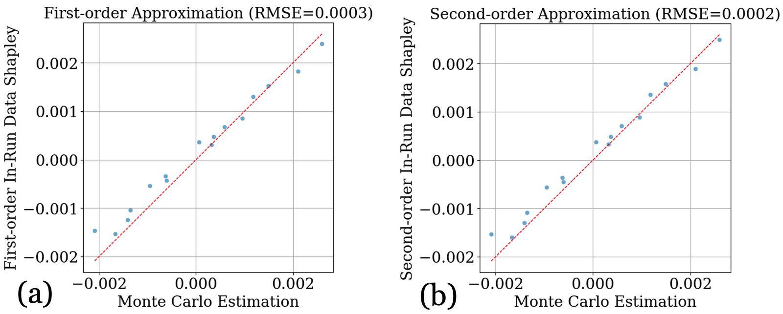
Figure 1: Comparison between the Monte Carlo-estimated In-Run Data Shapley and First/Second-order In-Run Data Shapley.
图 1:蒙特卡洛估计的 In-Run Data Shapley 与一/二阶 In-Run Data Shapley 的比较。
In this section, we directly assess the approximation accuracy of first- and second-order In-Run Data Shapley. In Appendix E.6, we further compare the performance of In-Run Data Shapley with existing (less scalable) data attribution techniques on standard benchmarks (e.g., mislabeled data detection) as an additional sanity check.
本节直接评估一、二阶 In-Run Data Shapley 的逼近精度。附录 E.6 进一步在标准基准(如错标检测)上与既有(可扩展性较差的)数据归因技术比较,作为额外健全性检查。
Given that computing the exact In-Run Data Shapley value is computationally prohibitive, we compare their performance against Monte Carlo estimates of the Shapley value using a large number of samples. The experiment is conducted on GPT2 model at the 3500th training iteration on Pile, where the batch size 16 and learning rate . We use 1000 permutations to approximate the groundtruth In-Run Shapley value. Figure 1 shows that with just first-order In-Run Data Shapley, the root mean squared error (RMSE) is only around 0.0003. In Appendix E.2.1, we provide additional results with different learning rates.
精确 In-Run Data Shapley 计算代价过高,故与用大量样本的蒙特卡洛 Shapley 估计比较。实验在 Pile 上 GPT2 训练的第 3500 步进行,批大小 16、学习率 ,用 1000 个置换逼近真实 In-Run Shapley。图 1 显示:仅一阶 In-Run Data Shapley,均方根误差(RMSE)就仅约 0.0003。附录 E.2.1 给出不同学习率的补充结果。
5.3 Case Study: Data Attribution on Pile Dataset
In this section, we present a case study to demonstrate the use cases of In-Run Data Shapley by pretraining on the well-known Pile dataset (Gao et al., 2020). We explore its application in data curation, examine data contribution across different training stages, and investigate relevant corpus detection. Due to computational resource constraints, most of our experiments focus on the GPT-2 and Pythia-410M models, but this is not a limitation of the algorithm itself. With adequate computational resources, our approach can easily be applied to larger-scale models.
本节以知名 Pile 数据集(Gao 等, 2020)上的预训练为例,展示 In-Run Data Shapley 的用例:数据策展、不同训练阶段的数据贡献,以及相关语料检测。受算力限制,多数实验聚焦 GPT-2 与 Pythia-410M,但这并非算法本身的限制;算力充足时方法可轻松用于更大规模模型。
5.3.1 Is Well-curated Dataset Actually Clean?
Carefully curated pretraining corpora still contain data points that can adversely affect the training process. Identifying and removing these data points can accelerate model convergence and enhance overall performance, thereby saving computational resources. In this experiment, we demonstrate the effectiveness of In-Run Data Shapley in assessing the data quality of a subset of the Pile dataset. We uniformly select a random subset of Pile with around 10B tokens and train a GPT2 model on this subset. We compute the data attribution results with Pile’s validation set. By filtering out all negatively valued corpora and retraining the model on the cleaned subset, we observe significant improvement in model convergence. For both first- and second-order In-Run Data Shapely, we can achieve around 25% fewer training iterations to reach a test loss of 3.75. Surprisingly, our analysis reveals that around 16% of the training corpora had negative second-order In-Run Data Shapley values. While some of the negatively valued corpora may be attributed to the significant domain shift compared to the validation corpora, we still find many low-quality corpora from Pile, a pretraining dataset that has undergone several layers of data curation (Gao et al., 2020). Examples of low-quality corpora identified can be found in Appendix E.3.
5.3.1 精心策展的数据集真的干净吗?
即便精心策展的预训练语料,仍含会不利影响训练的数据点。识别并移除它们可加速收敛、提升整体表现,从而节省算力。本实验展示 In-Run Data Shapley 评估 Pile 子集数据质量的效果。我们均匀随机抽取约 10B token 的 Pile 子集并训练 GPT2,用 Pile 验证集做归因。滤掉所有负值语料并在清洗子集上重训后,收敛显著改善:一、二阶 In-Run Data Shapley 都能以约少 25% 的训练迭代达到测试损失 3.75。出人意料,约 16% 训练语料的二阶 In-Run Data Shapley 为负。部分负值或因相对验证语料的显著领域偏移,但我们仍在已经过多层策展的 Pile(Gao 等, 2020)中发现大量低质语料。识别出的低质语料示例见附录 E.3。
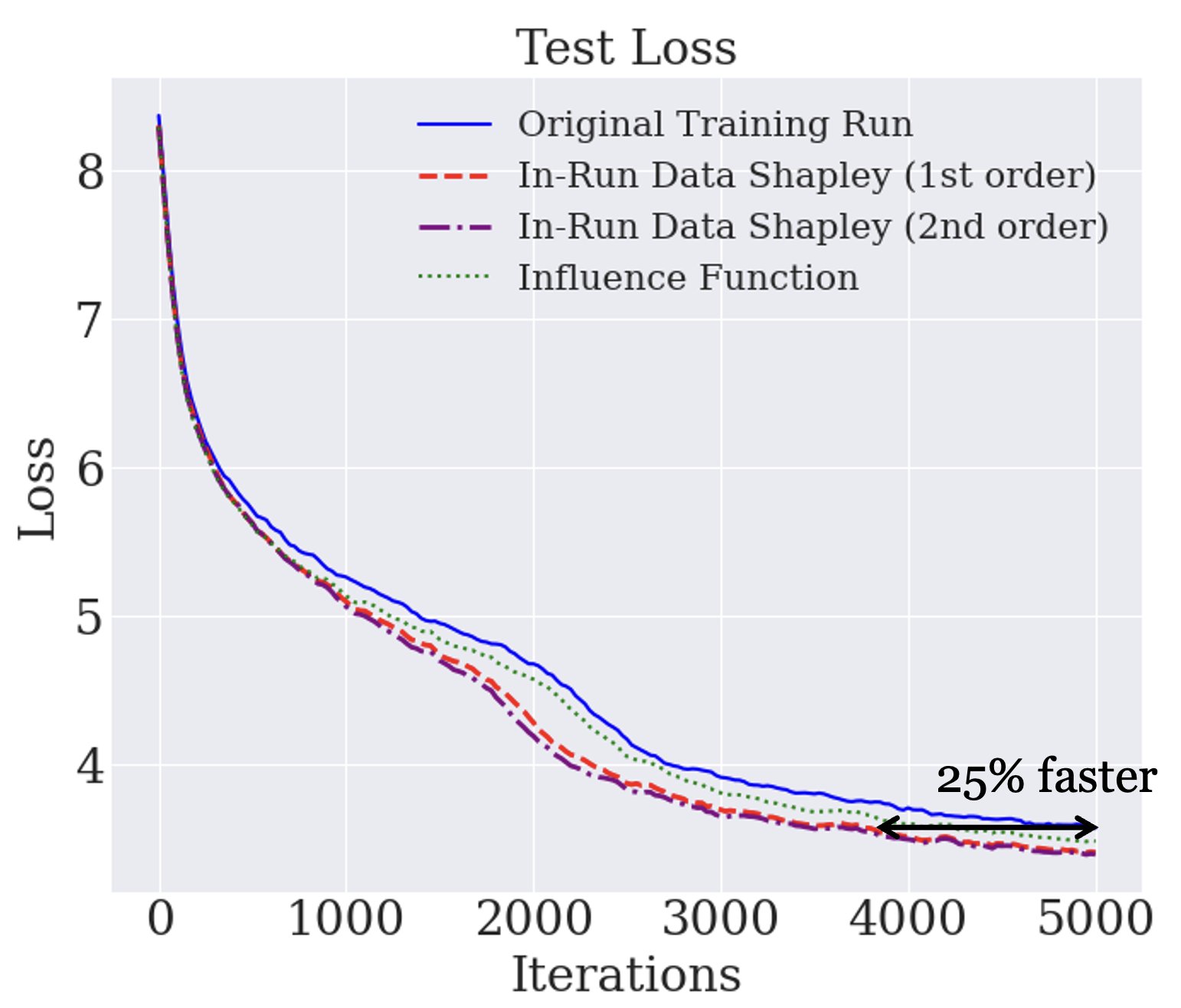
Figure 2: Test loss comparison between the original training run and the model trained on the cleaned subset according to different data attribution techniques.
图 2:原训练与按不同数据归因技术清洗子集后训练的测试损失比较。
Figure 2 shows a performance comparison between the original training run and the model trained on the cleaned subsets for GPT2, and additional results on Pythia-410M are available in Appendix E.3.1. We also compare with influence function (Koh & Liang, 2017), which approximates the change in the model’s loss on the test example when the training example is removed from the training set (i.e., the leave-one-out score). We omit TRAK (Park et al., 2023) and other techniques such as datamodel (Ilyas et al., 2022) as they are not scalable to our setting. As we can see, influence function can also filter out low-quality data that can accelerate training convergence. However, the performance is slightly worse than In-Run Data Shapley as the influence function only uses information from the final trained models, which can result in highly noisy value scores since the removal of one training data point might have a negligible effect on the final model performance. The results demonstrate that removing lower-quality data leads to a significantly faster drop in test loss compared to the original training run. This implies that there is still huge room for data curation for well-curated datasets such as Pile.
图 2 比较 GPT2 上原训练与清洗子集训练的表现;Pythia-410M 的补充结果见附录 E.3.1。我们也与影响函数(Koh & Liang, 2017)比较——它近似从训练集去掉某训练样本时测试损失的变化(即留一分数)。省略 TRAK(Park 等, 2023)与 datamodel(Ilyas 等, 2022)等,因其对本设定不可扩展。可见影响函数也能滤掉可加速收敛的低质数据,但略差于 In-Run Data Shapley:它只用最终已训模型的信息,去掉单点对最终表现影响可能微乎其微,价值分数因而噪声很大。结果表明去掉较低质量数据后,测试损失下降显著快于原训练,意味着即便如 Pile 这样已策展的数据集,数据策展仍有巨大空间。
| Similarity Category | In-Run Data Shapley (1st order) | In-Run Data Shapley (2nd order) | Influence Function | BM25 |
|---|---|---|---|---|
| Partial exactly the same | 1 | 1 | 1 | 1 |
| Paraphrase | 1 | 1 | 1 | 1 |
| Significant paraphrase | 32.3 | 32 | 39.3 | 1.6 |
| Similar topic | 145.6 | 141.6 | 292 | 20917.3 |
Table 2: Top: (left) An original training corpus from Wikipedia. (right) A synthetic corpus falls in the category of "Similar topic" to the Wikipedia corpus on the left (prompt in Appendix E.5). Bottom: the (average) value rank of the original corpus among all training corpora for validation corpora that are of varying similarity to the original corpus. The rank is out of 320k data points.
| 相似度类别 | In-Run Data Shapley(一阶) | In-Run Data Shapley(二阶) | 影响函数 | BM25 |
|---|---|---|---|---|
| 部分完全相同 | 1 | 1 | 1 | 1 |
| 改写 | 1 | 1 | 1 | 1 |
| 大幅改写 | 32.3 | 32 | 39.3 | 1.6 |
| 相似主题 | 145.6 | 141.6 | 292 | 20917.3 |
表 2:上:(左)来自 Wikipedia 的原始训练语料。(右)与左侧 Wikipedia 语料属「相似主题」的合成语料(提示见附录 E.5)。下:对与原始语料相似度不等的验证语料,原始语料在全部训练语料中的(平均)价值排名。排名基于约 32 万数据点。
Validation Corpus
In several applications, the matrix coefficients of the nonlinear valued function in are usually of low rank …
High-valued Corpus
The Lagrangian describes (axial-)vector meson interactions, see Appendix of Ref. [@Gallas]. After …
Low-valued Corpus
Coronavirus Testing in San Diego Countyn How San Diego Is Getting Ready for Self-Driving Cars …
Figure 3: Left: Domain value composition for a corpus of math text. Right: The math corpus we use as the validation data for attribution, and examples of high- and low-valued training corpus for it.
验证语料
在若干应用中,非线性赋值函数 的矩阵系数通常低秩……
高价值语料
Lagrangian 描述(轴)矢量介子相互作用,见文献 [@Gallas] 附录。在……
低价值语料
Coronavirus Testing in San Diego Countyn How San Diego Is Getting Ready for Self-Driving Cars ……
图 3:左:某数学文本语料的领域价值构成。右:用作归因验证的数学语料,以及对其高/低价值训练语料示例。
5.3.2 How Do Data Values Change during Training?
As In-Run Data Shapley tracks the cumulative data values across different training steps, we can assess the contribution of training points at various stages of training, providing a more fine-grained perspective on data attribution. We evaluate the data attribution results for a math-related validation data using second-order In-Run Data Shapley. In Figure 3, we present the value composition of training corpora by their domains over the first 10,000 training iterations, summing the values of all corpora from the same domain. We then calculate the percentage of the total value attributed to each domain, excluding domains with a total value . As illustrated in the figure, the corpora from ArXiv achieve a significantly higher value compared to other domain corpora, far exceeding its size proportion within the full Pile dataset. This is expected, as ArXiv papers predominantly cover fields like Math, Computer Science, and Physics, which contain extensive math-related content. Furthermore, the value composition changes rapidly at the beginning of training and stabilizes as training progresses. We hypothesize that this initial fluctuation is due to the presence of relevant paragraphs in corpora from other domains. The stable value proportion observed in later stages likely reflects the relative abundance of math content in each domain. Interestingly, we observe that Pile-CC domain, which contains general website crawls, initially shows positive contributions during the first few iterations. However, its value quickly drops to negative and eventually converges to zero. This implies that general corpora tend to have a large contribution in the beginning of training, as they help the model learn the basics of languages, such as grammar and common knowledge. However, as training progresses and the model focuses on more specialized topics, the relevance of general domains diminishes. An additional figure for the average domain values is in Appendix E.4.
5.3.2 训练过程中数据价值如何变化?
In-Run Data Shapley 跟踪不同训练步上的累计数据价值,因而可评估各阶段训练点的贡献,给出更细的归因视角。我们对某数学相关验证数据用二阶 In-Run Data Shapley 做归因。图 3 给出前 10,000 次迭代中训练语料按领域的价值构成:同领域语料价值求和,再算各领域占总价值的百分比(总价值 的领域排除)。如图所示,ArXiv 语料价值远高于其他领域,也远超其在完整 Pile 中的体量占比——这符合预期,因 ArXiv 论文多属数学、计算机与物理,含大量数学相关内容。此外,价值构成在训练初期变化很快,随后趋于稳定。我们猜测初期波动来自其他领域语料中夹杂的相关段落;后期稳定比例则更反映各领域数学内容的相对丰度。有趣的是,含通用网页抓取的 Pile-CC 在最初几次迭代呈正贡献,但很快降为负并最终收敛到零。这意味着 通用语料往往在训练初期贡献较大,帮助模型学习语法与常识等语言基础;随着训练推进、模型聚焦更专门主题,通用领域的相关性减弱。领域平均价值的补充图见附录 E.4。
5.3.3 Does Contribution Require Memorization?
In this experiment, we evaluate the robustness of different data attribution techniques in identifying relevant individual corpora that have been paraphrased. We start by selecting a data point from the training set and creating several paraphrased versions using GPT-4, with varying levels of paraphrasing (see Appendix E.5 for the prompt). These paraphrased versions form our validation set. We then calculate the average value rank of the original training data for each of its paraphrased versions. In addition to In-Run Data Shapley and influence function, we include the ranking result based on BM25 distance. BM25 (Robertson et al., 2009) featurizes examples by their word frequency statistics (i.e., TF-IDF) to rank the training instances. We use BM25 distance as an oracle for assessing the verbatim or lexical similarity between the validation data (query) and the training data, as opposed to semantic similarity.
5.3.3 贡献是否要求记忆?
本实验评估不同数据归因技术在识别「已被改写」的相关个体语料上的稳健性。我们从训练集选一点,用 GPT-4 生成不同程度的改写版本(提示见附录 E.5)作为验证集,再计算原始训练数据对其各改写版的平均价值排名。除 In-Run Data Shapley 与影响函数外,还加入基于 BM25 距离的排名。BM25(Robertson 等, 2009)用词频统计(即 TF-IDF)特征化样例以排序训练实例。我们用 BM25 距离作为评估验证数据(查询)与训练数据之间字面/词汇相似度——相对语义相似度——的 oracle。
As shown in Table 2, even for a validation data that is a complete rewrite (with a low BM25 distance) but covers relevant topics, the original training data still ranks very high according to both In-Run Data Shapley and influence function. Influence function ranks the original training data lower than In-Run Data Shapley, which may be attributed to the inherent noisy nature of the leave-one-out error estimation. The results of this experiment have important implications for the ongoing discussion about the copyright of generative AI. Specifically, the table presents a compelling example where the original Wikipedia training corpus related to a musician’s experience can significantly contribute to generating a story about a musician, even when the generated story shares no token-wise resemblance to the original training data. This finding supports that training data profoundly influences the capabilities of generative AI models and should be compensated accordingly (Deng & Ma, 2023; Wang et al., 2024b), even when the output does not closely resemble the original copyrighted material or when the model applies output filters to avoid generating verbatim replicates of the training data. This discovery expands the conventional focus on copyright violations, which typically addresses instances of near-verbatim replication, as seen in the dispute between New York Times and OpenAI, to also include cases where the generated content is significantly influenced by copyrighted material without directly replicating it.
如表 2,即便验证数据是完全改写(BM25 距离低)但主题相关,原始训练数据在 In-Run Data Shapley 与影响函数下仍排名很高。影响函数对原始训练数据的排名低于 In-Run Data Shapley,或因留一误差估计固有噪声。该结果对生成式 AI 版权讨论有重要含义。表中有一个有说服力的例子:与某音乐家经历相关的原始 Wikipedia 训练语料,可显著贡献于生成「关于音乐家的故事」,即便生成故事与原训练数据在 token 层面毫无相似。这支持:训练数据深刻影响生成式 AI 能力,应获相应补偿(Deng & Ma, 2023;Wang 等, 2024b)——即便输出并不酷似原版权材料,或模型用输出过滤避免逐字复现训练数据。该发现把版权侵权的传统焦点——多针对近乎逐字复制,如《纽约时报》与 OpenAI 之争——扩展到「生成内容受版权材料显著影响却未直接复制」的情形。
6 Conclusion and Limitations
In this work, we introduce In-Run Data Shapley, a novel data attribution technique that addresses the limitations of Retraining-based Data Shapley. Extensive experiments demonstrate the effectiveness of In-Run Data Shapley in various applications. Here, we discuss the potential limitations of this work.
本文提出 In-Run Data Shapley,一种应对基于重训的 Data Shapley 局限的新数据归因技术。大量实验展示了其在多种应用中的有效性。这里讨论潜在局限。
Availability of validation data before training. One potential limitation of In-Run Data Shapley is that it requires the validation data to be available before training, as the data attribution scores are computed during the training process. However, there are many scenarios where validation data is naturally available before training, such as when using publicly available benchmark datasets, participating in machine learning competitions, or adhering to regulatory requirements. For scenarios where validation data arrives after the model has been trained, a potential solution is to save checkpoints of intermediate models during training and approximate In-Run Data Shapley using these checkpoints, in the same spirit of TracIN-CP described in Pruthi et al. (2020). However, the choice of checkpoints can significantly impact performance, and it is unclear which checkpoints to pick.
训练前验证数据的可用性。 In-Run Data Shapley 的潜在局限之一是:归因分数在训练过程中计算,因而要求验证数据在训练前可用。不过许多场景下验证数据本来就在训练前可得,例如使用公开基准、参加机器学习竞赛,或满足监管要求。若验证数据在模型训完后才到达,一个可能办法是保存中间检查点,并仿照 Pruthi 等 (2020) 的 TracIN-CP,用这些检查点近似 In-Run Data Shapley。但检查点选择会显著影响表现,选哪些仍不清楚。
Extension to other optimization algorithms. Extending the "ghost" family techniques developed in this work to support Adam and similar optimizers remains an exciting direction for future research. We stress that extending the formulation of In-Run Data Shapley from SGD to Adam is feasible, but the actual challenge lies in computing it efficiently without instantiating each individual gradient vector, which cannot be solved by simple extensions described in Xia et al. (2024).
扩展到其他优化算法。 将本文「ghost」族技术扩展到 Adam 及类似优化器仍是有吸引力的未来方向。我们强调:把 In-Run Data Shapley 从 SGD 形式推广到 Adam 是可行的,真正挑战在于不实例化每个个体梯度向量而高效计算——这无法被 Xia 等 (2024) 所述的简单扩展解决。
Handling memory constraints. In scenarios where GPU memory constraints prevent large batch sizes, the "ghost" techniques can be extended by using gradient accumulation. This approach accommodates larger training batch sizes by dividing the batch into smaller sub-batches and accumulating gradients over multiple iterations. While this method may increase runtime due to additional backpropagation steps, it maintains the feasibility of the techniques under memory constraints. Improving computational efficiency for large batch sizes remains an important direction for future research.
处理显存约束。 当 GPU 显存限制大 batch 时,「ghost」技术可通过梯度累积扩展:把大批拆成更小的子批,在多次迭代上累积梯度。虽可能因额外反向增加运行时间,但在显存约束下仍保持可行性。提升大批量时的计算效率仍是重要未来方向。
Acknowledgment
This work is supported in part by the National Science Foundation under grants IIS-2312794, IIS-2313130, OAC-2239622, Amazon-Virginia Tech Initiative in Efficient and Robust Machine Learning, and the Commonwealth Cyber Initiative.
本工作部分得到美国国家科学基金会资助(IIS-2312794、IIS-2313130、OAC-2239622),以及 Amazon–Virginia Tech Initiative in Efficient and Robust Machine Learning 与 Commonwealth Cyber Initiative 的支持。
We thank Meng Ding, Chong Xiang, Chendi Wang for their helpful feedback on the preliminary version of this work.
感谢 Meng Ding、Chong Xiang、Chendi Wang 对本文初稿的有益反馈。
References
Ash et al. (2019) Jordan T Ash, Chicheng Zhang, Akshay Krishnamurthy, John Langford, and Alekh Agarwal. Deep batch active learning by diverse, uncertain gradient lower bounds. In International Conference on Learning Representations , 2019.
Bae et al. (2022) Juhan Bae, Nathan Ng, Alston Lo, Marzyeh Ghassemi, and Roger B Grosse. If influence functions are the answer, then what is the question? Advances in Neural Information Processing Systems , 35:17953–17967, 2022.
Basu et al. (2021) S Basu, P Pope, and S Feizi. Influence functions in deep learning are fragile. In International Conference on Learning Representations (ICLR) , 2021.
Biderman et al. (2023) Stella Biderman, Hailey Schoelkopf, Quentin Gregory Anthony, Herbie Bradley, Kyle O’Brien, Eric Hallahan, Mohammad Aflah Khan, Shivanshu Purohit, USVSN Sai Prashanth, Edward Raff, et al. Pythia: A suite for analyzing large language models across training and scaling. In International Conference on Machine Learning , pp. 2397–2430. PMLR, 2023.
Bu et al. (2022) Zhiqi Bu, Jialin Mao, and Shiyun Xu. Scalable and efficient training of large convolutional neural networks with differential privacy. Advances in Neural Information Processing Systems , 35:38305–38318, 2022.
Bu et al. (2023) Zhiqi Bu, Yu-Xiang Wang, Sheng Zha, and George Karypis. Differentially private optimization on large model at small cost. In International Conference on Machine Learning , pp. 3192–3218. PMLR, 2023.
Burgess & Chapman (2021) Mark Alexander Burgess and Archie C Chapman. Approximating the shapley value using stratified empirical bernstein sampling. In IJCAI , pp. 73–81, 2021.
Choe et al. (2024) Sang Keun Choe, Hwijeen Ahn, Juhan Bae, Kewen Zhao, Minsoo Kang, Youngseog Chung, Adithya Pratapa, Willie Neiswanger, Emma Strubell, Teruko Mitamura, et al. What is your data worth to gpt? llm-scale data valuation with influence functions. arXiv preprint arXiv:2405.13954 , 2024.
Cook & Weisberg (1980) R Dennis Cook and Sanford Weisberg. Characterizations of an empirical influence function for detecting influential cases in regression. Technometrics , 22(4):495–508, 1980.
Covert et al. (2024) Ian Covert, Chanwoo Kim, Su-In Lee, James Zou, and Tatsunori Hashimoto. Stochastic amortization: A unified approach to accelerate feature and data attribution. arXiv preprint arXiv:2401.15866 , 2024.
Deng & Ma (2023) Junwei Deng and Jiaqi Ma. Computational copyright: Towards a royalty model for ai music generation platforms. arXiv preprint arXiv:2312.06646 , 2023.
Dhaliwal & Shintre (2018) Jasjeet Dhaliwal and Saurabh Shintre. Gradient similarity: An explainable approach to detect adversarial attacks against deep learning. arXiv preprint arXiv:1806.10707 , 2018.
Feldman & Zhang (2020) Vitaly Feldman and Chiyuan Zhang. What neural networks memorize and why: Discovering the long tail via influence estimation. Advances in Neural Information Processing Systems , 33:2881–2891, 2020.
Fort & Ganguli (2019) Stanislav Fort and Surya Ganguli. Emergent properties of the local geometry of neural loss landscapes. arXiv preprint arXiv:1910.05929 , 2019.
Gao et al. (2020) Leo Gao, Stella Biderman, Sid Black, Laurence Golding, Travis Hoppe, Charles Foster, Jason Phang, Horace He, Anish Thite, Noa Nabeshima, et al. The pile: An 800gb dataset of diverse text for language modeling. arXiv preprint arXiv:2101.00027 , 2020.
Ghorbani & Zou (2019) Amirata Ghorbani and James Zou. Data shapley: Equitable valuation of data for machine learning. In International Conference on Machine Learning , pp. 2242–2251. PMLR, 2019.
Ghorbani et al. (2020) Amirata Ghorbani, Michael Kim, and James Zou. A distributional framework for data valuation. In International Conference on Machine Learning , pp. 3535–3544. PMLR, 2020.
Grosse et al. (2023) Roger Grosse, Juhan Bae, Cem Anil, Nelson Elhage, Alex Tamkin, Amirhossein Tajdini, Benoit Steiner, Dustin Li, Esin Durmus, Ethan Perez, et al. Studying large language model generalization with influence functions. arXiv preprint arXiv:2308.03296 , 2023.
Grynbaum & Mac (2023) Michael M Grynbaum and Ryan Mac. The times sues openai and microsoft. The New York Times , pp. B1–B1, 2023.
Heikkilä (2023) Melissa Heikkilä. This new tool could give artists an edge over ai. https://www.technologyreview.com/2023/10/24/1082247/this-new-tool-could-give-artists-an-edge-over-ai/ , 2023.
Henderson et al. (2023) Peter Henderson, Xuechen Li, Dan Jurafsky, Tatsunori Hashimoto, Mark A Lemley, and Percy Liang. Foundation models and fair use. arXiv preprint arXiv:2303.15715 , 2023.
Illés & Kerényi (2019) Ferenc Illés and Péter Kerényi. Estimation of the shapley value by ergodic sampling. arXiv preprint arXiv:1906.05224 , 2019.
Ilyas et al. (2022) Andrew Ilyas, Sung Min Park, Logan Engstrom, Guillaume Leclerc, and Aleksander Madry. Datamodels: Predicting predictions from training data. arXiv preprint arXiv:2202.00622 , 2022.
Jia et al. (2019a) Ruoxi Jia, David Dao, Boxin Wang, Frances Ann Hubis, Nezihe Merve Gurel, Bo Li, Ce Zhang, Costas J Spanos, and Dawn Song. Efficient task-specific data valuation for nearest neighbor algorithms. Proceedings of the VLDB Endowment , 2019a.
Jia et al. (2019b) Ruoxi Jia, David Dao, Boxin Wang, Frances Ann Hubis, Nick Hynes, Nezihe Merve Gürel, Bo Li, Ce Zhang, Dawn Song, and Costas J Spanos. Towards efficient data valuation based on the shapley value. In The 22nd International Conference on Artificial Intelligence and Statistics , pp. 1167–1176. PMLR, 2019b.
Koh & Liang (2017) Pang Wei Koh and Percy Liang. Understanding black-box predictions via influence functions. In International Conference on Machine Learning , pp. 1885–1894. PMLR, 2017.
Kong & Munoz Medina (2024) Weiwei Kong and Andres Munoz Medina. A unified fast gradient clipping framework for dp-sgd. Advances in Neural Information Processing Systems , 36, 2024.
Kwon & Zou (2022) Yongchan Kwon and James Zou. Beta shapley: a unified and noise-reduced data valuation framework for machine learning. In International Conference on Artificial Intelligence and Statistics , pp. 8780–8802. PMLR, 2022.
Kwon et al. (2021) Yongchan Kwon, Manuel A Rivas, and James Zou. Efficient computation and analysis of distributional shapley values. In International Conference on Artificial Intelligence and Statistics , pp. 793–801. PMLR, 2021.
Lee & Kifer (2021) Jaewoo Lee and Daniel Kifer. Scaling up differentially private deep learning with fast per-example gradient clipping. Proceedings on Privacy Enhancing Technologies , 2021.
Li & Yu (2023) Weida Li and Yaoliang Yu. Faster approximation of probabilistic and distributional values via least squares. In The Twelfth International Conference on Learning Representations , 2023.
Li & Yu (2024) Weida Li and Yaoliang Yu. Robust data valuation with weighted banzhaf values. Advances in Neural Information Processing Systems , 36, 2024.
Li et al. (2021) Xuechen Li, Florian Tramer, Percy Liang, and Tatsunori Hashimoto. Large language models can be strong differentially private learners. In International Conference on Learning Representations , 2021.
Lin et al. (2022) Jinkun Lin, Anqi Zhang, Mathias Lécuyer, Jinyang Li, Aurojit Panda, and Siddhartha Sen. Measuring the effect of training data on deep learning predictions via randomized experiments. In International Conference on Machine Learning , pp. 13468–13504. PMLR, 2022.
Mitchell et al. (2022) Rory Mitchell, Joshua Cooper, Eibe Frank, and Geoffrey Holmes. Sampling permutations for shapley value estimation. 2022.
Mulligan & Li (2024) Caitlin Mulligan and James Li. Generative ai’s end run around copyright. AI Snake Oil , 2024. URL https://www.aisnakeoil.com/p/generative-ais-end-run-around-copyright .
Nguyen et al. (2023) Elisa Nguyen, Minjoon Seo, and Seong Joon Oh. A bayesian approach to analysing training data attribution in deep learning. Advances in Neural Information Processing Systems , 36, 2023.
Okhrati & Lipani (2021) Ramin Okhrati and Aldo Lipani. A multilinear sampling algorithm to estimate shapley values. In 2020 25th International Conference on Pattern Recognition (ICPR) , pp. 7992–7999. IEEE, 2021.
Park et al. (2023) Sung Min Park, Kristian Georgiev, Andrew Ilyas, Guillaume Leclerc, and Aleksander Madry. Trak: attributing model behavior at scale. In Proceedings of the 40th International Conference on Machine Learning , pp. 27074–27113, 2023.
Pruthi et al. (2020) Garima Pruthi, Frederick Liu, Satyen Kale, and Mukund Sundararajan. Estimating training data influence by tracing gradient descent. Advances in Neural Information Processing Systems , 33:19920–19930, 2020.
Radford et al. (2019) Alec Radford, Jeff Wu, Rewon Child, David Luan, Dario Amodei, and Ilya Sutskever. Language models are unsupervised multitask learners. 2019.
Raffel et al. (2020) Colin Raffel, Noam Shazeer, Adam Roberts, Katherine Lee, Sharan Narang, Michael Matena, Yanqi Zhou, Wei Li, and Peter J Liu. Exploring the limits of transfer learning with a unified text-to-text transformer. Journal of machine learning research , 21(140):1–67, 2020.
Robertson et al. (2009) Stephen Robertson, Hugo Zaragoza, et al. The probabilistic relevance framework: Bm25 and beyond. Foundations and Trends® in Information Retrieval , 3(4):333–389, 2009.
Rochette et al. (2020) Gaspar Rochette, Andre Manoel, and Eric W Tramel. Efficient per-example gradient computations in convolutional neural networks. In Workshop on Theory and Practice of Differential Privacy (TPDP) , 2020.
Schioppa (2024) Andrea Schioppa. Gradient sketches for training data attribution and studying the loss landscape. arXiv preprint arXiv:2402.03994 , 2024.
Shapley (1953) Lloyd S Shapley. A value for n-person games. Contributions to the Theory of Games , 2(28):307–317, 1953.
Søgaard et al. (2021) Anders Søgaard et al. Revisiting methods for finding influential examples. arXiv preprint arXiv:2111.04683 , 2021.
Touvron et al. (2023) Hugo Touvron, Thibaut Lavril, Gautier Izacard, Xavier Martinet, Marie-Anne Lachaux, Timothée Lacroix, Baptiste Rozière, Naman Goyal, Eric Hambro, Faisal Azhar, et al. Llama: Open and efficient foundation language models. arXiv preprint arXiv:2302.13971 , 2023.
Wang & Jia (2023a) Jiachen T Wang and Ruoxi Jia. Data banzhaf: A robust data valuation framework for machine learning. In International Conference on Artificial Intelligence and Statistics , pp. 6388–6421. PMLR, 2023a.
Wang & Jia (2023b) Jiachen T Wang and Ruoxi Jia. A note on" towards efficient data valuation based on the shapley value”. arXiv preprint arXiv:2302.11431 , 2023b.
Wang & Jia (2023c) Jiachen T Wang and Ruoxi Jia. A note on" efficient task-specific data valuation for nearest neighbor algorithms". arXiv preprint arXiv:2304.04258 , 2023c.
Wang et al. (2023) Jiachen T Wang, Yuqing Zhu, Yu-Xiang Wang, Ruoxi Jia, and Prateek Mittal. Threshold knn-shapley: A linear-time and privacy-friendly approach to data valuation. arXiv preprint arXiv:2308.15709 , 2023.
Wang et al. (2024a) Jiachen T Wang, Zhun Deng, Hiroaki Chiba-Okabe, Boaz Barak, and Weijie J Su. An economic solution to copyright challenges of generative ai. Technical report, 2024a.
Wang et al. (2024b) Jiachen T Wang, Zhun Deng, Hiroaki Chiba-Okabe, Boaz Barak, Weijie J Su, et al. An economic solution to copyright challenges of generative ai. arXiv preprint arXiv:2404.13964 , 2024b.
Wang et al. (2024c) Jiachen T Wang, Prateek Mittal, and Ruoxi Jia. Efficient data shapley for weighted nearest neighbor algorithms. arXiv preprint arXiv:2401.11103 , 2024c.
Wang et al. (2024d) Jiachen T Wang, Tianji Yang, James Zou, Yongchan Kwon, and Ruoxi Jia. Rethinking data shapley for data selection tasks: Misleads and merits. arXiv preprint arXiv:2405.03875 , 2024d.
Wang et al. (2020) Tianhao Wang, Johannes Rausch, Ce Zhang, Ruoxi Jia, and Dawn Song. A principled approach to data valuation for federated learning. In Federated Learning , pp. 153–167. Springer, 2020.
Xia et al. (2024) Mengzhou Xia, Sadhika Malladi, Suchin Gururangan, Sanjeev Arora, and Danqi Chen. Less: Selecting influential data for targeted instruction tuning. In Forty-first International Conference on Machine Learning , 2024.
Yang et al. (2024) Ziao Yang, Han Yue, Jian Chen, and Hongfu Liu. On the inflation of knn-shapley value. arXiv preprint arXiv:2405.17489 , 2024.
Yeh et al. (2022) Chih-Kuan Yeh, Ankur Taly, Mukund Sundararajan, Frederick Liu, and Pradeep Ravikumar. First is better than last for training data influence. arXiv preprint arXiv:2202.11844 , 2022.
Yu et al. (2020) Tianhe Yu, Saurabh Kumar, Abhishek Gupta, Sergey Levine, Karol Hausman, and Chelsea Finn. Gradient surgery for multi-task learning. Advances in Neural Information Processing Systems , 33:5824–5836, 2020.
Appendix A Extended Related Works
A.1 Data Shapley Axioms
Data Shapley is one of the first principled approaches to data attribution being proposed Ghorbani & Zou (2019); Jia et al. (2019b). Data Shapley is based on the famous Shapley value (Shapley, 1953). In almost all of the literature, the Shapley value is being justified as the unique value notion satisfying the following four axioms:
Data Shapley 是最早被提出的有原则数据归因方法之一(Ghorbani & Zou, 2019;Jia 等, 2019b),基于著名的 Shapley 值(Shapley, 1953)。几乎所有文献中,Shapley 值都被论证为满足以下四条公理的唯一价值概念:
- Null player: if for all , then .
- Symmetry: if for all , then .
- Linearity: For utility functions and any , .
- Efficiency: for every .
- 空参与者: 若对所有 有 ,则 。
- 对称性: 若对所有 有 ,则 。
- 线性性: 对效用函数 与任意 ,。
- 效率: 对每个 ,。
In plain words, null player axiom means the Shapley value will assign zero score to data points with no contribution. Symmetry axiom requires equal scores assigned to equally impactful data points, ensuring fairness. Efficiency axiom requires the sum of contribution scores equal to the total utility, meaning the scores always represent a share of the total utility. Linearity axiom means the Shapley value supports additive decomposition across multiple utility functions, allowing for the calculation of contributions to the entire test set by summing the scores of individual test points.
通俗地说,空参与者公理要求对无贡献数据点赋零分;对称性要求同等影响力的点得同等分,保证公平;效率要求贡献分之和等于总效用,分数始终是总效用的份额;线性性意味着 Shapley 值支持跨多个效用函数的可加分解,从而可用各测试点分数之和得到整个测试集上的贡献。
A.2 Data Shapley and Friends
Since its introduction in 2019 (Ghorbani & Zou, 2019; Jia et al., 2019b), Data Shapley has rapidly gained popularity as a principled solution for data attribution. Due to the computationally expensive nature of retraining-based Data Shapley, various Monte Carlo-based approximation algorithms have been developed (Jia et al., 2019b; Illés & Kerényi, 2019; Okhrati & Lipani, 2021; Burgess & Chapman, 2021; Mitchell et al., 2022; Lin et al., 2022; Wang & Jia, 2023b; Li & Yu, 2023; Covert et al., 2024), these methods still necessitate extensive computational resources due to repeated model retraining, which is clearly impractical for modern-sized ML models. Many of its variants have been proposed. Kwon & Zou (2022) argues that the efficiency axiom is not necessary for many machine learning applications, and the framework of semivalue is derived by relaxing the efficiency axiom. Lin et al. (2022) provide an alternative justification for semivalue based on causal inference and randomized experiments. Based on the framework of semivalue, Kwon & Zou (2022) propose Beta Shapley, which is a collection of semivalues that enjoy certain mathematical convenience. Wang & Jia (2023a) propose Data Banzhaf, and show that the Banzhaf value, another famous solution concept from cooperative game theory, achieves more stable valuation results under stochastic learning algorithms. Li & Yu (2024) further improves the valuation stability by considering value notions outside the scope of semivalue.
自 2019 年提出以来(Ghorbani & Zou, 2019;Jia 等, 2019b),Data Shapley 迅速成为数据归因的原则性方案。因基于重训的计算昂贵,出现多种蒙特卡洛近似算法(Jia 等, 2019b;Illés & Kerényi, 2019;Okhrati & Lipani, 2021;Burgess & Chapman, 2021;Mitchell 等, 2022;Lin 等, 2022;Wang & Jia, 2023b;Li & Yu, 2023;Covert 等, 2024),但反复重训仍需大量算力,对现代规模模型显然不现实。亦有许多变体:Kwon & Zou (2022) 认为效率公理对许多机器学习应用并非必要,并放松该公理得到 半价值(semivalue) 框架;Lin 等 (2022) 从因果推断与随机实验给出半价值的另一论证;在此框架上 Kwon & Zou (2022) 提出具有某些数学便利的 Beta Shapley;Wang & Jia (2023a) 提出 Data Banzhaf,表明合作博弈论中另一著名解概念 Banzhaf 值在随机学习算法下估值更稳;Li & Yu (2024) 进一步考虑半价值范围之外的概念以提升估值稳定性。
The classic leave-one-out error is also a semivalue, where the influence function (Cook & Weisberg, 1980; Koh & Liang, 2017; Grosse et al., 2023) is generally considered as its approximation. A concurrent work (Choe et al., 2024) leverages a similar gradient decomposition technique as our paper to speed up influence function calculation. However, several works have pointed out the fragility of influence function for deep learning models (Basu et al., 2021; Søgaard et al., 2021; Bae et al., 2022), due to the strong assumptions of training convergence and strongly convexity of the loss function. Nguyen et al. (2023) takes a Bayesian view of data attribution and is able to evaluate the variance of LOO. Unlike Nguyen et al. (2023), our work explicitly incorporates specific training randomness (e.g., model initialization, batch ordering) into the utility function definition, providing attribution scores that reflect contributions to the exact training trajectory.
经典留一误差也是半价值,影响函数(Cook & Weisberg, 1980;Koh & Liang, 2017;Grosse 等, 2023)一般被视为其近似。同期工作(Choe 等, 2024)用与本文类似的梯度分解加速影响函数计算。但多篇工作指出影响函数对深度学习模型脆弱(Basu 等, 2021;Søgaard 等, 2021;Bae 等, 2022),因其依赖训练收敛与损失强凸等强假设。Nguyen 等 (2023) 从贝叶斯视角做数据归因并能评估 LOO 方差。与 Nguyen 等 (2023) 不同,我们把具体训练随机性(如初始化、批顺序)显式编入效用定义,使归因分数反映对精确训练轨迹的贡献。
Another line of works focuses on improving the computational efficiency of Data Shapley by considering K nearest neighbor (KNN) as the surrogate learning algorithm for the original, potentially complicated deep learning models (Jia et al., 2019a; Wang & Jia, 2023c; Wang et al., 2023; Wang et al., 2024c; Yang et al., 2024). Ghorbani et al. (2020); Kwon et al. (2021); Li & Yu (2023) consider Distributional Shapley, a generalization of Data Shapley to data distribution. In federated learning setting, Wang et al. (2020) proposes a similar idea of computing the Shapley value for each federated learning round.
另一路线用 K 近邻(KNN)作原复杂深度学习模型的代理学习算法,以提升 Data Shapley 计算效率(Jia 等, 2019a;Wang & Jia, 2023c;Wang 等, 2023;Wang 等, 2024c;Yang 等, 2024)。Ghorbani 等 (2020);Kwon 等 (2021);Li & Yu (2023) 考虑面向数据分布的 Distributional Shapley。在联邦学习设定下,Wang 等 (2020) 提出对每一联邦轮次计算 Shapley 值的类似想法。
Remark 3.
Randomized Monte Carlo estimators can be inefficient and may produce unstable valuation results, potentially violating fairness axioms of the Shapley value (e.g., the Symmetry axiom) due to inherent approximation errors. In contrast, In-Run Data Shapley does not rely on Monte Carlo estimators. Instead, it computes the exact Shapley value for an approximated utility function via Taylor expansion. This approach adheres to the fairness axioms while ensuring the reliability and consistency of the data valuation results.
注记 3。
随机蒙特卡洛估计器可能低效,并因固有逼近误差产生不稳估值,可能违反 Shapley 值公平公理(如对称性)。相反,In-Run Data Shapley 不依赖蒙特卡洛;它通过对逼近效用(Taylor 展开)计算精确 Shapley 值,既遵守公平公理,又保证数据估值结果的可靠与一致。
A.3 Comparison with TracIN (Pruthi et al., 2020)
The form of first-order In-Run Data Shapley from Section 4.1 coincides with the TracIN-Ideal in Pruthi et al. (2020). This provides a new understanding of TracIN-Ideal as an approximation to In-Run Data Shapley. Both works face the technical challenge of requiring per-sample gradient computations during a single training run. Pruthi et al. (2020) proposes TracIN-CP, which mitigates the computational burden by examining only a subset of intermediate checkpoints during training. At each checkpoint, the individual gradients for the entire training set are computed, rather than for a sampled batch, under the assumption that each training example is visited exactly once between checkpoints. A recent work (Xia et al., 2024) leverages TracIN-CP, an approximation algorithm for TracIN-Ideal, for instruction-following data selection. This approach, however, may deviate significantly from the original TracIN-Ideal, with the final valuation results heavily dependent on the selected checkpoints. Furthermore, Pruthi et al. (2020)’s implementation is limited to the parameters of the last linear layer due to memory constraints, potentially biasing the measurement of data contribution. For instance, Yeh et al. (2022) suggests that the last layer of a neural network might exhibit a strong "cancellation effect," where the data influence of different examples have large, contradictory magnitudes. Additionally, Schioppa (2024) demonstrates that selecting different layers can distort data attribution scores. In contrast, this work introduces the "ghost dot-product" technique to efficiently compute the first-order In-Run Data Shapley (i.e., TracIN-Ideal) directly and accurately, without additional approximations.
第 4.1 节一阶 In-Run Data Shapley 的形式与 Pruthi 等 (2020) 的 TracIN-Ideal 一致,从而把 TracIN-Ideal 理解为对 In-Run Data Shapley 的一种逼近。两工作都面临单次训练中需逐样本梯度的技术挑战。Pruthi 等 (2020) 提出 TracIN-CP:只检查训练中部分中间检查点以减轻负担;在每个检查点对整个训练集(而非采样批)算个体梯度,并假设检查点之间每个训练例恰好被访问一次。近期工作(Xia 等, 2024)用 TracIN-Ideal 的近似算法 TracIN-CP 做指令遵循数据选择,但可能显著偏离原 TracIN-Ideal,最终估值严重依赖所选检查点。此外,受显存限制,Pruthi 等 (2020) 的实现仅覆盖最后线性层参数,可能偏置贡献度量——例如 Yeh 等 (2022) 指出末层可能有强「抵消效应」,不同样例影响幅度大且方向矛盾;Schioppa (2024) 也表明选不同层会扭曲归因分数。相反,本文引入「ghost 点积」技术,直接、准确地高效计算一阶 In-Run Data Shapley(即 TracIN-Ideal),无需额外近似。
Appendix B Additional Discussion
In this section, we provide additional discussion about In-Run Data Shapley as well as its comparison with Retraining-based Data Shapley. Figure 4 gives a more detailed overview of our algorithm, and Figure 5 provides a visualized comparison between Retraining-based and In-Run Data Shapley.
本节补充讨论 In-Run Data Shapley,并与基于重训的 Data Shapley 比较。图 4 更细地概览算法,图 5 可视化二者对比。
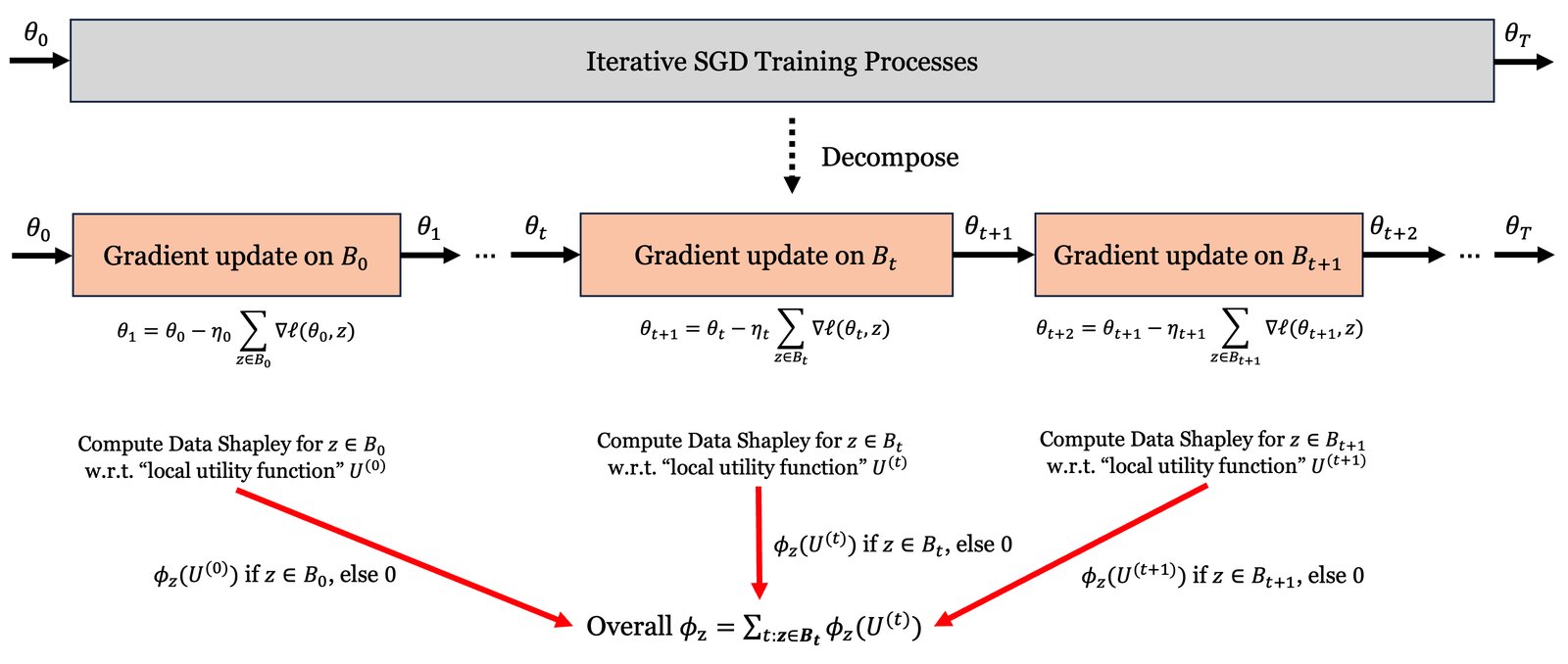
Figure 4: The core idea and algorithm overview of In-Run Data Shapley. Rather than evaluating data contribution across the entire training process (top), we decompose it into individual gradient update steps (bottom). For each iteration , we compute the Shapley value with respect to a "local utility function" that measures how the batch contributes to reducing validation loss. A data point’s final contribution score is the sum of its Shapley values across all iterations where it appears: . This decomposition approach maintains the Shapley value properties through the linearity axiom while making computation tractable.
图 4:In-Run Data Shapley 的核心想法与算法概览。与其评估整段训练上的数据贡献(上),我们将其分解为各梯度更新步(下)。对每次迭代 ,相对「局部效用」——衡量批 对降低验证损失的贡献——计算 Shapley 值 。数据点最终贡献分为其出现的所有迭代上 Shapley 值之和:。该分解通过线性性公理保持 Shapley 性质,同时使计算可处理。
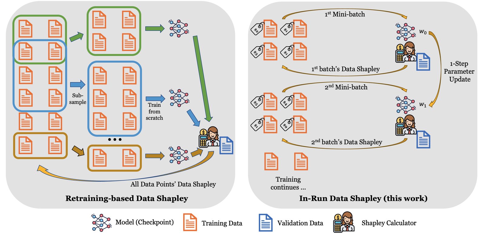
Figure 5: Comparison between Retraining-based and In-Run Data Shapley. Retraining-based Data Shapley requires training a model from scratch on all possible subsets of the full training set, which is computationally inefficient and raises concerns about interpretability and stability. In contrast, In-Run Data Shapley acts as a "contribution accountant", efficiently tracking and attributing data value scores to each training example across gradient update steps during a single training run.
图 5:基于重训与 In-Run Data Shapley 的比较。前者需在完整训练集的所有可能子集上从零训练,计算低效且有可解释性与稳定性之忧。后者像「贡献会计」,在单次训练中高效跟踪并为每个训练例跨梯度更新步归因价值分数。
B.1 When is In-Run Data Shapley Desirable for Data Attribution?
While Retraining-based Data Shapley has been widely adopted in the literature, it suffers from several critical issues that limit its practicality and effectiveness. In this section, we discuss these problems from four key aspects: computational efficiency, alignment with the purpose of data valuation, stability of the valuation results, and the choice of training hyperparameters.
尽管基于重训的 Data Shapley 在文献中被广泛采用,它仍有若干严重问题限制其实用性与有效性。本节从四方面讨论:计算效率、与数据估值目的的对齐、估值结果稳定性,以及训练超参选择。
(1) Computational burden. Retraining-based Data Shapley calculation is often computationally prohibitive, as it requires retraining the model on every possible subset of the original dataset, leading to a computational complexity that grows exponentially with the size of the dataset. Despite the development of various Monte Carlo-based approximation algorithms (Jia et al., 2019b; Illés & Kerényi, 2019; Okhrati & Lipani, 2021; Burgess & Chapman, 2021; Mitchell et al., 2022; Lin et al., 2022; Wang & Jia, 2023b; Li & Yu, 2023; Covert et al., 2024), these methods still necessitate extensive computational resources due to repeated model retraining, which is clearly impractical for modern-sized ML models. Another line of work attempts to use efficient proxy learning algorithms, such as -nearest neighbors (KNN) (Jia et al., 2019a; Wang & Jia, 2023c; Wang et al., 2023; Wang et al., 2024c; Yang et al., 2024), to accelerate Data Shapley computation. However, it remains unclear how closely these cheaper proxy models approximate the original learning algorithm, and it is also uncertain how to interpret the derived Data Shapley scores in this context.
(1)计算负担。 基于重训的 Data Shapley 往往计算上不可行:需在原数据集每个可能子集上重训,复杂度随数据规模指数增长。尽管有多种蒙特卡洛近似(Jia 等, 2019b;Illés & Kerényi, 2019;Okhrati & Lipani, 2021;Burgess & Chapman, 2021;Mitchell 等, 2022;Lin 等, 2022;Wang & Jia, 2023b;Li & Yu, 2023;Covert 等, 2024),反复重训仍需大量算力,对现代规模模型不现实。另一路线用 近邻(KNN)等高效代理学习算法加速(Jia 等, 2019a;Wang & Jia, 2023c;Wang 等, 2023;Wang 等, 2024c;Yang 等, 2024),但这些更便宜的代理与原学习算法有多接近仍不清楚,所得 Data Shapley 分数该如何解释也不确定。
(2) Retraining-based Data Shapley is unable to assess data contribution to a specific model. Crucially, Retraining-based Data Shapley is not designed to value data contribution towards a specific model. It attempts to quantify the average contribution of each training data point to models trained on different subsets of the data, rather than its contribution to the specific model trained on the full dataset. While one might interpret the former as an approximation of the latter, these two quantities can be quite different in practice, especially when the learning algorithm is randomized and sensitive to factors like random initialization and the order of the data points during training. More importantly, in most real-life scenarios, the primary interest lies in understanding the contribution of each data point to the specific model being trained and deployed.
(2)基于重训的 Data Shapley 无法评估对特定模型的数据贡献。 关键是:它并非为对某个具体模型估值数据贡献而设计。它试图量化各训练点对「在不同子集上训出的模型」的平均贡献,而非对「在全数据上训出的那个具体模型」的贡献。虽可将前者视为后者近似,实践中二者可相差甚远——尤其当学习算法随机、对初始化与数据顺序敏感时。更重要的是,多数真实场景真正关心的,正是正在训练并部署的那一个模型上各点的贡献。
(3) Retraining-based Data Shapley produces unstable valuation results for stochastic training algorithms. Furthermore, when the training algorithm involves randomness, such as in the case of SGD with random mini-batch selection, the corresponding utility function becomes randomized. Prior work (Wang & Jia, 2023a) suggests that this randomness can introduce substantial noise into the estimated Shapley values, rendering them unreliable and unstable. This instability poses significant challenges for interpreting and using the resulting data valuations, as the scores may vary considerably across different runs of the algorithm, even on the same dataset. Consequently, this limits the practical applicability of Retraining-based Data Shapley when working with stochastic training algorithms, which are prevalent in modern machine learning. We note that similar vulnerabilities to learning stochasticity have been observed for LOO-based data influence scores (e.g., influence function (Koh & Liang, 2017)) in several works (Basu et al., 2021; Søgaard et al., 2021; Nguyen et al., 2023).
(3)对随机训练算法,基于重训的 Data Shapley 估值不稳。 当训练含随机性(如带随机小批选择的 SGD)时,对应效用函数本身随机。先前工作(Wang & Jia, 2023a)指出,这种随机性会给估计的 Shapley 值引入大量噪声,使其不可靠、不稳定。分数在同数据集上不同运行间可大幅波动,给解释与使用带来挑战,从而限制其在现代机器学习常见随机训练算法下的实用性。我们注意到,若干工作(Basu 等, 2021;Søgaard 等, 2021;Nguyen 等, 2023)对基于 LOO 的数据影响分数(如影响函数(Koh & Liang, 2017))也观察到对学习随机性的类似脆弱。
(4) Training hyperparameter choices in Retraining-based Data Shapley are unclear. In machine learning, training hyperparameters (e.g., learning rate and batch size) typically need to be adjusted based on the size of the training dataset. This creates a fundamental ambiguity when computing Data Shapley values: when evaluating the utility for different data subsets , should we use the same hyperparameters as those optimized for the full dataset, or should we adjust them based on the subset size? This choice can significantly impact the calculated values.
(4)基于重训的 Data Shapley 中训练超参选择不明。 机器学习中,学习率与批大小等超参通常需随训练集规模调整。这在计算 Data Shapley 时造成根本含糊:对不同子集 评估效用 时,该用为全数据优化的同一超参,还是按子集规模调整?该选择会显著影响算出的价值。
In-Run Data Shapley addresses all these issues, making it more desirable for specific scenarios. Firstly, it is computationally efficient as it computes data values during the training run, avoiding the need for multiple retraining iterations. This makes it feasible for modern large-scale ML models. Secondly, it aligns better with the purpose of data valuation by assessing the contribution of each data point to the specific model being trained, providing more relevant insights for real-world applications. Lastly, In-Run Data Shapley offers deterministic valuation results even with stochastic training algorithms, as it incorporates the specific sequence and randomness of the training process into the utility function. Therefore, for scenarios where computational efficiency, model-specific contributions, and result stability are critical, In-Run Data Shapley is a more suitable choice.
In-Run Data Shapley 应对上述所有问题,在特定场景下更可取。首先,它在训练过程中算数据价值,无需多次重训,计算高效,对现代大规模模型可行。其次,它评估各点对正在训练的具体模型的贡献,更对齐数据估值目的,对现实应用更相关。最后,即便训练算法随机,它把具体序列与随机性编入效用,仍给出确定性估值。因此,当计算效率、模型特定贡献与结果稳定性关键时,In-Run Data Shapley 更合适。
Remark 4(In-run Data Shapley is a model-specific data attribution technique.).
In the original Data Shapley literature, typically defines utility as the final performance (e.g., accuracy, loss) of a model trained on a data subset . However, things become more complicated in the context of deep learning. A specific deep learning training run is an iterative process. Defining utility for a particular run makes it a sequence function rather than the pure set function required by the standard Shapley value framework. Extending Shapley axioms to sequence functions is not straightforward. Previous works often define as "expected model utility across all possible training runs" to circumvent this conceptual issue. In this work, we initiate the study of model-specific data attribution, which is crucial for applications like model diagnosis and behavior interpretation where we focus on a specific training run rather than expected utility across all possible runs.
注记 4(In-Run Data Shapley 是模型特定的数据归因技术。)。
在原始 Data Shapley 文献中, 通常把效用定义为在子集 上训练所得模型的最终表现(如准确率、损失)。但在深度学习语境下事情更复杂:一次具体深度学习训练是迭代过程*。为某次运行定义 使其成为序列函数,而非标准 Shapley 框架所需的纯集合函数;把公理扩到序列函数并不直接。先前工作常把 定义为「所有可能训练运行上的期望模型效用」以绕开该概念问题。本文开启对模型特定数据归因的研究——这对模型诊断与行为解释等应用至关重要,因为关注的是某次具体训练而非所有可能运行上的期望效用。*
Data attribution should consider specific application scenario. From a broader perspective, the "optimal data attribution" notion heavily depends on the intended application. In the literature, data attribution techniques are being used for various purposes such as data quality assessment, data valuation, and interpreting model predictions. For data quality assessment, we require "algorithm-level data attribution" that measures a data point’s general influence on the learning algorithm, independent of specific training random seeds. On the other hand, when interpreting model decisions, we need model-specific data attribution focused on the particular checkpoint we train. Systematically mapping which data attribution approaches best suit specific application scenarios remains an important direction for future research.
数据归因应考虑具体应用场景。更广地说,「最优数据归因」概念高度依赖预期应用。文献中数据归因被用于数据质量评估、数据估值与解释模型预测等。对数据质量评估,需要「算法级数据归因」,度量点对学习算法的一般影响,独立于具体训练随机种子;而解释模型决策时,需要聚焦所训具体检查点的模型特定归因。系统梳理何种归因方法最适合何种应用场景,仍是重要未来方向。
B.2 When is Retraining-based Data Shapley Desirable for Data Attribution?
Retraining-based Data Shapley is still desirable in several scenarios. Firstly, it is more general and applicable to all learning algorithms, whereas In-Run Data Shapley is only applicable to iterative training algorithms. Secondly, retraining-based Shapley is useful when the goal is to understand the contribution of data points to the general learning process rather than to a specific model. Thirdly, because Retraining-based Data Shapley does not require modifying the internal code of the training algorithm, its estimation algorithm, typically Monte Carlo-based, is straightforward and clean to implement.
基于重训的 Data Shapley 在若干场景仍可取。首先,它更通用,适用于所有学习算法,而 In-Run Data Shapley 仅适用于迭代训练算法。其次,当目标是理解数据点对一般学习过程——而非某个具体模型——的贡献时,基于重训的 Shapley 有用。第三,它无需修改训练算法内部代码,其估计算法(通常基于蒙特卡洛)实现直接、干净。
B.3 Potential Extensions of In-Run Data Shapley to Other Domains
While this work focuses on data attribution for SGD-trained machine learning models, we believe the core idea of In-Run Data Shapley—decomposing contribution analysis into per-iteration assessments—can potentially be extended to other contexts and applications. Here, we discuss some directions.
本文聚焦 SGD 训练的机器学习模型的数据归因,但我们相信 In-Run Data Shapley 的核心想法——把贡献分析分解为逐迭代评估——有望扩展到其他语境与应用。这里讨论若干方向。
Data attribution for iterative learning algorithms that do not use gradient descent. Our framework could potentially extend to iterative learning algorithms that don’t use gradient descent, such as k-means clustering or decision tree learning. Though these algorithms update models differently, they still proceed iteratively (e.g., k-means alternates between assignment and update steps; decision trees are built through recursive partitioning). For such algorithms, we could analyze how each data point influences these discrete update steps and aggregate these influences across iterations, similar to our approach with gradient-based training.
对不用梯度下降的迭代学习算法做数据归因。 框架或可扩展到 k-means、决策树学习等不用梯度下降的迭代算法。虽更新方式不同,它们仍迭代进行(如 k-means 在分配与更新间交替;决策树经递归划分构建)。对这类算法,可分析各数据点如何影响这些离散更新步,并像梯度训练一样跨迭代聚合影响。
Hyperparameter importance. The framework could potentially be adapted to evaluate hyperparameter contributions during training. One possibility is to set a "baseline" hyperparameter value and assess how choosing a different value impacts each training iteration compared to this baseline. For instance, when evaluating learning rate choices, we could measure how using a specific learning rate value affects model updates compared to using a baseline learning rate. For differentiable hyperparameters, we could leverage Taylor expansion to approximate this difference; for non-differentiable ones, zero-order methods could potentially be used. By accumulating these contributions across training iterations, we could understand hyperparameter impact without requiring multiple complete training runs. At a high level, this view unifies our treatment of training data and hyperparameters - both can be seen as choices that influence each training iteration, where we aim to quantify their impact against baseline scenarios. While technical challenges remain in adapting our method, this direction presents an interesting opportunity for future research.
超参重要性。 框架或可改编以评估训练中超参的贡献。一种可能是设「基线」超参值,评估相对基线换用另一值对每轮训练的影响。例如评估学习率选择时,可度量用某学习率相对基线学习率如何影响模型更新。对可微超参,可用 Taylor 展开逼近该差;对不可微者,或可用零阶方法。跨迭代累加这些贡献,便有望在无需多次完整训练的情况下理解超参影响。宏观上,这把训练数据与超参统一为影响每轮训练的选择,目标是相对基线量化其影响。虽改编方法仍有技术挑战,该方向是有趣的未来机会。
Feature attribution (e.g., context-attribution for language models). Another possible extension we envision is feature attribution for machine learning models. Feature attribution aims at understanding how each part of the input (like individual words in a sentence or pixels in an image) influences a model’s final prediction. When a model makes a prediction, the input features are processed through multiple layers, with each layer transforming the information before passing it to the next layer. Feature attribution aims to track how this information flows and transforms through the network to determine each input feature’s contribution to the final output. We envision a unified theoretical framework connecting training data attribution and feature attribution, drawing parallels between how information flows during training (through gradient updates) and during prediction (through layer operations). This could lead to more efficient methods for explaining model behavior, particularly for complex architectures like transformers.
特征归因(如语言模型的上下文归因)。 另一可能扩展是机器学习模型的特征归因:理解输入各部分(句子中的词、图像中的像素)如何影响最终预测。模型预测时,输入特征经多层处理,每层变换信息再传给下一层;特征归因旨在跟踪信息如何在网络中流动与变换,以确定各输入特征对最终输出的贡献。我们设想一个连接训练数据归因与特征归因的统一理论框架,类比训练中信息如何经梯度更新流动,与预测中如何经层运算流动。这或能带来更高效的模型行为解释方法,尤其对 transformer 等复杂架构。
Appendix C Missing Proofs
Theorem 5(Restate of Theorem 3).
In-Run Data Shapley considering the first-order approximation has closed-form
定理 5(定理 3 的重述)。
考虑一阶逼近的 In-Run Data Shapley 具有闭式
where
其中
Proof.
For notation simplicity, let . Given the utility function
证明。
为记号简洁,令 。给定效用函数
the marginal contribution of for any is
对任意 , 的边际贡献为
Plugging in the expression to the Shapley value’s definition immediately gives the result. ∎
将该表达式代入 Shapley 值定义即得结果。∎
Theorem 6(Restate of Theorem 4).
In-Run Data Shapley considering the second-order approximation has closed-form
定理 6(定理 4 的重述)。
考虑二阶逼近的 In-Run Data Shapley 具有闭式
where
其中
$$\displaystyle\phi_{z}\left(U^{(t)}{(1)}\right)+\frac{1}{2}\phi{z}\left(U^{(t)}{(2)}\right)=\underbrace{-\eta{t}\nabla\ell(w_{t},z^{(\mathrm{val})})\cdot\nabla\ell(w_{t},z)}{\text{\hbox to9.41pt{\vbox to9.41pt{\pgfpicture\makeatletter\hbox{\hskip 4.70488pt\lower-4.70488pt\hbox to0.0pt{\lxSVG@begingroup@{scopebegin=1} \lxSVG@begingroup@{stroke=#000000} \lxSVG@begingroup@{fill=#000000} \lxSVG@setlinewidth{\the\pgflinewidth}\lxSVG@begingroup@{stroke-width=0.4pt} \lx@inpgf@ignorespaces\nullfont\hbox to0.0pt{\lxSVG@begingroup@{scopebegin=1} {
{{}}\lx@inpgf@ignorespaces\hbox{\hbox{{\lxSVG@begingroup@{scopebegin=1} {{}{{{}}}{{}}{}{}{\lx@inpgf@ignorespaces}{\lx@inpgf@ignorespaces}{}{}{}{}{}{{}\lxSVG@stroke\lxSVG@drawpath@unclipped{M 6.23 0 C 6.23 3.44 3.44 6.23 0 6.23 C -3.44 6.23 -6.23 3.44 -6.23 0 C -6.23 -3.44 -3.44 -6.23 0 -6.23 C 3.44 -6.23 6.23 -3.44 6.23 0 Z M 0 0}{fill:none} \lx@inpgf@ignorespaces
}{{{{\lx@inpgf@ignorespaces}}\lxSVG@begingroup@{scopebegin=1} \lxSVG@transformcm{1.0}{0.0}{0.0}{1.0}{-2.11113pt}{-2.25555pt}\lxSVG@begingroup@{transform=matrix(1.0 0.0 0.0 1.0 -2.92 -3.12)} \pgfsys@hbox{63}\lxSVG@closescope }}}
\lxSVG@closescope }}}
}
\lxSVG@closescope {{{}}}{\lx@inpgf@ignorespaces}{\lx@inpgf@ignorespaces}\hss}\lxSVG@discardpath\lxSVG@closescope \hss}}\lxSVG@closescope\endpgfpicture}} influence of }z\text{ on the loss of }z^{(\mathrm{val})}}+\underbrace{\frac{\eta{t}^{2}}{2}\nabla\ell(w{t},z)^{\intercal}\textbf{H}^{(z^{(\mathrm{val})})}{t}\left(\sum{z{j}\in\mathcal{B}{t}}\nabla\ell(w{t},z_{j})\right)}_{\text{\hbox to9.41pt{\vbox to9.41pt{\pgfpicture\makeatletter\hbox{\hskip 4.70488pt\lower-4.70488pt\hbox to0.0pt{\lxSVG@begingroup@{_scopebegin=1} \lxSVG@begingroup@{stroke=#000000} \lxSVG@begingroup@{fill=#000000} \lxSVG@setlinewidth{\the\pgflinewidth}\lxSVG@begingroup@{stroke-width=0.4pt} \lx@inpgf@ignorespaces\nullfont\hbox to0.0pt{\lxSVG@begingroup@{_scopebegin=1} {
{{}}\lx@inpgf@ignorespaces\hbox{\hbox{{\lxSVG@begingroup@{_scopebegin=1} {{}{{{}}}{{}}{}{}{\lx@inpgf@ignorespaces}{\lx@inpgf@ignorespaces}{}{}{}{}{}{{}\lxSVG@stroke\lxSVG@drawpath@unclipped{M 6.23 0 C 6.23 3.44 3.44 6.23 0 6.23 C -3.44 6.23 -6.23 3.44 -6.23 0 C -6.23 -3.44 -3.44 -6.23 0 -6.23 C 3.44 -6.23 6.23 -3.44 6.23 0 Z M 0 0}{fill:none} \lx@inpgf@ignorespaces
}{{{{\lx@inpgf@ignorespaces}}\lxSVG@begingroup@{_scopebegin=1} \lxSVG@transformcm{1.0}{0.0}{0.0}{1.0}{-2.11113pt}{-2.25555pt}\lxSVG@begingroup@{transform=matrix(1.0 0.0 0.0 1.0 -2.92 -3.12)} \pgfsys@hbox{63}\lxSVG@closescope }}}
\lxSVG@closescope }}}
}
\lxSVG@closescope {{{}}}{\lx@inpgf@ignorespaces}{\lx@inpgf@ignorespaces}\hss}\lxSVG@discardpath\lxSVG@closescope \hss}}\lxSVG@closescope\endpgfpicture}} interaction between }z\text{ and other training points}} \tag{7}$$
for any .
对任意 。
Proof.
We show that
证明。
我们证明
For notation simplicity, let , and . Furthermore, let the batch size in -th iteration. For any , the marginal contribution of is
为记号简洁,令 ,;再令 为第 轮批大小。对任意 , 的边际贡献为
Plug the above expression into the Shapley value’s formula, we have
将上式代入 Shapley 值公式,得
∎
Appendix D Technical Details
Notation review. Consider a linear layer , where is the weight matrix, is the mini-batch input, and is the output (i.e., the pre-activation tensor). For non-sequential data, . For sequential data with sequence length , . Let denote the current model’s individual loss on . For notation convenience, we denote .
记号回顾。 考虑线性层 ,权矩阵 ,小批输入 ,输出(预激活)。对非序列数据,;对序列长度 的序列数据,。记 为当前模型在 上的个体损失。为方便,记 。
D.1 Ghost Dot-Product
By applying the chain rule, we can express the gradient of an individual loss with respect to W as
由链式法则,个体损失 对 W 的梯度可写为
where is the aggregated loss. Note that the individual’s output gradient is readily available during the backpropagation pass.
其中 为聚合损失。注意个体输出梯度 在反向传播中已经可得。
Suppose we are interested in computing the gradient dot-product between two data points in the same batch in the backpropagation. We first discuss the case for non-sequential data and then extend it to sequential data.
假设我们关心同批两点 在反向中的梯度点积 。先讨论非序列数据,再扩到序列数据。
Non-sequential data. For non-sequential data, we have each and . By (8), we have
非序列数据。 对非序列数据,有 、。由 (8) 得
Hence, we can compute the dot-product between and without actually instantiating the gradient vector or . We can take the dot products between and , and then multiply the results together. Moreover, all of the materials that are required for computation are all already available in one backpropagation. Hence, with a single backpropagation, we can efficiently compute the gradient dot-product between every pair of data points within the batch.
于是无需真正实例化梯度向量 或 ,即可算二者点积:先分别对 与 取点积再相乘。而且计算所需的 在一次反向中皆已可得。故单次反向即可高效算出批内每一对数据点的梯度点积。
Sequential data. For sequential data, we have each and . By (8), we have
序列数据。 对序列数据,有 、。由 (8) 得
Hence, comparing with directly computing per-sample gradients, if , it is more memory-efficient to first multiply the matrices of and , then take the inner product between the two matrices. If , then we can first take the outer products and , then take their inner product. In either case, we only need a single backpropagation to compute the gradient dot product between every pair of data points within the batch, similar to the case of non-sequential data.
因此,相对直接算逐样本梯度:若 ,更省显存的做法是先乘 与 ,再对两个 矩阵取内积;若 ,则可先取外积 与 ,再取其内积。无论哪种情形,都只需单次反向即可算批内每一对的梯度点积,与非序列情形类似。
Remark 5(Applications of "Ghost" Technique Beyond Data Attribution).
The techniques developed in this work for efficiently computing gradient dot products may be of independent interest, as this operation arises in various machine learning algorithms and applications beyond data attribution. For instance, the "ghost dot-product" technique can be used in calculating the cosine similarity between individual gradients (together with the "ghost clipping" technique), which is frequently being employed to analyze training dynamics (Fort & Ganguli, 2019) and detect adversarial attacks (Dhaliwal & Shintre, 2018). Additionally, gradient similarity is used in active learning to select the most informative data points for labeling (Ash et al., 2019) and in multitask learning to balance the contributions of different tasks (Yu et al., 2020).
注记 5(「Ghost」技术在数据归因之外的应用)。
本文为高效计算梯度点积发展的技术或有独立兴趣,因该运算出现在数据归因之外的多种机器学习算法与应用中。例如,「ghost 点积」可与「ghost clipping」一道用于计算个体梯度间的余弦相似度,常被用来分析训练动态(Fort & Ganguli, 2019)与检测对抗攻击(Dhaliwal & Shintre, 2018)。此外,梯度相似度用于主动学习以选择最有信息量的标注点(Ash 等, 2019),以及多任务学习中平衡不同任务贡献(Yu 等, 2020)。
D.2 Ghost Gradient-Hessian-Gradient Product
We denote as the number of layers in a neural network, and we denote , as the weight parameters of each layer. We denote as the Hessian matrix of on layer . Suppose we are interested in computing the gradient dot product .
记神经网络层数为 ,各层权重为 ,。记 为 在层 上的 Hessian。假设我们关心梯度点积 。
We first look at the Hessian-vector product.
我们先看 Hessian–向量积。
where we denote and .
其中记 、。
We run the second backpropagation on the gradient dot product . Note that here are constant vectors. For , we have the similar decomposition
我们对梯度点积 做第二次反向。注意此处 为常向量。对 ,有类似分解
For , the derivative is more complicated as the also depends on the output from deeper layers. When , we still have
对 ,因 还依赖更深一层的输出,导数更复杂。当 时,仍有
When , we have
当 时,有
Overall,
总体地,
$$\displaystyle\frac{\partial\textbf{d}{j}}{\partial\textbf{W}{i}} \ \displaystyle=\frac{\partial}{\partial\textbf{W}{i}}(\textbf{b}^{(z^{(\mathrm{val})})}{j}\textbf{b}^{(2)}{j}) \ \displaystyle=\begin{cases}\frac{\partial}{\partial\textbf{s}^{(z^{(\mathrm{val})})}{i}}\left(\textbf{b}^{(z^{(\mathrm{val})})}{j}\textbf{b}^{(2)}{j}\right)\otimes\textbf{a}^{(z^{(\mathrm{val})})}{i}&j\geq i\
\frac{\partial}{\partial\textbf{s}^{(z^{(\mathrm{val})})}{i}}\left(\textbf{b}^{(z^{(\mathrm{val})})}{j}\textbf{b}^{(2)}{j}\right)\otimes\textbf{a}^{(z^{(\mathrm{val})})}{i}+\textbf{b}^{(z^{(\mathrm{val})})}{i}\otimes\left(\frac{\partial\textbf{a}^{(z^{(\mathrm{val})})}{i}}{\partial\textbf{s}^{(z^{(\mathrm{val})})}{j}}\textbf{b}^{(2)}_{j}\right)&j<i\
\end{cases}$$
Hence, we have
因此有
$$\displaystyle\nabla\ell^{(1)}\textbf{H}^{(z^{(\mathrm{val})})}\nabla\ell^{(2)} \ \displaystyle=\sum_{i,j=1}^{L,L}(\textbf{a}^{(1)}{i}\otimes\textbf{b}^{(1)}{i})\left[\textbf{c}{j}\frac{\partial\textbf{d}{j}}{\partial\textbf{W}{i}}+\textbf{d}{j}\frac{\partial\textbf{c}{j}}{\partial\textbf{W}{i}}\right] \ \displaystyle=\underbrace{\sum_{i,j=1}^{L,L}(\textbf{a}^{(1)}{i}\otimes\textbf{b}^{(1)}{i})\left(\frac{\partial}{\partial\textbf{s}^{(z^{(\mathrm{val})})}{i}}\left(\textbf{c}{j}\textbf{d}{j}\right)\otimes\textbf{a}^{(z^{(\mathrm{val})})}{i}\right)}{\hbox to9.22pt{\vbox to9.22pt{\pgfpicture\makeatletter\hbox{\hskip 4.60942pt\lower-4.60942pt\hbox to0.0pt{\lxSVG@begingroup@{scopebegin=1} \lxSVG@begingroup@{stroke=#000000} \lxSVG@begingroup@{fill=#000000} \lxSVG@setlinewidth{\the\pgflinewidth}\lxSVG@begingroup@{stroke-width=0.4pt} \lx@inpgf@ignorespaces\nullfont\hbox to0.0pt{\lxSVG@begingroup@{scopebegin=1} {
{{}}\lx@inpgf@ignorespaces\hbox{\hbox{{\lxSVG@begingroup@{scopebegin=1} {{}{{{}}}{{}}{}{}{\lx@inpgf@ignorespaces}{\lx@inpgf@ignorespaces}{}{}{}{}{}{{}\lxSVG@stroke\lxSVG@drawpath@unclipped{M 6.1 0 C 6.1 3.37 3.37 6.1 0 6.1 C -3.37 6.1 -6.1 3.37 -6.1 0 C -6.1 -3.37 -3.37 -6.1 0 -6.1 C 3.37 -6.1 6.1 -3.37 6.1 0 Z M 0 0}{fill:none} \lx@inpgf@ignorespaces
}{{{{\lx@inpgf@ignorespaces}}\lxSVG@begingroup@{scopebegin=1} \lxSVG@transformcm{1.0}{0.0}{0.0}{1.0}{-1.99306pt}{-2.25555pt}\lxSVG@begingroup@{transform=matrix(1.0 0.0 0.0 1.0 -2.76 -3.12)} \pgfsys@hbox{63}\lxSVG@closescope }}}
\lxSVG@closescope }}}
}
\lxSVG@closescope {{{}}}{\lx@inpgf@ignorespaces}{\lx@inpgf@ignorespaces}\hss}\lxSVG@discardpath\lxSVG@closescope \hss}}\lxSVG@closescope\endpgfpicture}}}+\underbrace{\sum{i>j}^{L,L}(\textbf{a}^{(1)}{i}\otimes\textbf{b}^{(1)}{i})\left(\textbf{b}^{(z^{(\mathrm{val})})}{i}\otimes\left(\frac{\partial\textbf{a}^{(z^{(\mathrm{val})})}{i}}{\partial\textbf{s}^{(z^{(\mathrm{val})})}{j}}\textbf{b}^{(2)}{j}\right)\right)}_{\hbox to9.22pt{\vbox to9.22pt{\pgfpicture\makeatletter\hbox{\hskip 4.60942pt\lower-4.60942pt\hbox to0.0pt{\lxSVG@begingroup@{_scopebegin=1} \lxSVG@begingroup@{stroke=#000000} \lxSVG@begingroup@{fill=#000000} \lxSVG@setlinewidth{\the\pgflinewidth}\lxSVG@begingroup@{stroke-width=0.4pt} \lx@inpgf@ignorespaces\nullfont\hbox to0.0pt{\lxSVG@begingroup@{_scopebegin=1} {
{{}}\lx@inpgf@ignorespaces\hbox{\hbox{{\lxSVG@begingroup@{_scopebegin=1} {{}{{{}}}{{}}{}{}{\lx@inpgf@ignorespaces}{\lx@inpgf@ignorespaces}{}{}{}{}{}{{}\lxSVG@stroke\lxSVG@drawpath@unclipped{M 6.1 0 C 6.1 3.37 3.37 6.1 0 6.1 C -3.37 6.1 -6.1 3.37 -6.1 0 C -6.1 -3.37 -3.37 -6.1 0 -6.1 C 3.37 -6.1 6.1 -3.37 6.1 0 Z M 0 0}{fill:none} \lx@inpgf@ignorespaces
}{{{{\lx@inpgf@ignorespaces}}\lxSVG@begingroup@{_scopebegin=1} \lxSVG@transformcm{1.0}{0.0}{0.0}{1.0}{-1.99306pt}{-2.25555pt}\lxSVG@begingroup@{transform=matrix(1.0 0.0 0.0 1.0 -2.76 -3.12)} \pgfsys@hbox{63}\lxSVG@closescope }}}
\lxSVG@closescope }}}
}
\lxSVG@closescope {{{}}}{\lx@inpgf@ignorespaces}{\lx@inpgf@ignorespaces}\hss}\lxSVG@discardpath\lxSVG@closescope \hss}}\lxSVG@closescope\endpgfpicture}}}$$
For the first part, we have
对第一部分,有
where , is readily available from the second backpropagation.
其中 , 在第二次反向中已经可得。
For the second part, we have
对第二部分,有
The remaining question is how to compute . Observe that
余下问题是如何计算 。观察到
Moreover, is easy to compute as the only operation between and is an element-wise activation function. For example, if the activation function is ReLU, then will simply be a matrix that contains elements in , depending on the sign of the position in .
而且 易于计算,因为 与 之间仅有逐元素激活。例如若激活为 ReLU,则 就是元素属于 的矩阵,取决于 对应位置的符号。
To efficiently compute for all , for each , we can maintain the quantity
为高效计算所有 的 ,对每个 ,可维护量
and we have . To compute , note that . Moreover, we note that in our scenario, we are interested in the gradient dot-product
并有 。计算 时,注意 。此外,在我们的场景中,关心的梯度点积是
where the Hessian-vector product is fixed for any training point corresponds to . Therefore, the second backpropagation only needs to be taken once as the gradient vector on the right-hand side is always fixed.
其中 Hessian–向量积 对任意对应 的训练点都固定。因此第二次反向只需做一次,因为右侧梯度向量始终固定。
D.3 Merging Batch Selection and Gradient Update in One Backpropagation
By utilizing the ghost Dot-Product technique developed in this paper, we can calculate or approximate all importance scores and correction terms in a single backpropagation pass, without materializing any model-sized vectors. To compute the gradient dot-product between each training point and the validation data , we propose including in the backpropagation along with the training batch. Specifically, we can backpropagate with respect to . After computing the In-Run Data Shapley scores for the current iteration, it may seem necessary to backpropagate with respect to to compute the gradient for the parameter update. However, this is not required. We can simply reuse the output gradient from the original backpropagation and aggregate the gradients for all selected data points. This technique is adapted from the "book-keeping trick" proposed in Bu et al. (2023).
借助本文发展的 ghost 点积技术,可在单次反向中计算或逼近所有重要性分数与校正项,而不物化任何模型规模的向量。为计算每个训练点 与验证数据 的梯度点积,我们提议把 与训练批一起纳入反向,即对 做反向。算完当前迭代的 In-Run Data Shapley 后,看似还需对 再反向以得到参数更新用的梯度,实则不必:只需复用原反向中的输出梯度 ,并对所有被选数据点聚合梯度。该技巧改编自 Bu 等 (2023) 提出的「簿记技巧」。
Appendix E Evaluation
E.1 Data Preprocessing & Training Settings & Implementation Details
We conduct the pretraining experiment using the GPT2 (124M) model (Radford et al., 2019) and Pythia-410M (Biderman et al., 2023) on the Pile dataset. Our codebase is adapted from https://github.com/karpathy/nanoGPT/tree/master. We first tokenize and split the entire dataset into chunks, and store them in the disk in numpy array format, which significantly speeds up data loading. The maximum sequence length is set to 1024. The learning rate is set at a maximum of 0.0006, with a minimum learning rate of 0.00006. We use AdamW as the optimizer with a weight decay of 0.1, and beta values set to 0.9 and 0.95. Gradients are clipped at a maximum value of 1.0 to maintain stability during training. The batch size is set to 16, with a learning rate warmup of 2000 iterations. Due to the shortage of computation resources, we stop the training at 500,000 iterations.
我们在 Pile 上用 GPT2(124M)(Radford 等, 2019)与 Pythia-410M(Biderman 等, 2023)做预训练实验。代码库改编自 https://github.com/karpathy/nanoGPT/tree/master。先把整集分词并切成块,以 numpy 数组存盘,显著加速数据加载。最大序列长度 1024;最大学习率 0.0006,最小 0.00006;优化器用 AdamW,权重衰减 0.1,beta 为 0.9 与 0.95;梯度裁剪最大 1.0 以保持稳定;批大小 16,学习率预热 2000 步。因算力不足,训练在 500,000 步停止。
Methods for comparison. In Section 5, we compare In-Run Data Shapley with the influence function (Koh & Liang, 2017), which approximates the change in the model’s loss on the test example when the training example is removed from the training set (i.e., the leave-one-out score). BM25 (Robertson et al., 2009) featurizes examples by their word frequency statistics to rank the training instances. We measure the similarity between the query examples and the training corpus, using the similarity scores as the value scores for the training corpus. we set the hyperparameters to , which are commonly used values that balance the term frequency scaling and document length normalization.
比较方法。 第 5 节将 In-Run Data Shapley 与影响函数(Koh & Liang, 2017)比较——后者近似去掉某训练样本时测试损失的变化(留一分数)。BM25(Robertson 等, 2009)用词频统计特征化样例以排序训练实例;我们度量查询例与训练语料的相似度,并以相似度作为训练语料价值分数。超参取常用的 ,以平衡词频缩放与文档长度归一化。
Remark 6.
We do not compare with TRAK (Park et al., 2023) as it generally requires aggregating the estimator across multiple trained models for a reasonable performance, and the original codebase is not applicable to Huggingface models. In their original paper, the largest scale experiment is fine-tuning BERT-base.
注记 6。
我们不与 TRAK(Park 等, 2023)比较:它通常需跨多个已训模型聚合估计器才有合理表现,且原代码库不适配 Huggingface 模型。原论文最大规模实验是微调 BERT-base。
E.2 Additional Fidelity Evaluation
E.2.1 Approximation Error for In-Run Data Shapley with larger learning rates
To further investigate the impact of learning rate on the approximation quality of In-Run Data Shapley, we conducted additional experiments to Section 5.2 with larger learning rates of and , where the latter being significantly higher than typical learning rates used in foundation model pretraining. Figure 6 shows the comparison between Monte Carlo-estimated In-Run Data Shapley and our approximations with learning rate . Both first- and second-order approximations achieve remarkably high accuracy with RMSE and Spearman correlation . Even with an extremely large learning rate of (Figure 7), our approximations maintain reasonable accuracy with RMSE and Spearman correlation . The strong rank correlation, particularly at learning rates typical for model pretraining (), suggests that our approximations effectively preserve the relative importance of training data points. This property is crucial for practical applications such as identifying low-quality data or selecting valuable training examples, where relative rankings are more important than absolute values.
E.2.1 更大学习率下 In-Run Data Shapley 的逼近误差
为进一步考察学习率对 In-Run Data Shapley 逼近质量的影响,我们在第 5.2 节之外用更大的学习率 与 做补充实验,后者远高于基础模型预训练常用学习率。图 6 比较 时蒙特卡洛估计与我们的逼近:一、二阶都达到很高精度,RMSE ,Spearman 相关 。即便在极大学习率 (图 7)下,逼近仍保持合理精度,RMSE ,Spearman 相关 。尤其在预训练典型学习率()下,强秩相关表明逼近有效保留了训练点的相对重要性——这对识别低质数据或挑选高价值样例等实践应用至关重要,因为相对排名往往比绝对值更要紧。
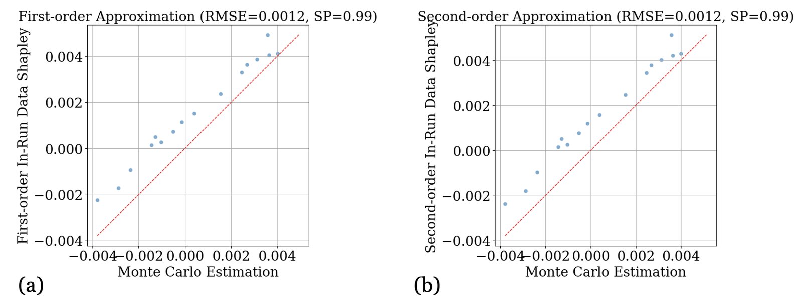
Figure 6: Comparison between the Monte Carlo-estimated In-Run Data Shapley and First/Second-order In-Run Data Shapley (learning rate ).
图 6:蒙特卡洛估计的 In-Run Data Shapley 与一/二阶 In-Run Data Shapley 的比较(学习率 )。
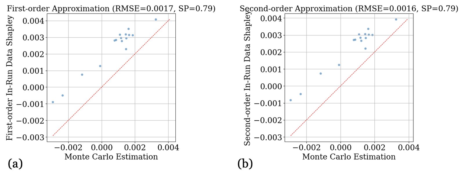
Figure 7: Comparison between the Monte Carlo-estimated In-Run Data Shapley and First/Second-order In-Run Data Shapley (learning rate ).
图 7:蒙特卡洛估计的 In-Run Data Shapley 与一/二阶 In-Run Data Shapley 的比较(学习率 )。
E.2.2 Approximation Error for Utility Function
In this experiment, we empirically investigate the errors of the first- and second-order approximations to on GPT2, as proposed in Section 4.1. The correlations are shown in Figure 8. As we can see, even the first-order approximation achieves a high approximation accuracy, and the inclusion of the second-order interaction term does not provide a notable improvement in accuracy.
E.2.2 效用函数的逼近误差
本实验经验考察第 4.1 节对 GPT2 上 的一、二阶逼近误差。相关见图 8。可见即便一阶逼近已达很高精度,纳入二阶交互项对精度并无显著提升。
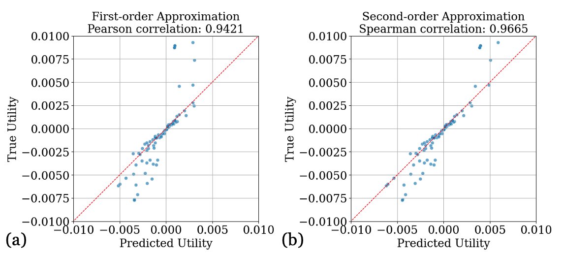
Figure 8: (a) We show the correlation between the ground-truth model validation loss change in one gradient update iteration and the first-order Taylor approximation. (b) We show the correlation between and the second-order approximation.
图 8:(a) 真实单步验证损失变化 与一阶 Taylor 逼近的相关。(b) 与二阶逼近的相关。
Remark 7(Difficulty in Extending to Adam).
The techniques developed in this section are specifically tailored for SGD. It is not directly extendable to other popular optimizers like Adam due to their normalization terms. Nonetheless, using SGD as a proxy for Adam allows for efficient data attribution, which is the approach we adopted in practice and has proved to be effective in our experiment. This provides a practical and effective solution for the current scope of our work. Extending these techniques to support Adam and similar optimizers remains an exciting direction for future research.
注记 7(扩展到 Adam 的困难)。
本节技术专为 SGD 定制,因归一化项而不能直接扩到 Adam 等流行优化器。不过用 SGD 作 Adam 的代理仍可高效做数据归因——这是我们实践中采用的做法,并在实验中证明有效,为当前工作范围提供了务实方案。扩展到 Adam 及类似优化器仍是有吸引力的未来方向。
E.3 Details about Section 5.3.1
In this experiment, we first conduct one training run for 20,000 iterations. Among all the corpus that has been used in the training, we compute their In-Run Data Shapley and filter out all corpus among this subset that has negative contributions to model training. After filtering out the 16% negative valued corpus, we train another model on the remaining dataset for 10,000 iterations with all hyperparameters staying the same.
本实验先做一次 20,000 步训练;在用过的全部语料上计算 In-Run Data Shapley,并滤掉对该子集训练有负贡献的语料。去掉 16% 负值语料后,在剩余数据上以相同超参再训 10,000 步。
Despite the Pile dataset undergoing multiple layers of data curation (Gao et al., 2020), we still find a significant amount of poor-quality corpus through In-Run Data Shapley. For example, we discovered a large amount of corpora in the PubMed Central domain that are simply empty spaces. Figure 9 provides two examples of the corpus that received the lowest In-Run Data Shapley scores. Additionally, we found several corpora with negative values that appear normal, which is likely due to a distribution shift with the validation corpus. Crafting a representative validation set is an important direction for future work.
尽管 Pile 已经过多层数据策展(Gao 等, 2020),我们仍通过 In-Run Data Shapley 发现大量劣质语料。例如 PubMed Central 领域中有大量几乎全是空格的语料。图 9 给出 In-Run Data Shapley 分数最低的两个语料示例。另有若干负值语料看起来正常,很可能因与验证语料存在分布偏移。如何构造有代表性的验证集是重要未来方向。
Corpus with meaningless numbers
,2,3,3,1,3,0,3,0,2,0,0, 0,0,0,0,0,0,0,0,0,0,2,0… 3,3,3,3,3,3,3,3,1,3,3,… 0,0,0,0,0,0,0,0,0,0,2,… 3,3,3,3,3,3,3,3,3,0,3,… 1,0,0,0,0,0,0,0,0,0,2,… 3,3,3,3,3,3,3,2,3,3,1,… 0,0,0,0,0,0,0,0,0,0,3,… 3,3,3,3,3,1,3,3,3,3,3,… 0,0,0,0,0,0,0,0,0,0,1,…
Figure 9: Examples of low-quality corpus in Pile found by In-Run Data Shapley. Left: a corpus with meaningless numbers. Right: a corpus with meaningless symbols (likely due to errors from web crawling.)
无意义数字的语料
,2,3,3,1,3,0,3,0,2,0,0, 0,0,0,0,0,0,0,0,0,0,2,0… 3,3,3,3,3,3,3,3,1,3,3,… 0,0,0,0,0,0,0,0,0,0,2,… 3,3,3,3,3,3,3,3,3,0,3,… 1,0,0,0,0,0,0,0,0,0,2,… 3,3,3,3,3,3,3,2,3,3,1,… 0,0,0,0,0,0,0,0,0,0,3,… 3,3,3,3,3,1,3,3,3,3,3,… 0,0,0,0,0,0,0,0,0,0,1,…
图 9:In-Run Data Shapley 在 Pile 中发现的低质语料示例。左:无意义数字语料。右:无意义符号语料(很可能来自网页抓取错误)。
E.3.1 Data selection performance on Pythia 410M
Figure 10 shows a performance comparison between the original training run and the model trained on the cleaned subsets on Pythia-410M. Similar to the results on GPT2, we can see that removing lower-quality data leads to a significantly faster drop in test loss compared to the original training run, highlighting the effectiveness of In-Run Data Shapley across different architectures.
E.3.1 Pythia 410M 上的数据选择表现
图 10 比较 Pythia-410M 上原训练与清洗子集训练的表现。与 GPT2 类似,去掉较低质量数据后测试损失下降显著更快,凸显 In-Run Data Shapley 跨不同架构的有效性。
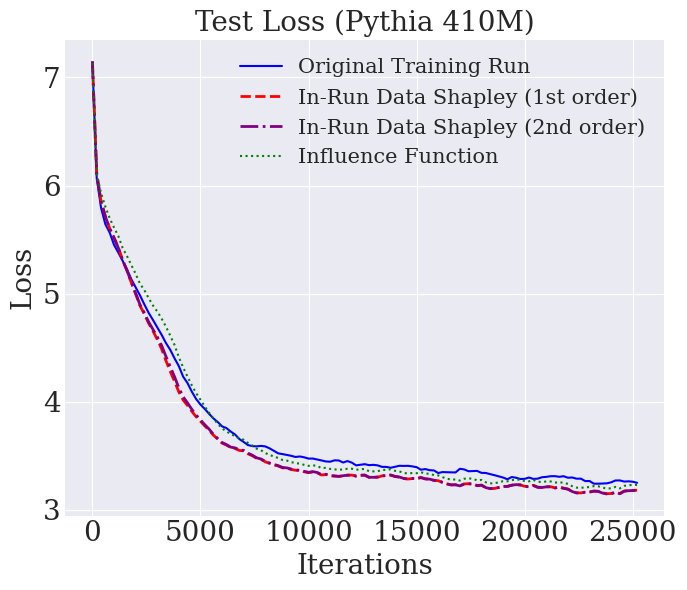
Figure 10: Test loss comparison between the original training run and model trained on the cleaned subset according to different data attribution techniques for Pythia-410M.
图 10:Pythia-410M 上原训练与按不同数据归因技术清洗子集后训练的测试损失比较。
E.4 Additional Results for Section 5.3.2
In addition to Figure 3, we also plot the average value scores of corpora from each domain, averaged across all corpora within the same domain that has been used in gradient updates, over the first 10,000 gradient update iterations. As training progresses, the magnitude of data value scores converges towards zero, which aligns with the diminishing returns property of neural network training. This indicates that the contribution of data points depends on the order in which they are used during training, an aspect that Retraining-based Data Shapley methods cannot capture. Data points introduced in later stages of training contribute less to model performance improvement.
除图 3 外,我们还绘制各领域语料的平均价值分数——对前 10,000 次梯度更新中用过的同领域语料取平均。随训练推进,数据价值分数的幅度趋向零,符合神经网络训练的收益递减。这表明数据点贡献取决于使用顺序——基于重训的 Data Shapley 无法捕捉这一点。训练后期引入的数据点对性能提升贡献更小。
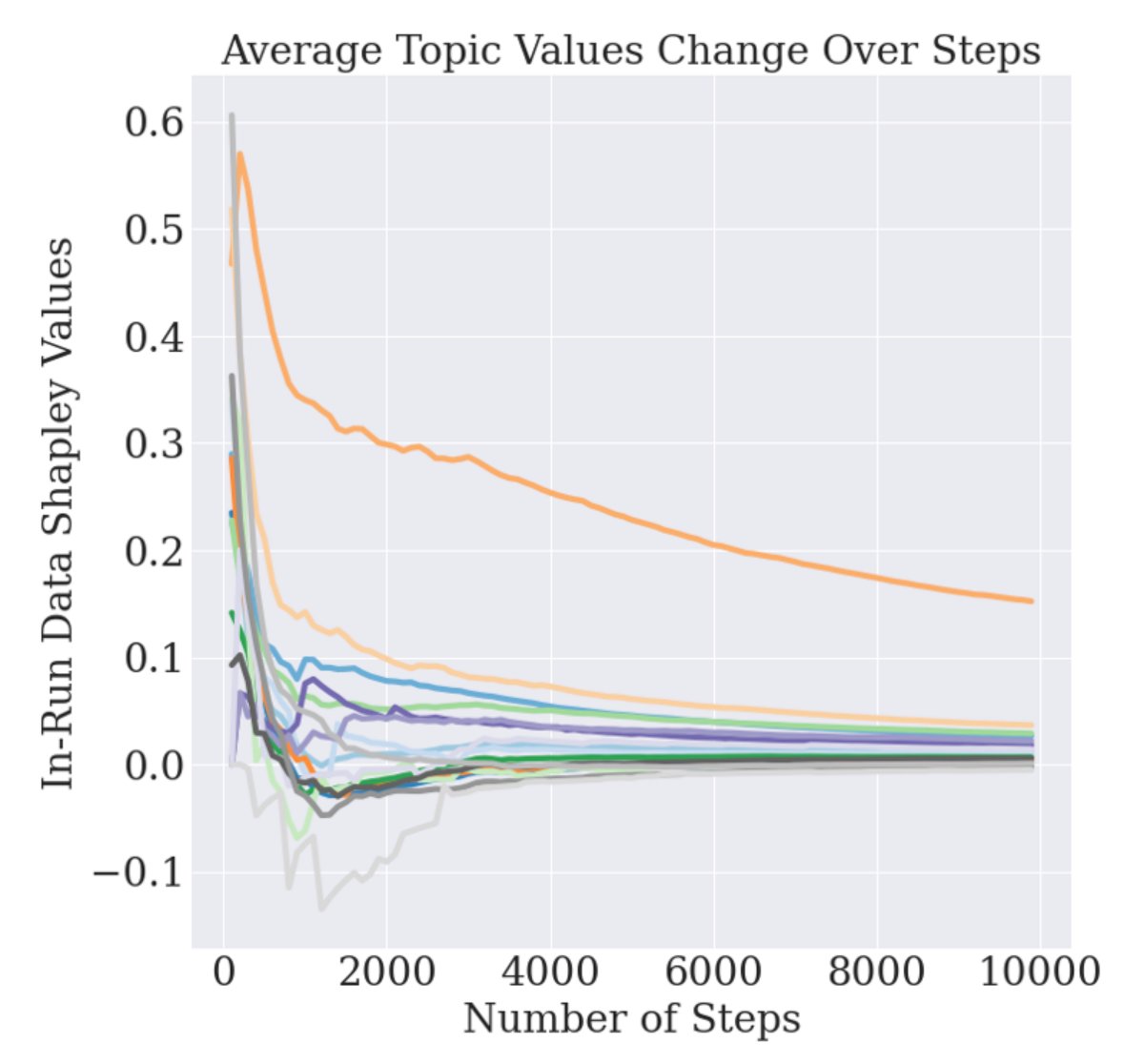
Figure 11: The change of average contribution for data points from each domain to a corpus of math text (same setting as Figure 3).
图 11:各领域数据点对某数学文本语料平均贡献的变化(设定同图 3)。
E.5 Details about Section 5.3.3
In Section 5.3.3, we use GPT-4 to generate varying levels of paraphrased versions of an original corpus from the training set, categorized as "Partial exactly the same," "Paraphrase," "Significant paraphrase," and "Similar topic." For "Partial exactly the same," the corpus is used as the answer in a creative writing instruction-answer pair. The specific prompt for prompting GPT-4 with examples of the full dialogue are shown in Figure 13, 14, 15. We generate 3 sets of corpus groups, and the experiment results are taken as the average. Figure 12 shows the distribution of calculated In-Run Data Shapley. As we can see, most corpora’s values are around 0, but certain corpora have significantly higher values than the other, which means their contributions are higher for the target validation corpus.
第 5.3.3 节中,我们用 GPT-4 对训练集中原始语料生成不同程度的改写,分为「部分完全相同」「改写」「大幅改写」「相似主题」。「部分完全相同」把该语料用作创意写作指令–答案对中的答案。提示 GPT-4 的具体提示与完整对话示例见图 13、14、15。我们生成 3 组语料群,实验结果取平均。图 12 显示算出的 In-Run Data Shapley 分布:多数语料价值约在 0 附近,但某些语料价值显著更高,意味着它们对目标验证语料贡献更大。
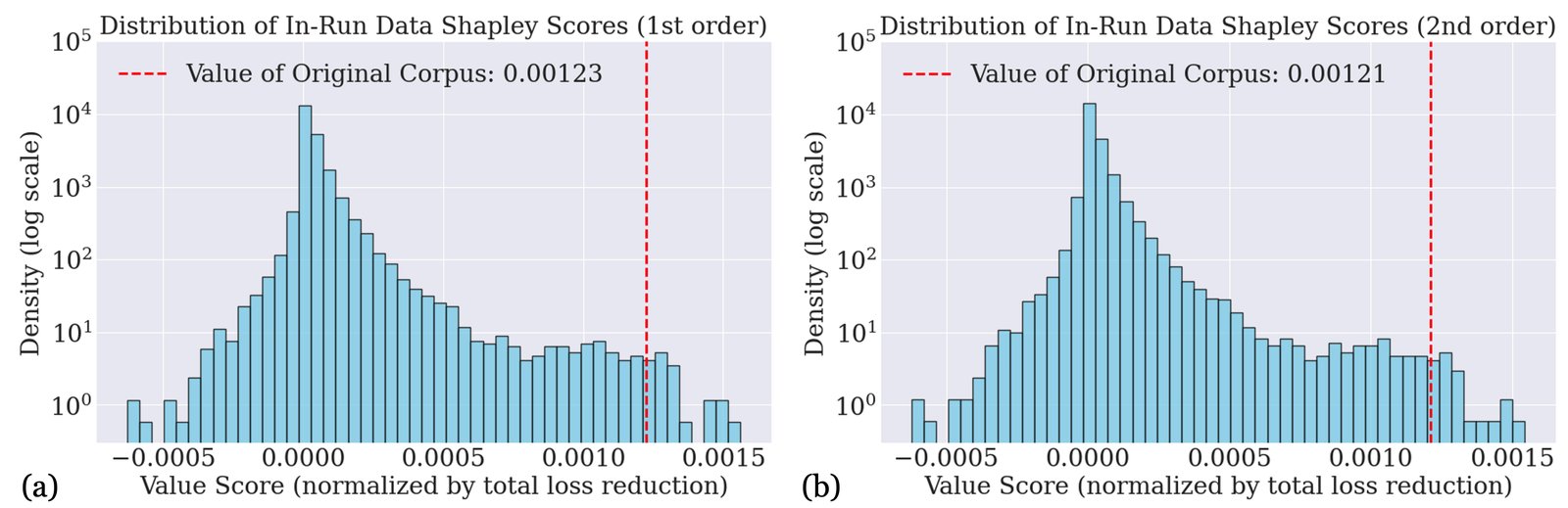
Figure 12: The distribution of calculated In-Run Data Shapley values.
图 12:算出的 In-Run Data Shapley 值分布。
Dialogue with GPT4 for generating corpus of varying levels of similarity (Original corpus from Wikipedia)
[Generate "Partial exactly the same"]
Instruction: [INSERT]
Answer: In 2012, Radhi recruited new ’musicians’ for OAG, who were selected from among the students of Akademi Seni Budaya dan Warisan Kebangsaan (). The new line-up consists ofe Qi Razali (drums/backing vocals - original drummer back to the drum position), Muhamad Nizam (guitar - since 2005), Nazrin Zabidi (bass guitar/backing vocals), and Izmer Khasbullah (keyboard/backing vocals). Radhi defines OAG’s new music as aslinatif, a combination of muzik asli or traditional music and alternative. Shortly after their reunion, they released the soundtrack and theme song to the TV series, Friday I’m in Love. Few other singles like Si Pengasih Muda, Di Bawah Tanah Ayer and Ambisi” are set to be released soon and also a full studio album coming afterwards.
Please help filling in [INSERT] as the instruction for a creative writing task.
Write a short story about Radhi and his band OAG as they recruit new members and blend traditional music with alternative sounds. Describe their creative challenges and successes leading up to their new releases.
[Generate "Paraphrase"]
Could you paraphrase the paragraph start from "In 2012, Radhi recruited …"?
In 2012, Radhi assembled new ’musicians’ for OAG, choosing from students at the Akademi Seni Budaya dan Warisan Kebangsaan. The updated lineup includes Qi Razali on drums and backing vocals, returning to his original role, along with Muhamad Nizam on guitar (since 2005), Nazrin Zabidi playing bass and providing backing vocals, and Izmer Khasbullah on keyboards and backing vocals. Radhi describes OAG’s revamped sound as ’aslinatif,’ a fusion of traditional (muzik asli) and alternative music. Following their reformation, they quickly launched the soundtrack and theme for the TV series "Friday I’m in Love." Upcoming releases include singles like "Si Pengasih Muda," "Di Bawah Tanah Ayer," and "Ambisi," along with a new studio album.
[Generate "Significant paraphrase"]
Could you make it less look like the original paragraph? Feel free to modify the sentences.
In 2012, Radhi selected a new set of musicians from the students of Akademi Seni Budaya dan Warisan Kebangsaan to join OAG. The band’s updated composition includes Qi Razali, who returned to his original role on drums and backing vocals, alongside Muhamad Nizam who has been on guitar since 2005, Nazrin Zabidi on bass with backing vocals, and Izmer Khasbullah playing the keyboard and adding backing vocals. Radhi has termed the band’s evolved musical expression as ’aslinatif,’ a blend of traditional and alternative sounds. Following their comeback, their first major project was producing the soundtrack and theme for the TV series "Friday I’m in Love." The band is also planning to launch several singles such as "Si Pengasih Muda," "Di Bawah Tanah Ayer," and "Ambisi," and is working towards a new full-length album.
[Generate "Similar topic"]
(COPY PREVIOUS INSTRUCTION-ANSWER PAIR) … The above is an example of instruction-answer pair of creative writing. Could you write an instruction-answer pair regarding a less similar but not completely irrelevant topic?
### Instruction: Write a short story about a classical violinist who decides to explore jazz music, detailing her first encounter with a jazz band. ### Answer: Elena, a classically trained violinist known for her precise and emotive performances, felt something was missing in her musical life. Curiosity led her to a dimly lit jazz club downtown, where the improvised rhythms and melodies captivated her. Hesitantly, she approached the band after their set, violin in hand. They invited her to join them for a jam session the following week. As she stepped onto the stage, her traditional techniques blended unexpectedly with the saxophonist’s smooth runs and the drummer’s rhythmic beats. The fusion of classical precision and jazz spontaneity created a thrilling new sound. Elena found herself reinvigorated, her violin singing with a freedom she had never before experienced.
Figure 13: Our dialogue with GPT4 for generating corpus of varying levels of similarity for the original corpus from Wikipedia.
与 GPT-4 生成不同相似度语料的对话(原始语料来自 Wikipedia)
[生成「部分完全相同」]
Instruction: [INSERT]
Answer: In 2012, Radhi recruited new 'musicians' for OAG, who were selected from among the students of Akademi Seni Budaya dan Warisan Kebangsaan (). The new line-up consists ofe Qi Razali (drums/backing vocals - original drummer back to the drum position), Muhamad Nizam (guitar - since 2005), Nazrin Zabidi (bass guitar/backing vocals), and Izmer Khasbullah (keyboard/backing vocals). Radhi defines OAG's new music as aslinatif, a combination of muzik asli or traditional music and alternative. Shortly after their reunion, they released the soundtrack and theme song to the TV series, Friday I'm in Love. Few other singles like Si Pengasih Muda, Di Bawah Tanah Ayer and Ambisi" are set to be released soon and also a full studio album coming afterwards.
请帮助把 [INSERT] 填成创意写作任务的指令。
Write a short story about Radhi and his band OAG as they recruit new members and blend traditional music with alternative sounds. Describe their creative challenges and successes leading up to their new releases.
[生成「改写」]
Could you paraphrase the paragraph start from "In 2012, Radhi recruited …"?
In 2012, Radhi assembled new 'musicians' for OAG, choosing from students at the Akademi Seni Budaya dan Warisan Kebangsaan. The updated lineup includes Qi Razali on drums and backing vocals, returning to his original role, along with Muhamad Nizam on guitar (since 2005), Nazrin Zabidi playing bass and providing backing vocals, and Izmer Khasbullah on keyboards and backing vocals. Radhi describes OAG's revamped sound as 'aslinatif,' a fusion of traditional (muzik asli) and alternative music. Following their reformation, they quickly launched the soundtrack and theme for the TV series "Friday I'm in Love." Upcoming releases include singles like "Si Pengasih Muda," "Di Bawah Tanah Ayer," and "Ambisi," along with a new studio album.
[生成「大幅改写」]
Could you make it less look like the original paragraph? Feel free to modify the sentences.
In 2012, Radhi selected a new set of musicians from the students of Akademi Seni Budaya dan Warisan Kebangsaan to join OAG. The band's updated composition includes Qi Razali, who returned to his original role on drums and backing vocals, alongside Muhamad Nizam who has been on guitar since 2005, Nazrin Zabidi on bass with backing vocals, and Izmer Khasbullah playing the keyboard and adding backing vocals. Radhi has termed the band's evolved musical expression as 'aslinatif,' a blend of traditional and alternative sounds. Following their comeback, their first major project was producing the soundtrack and theme for the TV series "Friday I'm in Love." The band is also planning to launch several singles such as "Si Pengasih Muda," "Di Bawah Tanah Ayer," and "Ambisi," and is working towards a new full-length album.
[生成「相似主题」]
(COPY PREVIOUS INSTRUCTION-ANSWER PAIR) … The above is an example of instruction-answer pair of creative writing. Could you write an instruction-answer pair regarding a less similar but not completely irrelevant topic?
### Instruction: Write a short story about a classical violinist who decides to explore jazz music, detailing her first encounter with a jazz band. ### Answer: Elena, a classically trained violinist known for her precise and emotive performances, felt something was missing in her musical life. Curiosity led her to a dimly lit jazz club downtown, where the improvised rhythms and melodies captivated her. Hesitantly, she approached the band after their set, violin in hand. They invited her to join them for a jam session the following week. As she stepped onto the stage, her traditional techniques blended unexpectedly with the saxophonist's smooth runs and the drummer's rhythmic beats. The fusion of classical precision and jazz spontaneity created a thrilling new sound. Elena found herself reinvigorated, her violin singing with a freedom she had never before experienced.
图 13:我们与 GPT-4 的对话,用于为 Wikipedia 原始语料生成不同相似度等级的语料。
Example Dialogue with GPT4 for generating corpus of varying levels of similarity (Original corpus from CNN)
[Generate "Partial exactly the same"]
Instruction: [INSERT]
Answer: The morning after Obama’s win, The New York Times declared "Racial Barrier Falls in Decisive Victory." The Los Angeles Times asserted that "for the first time in human history, a largely white nation has elected a black man to be its paramount leader." Some black commentators openly wept on election night, thrilled with witnessing the election of our first black president. Even Sen. John McCain, conceding defeat, pointed to the greatness of the American promise fulfilled in the election of his opponent. Obama’s victory offered the possibility that the scars of America’s racial legacy were healed or, at least, that they were less raw.
Please help filling in [INSERT] as the instruction for a creative writing task.
Write a reflective essay on the significance of Barack Obama’s 2008 presidential election victory, focusing on its impact on race relations in the United States and the emotional responses it elicited from different communities.
[Generate "Paraphrase"]
Could you paraphrase the paragraph?
The morning after Obama’s victory, The New York Times proclaimed "Racial Barrier Falls in Decisive Victory," while The Los Angeles Times noted that "for the first time in human history, a predominantly white nation has elected a black man as its paramount leader." Some black commentators wept openly on election night, overjoyed at witnessing the election of the first black president. Even Sen. John McCain, in his concession speech, highlighted the fulfillment of the American promise through his opponent’s win. Obama’s triumph suggested the possibility that the deep wounds of America’s racial history were healing or, at the very least, becoming less acute.
[Generate "Significant paraphrase"]
Could you make it less look like the original paragraph? Feel free to modify the sentences.
The morning after Obama’s victory, headlines captured the historic moment: The New York Times announced "Racial Barrier Falls in Decisive Victory," and The Los Angeles Times highlighted that "for the first time, a predominantly white nation has chosen a black man as its leader." On election night, many black commentators shed tears of joy, moved by the milestone of electing the first black president. Even Sen. John McCain, in his concession speech, acknowledged the realization of the American promise in his opponent’s success. Obama’s win signaled a potential healing of America’s racial wounds or at least a step toward easing their pain.
[Generate "Similar topic"]
(COPY PREVIOUS INSTRUCTION-ANSWER PAIR) … The above is an example of instruction-answer pair of creative writing. Could you write an instruction-answer pair regarding a less similar but not completely irrelevant topic?
### Instruction: Write a reflective essay on the significance of the Supreme Court’s 2015 decision to legalize same-sex marriage nationwide, focusing on its impact on LGBTQ+ rights in the United States and the emotional responses it elicited from different communities.
Answer: The morning after the Supreme Court’s landmark decision, The New York Times declared "Equal Dignity in the Eyes of the Law." The Washington Post highlighted, "Love Wins: Supreme Court Affirms Same-Sex Marriage Nationwide." Many in the LGBTQ+ community celebrated with tears of joy, feeling validated and recognized. Even some of the justices who dissented acknowledged the profound impact of the decision on American society. The ruling represented a major milestone in the fight for LGBTQ+ rights, symbolizing a shift toward greater acceptance and equality.
Figure 14: Our dialogue with GPT4 for generating corpus of varying levels of similarity for the original corpus from a CNN news.
与 GPT-4 生成不同相似度语料的示例对话(原始语料来自 CNN)
[生成「部分完全相同」]
Instruction: [INSERT]
Answer: The morning after Obama's win, The New York Times declared "Racial Barrier Falls in Decisive Victory." The Los Angeles Times asserted that "for the first time in human history, a largely white nation has elected a black man to be its paramount leader." Some black commentators openly wept on election night, thrilled with witnessing the election of our first black president. Even Sen. John McCain, conceding defeat, pointed to the greatness of the American promise fulfilled in the election of his opponent. Obama's victory offered the possibility that the scars of America's racial legacy were healed or, at least, that they were less raw.
请帮助把 [INSERT] 填成创意写作任务的指令。
Write a reflective essay on the significance of Barack Obama's 2008 presidential election victory, focusing on its impact on race relations in the United States and the emotional responses it elicited from different communities.
[生成「改写」]
Could you paraphrase the paragraph?
The morning after Obama's victory, The New York Times proclaimed "Racial Barrier Falls in Decisive Victory," while The Los Angeles Times noted that "for the first time in human history, a predominantly white nation has elected a black man as its paramount leader." Some black commentators wept openly on election night, overjoyed at witnessing the election of the first black president. Even Sen. John McCain, in his concession speech, highlighted the fulfillment of the American promise through his opponent's win. Obama's triumph suggested the possibility that the deep wounds of America's racial history were healing or, at the very least, becoming less acute.
[生成「大幅改写」]
Could you make it less look like the original paragraph? Feel free to modify the sentences.
The morning after Obama's victory, headlines captured the historic moment: The New York Times announced "Racial Barrier Falls in Decisive Victory," and The Los Angeles Times highlighted that "for the first time, a predominantly white nation has chosen a black man as its leader." On election night, many black commentators shed tears of joy, moved by the milestone of electing the first black president. Even Sen. John McCain, in his concession speech, acknowledged the realization of the American promise in his opponent's success. Obama's win signaled a potential healing of America's racial wounds or at least a step toward easing their pain.
[生成「相似主题」]
(COPY PREVIOUS INSTRUCTION-ANSWER PAIR) … The above is an example of instruction-answer pair of creative writing. Could you write an instruction-answer pair regarding a less similar but not completely irrelevant topic?
### Instruction: Write a reflective essay on the significance of the Supreme Court's 2015 decision to legalize same-sex marriage nationwide, focusing on its impact on LGBTQ+ rights in the United States and the emotional responses it elicited from different communities.
Answer: The morning after the Supreme Court's landmark decision, The New York Times declared "Equal Dignity in the Eyes of the Law." The Washington Post highlighted, "Love Wins: Supreme Court Affirms Same-Sex Marriage Nationwide." Many in the LGBTQ+ community celebrated with tears of joy, feeling validated and recognized. Even some of the justices who dissented acknowledged the profound impact of the decision on American society. The ruling represented a major milestone in the fight for LGBTQ+ rights, symbolizing a shift toward greater acceptance and equality.
图 14:我们与 GPT-4 的对话,用于为 CNN 新闻原始语料生成不同相似度等级的语料。
Example Dialogue with GPT4 for generating corpus of varying levels of similarity (Original corpus from princeton.edu)
[Generate "Partial exactly the same"]
Instruction: [INSERT]
Answer: The process was purchased by the German chemical company BASF (a coal tar dye supplier), which assigned Carl Bosch the difficult task of scaling up Haber’s tabletop machine to industrial-level production.Haber and Bosch were later awarded Nobel prizes, in 1918 and 1931 respectively, for their work in overcoming the chemical and engineering problems posed by the use of large-scale, continuous-flow, high-pressure technology.
Please help filling in [INSERT] as the instruction for a creative writing task.
Write a short story or essay about Carl Bosch’s efforts to scale up Haber’s tabletop machine to industrial production. Highlight the scientific and engineering challenges he faced, the solutions he found, and the impact of his work on society. Include historical context and personal anecdotes.
[Generate "Paraphrase"]
Could you paraphrase the paragraph?
The German chemical company BASF, known for supplying coal tar dyes, acquired the process and tasked Carl Bosch with the challenging job of scaling Haber’s small-scale machine to an industrial level. Haber and Bosch were eventually honored with Nobel prizes in 1918 and 1931, respectively, for their breakthroughs in addressing the chemical and engineering difficulties associated with large-scale, continuous-flow, high-pressure technology.
[Generate "Significant paraphrase"]
Could you make it less look like the original paragraph? Feel free to modify the sentences.
BASF, a German firm specializing in coal tar dyes, took on the task and brought in Carl Bosch to scale up Haber’s experimental setup to an industrial scale. Bosch faced numerous challenges but ultimately succeeded. Their groundbreaking work in developing large-scale, high-pressure technology earned them Nobel Prizes, with Haber being recognized in 1918 and Bosch in 1931.
[Generate "Similar topic"]
(COPY PREVIOUS INSTRUCTION-ANSWER PAIR) … The above is an example of instruction-answer pair of creative writing. Could you write an instruction-answer pair regarding a less similar but not completely irrelevant topic?
### Instruction: Write a short story or essay about the development of the polio vaccine by Jonas Salk. Focus on the scientific challenges he faced, the innovative methods he used, and the impact of the vaccine on public health. Include historical context and personal anecdotes.
Answer: In the early 1950s, Jonas Salk embarked on a mission to develop a vaccine for polio, a disease that was causing widespread fear and paralysis. Salk faced significant scientific challenges, including finding a way to grow the poliovirus in large quantities and then inactivating it without destroying its ability to induce immunity.
Salk’s innovative method involved using formaldehyde to kill the virus while preserving its structure. After rigorous testing, the vaccine was declared safe and effective in 1955. This breakthrough led to mass vaccination campaigns, dramatically reducing polio incidence worldwide.
The impact of Salk’s vaccine was profound, turning a once-dreaded disease into a preventable condition. Salk’s work not only saved countless lives but also demonstrated the power of scientific innovation in overcoming public health challenges. His dedication and perseverance remain an inspiration in the field of medical research.
Figure 15: Our dialogue with GPT4 for generating corpus of varying levels of similarity for the original corpus from princeton.edu.
与 GPT-4 生成不同相似度语料的示例对话(原始语料来自 princeton.edu)
[生成「部分完全相同」]
Instruction: [INSERT]
Answer: The process was purchased by the German chemical company BASF (a coal tar dye supplier), which assigned Carl Bosch the difficult task of scaling up Haber's tabletop machine to industrial-level production.Haber and Bosch were later awarded Nobel prizes, in 1918 and 1931 respectively, for their work in overcoming the chemical and engineering problems posed by the use of large-scale, continuous-flow, high-pressure technology.
请帮助把 [INSERT] 填成创意写作任务的指令。
Write a short story or essay about Carl Bosch's efforts to scale up Haber's tabletop machine to industrial production. Highlight the scientific and engineering challenges he faced, the solutions he found, and the impact of his work on society. Include historical context and personal anecdotes.
[生成「改写」]
Could you paraphrase the paragraph?
The German chemical company BASF, known for supplying coal tar dyes, acquired the process and tasked Carl Bosch with the challenging job of scaling Haber's small-scale machine to an industrial level. Haber and Bosch were eventually honored with Nobel prizes in 1918 and 1931, respectively, for their breakthroughs in addressing the chemical and engineering difficulties associated with large-scale, continuous-flow, high-pressure technology.
[生成「大幅改写」]
Could you make it less look like the original paragraph? Feel free to modify the sentences.
BASF, a German firm specializing in coal tar dyes, took on the task and brought in Carl Bosch to scale up Haber's experimental setup to an industrial scale. Bosch faced numerous challenges but ultimately succeeded. Their groundbreaking work in developing large-scale, high-pressure technology earned them Nobel Prizes, with Haber being recognized in 1918 and Bosch in 1931.
[生成「相似主题」]
(COPY PREVIOUS INSTRUCTION-ANSWER PAIR) … The above is an example of instruction-answer pair of creative writing. Could you write an instruction-answer pair regarding a less similar but not completely irrelevant topic?
### Instruction: Write a short story or essay about the development of the polio vaccine by Jonas Salk. Focus on the scientific challenges he faced, the innovative methods he used, and the impact of the vaccine on public health. Include historical context and personal anecdotes.
Answer: In the early 1950s, Jonas Salk embarked on a mission to develop a vaccine for polio, a disease that was causing widespread fear and paralysis. Salk faced significant scientific challenges, including finding a way to grow the poliovirus in large quantities and then inactivating it without destroying its ability to induce immunity.
Salk's innovative method involved using formaldehyde to kill the virus while preserving its structure. After rigorous testing, the vaccine was declared safe and effective in 1955. This breakthrough led to mass vaccination campaigns, dramatically reducing polio incidence worldwide.
The impact of Salk's vaccine was profound, turning a once-dreaded disease into a preventable condition. Salk's work not only saved countless lives but also demonstrated the power of scientific innovation in overcoming public health challenges. His dedication and perseverance remain an inspiration in the field of medical research.
图 15:我们与 GPT-4 的对话,用于为 princeton.edu 原始语料生成不同相似度等级的语料。
E.5.1 Additional Experiment: Relevant Domain Detection
In this additional experiment, we evaluate the effectiveness of different data attribution techniques in identifying relevant domain-specific corpora within the Pile dataset. Specifically, we take a random batch of the validation corpus from sub-domains of the Pile dataset and evaluate the normalized recall@1000 scores. This metric measures the proportion of same-domain corpora as the validation corpora among the 1000 highest-valued corpora, normalized by the global proportion of this domain within the Pile dataset. As shown in Table 3, BM25 performs well on this task in general. Both the first-order and second-order In-Run Data Shapley methods outperform the influence function in detecting relevant domain corpora. Analysis: The influence function only uses information from the final trained models, which can result in highly noisy value scores since the removal of one training data point might have a negligible effect on the final model performance. In contrast, In-Run Data Shapley effectively leverages information from all intermediate checkpoints during model training, providing a more comprehensive and accurate assessment of each data point’s value. While BM25 performs well on most of the domains, there are still cases where In-Run Data Shapley achieves better detection rate, which implies that gradient information may be more useful in determining semantic similarity to some extent.
E.5.1 补充实验:相关领域检测
本补充实验评估不同数据归因技术在 Pile 中识别相关领域语料的效果。具体地,从 Pile 各子域随机取一批验证语料,评估归一化 recall@1000:在价值最高的 1000 条语料中,与验证语料同域的比例,再除以该域在 Pile 中的全局比例。如表 3,BM25 整体表现不错;一、二阶 In-Run Data Shapley 在检测相关领域语料上均优于影响函数。分析: 影响函数只用最终已训模型信息,去掉单点对最终表现影响可能微乎其微,价值分数噪声很大;In-Run Data Shapley 有效利用训练全程中间检查点信息,对每点价值评估更全面准确。虽 BM25 在多数领域表现好,仍有 In-Run Data Shapley 检测率更高的情形,暗示梯度信息在一定程度上对判定语义相似度更有用。
| Github | EuroParl | ArXiv | PhilPapers | FreeLaw | HackerNews | StackExchange | Wikipedia (en) | |
|---|---|---|---|---|---|---|---|---|
| In-Run Data Shapley (1st order) | 30.5 | 12.7 | 48.4 | 0.6 | 14.6 | 2.7 | 16.3 | 14.5 |
| In-Run Data Shapley (2nd order) | 29 | 14.8 | 50 | 0.4 | 16.9 | 3.8 | 20 | 18.9 |
| Influence Function | 17.9 | 4.1 | 41.7 | 0.5 | 5.7 | 2.6 | 6.5 | 5.5 |
| BM25 | 18.8 | 6.3 | 44.8 | 1.1 | 72.6 | 9.9 | 37.2 | 18.6 |
| PubMed Abstracts | USPTO Backgrounds | PubMed Central | Enron Emails | NIH ExPorter | DM Mathematics | Ubuntu IRC | Gutenberg (PG-19) | |
| In-Run Data Shapley (1st order) | 10.4 | 10.5 | 30 | 0.8 | 1.7 | 23.5 | 10.2 | 8.7 |
| In-Run Data Shapley (2nd order) | 16.6 | 11.1 | 31.1 | 1 | 1.9 | 24.5 | 11.5 | 15.3 |
| Influence Function | 10.2 | 7.4 | 26.9 | 0.2 | 1.2 | 10.1 | 4.3 | 8.8 |
| BM25 | 28.6 | 23 | 53.7 | 1 | 4.1 | 34.6 | 12.5 | 25.9 |
Table 3: Results of relevant domain corpus detection experiment, where the metric is the normalized recall@1000 (i.e., the proportion of the same domain corpora as the validation corpora among the 1000 corpora with the highest values, normalized by the global proportion of this domain among the Pile dataset).
| Github | EuroParl | ArXiv | PhilPapers | FreeLaw | HackerNews | StackExchange | Wikipedia (en) | |
|---|---|---|---|---|---|---|---|---|
| In-Run Data Shapley(一阶) | 30.5 | 12.7 | 48.4 | 0.6 | 14.6 | 2.7 | 16.3 | 14.5 |
| In-Run Data Shapley(二阶) | 29 | 14.8 | 50 | 0.4 | 16.9 | 3.8 | 20 | 18.9 |
| 影响函数 | 17.9 | 4.1 | 41.7 | 0.5 | 5.7 | 2.6 | 6.5 | 5.5 |
| BM25 | 18.8 | 6.3 | 44.8 | 1.1 | 72.6 | 9.9 | 37.2 | 18.6 |
| PubMed Abstracts | USPTO Backgrounds | PubMed Central | Enron Emails | NIH ExPorter | DM Mathematics | Ubuntu IRC | Gutenberg (PG-19) | |
| In-Run Data Shapley(一阶) | 10.4 | 10.5 | 30 | 0.8 | 1.7 | 23.5 | 10.2 | 8.7 |
| In-Run Data Shapley(二阶) | 16.6 | 11.1 | 31.1 | 1 | 1.9 | 24.5 | 11.5 | 15.3 |
| 影响函数 | 10.2 | 7.4 | 26.9 | 0.2 | 1.2 | 10.1 | 4.3 | 8.8 |
| BM25 | 28.6 | 23 | 53.7 | 1 | 4.1 | 34.6 | 12.5 | 25.9 |
表 3:相关领域语料检测实验结果,指标为归一化 recall@1000(即价值最高的 1000 条中与验证语料同域的比例,再按该域在 Pile 中的全局比例归一化)。
Original Wikipedia Corpus
In 2012, Radhi recruited new ’musicians’ for OAG, who were selected from among the students of Akademi Seni Budaya dan Warisan Kebangsaan (). The new line-up consists of Qi Razali (drums/backing vocals - original drummer …
A corpus that is partially same
Instruction: Write a short story about Radhi and his band OAG as they recruit new members and blend traditional music with alternative sounds. Describe their creative challenges and successes leading up to their new releases. ### Answer: In 2012, Radhi recruited new ’musicians’ for OAG, who were selected from among the students of Akademi Seni Budaya dan Warisan Kebangsaan (). The new line-up consists of Qi Razali (drums/backing vocals - original drummer …
原始 Wikipedia 语料
In 2012, Radhi recruited new 'musicians' for OAG, who were selected from among the students of Akademi Seni Budaya dan Warisan Kebangsaan (). The new line-up consists of Qi Razali (drums/backing vocals - original drummer …
部分相同的语料
Instruction: Write a short story about Radhi and his band OAG as they recruit new members and blend traditional music with alternative sounds. Describe their creative challenges and successes leading up to their new releases. ### Answer: In 2012, Radhi recruited new 'musicians' for OAG, who were selected from among the students of Akademi Seni Budaya dan Warisan Kebangsaan (). The new line-up consists of Qi Razali (drums/backing vocals - original drummer …
Original Wikipedia Corpus
In 2012, Radhi recruited new ’musicians’ for OAG, who were selected from among the students of Akademi Seni Budaya dan Warisan Kebangsaan (). The new line-up consists of Qi Razali (drums/backing vocals - original drummer …
Synthetic "Similar topic" Corpus
Instruction: Write a short story about a classical violinist who decides to explore jazz music, detailing her first encounter with a jazz band. ### Answer: Elena, a classically trained violinist known for her precise and emotive performances …
原始 Wikipedia 语料
In 2012, Radhi recruited new 'musicians' for OAG, who were selected from among the students of Akademi Seni Budaya dan Warisan Kebangsaan (). The new line-up consists of Qi Razali (drums/backing vocals - original drummer …
合成「相似主题」语料
Instruction: Write a short story about a classical violinist who decides to explore jazz music, detailing her first encounter with a jazz band. ### Answer: Elena, a classically trained violinist known for her precise and emotive performances …
E.6 Comparison with other data attribution baselines on small-scale models
In this section, we evaluate In-Run Data Shapley using standard benchmarks for data attribution techniques, including mislabeled data detection and data selection. While data attribution scores can generally indicate data quality, they are not specifically optimized for these benchmarks. Furthermore, approximating the Shapley value has intrinsic merit beyond these standard tasks (e.g., for royalty sharing of AI-generated contents (Wang et al., 2024a)). As such, this evaluation primarily serves as a sanity check to confirm that In-Run Data Shapley can reasonably reflect data values. However, state-of-the-art performance is not expected since the method is not designed specifically for these tasks.
本节用数据归因技术的标准基准——包括错标检测与数据选择——评估 In-Run Data Shapley。虽归因分数一般可指示数据质量,但并非专为这些基准优化;且逼近 Shapley 值本身在这些标准任务之外也有内在价值(例如 AI 生成内容的版税分成(Wang 等, 2024a))。因此本评估主要作为健全性检查,确认 In-Run Data Shapley 能合理反映数据价值;因方法并非专为这些任务设计,不期望达到最先进表现。
We compare In-Run Data Shapley with several data attribution baselines, including Retraining-based Data Shapley (Ghorbani & Zou, 2019), KNN-Shapley (Jia et al., 2019a), influence function (Koh & Liang, 2017), Trak (Park et al., 2023), Empirical Influence Functions (Feldman & Zhang, 2020), and Datamodels (Ilyas et al., 2022). We also compare with LESS (Xia et al., 2024), an extension of TracIN-CP tailored for instruction tuning data selection.
我们把 In-Run Data Shapley 与若干数据归因基线比较,包括基于重训的 Data Shapley(Ghorbani & Zou, 2019)、KNN-Shapley(Jia 等, 2019a)、影响函数(Koh & Liang, 2017)、Trak(Park 等, 2023)、经验影响函数(Feldman & Zhang, 2020)与 Datamodels(Ilyas 等, 2022)。也与 LESS(Xia 等, 2024)比较——它是面向指令微调数据选择的 TracIN-CP 扩展。
As some baselines here require multiple model retrainings, we use a subset of 1,000 samples from CIFAR10 and ResNet18 architecture. We evaluate these techniques on two standard tasks for assessing data attribution methods: mislabeled data detection and data selection. We note that recent work (Wang et al., 2024d) questions the suitability of data attribution for data selection, but we include this metric due to its prevalence in existing literature.
因部分基线需多次模型重训,我们使用 CIFAR10 的 1,000 样本子集与 ResNet18 架构。在两个标准任务上评估:错标检测与数据选择。我们注意到近期工作(Wang 等, 2024d)质疑数据归因是否适于数据选择,但因该指标在既有文献中常见,仍予纳入。
Experiment settings.
We use ImageNet-pretrained ResNet18 as the architecture in the experiment. We use Adam with a learning rate 0.001, weight decay of 1e-4, and label smoothing of 0.1 over 50 epochs. The learning rate is reduced by a factor of 0.1 every 10 epochs. The batch size is set to 64. For retraining-based techniques (Retraining-based Data Shapley, Empirical Influence Functions, Datamodels), we estimate the corresponding attribution scores with 1000 model training runs. For LESS, we use the checkpoints from epochs 10, 20, 30, 40, 50 and set the projection dimension to 2048 as recommended in the original paper. For Trak, we set the projection dimension to be 2048. For KNN-Shapley, we set K=5 and use the features extracted from the last linear layer of ResNet18. We also evaluate its performance by averaging the results using the last checkpoints where .
实验设定。
架构为 ImageNet 预训练的 ResNet18。优化器用 Adam,学习率 0.001,权重衰减 1e-4,标签平滑 0.1,共 50 个 epoch;每 10 个 epoch 学习率乘 0.1;批大小 64。对基于重训的技术(基于重训的 Data Shapley、经验影响函数、Datamodels),用 1000 次模型训练估计归因分数。对 LESS,用第 10、20、30、40、50 个 epoch 的检查点,投影维按原文建议取 2048。对 Trak,投影维也取 2048。对 KNN-Shapley,取 K=5,特征来自 ResNet18 最后线性层;并评估对最后 个检查点取平均的结果,。
Mislabeled data detection.
The results in Table 4 show that KNN-Shapley achieves the highest performance in mislabeled data detection, likely due to its sensitivity to label changes. Retraining-based approaches (Retraining-based Data Shapley, Empirical Influence Functions, Datamodel) have the lowest performance, which can be attributed to Monte Carlo sample inefficiency and stochasticity during retraining, as noted in Wang & Jia (2023a). Among techniques requiring only one training run, Trak does not outperform others, aligning with observations in its original paper (Park et al., 2023) that ensembles are often necessary for high performance. LESS achieves better results by incorporating more information from intermediate checkpoints. In-Run Data Shapley and influence function achieve comparable performance, outperforming all other techniques except KNN-Shapley. The relatively high performance of In-Run Data Shapley is likely due to its deterministic estimation algorithm. Furthermore, it makes use of the information from all intermediate checkpoints.
错标数据检测。
表 4 显示 KNN-Shapley 在错标检测上表现最高,或因其对标签变化敏感。基于重训的方法(基于重训的 Data Shapley、经验影响函数、Datamodel)表现最低,可归因于蒙特卡洛样本效率低与重训随机性,如 Wang & Jia (2023a) 所指出。在只需一次训练的技术中,Trak 未优于其他,与原论文(Park 等, 2023)中常需集成才能高性能的观察一致。LESS 因纳入更多中间检查点信息而更好。In-Run Data Shapley 与影响函数表现相当,优于除 KNN-Shapley 外的所有技术。In-Run Data Shapley 相对较高的表现或因其确定性估计算法,并利用了全部中间检查点信息。
Data selection.
Table 5 shows that KNN-Shapley again excels when the selection budget is small. Interestingly, most data attribution techniques perform worse than random baseline for small selection budgets, aligning with observations that selecting data points solely based on attribution scores can harm dataset diversity (Wang et al., 2024d). For larger selection budgets (60%, 80%), single-training-run techniques achieve similar performance levels.
数据选择。
表 5 显示选择预算较小时 KNN-Shapley 再次领先。有趣的是,多数数据归因技术在小预算下差于随机基线,与「仅按归因分数选点会伤害数据集多样性」的观察一致(Wang 等, 2024d)。在更大选择预算(60%、80%)下,单次训练技术达到相近表现水平。
| Retraining-based Data Shapley (Ghorbani & Zou, 2019) | Empirical Influence Function (Feldman & Zhang, 2020) | Datamodels (Ilyas et al., 2022) |
|---|---|---|
| 0.582 (0.029) | 0.552 (0.017) | 0.52 (0.008) |
| KNN-Shapley (Jia et al., 2019a; Wang & Jia, 2023c) | Influence function (Koh & Liang, 2017) | LESS (Xia et al., 2024) |
| 0.76 (0.018) | 0.654 (0.054) | 0.55 (0.032) |
| 1st Order In-Run Data Shapley (ours) | 2nd Order In-Run Data Shapley (ours) | Trak (1 cpt) (Park et al., 2023) |
| 0.678 (0.045) | 0.680 (0.048) | 0.511 (0.012) |
| Trak (5 cpts) (Park et al., 2023) | Trak (15 cpts) (Park et al., 2023) | Trak (25 cpts) (Park et al., 2023) |
| 0.542 (0.025) | 0.609 (0.028) | 0.617 (0.021) |
Table 4: AUROC scores of mislabeled data detection task with various data attribution techniques on CIFAR10 dataset. The higher the AUROC score is, the better the method is. The results are across three different training runs (the randomness comes from construction of corrupted datasets), where we show the standard deviation in (). Methods with top-3 performance are bolded.
| 基于重训的 Data Shapley(Ghorbani & Zou, 2019) | 经验影响函数(Feldman & Zhang, 2020) | Datamodels(Ilyas 等, 2022) |
|---|---|---|
| 0.582 (0.029) | 0.552 (0.017) | 0.52 (0.008) |
| KNN-Shapley(Jia 等, 2019a;Wang & Jia, 2023c) | 影响函数(Koh & Liang, 2017) | LESS(Xia 等, 2024) |
| 0.76 (0.018) | 0.654 (0.054) | 0.55 (0.032) |
| 一阶 In-Run Data Shapley(本文) | 二阶 In-Run Data Shapley(本文) | Trak(1 检查点)(Park 等, 2023) |
| 0.678 (0.045) | 0.680 (0.048) | 0.511 (0.012) |
| Trak(5 检查点)(Park 等, 2023) | Trak(15 检查点)(Park 等, 2023) | Trak(25 检查点)(Park 等, 2023) |
| 0.542 (0.025) | 0.609 (0.028) | 0.617 (0.021) |
表 4:CIFAR10 上多种数据归因技术在错标检测任务的 AUROC。AUROC 越高越好。结果跨三次不同训练运行(随机性来自损坏数据集的构造),括号内为标准差。表现前三的方法加粗。
| 20% | 40% | 60% | 80% | |
|---|---|---|---|---|
| Random | 0.350 (0.010) | 0.461 (0.010) | 0.525 (0.004) | 0.559 (0.003) |
| Influence function (Koh & Liang, 2017) | 0.320 (0.033) | 0.450 (0.028) | 0.530 (0.015) | 0.580 (0.004) |
| Trak (1 cpt) (Park et al., 2023) | 0.329 (0.021) | 0.443 (0.030) | 0.517 (0.016) | 0.572 (0.009) |
| Trak (5 cpts) (Park et al., 2023) | 0.325 (0.022) | 0.445 (0.031) | 0.519 (0.018) | 0.572 (0.009) |
| Trak (15 cpts) (Park et al., 2023) | 0.327 (0.028) | 0.446 (0.035) | 0.523 (0.018) | 0.573 (0.010) |
| Trak (25 cpts) (Park et al., 2023) | 0.332 (0.025) | 0.443 (0.035) | 0.520 (0.018) | 0.578 (0.015) |
| LESS (Xia et al., 2024) | 0.314 (0.012) | 0.460 (0.015) | 0.541 (0.006) | 0.582 (0.006) |
| Data Shapley (Ghorbani & Zou, 2019) | 0.317 (0.047) | 0.468 (0.010) | 0.527 (0.004) | 0.570 (0.008) |
| Datamodels (Ilyas et al., 2022) | 0.342 (0.004) | 0.465 (0.004) | 0.534 (0.010) | 0.559 (0.005) |
| Empirical Influence Function (Feldman & Zhang, 2020) | 0.342 (0.004) | 0.466 (0.016) | 0.530 (0.009) | 0.568 (0.010) |
| KNN-Shapley (Jia et al., 2019a) | 0.354 (0.017) | 0.478 (0.007) | 0.525 (0.015) | 0.563 (0.005) |
| 1st Order In-Run Data Shapley | 0.344 (0.009) | 0.472 (0.003) | 0.541 (0.006) | 0.580 (0.004) |
| 2nd Order In-Run Data Shapley | 0.342 (0.010) | 0.473 (0.008) | 0.544 (0.005) | 0.580 (0.004) |
Table 5: Test accuracies when training ResNet18 on high-value data points selected by various data attribution techniques. To be able to compare with techniques that require model retraining, for each training run we randomly sample a size-1000 subset of CIFAR10 dataset (with 10% data points being mislabeled). The results are across three different training runs (the randomness comes from the construction of corrupted datasets), where we show the standard deviation in (). Methods with top-3 performance are bolded.
| 20% | 40% | 60% | 80% | |
|---|---|---|---|---|
| 随机 | 0.350 (0.010) | 0.461 (0.010) | 0.525 (0.004) | 0.559 (0.003) |
| 影响函数(Koh & Liang, 2017) | 0.320 (0.033) | 0.450 (0.028) | 0.530 (0.015) | 0.580 (0.004) |
| Trak(1 检查点)(Park 等, 2023) | 0.329 (0.021) | 0.443 (0.030) | 0.517 (0.016) | 0.572 (0.009) |
| Trak(5 检查点)(Park 等, 2023) | 0.325 (0.022) | 0.445 (0.031) | 0.519 (0.018) | 0.572 (0.009) |
| Trak(15 检查点)(Park 等, 2023) | 0.327 (0.028) | 0.446 (0.035) | 0.523 (0.018) | 0.573 (0.010) |
| Trak(25 检查点)(Park 等, 2023) | 0.332 (0.025) | 0.443 (0.035) | 0.520 (0.018) | 0.578 (0.015) |
| LESS(Xia 等, 2024) | 0.314 (0.012) | 0.460 (0.015) | 0.541 (0.006) | 0.582 (0.006) |
| Data Shapley(Ghorbani & Zou, 2019) | 0.317 (0.047) | 0.468 (0.010) | 0.527 (0.004) | 0.570 (0.008) |
| Datamodels(Ilyas 等, 2022) | 0.342 (0.004) | 0.465 (0.004) | 0.534 (0.010) | 0.559 (0.005) |
| 经验影响函数(Feldman & Zhang, 2020) | 0.342 (0.004) | 0.466 (0.016) | 0.530 (0.009) | 0.568 (0.010) |
| KNN-Shapley(Jia 等, 2019a) | 0.354 (0.017) | 0.478 (0.007) | 0.525 (0.015) | 0.563 (0.005) |
| 一阶 In-Run Data Shapley | 0.344 (0.009) | 0.472 (0.003) | 0.541 (0.006) | 0.580 (0.004) |
| 二阶 In-Run Data Shapley | 0.342 (0.010) | 0.473 (0.008) | 0.544 (0.005) | 0.580 (0.004) |
表 5:按多种数据归因技术选出的高价值数据点训练 ResNet18 的测试准确率。为与需重训的技术可比,每次训练从 CIFAR10 随机抽大小 1000 的子集(其中 10% 错标)。结果跨三次不同训练运行(随机性来自损坏数据集构造),括号内为标准差。表现前三的方法加粗。