Efficiently Reconstructing Dynamic Scenes One D4RT at a Time
Efficiently Reconstructing Dynamic Scenes One D4RT at a Time
高效地逐次重建动态场景:D4RT
Chuhan Zhang* Guillaume Le Moing* Skanda Koppula*◦ Ignacio Rocco*
Liliane Momeni* Junyu Xie*◦1 Shuyang Sun* Rahul Sukthankar* Joëlle K. Barral*
Raia Hadsell* Zoubin Ghahramani* Andrew Zisserman*◦ Junlin Zhang*
Mehdi S. M. Sajjadi*◦2
*Google DeepMind ◦University College London °University of Oxford
Abstract
摘要
Understanding and reconstructing the complex geometry and motion of dynamic scenes from video remains a formidable challenge in computer vision. This paper introduces D4RT, a simple yet powerful feedforward model designed to efficiently solve this task. D4RT utilizes a unified transformer architecture to jointly infer depth, spatio-temporal correspondence, and full camera parameters from a single video. Its core innovation is a novel querying mechanism that sidesteps the heavy computation of dense, per-frame decoding and the complexity of managing multiple, task-specific decoders. Our decoding interface allows the model to independently and flexibly probe the 3D position of any point in space and time. The result is a lightweight and highly scalable method that enables remarkably efficient training and inference. We demonstrate that our approach sets a new state of the art, outperforming previous methods across a wide spectrum of 4D reconstruction tasks. We refer to the project webpage for animated results.3
从视频中理解并重建动态场景的复杂几何与运动,至今仍是计算机视觉里一项艰巨的任务。本文提出 D4RT,一种简洁而有效的前馈模型,旨在高效完成这一任务。D4RT 采用统一的 Transformer 架构,从单段视频联合推断深度、时空对应关系以及完整的相机参数。其核心创新是一种新的查询机制,从而避开按帧稠密解码的沉重计算,也不必再维护多套任务专用解码器。我们的解码接口允许模型独立、灵活地探测空间与时间中任意一点的三维位置。由此得到一种轻量且高度可扩展的方法,训练和推理都非常高效。我们表明,该方法在广泛的四维重建任务上达到新的先进水平,并超过已有方法。动态结果见项目主页。
1 Introduction
1 引言
Traditional 3D reconstruction asks: ‘What is the geometry of everything, everywhere, all at once?’ We argue this exhaustive, rigid approach is fundamentally ill-equipped for a dynamic world. Despite the clear need for unified 4D understanding, leading approaches often tackle the problem by dividing it into discrete, task-specific components. [^†]
传统三维重建问的是:「所有东西、所有地方、同一时刻的几何是什么?」 我们认为,这种穷尽而僵硬的做法,从根本上就不适合动态世界。尽管对统一的四维理解需求已经很明确,主流方法却常常把问题拆成一个个互不相干的任务组件。[^†]
For instance, MegaSaM [29] relies on a complex mosaic of off-the-shelf models to separately estimate mono-depth, metric depth, and motion segmentation. Fusing these disparate signals requires computationally expensive test-time optimization to enforce geometric consistency. Recent feedforward approaches such as VGGT [48] employ separate, specialized decoders for distinct modalities. Crucially, neither of these methods is capable of establishing correspondences for dynamic portions of the scene. While SpatialTrackerV2 [56] incorporates dynamics, it still lacks a unified, single-stage formulation, instead relying on costly iterative refinement.
例如,MegaSaM [29] 依赖一套复杂的现成模型拼贴,分别估计单目深度、度量深度和运动分割。要把这些彼此分离的信号融合起来,还需要计算昂贵的测试时优化来强制几何一致性。近期的前馈方法如 VGGT [48],则为不同模态配备各自专用的解码器。关键的是,这两种方法都无法为场景中动态的部分建立对应关系。SpatialTrackerV2 [56] 虽然纳入了动态,但仍缺少统一的单阶段表述,而是依赖代价很高的迭代精修。
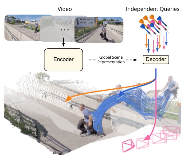
Figure 1: D4RT is a unified, efficient, feedforward method for Dynamic 4D Reconstruction and Tracking, unlocking a variety of outputs including point cloud (), point tracks (), camera parameters () through a single interface.
图 1:D4RT 是一种统一、高效的前馈方法,用于动态 4 维重建与跟**踪(Dynamic 4D Reconstruction and Tracking),通过单一接口即可得到点云、点轨迹、相机参数等多种输出。
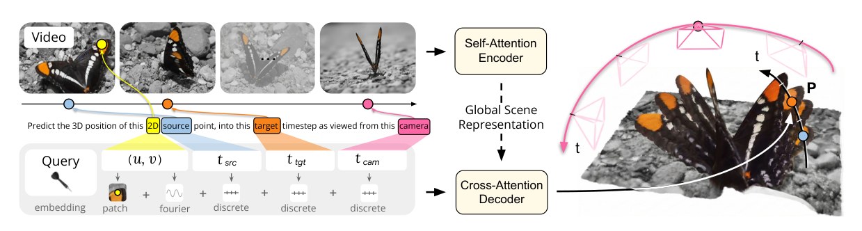
Figure 2: D4RT model overview – A global self-attention encoder first transforms the input video into the latent Global Scene Representation , which is passed to a lightweight decoder. The decoder can be independently queried for the 3D position of any given 2D point (, ) from the source timestep at target timestep in camera coordinate , unlocking full decoding at any point in space and time. The query also contains an embedding of the local video patch centered around (, ), providing additional spatial context.
图 2:D4RT 模型概览——全局自注意力编码器首先把输入视频变换为潜在的全局场景表示 ,再交给一个轻量解码器。解码器可被独立查询:给定源时刻 的二维点 ,即可得到其在目标时刻 、相机坐标系 下的三维位置 ,从而在任意时空点完成完整解码。查询中还包含以 为中心的局部视频图块嵌入,以提供额外的空间上下文。
We propose shifting the paradigm from fragmented, frame-level decoding to efficient, on-demand querying. We introduce D4RT, a feedforward method leveraging a flexible and scalable architecture to achieve full 4D reconstruction. As shown in Fig. 1, our model first encodes the input video, generating a latent scene representation which is then used to independently decode any number of spatio-temporal point queries. This simple, novel design unifies all 4D reconstruction tasks into a single interface and unlocks efficient training and inference.
我们主张把范式从碎片化的按帧解码,转向高效的按需查询。我们提出 D4RT,一种利用灵活、可扩展架构实现完整四维重建的前馈方法。如图 1 所示,模型先对输入视频编码,生成潜在场景表示,再据此独立解码任意数量的时空点查询。这一简洁的新设计把所有四维重建任务统一到单一接口,并解锁了高效的训练与推理。
Our key contributions are as follows:
本文的主要贡献如下:
- • We propose D4RT, a novel method for efficient feedforward querying of point-level 4D scene information captured in a video.
- 我们提出 D4RT,一种对视频中捕获的点级四维场景信息做高效前馈查询的新方法。
- • We demonstrate how our unified approach unlocks 4D correspondence, point clouds, depth maps, and camera parameters for both static and dynamic scenes through a single interface.
- 我们展示这一统一方法如何通过单一接口,为静态和动态场景同时给出四维对应、点云、深度图和相机参数。
- • In an extensive set of experiments, we show that D4RT sets a new state of the art in Dynamic 4D Reconstruction and Tracking while outperforming existing approaches in both speed and accuracy.
- 在大量实验中,我们表明 D4RT 在动态四维重建与跟踪上达到新的先进水平,并在速度和精度上同时超过已有方法。
- • Finally, we demonstrate how our flexible decoder unlocks an efficient algorithm to track all pixels in a video, enabling dense, holistic scene reconstruction.
- 最后,我们展示灵活的解码器如何支撑一种高效算法,以跟踪视频中的所有像素,从而实现稠密、整体的场景重建。
2 Method
2 方法
D4RT is based on a simple encoder-decoder architecture inspired by the Scene Representation Transformer [39, 40]. As shown in Fig. 2, the video is first processed by a powerful encoder producing the Global Scene Representation . The role of the encoder is to capture information about the full environment, identifying dense correspondence across all video frames, as well as understanding the flow of time and its effect on the scene. In a second stage, a lightweight decoder queries through a simple low-level interface. Specifically, given a 2D point in a source frame, the decoder predicts the 3D position of the point at a given target timestep (defining the temporal state) and expressed relative to a given camera reference (defined by the frame timestep where the camera viewpoint corresponds to this reference).
D4RT 基于受场景表示 Transformer(Scene Representation Transformer)[39, 40] 启发的简洁编码器–解码器架构。如图 2 所示,视频首先由强大的编码器处理,得到全局场景表示 。编码器的职责是捕获整个环境的信息,在所有视频帧之间识别稠密对应,并理解时间流及其对场景的影响。第二阶段,一个轻量解码器通过简单的底层接口查询 。具体而言,给定源帧中的一个二维点,解码器预测该点在给定目标时刻(定义时间状态)的三维位置,并相对于给定的相机参考(由与该参考相对应的帧时刻定义)来表示。
We draw attention to three desirable properties of this formulation: first, the indices need not coincide, allowing a full disentanglement of space and time; second, each query is decoded independently, allowing for both efficient training and inference as well as flexible decoding (both sparse and dense); and third, this interface unlocks a suite of downstream applications in a unified, consistent manner (Tab. 1).
这一表述有三个值得强调的性质:第一,各下标不必相同,从而可以把空间与时间完全拆开;第二,每个查询被独立解码,因而训练和推理都高效,解码也可以灵活地做稀疏或稠密;第三,这一接口以统一、一致的方式解锁了一系列下游应用(表 1)。
2.1 D4RT Framework
2.1 D4RT 框架
Given a video , the encoder extracts the latent Global Scene Representation
给定视频 ,编码器 提取潜在的全局场景表示
Once is calculated, it remains fixed throughout the second stage, where the decoder cross-attends from any number of queries into . We define a query , where correspond to source parameters and correspond to target parameters. Here, represent the normalized 2D coordinates of a point of interest in the source frame , while denote the temporal indices of the target timestep and the reference camera coordinate system (illustrated in Fig. 2). Each query is processed fully independently with the video features to produce its corresponding 3D point position :
一旦算出 ,它在第二阶段保持固定,解码器 从任意数量的查询出发对 做交叉注意力。我们定义查询 ,其中 对应源参数, 对应目标参数。这里, 表示源帧 中感兴趣点的归一化二维坐标,而 分别表示目标时刻与参考相机坐标系的时间下标(见图 2)。每个查询 都与视频特征 完全独立地处理,以产生对应的三维点位置 :
From query to 4D reconstruction. Through a simple variation of queries, our framework allows us to address a broad range of 4D tasks as shown in Tab. 1. Choosing any fixed point from a source frame in the video while varying produces its point track, the 3D trajectory of the corresponding point throughout the video. For full point cloud reconstruction, the 3D position of all pixels in the video can be directly predicted in a shared reference frame by the model. This alleviates the need for coordinate transformations to map pixels from different video frames into a unified coordinate system using explicit, potentially noisy camera estimates. Depth maps can be recovered by simply querying any pixel in the video with and only keeping the Z-dimension of the output .
从查询到四维重建。 只需对查询做简单变化,我们的框架就能覆盖表 1 所示的广泛四维任务。从视频源帧 中取定任意一点 ,同时令 变化,即可得到它的点轨迹,也就是该点在整段视频中的三维轨迹。若要做完整的点云重建,模型可以直接在共享参考系 下预测视频中所有像素的三维位置。这样就不必再用可能带噪的显式相机估计,把不同帧的像素变换到统一坐标系。深度图则只需对视频中任意像素取 做查询,并只保留输出 的 维即可恢复。
We next detail how camera extrinsics and intrinsics predictions are obtained. To derive the relative camera pose between any pair of video frames , we create queries for an ensemble of source points sampled on a grid in both reference frames:
接下来说明如何得到相机外参和内参预测。要推导任意一对视频帧 之间的相对相机位姿,我们在两帧参考下,对 网格上采样的一组源点 构造查询:
The resulting sets and describe the same 3D points in different reference frames. We therefore only need to find the rigid transformation between them, which can be efficiently derived through Umeyama’s algorithm [46] that solves a SVD decomposition.
得到的集合 与 描述的是同一组三维点在不同参考系下的坐标。因此只需找出它们之间的刚体变换,这可以通过 Umeyama 算法 [46] 高效完成,该方法求解一个 的 SVD 分解。
To recover intrinsics for video frame , we construct a set of queries for different source points, again sampled on a grid. We decode all corresponding 3D positions . Assuming a pinhole camera model with a principal point at , we get focal length parameters as follows:
要恢复视频帧 的内参,我们同样在 网格上为不同源点构造一组查询,解码出所有对应的三维位置 。假定针孔相机模型、主点在 ,焦距参数如下:
We take the median over the estimates for robustness. Camera models with distortion (e.g., fisheye) can also be seamlessly incorporated by adding a non-linear refinement step on top of the initial estimation [61].
为提高稳健性,我们对这 个估计取中位数。带畸变的相机模型(例如鱼眼)也可以无缝纳入:只需在初始估计之上再加一步非线性精修 [61]。
| Task | Query | |||
|---|---|---|---|---|
| Point Track | Fixed | Fixed | Fixed | … |
| Point Cloud | … | … | … | Fixed |
| Depth Map | … | … | … | |
| Extrinsics | Fixed | … | ||
| Intrinsics | … |
Table 1: Unified decoding – A diverse set of geometry-related tasks can be inferred by querying the Cartesian product of the respective entries. Note that for intrinsics and extrinsics, we only query a coarse grid for faster inference.
| 任务 | 查询 | |||
|---|---|---|---|---|
| 点轨迹 | 固定 | 固定 | 固定 | … |
| 点云 | … | … | … | 固定 |
| 深度图 | … | … | … | |
| 外参 | 固定 | … | ||
| 内参 | … |
表 1:统一解码——通过对相应条目做笛卡尔积查询,可以推断出多种与几何相关的任务。注意,对于内参和外参,我们只在较粗的 网格上查询,以加快推理。
2.2 Model Architecture
2.2 模型架构
Our encoder is based on the Vision Transformer [9] with interleaved local frame-wise, and global self-attention layers [48]. For simplicity, and to support arbitrary aspect ratios, we resize the input video to a fixed square resolution before tokenizing it. To incorporate the original aspect ratio, we embed it into a separate token and pass it to the transformer along with the main video tokens.
编码器 基于视觉 Transformer [9],并交错使用局部按帧自注意力与全局自注意力层 [48]。为简单起见,同时支持任意长宽比,我们在分词前把输入视频缩放为固定的方形分辨率。为纳入原始长宽比,我们把它嵌入一个单独的 token,并与主视频 token 一并送入 Transformer。
Pointwise decoder. The decoder is a small cross-attention transformer. A query token is first constructed by adding the Fourier feature embedding [47] of the 2D coordinates to the learned discrete timestep embeddings for , , and . We empirically observe that augmenting the query with an embedding of the local pixel RGB patch centered at dramatically improves performance, see Sec. 4.4.
逐点解码器。 解码器 是一个小型交叉注意力 Transformer。查询 token 首先由二维坐标 的傅里叶特征嵌入 [47],与 、 和 的可学习离散时刻嵌入相加构成。我们经验上观察到,再为查询附上以 为中心的局部 像素 RGB 图块嵌入,会显著提升性能,见第 4.4 节。
Each query is decoded independently through cross-attention into the Global Scene Representation , ensuring that queries do not interact. The resulting output feature is then mapped to a 3D point position via a simple learned projection. Decoding queries independently is a deliberate design decision with major advantages. It allows efficient training, as only a small number of queries need to be decoded to provide a supervision signal to the model. Equally importantly, at inference time, the queries can be chosen freely across all video frames as described in Sec. 2.3, and need not be correlated to each other to avoid out-of-distribution effects – indeed, we have empirically observed major performance drops when enabling self-attention between queries in early experiments. Finally, this design allows highly efficient inference thanks to its trivial parallelism. As shown in Fig. 3 and Tab. 3, we obtain the best trade-off between performance and latency across multiple tasks.
每个查询都通过交叉注意力独立解码到全局场景表示 中,从而保证查询之间互不交互。得到的输出特征再经一个简单的可学习投影映射为三维点位置 。让查询独立解码是有意为之的设计,好处很大。它使训练更高效,因为只需解码少量查询就能为模型提供监督信号。同样重要的是,推理时可以按第 2.3 节所述,在全部视频帧上自由选择查询,查询之间不必相关,以免出现分布外效应——事实上,早期实验中若在查询之间启用自注意力,我们观察到性能会大幅下降。最后,这一设计因近乎平凡的并行性而能实现非常高效的推理。如图 3 和表 3 所示,我们在多项任务上取得了性能与延迟之间的最佳权衡。
1: Input video , model encoder and decoder .
2: Compute Global Scene Representation
3: Initialize Occupancy Grid
4: Initialize Set of Dense Tracks
5: while any() do
6: Sample a batch of unvisited source points from
7: for each do Process batch in parallel
8: Get Track Queries
9: Run the decoder
10: Set visible track pixels as visited
11: Add new track to the output
12: end for
13: end while
14: return
Algorithm 1 Efficient Dense Tracking of All Pixels.
1: 输入视频 ,模型编码器 与解码器 。
2: 计算全局场景表示
3: 初始化占用网格
4: 初始化稠密轨迹集合
5: while any() do
6: 从 中采样一批未访问的源点
7: for 每个 do 批量并行处理
8: 得到轨迹查询
9: 运行解码器
10: 将轨迹上可见的像素标为已访问
11: 把新轨迹加入输出
12: end for
13: end while
14: return
算法 1 高效地密集跟踪所有像素。
2.3 Training and Inference
2.3 训练与推理
The model is implemented in Kauldron [15] and trained end-to-end by minimizing the weighted sum of losses computed over a batch of sampled queries. The primary supervision signal is derived from an loss applied to the normalized 3D point position . Specifically, both the target and the estimated point sets are normalized by their respective mean depths [51] and then passed through the transform to dampen the influence of far-away points on the loss. We also supervise a set of auxiliary predictions from additional linear projections on the decoder output: An loss on 2D coordinates of the point positions in image space; cosine similarity for 3D surface normals [54]; binary cross-entropy for target point visibility; and on the vector of point motion. All loss terms are applied only where ground truth supervision is available. We finally incorporate a confidence penalty where additionally weights the 3D point error [25].
模型在 Kauldron [15] 中实现,通过最小化在一批 个采样查询上计算的加权损失之和来端到端训练。主要监督信号来自作用于归一化三维点位置 的 损失。具体而言,目标点集与估计点集都先按各自的平均深度归一化 [51],再经过变换 ,以减弱远处点对损失的影响。我们还从解码器输出上额外的线性投影得到一组辅助预测并加以监督:对图像空间中点位置的二维坐标用 损失;对三维表面法向用余弦相似度 [54];对目标点可见性用二元交叉熵;对点运动向量用 。所有损失项仅在有真值监督的位置上施加。最后我们加入置信度惩罚 ,其中 还会对三维点误差加权 [25]。
Efficient dense dynamic correspondence. A key capability of our query-based model is that it can efficiently compute dense correspondences for all pixels in a video, both static and dynamic. As shown in Fig. 4, this capability is crucial for building a complete, holistic scene reconstruction, which in turn is key to eliminating the occlusion-induced discontinuities and sparse artifacts common in prior works. However, a naive approach to reconstruct tracks for all pixels across the video would involve queries, the majority of which are not required.
高效的稠密动态对应。 基于查询的模型有一项关键能力:它能高效地为视频中所有像素计算稠密对应,无论静态还是动态。如图 4 所示,这一能力对于构建完整、整体的场景重建至关重要,而完整重建又是消除先前工作中常见的、由遮挡引起的间断和稀疏伪影的关键。然而,若朴素地为视频中所有像素重建轨迹,将涉及 次查询,其中绝大多数并非必需。
We introduce Alg. 1 which exploits spatio-temporal redundancy using an occupancy grid to speed this procedure up significantly. The algorithm only initiates new tracks from unvisited pixels. Each full-video track marks all spatio-temporal pixels it visibly passes through as visited. Empirically, we find that this yields an adaptive speedup between 5–15 depending on the motion complexity in the video. This dense, flexible strategy is feasible for our method precisely because our decoder is both sparse, and lightweight. It is notable that prior works are ill-suited for this task for various reasons. Most methods fail to provide any correspondences for dynamic portions of the scenes [48, 54, 29], dense frame-level decoding remains locked in the costly naive approach [11], and models with heavy sparse decoders face a large per-query cost [23, 56].
我们提出算法 1,利用占用网格 挖掘时空冗余,从而显著加速这一过程。算法只从未访问像素发起新轨迹。每条整段视频轨迹会把它可见地经过的所有时空像素标记为已访问。经验上,这一做法会带来随视频运动复杂度而变化的 5–15 倍自适应加速。这种稠密而灵活的策略之所以可行,正是因为我们的解码器既稀疏又轻量。值得注意的是,已有工作因种种原因并不适合这一任务:多数方法无法为场景的动态部分提供任何对应 [48, 54, 29];稠密的按帧解码仍困在代价高昂的朴素做法里 [11];而带有沉重稀疏解码器的模型则面临很高的单查询成本 [23, 56]。
| Model | Task | Functionality | Architecture | |||
|---|---|---|---|---|---|---|
| 3D Recon- | Dynamic Cor- | Flexible | Sparse | Global | Single | |
| struction | respondence | Ref. Frames | Decoding | Context | Decoder | |
| MegaSaM [29] | ✓ | ✗ | ✗ | ✗ | ✗ | ✗ |
| DUSt3R[51] | ✓ | ✗ | ✗ | ✗ | ✗ | ✗ |
| VGGT [48] | ✓ | ✗ | ✗ | ✗ | ✓ | ✗ |
| [54] | ✓ | ✗ | ✓ | ✗ | ✓ | ✗ |
| St4RTrack [11] | ✓ | ✓ | ✗ | ✗ | ✗ | ✗ |
| STv2 [56] | ✓ | ✓ | ✗ | ✓ | ✓ | ✗ |
| D4RT (Ours) | ✓ | ✓ | ✓ | ✓ | ✓ | ✓ |
Table 2: Model capabilities – We highlight both the tasks our model executes but also its comprehensive functionality and simple model architecture.
| 模型 | 任务 | 功能 | 架构 | |||
|---|---|---|---|---|---|---|
| 三维重 | 动态对 | 灵活的 | 稀疏 | 全局 | 单一 | |
| 建 | 应关系 | 参考帧 | 解码 | 上下文 | 解码器 | |
| MegaSaM [29] | ✓ | ✗ | ✗ | ✗ | ✗ | ✗ |
| DUSt3R[51] | ✓ | ✗ | ✗ | ✗ | ✗ | ✗ |
| VGGT [48] | ✓ | ✗ | ✗ | ✗ | ✗ | ✗ |
| [54] | ✓ | ✗ | ✓ | ✗ | ✓ | ✗ |
| St4RTrack [11] | ✓ | ✓ | ✗ | ✗ | ✗ | ✗ |
| STv2 [56] | ✓ | ✓ | ✗ | ✓ | ✓ | ✗ |
| D4RT(本文) | ✓ | ✓ | ✓ | ✓ | ✓ | ✓ |
表 2:模型能力——我们既突出模型所执行的任务,也强调其全面的功能与简洁的模型架构。
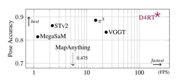
Figure 3: Pose accuracy vs. speed – We compare pose accuracy vs. throughput against recent state-of-the-art methods. Pose accuracy is 1 – error, averaged over ATE/RTE/RPE on Sintel and ScanNet. Throughput is measured in FPS on an A100 GPU. D4RT achieves 200+ FPS pose estimation, 9 faster than VGGT, and 100 faster than MegaSaM, while delivering superior accuracy.
图 3:位姿精度与速度——我们将位姿精度与吞吐和近期先进方法做比较。位姿精度定义为 1 − 误差,在 Sintel 与 ScanNet 上对 ATE/RTE/RPE 取平均。吞吐以一块 A100 GPU 上的 FPS 衡量。D4RT 的位姿估计达到 200+ FPS,大约比 VGGT 快 9 倍,比 MegaSaM 快 100 倍,同时精度更高。
3 Related Work
3 相关工作
Classical approaches to 3D reconstruction are fundamentally anchored in multi-view geometry, specifically Structure-from-Motion (SfM) [19, 33] and Multi-View Stereo (MVS) [12, 43]. The standard pipeline exemplified by COLMAP [42] incrementally estimates and optimizes sparse geometry and camera poses. The advantage of these methods is their explicit enforcement of geometric consistency and mathematically interpretable reconstructions. However, they are computationally intensive and brittle.
经典的三维重建方法从根本上锚定于多视图几何,尤其是运动恢复结构(Structure-from-Motion, SfM)[19, 33] 与多视图立体(Multi-View Stereo, MVS)[12, 43]。以 COLMAP [42] 为代表的标准流程,增量式地估计并优化稀疏几何与相机位姿。这类方法的优点是显式强制几何一致性,重建结果在数学上也可解释。但它们计算密集,而且比较脆弱。
3.1 Feedforward 3D Reconstruction
3.1 前馈三维重建
The field of 3D reconstruction has recently shifted towards end-to-end, feedforward models that directly infer geometry from images. The seminal work DUSt3R [51] demonstrated that Transformer-based networks [47] can perform 3D reconstruction from unposed and uncalibrated image pairs in an end-to-end approach. VGGT [48] later scaled this approach beyond pairs by using a Vision Transformer [9] with global attention. Building on this feedforward paradigm, several works have extended the methodology to dynamic videos [60, 50, 52, 3] and more efficient inference [54, 57]. However, these models share significant limitations. For instance, many do not support changing camera intrinsics within a video [54, 48, 29], and several are restricted to using only the first frame as the camera reference [51, 29, 50]. More importantly, architectures inspired by VGGT [48] either use separate decoder heads for each task [60, 50, 54] (e.g., depth, pose, point cloud), or they incorporate separate models for sub-tasks of 4D reconstruction [52, 31, 44], making the full pipeline cumbersome and computationally expensive to run. Finally, these methods are not directly capable of providing correspondences for dynamic regions of the scene.
三维重建领域近来转向端到端、前馈的模型,直接从图像推断几何。开创性工作 DUSt3R [51] 表明,基于 Transformer 的网络 [47] 能够以端到端方式,从未位姿、未标定的图像对进行三维重建。VGGT [48] 随后用带全局注意力的视觉 Transformer [9],把这一做法扩展到图像对之外。沿着这一前馈范式,已有工作把方法推广到动态视频 [60, 50, 52, 3] 以及更高效的推理 [54, 57]。不过,这些模型有一些共同的明显局限。例如,许多方法不支持在同一段视频中改变相机内参 [54, 48, 29],还有一些只能把第一帧当作相机参考 [51, 29, 50]。更重要的是,受 VGGT [48] 启发的架构要么为每个任务使用单独的解码头 [60, 50, 54](例如深度、位姿、点云),要么为四维重建的子任务引入单独模型 [52, 31, 44],使整条流水线既臃肿又昂贵。最后,这些方法并不能直接为场景的动态区域提供对应关系。
| Input video | MegaSaM [29] | [54] | SpatialTrackerV2 [56] | D4RT (Ours) |
|---|
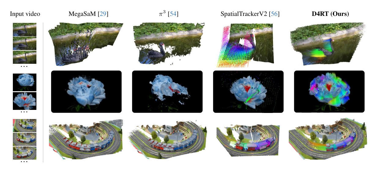
Figure 4: Reconstruction results across methods – Pure reconstruction methods (MegaSaM and ) are only able to accumulate point clouds of all pixels; exhibiting clear failure cases in dynamic scenes. For example, the swan is repeated in MegaSaM’s reconstruction, and is failing entirely to reconstruct the flower. SpatialTrackerV2, a state-of-the-art tracking method, successfully captures dynamics, however its design only allows tracking points from one frame, leaving gaps in the reconstruction (behind the swan and train). D4RT is the only method that successfully reconstructs a full 4D representation of the scene including all pixels of the video.
| 输入视频 | MegaSaM [29] | [54] | SpatialTrackerV2 [56] | D4RT(本文) |
|---|
图 4:各方法的重建结果——纯重建方法(MegaSaM 与 )只能把所有像素的点云累加起来,在动态场景中出现明显失败:例如 MegaSaM 的重建里天鹅被重复,而 完全没能重建出花朵。先进的跟踪方法 SpatialTrackerV2 能够抓住动态,但其设计只允许从一帧跟踪点,重建中会留下空隙(天鹅与列车后方)。D4RT 是唯一成功重建出完整四维场景表示、并覆盖视频中所有像素的方法。
3.2 From 2D to 3D Point Tracking
3.2 从二维点跟踪到三维点跟踪
The task of point tracking aims to establish long-term 2D correspondences through challenges like occlusions and non-rigid motion, evolving from early methods such as Particle Video [41] to newer deep-learning approaches [17, 7, 8, 63]. This field has further progressed from tracking a sparse set of points to the dense tracking of every pixel in a video [28, 32, 18]. A parallel line of work has explored lifting these 2D tracks into 3D, which is achieved by projecting tracks from image space to camera coordinates using ground truth or predicted depth and camera intrinsics [27].
点跟踪的任务是在遮挡和非刚性运动等困难下建立长期二维对应,从早期的 Particle Video [41] 发展到较新的深度学习方法 [17, 7, 8, 63]。这一领域进一步从跟踪稀疏点集,走到对视频中每个像素做稠密跟踪 [28, 32, 18]。另一条并行线索则探索把这些二维轨迹提升到三维,做法是利用真值或预测的深度与相机内参,把轨迹从图像空间投影到相机坐标 [27]。
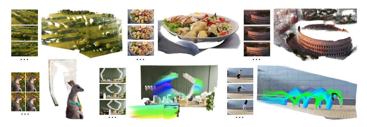
Figure 5: Visualizations on in-the-wild videos – D4RT demonstrates accurate reconstructions on static (top row) and dynamic scenes (bottom row). In the presence of motion, D4RT additionally produces robust 3D point trajectories.
图 5:野外视频上的可视化——D4RT 在静态(上行)和动态场景(下行)上都给出准确的重建。在存在运动时,D4RT 还能给出稳健的三维点轨迹。
Most recently, models like SpatialTracker [55, 56], L4P [1], DPM [44] and St4RTracker [11] have moved to directly predicting 3D tracks without priors. Yet, limitations remain: St4RTracker [11] and DPM [44] follow the pairwise paradigm of DUSt3R [51], preventing holistic video processing. SpatialTrackerV2 [56] is a multi-stage approach and exhibits slow inference speeds as it relies on iterative refinements. Meanwhile, L4P [1] requires different heads for sparse and dense outputs of the same nature (e.g., flow vs. 2D tracking or depth vs. 3D tracking). In contrast, our approach unifies these tasks within a single architecture. Tab. 2 summarizes capabilities across a recent set of state-of-the-art models.
最近,SpatialTracker [55, 56]、L4P [1]、DPM [44] 和 St4RTracker [11] 等模型转向在不依赖先验的情况下直接预测三维轨迹。局限仍然存在:St4RTracker [11] 与 DPM [44] 沿用 DUSt3R [51] 的成对范式,无法对整段视频做整体处理。SpatialTrackerV2 [56] 是多阶段方法,依赖迭代精修,推理速度较慢。而 L4P [1] 对同一类输出的稀疏与稠密形式需要不同的头(例如光流对二维跟踪,或深度对三维跟踪)。相比之下,我们的方法在单一架构内统一了这些任务。表 2 汇总了近期一批先进模型的能力。
4 Experiments
4 实验
We benchmark D4RT against recent state-of-the-art methods. After inspecting qualitative differences in capability in Sec. 4.1, we proceed with evaluating 4D Reconstruction and Tracking performance in Sec. 4.2, focusing the comparison on the best methods from Sec. 3.2. We then continue with pure reconstruction tasks in Sec. 4.3, comparing to the recent SOTA models mentioned in Sec. 3.1. We conclude with a set of key ablations in Sec. 4.4.
我们将 D4RT 与近期先进方法做基准比较。在第 4.1 节检视能力上的定性差异之后,第 4.2 节评估四维重建与跟踪性能,比较对象集中在第 3.2 节中表现最好的方法。随后第 4.3 节继续讨论纯重建任务,与第 3.1 节提到的近期先进模型比较。最后在第 4.4 节给出一组关键消融。
Training setup. For the encoder, we use the ViT-g model variant with 40 layers on a spatio-temporal patch size of . This encoder and our 8-layer cross-attention decoder contain 1 B and 144 M parameters, respectively. Our training mixture contains public and internal datasets including BlendedMVS [58], Co3Dv2 [38], Dynamic Replica [22], Kubric [16], MVS-Synth [20], PointOdyssey [62], ScanNet++ [59], ScanNet [4], Tartanair [53], VirtualKitti [13], and Waymo Open [45]. We train on 48-frame clips at resolution, decoding 2048 random queries that are oversampled on specific regions for more efficient training , see the appendix for details. The model is trained for 500 k steps using the AdamW optimizer [26, 30] with a local batch size of 1 across 64 TPU chips, taking a total of just over 2 days to complete.
训练设置。 编码器采用 ViT-g 变体,共 40 层,时空图块大小为 。该编码器与我们 8 层的交叉注意力解码器分别含有 10 亿和 1.44 亿参数。训练混合包含公开与内部数据集,包括 BlendedMVS [58]、Co3Dv2 [38]、Dynamic Replica [22]、Kubric [16]、MVS-Synth [20]、PointOdyssey [62]、ScanNet++ [59]、ScanNet [4]、Tartanair [53]、VirtualKitti [13] 以及 Waymo Open [45]。我们在 分辨率的 48 帧片段上训练,解码 2048 个随机查询,并在特定区域过采样以提高训练效率,细节见附录。模型用 AdamW 优化器 [26, 30] 训练 50 万步,在 64 块 TPU 上本地批量大小为 1,总共只需略多于两天即可完成。
| Method | Max. Track Count @ Target FPS | |||
|---|---|---|---|---|
| 60 FPS | 24 FPS | 10 FPS | 1 FPS | |
| DELTA [32] | 0 | 5 | 408 | 5,770 |
| SpatialTrackerV2 [56] | 29 | 84 | 219 | 2,290 |
| D4RT (Ours) | 550 | 1,570 | 3,890 | 40,180 |
Table 3: 3D tracking throughput – We measure the maximum number of full-video 3D point tracks that different model can produce while maintaining a given FPS target on a single A100 GPU. Note that for D4RT, each track consists of independent queries processed by the decoder. D4RT is 18–300 faster than others.
| 方法 | 给定目标 FPS 下的最大轨迹数 | |||
|---|---|---|---|---|
| 60 FPS | 24 FPS | 10 FPS | 1 FPS | |
| DELTA [32] | 0 | 5 | 408 | 5,770 |
| SpatialTrackerV2 [56] | 29 | 84 | 219 | 2,290 |
| D4RT(本文) | 550 | 1,570 | 3,890 | 40,180 |
表 3:三维跟踪吞吐——我们测量不同模型在单块 A100 GPU 上、维持给定 FPS 目标时,最多能产生多少条整段视频的三维点轨迹。注意,对 D4RT 而言,每条轨迹由解码器处理的 个独立查询组成。D4RT 比其他方法快 18–300 倍。
| w/ GT intrin. | Method | TAPVid-3D | ||||||||||||
|---|---|---|---|---|---|---|---|---|---|---|---|---|---|---|
| Camera Coordinate 3D tracking | World Coordinate 3D tracking | |||||||||||||
| DriveTrack | ADT | PStudio | DriveTrack | ADT | ||||||||||
| AJ | OA | AJ | OA | AJ | OA | L1 | L1 | |||||||
| ✗ | St4RTrack [11] | - | - | - | - | - | - | - | - | - | 0.020 | 0.499 | 0.062 | 0.839 |
| CoTracker3 [23] + UniDepthV2 [36] | 0.038 | 0.062 | 0.856 | 0.102 | 0.146 | 0.937 | 0.119 | 0.176 | 0.862 | - | - | - | - | |
| CoTracker3 [23] + VGGT [48] | 0.129 | 0.189 | 0.856 | 0.132 | 0.190 | 0.937 | 0.045 | 0.070 | 0.862 | 0.205 | 0.170 | 0.192 | 0.736 | |
| SpatialTrackerV2 [56] | 0.064 | 0.100 | 0.865 | 0.260 | 0.342 | 0.936 | 0.097 | 0.152 | 0.805 | 0.101 | 0.139 | 0.336 | 0.238 | |
| D4RT (Ours) | 0.257 | 0.345 | 0.875 | 0.240 | 0.319 | 0.926 | 0.138 | 0.186 | 0.897 | 0.373 | 0.020 | 0.319 | 0.096 | |
| ✓ | CoTracker3 [23] + UniDepthV2 [36] | 0.147 | 0.225 | 0.856 | 0.173 | 0.254 | 0.937 | 0.205 | 0.311 | 0.862 | - | - | - | - |
| CoTracker3 [23] + VGGT [48] | 0.245 | 0.342 | 0.856 | 0.175 | 0.250 | 0.937 | 0.215 | 0.318 | 0.862 | 0.292 | 0.160 | 0.234 | 0.755 | |
| DELTA [32] | 0.170 | 0.238 | 0.874 | 0.199 | 0.258 | 0.879 | 0.175 | 0.261 | 0.760 | - | - | - | - | |
| SpatialTrackerV2 [56] | 0.195 | 0.275 | 0.865 | 0.303 | 0.404 | 0.936 | 0.175 | 0.270 | 0.805 | 0.201 | 0.117 | 0.378 | 0.263 | |
| D4RT (Ours) | 0.304 | 0.410 | 0.875 | 0.307 | 0.408 | 0.926 | 0.372 | 0.498 | 0.897 | 0.470 | 0.017 | 0.398 | 0.093 |
Table 4: 4D reconstruction and tracking – We evaluate 3D tracking capability on dynamic videos, with tracks predicted in both local camera coordinates (left) and world coordinates (right). Our model achieves superior performance compared to the prior state-of-the-art.
| 使用真值内参 | 方法 | TAPVid-3D | ||||||||||||
|---|---|---|---|---|---|---|---|---|---|---|---|---|---|---|
| 相机坐标三维跟踪 | 世界坐标三维跟踪 | |||||||||||||
| DriveTrack | ADT | PStudio | DriveTrack | ADT | ||||||||||
| AJ | OA | AJ | OA | AJ | OA | L1 | L1 | |||||||
| ✗ | St4RTrack [11] | - | - | - | - | - | - | - | - | - | 0.020 | 0.499 | 0.062 | 0.839 |
| CoTracker3 [23] + UniDepthV2 [36] | 0.038 | 0.062 | 0.856 | 0.102 | 0.146 | 0.937 | 0.119 | 0.176 | 0.862 | - | - | - | - | |
| CoTracker3 [23] + VGGT [48] | 0.129 | 0.189 | 0.856 | 0.132 | 0.190 | 0.937 | 0.045 | 0.070 | 0.862 | 0.205 | 0.170 | 0.192 | 0.736 | |
| SpatialTrackerV2 [56] | 0.064 | 0.100 | 0.865 | 0.260 | 0.342 | 0.936 | 0.097 | 0.152 | 0.805 | 0.101 | 0.139 | 0.336 | 0.238 | |
| D4RT(本文) | 0.257 | 0.345 | 0.875 | 0.240 | 0.319 | 0.926 | 0.138 | 0.186 | 0.897 | 0.373 | 0.020 | 0.319 | 0.096 | |
| ✓ | CoTracker3 [23] + UniDepthV2 [36] | 0.147 | 0.225 | 0.856 | 0.173 | 0.254 | 0.937 | 0.205 | 0.311 | 0.862 | - | - | - | - |
| CoTracker3 [23] + VGGT [48] | 0.245 | 0.342 | 0.856 | 0.175 | 0.250 | 0.937 | 0.215 | 0.318 | 0.862 | 0.292 | 0.160 | 0.234 | 0.755 | |
| DELTA [32] | 0.170 | 0.238 | 0.874 | 0.199 | 0.258 | 0.879 | 0.175 | 0.261 | 0.760 | - | - | - | - | |
| SpatialTrackerV2 [56] | 0.195 | 0.275 | 0.865 | 0.303 | 0.404 | 0.936 | 0.175 | 0.270 | 0.805 | 0.201 | 0.117 | 0.378 | 0.263 | |
| D4RT(本文) | 0.304 | 0.410 | 0.875 | 0.307 | 0.408 | 0.926 | 0.372 | 0.498 | 0.897 | 0.470 | 0.017 | 0.398 | 0.093 |
表 4:四维重建与跟踪——我们在动态视频上评估三维跟踪能力,轨迹分别在局部相机坐标(左)和世界坐标(右)中预测。我们的模型优于此前的先进水平。
4.1 Qualitative Analysis
4.1 定性分析
We begin our evaluations by inspecting video reconstruction quality in Fig. 4. Dynamic objects (e.g., swan and train) reveal qualitative differences, highlighting performance gaps between different methods. Pure reconstruction methods (see Sec. 3.1), exemplified by the state-of-the-art models MegaSaM and , fail to understand dynamics in the scenes, producing either repeated images of the entities as they move through the scene, or failing to reconstruct them altogether. Conversely, tracking-based models successfully reconstruct and track dynamics. However, they commonly only track points from one frame, leaving gaps in the reconstruction in all areas that are occluded in the first frame as seen for SpatialTrackerV2 [56] here. Meanwhile, D4RT is able to track all dynamic pixels of the video in a unified reference frame. We further evaluate our method on diverse in-the-wild videos in Fig. 5, demonstrating its performance to both static and dynamic scenes.
我们首先在图 4 中检视视频重建质量。动态物体(例如天鹅和列车)揭示了各方法之间的定性差异,也凸显了性能差距。纯重建方法(见第 3.1 节),以先进模型 MegaSaM 和 为例,未能理解场景中的动态,要么把实体在运动过程中重复成像,要么完全没能重建出来。与此相对,基于跟踪的模型能够重建并跟踪动态。不过它们通常只从一帧跟踪点,凡是在第一帧被遮挡的区域,重建中都会留下空隙,如此处的 SpatialTrackerV2 [56] 所示。而 D4RT 能够在统一参考系下跟踪视频中的全部动态像素。我们还在图 5 中于多样的野外视频上评估本方法,展示它在静态和动态场景上的表现。
4.2 4D Reconstruction and Tracking
4.2 四维重建与跟踪
| Method | Point Cloud | Video Depth | ||||||||
|---|---|---|---|---|---|---|---|---|---|---|
| Sintel | Scannet | Sintel | ScanNet | KITTI | Bonn | |||||
| L1 | L1 | AbsRel (S) | AbsRel (SS) | AbsRel (S) | AbsRel (SS) | AbsRel (S) | AbsRel (SS) | AbsRel (S) | AbsRel (SS) | |
| MegaSaM [29] | 1.531 | 0.072 | 0.342 | 0.249 | 0.050 | 0.047 | 0.109 | 0.101 | 0.056 | 0.056 |
| VGGT [48] | 1.582 | 0.063 | 0.318 | 0.247 | 0.044 | 0.040 | 0.094 | 0.067 | 0.055 | 0.051 |
| MapAnything [24] | 1.718 | 0.064 | 0.397 | 0.306 | 0.043 | 0.035 | 0.096 | 0.090 | 0.076 | 0.049 |
| SpatialTrackerV2 [56] | 1.375 | 0.036 | 0.209 | 0.175 | 0.027 | 0.025 | 0.075 | 0.064 | 0.042 | 0.978 |
| [54] | 1.139 | 0.030 | 0.241 | 0.163 | 0.021 | 0.019 | 0.055 | 0.053 | 0.033 | 0.032 |
| D4RT (Ours) | 0.768 | 0.028 | 0.171 | 0.148 | 0.020 | 0.018 | 0.055 | 0.051 | 0.036 | 0.036 |
Table 5: Video depth and point map estimation – Quantitative results for both video depth and point map estimation across four benchmarks. D4RT achieves top-tier performance on the depth estimation task under both scale-only (S) and scale-and-shift (SS) alignments.
| 方法 | 点云 | 视频深度 | ||||||||
|---|---|---|---|---|---|---|---|---|---|---|
| Sintel | ScanNet | Sintel | ScanNet | KITTI | Bonn | |||||
| L1 | L1 | AbsRel (S) | AbsRel (SS) | AbsRel (S) | AbsRel (SS) | AbsRel (S) | AbsRel (SS) | AbsRel (S) | AbsRel (SS) | |
| MegaSaM [29] | 1.531 | 0.072 | 0.342 | 0.249 | 0.050 | 0.047 | 0.109 | 0.101 | 0.056 | 0.056 |
| VGGT [48] | 1.582 | 0.063 | 0.318 | 0.247 | 0.044 | 0.040 | 0.094 | 0.067 | 0.055 | 0.051 |
| MapAnything [24] | 1.718 | 0.064 | 0.397 | 0.306 | 0.043 | 0.035 | 0.096 | 0.090 | 0.076 | 0.049 |
| SpatialTrackerV2 [56] | 1.375 | 0.036 | 0.209 | 0.175 | 0.027 | 0.025 | 0.075 | 0.064 | 0.042 | 0.978 |
| [54] | 1.139 | 0.030 | 0.241 | 0.163 | 0.021 | 0.019 | 0.055 | 0.053 | 0.033 | 0.032 |
| D4RT(本文) | 0.768 | 0.028 | 0.171 | 0.148 | 0.020 | 0.018 | 0.055 | 0.051 | 0.036 | 0.036 |
表 5:视频深度与点图估计——四个基准上视频深度与点图估计的定量结果。在仅尺度(S)以及尺度加平移(SS)两种对齐下,D4RT 在深度估计任务上都达到第一梯队的表现。
We now turn to the quantitative evaluation of 4D Reconstruction and Tracking, comparing D4RT to other methods that can estimate dynamic correspondences. We evaluate on TAPVid-3D [27] which is comprised of three subsets of real-world videos in challenging settings.
接下来我们对四维重建与跟踪做定量评估,把 D4RT 与其他能够估计动态对应的方法相比较。评估在 TAPVid-3D [27] 上进行,该基准由三组具有挑战性设定的真实世界视频子集组成。
We first evaluate 3D tracking in the local camera frame using the standard protocol from Koppula et al. [27], which measures a model’s ability to predict and track the 3D position of every observed point in the local camera reference frames. We report standard 3D tracking metrics Average percent of points within delta error , Occlusion Accuracy (OA) and 3D Average Jaccard (AJ). As shown in Tab. 4 (left), D4RT achieves state-of-the-art results against competing methods, both with and without known ground-truth intrinsics.
我们首先按 Koppula 等人 [27] 的标准协议,在局部相机坐标系中评估三维跟踪,衡量模型在局部相机参考系下预测并跟踪每个被观测点三维位置的能力。我们报告标准的三维跟踪指标:误差在阈值内的点的平均百分比 、遮挡准确率(OA)以及三维平均 Jaccard(AJ)。如表 4(左)所示,无论是否已知真值内参,D4RT 都相对竞争方法取得了先进结果。
Tab. 4 (right) shows results for world coordinate 3D tracking. This task measures a model’s ability to predict tracks within a single, consistent world coordinate system, thereby also measuring the models’ ability to implicitly change reference frames. PStudio is omitted here as it has no camera motion, rendering this task effectively identical to the preceding one. Since there is no concept of occlusion for this task, we report as well as the L1 distance between the predicted and ground-truth tracks which provides a comprehensive, global measure of deviation. We observe that our model excels at this task as well, exhibiting strong improvements across metrics.
表 4(右)给出世界坐标三维跟踪的结果。该任务衡量模型在单一、一致的世界坐标系中预测轨迹的能力,因而也衡量模型隐式变换参考系的能力。此处省略 PStudio,因为它没有相机运动,这一任务实际上与前一项相同。由于该任务没有遮挡的概念,我们报告 以及预测轨迹与真值轨迹之间的 L1 距离,后者提供了对偏差的全面、全局度量。我们看到,本模型在这一任务上同样表现出色,各项指标都有明显提升。
We finally compare efficiency in Tab. 3, by counting the number of tracks each model can produce for a given target frame-per-second rate (FPS). The measurements show that our model is 18-300 faster than prior methods.
最后,我们在表 3 中比较效率,统计各模型在给定目标帧率(FPS)下能够产生的轨迹数量。测量表明,我们的模型比先前方法快 18–300 倍。
| Method | Sintel | ScanNet | Re10K | ||||
|---|---|---|---|---|---|---|---|
| ATE | RPE-T | RPE-R | ATE | RPE-T | RPE-R | Pose AUC | |
| MegaSaM [29] | 0.074 | 0.030 | 0.126 | 0.029 | 0.016 | 0.839 | 71.0 |
| VGGT [48] | 0.168 | 0.056 | 0.428 | 0.016 | 0.012 | 0.316 | 70.2 |
| MapAnything [24] | 0.202 | 0.089 | 2.383 | 0.023 | 0.016 | 0.438 | 68.7 |
| SpatialTrackerV2 [56] | 0.126 | 0.053 | 1.052 | 0.018 | 0.012 | 0.324 | 75.7 |
| [54] | 0.086 | 0.039 | 0.248 | 0.015 | 0.010 | 0.291 | 78.7 |
| D4RT (Ours) | 0.065 | 0.024 | 0.126 | 0.014 | 0.010 | 0.302 | 83.5 |
Table 6: Camera pose estimation – We evaluate D4RT against state-of-the-art methods on static indoor scenes (ScanNet, Re10K) and dynamic outdoor scenes (Sintel).
| 方法 | Sintel | ScanNet | Re10K | ||||
|---|---|---|---|---|---|---|---|
| ATE | RPE-T | RPE-R | ATE | RPE-T | RPE-R | 位姿 AUC | |
| MegaSaM [29] | 0.074 | 0.030 | 0.126 | 0.029 | 0.016 | 0.839 | 71.0 |
| VGGT [48] | 0.168 | 0.056 | 0.428 | 0.016 | 0.012 | 0.316 | 70.2 |
| MapAnything [24] | 0.202 | 0.089 | 2.383 | 0.023 | 0.016 | 0.438 | 68.7 |
| SpatialTrackerV2 [56] | 0.126 | 0.053 | 1.052 | 0.018 | 0.012 | 0.324 | 75.7 |
| [54] | 0.086 | 0.039 | 0.248 | 0.015 | 0.010 | 0.291 | 78.7 |
| D4RT(本文) | 0.065 | 0.024 | 0.126 | 0.014 | 0.010 | 0.302 | 83.5 |
表 6:相机位姿估计——我们在静态室内场景(ScanNet、Re10K)和动态室外场景(Sintel)上,将 D4RT 与先进方法进行比较。
4.3 3D Reconstruction
4.3 三维重建
We now evaluate the 3D reconstruction capabilities of our model. The most holistic task here is 3D point cloud reconstruction, which requires predicting all observed pixels in the same world coordinate system.
接下来评估本模型的三维重建能力。这里最整体的任务是三维点云重建,需要把所有被观测到的像素预测到同一套世界坐标之中。
We evaluate on two standard benchmarks: MPI Sintel [2] and ScanNet [5], which consist of dynamic and static scenes, respectively. For evaluation, we first align the predicted and ground-truth point clouds via mean-shifting following Li et al. [29] before reporting the mean L1 distance. As shown in Tab. 5 (left), our model outperforms all recent state-of-the-art models across datasets.
我们在两个标准基准上评估:MPI Sintel [2] 与 ScanNet [5],分别由动态和静态场景组成。评估时,我们先按 Li 等人 [29] 的做法,用均值平移对齐预测点云与真值点云,再报告平均 L1 距离。如表 5(左)所示,本模型在各数据集上都超过了近期所有先进模型。
Depth estimation. We evaluate depth estimation performance across four datasets: Sintel [2], ScanNet [5], KITTI [14], and Bonn [34]. Following prior works [29, 50], we align the predicted video depth with the ground-truth depth before computing metrics. Specifically, we adopt two alignment settings: scale-only (S) and scale-and-shift (SS) alignment. Both settings determine a single global scale factor between the predicted and ground-truth depths across the sequence, while the latter introduces an additional 3D translation term, following an affine-invariant setup. After alignment, we compute the Absolute Relative Error (AbsRel) [10] between the predicted and ground-truth depths.
深度估计。 我们在四个数据集上评估深度估计性能:Sintel [2]、ScanNet [5]、KITTI [14] 和 Bonn [34]。遵循先前工作 [29, 50],我们先把预测的视频深度与真值深度对齐,再计算指标。具体采用两种对齐设定:仅尺度(S)以及尺度加平移(SS)。两种设定都在整段序列上为预测深度与真值深度确定一个全局尺度因子,后者再额外引入一个三维平移项,相当于仿射不变设定。对齐之后,我们计算预测深度与真值深度之间的绝对相对误差(AbsRel)[10]。
We show results in Tab. 5 (right). D4RT achieves top-tier performance across all benchmarks, with particularly strong results on Sintel which is the most challenging dataset due to its highly dynamic scenes.
结果见表 5(右)。D4RT 在所有基准上都达到第一梯队表现,在 Sintel 上尤其突出——该数据集因高度动态的场景而最具挑战性。
Camera pose estimation. We evaluate camera pose estimation performance on the same datasets. Following prior work [50, 21], we evaluate on the -sequence subset of Sintel which provides full rendering with motion blur and atmospheric effects to measure in-the-wild performance. We report the Absolute Translation Error (ATE), Relative Translation Error (RPE trans), and Relative Rotation Error (RPE rot) after Sim(3) alignment with the ground truth as in [60, 50, 54], as well as the Pose AUC@ as in [48]. Tab. 6 presents the results, where our model strongly outperforms competing baselines on both indoor scenes (ScanNet and Re10K) and simulated outdoor scenes (Sintel).
相机位姿估计。 我们在相同数据集上评估相机位姿估计。遵循先前工作 [50, 21],我们在 Sintel 的 14 段子集上评估,该子集提供带运动模糊和大气效果的完整渲染,以衡量野外表现。我们在与真值做 Sim(3) 对齐后,报告绝对平移误差(ATE)、相对平移误差(RPE trans)和相对旋转误差(RPE rot),做法同 [60, 50, 54],并按 [48] 报告 Pose AUC@。表 6 给出结果:本模型在室内场景(ScanNet 与 Re10K)和模拟室外场景(Sintel)上都明显超过竞争基线。
Fig. 3 visualizes efficiency and accuracy for camera pose estimation across several recent state-of-the-art methods. To ensure a fair comparison, we remove the decoding heads of the baselines which are unrelated to camera estimation, making them faster. Despite this, we find that D4RT surpasses all existing methods in both accuracy and efficiency, notably outperforming MegaSaM in throughput by two orders of magnitude.
图 3 可视化了若干近期先进方法在相机位姿估计上的效率与精度。为公平比较,我们去掉了基线中与相机估计无关的解码头,使它们更快。即便如此,D4RT 仍在精度和效率上超过所有现有方法,吞吐上比 MegaSaM 高出两个数量级。
4.4 Ablation Studies
4.4 消融实验
We present a series of ablation studies to validate our design choices and hyperparameters. Unless otherwise noted, we adopt a ViT-L backbone with decoder layers as the default setting. The model is trained for 300 k iterations with a batch size 16. All results are reported on the challenging Sintel dataset for both video depth and camera pose.
我们给出一系列消融,以验证设计选择与超参数。除非另有说明,默认采用带 层解码器的 ViT-L 骨干。模型训练 30 万次迭代,批量大小为 16。所有结果都在具有挑战性的 Sintel 数据集上报告,同时覆盖视频深度和相机位姿。
| input video | w/o local patchw/ local patch |
|---|
| zoom (w/o) zoom (w/) |
|---|
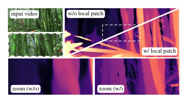
Figure 6: Preservation of low-level details – We ablate the effect of including local patch information into the model’s queries, visualizing the resulting depth maps on an example from the Sintel dataset. We find that the local RGB patches help preserve fine-grained details and produce sharper object boundaries.
| 输入视频 | 无局部图块 / 有局部图块 |
|---|
| 放大(无) / 放大(有) |
|---|
图 6:低层细节的保持——我们消融在模型查询中纳入局部图块信息的效果,并在 Sintel 数据集的一个例子上可视化所得深度图。我们发现,局部 RGB 图块有助于保持细粒度细节,并产生更锐利的物体边界。
| w/ local appear. patch | Video Depth | Camera Pose | |||
|---|---|---|---|---|---|
| AbsRel (S) | AbsRel (SS) | ATE | RPE-T | RPE-R | |
| ✗ | 0.366 | 0.306 | 0.173 | 0.031 | 0.262 |
| ✓ | 0.302 | 0.257 | 0.091 | 0.028 | 0.245 |
Table 7: Local RGB patch – We evaluate a ViT-L model, trained with and without the appearance patch as input to the decoder, on Sintel video depth and camera pose estimation.
| 使用局部外观图块 | 视频深度 | 相机位姿 | |||
|---|---|---|---|---|---|
| AbsRel (S) | AbsRel (SS) | ATE | RPE-T | RPE-R | |
| ✗ | 0.366 | 0.306 | 0.173 | 0.031 | 0.262 |
| ✓ | 0.302 | 0.257 | 0.091 | 0.028 | 0.245 |
表 7:局部 RGB 图块——我们评估一个 ViT-L 模型,分别在解码器输入中使用和不使用外观图块,于 Sintel 上做视频深度和相机位姿估计。
Local RGB patch. As described in Sec. 2.2, we introduce an additional embedding that encodes the local appearance around the query’s source location. This additional embedding yields dramatic performance improvements as shown in Tab. 7 and Fig. 6. These improvements can be attributed to two factors: (i) the local appearance information helps the query establish more reliable correspondences with the encoded spatiotemporal features; and (ii) these patches provide low-level cues that help to segment objects from their surroundings, leading to fine-grained predictions, as exemplified by the sharper depth estimates. We note that while most related works have specialized modules to preserve low level details, such as DPT [37] with its skip connections between encoder and decoder layers, our approach is much simpler. In Appendix C of the appendix, we further highlight how the patches unlock subpixel precision.
局部 RGB 图块。 如第 2.2 节所述,我们引入一个额外嵌入,用于编码查询源位置附近的局部外观。如表 7 和图 6 所示,这一额外嵌入带来了显著的性能提升。改进可归因于两点:(i)局部外观信息帮助查询与已编码的时空特征建立更可靠的对应;(ii)这些图块提供低层线索,有助于把物体从周围环境中分割出来,从而得到更精细的预测,更锐利的深度估计便是例证。我们注意到,多数相关工作用专门模块来保持低层细节,例如 DPT [37] 在编码器与解码器层之间使用跳跃连接,而我们的做法要简单得多。在附录 C 中,我们进一步说明这些图块如何解锁亚像素精度。
Encoder size. We now examine how performance scales with the size of our encoder. Tab. 9 summarizes our findings for ViT-B (90 M) to ViT-g (1 B). As the number of trainable parameters increases, we observe a significant performance improvement, particularly in depth estimation and RPE-R in camera pose estimation.
编码器规模。 我们接着考察性能如何随编码器规模变化。表 9 汇总了从 ViT-B(9,000 万)到 ViT-g(10 亿)的结果。随着可训练参数增多,我们观察到显著的性能提升,在深度估计以及相机位姿估计的 RPE-R 上尤其明显。
| Losses | Video Depth | Camera Pose | |||
|---|---|---|---|---|---|
| AbsRel(S) | AbsRel(SS) | ATE | RPE-T | RPE-R | |
| D4RT | 0.302 | 0.257 | 0.091 | 0.028 | 0.245 |
| w/o 2D position | +0.071 | +0.063 | +0.002 | +0.002 | -0.028 |
| w/o normal | +0.043 | +0.026 | +0.003 | +0.003 | -0.022 |
| w/o displacement | +0.011 | +0.007 | +0.011 | +0.003 | +0.007 |
| w/o visibility | -0.003 | -0.025 | +0.012 | +0.011 | +0.022 |
| w/o confidence | +0.002 | -0.025 | +0.126 | +0.061 | +0.115 |
Table 8: Auxiliary losses – We remove auxiliary losses individually to evaluate their impact on model performance. A slight trade-off between depth and camera estimation pose is observed, though we find that all auxiliary losses improve overall performance.
| 损失 | 视频深度 | 相机位姿 | |||
|---|---|---|---|---|---|
| AbsRel(S) | AbsRel(SS) | ATE | RPE-T | RPE-R | |
| D4RT | 0.302 | 0.257 | 0.091 | 0.028 | 0.245 |
| 去掉二维位置 | +0.071 | +0.063 | +0.002 | +0.002 | -0.028 |
| 去掉法向 | +0.043 | +0.026 | +0.003 | +0.003 | -0.022 |
| 去掉位移 | +0.011 | +0.007 | +0.011 | +0.003 | +0.007 |
| 去掉可见性 | -0.003 | -0.025 | +0.012 | +0.011 | +0.022 |
| 去掉置信度 | +0.002 | -0.025 | +0.126 | +0.061 | +0.115 |
表 8:辅助损失——我们逐项去掉辅助损失,以评估它们对模型性能的影响。深度估计与相机位姿估计之间存在轻微权衡,但我们发现所有辅助损失都改善了总体性能。
| Backbone size | Video Depth | Camera Pose | |||
|---|---|---|---|---|---|
| AbsRel (S) | AbsRel (SS) | ATE | RPE-T | RPE-R | |
| ViT-B | 0.319 | 0.232 | 0.145 | 0.034 | 0.266 |
| ViT-L | 0.256 | 0.214 | 0.073 | 0.027 | 0.191 |
| ViT-H | 0.226 | 0.173 | 0.070 | 0.028 | 0.186 |
| ViT-g | 0.191 | 0.168 | 0.078 | 0.026 | 0.160 |
Table 9: Backbone size – We examine how D4RT’s performance scales with the size of the pretrained ViT encoder backbone, evaluating video depth and camera pose estimation performance on Sintel. We observe a clear improvement as the backbone size increases from ViT-B to ViT-g.
| 骨干规模 | 视频深度 | 相机位姿 | |||
|---|---|---|---|---|---|
| AbsRel (S) | AbsRel (SS) | ATE | RPE-T | RPE-R | |
| ViT-B | 0.319 | 0.232 | 0.145 | 0.034 | 0.266 |
| ViT-L | 0.256 | 0.214 | 0.073 | 0.027 | 0.191 |
| ViT-H | 0.226 | 0.173 | 0.070 | 0.028 | 0.186 |
| ViT-g | 0.191 | 0.168 | 0.078 | 0.026 | 0.160 |
表 9:骨干规模——我们考察 D4RT 的性能如何随预训练 ViT 编码器骨干的规模变化,并在 Sintel 上评估视频深度与相机位姿估计。从 ViT-B 到 ViT-g,可以清楚地看到随骨干增大而提升。
Auxiliary losses. We finally investigate the contribution of each auxiliary loss in Tab. 8. We observe a range of behaviors acros the auxiliary losses: some significantly boost depth performance (e.g., 2D position, normal), others are critical for better camera pose estimation (e.g., confidence), and displacement has small improvements across the board.
辅助损失。 我们最后在表 8 中考察各项辅助损失的贡献。不同辅助损失表现出不同行为:有的显著提升深度性能(例如二维位置、法向),有的对更好的相机位姿估计至关重要(例如置信度),而位移则在各方面都有小幅改进。
5 Conclusion
5 结论
In this work, we introduce D4RT, a simple yet highly scalable feedforward network that reconstructs dynamic 4D scenes with temporal correspondence. Our core innovation is an efficient, query-based decoder that allows for the independent prediction of any point’s 3D position in space and time. This flexible parametrization avoids the computational bottlenecks of dense per-frame decoders, enabling inference that scales linearly with the number of points to be reconstructed. Crucially, we demonstrate that D4RT achieves state-of-the-art results across a wide range of 4D tasks including depth, point cloud estimation, and 3D point tracking. D4RT demonstrates that scaling to complex, dynamic environments does not require sacrificing precision, offering a unified framework for the next generation of 4D perception.
本文提出 D4RT,一种简洁且高度可扩展的前馈网络,能够重建带有时间对应的动态四维场景。核心创新是高效的基于查询的解码器,可以独立预测任意一点在空间与时间中的三维位置。这种灵活的参数化避开了按帧稠密解码的计算瓶颈,使推理成本随待重建点数线性增长。至关重要的是,我们表明 D4RT 在深度、点云估计和三维点跟踪等广泛的四维任务上达到先进水平。D4RT 说明,把规模做到复杂的动态环境,不必以牺牲精度为代价,从而为下一代四维感知提供了一个统一框架。
Contribution and Acknowledgements. MS led the project, with management support from JZ. MS proposed the SRT-style decoder, and GL proposed local RGB patches and tracking-all-pixels. CZ, GL, IR, and MS contributed to the core model design. LM, SS, IR, and SK designed and created training datasets. CZ, GL, and MS carried out the major implementation, with significant contributions from SK, IR, LM, and JX. CZ drove the model experimentation. Comprehensive evaluations and data pipelines were set up by CZ, GL, SK, IR, LM, JX, SS, and MS. Visualizations were produced by GL, IR and JX. RS, JB, RH, ZG, and AZ provided project support, advising, and guidance.
贡献与致谢。 MS 负责主持项目,JZ 提供管理支持。MS 提出了 SRT 风格的解码器,GL 提出了局部 RGB 图块以及跟踪全部像素。CZ、GL、IR 与 MS 参与了核心模型设计。LM、SS、IR 与 SK 设计并创建了训练数据集。CZ、GL 与 MS 承担了主要实现,SK、IR、LM 与 JX 亦有重要贡献。CZ 推动了模型实验。全面的评估与数据流水线由 CZ、GL、SK、IR、LM、JX、SS 与 MS 共同搭建。可视化由 GL、IR 与 JX 完成。RS、JB、RH、ZG 与 AZ 提供了项目支持、建议与指导。
We thank a number of colleagues and advisors for making this work possible. We thank Saurabh Saxena, Kaiming He, Carl Doersch, Leonidas Guibas, Noah Snavely, Ben Poole, Joao Carreira, Pauline Luc, Yi Yang, Howard Huang, Huizhong Chen, Cordelia Schmid for providing advice during the project; Gabriel Brostow, for advising SK during the course of the project and for providing feedback on the manuscript; Relja Aranđelović and Maks Ovsjanikov for providing feedback on the manuscript; Ross Goroshin, Tengda Han and Dilara Gokay for their help during early-stage development; Aravindh Mahendran for helping with code reviews; Daniel Duckworth for helping with visualizations and comparisons against baselines; and Alberto García and Jesús Pérez for the invaluable contributions to data generation and collection.
我们感谢许多同事与顾问使这项工作成为可能。感谢 Saurabh Saxena、Kaiming He、Carl Doersch、Leonidas Guibas、Noah Snavely、Ben Poole、Joao Carreira、Pauline Luc、Yi Yang、Howard Huang、Huizhong Chen、Cordelia Schmid 在项目过程中给予建议;感谢 Gabriel Brostow 在项目期间指导 SK,并对手稿提供反馈;感谢 Relja Aranđelović 与 Maks Ovsjanikov 对手稿提供反馈;感谢 Ross Goroshin、Tengda Han 与 Dilara Gokay 在早期开发中的帮助;感谢 Aravindh Mahendran 协助代码审查;感谢 Daniel Duckworth 协助可视化以及与基线的比较;并感谢 Alberto García 与 Jesús Pérez 在数据生成与采集上的宝贵贡献。
References
参考文献
Appendix
附录
[1] Abhishek Badki, Hang Su, Bowen Wen, and Orazio Gallo. L4P: Towards unified low-level 4D vision perception. In 3DV , 2026.
[2] Daniel J. Butler, Jonas Wulff, Garrett B. Stanley, and Michael J. Black. A naturalistic open source movie for optical flow evaluation. In ECCV , 2012.
[3] Xingyu Chen, Yue Chen, Yuliang Xiu, Andreas Geiger, and Anpei Chen. Easi3r: Estimating disentangled motion from dust3r without training. ICCV , 2025.
[4] Angela Dai, Angel X. Chang, Manolis Savva, Maciej Halber, Thomas Funkhouser, and Matthias Nießner. Scannet: Richly-annotated 3d reconstructions of indoor scenes. In CVPR , 2017a.
[5] Angela Dai, Angel X. Chang, Manolis Savva, Maciej Halber, Thomas Funkhouser, and Matthias Nießner. ScanNet: Richly-annotated 3D reconstructions of indoor scenes. In CVPR , 2017b.
[6] Kai Deng, Zexin Ti, Jiawei Xu, Jian Yang, and Jin Xie. VGGT-Long: Chunk it, loop it, align it – pushing VGGT’s limits on kilometer-scale long RGB sequences. arXiv preprint , 2025.
[7] Carl Doersch, Ankush Gupta, Larisa Markeeva, Adria Recasens, Lucas Smaira, Yusuf Aytar, Joao Carreira, Andrew Zisserman, and Yi Yang. Tap-vid: A benchmark for tracking any point in a video. NeurIPS , 2022.
[8] Carl Doersch, Yi Yang, Mel Vecerik, Dilara Gokay, Ankush Gupta, Yusuf Aytar, Joao Carreira, and Andrew Zisserman. Tapir: Tracking any point with per-frame initialization and temporal refinement. In ICCV , 2023.
[9] Alexey Dosovitskiy, Lucas Beyer, Alexander Kolesnikov, Dirk Weissenborn, Xiaohua Zhai, Thomas Unterthiner, Mostafa Dehghani, Matthias Minderer, Georg Heigold, Sylvain Gelly, Jakob Uszkoreit, and Neil Houlsby. An image is worth 16x16 words: Transformers for image recognition at scale. In ICLR , 2021.
[10] David Eigen, Christian Puhrsch, and Rob Fergus. Depth map prediction from a single image using a multi-scale deep network. In NeurIPS , 2014.
[11] Haiwen Feng, Junyi Zhang, Qianqian Wang, Yufei Ye, Pengcheng Yu, Michael J Black, Trevor Darrell, and Angjoo Kanazawa. St4rtrack: Simultaneous 4d reconstruction and tracking in the world. ICCV , 2025.
[12] Yasutaka Furukawa, Carlos Hernández, et al. Multi-view stereo: A tutorial. Foundations and trends® in Computer Graphics and Vision , 2015.
[13] A Gaidon, Q Wang, Y Cabon, and E Vig. Virtual worlds as proxy for multi-object tracking analysis. In CVPR , 2016.
[14] Andreas Geiger, Philip Lenz, Christoph Stiller, and Raquel Urtasun. Vision meets robotics: The KITTI dataset. IJRR , 2013.
[15] Klaus Greff, Etienne Pot, and Mehdi S. M. Sajjadi. Kauldron: A neural network training framework, optimized for research velocity and modularity. https://github.com/google-research/kauldron .
[16] Klaus Greff, Francois Belletti, Lucas Beyer, Carl Doersch, Yilun Du, Daniel Duckworth, David J Fleet, Dan Gnanapragasam, Florian Golemo, Charles Herrmann, et al. Kubric: A scalable dataset generator. In CVPR , 2022.
[17] Adam W Harley, Zhaoyuan Fang, and Katerina Fragkiadaki. Particle video revisited: Tracking through occlusions using point trajectories. In ECCV , 2022.
[18] Adam W. Harley, Yang You, Xinglong Sun, Yang Zheng, Nikhil Raghuraman, Yunqi Gu, Sheldon Liang, Wen-Hsuan Chu, Achal Dave, Pavel Tokmakov, Suya You, Rares Ambrus, Katerina Fragkiadaki, and Leonidas J. Guibas. AllTracker: Efficient dense point tracking at high resolution. In ICCV , 2025.
[19] Richard Hartley and Andrew Zisserman. Multiple view geometry in computer vision . Cambridge university press, 2003.
[20] Po-Han Huang, Kevin Matzen, Johannes Kopf, Narendra Ahuja, and Jia-Bin Huang. Deepmvs: Learning multi-view stereopsis. In CVPR , 2018.
[21] Zeren Jiang, Chuanxia Zheng, Iro Laina, Diane Larlus, and Andrea Vedaldi. Geo4d: Leveraging video generators for geometric 4d scene reconstruction. In ICCV , 2025.
[22] Nikita Karaev, Ignacio Rocco, Benjamin Graham, Natalia Neverova, Andrea Vedaldi, and Christian Rupprecht. Dynamicstereo: Consistent dynamic depth from stereo videos. In CVPR , 2023.
[23] Nikita Karaev, Yuri Makarov, Jianyuan Wang, Natalia Neverova, Andrea Vedaldi, and Christian Rupprecht. Cotracker3: Simpler and better point tracking by pseudo-labelling real videos. In ICCV , 2025.
[24] Nikhil Keetha, Norman Müller, Johannes Schönberger, Lorenzo Porzi, Yuchen Zhang, Tobias Fischer, Arno Knapitsch, Duncan Zauss, Ethan Weber, Nelson Antunes, et al. Mapanything: Universal feed-forward metric 3d reconstruction. arXiv preprint , 2025.
[25] Alex Kendall and Yarin Gal. What uncertainties do we need in bayesian deep learning for computer vision? In NeurIPS , 2017.
[26] Diederik P Kingma. Adam: A method for stochastic optimization. ICLR , 2015.
[27] Skanda Koppula, Ignacio Rocco, Yi Yang, Joe Heyward, Joao Carreira, Andrew Zisserman, Gabriel Brostow, and Carl Doersch. Tapvid-3d: A benchmark for tracking any point in 3d. In NeurIPS , 2024.
[28] Guillaume Le Moing, Jean Ponce, and Cordelia Schmid. Dense optical tracking: Connecting the dots. In CVPR , 2024.
[29] Zhengqi Li, Richard Tucker, Forrester Cole, Qianqian Wang, Linyi Jin, Vickie Ye, Angjoo Kanazawa, Aleksander Holynski, and Noah Snavely. MegaSaM: Accurate, fast and robust structure and motion from casual dynamic videos. In CVPR , 2025.
[30] Ilya Loshchilov and Frank Hutter. Decoupled weight decay regularization. ICLR , 2019.
[31] Jiahao Lu, Tianyu Huang, Peng Li, Zhiyang Dou, Cheng Lin, Zhiming Cui, Zhen Dong, Sai-Kit Yeung, Wenping Wang, and Yuan Liu. Align3r: Aligned monocular depth estimation for dynamic videos. In CVPR , 2025.
[32] Tuan Duc Ngo, Peiye Zhuang, Chuang Gan, Evangelos Kalogerakis, Sergey Tulyakov, Hsin-Ying Lee, and Chaoyang Wang. Delta: Dense efficient long-range 3d tracking for any video. ICLR , 2025.
[33] John Oliensis. A critique of structure-from-motion algorithms. CVIU , 2000.
[34] Emanuele Palazzolo, Jens Behley, Philipp Lottes, Philippe Giguère, and Cyrill Stachniss. Refusion: 3d reconstruction in dynamic environments for rgb-d cameras exploiting residuals. In IROS , 2019.
[35] Duc-Hai Pham, Tung Do, Phong Nguyen, Binh-Son Hua, Khoi Nguyen, and Rang Nguyen. SharpDepth: Sharpening metric depth predictions using diffusion distillation. In CVPR , 2025.
[36] Luigi Piccinelli, Christos Sakaridis, Yung-Hsu Yang, Mattia Segu, Siyuan Li, Wim Abbeloos, and Luc Van Gool. UniDepthV2: Universal Monocular Metric Depth Estimation Made Simpler. PAMI , 2025.
[37] René Ranftl, Alexey Bochkovskiy, and Vladlen Koltun. Vision transformers for dense prediction. ICCV , 2021.
[38] Jeremy Reizenstein, Roman Shapovalov, Philipp Henzler, Luca Sbordone, Patrick Labatut, and David Novotny. Common objects in 3d: Large-scale learning and evaluation of real-life 3d category reconstruction. In ICCV , 2021.
[39] Mehdi SM Sajjadi, Henning Meyer, Etienne Pot, Urs Bergmann, Klaus Greff, Noha Radwan, Suhani Vora, Mario Lučić, Daniel Duckworth, Alexey Dosovitskiy, et al. Scene representation transformer: Geometry-free novel view synthesis through set-latent scene representations. In CVPR , 2022.
[40] Mehdi S. M. Sajjadi, Aravindh Mahendran, Thomas Kipf, Etienne Pot, Daniel Duckworth, Mario Lučić, and Klaus Greff. RUST: Latent Neural Scene Representations from Unposed Imagery. CVPR , 2023.
[41] Peter Sand and Seth Teller. Particle video: Long-range motion estimation using point trajectories. IJCV , 2008.
[42] Johannes L Schonberger and Jan-Michael Frahm. Structure-from-motion revisited. In CVPR , 2016.
[43] Johannes L Schönberger, Enliang Zheng, Jan-Michael Frahm, and Marc Pollefeys. Pixelwise view selection for unstructured multi-view stereo. In ECCV , 2016.
[44] Edgar Sucar, Zihang Lai, Eldar Insafutdinov, and Andrea Vedaldi. Dynamic point maps: A versatile representation for dynamic 3d reconstruction. arXiv preprint arXiv:2503.16318 , 2025.
[45] Pei Sun, Henrik Kretzschmar, Xerxes Dotiwalla, Aurelien Chouard, Vijaysai Patnaik, Paul Tsui, James Guo, Yin Zhou, Yuning Chai, Benjamin Caine, Vijay Vasudevan, Wei Han, Jiquan Ngiam, Hang Zhao, Aleksei Timofeev, Scott Ettinger, Maxim Krivokon, Amy Gao, Aditya Joshi, Yu Zhang, Jonathon Shlens, Zhifeng Chen, and Dragomir Anguelov. Scalability in perception for autonomous driving: Waymo open dataset. In CVPR , 2020.
[46] Shinji Umeyama. Least-squares estimation of transformation parameters between two point patterns. TPAMI , 1991.
[47] Ashish Vaswani, Noam Shazeer, Niki Parmar, Jakob Uszkoreit, Llion Jones, Aidan N Gomez, Ł ukasz Kaiser, and Illia Polosukhin. Attention is all you need. In NeurIPS , 2017.
[48] Jianyuan Wang, Minghao Chen, Nikita Karaev, Andrea Vedaldi, Christian Rupprecht, and David Novotny. Vggt: Visual geometry grounded transformer. In CVPR , 2025a.
[49] Limin Wang, Bingkun Huang, Zhiyu Zhao, Zhan Tong, Yinan He, Yi Wang, Yali Wang, and Yu Qiao. VideoMAE v2: Scaling video masked autoencoders with dual masking. In CVPR , 2023.
[50] Qianqian Wang, Yifei Zhang, Aleksander Holynski, Alexei A Efros, and Angjoo Kanazawa. Continuous 3d perception model with persistent state. In CVPR , 2025b.
[51] Shuzhe Wang, Vincent Leroy, Yohann Cabon, Boris Chidlovskii, and Jerome Revaud. Dust3r: Geometric 3d vision made easy. In CVPR , 2024.
[52] Shizun Wang, Zhenxiang Jiang, Xingyi Yang, and Xinchao Wang. C4d: 4d made from 3d through dual correspondences. In ICCV , 2025c.
[53] Wenshan Wang, Delong Zhu, Xiangwei Wang, Yaoyu Hu, Yuheng Qiu, Chen Wang, Yafei Hu, Ashish Kapoor, and Sebastian Scherer. TartanAir: A dataset to push the limits of visual slam. In IROS , 2020.
[54] Yifan Wang, Jianjun Zhou, Haoyi Zhu, Wenzheng Chang, Yang Zhou, Zizun Li, Junyi Chen, Jiangmiao Pang, Chunhua Shen, and Tong He. p i 3 pi^{3} : Permutation-equivariant visual geometry learning. arXiv preprint , 2025d.
[55] Yuxi Xiao, Qianqian Wang, Shangzhan Zhang, Nan Xue, Sida Peng, Yujun Shen, and Xiaowei Zhou. Spatialtracker: Tracking any 2d pixels in 3d space. In CVPR , 2024.
[56] Yuxi Xiao, Jianyuan Wang, Nan Xue, Nikita Karaev, Yuri Makarov, Bingyi Kang, Xing Zhu, Hujun Bao, Yujun Shen, and Xiaowei Zhou. SpatialTrackerV2: Advancing 3d point tracking with explicit camera motion. In ICCV , 2025.
[57] Jianing Yang, Alexander Sax, Kevin J Liang, Mikael Henaff, Hao Tang, Ang Cao, Joyce Chai, Franziska Meier, and Matt Feiszli. Fast3r: Towards 3d reconstruction of 1000+ images in one forward pass. In CVPR , 2025.
[58] Yao Yao, Zixin Luo, Shiwei Li, Jingyang Zhang, Yufan Ren, Lei Zhou, Tian Fang, and Long Quan. Blendedmvs: A large-scale dataset for generalized multi-view stereo networks. In CVPR , 2020.
[59] Chandan Yeshwanth, Yueh-Cheng Liu, Matthias Nießner, and Angela Dai. Scannet++: A high-fidelity dataset of 3d indoor scenes. In ICCV , 2023.
[60] Junyi Zhang, Charles Herrmann, Junhwa Hur, Varun Jampani, Trevor Darrell, Forrester Cole, Deqing Sun, and Ming-Hsuan Yang. Monst3r: A simple approach for estimating geometry in the presence of motion. ICLR , 2025.
[61] Zhengyou Zhang. A flexible new technique for camera calibration. TPAMI , 2002.
[62] Yang Zheng, Adam W. Harley, Bokui Shen, Gordon Wetzstein, and Leonidas J. Guibas. Pointodyssey: A large-scale synthetic dataset for long-term point tracking. In ICCV , 2023.
[63] Artem Zholus, Carl Doersch, Yi Yang, Skanda Koppula, Viorica Patraucean, Xu Owen He, Ignacio Rocco, Mehdi SM Sajjadi, Sarath Chandar, and Ross Goroshin. TAPNext: Tracking any point as next token prediction. In ICCV , 2025.
Appendix A Model Overview & Training Details
附录 A 模型概览与训练细节
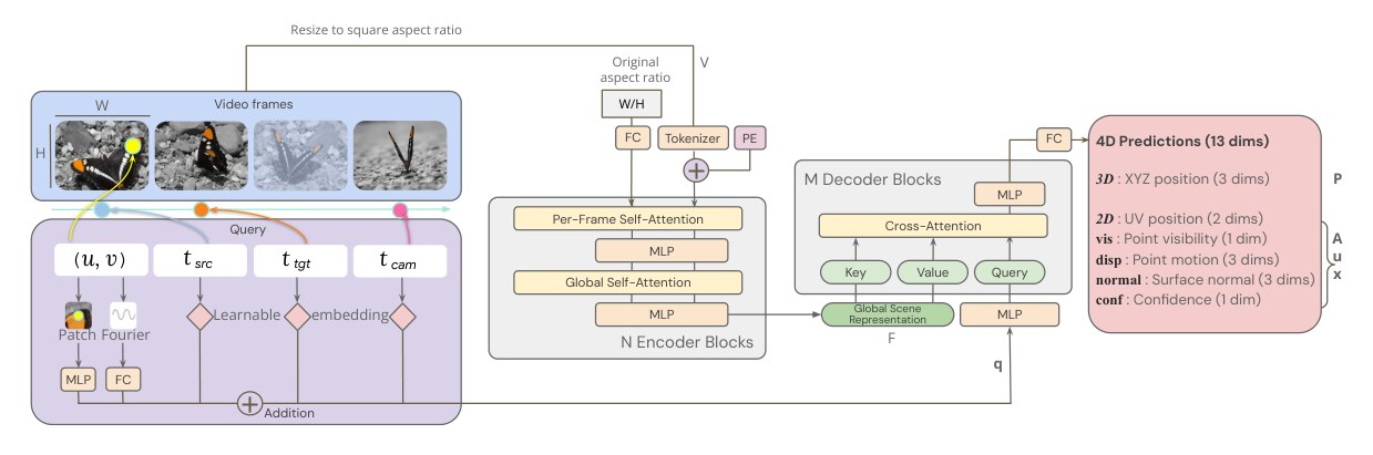
Figure 7: Full D4RT model overview – We provide a holistic overview of the model together with its inputs and outputs. FC corresponds to a fully connected layer, and PE for positional encoding. See Sec. 2 of the main paper for reference.
图 7:完整的 D4RT 模型概览——我们给出模型及其输入、输出的整体概览。FC 表示全连接层,PE 表示位置编码。参见正文第 2 节。
The model is trained end-to-end by minimizing a composite loss , which is a weighted sum of task-specific losses computed over a batch of sampled queries:
模型通过最小化复合损失 进行端到端训练,该损失是在一批 个采样查询上计算的各任务损失的加权和:
where is the confidence score predicted by the model. We use the following loss weights: , , , , , , . We train using the AdamW optimizer with a weight decay of . The learning rate is warmed up for steps until it reaches a peak value of . Subsequently, it follows a cosine annealing schedule, decaying to a final value of . Gradients are clipped to a maximum -norm of .
其中 是模型预测的置信度分数。我们使用如下损失权重:,,,,,,。训练使用 AdamW 优化器,权重衰减为 。学习率先预热 步,达到峰值 ,随后按余弦退火日程衰减到终值 。梯度按最大 范数 进行裁剪。
Data augmentation.
Extensive data augmentation techniques are applied to the video during training to improve model generalization. We apply temporally consistent color jittering by performing random brightness, saturation, contrast, and hue adjustments. We also apply random color drop with a probability of , and Gaussian blur augmentation with a probability of . For spatial augmentation, we use random crop augmentations with a scale ratio between and of the original size. After determining the crop size, a random aspect ratio is selected by sampling from a uniform distribution in the logarithmic domain; this ensures equal probability for wide and tall crops while respecting image boundaries. Additionally, during the random crop augmentation, the image is randomly zoomed in with a probability of . On the temporal dimension, frames are subsampled from the full video with a random stride.
数据增强。
训练中对视频施加大量数据增强,以改善模型泛化。我们做时间一致的颜色抖动,随机调整亮度、饱和度、对比度和色相。还以 的概率随机去掉颜色,并以 的概率做高斯模糊增强。空间增强方面,我们使用随机裁剪,尺度比在原尺寸的 到 之间。确定裁剪尺寸后,再从对数域的均匀分布中采样随机长宽比;这样可以在遵守图像边界的同时,使宽幅与高幅裁剪具有相等概率。此外,在随机裁剪增强中,图像还会以 的概率被随机放大。在时间维上,从完整视频中以随机步长对帧做子采样。
Training queries.
Queries are sampled from available ground truth point trajectories. To focus the model on challenging regions, of the queries (along dimensions ) are sampled near depth discontinuities or motion boundaries, which are pre-computed using a Sobel filter on depth maps. Timesteps , , and are sampled uniformly at random, except that we enforce with probability to improve downstream performance.
训练查询。
查询从可用的真值点轨迹中采样。为使模型关注困难区域,沿 维有 的查询采样自深度间断或运动边界附近,这些位置事先用 Sobel 滤波器在深度图上计算得到。时刻 、 和 均匀随机采样,但我们以 的概率强制 ,以改善下游性能。
Appendix B Generalization to Long Videos
附录 B 向长视频的泛化
We implement a long-sequence processing algorithm by partitioning videos into overlapping segments. We then align these segments by estimating Sim(3) transformations using the Umeyama algorithm [46], based on the top 85% of points with the highest confidence in the overlapping regions. The process is similar to the first stage proposed in VGGT-Long [6], we omit loop detection and optimization stage in [6] to directly evaluate the reconstruction model’s raw precision. As shown in Fig. 8 on KITTI [14], our model yields the best ATE in the first example, significantly outperforming VGG-T and by a large margin. On the second example, we significantly outperform VGG-T and produce a result on par with .
我们实现了一种长序列处理算法,把视频划分成相互重叠的片段,再用 Umeyama 算法 [46] 估计 Sim(3) 变换来对齐这些片段,依据是重叠区域中置信度最高的前 85% 的点。这一过程类似于 VGGT-Long [6] 提出的第一阶段;我们省略了 [6] 中的回环检测与优化阶段,以便直接评估重建模型的原始精度。如图 8 在 KITTI [14] 上所示,本模型在第一个例子中取得最好的 ATE,大幅超过 VGG-T 和 。在第二个例子中,我们明显超过 VGG-T,并得到与 相当的结果。
(a) Visualization of reconstruction of 1000 frames from KITTI sequence 00.
(b) Comparison of raw chunked prediction alignment results against VGG-T and baselines (no loop closure).
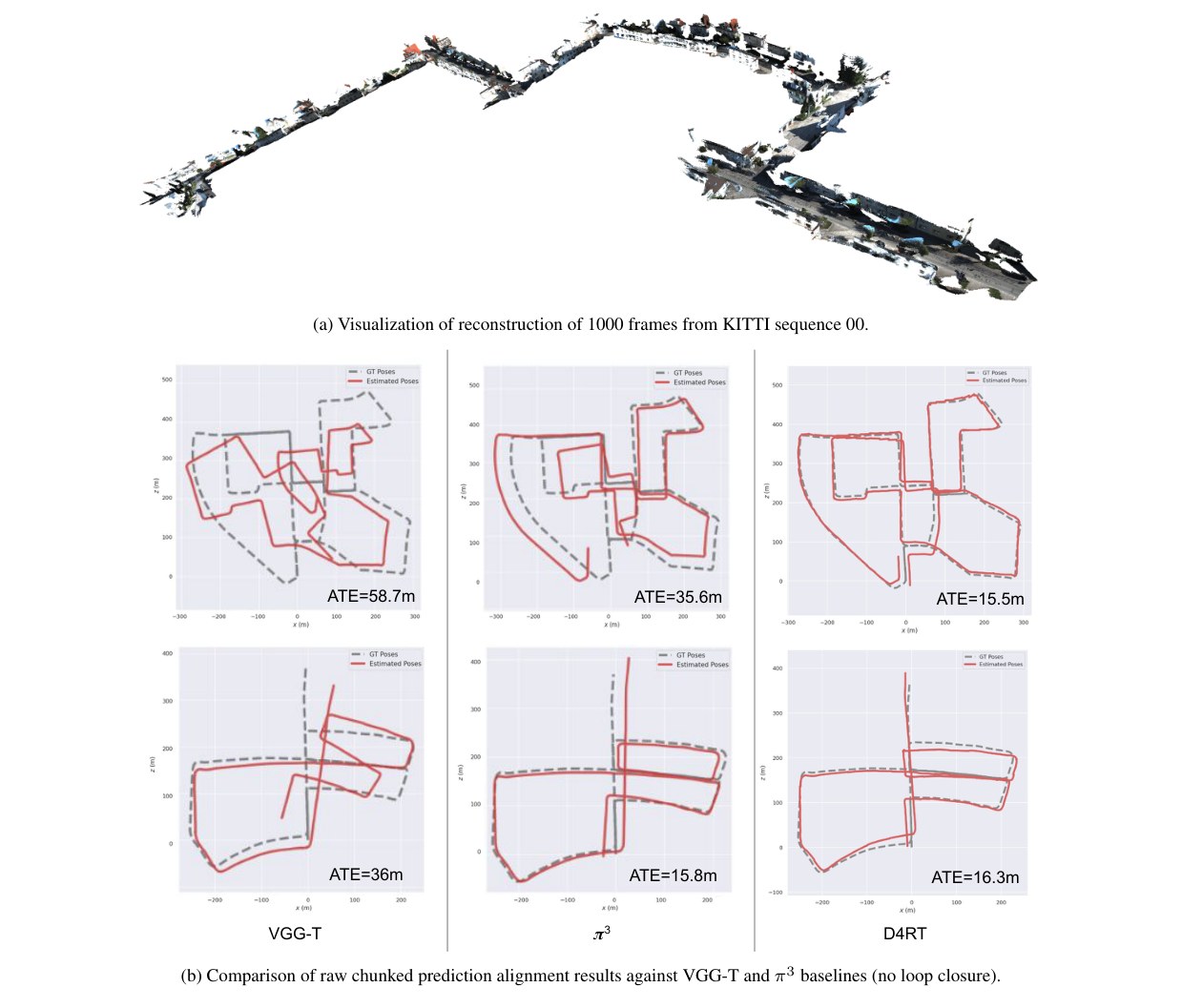
Figure 8: Long sequence results on KITTI sequences – We align and stitch predictions from overlapped chunks by Umeyama algorithm, without the loop detection and global optimization proposed in [6]. Our model obtains consistently better results than VGG-T, and significantly better results than on sequence “00” (top row).
(a) 对 KITTI 序列 00 中 1000 帧重建的可视化。
(b) 将原始分块预测对齐结果与 VGG-T 及 基线比较(无回环闭合)。
图 8:KITTI 序列上的长序列结果——我们用 Umeyama 算法对齐并拼接来自重叠片段的预测,不使用 [6] 中提出的回环检测与全局优化。本模型结果稳定优于 VGG-T,并在序列 “00”(上行)上明显优于 。
Appendix C High-Resolution Decoding with Subpixel Precision
附录 C 具有亚像素精度的高分辨率解码
A key advantage of D4RT’s architecture is the decoupling of the global scene encoding from the point-wise decoding. As the query coordinates are defined in a continuous normalized space , our decoder is able to probe the scene at arbitrary resolutions, independent of the resolution of the Global Scene Representation .
D4RT 架构的一个关键优势,是把全局场景编码与逐点解码解耦。由于查询坐标 定义在连续的归一化空间 中,解码器可以在任意分辨率下探测场景,而不受全局场景表示 分辨率的限制。
We explore this capability in Tab. 10. To quantify the preservation of high-frequency details, we report the Pseudo Depth Boundary Error accuracy () proposed by Pham et al. [35], in addition to standard depth metrics. We compare four configurations using a ViT-g encoder fixed at a resolution of . The baseline output at the encoder’s native resolution (Config \scriptsize1⃝) is naturally coarse. Incorporating the local appearance patch mechanism described in the main paper (Config \scriptsize2⃝) allows for the recovery of finer low-level structures, although pixelation artifacts persist. We further leverage the continuous nature of our query mechanism to predict at the original resolution. While naive dense querying (Config \scriptsize3⃝) recovers smoother edges, it still fails at recovering high frequencies.
我们在表 10 中探索这一能力。为量化高频细节的保持,除标准深度指标外,我们还报告 Pham 等人 [35] 提出的伪深度边界误差准确率()。比较在编码器分辨率固定为 的 ViT-g 上的四种配置。编码器原生分辨率下的基线输出(配置 ①)自然较粗。纳入正文所述的局部外观图块机制(配置 ②)可以恢复更细的低层结构,但像素化伪影仍然存在。我们进一步利用查询机制的连续性,在原始分辨率上预测。虽然朴素的稠密查询(配置 ③)能恢复更平滑的边缘,但仍然无法恢复高频成分。
In Config \scriptsize4⃝, we extract the local RGB patches from the source frames at their original resolution for decoding.
在配置 ④中,我们从源帧的原始分辨率提取局部 RGB 图块,再用于解码。
The significant drop in demonstrates how this allows D4RT to recover finer details. We show qualitative results in Fig. 9 where we observe that hair strands and object boundaries are resolved more accurately.
的显著下降表明,这使 D4RT 能够恢复更细的细节。我们在图 9 中给出定性结果,可以看到发丝和物体边界被更准确地分辨出来。
| Config. | Encoder Resolution | RGB Patch | Output Resolution | RGB patch Resolution | Scale | Scale and Shift | ||
|---|---|---|---|---|---|---|---|---|
| AbsRel | AbsRel | |||||||
| \scriptsize1⃝ | ✗ | 0.254 | 3.323 | 0.219 | 3.307 | |||
| \scriptsize2⃝ | ✓ | 0.218 | 2.254 | 0.179 | 2.243 | |||
| \scriptsize3⃝ | ✓ | Original | 0.217 | 2.266 | 0.178 | 2.258 | ||
| \scriptsize4⃝ | ✓ | Original | Original | 0.220 | 2.193 | 0.176 | 2.185 |
Table 10: Quantitative impact of query density and patch fidelity – Feeding RGB patches from the high-resolution video into the decoder (Config \scriptsize4⃝) yields significantly sharper edges in depth maps as measured by .
| 配置 | 编码器分辨率 | RGB 图块 | 输出分辨率 | RGB 图块分辨率 | 尺度 | 尺度与平移 | ||
|---|---|---|---|---|---|---|---|---|
| AbsRel | AbsRel | |||||||
| ① | ✗ | 0.254 | 3.323 | 0.219 | 3.307 | |||
| ② | ✓ | 0.218 | 2.254 | 0.179 | 2.243 | |||
| ③ | ✓ | 原始 | 0.217 | 2.266 | 0.178 | 2.258 | ||
| ④ | ✓ | 原始 | 原始 | 0.220 | 2.193 | 0.176 | 2.185 |
表 10:查询密度与图块保真度的定量影响——把高分辨率视频中的 RGB 图块送入解码器(配置 ④),按 衡量,深度图的边缘明显更锐利。
| Input video | Config \scriptsize1⃝ | Config \scriptsize2⃝ | Config \scriptsize3⃝ | Config \scriptsize4⃝ | GT Depth |
|---|---|---|---|---|---|
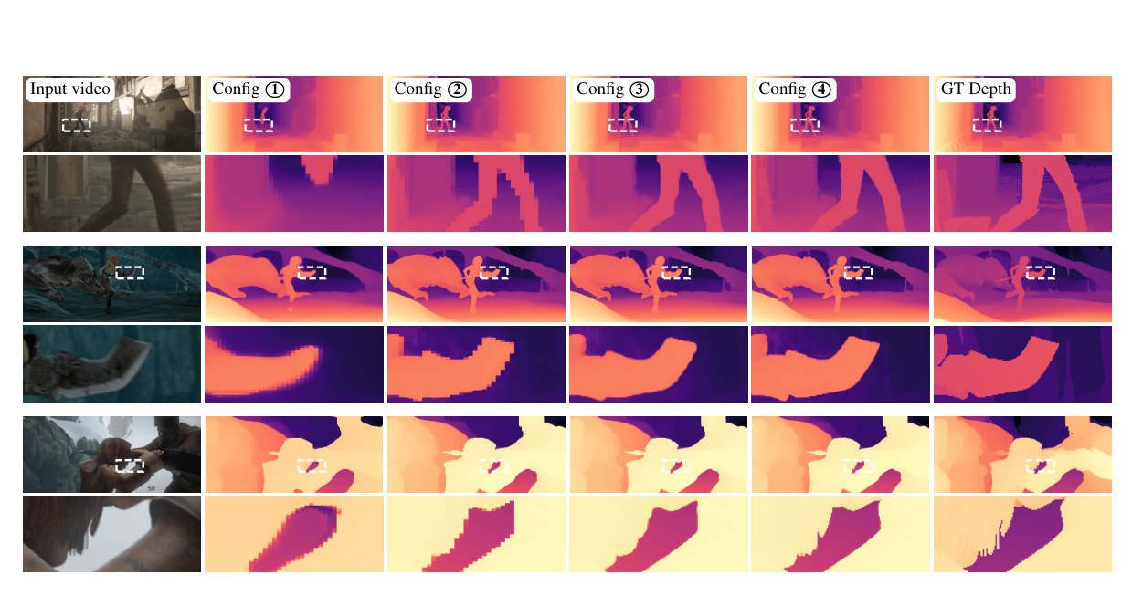
Figure 9: Visualizing sub-pixel detail recovery – We propose a visual comparison of the different high-res configurations. Config \scriptsize4⃝ achieves the highest fidelity, it preserves sharp edges and recovers fine details—such as the hair in the bottom row—without increasing the computational cost or memory requirements of the overall model.
| 输入视频 | 配置 ① | 配置 ② | 配置 ③ | 配置 ④ | 真值深度 |
|---|
图 9:可视化亚像素细节恢复——我们对不同的高分辨率配置做可视化比较。配置 ④ 保真度最高,能够保持锐利边缘并恢复细小细节——如下行的头发——同时不增加整体模型的计算成本或显存需求。
Appendix D Further Ablations
附录 D 更多消融
Pretrained Encoder.
In Tab. 11, we show our model performance when the video encoder is initialized with random weights compared to using pre-trained VideoMAE [49] weights. We observe significant improvements across the board.
预训练编码器。
表 11 比较了视频编码器以随机权重初始化、与使用预训练 VideoMAE [49] 权重时的模型性能。我们在各项指标上都观察到显著提升。
| Model weight initialization | Video Depth Estimation | Camera Pose Estimation | |||
|---|---|---|---|---|---|
| AbsRel (S) | AbsRel (SS) | ATE | RPE-T | RPE-R | |
| None | 0.738 | 0.520 | 0.334 | 0.139 | 1.126 |
| VideoMAE [49] | 0.302 | 0.257 | 0.091 | 0.028 | 0.245 |
Table 11: Model initialization – Initializing the model with VideoMAE [49] weights leads to significant improvements.
| 模型权重初始化 | 视频深度估计 | 相机位姿估计 | |||
|---|---|---|---|---|---|
| AbsRel (S) | AbsRel (SS) | ATE | RPE-T | RPE-R | |
| 无 | 0.738 | 0.520 | 0.334 | 0.139 | 1.126 |
| VideoMAE [49] | 0.302 | 0.257 | 0.091 | 0.028 | 0.245 |
表 11:模型初始化——用 VideoMAE [49] 权重初始化模型,会带来显著改进。
Local RGB patch size.
We perform an ablation study on the size of the local RGB patch. As shown in Fig. 10, our results indicate that the patch size 99 yields the best overall performance across camera pose and depth estimation tasks.
局部 RGB 图块尺寸。
我们对局部 RGB 图块的尺寸做了消融。如图 10 所示,结果表明 的图块尺寸在相机位姿和深度估计任务上总体表现最好。
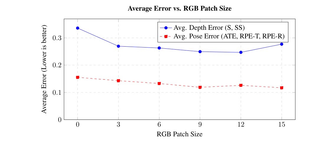
Figure 10: Ablation study on RGB patch size – The plot shows the average error for depth and pose estimation on Sintel. A patch size between 9 and 12 yields the best performance for both tasks.
图 10:关于 RGB 图块尺寸的消融——图中给出 Sintel 上深度与位姿估计的平均误差。图块尺寸在 9 到 12 之间时,两项任务的表现都最好。
Appendix E Further Qualitative Results
附录 E 更多定性结果
Complementing the qualitative visualizations in the main text, we provide additional examples of our reconstruction results in Fig. 11, along with further baseline comparisons in Fig. 12 and Fig. 13.
作为对正文定性可视化的补充,我们在图 11 中提供更多重建结果示例,并在图 12 和图 13 中给出进一步的基线比较。
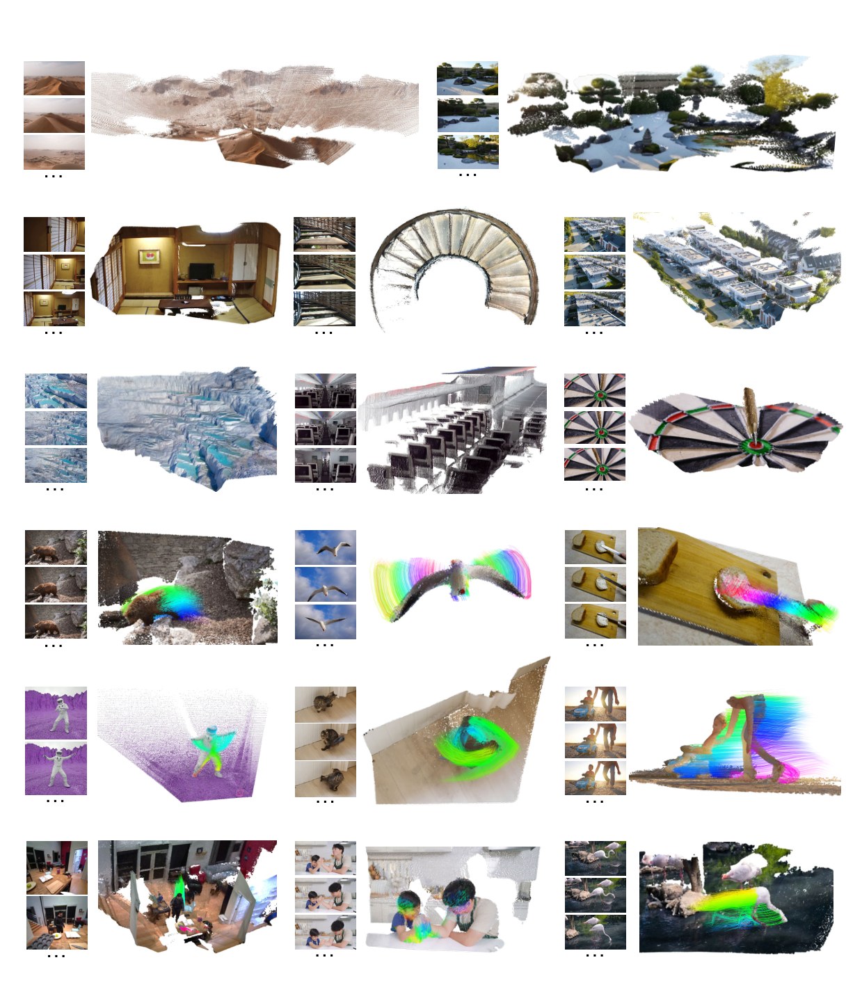
Figure 11: Additional visualizations of D4RT – D4RT produces accurate reconstructions for both static environments (top three rows) and dynamic sequences (bottom three rows).
图 11:D4RT 的更多可视化——D4RT 对静态环境(上三行)和动态序列(下三行)都能给出准确重建。
| Input video | MegaSaM [29] | [54] | SpatialTrackerV2 [56] | D4RT (Ours) |
|---|
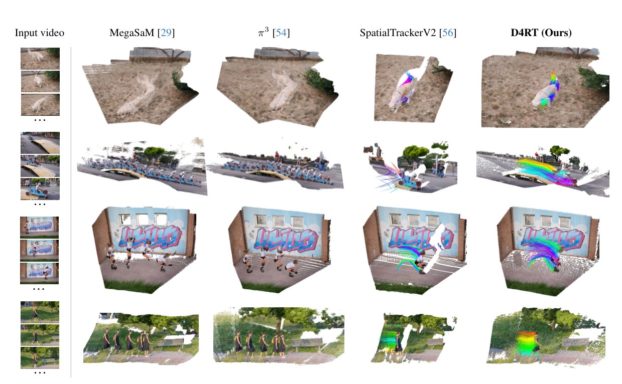
Figure 12: Additional reconstruction results across methods – Pure reconstruction methods (MegaSaM and ) are visualized as accumulated point clouds. For SpatialTrackerV2, we visualize sparse tracks on a representative frame. In contrast, D4RT reconstructs a complete 4D scene representation, tracking all pixels across the entire video.
| 输入视频 | MegaSaM [29] | [54] | SpatialTrackerV2 [56] | D4RT(本文) |
|---|
图 12:各方法的更多重建结果——纯重建方法(MegaSaM 与 )可视化为累加点云。对 SpatialTrackerV2,我们在一帧代表性画面上可视化稀疏轨迹。相比之下,D4RT 重建出完整的四维场景表示,跟踪整段视频中的所有像素。
| Input video | MegaSaM | SpatialTrackerV2 | D4RT (Ours) | |
|---|---|---|---|---|
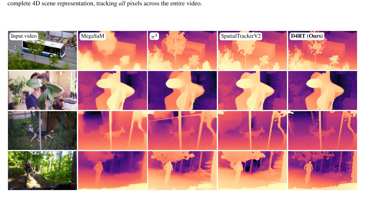
Figure 13: Qualitative depth comparison across methods – D4RT is able to perform dense depth estimation with finer details than current state-of-the-art methods, preserving geometric accuracy even in scenarios with large motion blur.
| 输入视频 | MegaSaM | SpatialTrackerV2 | D4RT(本文) |
|---|
图 13:各方法的定性深度比较——D4RT 能够进行比当前先进方法更细的稠密深度估计,即便在运动模糊很大的情形下也能保持几何精度。