Unpaired Image-to-Image Translation using Cycle-Consistent Adversarial Networks

用循环一致对抗网络做无配对图像到图像翻译（Unpaired Image-to-Image Translation using Cycle-Consistent Adversarial Networks）

Jun-Yan Zhu Thanks:  empty    Taesung Park 1 1 footnotemark: 1    Phillip Isola    Alexei A. Efros    Berkeley AI Research (BAIR) laboratory    UC Berkeley

Jun-Yan Zhu　　Taesung Park　　Phillip Isola　　Alexei A. Efros
Berkeley AI Research（BAIR）实验室，加州大学伯克利分校

Abstract

摘要

Image-to-image translation is a class of vision and graphics problems where the goal is to learn the mapping between an input image and an output image using a training set of aligned image pairs. However, for many tasks, paired training data will not be available. We present an approach for learning to translate an image from a source domain $X$ to a target domain $Y$ in the absence of paired examples. Our goal is to learn a mapping $G:X\rightarrow Y$ such that the distribution of images from $G(X)$ is indistinguishable from the distribution $Y$ using an adversarial loss. Because this mapping is highly under-constrained, we couple it with an inverse mapping $F:Y\rightarrow X$ and introduce a cycle consistency loss to enforce $F(G(X))\approx X$ (and vice versa). Qualitative results are presented on several tasks where paired training data does not exist, including collection style transfer, object transfiguration, season transfer, photo enhancement, etc. Quantitative comparisons against several prior methods demonstrate the superiority of our approach.

图像到图像翻译是一类视觉与图形问题：目标是在成对对齐的图像训练集上学习输入图像到输出图像的映射。然而许多任务无法获得成对训练数据。我们提出一种在缺少配对样例时，把图像从源域 $X$ 转换到目标域 $Y$ 的方法。目标是学习映射 $G:X\to Y$，使 $G(X)$ 的分布与 $Y$ 用对抗损失不可区分。由于这种映射高度欠定，我们再耦合一个逆映射 $F:Y\to X$，并引入循环一致性损失以强制 $F(G(X))\approx X$（反之亦然）。定性和定量结果表明，该方法可在缺少配对训练数据时完成风格迁移、物体变形、季节变换与照片增强等任务。代码见 https://github.com/junyanz/CycleGAN。

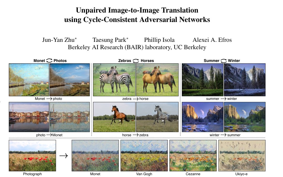
Figure 1: Given any two unordered image collections $X$ and $Y$, our algorithm learns to automatically “translate” an image from one into the other and vice versa: (left) Monet paintings and landscape photos from Flickr; (center) zebras and horses from ImageNet; (right) summer and winter Yosemite photos from Flickr. Example application (bottom): using a collection of paintings of famous artists, our method learns to render natural photographs into the respective styles.

图 1：给定任意两个无序图像集合 $X$ 与 $Y$，我们的算法学习自动把一幅图像“翻译”到另一个集合，并反过来亦然：（左）Flickr 风景照片与莫奈画作；（中）ImageNet 上的斑马与马；（右）Flickr 上约塞米蒂的夏冬照片。示例应用（底行）：用某位著名画家的画作集合，我们的方法学习把照片渲染成该画家的风格。

1 Introduction

1 引言

What did Claude Monet see as he placed his easel by the bank of the Seine near Argenteuil on a lovely spring day in 1873 (Figure 1, top-left)? A color photograph, had it been invented, may have documented a crisp blue sky and a glassy river reflecting it. Monet conveyed his impression of this same scene through wispy brush strokes and a bright palette.[^†]

1873 年一个可爱的春日，克劳德·莫奈 (Claude Monet) 将画架放在阿让特伊 (Argenteuil) 附近的塞纳河畔时，看到了什么（图 1，左上）？ 如果彩色照片被发明的话，它可能记录了蔚蓝的天空和倒映着天空的玻璃般的河流。 莫奈通过纤细的笔触和明亮的调色板传达了他对同一场景的“印象”。[^†]

What if Monet had happened upon the little harbor in Cassis on a cool summer evening (Figure 1, bottom-left)? A brief stroll through a gallery of Monet paintings makes it possible to imagine how he would have rendered the scene: perhaps in pastel shades, with abrupt dabs of paint, and a somewhat flattened dynamic range.

如果莫奈在一个凉爽的夏夜偶然发现了卡西斯的小港口（图 1，左下），会怎样？ 在莫奈的画作画廊中短暂漫步，可以想象他会如何渲染这个场景：也许是柔和的色调，突然的颜料涂抹，以及有些扁平的动态范围。

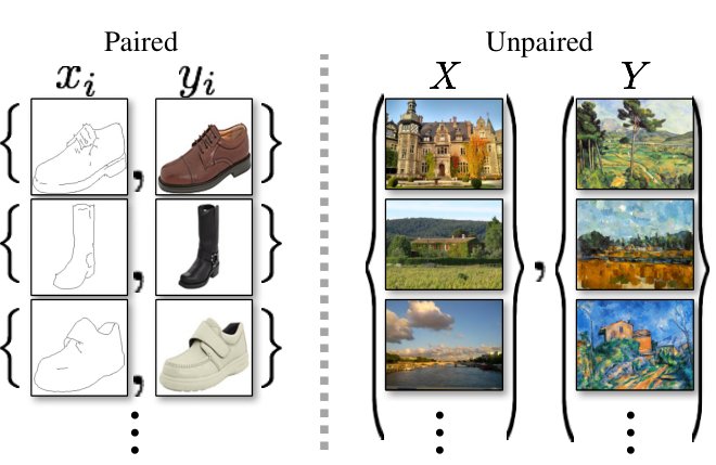
Figure 2: Paired training data (left) consists of training examples $\{x_{i},y_{i}\}_{i=1}^{N}$, where the correspondence between $x_{i}$ and $y_{i}$ exists [22]. We instead consider unpaired training data (right), consisting of a source set $\{x_{i}\}_{i=1}^{N}$ ($x_{i}\in X$) and a target set $\{y_{j}\}_{j=1}^{M}$ ($y_{j}\in Y$), with no information provided as to which $x_{i}$ matches which $y_{j}$.

图 2：配对 训练数据（左）由训练示例$\{x_{i},y_{i}\}_{i=1}^{N}$组成，其中$x_{i}$和$y_{i}$之间存在对应关系[22]。 相反，我们考虑未配对的训练数据（右），由源集$\{x_{i}\}_{i=1}^{N}$($x_{i}\in X$) 和目标集$\{y_{j}\}_{j=1}^{M}$($y_{j}\in Y$) 组成，没有提供关于哪个$x_{i}$与哪个$y_{j}$匹配的信息。

We can imagine all this despite never having seen a side by side example of a Monet painting next to a photo of the scene he painted. Instead, we have knowledge of the set of Monet paintings and of the set of landscape photographs. We can reason about the stylistic differences between these two sets, and thereby imagine what a scene might look like if we were to “translate” it from one set into the other.

尽管我们从未见过莫奈画作与他所画场景的照片并排的例子，但我们可以想象这一切。 相反，我们了解莫奈的一组画作和一组风景照片。 我们可以推断出这两组之间的风格差异，从而想象如果我们将一个场景从一组“翻译”到另一组中会是什么样子。

In this paper, we present a method that can learn to do the same: capturing special characteristics of one image collection and figuring out how these characteristics could be translated into the other image collection, all in the absence of any paired training examples.

在本文中，我们提出了一种可以学习实现相同操作的方法：捕获一个图像集合的特殊特征，并弄清楚如何将这些特征转化为另一个图像集合，所有这些都在没有任何配对训练示例的情况下进行。

This problem can be more broadly described as image-to-image translation [22], converting an image from one representation of a given scene, $x$, to another, $y$, e.g., grayscale to color, image to semantic labels, edge-map to photograph. Years of research in computer vision, image processing, computational photography, and graphics have produced powerful translation systems in the supervised setting, where example image pairs $\{x_{i},y_{i}\}_{i=1}^{N}$ are available (Figure 2, left), e.g., [11, 19, 22, 23, 28, 33, 45, 56, 58, 62]. However, obtaining paired training data can be difficult and expensive. For example, only a couple of datasets exist for tasks like semantic segmentation (e.g., [4]), and they are relatively small. Obtaining input-output pairs for graphics tasks like artistic stylization can be even more difficult since the desired output is highly complex, typically requiring artistic authoring. For many tasks, like object transfiguration (e.g., zebra$\leftrightarrow$horse,  Figure 1 top-middle), the desired output is not even well-defined.

这个问题可以更广泛地描述为图像到图像的转换[22]，将图像从给定场景的一种表示形式$x$转换为另一种表示形式$y$，例如，灰度到颜色、图像到语义标签、边缘图到照片。 计算机视觉、图像处理、计算摄影和图形方面的多年研究已经在监督环境中产生了强大的翻译系统，其中提供了示例图像对 $\{x_{i},y_{i}\}_{i=1}^{N}$（图 2，左），例如 [11, 19, 22, 23, 28, 33, 45, 56, 58, 62]。 然而，获取配对训练数据可能很困难且昂贵。 例如，只有几个数据集用于语义分割等任务（例如[4]），而且它们相对较小。 获得艺术风格化等图形任务的输入输出对可能更加困难，因为所需的输出非常复杂，通常需要艺术创作。 对于许多任务，例如对象变形（例如，斑马$\leftrightarrow$马，图 1 中上），所需的输出甚至没有明确定义。

We therefore seek an algorithm that can learn to translate between domains without paired input-output examples (Figure 2, right). We assume there is some underlying relationship between the domains – for example, that they are two different renderings of the same underlying scene – and seek to learn that relationship. Although we lack supervision in the form of paired examples, we can exploit supervision at the level of sets: we are given one set of images in domain $X$ and a different set in domain $Y$. We may train a mapping $G:X\rightarrow Y$ such that the output $\hat{y}=G(x)$, $x\in X$, is indistinguishable from images $y\in Y$ by an adversary trained to classify $\hat{y}$ apart from $y$. In theory, this objective can induce an output distribution over $\hat{y}$ that matches the empirical distribution $p_{data}(y)$ (in general, this requires $G$ to be stochastic) [16]. The optimal $G$ thereby translates the domain $X$ to a domain $\hat{Y}$ distributed identically to $Y$. However, such a translation does not guarantee that an individual input $x$ and output $y$ are paired up in a meaningful way – there are infinitely many mappings $G$ that will induce the same distribution over $\hat{y}$. Moreover, in practice, we have found it difficult to optimize the adversarial objective in isolation: standard procedures often lead to the well-known problem of mode collapse, where all input images map to the same output image and the optimization fails to make progress [15].

因此，我们寻求一种无需配对输入-输出示例即可学习在域之间进行翻译的算法（图 2，右）。 我们假设域之间存在某种潜在的关系——例如，它们是同一底层场景的两种不同的渲染——并试图学习这种关系。 尽管我们缺乏配对示例形式的监督，但我们可以利用集合级别的监督：我们在域$X$中得到一组图像，在域$Y$中得到一组不同的图像。 我们可以训练映射$G:X\rightarrow Y$，使得输出$\hat{y}=G(x)$、$x\in X$与经过训练将$\hat{y}$与$y$分类的对手无法与图像$y\in Y$区分开来。 理论上，这个目标可以在$\hat{y}$上产生与经验分布$p_{data}(y)$相匹配的输出分布（一般来说，这要求$G$是随机的）[16]。 最佳$G$从而将域$X$翻译为与$Y$分布相同的域$\hat{Y}$。 然而，这样的转换并不能保证单个输入$x$和输出$y$以有意义的方式配对 - 有无限多个映射$G$会在$\hat{y}$上产生相同的分布。 此外，在实践中，我们发现很难单独优化对抗性目标：标准程序通常会导致众所周知的模式崩溃问题，即所有输入图像映射到相同的输出图像，并且优化无法取得进展[15]。

These issues call for adding more structure to our objective. Therefore, we exploit the property that translation should be “cycle consistent”, in the sense that if we translate, e.g., a sentence from English to French, and then translate it back from French to English, we should arrive back at the original sentence [3]. Mathematically, if we have a translator $G:X\rightarrow Y$ and another translator $F:Y\rightarrow X$, then $G$ and $F$ should be inverses of each other, and both mappings should be bijections. We apply this structural assumption by training both the mapping $G$ and $F$ simultaneously, and adding a cycle consistency loss [64] that encourages $F(G(x))\approx x$ and $G(F(y))\approx y$. Combining this loss with adversarial losses on domains $X$ and $Y$ yields our full objective for unpaired image-to-image translation.

这些问题要求我们给目标加更多结构。因此我们利用翻译应“循环一致”的性质：例如把一句英文译成法文再译回英文，应回到原句。在图像上，若有映射 $G:X\to Y$ 与 $F:Y\to X$，则 $G$、$F$ 应互为逆，且两映射都应是双射。我们用循环一致性损失从数值上激励这种行为。

We apply our method to a wide range of applications, including collection style transfer, object transfiguration, season transfer and photo enhancement. We also compare against previous approaches that rely either on hand-defined factorizations of style and content, or on shared embedding functions, and show that our method outperforms these baselines. We provide both PyTorch and Torch implementations. Check out more results at our website.

我们将我们的方法应用于广泛的应用，包括收藏风格转移、对象变形、季节转移和照片增强。 我们还与以前依赖于手动定义的样式和内容分解或共享嵌入函数的方法进行比较，并表明我们的方法优于这些基线。 我们提供 PyTorch 和 Torch 实现。 在我们的网站上查看更多结果。

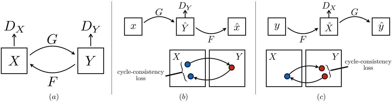
Figure 3: (a) Our model contains two mapping functions $G:X\rightarrow Y$ and $F:Y\rightarrow X$, and associated adversarial discriminators $D_{Y}$ and $D_{X}$. $D_{Y}$ encourages $G$ to translate $X$ into outputs indistinguishable from domain $Y$, and vice versa for $D_{X}$ and $F$. To further regularize the mappings, we introduce two cycle consistency losses that capture the intuition that if we translate from one domain to the other and back again we should arrive at where we started: (b) forward cycle-consistency loss: $x\rightarrow G(x)\rightarrow F(G(x))\approx x$, and (c) backward cycle-consistency loss: $y\rightarrow F(y)\rightarrow G(F(y))\approx y$

图 3：(a) 我们的模型包含两个映射函数$G:X\rightarrow Y$和$F:Y\rightarrow X$，以及相关的对抗性判别器$D_{Y}$和$D_{X}$。$D_{Y}$鼓励$G$将$X$转换为与域$Y$无法区分的输出，对于$D_{X}$和$F$反之亦然。 为了进一步规范映射，我们引入了两个“循环一致性损失”，它们捕捉了这样的直觉：如果我们从一个域转换到另一个域并再次返回，我们应该到达我们开始的地方：（b）前向循环一致性损失：$x\rightarrow G(x)\rightarrow F(G(x))\approx x$，以及（c）后向循环一致性损失：$y\rightarrow F(y)\rightarrow G(F(y))\approx y$

2 Related work

2 相关工作

Generative Adversarial Networks (GANs) [16, 63] have achieved impressive results in image generation [6, 39], image editing [66], and representation learning [39, 43, 37].　 Recent methods adopt the same idea for conditional image generation applications, such as text2image [41], image inpainting [38], and future prediction [36], as well as to other domains like videos [54] and 3D data [57]. The key to GANs’ success is the idea of an adversarial loss that forces the generated images to be, in principle, indistinguishable from real photos. This loss is particularly powerful for image generation tasks, as this is exactly the objective that much of computer graphics aims to optimize. We adopt an adversarial loss to learn the mapping such that the translated images cannot be distinguished from images in the target domain.

生成对抗网络 (GAN) [16, 63] 在图像生成 [6, 39]、图像编辑 [66] 和表示学习 [39, 43, 37] 方面取得了令人印象深刻的成果。 最近的方法在条件图像生成应用程序中采用了相同的想法，例如文本2图像[41]、图像修复[38]和未来预测[36]，以及视频[54]和3D数据[57]等其他领域。 GAN 成功的关键是“对抗性损失”的想法，它迫使生成的图像原则上与真实照片无法区分。 这种损失对于图像生成任务尤其严重，因为这正是许多计算机图形学旨在优化的目标。 我们采用对抗性损失来学习映射，使得翻译后的图像无法与目标域中的图像区分开。

Image-to-Image Translation The idea of image-to-image translation goes back at least to Hertzmann et al.’s Image Analogies [19], who employ a non-parametric texture model [10] on a single input-output training image pair. More recent approaches use a dataset of input-output examples to learn a parametric translation function using CNNs (e.g., [33]). Our approach builds on the “pix2pix” framework of Isola et al. [22], which uses a conditional generative adversarial network [16] to learn a mapping from input to output images. Similar ideas have been applied to various tasks such as generating photographs from sketches [44] or from attribute and semantic layouts [25]. However, unlike the above prior work, we learn the mapping without paired training examples.

图像到图像转换 图像到图像转换的想法至少可以追溯到 Hertzmann 等人的图像类比 [19]，他们在单个输入-输出训练图像对上采用非参数纹理模型 [10]。 最近的方法使用输入输出示例的“数据集”来学习使用 CNN 的参数翻译函数（例如，[33]）。 我们的方法建立在 Isola 等人的“pix2pix”框架之上。 [22]，它使用条件生成对抗网络[16]来学习从输入到输出图像的映射。 类似的想法已应用于各种任务，例如从草图 [44] 或从属性和语义布局 [25] 生成照片。 然而，与上述先前的工作不同，我们在没有配对训练示例的情况下学习映射。

Unpaired Image-to-Image Translation Several other methods also tackle the unpaired setting, where the goal is to relate two data domains: $X$ and $Y$. Rosales et al. [42] propose a Bayesian framework that includes a prior based on a patch-based Markov random field computed from a source image and a likelihood term obtained from multiple style images. More recently, CoGAN [32] and cross-modal scene networks [1] use a weight-sharing strategy to learn a common representation across domains. Concurrent to our method, Liu et al. [31] extends the above framework with a combination of variational autoencoders [27] and generative adversarial networks [16]. Another line of concurrent work [46, 49, 2] encourages the input and output to share specific “content” features even though they may differ in “style“. These methods also use adversarial networks, with additional terms to enforce the output to be close to the input in a predefined metric space, such as class label space [2], image pixel space [46], and image feature space [49].

不成对的图像到图像转换 其他几种方法也可以解决不成对的设置，其目标是关联两个数据域：$X$和$Y$。 罗萨莱斯等人。 [42]提出了一个贝叶斯框架，其中包括基于从源图像计算的基于补丁的马尔可夫随机场的先验和从多个风格图像获得的似然项。 最近，CoGAN [32] 和跨模态场景网络 [1] 使用权重共享策略来学习跨领域的通用表示。 与我们的方法同时，刘等人。 [31]通过变分自动编码器[27]和生成对抗网络[16]的组合扩展了上述框架。 另一条并行工作[46,49,2]鼓励输入和输出共享特定的“内容”功能，即使它们的“风格”可能不同。 这些方法还使用对抗网络，并使用附加项来强制输出接近预定义度量空间中的输入，例如类标签空间 [2]、图像像素空间 [46] 和图像特征空间 [49]。

Unlike the above approaches, our formulation does not rely on any task-specific, predefined similarity function between the input and output, nor do we assume that the input and output have to lie in the same low-dimensional embedding space. This makes our method a general-purpose solution for many vision and graphics tasks. We directly compare against several prior and contemporary approaches in Section 5.1.

与上述方法不同，我们的公式不依赖于输入和输出之间任何特定于任务的预定义相似性函数，也不假设输入和输出必须位于相同的低维嵌入空间中。 这使得我们的方法成为许多视觉和图形任务的通用解决方案。 我们在第 5.1 节中直接与几种先前和当代的方法进行比较。

Cycle Consistency The idea of using transitivity as a way to regularize structured data has a long history. In visual tracking, enforcing simple forward-backward consistency has been a standard trick for decades [24, 48]. In the language domain, verifying and improving translations via “back translation and reconciliation” is a technique used by human translators [3] (including, humorously, by Mark Twain [51]), as well as by machines [17]. More recently, higher-order cycle consistency has been used in structure from motion [61], 3D shape matching [21], co-segmentation [55], dense semantic alignment [65, 64], and depth estimation [14]. Of these, Zhou et al. [64] and Godard et al. [14] are most similar to our work, as they use a cycle consistency loss as a way of using transitivity to supervise CNN training. In this work, we are introducing a similar loss to push $G$ and $F$ to be consistent with each other. Concurrent with our work, in these same proceedings, Yi et al. [59] independently use a similar objective for unpaired image-to-image translation, inspired by dual learning in machine translation [17].

循环一致性 使用传递性作为规范结构化数据的方法的想法有着悠久的历史。 在视觉跟踪中，几十年来，强制实现简单的前后一致性一直是标准技巧 [24, 48]。 在语言领域，通过“反向翻译和协调”验证和改进翻译是人类翻译人员 [3]（幽默地包括马克·吐温 [51]）以及机器 [17] 使用的技术。 最近，高阶循环一致性已被用于运动结构[61]、3D形状匹配[21]、共同分割[55]、密集语义对齐[65, 64]和深度估计[14]。 其中，周等人。 [64]和戈达尔等人。 [14] 与我们的工作最相似，因为他们使用“循环一致性损失”作为使用传递性来监督 CNN 训练的一种方式。 在这项工作中，我们引入了类似的损失来推动$G$和$F$彼此一致。 与我们的工作同时，在这些相同的程序中，Yi 等人。 [59] 受到机器翻译中对偶学习的启发，独立使用类似的目标进行不配对的图像到图像的翻译 [17]。

Neural Style Transfer [13, 23, 52, 12] is another way to perform image-to-image translation, which synthesizes a novel image by combining the content of one image with the style of another image (typically a painting) based on matching the Gram matrix statistics of pre-trained deep features. Our primary focus, on the other hand, is learning the mapping between two image collections, rather than between two specific images, by trying to capture correspondences between higher-level appearance structures. Therefore, our method can be applied to other tasks, such as painting$\rightarrow$ photo, object transfiguration, etc. where single sample transfer methods do not perform well. We compare these two methods in  Section 5.2.

神经风格迁移 [13,23,52,12]是实现图像到图像转换的另一种方法，它根据匹配预训练深度特征的 Gram 矩阵统计数据，通过将一个图像的内容与另一个图像（通常是绘画）的风格相结合来合成新颖的图像。 另一方面，我们的主要重点是通过尝试捕获更高级别的外观结构之间的对应关系来学习两个图像集合之间的映射，而不是两个特定图像之间的映射。 因此，我们的方法可以应用于其他任务，例如绘制$\rightarrow$照片、对象变形等单样本传输方法表现不佳的任务。 我们在第 5.2 节中比较了这两种方法。

3 Formulation

3 形式化

Our goal is to learn mapping functions between two domains $X$ and $Y$ given training samples $\{x_{i}\}_{i=1}^{N}$ where $x_{i}\in X$ and $\{y_{j}\}_{j=1}^{M}$ where $y_{j}\in Y$[^1]. We denote the data distribution as $x\sim p_{data}(x)$ and $y\sim p_{data}(y)$. As illustrated in Figure 3 (a), our model includes two mappings $G:X\rightarrow Y$ and $F:Y\rightarrow X$. In addition, we introduce two adversarial discriminators $D_{X}$ and $D_{Y}$, where $D_{X}$ aims to distinguish between images $\{x\}$ and translated images $\{F(y)\}$; in the same way, $D_{Y}$ aims to discriminate between $\{y\}$ and $\{G(x)\}$. Our objective contains two types of terms: adversarial losses [16] for matching the distribution of generated images to the data distribution in the target domain; and cycle consistency losses to prevent the learned mappings $G$ and $F$ from contradicting each other.

我们的目标是在给定训练样本 $\{x_{i}\}_{i=1}^{N}$（其中$x_{i}\in X$和 $\{y_{j}\}_{j=1}^{M}$（其中$y_{j}\in Y$[^1]））的情况下学习两个域$X$和$Y$之间的映射函数。 我们将数据分布表示为$x\sim p_{data}(x)$和$y\sim p_{data}(y)$。 如图 3 (a) 所示，我们的模型包括两个映射$G:X\rightarrow Y$和$F:Y\rightarrow X$。 此外，我们引入了两个对抗性判别器$D_{X}$和$D_{Y}$，其中$D_{X}$旨在区分图像$\{x\}$和翻译图像$\{F(y)\}$； 同样，$D_{Y}$的目的是区分$\{y\}$和$\{G(x)\}$。 我们的目标包含两种类型的术语：对抗性损失[16]，用于将生成的图像的分布与目标域中的数据分布进行匹配； 和循环一致性损失，以防止学习到的映射$G$和$F$相互矛盾。

3.1 Adversarial Loss

3.1 对抗损失

We apply adversarial losses [16] to both mapping functions. For the mapping function $G:X\rightarrow Y$ and its discriminator $D_{Y}$, we express the objective as:

我们将对抗性损失[16]应用于两个映射函数。 对于映射函数$G:X\rightarrow Y$及其判别器$D_{Y}$，我们将目标表示为：

$$\displaystyle\mathcal{L}_{\text{GAN}}(G,D_{Y},X,Y)= \\ \displaystyle\ \mathbb{E}_{y\sim p_{\text{data}}(y)}[\log D_{Y}(y)] \\ \displaystyle+ \\ \displaystyle\ \mathbb{E}_{x\sim p_{\text{data}}(x)}[\log(1-D_{Y}(G(x))], \tag{1}$$

where $G$ tries to generate images $G(x)$ that look similar to images from domain $Y$, while $D_{Y}$ aims to distinguish between translated samples $G(x)$ and real samples $y$. $G$ aims to minimize this objective against an adversary $D$ that tries to maximize it, i.e., $\min_{G}\max_{D_{Y}}\mathcal{L}_{\text{GAN}}(G,D_{Y},X,Y)$. We introduce a similar adversarial loss for the mapping function $F:Y\rightarrow X$ and its discriminator $D_{X}$ as well: i.e., $\min_{F}\max_{D_{X}}\mathcal{L}_{\text{GAN}}(F,D_{X},Y,X)$.

其中$G$尝试生成与域$Y$中的图像相似的图像$G(x)$，而$D_{Y}$旨在区分翻译样本$G(x)$和真实样本$y$。$G$的目标是最小化这一目标，而对手$D$则试图最大化该目标，即$\min_{G}\max_{D_{Y}}\mathcal{L}_{\text{GAN}}(G,D_{Y},X,Y)$。 我们还为映射函数$F:Y\rightarrow X$及其鉴别器$D_{X}$引入了类似的对抗性损失：即$\min_{F}\max_{D_{X}}\mathcal{L}_{\text{GAN}}(F,D_{X},Y,X)$。

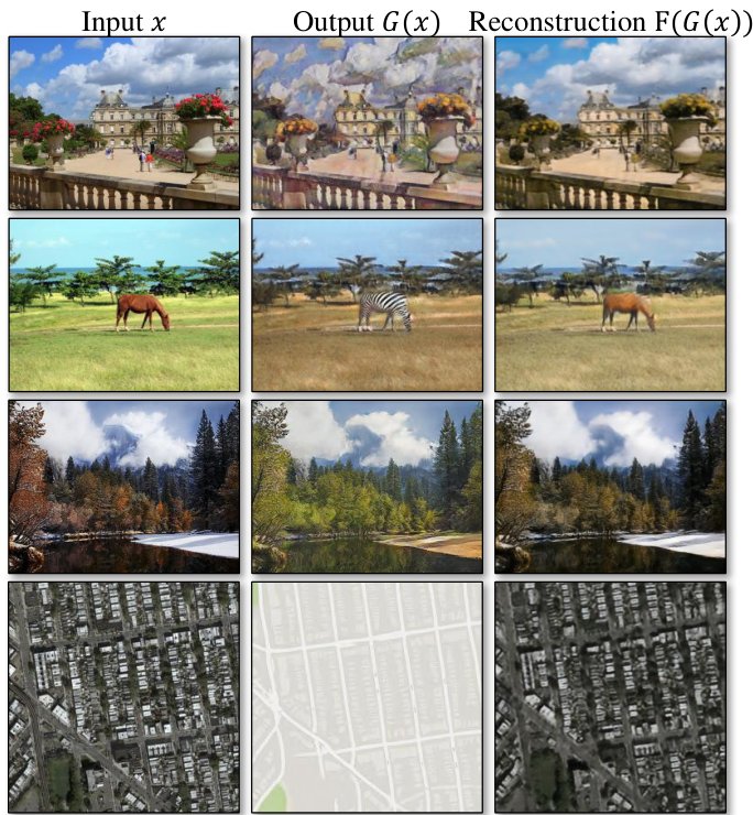
Figure 4: The input images $x$, output images $G(x)$ and the reconstructed images $F(G(x))$ from various experiments. From top to bottom: photo$\leftrightarrow$Cezanne, horses$\leftrightarrow$zebras, winter$\rightarrow$summer Yosemite, aerial photos$\leftrightarrow$Google maps.

图 4：来自各种实验的输入图像$x$、输出图像$G(x)$和重建图像$F(G(x))$。 从上到下：照片$\leftrightarrow$塞尚、马$\leftrightarrow$斑马、冬季$\rightarrow$夏季优胜美地、航拍照片$\leftrightarrow$谷歌地图。

3.2 Cycle Consistency Loss

3.2 循环一致性损失

Adversarial training can, in theory, learn mappings $G$ and $F$ that produce outputs identically distributed as target domains $Y$ and $X$ respectively (strictly speaking, this requires $G$ and $F$ to be stochastic functions) [15]. However, with large enough capacity, a network can map the same set of input images to any random permutation of images in the target domain, where any of the learned mappings can induce an output distribution that matches the target distribution. Thus, adversarial losses alone cannot guarantee that the learned function can map an individual input $x_{i}$ to a desired output $y_{i}$. To further reduce the space of possible mapping functions, we argue that the learned mapping functions should be cycle-consistent: as shown in Figure 3 (b), for each image $x$ from domain $X$, the image translation cycle should be able to bring $x$ back to the original image, i.e., $x\rightarrow G(x)\rightarrow F(G(x))\approx x$. We call this forward cycle consistency. Similarly, as illustrated in Figure 3 (c), for each image $y$ from domain $Y$, $G$ and $F$ should also satisfy backward cycle consistency: $y\rightarrow F(y)\rightarrow G(F(y))\approx y$. We incentivize this behavior using a cycle consistency loss:

理论上，对抗训练可以学习映射$G$和 $F$，分别产生与目标域$Y$和$X$相同分布的输出（严格来说，这要求$G$和$F$是随机函数）[15]。 然而，如果容量足够大，网络可以将同一组输入图像映射到目标域中图像的任意随机排列，其中任何学习到的映射都可以得出与目标分布匹配的输出分布。 因此，仅对抗性损失不能保证学习的函数可以将单个输入$x_{i}$映射到所需的输出$y_{i}$。 为了进一步减少可能的映射函数的空间，我们认为学习的映射函数应该是循环一致的：如图 3 (b) 所示，对于来自域$X$的每个图像$x$，图像转换循环应该能够将$x$返回到原始图像，即$x\rightarrow G(x)\rightarrow F(G(x))\approx x$。 我们称之为“前向循环一致性”。 类似地，如图 3 (c) 所示，对于来自域$Y$、$G$和$F$的每个图像$y$也应满足后向循环一致性：$y\rightarrow F(y)\rightarrow G(F(y))\approx y$ 。 我们使用循环一致性损失来激励这种行为：

$$\displaystyle\mathcal{L}_{\text{cyc}}(G,F)= \\ \displaystyle\ \mathbb{E}_{x\sim p_{\text{data}}(x)}[\lVert F(G(x))-x\rVert_{1}] \\ \displaystyle+ \\ \displaystyle\ \mathbb{E}_{y\sim p_{\text{data}}(y)}[\lVert G(F(y))-y\rVert_{1}]. \tag{2}$$

In preliminary experiments, we also tried replacing the L1 norm in this loss with an adversarial loss between $F(G(x))$ and $x$, and between $G(F(y))$ and $y$, but did not observe improved performance.

在初步实验中，我们还尝试用$F(G(x))$和$x$之间以及$G(F(y))$和$y$之间的对抗性损失替换该损失中的 L1 范数，但没有观察到性能的提高。

The behavior induced by the cycle consistency loss can be observed in Figure 4: the reconstructed images $F(G(x))$ end up matching closely to the input images $x$.

由循环一致性损失引起的行为可以在图 4 中观察到：重建图像$F(G(x))$最终与输入图像$x$紧密匹配。

3.3 Full Objective

3.3 完整目标

Our full objective is:

我们的全部目标是：

$$\displaystyle\mathcal{L}(G,F,D_{X},D_{Y})= \\ \displaystyle、\mathcal{L}_{\text{GAN}}(G,D_{Y},X,Y) \\ \displaystyle+ \\ \displaystyle\ \mathcal{L}_{\text{GAN}}(F,D_{X},Y,X) \\ \displaystyle+ \\ \displaystyle\ \lambda\mathcal{L}_{\text{cyc}}(G,F), \tag{3}$$

where $\lambda$ controls the relative importance of the two objectives. We aim to solve:

其中$\lambda$控制两个目标的相对重要性。 我们的目标是解决：

$$G^{*},F^{*}=\arg\min_{G,F}\max_{D_{x},D_{Y}}\mathcal{L}(G,F,D_{X},D_{Y}). \tag{4}$$

Notice that our model can be viewed as training two “autoencoders” [20]: we learn one autoencoder $F\circ G:X\rightarrow X$ jointly with another $G\circ F:Y\rightarrow Y$. However, these autoencoders each have special internal structures: they map an image to itself via an intermediate representation that is a translation of the image into another domain. Such a setup can also be seen as a special case of “adversarial autoencoders” [34], which use an adversarial loss to train the bottleneck layer of an autoencoder to match an arbitrary target distribution. In our case, the target distribution for the $X\rightarrow X$ autoencoder is that of the domain $Y$.

请注意，我们的模型可以被视为训练两个“自动编码器”[20]：我们联合学习一个自动编码器$F\circ G:X\rightarrow X$和另一个$G\circ F:Y\rightarrow Y$。 然而，这些自动编码器都有特殊的内部结构：它们通过中间表示将图像映射到自身，中间表示是将图像转换为另一个域。 这种设置也可以被视为“对抗性自动编码器”的特殊情况[34]，它使用对抗性损失来训练自动编码器的瓶颈层以匹配任意目标分布。 在我们的例子中，$X\rightarrow X$自动编码器的目标分布是域$Y$的目标分布。

In Section 5.1.4, we compare our method against ablations of the full objective, including the adversarial loss $\mathcal{L}_{\text{GAN}}$ alone and the cycle consistency loss $\mathcal{L}_{\text{cyc}}$ alone, and empirically show that both objectives play critical roles in arriving at high-quality results. We also evaluate our method with only cycle loss in one direction and show that a single cycle is not sufficient to regularize the training for this under-constrained problem.

在第 5.1.4 节中，我们将我们的方法与完整目标的消融进行比较，包括单独的对抗性损失$\mathcal{L}_{\text{GAN}}$和单独的循环一致性损失 $\mathcal{L}_{\text{cyc}}$，并凭经验表明这两个目标在获得高质量结果方面都发挥着关键作用。 我们还评估了我们的方法，仅在一个方向上存在循环损失，并表明单个循环不足以规范这一欠约束问题的训练。

4 Implementation

4 实现

Network Architecture

We adopt the architecture for our generative networks from Johnson et al. [23] who have shown impressive results for neural style transfer and super-resolution. This network contains three convolutions, several residual blocks [18], two fractionally-strided convolutions with stride $\frac{1}{2}$, and one convolution that maps features to RGB. We use $6$ blocks for $128\times 128$ images and $9$ blocks for $256\times 256$ and higher-resolution training images. Similar to Johnson et al. [23], we use instance normalization [53]. For the discriminator networks we use $70\times 70$ PatchGANs [22, 30, 29], which aim to classify whether $70\times 70$ overlapping image patches are real or fake. Such a patch-level discriminator architecture has fewer parameters than a full-image discriminator and can work on arbitrarily-sized images in a fully convolutional fashion [22].

网络架构

我们采用 Johnson 等人的生成网络架构。 [23] 在神经风格迁移和超分辨率方面取得了令人印象深刻的成果。 该网络包含三个卷积、几个残差块[18]、两个步长为$\frac{1}{2}$的分数步长卷积，以及一个将特征映射到 RGB 的卷积。 我们对$128\times 128$图像使用$6$块，对$256\times 256$和更高分辨率的训练图像使用$9$块。 与约翰逊等人类似。 [23]，我们使用实例标准化[53]。 对于鉴别器网络，我们使用$70\times 70$PatchGAN [22,30,29]，其目的是对$70\times 70$重叠图像块是真还是假进行分类。 这种补丁级鉴别器架构比全图像鉴别器具有更少的参数，并且可以以完全卷积的方式处理任意大小的图像[22]。

Training details

We apply two techniques from recent works to stabilize our model training procedure. First, for $\mathcal{L}_{\text{GAN}}$ (Equation 1), we replace the negative log likelihood objective by a least-squares loss [35]. This loss is more stable during training and generates higher quality results. In particular, for a GAN loss $\mathcal{L}_{\text{GAN}}(G,D,X,Y)$, we train the $G$ to minimize $\mathbb{E}_{x\sim p_{\text{data}}(x)}[(D(G(x))-1)^{2}]$ and train the $D$ to minimize $\mathbb{E}_{y\sim p_{\text{data}}(y)}[(D(y)-1)^{2}]+\mathbb{E}_{x\sim p_{\text{data}}(x)}[D(G(x))^{2}]$.

培训详情

我们应用最近工作中的两种技术来稳定我们的模型训练过程。 首先，对于 $\mathcal{L}_{\text{GAN}}$（方程 1），我们用最小二乘损失替换负对数似然目标 [35]。 这种损失在训练过程中更加稳定，并产生更高质量的结果。 特别是，对于 GAN 损失$\mathcal{L}_{\text{GAN}}(G,D,X,Y)$，我们训练$G$以最小化$\mathbb{E}_{x\sim p_{\text{data}}(x)}[(D(G(x))-1)^{2}]$并训练$D$以最小化$\mathbb{E}_{y\sim p_{\text{data}}(y)}[(D(y)-1)^{2}]+\mathbb{E}_{x\sim p_{\text{data}}(x)}[D(G(x))^{2}]$。

Second, to reduce model oscillation [15], we follow Shrivastava et al.’s strategy [46] and update the discriminators using a history of generated images rather than the ones produced by the latest generators. We keep an image buffer that stores the $50$ previously created images.

其次，为了减少模型振荡[15]，我们遵循 Shrivastava 等人的策略[46]，并使用生成图像的历史记录而不是最新生成器生成的图像来更新鉴别器。 我们保留一个图像缓冲区来存储先前创建的$50$图像。

For all the experiments, we set $\lambda=10$ in Equation 3. We use the Adam solver [26] with a batch size of $1$. All networks were trained from scratch with a learning rate of $0.0002$. We keep the same learning rate for the first $100$ epochs and linearly decay the rate to zero over the next $100$ epochs. Please see the appendix (Section 7) for more details about the datasets, architectures, and training procedures.

对于所有实验，我们在方程 3 中设置 $\lambda=10$。我们使用 Adam 求解器 [26]，批量大小为$1$。 所有网络均以$0.0002$的学习率从头开始训练。 我们在前$100$时期保持相同的学习率，并在接下来的$100$时期将学习率线性衰减到零。 有关数据集、架构和训练程序的更多详细信息，请参阅附录（第 7 节）。

5 Results

5 结果

We first compare our approach against recent methods for unpaired image-to-image translation on paired datasets where ground truth input-output pairs are available for evaluation. We then study the importance of both the adversarial loss and the cycle consistency loss and compare our full method against several variants. Finally, we demonstrate the generality of our algorithm on a wide range of applications where paired data does not exist. For brevity, we refer to our method as CycleGAN. The PyTorch and Torch code, models, and full results can be found at our website.

我们首先将我们的方法与最近在配对数据集上进行不配对图像到图像转换的方法进行比较，其中真值标注输入输出对可用于评估。 然后，我们研究对抗性损失和循环一致性损失的重要性，并将我们的完整方法与几种变体进行比较。 最后，我们在不存在配对数据的广泛应用中证明了我们的算法的通用性。 为简洁起见，我们将我们的方法称为 CycleGAN。 PyTorch 和 Torch 代码、模型和完整结果可以在我们的网站上找到。

5.1 Evaluation

5.1 评估

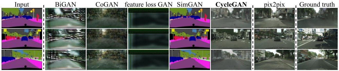
Figure 5: Different methods for mapping labels$\leftrightarrow$photos trained on Cityscapes images. From left to right: input, BiGAN/ALI [7, 9], CoGAN [32], feature loss + GAN, SimGAN [46], CycleGAN (ours), pix2pix [22] trained on paired data, and ground truth.

图 5：在城市景观图像上训练的映射标签$\leftrightarrow$照片的不同方法。 从左到右：输入、BiGAN/ALI [7, 9]、CoGAN [32]、特征损失 + GAN、SimGAN [46]、CycleGAN（我们的）、基于配对数据训练的 pix2pix [22] 和真实数据。

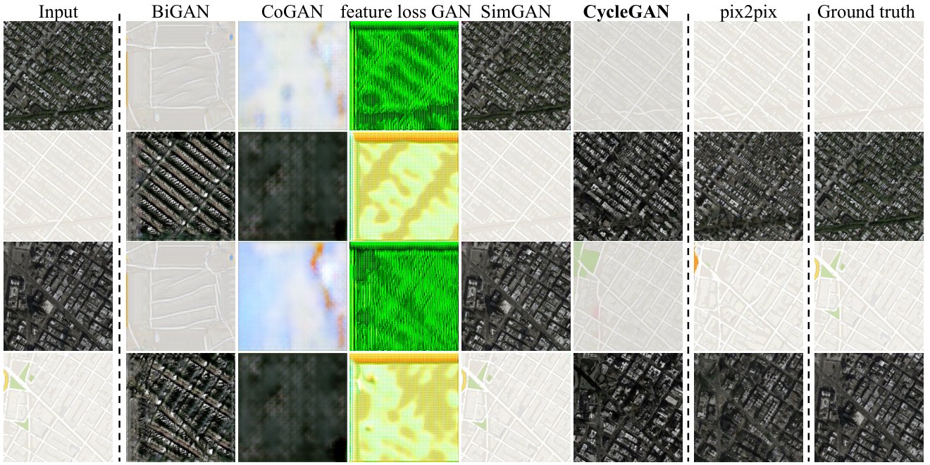
Figure 6: Different methods for mapping aerial photos$\leftrightarrow$maps on Google Maps. From left to right: input, BiGAN/ALI [7, 9], CoGAN [32], feature loss + GAN, SimGAN [46], CycleGAN (ours), pix2pix [22] trained on paired data, and ground truth.

图 6：在 Google 地图上绘制航空照片$\leftrightarrow$地图的不同方法。 从左到右：输入、BiGAN/ALI [7, 9]、CoGAN [32]、特征损失 + GAN、SimGAN [46]、CycleGAN（我们的）、基于配对数据训练的 pix2pix [22] 和真实数据。

Using the same evaluation datasets and metrics as “pix2pix” [22], we compare our method against several baselines both qualitatively and quantitatively. The tasks include semantic labels$\leftrightarrow$photo on the Cityscapes dataset [4], and map$\leftrightarrow$aerial photo on data scraped from Google Maps. We also perform ablation study on the full loss function.

使用与“pix2pix”[22]相同的评估数据集和指标，我们将我们的方法与几个基线进行定性和定量比较。 这些任务包括 Cityscapes 数据集 [4] 上的语义标签$\leftrightarrow$照片，以及根据从 Google 地图抓取的数据绘制$\leftrightarrow$航空照片。 我们还对完整的损失函数进行了消融研究。

5.1.1 Evaluation Metrics

AMT perceptual studies On the map$\leftrightarrow$aerial photo task, we run “real vs fake” perceptual studies on Amazon Mechanical Turk (AMT) to assess the realism of our outputs. We follow the same perceptual study protocol from Isola et al. [22], except we only gather data from $25$ participants per algorithm we tested. Participants were shown a sequence of pairs of images, one a real photo or map and one fake (generated by our algorithm or a baseline), and asked to click on the image they thought was real. The first $10$ trials of each session were practice and feedback was given as to whether the participant’s response was correct or incorrect. The remaining $40$ trials were used to assess the rate at which each algorithm fooled participants. Each session only tested a single algorithm, and participants were only allowed to complete a single session. The numbers we report here are not directly comparable to those in [22] as our ground truth images were processed slightly differently [^2] and the participant pool we tested may be differently distributed from those tested in [22] (due to running the experiment at a different date and time). Therefore, our numbers should only be used to compare our current method against the baselines (which were run under identical conditions), rather than against [22].

5.1.1 评估指标

AMT 感知研究 在地图$\leftrightarrow$航空照片任务中，我们在 Amazon Mechanical Turk (AMT) 上运行“真与假”感知研究，以评估我们输出的真实性。 我们遵循 Isola 等人的相同感知研究方案。 [22]，除了我们只根据我们测试的算法收集$25$参与者的数据。 向参与者展示了一系列图像对，其中一幅是真实的照片或地图，一幅是假的（由我们的算法或基线生成），并要求他们点击他们认为真实的图像。 每节的第一次$10$试验都是练习，并就参与者的反应是否正确给出反馈。 其余的$40$试验用于评估每种算法愚弄参与者的比率。 每个会话仅测试一个算法，并且参与者仅被允许完成一个会话。 我们在此报告的数字不能直接与 [22] 中的数据进行比较，因为我们的真值标注图像的处理方式略有不同 [^2]，并且我们测试的参与者池的分布可能与 [22] 中测试的参与者池的分布不同（由于在不同的日期和时间运行实验）。 因此，我们的数字只能用于将我们当前的方法与基线（在相同条件下运行）进行比较，而不是与[22]进行比较。

FCN score Although perceptual studies may be the gold standard for assessing graphical realism, we also seek an automatic quantitative measure that does not require human experiments. For this, we adopt the “FCN score” from [22], and use it to evaluate the Cityscapes labels$\rightarrow$photo task. The FCN metric evaluates how interpretable the generated photos are according to an off-the-shelf semantic segmentation algorithm (the fully-convolutional network, FCN, from [33]). The FCN predicts a label map for a generated photo. This label map can then be compared against the input ground truth labels using standard semantic segmentation metrics described below. The intuition is that if we generate a photo from a label map of “car on the road”, then we have succeeded if the FCN applied to the generated photo detects “car on the road”.

FCN 分数 虽然感知研究可能是评估图形真实性的黄金标准，但我们还寻求一种不需要人体实验的自动定量测量。 为此，我们采用[22]中的“FCN 分数”，并用它来评估 Cityscapes 标签$\rightarrow$照片任务。 FCN 指标根据现成的语义分割算法（全卷积网络 FCN，来自 [33]）评估生成的照片的可解释性。 FCN 预测生成照片的标签图。 然后可以使用下面描述的标准语义分割指标将该标签图与输入的地面真实标签进行比较。 直觉是，如果我们从“路上的汽车”标签图生成一张照片，那么如果应用于生成的照片的 FCN 检测到“路上的汽车”，我们就成功了。

Semantic segmentation metrics To evaluate the performance of photo$\rightarrow$labels, we use the standard metrics from the Cityscapes benchmark [4], including per-pixel accuracy, per-class accuracy, and mean class Intersection-Over-Union (Class IOU) [4].

语义分割指标 为了评估照片$\rightarrow$标签的性能，我们使用 Cityscapes 基准 [4] 中的标准指标，包括每像素精度、每类精度和平均类 Intersection-Over-Union（IOU 类）[4]。

5.1.2 Baselines

CoGAN [32] This method learns one GAN generator for domain $X$ and one for domain $Y$, with tied weights on the first few layers for shared latent representations. Translation from $X$ to $Y$ can be achieved by finding a latent representation that generates image $X$ and then rendering this latent representation into style $Y$.

5.1.2 基线

CoGAN [32] 该方法学习一个用于域$X$的 GAN 生成器和一个用于域$Y$的 GAN 生成器，并在前几层上绑定权重以实现共享潜在表示。 从$X$到$Y$的转换可以通过找到生成图像$X$的潜在表示，然后将该潜在表示渲染为样式$Y$来实现。

SimGAN [46] Like our method, Shrivastava et al.[46] uses an adversarial loss to train a translation from $X$ to $Y$. The regularization term $\lVert x-G(x)\rVert_{1}$ i s used to penalize making large changes at pixel level.

SimGAN [46] 就像我们的方法一样，Shrivastava 等人[46] 使用对抗性损失来训练从$X$到$Y$的翻译。 正则化项$\lVert x-G(x)\rVert_{1}$用于惩罚在像素级别进行较大更改。

Feature loss + GAN We also test a variant of SimGAN [46] where the L1 loss is computed over deep image features using a pretrained network (VGG-16 relu4_2 [47]), rather than over RGB pixel values. Computing distances in deep feature space, like this, is also sometimes referred to as using a “perceptual loss” [8, 23].

特征损失 + GAN 我们还测试了 SimGAN [46] 的一个变体，其中 L1 损失是使用预训练网络 (VGG-16 relu4_2 [47]) 根据深度图像特征计算的，而不是根据 RGB 像素值计算的。 像这样计算深层特征空间中的距离有时也称为使用“感知损失”[8, 23]。

BiGAN/ALI [9, 7] Unconditional GANs [16] learn a generator $G:Z\rightarrow X$, that maps a random noise $z$ to an image $x$. The BiGAN [9] and ALI [7] propose to also learn the inverse mapping function $F:X\rightarrow Z$. Though they were originally designed for mapping a latent vector $z$ to an image $x$, we implemented the same objective for mapping a source image $x$ to a target image $y$.

BiGAN/ALI [9, 7] 无条件 GAN [16] 学习生成器$G:Z\rightarrow X$，它将随机噪声$z$映射到图像$x$。 BiGAN [9] 和 ALI [7] 建议还学习逆映射函数$F:X\rightarrow Z$。 虽然它们最初设计用于将潜在向量$z$映射到图像$x$，但我们实现了相同的目标，将源图像$x$映射到目标图像$y$。

pix2pix [22] We also compare against pix2pix [22], which is trained on paired data, to see how close we can get to this “upper bound” without using any paired data.

pix2pix [22] 我们还与在配对数据上进行训练的 pix2pix [22] 进行比较，看看我们在不使用任何配对数据的情况下能够接近这个“上限”。

For a fair comparison, we implement all the baselines using the same architecture and details as our method, except for CoGAN [32]. CoGAN builds on generators that produce images from a shared latent representation, which is incompatible with our image-to-image network. We use the public implementation of CoGAN instead.

为了公平比较，我们使用与我们的方法相同的架构和细节来实现所有基线，CoGAN [32] 除外。 CoGAN 建立在从共享潜在表示生成图像的生成器之上，这与我们的图像到图像网络不兼容。 我们改用 CoGAN 的公共实现。

	Map $\rightarrow$ Photo	Photo $\rightarrow$ Map
Loss	% Turkers labeled real	% Turkers labeled real
CoGAN [32]	0.6% $\pm$ 0.5%	0.9% $\pm$ 0.5%
BiGAN/ALI [9, 7]	2.1% $\pm$ 1.0%	1.9% $\pm$ 0.9%
SimGAN [46]	0.7% $\pm$ 0.5%	2.6% $\pm$ 1.1%
Feature loss + GAN	1.2% $\pm$ 0.6%	0.3% $\pm$ 0.2%
CycleGAN (ours)	26.8% $\pm$ 2.8%	23.2% $\pm$ 3.4%

Table 1: AMT “real vs fake” test on maps$\leftrightarrow$aerial photos at $256\times 256$ resolution.

	地图$\rightarrow$照片	照片$\rightarrow$地图
损失	被标记为真实的土耳其人百分比	被标记为真实的土耳其人百分比
CoGAN [32]	0.6% $\pm$ 0.5%	0.9% $\pm$ 0.5%
BiGAN/ALI [9, 7]	2.1% $\pm$ 1.0%	1.9% $\pm$ 0.9%
SimGAN [46]	0.7% $\pm$ 0.5%	2.6% $\pm$ 1.1%
特征损失+GAN	1.2% $\pm$ 0.6%	0.3% $\pm$ 0.2%
CycleGAN（我们的）	26.8% $\pm$ 2.8%	23.2% $\pm$ 3.4%

表 1：在$256\times 256$分辨率的地图$\leftrightarrow$航拍照片上进行 AMT“真与假”测试。

Loss	Per-pixel acc.	Per-class acc.	Class IOU
CoGAN [32]	0.40	0.10	0.06
BiGAN/ALI [9, 7]	0.19	0.06	0.02
SimGAN [46]	0.20	0.10	0.04
Feature loss + GAN	0.06	0.04	0.01
CycleGAN (ours)	0.52	0.17	0.11
pix2pix [22]	0.71	0.25	0.18

Table 2: FCN-scores for different methods, evaluated on Cityscapes labels$\rightarrow$photo.

损失	逐像素准确率	逐类准确率	类别 IoU
CoGAN [32]	0.40	0.10	0.06
BiGAN/ALI [9, 7]	0.19	0.06	0.02
SimGAN [46]	0.20	0.10	0.04
Feature loss + GAN	0.06	0.04	0.01
CycleGAN（本文）	0.52	0.17	0.11
pix2pix [22]	0.71	0.25	0.18

表 2：Cityscapes 标签→照片的 FCN 分数。

Loss	Per-pixel acc.	Per-class acc.	Class IOU
CoGAN [32]	0.45	0.11	0.08
BiGAN/ALI [9, 7]	0.41	0.13	0.07
SimGAN [46]	0.47	0.11	0.07
Feature loss + GAN	0.50	0.10	0.06
CycleGAN (ours)	0.58	0.22	0.16
pix2pix [22]	0.85	0.40	0.32

Table 3: Classification performance of photo$\rightarrow$labels for different methods on cityscapes.

损失	逐像素准确率	逐类准确率	类别 IoU
CoGAN [32]	0.45	0.11	0.08
BiGAN/ALI [9, 7]	0.41	0.13	0.07
SimGAN [46]	0.47	0.11	0.07
Feature loss + GAN	0.50	0.10	0.06
CycleGAN（本文）	0.58	0.22	0.16
pix2pix [22]	0.85	0.40	0.32

表 3：Cityscapes 照片→标签的分类表现。

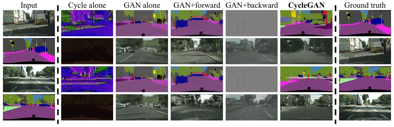
Figure 7: Different variants of our method for mapping labels$\leftrightarrow$photos trained on cityscapes. From left to right: input, cycle-consistency loss alone, adversarial loss alone, GAN + forward cycle-consistency loss ($F(G(x))\approx x$), GAN + backward cycle-consistency loss ($G(F(y))\approx y$), CycleGAN (our full method), and ground truth. Both Cycle alone and GAN + backward fail to produce images similar to the target domain. GAN alone and GAN + forward suffer from mode collapse, producing identical label maps regardless of the input photo.

图 7：我们在城市景观上训练的映射标签$\leftrightarrow$照片的方法的不同变体。 从左到右：输入、单独的循环一致性损失、单独的对抗性损失、GAN + 前向循环一致性损失 ($F(G(x))\approx x$)、GAN + 后向循环一致性损失 ($G(F(y))\approx y$)、CycleGAN （我们的完整方法）和地面事实。 单独循环和GAN +向后都无法生成与目标域相似的图像。 单独的 GAN 和 GAN + 前向 会遭受模式崩溃的影响，无论输入照片如何，都会产生相同的标签图。

Loss	Per-pixel acc.	Per-class acc.	Class IOU
Cycle alone	0.22	0.07	0.02
GAN alone	0.51	0.11	0.08
GAN + forward cycle	0.55	0.18	0.12
GAN + backward cycle	0.39	0.14	0.06
CycleGAN (ours)	0.52	0.17	0.11

Table 4: Ablation study: FCN-scores for different variants of our method, evaluated on Cityscapes labels$\rightarrow$photo.

损失	每像素加速	每班ACC.	类借条
独自骑车	0.22	0.07	0.02
单独生成对抗网络	0.51	0.11	0.08
GAN+前向循环	a68txq8byawaocbjxkf1	5rguec2vzqrooqjekiww	qcd7ef72v7abkn71j65e
GAN+后向循环	0.39	0.14	0.06
CycleGAN（我们的）	0.52	0.17	0.11

表 4：消融研究：我们方法的不同变体的 FCN 分数，在 Cityscapes 标签$\rightarrow$照片上进行评估。

Loss	Per-pixel acc.	Per-class acc.	Class IOU
Cycle alone	0.10	0.05	0.02
GAN alone	0.53	0.11	0.07
GAN + forward cycle	0.49	0.11	0.07
GAN + backward cycle	0.01	0.06	0.01
CycleGAN (ours)	0.58	0.22	0.16

Table 5: Ablation study: classification performance of photo$\rightarrow$labels for different losses, evaluated on Cityscapes.

损失	每像素加速	每班ACC.	类借条
独自骑车	0.10	0.05	0.02
单独生成对抗网络	0.53	0.11	0.07
GAN+前向循环	0.49	0.11	0.07
GAN+后向循环	0.01	0.06	0.01
CycleGAN（我们的）	fq4msuyf5yg6q147txf8	jxrht5ahb9eum48mtuci	ddpoy7rpczehjic9s00a

表 5：消融研究：照片$\rightarrow$标签针对不同损失的分类性能，在 Cityscapes 上进行评估。

5.1.3 Comparison against baselines

As can be seen in Figure 5 and Figure 6, we were unable to achieve compelling results with any of the baselines. Our method, on the other hand, can produce translations that are often of similar quality to the fully supervised pix2pix.

5.1.3 与基线的比较

如图 5 和图 6 所示，我们无法使用任何基线获得令人信服的结果。 另一方面，我们的方法可以生成与完全监督的 pix2pix 质量相似的翻译。

Table 1 reports performance regarding the AMT perceptual realism task. Here, we see that our method can fool participants on around a quarter of trials, in both the maps$\rightarrow$aerial photos direction and the aerial photos$\rightarrow$maps direction at $256\times 256$ resolution[^3]. All the baselines almost never fooled participants.

表 1 报告了 AMT 感知现实主义任务的表现。 在这里，我们看到我们的方法可以在大约四分之一的试验中欺骗参与者，无论是地图$\rightarrow$航空照片方向还是航空照片$\rightarrow$地图方向（分辨率为 $256\times 256$）[^3]。 所有的基线几乎都不会欺骗参与者。

Table 2 assesses the performance of the labels$\rightarrow$photo task on the Cityscapes and Table 3 evaluates the opposite mapping (photos$\rightarrow$labels). In both cases, our method again outperforms the baselines.

表 2 评估了标签$\rightarrow$照片任务在城市景观上的表现，表 3 评估了相反的映射（照片$\rightarrow$标签）。 在这两种情况下，我们的方法再次优于基线。

5.1.4 Analysis of the loss function

In Table 4 and Table 5, we compare against ablations of our full loss. Removing the GAN loss substantially degrades results, as does removing the cycle-consistency loss. We therefore conclude that both terms are critical to our results. We also evaluate our method with the cycle loss in only one direction: GAN + forward cycle loss $\mathbb{E}_{x\sim p_{\text{data}}(x)}[\lVert F(G(x))-x\rVert_{1}]$, or GAN + backward cycle loss $\mathbb{E}_{y\sim p_{\text{data}}(y)}[\lVert G(F(y))-y\rVert_{1}]$ (Equation 2) and find that it often incurs training instability and causes mode collapse, especially for the direction of the mapping that was removed. Figure 7 shows several qualitative examples.

5.1.4 损失函数分析

在表 4 和表 5 中，我们与全部损失的消融进行了比较。 消除 GAN 损失会大大降低结果，消除循环一致性损失也是如此。 因此，我们得出结论，这两个术语对我们的结果都至关重要。 我们还评估了仅在一个方向上的循环损失的方法：GAN + 前向循环损失$\mathbb{E}_{x\sim p_{\text{data}}(x)}[\lVert F(G(x))-x\rVert_{1}]$或 GAN + 后向循环损失 $\mathbb{E}_{y\sim p_{\text{data}}(y)}[\lVert G(F(y))-y\rVert_{1}]$（等式 2），发现它经常会导致训练不稳定并导致模式崩溃，特别是对于被删除的映射方向。 图 7 显示了几个定性示例。

5.1.5 Image reconstruction quality

In Figure 4, we show a few random samples of the reconstructed images $F(G(x))$. We observed that the reconstructed images were often close to the original inputs $x$, at both training and testing time, even in cases where one domain represents significantly more diverse information, such as map$\leftrightarrow$aerial photos.

5.1.5 图像重建质量

在图 4 中，我们显示了重建图像$F(G(x))$的一些随机样本。 我们观察到，在训练和测试时，重建图像通常接近原始输入$x$，即使在一个域代表更加多样化的信息的情况下，例如地图$\leftrightarrow$航空照片也是如此。

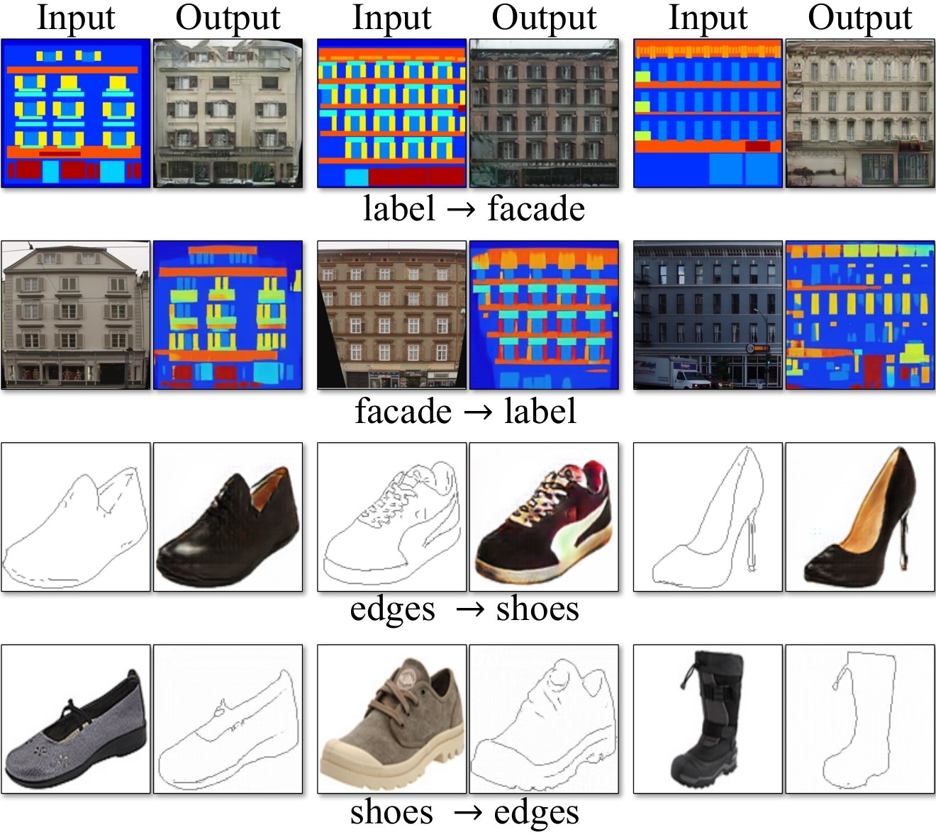
Figure 8: Example results of CycleGAN on paired datasets used in “pix2pix” [22] such as architectural labels$\leftrightarrow$photos and edges$\leftrightarrow$shoes.

图 8：CycleGAN 在“pix2pix”[22] 中使用的配对数据集上的示例结果，例如建筑标签$\leftrightarrow$照片和边缘$\leftrightarrow$鞋子。

5.1.6 Additional results on paired datasets

Figure 8 shows some example results on other paired datasets used in “pix2pix” [22], such as architectural labels$\leftrightarrow$photos from the CMP Facade Database [40], and edges$\leftrightarrow$shoes from the UT Zappos50K dataset [60]. The image quality of our results is close to those produced by the fully supervised pix2pix while our method learns the mapping without paired supervision.

5.1.6 配对数据集的附加结果

图 8 显示了“pix2pix”[22] 中使用的其他配对数据集的一些示例结果，例如来自 CMP Facade Database [40] 的建筑标签$\leftrightarrow$照片，以及来自 UT Zappos50K 数据集 [60] 的边缘$\leftrightarrow$鞋子。 我们的结果的图像质量接近于完全监督的 pix2pix 产生的图像质量，而我们的方法在没有配对监督的情况下学习映射。

5.2 Applications

5.2 应用

We demonstrate our method on several applications where paired training data does not exist. Please refer to the appendix (Section 7) for more details about the datasets. We observe that translations on training data are often more appealing than those on test data, and full results of all applications on both training and test data can be viewed on our project website.

我们在不存在配对训练数据的几个应用程序上演示了我们的方法。 有关数据集的更多详细信息，请参阅附录（第 7 节）。 我们观察到，训练数据的翻译通常比测试数据的翻译更具吸引力，并且可以在我们的项目网站上查看训练和测试数据的所有应用程序的完整结果。

Collection style transfer (Figure 10 and  Figure 11) We train the model on landscape photographs downloaded from Flickr and WikiArt. Unlike recent work on “neural style transfer” [13], our method learns to mimic the style of an entire collection of artworks, rather than transferring the style of a single selected piece of art. Therefore, we can learn to generate photos in the style of, e.g., Van Gogh, rather than just in the style of Starry Night. The size of the dataset for each artist/style was $526$, $1073$, $400$, and $563$ for Cezanne, Monet, Van Gogh, and Ukiyo-e.

收藏风格迁移（图 10 和图 11） 我们使用从 Flickr 和 WikiArt 下载的风景照片来训练模型。 与最近的“神经风格迁移”研究不同[13]，我们的方法学习模仿整个艺术品“收藏”的风格，而不是迁移单个选定艺术品的风格。 因此，我们可以学习生成梵高风格的照片，而不仅仅是星夜风格的照片。 对于塞尚、莫奈、梵高和浮世绘，每个艺术家/风格的数据集大小为$526$、$1073$、$400$和$563$。

Object transfiguration (Figure 13) The model is trained to translate one object class from ImageNet [5] to another (each class contains around $1000$ training images). Turmukhambetov et al. [50] propose a subspace model to translate one object into another object of the same category, while our method focuses on object transfiguration between two visually similar categories.

对象变形（图 13） 该模型经过训练，可将一个对象类别从 ImageNet [5] 转换为另一对象类别（每个类别包含大约$1000$训练图像）。 图尔穆坎贝托夫等人。 [50]提出了一种子空间模型，将一个对象转换为同一类别的另一个对象，而我们的方法侧重于两个视觉相似类别之间的对象变形。

Season transfer (Figure 13) The model is trained on $854$ winter photos and $1273$ summer photos of Yosemite downloaded from Flickr.

季节转移（图 13） 该模型使用从 Flickr 下载的优胜美地$854$冬季照片和$1273$夏季照片进行训练。

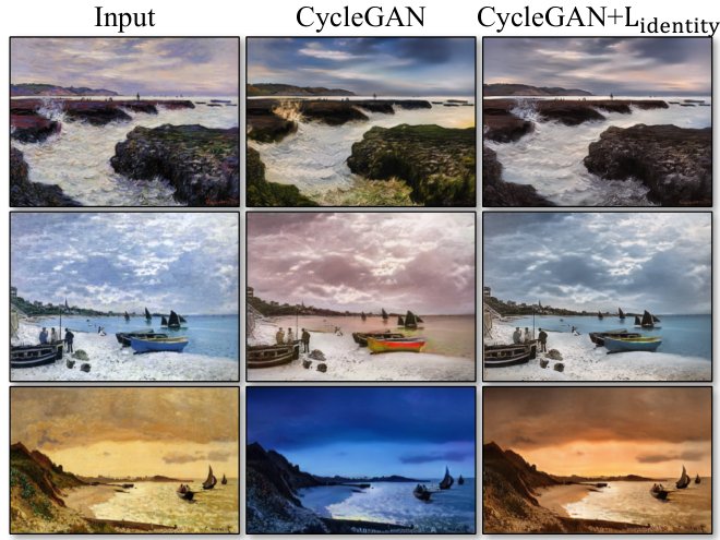
Figure 9: The effect of the identity mapping loss on Monet’s painting$\rightarrow$ photos. From left to right: input paintings, CycleGAN without identity mapping loss, CycleGAN with identity mapping loss. The identity mapping loss helps preserve the color of the input paintings.

图 9：身份映射损失对莫奈绘画$\rightarrow$照片的影响。 从左到右：输入绘画，没有恒等映射损失的 CycleGAN，有恒等映射损失的 CycleGAN。 恒等映射损失有助于保留输入绘画的颜色。

Photo generation from paintings (Figure 12) For painting$\rightarrow$photo, we find that it is helpful to introduce an additional loss to encourage the mapping to preserve color composition between the input and output. In particular, we adopt the technique of Taigman et al. [49] and regularize the generator to be near an identity mapping when real samples of the target domain are provided as the input to the generator: i.e., $\mathcal{L}_{\text{identity}}(G,F)=\mathbb{E}_{y\sim p_{\text{data}}(y)}[\lVert G(y)-y\rVert_{1}]+\mathbb{E}_{x\sim p_{\text{data}}(x)}[\lVert F(x)-x\rVert_{1}].$

从绘画中生成照片（图 12） 对于绘画$\rightarrow$照片，我们发现引入额外的损失有助于鼓励映射保留输入和输出之间的颜色成分。 特别是，我们采用了 Taigman 等人的技术。 [49] 并在提供目标域的真实样本作为生成器的输入时将生成器正则化为接近恒等映射：即 $\mathcal{L}_{\text{identity}}(G,F)=\mathbb{E}_{y\sim p_{\text{data}}(y)}[\lVert G(y)-y\rVert_{1}]+\mathbb{E}_{x\sim p_{\text{data}}(x)}[\lVert F(x)-x\rVert_{1}].$

Without $\mathcal{L}_{\text{identity}}$, the generator $G$ and $F$ are free to change the tint of input images when there is no need to. For example, when learning the mapping between Monet’s paintings and Flickr photographs, the generator often maps paintings of daytime to photographs taken during sunset, because such a mapping may be equally valid under the adversarial loss and cycle consistency loss. The effect of this identity mapping loss are shown in Figure 9.

如果没有$\mathcal{L}_{\text{identity}}$，生成器$G$和$F$可以在不需要时自由更改输入图像的色调。 例如，当学习莫奈的画作和 Flickr 照片之间的映射时，生成器通常将白天的画作映射到日落时拍摄的照片，因为这样的映射在对抗性损失和循环一致性损失下可能同样有效。 这种“身份映射损失”的影响如图 9 所示。

In Figure 12, we show additional results translating Monet’s paintings to photographs. This figure and Figure 9 show results on paintings that were included in the training set, whereas for all other experiments in the paper, we only evaluate and show test set results. Because the training set does not include paired data, coming up with a plausible translation for a training set painting is a nontrivial task. Indeed, since Monet is no longer able to create new paintings, generalization to unseen, “test set”, paintings is not a pressing problem.

在图 12 中，我们展示了将莫奈的画作转化为照片的其他结果。 该图和图 9 显示了“训练集”中包含的绘画结果，而对于本文中的所有其他实验，我们仅评估和显示测试集结果。 由于训练集不包含配对数据，因此为训练集绘制提供合理的翻译是一项艰巨的任务。 事实上，由于莫奈不再能够创作新的绘画，泛化到看不见的“测试集”，绘画并不是一个紧迫的问题。

Photo enhancement (Figure 14) We show that our method can be used to generate photos with shallower depth of field. We train the model on flower photos downloaded from Flickr. The source domain consists of flower photos taken by smartphones, which usually have deep DoF due to a small aperture. The target contains photos captured by DSLRs with a larger aperture. Our model successfully generates photos with shallower depth of field from the photos taken by smartphones.

照片增强（图 14） 我们展示了我们的方法可用于生成景深较浅的照片。 我们使用从 Flickr 下载的花卉照片来训练模型。 源域由智能手机拍摄的花朵照片组成，由于光圈较小，这些照片通常具有深景深。 目标包含具有较大光圈的数码单反相机拍摄的照片。 我们的模型成功地从智能手机拍摄的照片生成景深较浅的照片。

Comparison with Gatys et al. [13] In  Figure 15, we compare our results with neural style transfer [13] on photo stylization. For each row, we first use two representative artworks as the style images for  [13]. Our method, on the other hand, can produce photos in the style of entire collection. To compare against neural style transfer of an entire collection, we compute the average Gram Matrix across the target domain and use this matrix to transfer the “average style” with Gatys et al [13].

与 Gatys 等人的比较。 [13] 在图 15 中，我们将照片风格化的结果与神经风格迁移 [13] 进行比较。 对于每一行，我们首先使用两个代表性艺术品作为[13]的风格图像。 另一方面，我们的方法可以生成整个集合风格的照片。 为了与整个集合的神经风格迁移进行比较，我们计算整个目标域的平均 Gram 矩阵，并使用该矩阵与 Gatys 等人一起迁移“平均风格”[13]。

Figure 16 demonstrates similar comparisons for other translation tasks. We observe that Gatys et al. [13] requires finding target style images that closely match the desired output, but still often fails to produce photorealistic results, while our method succeeds to generate natural-looking results, similar to the target domain.

图 16 展示了其他翻译任务的类似比较。 我们观察到盖蒂斯等人。 [13] 需要找到与所需输出紧密匹配的目标风格图像，但仍然经常无法产生逼真的结果，而我们的方法成功地生成了类似于目标域的自然结果。

6 Limitations and Discussion

6 局限与讨论

Although our method can achieve compelling results in many cases, the results are far from uniformly positive. Figure 17 shows several typical failure cases. On translation tasks that involve color and texture changes, as many of those reported above, the method often succeeds. We have also explored tasks that require geometric changes, with little success. For example, on the task of dog$\rightarrow$cat transfiguration, the learned translation degenerates into making minimal changes to the input (Figure 17). This failure might be caused by our generator architectures which are tailored for good performance on the appearance changes. Handling more varied and extreme transformations, especially geometric changes, is an important problem for future work.

尽管我们的方法在许多情况下可以取得令人信服的结果，但结果远非一致积极。 图 17 显示了几个典型的失败案例。 在涉及颜色和纹理变化的翻译任务中，正如上面报道的许多任务一样，该方法通常会成功。 我们还探索了需要几何变化的任务，但收效甚微。 例如，在狗$\rightarrow$猫变形任务中，学习到的翻译退化为对输入进行最小程度的更改（图 17）。 此故障可能是由我们的生成器架构引起的，该生成器架构是为在外观变化上获得良好性能而定制的。 处理更加多样化和极端的变换，特别是几何变化，是未来工作的一个重要问题。

Some failure cases are caused by the distribution characteristics of the training datasets. For example, our method has got confused in the horse $\rightarrow$ zebra example (Figure 17, right), because our model was trained on the wild horse and zebra synsets of ImageNet, which does not contain images of a person riding a horse or zebra.

一些失败案例是由训练数据集的分布特征引起的。 例如，我们的方法在马$\rightarrow$斑马示例中感到困惑（图 17，右），因为我们的模型是在 ImageNet 的 野马 和 斑马 同义词集上训练的，其中不包含骑着马或斑马的人的图像。

We also observe a lingering gap between the results achievable with paired training data and those achieved by our unpaired method. In some cases, this gap may be very hard – or even impossible – to close: for example, our method sometimes permutes the labels for tree and building in the output of the photos$\rightarrow$labels task. Resolving this ambiguity may require some form of weak semantic supervision. Integrating weak or semi-supervised data may lead to substantially more powerful translators, still at a fraction of the annotation cost of the fully-supervised systems.

我们还观察到使用配对训练数据可实现的结果与通过我们的未配对方法实现的结果之间存在挥之不去的差距。 在某些情况下，这种差距可能非常难以（甚至不可能）弥补：例如，我们的方法有时会在照片$\rightarrow$标签任务的输出中排列树和构建的标签。 解决这种歧义可能需要某种形式的弱语义监督。 集成弱或半监督数据可能会产生更强大的翻译器，而注释成本仍然只是完全监督系统的一小部分。

Nonetheless, in many cases completely unpaired data is plentifully available and should be made use of. This paper pushes the boundaries of what is possible in this “unsupervised” setting.

尽管如此，在许多情况下，完全不配对的数据是大量可用的，应该加以利用。 本文突破了这种“无监督”环境中可能发生的事情的界限。

Acknowledgments: We thank Aaron Hertzmann, Shiry Ginosar, Deepak Pathak, Bryan Russell, Eli Shechtman, Richard Zhang, and Tinghui Zhou for many helpful comments. This work was supported in part by NSF SMA-1514512, NSF IIS-1633310, a Google Research Award, Intel Corp, and hardware donations from NVIDIA. JYZ is supported by the Facebook Graduate Fellowship and TP is supported by the Samsung Scholarship. The photographs used for style transfer were taken by AE, mostly in France.

致谢： 我们感谢 Aaron Hertzmann、Shiry Ginosar、Deepak Pathak、Bryan Russell、Eli Shechtman、Richard 张和 Tinghui Zhou 提供的许多有用的评论。 这项工作得到了 NSF SMA-1514512、NSF IIS-1633310、Google 研究奖、英特尔公司以及 NVIDIA 硬件捐赠的部分支持。 JYZ 得到 Facebook 研究生奖学金的支持，TP 得到三星奖学金的支持。 用于风格转移的照片由AE拍摄，大部分在法国。

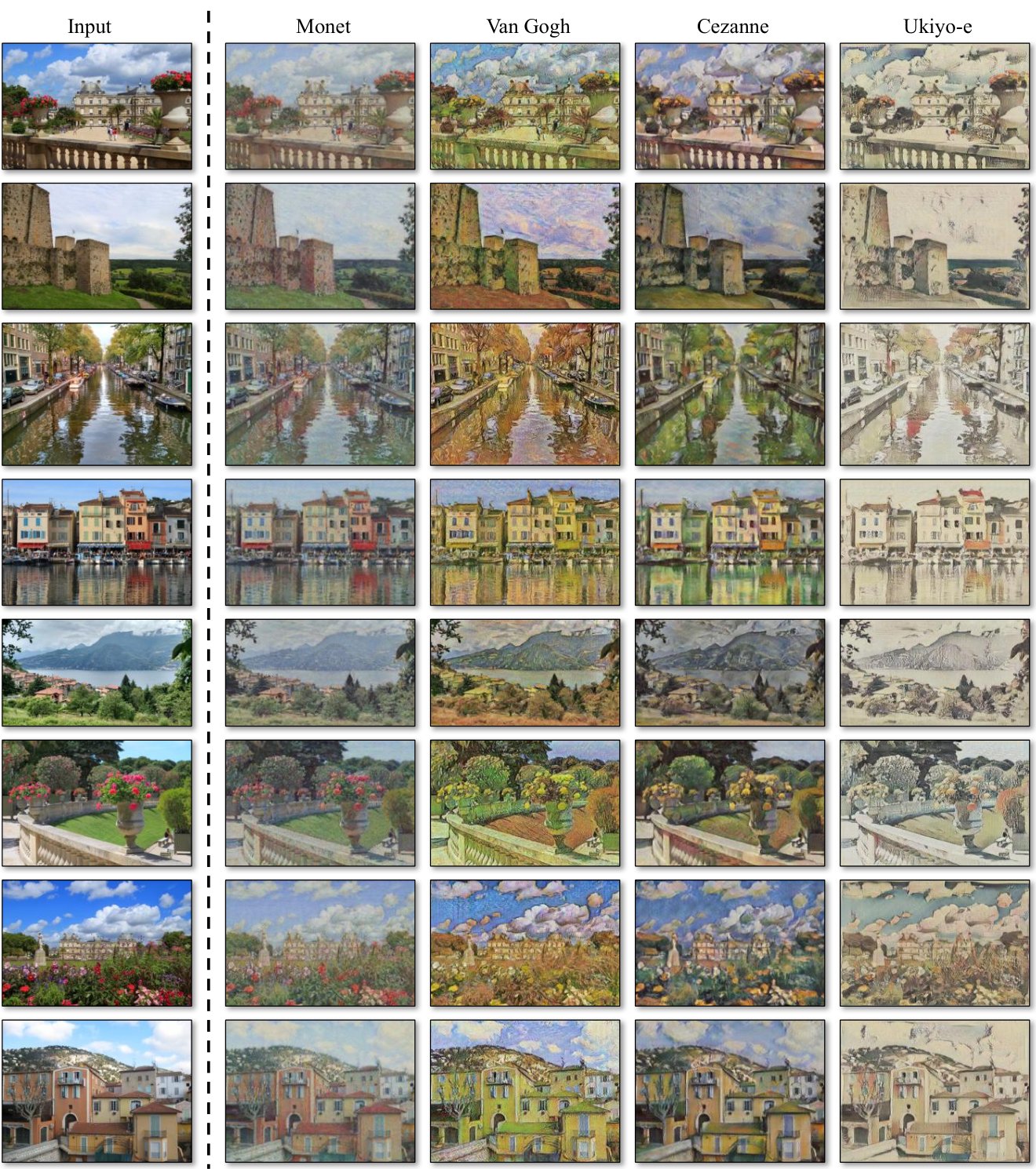
Figure 10: Collection style transfer I: we transfer input images into the artistic styles of Monet, Van Gogh, Cezanne, and Ukiyo-e. Please see our website for additional examples.

图 10：收藏风格转换 I：我们将输入图像转换为莫奈、梵高、塞尚和浮世绘的艺术风格。 请参阅我们的网站了解更多示例。

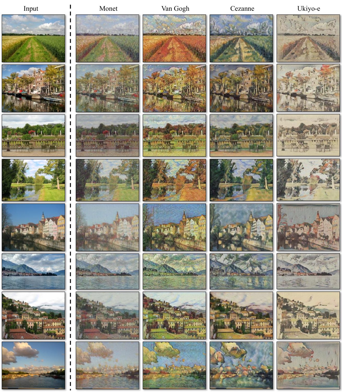
Figure 11: Collection style transfer II: we transfer input images into the artistic styles of Monet, Van Gogh, Cezanne, Ukiyo-e. Please see our website for additional examples.

图11：收藏风格转换II：我们将输入图像转换为莫奈、梵高、塞尚、浮世绘的艺术风格。 请参阅我们的网站了解更多示例。

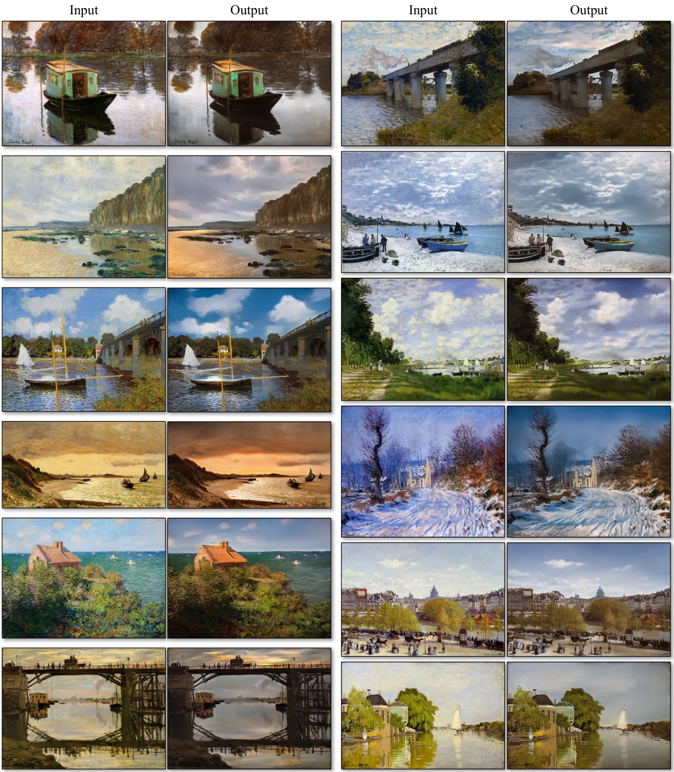
Figure 12: Relatively successful results on mapping Monet’s paintings to a photographic style. Please see our website for additional examples.

图 12：将莫奈的画作映射到摄影风格方面取得了相对成功的结果。 请参阅我们的网站了解更多示例。

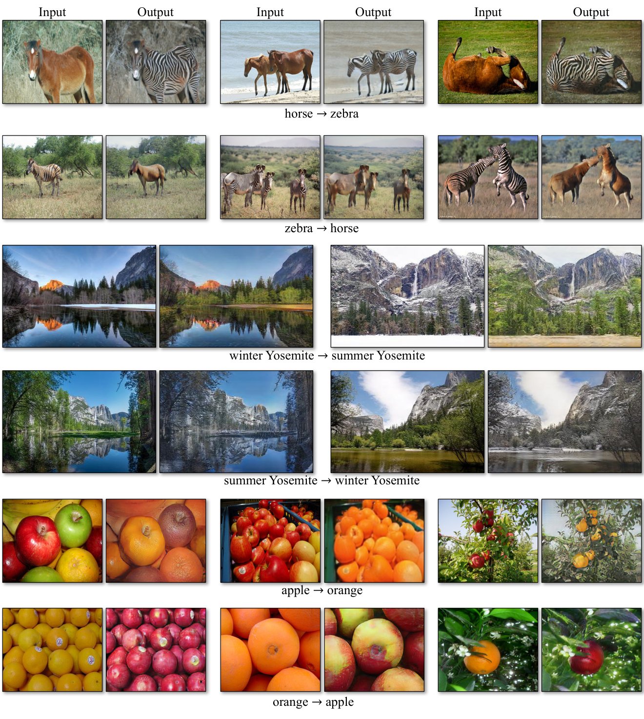
Figure 13: Our method applied to several translation problems. These images are selected as relatively successful results – please see our website for more comprehensive and random results. In the top two rows, we show results on object transfiguration between horses and zebras, trained on 939 images from the wild horse class and 1177 images from the zebra class in Imagenet [5]. Also check out the horse$\rightarrow$zebra demo video. The middle two rows show results on season transfer, trained on winter and summer photos of Yosemite from Flickr. In the bottom two rows, we train our method on 996 apple images and 1020 navel orange images from ImageNet.

图 13：我们的方法应用于多个翻译问题。 这些图像被选为相对成功的结果 - 请访问我们的网站以获取更全面和随机的结果。 在顶部两行中，我们显示了马和斑马之间的对象变形结果，这些结果是在 Imagenet [5] 中的 野马 类的 939 张图像和 斑马 类的 1177 张图像上进行训练的。 另请观看马$\rightarrow$斑马演示视频。 中间两行显示季节转移的结果，根据 Flickr 上优胜美地的冬季和夏季照片进行训练。 在底部两行中，我们在 ImageNet 中的 996 张苹果图像和 1020 张脐橙图像上训练我们的方法。

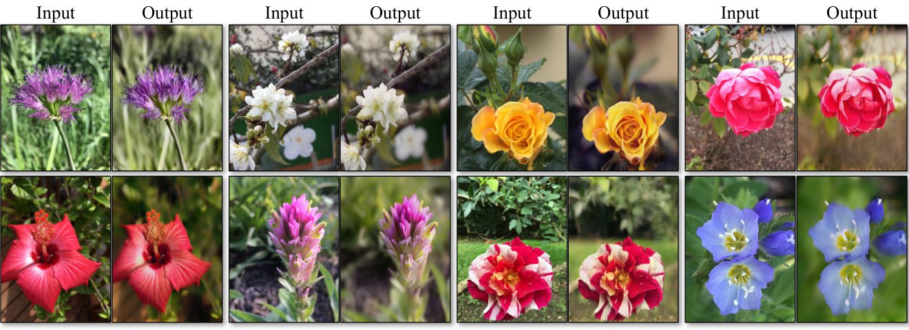
Figure 14: Photo enhancement: mapping from a set of smartphone snaps to professional DSLR photographs, the system often learns to produce shallow focus. Here we show some of the most successful results in our test set – average performance is considerably worse. Please see our website for more comprehensive and random examples.

图 14：照片增强：从一组智能手机快照映射到专业 DSLR 照片，系统通常会学习产生浅焦点。 在这里，我们展示了测试集中一些最成功的结果——平均性能要差得多。 请访问我们的网站以获取更全面和随机的示例。

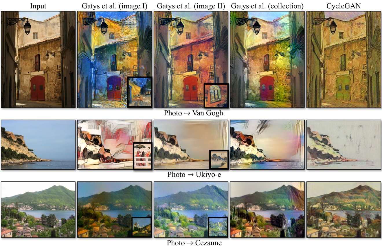
Figure 15: We compare our method with neural style transfer [13] on photo stylization. Left to right: input image, results from Gatys et al. [13] using two different representative artworks as style images, results from Gatys et al. [13] using the entire collection of the artist, and CycleGAN (ours).

图 15：我们将我们的方法与照片风格化方面的神经风格迁移 [13] 进行比较。 从左到右：输入图像，Gatys 等人的结果。 [13]使用两种不同的代表性艺术品作为风格图像，来自 Gatys 等人的结果。 [13] 使用艺术家和 CycleGAN（我们的）的整个收藏。

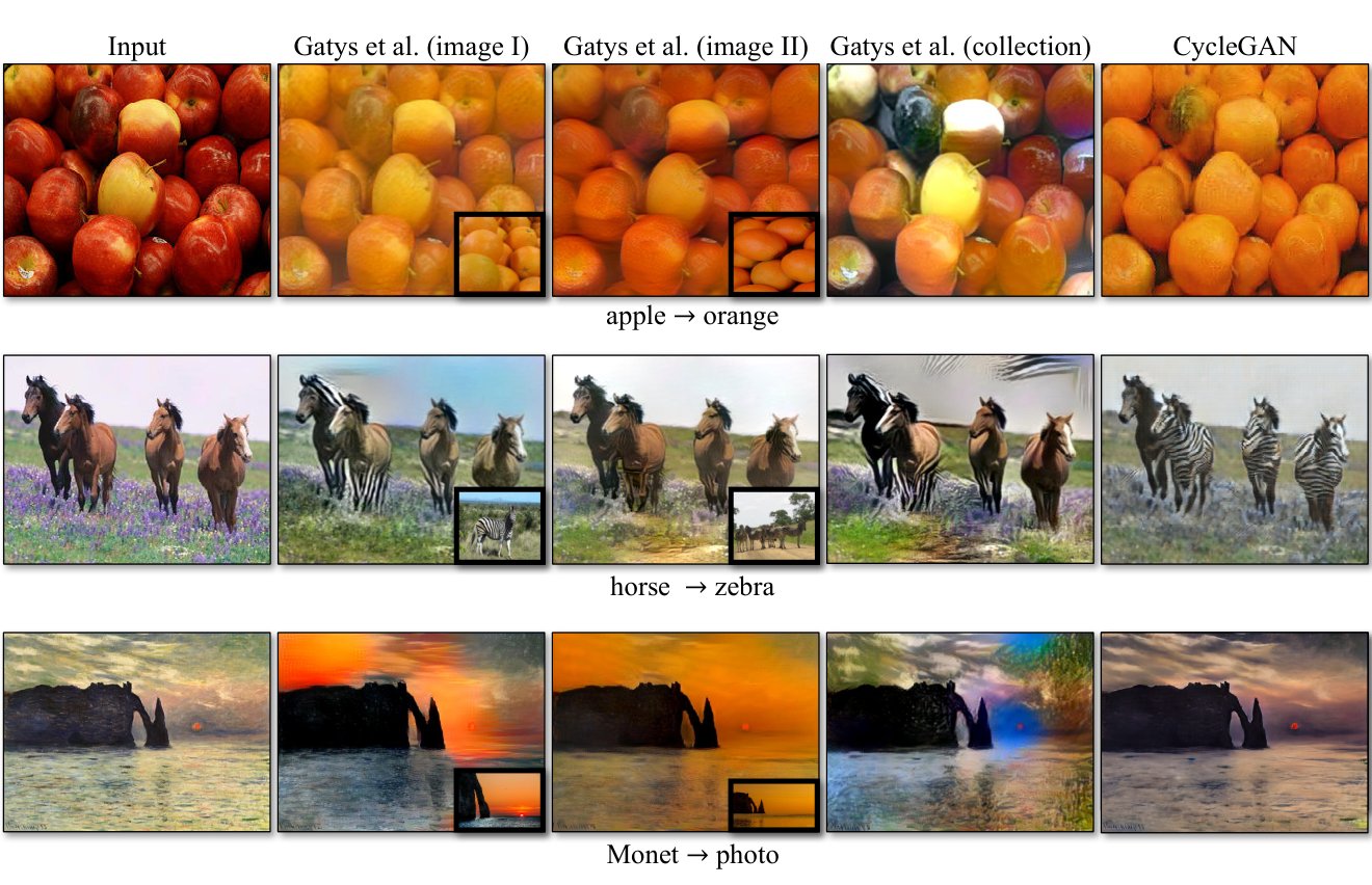
Figure 16: We compare our method with neural style transfer [13] on various applications. From top to bottom: apple$\rightarrow$orange, horse$\rightarrow$zebra, and Monet$\rightarrow$photo. Left to right: input image, results from Gatys et al. [13] using two different images as style images, results from Gatys et al. [13] using all the images from the target domain, and CycleGAN (ours).

图 16：我们在各种应用中将我们的方法与神经风格迁移 [13] 进行比较。 从上到下：苹果$\rightarrow$橙色，马$\rightarrow$斑马，莫奈$\rightarrow$照片。 从左到右：输入图像，Gatys 等人的结果。 [13] 使用两个不同的图像作为风格图像，来自 Gatys 等人的结果。 [13] 使用目标域中的所有图像和 CycleGAN（我们的）。

(a)

（一个）

References

参考文献

[1] Y. Aytar, L. Castrejon, C. Vondrick, H. Pirsiavash, and A. Torralba. Cross-modal scene networks. PAMI , 2016.

[2] K. Bousmalis, N. Silberman, D. Dohan, D. Erhan, and D. Krishnan. Unsupervised pixel-level domain adaptation with generative adversarial networks. In CVPR , 2017.

[3] R. W. Brislin. Back-translation for cross-cultural research. Journal of cross-cultural psychology , 1(3):185–216, 1970.

[4] M. Cordts, M. Omran, S. Ramos, T. Rehfeld, M. Enzweiler, R. Benenson, U. Franke, S. Roth, and B. Schiele. The cityscapes dataset for semantic urban scene understanding. In CVPR , 2016.

[5] J. Deng, W. Dong, R. Socher, L.-J. Li, K. Li, and L. Fei-Fei. Imagenet: A large-scale hierarchical image database. In CVPR , 2009.

[6] E. L. Denton, S. Chintala, R. Fergus, et al. Deep generative image models using a laplacian pyramid of adversarial networks. In NIPS , 2015.

[7] J. Donahue, P. Krähenbühl, and T. Darrell. Adversarial feature learning. In ICLR , 2017.

[8] A. Dosovitskiy and T. Brox. Generating images with perceptual similarity metrics based on deep networks. In NIPS , 2016.

[9] V. Dumoulin, I. Belghazi, B. Poole, A. Lamb, M. Arjovsky, O. Mastropietro, and A. Courville. Adversarially learned inference. In ICLR , 2017.

[10] A. A. Efros and T. K. Leung. Texture synthesis by non-parametric sampling. In ICCV , 1999.

[11] D. Eigen and R. Fergus. Predicting depth, surface normals and semantic labels with a common multi-scale convolutional architecture. In ICCV , 2015.

[12] L. A. Gatys, M. Bethge, A. Hertzmann, and E. Shechtman. Preserving color in neural artistic style transfer. arXiv preprint arXiv:1606.05897 , 2016.

[13] L. A. Gatys, A. S. Ecker, and M. Bethge. Image style transfer using convolutional neural networks. CVPR , 2016.

[14] C. Godard, O. Mac Aodha, and G. J. Brostow. Unsupervised monocular depth estimation with left-right consistency. In CVPR , 2017.

[15] I. Goodfellow. NIPS 2016 tutorial: Generative adversarial networks. arXiv preprint arXiv:1701.00160 , 2016.

[16] I. Goodfellow, J. Pouget-Abadie, M. Mirza, B. Xu, D. Warde-Farley, S. Ozair, A. Courville, and Y. Bengio. Generative adversarial nets. In NIPS , 2014.

[17] D. He, Y. Xia, T. Qin, L. Wang, N. Yu, T. Liu, and W.-Y. Ma. Dual learning for machine translation. In NIPS , 2016.

[18] K. He, X. Zhang, S. Ren, and J. Sun. Deep residual learning for image recognition. In CVPR , 2016.

[19] A. Hertzmann, C. E. Jacobs, N. Oliver, B. Curless, and D. H. Salesin. Image analogies. In SIGGRAPH , 2001.

[20] G. E. Hinton and R. R. Salakhutdinov. Reducing the dimensionality of data with neural networks. Science , 313(5786):504–507, 2006.

[21] Q.-X. Huang and L. Guibas. Consistent shape maps via semidefinite programming. In Symposium on Geometry Processing , 2013.

[22] P. Isola, J.-Y. Zhu, T. Zhou, and A. A. Efros. Image-to-image translation with conditional adversarial networks. In CVPR , 2017.

[23] J. Johnson, A. Alahi, and L. Fei-Fei. Perceptual losses for real-time style transfer and super-resolution. In ECCV , 2016.

[24] Z. Kalal, K. Mikolajczyk, and J. Matas. Forward-backward error: Automatic detection of tracking failures. In ICPR , 2010.

[25] L. Karacan, Z. Akata, A. Erdem, and E. Erdem. Learning to generate images of outdoor scenes from attributes and semantic layouts. arXiv preprint arXiv:1612.00215 , 2016.

[26] D. Kingma and J. Ba. Adam: A method for stochastic optimization. In ICLR , 2015.

[27] D. P. Kingma and M. Welling. Auto-encoding variational bayes. ICLR , 2014.

[28] P.-Y. Laffont, Z. Ren, X. Tao, C. Qian, and J. Hays. Transient attributes for high-level understanding and editing of outdoor scenes. ACM TOG , 33(4):149, 2014.

[29] C. Ledig, L. Theis, F. Huszár, J. Caballero, A. Cunningham, A. Acosta, A. Aitken, A. Tejani, J. Totz, Z. Wang, et al. Photo-realistic single image super-resolution using a generative adversarial network. In CVPR , 2017.

[30] C. Li and M. Wand. Precomputed real-time texture synthesis with markovian generative adversarial networks. ECCV , 2016.

[31] M.-Y. Liu, T. Breuel, and J. Kautz. Unsupervised image-to-image translation networks. In NIPS , 2017.

[32] M.-Y. Liu and O. Tuzel. Coupled generative adversarial networks. In NIPS , 2016.

[33] J. Long, E. Shelhamer, and T. Darrell. Fully convolutional networks for semantic segmentation. In CVPR , 2015.

[34] A. Makhzani, J. Shlens, N. Jaitly, I. Goodfellow, and B. Frey. Adversarial autoencoders. In ICLR , 2016.

[35] X. Mao, Q. Li, H. Xie, R. Y. Lau, Z. Wang, and S. P. Smolley. Least squares generative adversarial networks. In CVPR . IEEE, 2017.

[36] M. Mathieu, C. Couprie, and Y. LeCun. Deep multi-scale video prediction beyond mean square error. In ICLR , 2016.

[37] M. F. Mathieu, J. Zhao, A. Ramesh, P. Sprechmann, and Y. LeCun. Disentangling factors of variation in deep representation using adversarial training. In NIPS , 2016.

[38] D. Pathak, P. Krahenbuhl, J. Donahue, T. Darrell, and A. A. Efros. Context encoders: Feature learning by inpainting. CVPR , 2016.

[39] A. Radford, L. Metz, and S. Chintala. Unsupervised representation learning with deep convolutional generative adversarial networks. In ICLR , 2016.

[40] R. Š. Radim Tyleček. Spatial pattern templates for recognition of objects with regular structure. In Proc. GCPR , Saarbrucken, Germany, 2013.

[41] S. Reed, Z. Akata, X. Yan, L. Logeswaran, B. Schiele, and H. Lee. Generative adversarial text to image synthesis. In ICML , 2016.

[42] R. Rosales, K. Achan, and B. J. Frey. Unsupervised image translation. In ICCV , 2003.

[43] T. Salimans, I. Goodfellow, W. Zaremba, V. Cheung, A. Radford, and X. Chen. Improved techniques for training GANs. In NIPS , 2016.

[44] P. Sangkloy, J. Lu, C. Fang, F. Yu, and J. Hays. Scribbler: Controlling deep image synthesis with sketch and color. In CVPR , 2017.

[45] Y. Shih, S. Paris, F. Durand, and W. T. Freeman. Data-driven hallucination of different times of day from a single outdoor photo. ACM TOG , 32(6):200, 2013.

[46] A. Shrivastava, T. Pfister, O. Tuzel, J. Susskind, W. Wang, and R. Webb. Learning from simulated and unsupervised images through adversarial training. In CVPR , 2017.

[47] K. Simonyan and A. Zisserman. Very deep convolutional networks for large-scale image recognition. In ICLR , 2015.

[48] N. Sundaram, T. Brox, and K. Keutzer. Dense point trajectories by gpu-accelerated large displacement optical flow. In ECCV , 2010.

[49] Y. Taigman, A. Polyak, and L. Wolf. Unsupervised cross-domain image generation. In ICLR , 2017.

[50] D. Turmukhambetov, N. D. Campbell, S. J. Prince, and J. Kautz. Modeling object appearance using context-conditioned component analysis. In CVPR , 2015.

[51] M. Twain. The jumping frog: in english, then in french, and then clawed back into a civilized language once more by patient. Unremunerated Toil , 3, 1903.

[52] D. Ulyanov, V. Lebedev, A. Vedaldi, and V. Lempitsky. Texture networks: Feed-forward synthesis of textures and stylized images. In ICML , 2016.

[53] D. Ulyanov, A. Vedaldi, and V. Lempitsky. Instance normalization: The missing ingredient for fast stylization. arXiv preprint arXiv:1607.08022 , 2016.

[54] C. Vondrick, H. Pirsiavash, and A. Torralba. Generating videos with scene dynamics. In NIPS , 2016.

[55] F. Wang, Q. Huang, and L. J. Guibas. Image co-segmentation via consistent functional maps. In ICCV , 2013.

[56] X. Wang and A. Gupta. Generative image modeling using style and structure adversarial networks. In ECCV , 2016.

[57] J. Wu, C. Zhang, T. Xue, B. Freeman, and J. Tenenbaum. Learning a probabilistic latent space of object shapes via 3d generative-adversarial modeling. In NIPS , 2016.

[58] S. Xie and Z. Tu. Holistically-nested edge detection. In ICCV , 2015.

[59] Z. Yi, H. Zhang, T. Gong, Tan, and M. Gong. Dualgan: Unsupervised dual learning for image-to-image translation. In ICCV , 2017.

[60] A. Yu and K. Grauman. Fine-grained visual comparisons with local learning. In CVPR , 2014.

[61] C. Zach, M. Klopschitz, and M. Pollefeys. Disambiguating visual relations using loop constraints. In CVPR , 2010.

[62] R. Zhang, P. Isola, and A. A. Efros. Colorful image colorization. In ECCV , 2016.

[63] J. Zhao, M. Mathieu, and Y. LeCun. Energy-based generative adversarial network. In ICLR , 2017.

[64] T. Zhou, P. Krahenbuhl, M. Aubry, Q. Huang, and A. A. Efros. Learning dense correspondence via 3d-guided cycle consistency. In CVPR , 2016.

[65] T. Zhou, Y. J. Lee, S. Yu, and A. A. Efros. Flowweb: Joint image set alignment by weaving consistent, pixel-wise correspondences. In CVPR , 2015.

[66] J.-Y. Zhu, P. Krähenbühl, E. Shechtman, and A. A. Efros. Generative visual manipulation on the natural image manifold. In ECCV , 2016.

7 Appendix

7 附录

7.1 Training details

7.1 训练细节

We train our networks from scratch, with a learning rate of $0.0002$. In practice, we divide the objective by $2$ while optimizing $D$, which slows down the rate at which $D$ learns, relative to the rate of $G$. We keep the same learning rate for the first $100$ epochs and linearly decay the rate to zero over the next $100$ epochs. Weights are initialized from a Gaussian distribution $\mathcal{N}(0,0.02)$.

我们从头开始训练我们的网络，学习率为$0.0002$。 在实践中，我们在优化$D$的同时将目标除以$2$，相对于$G$的速度，这会减慢$D$的学习速度。 我们在前$100$时期保持相同的学习率，并在接下来的$100$时期将学习率线性衰减到零。 权重从高斯分布$\mathcal{N}(0,0.02)$初始化。

Cityscapes label$\leftrightarrow$Photo $2975$ training images from the Cityscapes training set [4] with image size $128\times 128$. We used the Cityscapes val set for testing.

Cityscapes 标签$\leftrightarrow$照片$2975$训练图像来自 Cityscapes 训练集 [4]，图像大小为$128\times 128$。 我们使用 Cityscapes val 集进行测试。

Maps$\leftrightarrow$aerial photograph $1096$ training images were scraped from Google Maps [22] with image size $256\times 256$. Images were sampled from in and around New York City. Data was then split into train and test about the median latitude of the sampling region (with a buffer region added to ensure that no training pixel appeared in the test set).

地图$\leftrightarrow$航拍照片$1096$训练图像是从 Google 地图 [22] 中抓取的，图像大小为$256\times 256$。 图像取自纽约市及其周边地区。 然后将数据分成关于采样区域的中值纬度的训练和测试（添加缓冲区以确保测试集中没有训练像素出现）。

Architectural facades labels$\leftrightarrow$photo $400$ training images from the CMP Facade Database [40].

建筑立面标签$\leftrightarrow$照片$400$训练图像来自 CMP Facade 数据库 [40]。

Edges$\rightarrow$shoes around $50,000$ training images from UT Zappos50K dataset [60]. The model was trained for $5$ epochs.

边缘$\rightarrow$鞋围绕来自 UT Zappos50K 数据集的$50,000$训练图像[60]。 该模型接受了$5$轮次的训练。

Horse$\leftrightarrow$Zebra and Apple$\leftrightarrow$Orange We downloaded the images from ImageNet [5] using keywords wild horse, zebra, apple, and navel orange. The images were scaled to $256\times 256$ pixels. The training set size of each class: $939$ (horse), $1177$ (zebra), $996$ (apple), and $1020$ (orange).

马$\leftrightarrow$斑马和苹果$\leftrightarrow$橙色 我们使用关键字 野马、斑马、苹果和脐橙从 ImageNet [5] 下载图像。 图像缩放至$256\times 256$像素。 每个类别的训练集大小：$939$（马）、$1177$（斑马）、$996$（苹果）和$1020$（橙色）。

Summer$\leftrightarrow$Winter Yosemite The images were downloaded using Flickr API with the tag yosemite and the datetaken field. Black-and-white photos were pruned. The images were scaled to $256\times 256$ pixels. The training size of each class: $1273$ (summer) and $854$ ( winter).

夏季$\leftrightarrow$冬季 Yosemite 这些图像是使用 Flickr API 以及标签 yosemite 和 datetaken 字段下载的。 黑白照片被修剪。 图像缩放至$256\times 256$像素。 每班训练规模：$1273$（夏季）和$854$（冬季）。

Photo$\leftrightarrow$Art for style transfer The art images were downloaded from Wikiart.org. Some artworks that were sketches or too obscene were pruned by hand. The photos were downloaded from Flickr using the combination of tags landscape and landscapephotography. Black-and-white photos were pruned. The images were scaled to $256\times 256$ pixels. The training set size of each class was $1074$ (Monet), $584$ (Cezanne), $401$ (Van Gogh), $1433$ (Ukiyo-e), and $6853$ (Photographs). The Monet dataset was particularly pruned to include only landscape paintings, and the Van Gogh dataset included only his later works that represent his most recognizable artistic style.

照片$\leftrightarrow$风格转移艺术 艺术图像是从 Wikiart.org 下载的。 一些草图或过于淫秽的艺术品被手工修剪。 这些照片是使用标签 landscape 和 landscapephotography 的组合从 Flickr 下载的。 黑白照片被修剪。 图像缩放至$256\times 256$像素。 每个类别的训练集大小为$1074$（莫奈）、$584$（塞尚）、$401$（梵高）、$1433$（浮世绘）和$6853$（照片）。 莫奈数据集经过特别修剪，仅包含风景画，梵高数据集仅包含他后期代表其最知名艺术风格的作品。

Monet’s paintings$\rightarrow$photos To achieve high resolution while conserving memory, we used random square crops of the original images for training. To generate results, we passed images of width $512$ pixels with correct aspect ratio to the generator network as input. The weight for the identity mapping loss was $0.5\lambda$ where $\lambda$ was the weight for cycle consistency loss. We set $\lambda=10$.

莫奈的画作$\rightarrow$照片 为了在节省内存的同时实现高分辨率，我们使用原始图像的随机方形裁剪进行训练。 为了生成结果，我们将具有正确宽高比的宽度$512$像素的图像传递给生成器网络作为输入。 身份映射损失的权重是 $0.5\lambda$，其中$\lambda$是循环一致性损失的权重。 我们设置$\lambda=10$。

Flower photo enhancement Flower images taken on smartphones were downloaded from Flickr by searching for the photos taken by Apple iPhone 5, 5s, or 6, with search text flower. DSLR images with shallow DoF were also downloaded from Flickr by search tag flower, dof. The images were scaled to $360$ pixels by width. The identity mapping loss of weight $0.5\lambda$ was used. The training set size of the smartphone and DSLR dataset were $1813$ and $3326$, respectively. We set $\lambda=10$.

花卉照片增强 在智能手机上拍摄的花卉图像是通过搜索 Apple iPhone 5、5s 或 6 拍摄的照片从 Flickr 下载的，搜索文本为 flower。 还可以通过搜索标签 flower, dof 从 Flickr 下载具有浅景深的 DSLR 图像。 图像按宽度缩放至$360$像素。 使用恒等映射权重损失 $0.5\lambda$。 智能手机和 DSLR 数据集的训练集大小分别为$1813$和$3326$。 我们设置$\lambda=10$。

7.2 Network architectures

7.2 网络架构

We provide both PyTorch and Torch implementations.

我们提供 PyTorch 和 Torch 实现。

Generator architectures We adopt our architectures from Johnson et al. [23]. We use $6$ residual blocks for $128\times 128$ training images, and $9$ residual blocks for $256\times 256$ or higher-resolution training images. Below, we follow the naming convention used in the Johnson et al.’s Github repository.

生成器架构 我们采用 Johnson 等人的架构。 [23]。 我们对$128\times 128$训练图像使用$6$残差块，对$256\times 256$或更高分辨率的训练图像使用$9$残差块。 下面，我们遵循 Johnson 等人的 Github 存储库中使用的命名约定。

Let c7s1-k denote a $7\times 7$ Convolution-InstanceNorm-ReLU layer with $k$ filters and stride $1$. dk denotes a $3\times 3$ Convolution-InstanceNorm-ReLU layer with $k$ filters and stride $2$. Reflection padding was used to reduce artifacts. Rk denotes a residual block that contains two $3\times 3$ convolutional layers with the same number of filters on both layer. uk denotes a $3\times 3$ fractional-strided-Convolution-InstanceNorm-ReLU layer with $k$ filters and stride $\frac{1}{2}$.

令 c7s1-k 表示具有$k$滤波器和跨度$1$的$7\times 7$Convolution-InstanceNorm-ReLU 层。 dk 表示具有$k$滤波器和步幅$2$的$3\times 3$Convolution-InstanceNorm-ReLU 层。 使用反射填充来减少伪影。 Rk 表示包含两个$3\times 3$卷积层的残差块，两层上的滤波器数量相同。 uk 表示具有$k$滤波器和步幅$\frac{1}{2}$的$3\times 3$分数跨步卷积-InstanceNorm-ReLU 层。

The network with 6 residual blocks consists of: c7s1-64,d128,d256,R256,R256,R256, R256,R256,R256,u128,u64,c7s1-3

具有 6 个残差块的网络包括：c7s1-64,d128,d256,R256,R256,R256, R256,R256,R256,u128,u64,c7s1-3

The network with 9 residual blocks consists of: c7s1-64,d128,d256,R256,R256,R256, R256,R256,R256,R256,R256,R256,u128 u64,c7s1-3

具有 9 个残差块的网络包括：c7s1-64,d128,d256,R256,R256,R256, R256,R256,R256,R256,R256,R256,u128 u64,c7s1-3

Discriminator architectures For discriminator networks, we use $70\times 70$ PatchGAN [22]. Let Ck denote a $4\times 4$ Convolution-InstanceNorm-LeakyReLU layer with k filters and stride $2$. After the last layer, we apply a convolution to produce a $1$-dimensional output. We do not use InstanceNorm for the first C64 layer. We use leaky ReLUs with a slope of $0.2$. The discriminator architecture is: C64-C128-C256-C512

鉴别器架构 对于鉴别器网络，我们使用$70\times 70$PatchGAN [22]。 令 Ck 表示具有 k 个滤波器且步幅为$2$的$4\times 4$Convolution-InstanceNorm-LeakyReLU 层。 在最后一层之后，我们应用卷积来产生$1$维输出。 我们不对第一个 C64 层使用 InstanceNorm。 我们使用斜率为$0.2$的leaky ReLU。 鉴别器架构为：C64-C128-C256-C512