CutMix: Regularization Strategy to Train Strong Classifiers with Localizable Features

CutMix：用可定位特征训练强分类器的正则化策略

Sangdoo Yun         Dongyoon Han         Seong Joon Oh         Sanghyuk Chun Affiliation:  Clova AI Research, NAVER Corp. Affiliation:  Clova AI Research, NAVER Corp. Affiliation:  Clova AI Research, NAVER Corp. Affiliation:  Clova AI Research, LINE Plus Corp.    Junsuk Choe        Youngjoon Yoo Affiliation:  Clova AI Research, NAVER Corp. Affiliation:  Clova AI Research, NAVER Corp. Affiliation:  Yonsei University

Abstract

摘要

Regional dropout strategies have been proposed to enhance the performance of convolutional neural network classifiers. They have proved to be effective for guiding the model to attend on less discriminative parts of objects (e.g. leg as opposed to head of a person), thereby letting the network generalize better and have better object localization capabilities. On the other hand, current methods for regional dropout remove informative pixels on training images by overlaying a patch of either black pixels or random noise. Such removal is not desirable because it leads to information loss and inefficiency during training. We therefore propose the CutMix augmentation strategy: patches are cut and pasted among training images where the ground truth labels are also mixed proportionally to the area of the patches. By making efficient use of training pixels and retaining the regularization effect of regional dropout, CutMix consistently outperforms the state-of-the-art augmentation strategies on CIFAR and ImageNet classification tasks, as well as on the ImageNet weakly-supervised localization task. Moreover, unlike previous augmentation methods, our CutMix-trained ImageNet classifier, when used as a pretrained model, results in consistent performance gains in Pascal detection and MS-COCO image captioning benchmarks. We also show that CutMix improves the model robustness against input corruptions and its out-of-distribution detection performances. Source code and pretrained models are available at https://github.com/clovaai/CutMix-PyTorch.

区域 dropout 策略被提出用于提升卷积神经网络分类器性能。它们能有效引导模型关注物体上区分度较低的部位（例如人的腿而不是头），从而让网络泛化更好，并具备更好的目标定位能力。另一方面，现有区域 dropout 方法通过叠加一块黑像素或随机噪声补丁，从训练图像上去除信息性像素。这种去除并不理想，因为它会造成信息损失与训练低效。因此我们提出 CutMix 增强策略：在训练图像之间剪切并粘贴补丁，同时按补丁面积比例混合真实标签。通过高效利用训练像素并保留区域 dropout 的正则化效果，CutMix 在 CIFAR 与 ImageNet 分类任务以及 ImageNet 弱监督定位任务上持续优于当时最优增强策略。此外，与先前增强方法不同，经 CutMix 训练的 ImageNet 分类器作为预训练模型时，在 Pascal 检测与 MS-COCO 图像描述上带来稳定增益。最后，我们分析并证明：CutMix 改善模型对输入损坏与样本超出训练集分布时的鲁棒性与不确定性。

1 Introduction

1 引言

Deep convolutional neural networks (CNNs) have shown promising performances on various computer vision problems such as image classification [31, 20, 12], object detection [30, 24], semantic segmentation [1, 25], and video analysis [28, 32]. To further improve the training efficiency and performance, a number of training strategies have been proposed, including data augmentation [20] and regularization techniques [34, 17, 38].

深度卷积神经网络（CNN）在各类计算机视觉识别任务上表现出色。然而，它们往往过度依赖一小部分判别性输入区域或中间激活，导致泛化变差，也削弱了定位物体完整范围的能力。

In particular, to prevent a CNN from focusing too much on a small set of intermediate activations or on a small region on input images, random feature removal regularizations have been proposed. Examples include dropout [34] for randomly dropping hidden activations and regional dropout [3, 51, 33, 8, 2] for erasing random regions on the input. Researchers have shown that the feature removal strategies improve generalization and localization by letting a model attend not only to the most discriminative parts of objects, but rather to the entire object region [33, 8].

尤其是，为防止 CNN 过度聚焦于一小部分中间激活或局部判别部位，已有工作提出在特征图或输入图像上做区域 dropout。这类方法被证明能提升分类精度，并改善弱监督目标定位，因为模型学会关注物体更广泛的部位。

	ResNet-50	Mixup [48]	Cutout [3]	CutMix
Image
Label	Dog 1.0	Dog 0.5 Cat 0.5	Dog 1.0	Dog 0.6 Cat 0.4
ImageNet Cls (%)	76.3 (+0.0)	77.4 (+1.1)	77.1 (+0.8)	78.6 (+2.3)
ImageNet Loc (%)	46.3 (+0.0)	45.8 (-0.5)	46.7 (+0.4)	47.3 (+1.0)
Pascal VOC Det (mAP)	75.6 (+0.0)	73.9 (-1.7)	75.1 (-0.5)	76.7 (+1.1)

Table 1: Overview of the results of Mixup, Cutout, and our CutMix on ImageNet classification, ImageNet localization, and Pascal VOC 07 detection (transfer learning with SSD [24] finetuning) tasks. Note that CutMix significantly improves the performance on various tasks.

	ResNet-50	Mixup [48]	Cutout [3]	CutMix
Image
Label	Dog 1.0	Dog 0.5 Cat 0.5	Dog 1.0	Dog 0.6 Cat 0.4
ImageNet Cls (%)	76.3 (+0.0)	77.4 (+1.1)	77.1 (+0.8)	78.6 (+2.3)
ImageNet Loc (%)	46.3 (+0.0)	45.8 (-0.5)	46.7 (+0.4)	47.3 (+1.0)
Pascal VOC Det (mAP)	75.6 (+0.0)	73.9 (-1.7)	75.1 (-0.5)	76.7 (+1.1)

表 1：概览 Mixup、Cutout 与 CutMix 在 ImageNet 分类、ImageNet 定位以及 Pascal VOC 07 检测（用 SSD [24] 微调做迁移学习）上的结果。注意 CutMix 在多项任务上显著提升表现。

While regional dropout strategies have shown improvements of classification and localization performances to a certain degree, deleted regions are usually zeroed-out [3, 33] or filled with random noise [51], greatly reducing the proportion of informative pixels on training images. We recognize this as a severe conceptual limitation as CNNs are generally data hungry [27]. How can we maximally utilize the deleted regions, while taking advantage of better generalization and localization using regional dropout?

尽管区域 dropout 策略在分类与定位上已有一定提升，被删除区域通常被置零 [3, 33] 或填入随机噪声 [51]，大幅降低训练图像中信息性像素的比例。我们认为这并不理想，并提出一个自然问题：能否在保留区域 dropout 正则化效果的同时，更高效地利用全部像素？

We address the above question by introducing an augmentation strategy CutMix. Instead of simply removing pixels, we replace the removed regions with a patch from another image (See Table 1). The ground truth labels are also mixed proportionally to the number of pixels of combined images. CutMix now enjoys the property that there is no uninformative pixel during training, making training efficient, while retaining the advantages of regional dropout to attend to non-discriminative parts of objects. The added patches further enhance localization ability by requiring the model to identify the object from a partial view. The training and inference budgets remain the same.

我们通过引入增强策略 CutMix 回答上述问题。不是简单删除像素，而是用另一张图像的补丁替换被删除区域（见表 1）。真实标签也按组合图像的像素数比例混合。CutMix 因此既保留区域 dropout 的正则化效果，又高效利用训练像素。

CutMix shares similarity with Mixup [48] which mixes two samples by interpolating both the image and labels. While certainly improving classification performance, Mixup samples tend to be unnatural (See the mixed image in Table 1). CutMix overcomes the problem by replacing the image region with a patch from another training image.

CutMix 与 Mixup [48] 有相似之处：二者都通过插值图像与标签来混合两个样本。但 Mixup 的样本往往不自然，而 CutMix 生成的局部替换图像仍保持局部真实性，并鼓励模型从局部视图识别物体。

Table 1 gives an overview of Mixup [48], Cutout [3], and CutMix on image classification, weakly supervised localization, and transfer learning to object detection methods. Although Mixup and Cutout enhance ImageNet classification, they decrease the ImageNet localization or object detection performances. On the other hand, CutMix consistently achieves significant enhancements across three tasks.

表 1 概览了 Mixup [48]、Cutout [3] 与 CutMix 在图像分类、弱监督目标定位以及把 ImageNet 预训练模型迁移到下游识别任务上的表现。CutMix 在所有任务上均优于其他方法。

We present extensive evaluations of CutMix on various CNN architectures, datasets, and tasks. Summarizing the key results, CutMix has significantly improved the accuracy of a baseline classifier on CIFAR-100 and has obtained the state-of-the-art top-1 error $14.47\%$. On ImageNet [31], applying CutMix to ResNet-50 and ResNet-101 [12] has improved the classification accuracy by $+2.28\%$ and $+1.70\%$, respectively. On the localization front, CutMix improves the performance of the weakly-supervised object localization (WSOL) task on CUB200-2011 [44] and ImageNet [31] by $+5.4\%$ and $+0.9\%$, respectively. The superior localization capability is further evidenced by fine-tuning a detector and an image caption generator on CutMix-ImageNet-pretrained models; the CutMix pretraining has improved the overall detection performances on Pascal VOC [6] by $+1$ mAP and image captioning performance on MS-COCO [23] by $+2$ BLEU scores. CutMix also enhances the model robustness and alleviates the over-confidence issue [13, 22] of deep networks.

我们在多种 CNN 架构、数据集与任务上对 CutMix 做了广泛评估。主要贡献如下。(1) 提出简单而有效的增强策略 CutMix，提升分类器的分类与定位能力。(2) 在 CIFAR-10/100 与 ImageNet 分类上取得显著提升，并在 ImageNet 与 CUB200-2011 弱监督定位上刷新当时最优。(3) 证明 CutMix 预训练的分类器迁移到检测与图像描述时带来稳定增益。(4) 分析表明 CutMix 提升对遮挡、对抗扰动与类间插值样本的鲁棒性，并改善分布外不确定性估计。

2 Related Works

2 相关工作

Regional dropout: Methods [3, 51] removing random regions in images have been proposed to enhance the generalization performance of CNNs. Object localization methods [33, 2] also utilize the regional dropout techniques for improving the localization ability of CNNs. CutMix is similar to those methods, while the critical difference is that the removed regions are filled with patches from another training images. DropBlock [8] has generalized the regional dropout to the feature space and have shown enhanced generalizability as well. CutMix can also be performed on the feature space, as we will see in the experiments.

区域 dropout： 已有方法 [3, 51] 通过删除图像中的随机区域来增强泛化与定位。Cutout [3] 用零像素遮挡方形区域；Hide-and-Seek [33] 与 Random Erasing [51] 也提出类似区域擦除策略。它们迫使模型关注被遮挡部分之外的证据，但会造成信息损失。CutMix 用其他图像的补丁填充被删除区域，从而避免该问题。

Synthesizing training data: Some works have explored synthesizing training data for further generalizability. Generating new training samples by Stylizing ImageNet [31, 7] has guided the model to focus more on shape than texture, leading to better classification and object detection performances. CutMix also generates new samples by cutting and pasting patches within mini-batches, leading to performance boosts in many computer vision tasks; unlike stylization as in [7], CutMix incurs only negligible additional cost for training. For object detection, object insertion methods [5, 4] have been proposed as a way to synthesize objects in the background. These methods aim to train a good represent of a single object samples, while CutMix generates combined samples which may contain multiple objects.

合成训练数据： 一些工作探索合成训练数据以进一步泛化，例如用 GAN 生成样本或做风格迁移。与这些需要额外分割或生成模型的方法不同，CutMix 不需要额外标注或模型，可在标准分类训练中即插即用。

Mixup: CutMix shares similarity with Mixup [48, 41] in that both combines two samples, where the ground truth label of the new sample is given by the linear interpolation of one-hot labels. As we will see in the experiments, Mixup samples suffer from the fact that they are locally ambiguous and unnatural, and therefore confuses the model, especially for localization. Recently, Mixup variants [42, 35, 10, 40] have been proposed; they perform feature-level interpolation and other types of transformations. Above works, however, generally lack a deep analysis in particular on the localization ability and transfer-learning performances. We have verified the benefits of CutMix not only for an image classification task, but over a wide set of localization tasks and transfer learning experiments.

Mixup： CutMix 与 Mixup [48, 41] 相似，都组合两个样本，标签按混合比例插值。但 Mixup 做全局线性插值，常产生不自然图像；CutMix 做区域替换，保留局部真实性。实验表明 CutMix 在分类、定位与迁移上均优于 Mixup。

Tricks for training deep networks: Efficient training of deep networks is one of the most important problems in computer vision community, as they require great amount of compute and data. Methods such as weight decay, dropout [34], and Batch Normalization [18] are widely used to efficiently train deep networks. Recently, methods adding noises to the internal features of CNNs  [17, 8, 46] or adding extra path to the architecture [15, 14] have been proposed to enhance image classification performance. CutMix is complementary to the above methods because it operates on the data level, without changing internal representations or architecture.

深度网络训练技巧： 高效训练深度网络是计算机视觉的核心课题之一。除数据增强外，标签平滑、Dropout、DropBlock、ShakeDrop 等正则化也被广泛研究。CutMix 可与这些技巧互补；我们在 CIFAR 上验证了与其他正则化方法的组合。

3 CutMix

We describe the CutMix algorithm in detail.

下面详细描述 CutMix 算法。

3.1 Algorithm

3.1 算法

Let $x\in\mathbb{R}^{W\times H\times C}$ and $y$ denote a training image and its label, respectively. The goal of CutMix is to generate a new training sample $(\tilde{x},\tilde{y})$ by combining two training samples $(x_{A},y_{A})$ and $(x_{B},y_{B})$. The generated training sample $(\tilde{x},\tilde{y})$ is used to train the model with its original loss function. We define the combining operation as

设 $x\in\mathbb{R}^{W\times H\times C}$ 与 $y$ 分别表示训练图像及其标签。CutMix 的目标是生成新训练样本 $(\tilde{x},\tilde{y})$，通过组合两个训练样本 $(x_{A},y_{A})$ 与 $(x_{B},y_{B})$。新样本定义为

$$\begin{split}\tilde{x}&=\mathbf{M}\odot x_{A}+(\mathbf{1}-\mathbf{M})\odot x_{B}\
\tilde{y}&=\lambda y_{A}+(1-\lambda)y_{B},\
\end{split} \tag{1}$$

where $\mathbf{M}\in\{0,1\}^{W\times H}$ denotes a binary mask indicating where to drop out and fill in from two images, $\mathbf{1}$ is a binary mask filled with ones, and $\odot$ is element-wise multiplication. Like Mixup [48], the combination ratio $\lambda$ between two data points is sampled from the beta distribution $\text{Beta}(\alpha,\alpha)$. In our all experiments, we set $\alpha$ to $1$, that is $\lambda$ is sampled from the uniform distribution $(0,1)$. Note that the major difference is that CutMix replaces an image region with a patch from another training image and generates more locally natural image than Mixup does.

其中 $\mathbf{M}\in\{0,1\}^{W\times H}$ 表示指示在何处 dropout 并用另一图像填充的二值掩码，$\mathbf{1}$ 是全 1 的二值掩码，$\odot$ 是逐元素乘法。组合比 $\lambda$ 与两图像的混合面积比相同，从 Beta 分布 $\text{Beta}(\alpha,\alpha)$ 采样。我们在全部实验中设 $\alpha=1$，即 $\lambda$ 从均匀分布 $(0,1)$ 采样。

To sample the binary mask $\mathbf{M}$, we first sample the bounding box coordinates $\mathbf{B}=(r_{x},r_{y},r_{w},r_{h})$ indicating the cropping regions on $x_{A}$ and $x_{B}$. The region $\mathbf{B}$ in $x_{A}$ is removed and filled in with the patch cropped from $\mathbf{B}$ of $x_{B}$.

为采样二值掩码 $\mathbf{M}$，先采样边界框坐标 $\mathbf{B}=(r_{x},r_{y},r_{w},r_{h})$，指示 $x_{A}$ 中被丢弃并填入 $x_{B}$ 裁剪区域的盒子。

In our experiments, we sample rectangular masks $\mathbf{M}$ whose aspect ratio is proportional to the original image. The box coordinates are uniformly sampled according to:

实验中我们采样矩形掩码 $\mathbf{M}$，其宽高比与原图成比例，盒坐标按如下采样

$$\begin{split}r_{x}\sim\text{Unif}\left(0,W\right),&~~~r_{w}=W\sqrt{1-\lambda},\
r_{y}\sim\text{Unif}\left(0,H\right),&~~~r_{h}=H\sqrt{1-\lambda}\
\end{split} \tag{2}$$

making the cropped area ratio $\frac{r_{w}r_{h}}{WH}=1-\lambda$. With the cropping region, the binary mask $\mathbf{M}$ $\in\{0,1\}^{W\times H}$ is decided by filling with $0$ within the bounding box $\mathbf{B}$, otherwise $1$.

使裁剪面积比 $\frac{r_{w}r_{h}}{WH}=1-\lambda$。有了裁剪区域后，二值掩码 $\mathbf{M}$ 中 $\mathbf{B}$ 内的元素置 0，其余置 1。

In each training iteration, a CutMix-ed sample $(\tilde{x},\tilde{y})$ is generated by combining randomly selected two training samples in a mini-batch according to Equation (1). Code-level details are presented in Appendix A. CutMix is simple and incurs a negligible computational overhead as existing data augmentation techniques used in [36, 16]; we can efficiently utilize it to train any network architecture.

每次训练迭代中，通过组合小批量里随机选取的两张图像生成 CutMix 样本 $(\tilde{x},\tilde{y})$。实现上，像 Mixup 一样，可在同一小批量内对图像与标签做随机排列后按公式混合。CutMix 代码级描述见附录 A 算法 A1。

3.2 Discussion

3.2 讨论

What does model learn with CutMix? We have motivated CutMix such that full object extents are considered as cues for classification, the motivation shared by Cutout, while ensuring two objects are recognized from partial views in a single image to increase training efficiency. To verify that CutMix is indeed learning to recognize two objects from their respective partial views, we visually compare the activation maps for CutMix against Cutout [3] and Mixup [48]. Figure 1 shows example augmentation inputs as well as corresponding class activation maps (CAM) [52] for two classes present, Saint Bernard and Miniature Poodle. We use vanilla ResNet-50 model[^1] for obtaining the CAMs to clearly see the effect of augmentation method only.

模型用 CutMix 学到了什么？ 我们激励 CutMix 的出发点是：希望物体的完整范围都被考虑，以提升分类器的定位能力，同时避免区域 dropout 造成的信息损失。为验证该动机，我们用类激活映射（CAM）可视化基线、Mixup、Cutout 与 CutMix 模型对同一图像的关注区域。

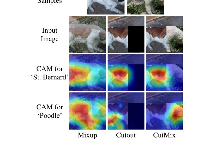
Figure 1: Class activation mapping (CAM) [52] visualizations on ‘Saint Bernard’ and ‘Miniature Poodle’ samples using various augmentation techniques. From top to bottom rows, we show the original images, input augmented image, CAM for class ‘Saint Bernard’, and CAM for class ‘Miniature Poodle’, respectively. Note that CutMix can take advantage of the mixed region on image, but Cutout cannot.

图 1：在 ImageNet 验证集「圣伯纳犬」与「迷你贵宾犬」上的类激活映射（CAM） [52] 可视化。CutMix 使模型准确定位两类物体，而 Cutout 聚焦于较少判别部位，Mixup 的激活较分散。

	Mixup	Cutout	CutMix
Usage of full image region	✔	✘	✔
Regional dropout	✘	✔	✔
Mixed image & label	✔	✘	✔

Table 2: Comparison among Mixup, Cutout, and CutMix.

	Mixup	Cutout	CutMix
Usage of full image region	✔	✘	✔
Regional dropout	✘	✔	✔
Mixed image & label	✔	✘	✔

表 2：Mixup、Cutout 与 CutMix 的性质对比。

We observe that Cutout successfully lets a model focus on less discriminative parts of the object, such as the belly of Saint Bernard, while being inefficient due to unused pixels. Mixup, on the other hand, makes full use of pixels, but introduces unnatural artifacts. The CAM for Mixup, as a result, shows that the model is confused when choosing cues for recognition. We hypothesize that such confusion leads to its suboptimal performance in classification and localization, as we will see in Section 4.

我们观察到：Cutout 成功让模型关注物体上较少判别的部位，例如犬身而非头部；但被遮挡区域不贡献学习信号。Mixup 因全局插值，激活往往分散且不自然。

CutMix efficiently improves upon Cutout by being able to localize the two object classes accurately. We summarize the key differences among Mixup, Cutout, and CutMix in Table 2.

CutMix 在 Cutout 基础上高效改进，能准确定位两个物体类别，同时充分利用全部像素。

Analysis on validation error: We analyze the effect of CutMix on stabilizing the training of deep networks. We compare the top-1 validation error during the training with CutMix against the baseline. We train ResNet-50 [12] for ImageNet Classification, and PyramidNet-200 [11] for CIFAR-100 Classification. Figure 2 shows the results.

验证误差分析： 我们分析 CutMix 对稳定深度网络训练的影响。图 2 给出 CIFAR-100 与 ImageNet 上的 top-1 测试误差曲线。

We observe, first of all, that CutMix achieves lower validation errors than the baseline at the end of training. At epoch 150 when the learning rates are reduced, the baselines suffer from overfitting with increasing validation error. CutMix, on the other hand, shows a steady decrease in validation error; diverse training samples reduce overfitting.

首先观察到，训练结束时 CutMix 的验证误差低于基线。其次，CutMix 缓解过拟合：基线在后期验证误差上升，而 CutMix 保持下降或平稳。这说明 CutMix 作为强正则化有效。

4 Experiments

4 实验

In this section, we evaluate CutMix for its capability to improve localizability as well as generalizability of a trained model on multiple tasks. We first study the effect of CutMix on image classification (Section 4.1) and weakly supervised object localization (Section 4.2). Next, we show the transferability of a CutMix pre-trained model when it is fine-tuned for object detection and image captioning tasks (Section 4.3). We also show that CutMix can improve the model robustness and alleviate the model over-confidence in Section 4.4.

本节评估 CutMix 提升可定位性与泛化能力的效果。我们先研究 CutMix 对图像分类（第 4.1 节）与弱监督目标定位（第 4.2 节）的影响；接着展示 CutMix 预训练模型微调到目标检测与图像描述时的迁移性（第 4.3 节）；并在第 4.4 节说明 CutMix 可提升鲁棒性、缓解过度自信。

All experiments were implemented and evaluated on NAVER Smart Machine Learning (NSML) [19] platform with PyTorch [29]. Source code and pretrained models are available at https://github.com/clovaai/CutMix-PyTorch.

全部实验在 NAVER Smart Machine Learning（NSML） [19] 平台用 PyTorch [29] 实现并评估。源代码与预训练模型见 https://github.com/clovaai/CutMix-PyTorch。

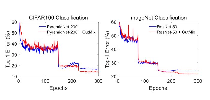
Figure 2: Top-1 test error plot for CIFAR100 (left) and ImageNet (right) classification. Cutmix achieves lower test errors than the baseline at the end of training.

图 2：CIFAR100（左）与 ImageNet（右）分类的 top-1 测试误差曲线。训练结束时 CutMix 的测试误差低于基线。

4.1 Image Classification

4.1 图像分类

4.1.1 ImageNet Classification

We evaluate on ImageNet-1K benchmark [31], the dataset containing 1.2M training images and 50K validation images of 1K categories. For fair comparison, we use the standard augmentation setting for ImageNet dataset such as re-sizing, cropping, and flipping, as done in [11, 8, 16, 37]. We found that regularization methods including Stochastic Depth [17], Cutout [3], Mixup [48], and CutMix require a greater number of training epochs till convergence. Therefore, we have trained all the models for $300$ epochs with initial learning rate $0.1$ decayed by factor $0.1$ at epochs $75$, $150$, and $225$. The batch size is set to $256$. The hyper-parameter $\alpha$ is set to $1$. We report the best performances of CutMix and other baselines during training.

4.1.1 ImageNet 分类

我们在 ImageNet-1K 基准 [31] 上评估，该数据集含 120 万训练图像与 5 万验证图像、1000 类。为公平比较，采用与 [11, 8, 16, 37] 相同的标准增强：缩放、裁剪与翻转。我们发现含 Stochastic Depth [17]、Cutout [3]、Mixup [48] 与 CutMix 在内的正则化方法需要更多 epoch 才能收敛，因此所有模型均训练 $300$ 个 epoch，初始学习率 $0.1$，在第 $75$、$150$、$225$ 个 epoch 乘以 $0.1$。批量大小 $256$，超参 $\alpha=1$。报告训练过程中 CutMix 与各基线的最佳表现。

Model	# Params	Top-1 Err (%)	Top-5 Err (%)
ResNet-152*	60.3 M	21.69	5.94
ResNet-101 + SE Layer* [15]	49.4 M	20.94	5.50
ResNet-101 + GE Layer* [14]	58.4 M	20.74	5.29
ResNet-50 + SE Layer* [15]	28.1 M	22.12	5.99
ResNet-50 + GE Layer* [14]	33.7 M	21.88	5.80
ResNet-50 (Baseline)	25.6 M	23.68	7.05
ResNet-50 + Cutout [3]	25.6 M	22.93	6.66
ResNet-50 + StochDepth [17]	25.6 M	22.46	6.27
ResNet-50 + Mixup [48]	25.6 M	22.58	6.40
ResNet-50 + Manifold Mixup [42]	25.6 M	22.50	6.21
ResNet-50 + DropBlock* [8]	25.6 M	21.87	5.98
ResNet-50 + Feature CutMix	25.6 M	21.80	6.06
ResNet-50 + CutMix	25.6 M	21.40	5.92

Table 3: ImageNet classification results based on ResNet-50 model. ‘*’ denotes results reported in the original papers.

Model	# Params	Top-1 Err (%)	Top-5 Err (%)
ResNet-152*	60.3 M	21.69	5.94
ResNet-101 + SE Layer* [15]	49.4 M	20.94	5.50
ResNet-101 + GE Layer* [14]	58.4 M	20.74	5.29
ResNet-50 + SE Layer* [15]	28.1 M	22.12	5.99
ResNet-50 + GE Layer* [14]	33.7 M	21.88	5.80
ResNet-50 (Baseline)	25.6 M	23.68	7.05
ResNet-50 + Cutout [3]	25.6 M	22.93	6.66
ResNet-50 + StochDepth [17]	25.6 M	22.46	6.27
ResNet-50 + Mixup [48]	25.6 M	22.58	6.40
ResNet-50 + Manifold Mixup [42]	25.6 M	22.50	6.21
ResNet-50 + DropBlock* [8]	25.6 M	21.87	5.98
ResNet-50 + Feature CutMix	25.6 M	21.80	6.06
ResNet-50 + CutMix	25.6 M	21.40	5.92

表 3：ImageNet 分类结果。CutMix 在所比较的增强策略中取得最佳 top-1 / top-5。

We briefly describe the settings for baseline augmentation schemes. We set the dropping rate of residual blocks to $0.25$ for the best performance of Stochastic Depth [17]. The mask size for Cutout [3] is set to $112\times 112$ and the location for dropping out is uniformly sampled. The performance of DropBlock [8] is from the original paper and the difference from our setting is the training epochs which is set to $270$. Manifold Mixup [42] applies Mixup operation on the randomly chosen internal feature map. We have tried $\alpha=0.5$ and $1.0$ for Mixup and Manifold Mixup and have chosen $1.0$ which has shown better performances. It is also possible to extend CutMix to feature-level augmentation (Feature CutMix). Feature CutMix applies CutMix at a randomly chosen layer per minibatch as Manifold Mixup does.

下面简述基线增强方案设置。Stochastic Depth [17] 残差块丢弃率设为 $0.25$ 以取得最佳表现。Cutout [3] 掩码大小设为 $112\times 112$，丢弃位置均匀采样。DropBlock [8] 结果取自原文，与我们设置的差异在于训练 epoch 为 $270$。Manifold Mixup [42] 在随机选择的内部特征图上做 Mixup。我们对 Mixup 与 Manifold Mixup 尝试了 $\alpha=0.5$ 与 $1.0$，并选用表现更好的 $1.0$。也可将 CutMix 扩展到特征级增强（Feature CutMix），像 Manifold Mixup 一样在每个小批量随机选择一层施加 CutMix。

Model	# Params	Top-1 Err (%)	Top-5 Err (%)
ResNet-101 (Baseline) [12]	44.6 M	21.87	6.29
ResNet-101 + Cutout [3]	44.6 M	20.72	5.51
ResNet-101 + Mixup [48]	44.6 M	20.52	5.28
ResNet-101 + CutMix	44.6 M	20.17	5.24
ResNeXt-101 (Baseline) [45]	44.1 M	21.18	5.57
ResNeXt-101 + CutMix	44.1 M	19.47	5.03

Table 4: Impact of CutMix on ImageNet classification for ResNet-101 and ResNext-101.

Model	# Params	Top-1 Err (%)	Top-5 Err (%)
ResNet-101 (Baseline) [12]	44.6 M	21.87	6.29
ResNet-101 + Cutout [3]	44.6 M	20.72	5.51
ResNet-101 + Mixup [48]	44.6 M	20.52	5.28
ResNet-101 + CutMix	44.6 M	20.17	5.24
ResNeXt-101 (Baseline) [45]	44.1 M	21.18	5.57
ResNeXt-101 + CutMix	44.1 M	19.47	5.03

表 4：CutMix 对更深网络 ImageNet 分类的影响。

Comparison against baseline augmentations: Results are given in Table 3. We observe that CutMix achieves the best result, 21.40% top-1 error, among the considered augmentation strategies. CutMix outperforms Cutout and Mixup, the two closest approaches to ours, by $+1.53\%$ and $+1.18\%$, respectively. On the feature level as well, we find CutMix preferable to Mixup, with top-1 errors $21.78\%$ and $22.50\%$, respectively.

与基线增强比较： 结果见表 3。CutMix 在所比较的增强策略中取得最佳结果，top-1 误差 21.40%。相对最接近的 Cutout 与 Mixup，分别提升 $+1.53\%$ 与 $+1.18\%$。在特征级上，CutMix 也优于 Mixup，top-1 误差分别为 $21.78\%$ 与 $22.50\%$。

Comparison against architectural improvements: We have also compared improvements due to CutMix versus architectural improvements (e.g. greater depth or additional modules). We observe that CutMix improves the performance by +2.28% while increased depth (ResNet-50 $\rightarrow$ ResNet-152) boosts $+1.99\%$ and SE [15] and GE [14] boosts $+1.56\%$ and $+1.80\%$, respectively. Note that unlike above architectural boosts improvements due to CutMix come at little or memory or computational time.

与架构改进比较： 我们还将 CutMix 带来的提升与架构改进（如更深网络或额外模块）比较。CutMix 提升 +2.28%，而加深（ResNet-50 $\rightarrow$ ResNet-152）提升 $+1.99\%$，SE [15] 与 GE [14] 分别提升 $+1.56\%$ 与 $+1.80\%$。注意与上述架构提升不同，CutMix 几乎不增加显存或计算时间。

CutMix for Deeper Models: We have explored the performance of CutMix for the deeper networks, ResNet-101 [12] and ResNeXt-101 (32$\times$4d) [45], on ImageNet. As seen in Table 4, we observe +1.60% and +1.71% respective improvements in top-1 errors due to CutMix.

更深模型上的 CutMix： 我们在 ImageNet 上考察了更深网络 ResNet-101 [12] 与 ResNeXt-101（$32\times 4$d） [45]。如表 4，CutMix 分别带来 +1.60% 与 +1.71% 的 top-1 误差改善。

4.1.2 CIFAR Classification

We set mini-batch size to $64$ and training epochs to $300$. The learning rate was initially set to $0.25$ and decayed by the factor of $0.1$ at $150$ and $225$ epoch. To ensure the effectiveness of the proposed method, we used a strong baseline, PyramidNet-200 [11] with widening factor $\tilde{\alpha}=240$. It has $26.8$M parameters and achieves the state-of-the-art performance $16.45\%$ top-1 error on CIFAR-100.

4.1.2 CIFAR 分类

小批量设为 $64$，训练 $300$ 个 epoch。初始学习率 $0.25$，在第 $150$ 与 $225$ 个 epoch 乘以 $0.1$。为确保方法有效，我们使用强基线 PyramidNet-200 [11]（加宽因子 $\tilde{\alpha}=240$），参数量 $26.8$M，在 CIFAR-100 上达到当时最优 $16.45\%$ top-1 误差。

PyramidNet-200 ($\tilde{\alpha}$=240) (# params: 26.8 M)	Top-1 Err (%)	Top-5 Err (%)
Baseline	16.45	3.69
+ StochDepth [17]	15.86	3.33
+ Label smoothing ($\epsilon$=0.1) [38]	16.73	3.37
+ Cutout [3]	16.53	3.65
+ Cutout + Label smoothing ($\epsilon$=0.1)	15.61	3.88
+ DropBlock [8]	15.73	3.26
+ DropBlock + Label smoothing ($\epsilon$=0.1)	15.16	3.86
+ Mixup ($\alpha$=0.5) [48]	15.78	4.04
+ Mixup ($\alpha$=1.0) [48]	15.63	3.99
+ Manifold Mixup ($\alpha$=1.0) [42]	16.14	4.07
+ Cutout + Mixup ($\alpha$=1.0)	15.46	3.42
+ Cutout + Manifold Mixup ($\alpha$=1.0)	15.09	3.35
+ ShakeDrop [46]	15.08	2.72
+ CutMix	14.47	2.97
+ CutMix + ShakeDrop [46]	13.81	2.29

Table 5: Comparison of state-of-the-art regularization methods on CIFAR-100.

PyramidNet-200 ($\tilde{\alpha}$=240) (# params: 26.8 M)	Top-1 Err (%)	Top-5 Err (%)
Baseline	16.45	3.69
+ StochDepth [17]	15.86	3.33
+ Label smoothing ($\epsilon$=0.1) [38]	16.73	3.37
+ Cutout [3]	16.53	3.65
+ Cutout + Label smoothing ($\epsilon$=0.1)	15.61	3.88
+ DropBlock [8]	15.73	3.26
+ DropBlock + Label smoothing ($\epsilon$=0.1)	15.16	3.86
+ Mixup ($\alpha$=0.5) [48]	15.78	4.04
+ Mixup ($\alpha$=1.0) [48]	15.63	3.99
+ Manifold Mixup ($\alpha$=1.0) [42]	16.14	4.07
+ Cutout + Mixup ($\alpha$=1.0)	15.46	3.42
+ Cutout + Manifold Mixup ($\alpha$=1.0)	15.09	3.35
+ ShakeDrop [46]	15.08	2.72
+ CutMix	14.47	2.97
+ CutMix + ShakeDrop [46]	13.81	2.29

表 5：在 PyramidNet-200 上与其他数据增强与正则化方法的 CIFAR-100 比较。

Table 5 shows the performance comparison against other state-of-the-art data augmentation and regularization methods. All experiments were conducted three times and the averaged best performances during training are reported.

表 5 给出与其他当时最优数据增强与正则化方法的比较。全部实验重复三次，报告训练过程中平均最佳表现。

Hyper-parameter settings: We set the hole size of Cutout [3] to $16\times 16$. For DropBlock [8], keep_prob and block_size are set to $0.9$ and $4$, respectively. The drop rate for Stochastic Depth [17] is set to 0.25. For Mixup [48], we tested the hyper-parameter $\alpha$ with 0.5 and 1.0. For Manifold Mixup [42], we applied Mixup operation at a randomly chosen layer per minibatch.

超参设置： Cutout [3] 的孔洞大小设为 $16\times 16$。DropBlock [8] 的 keep_prob 与 block_size 分别为 $0.9$ 与 $4$。Stochastic Depth [17] 丢弃率 $0.25$。Mixup [48] 测试了 $\alpha=0.5$ 与 $1.0$。Manifold Mixup [42] 在每个小批量随机选择一层施加 Mixup。

Model	# Params	Top-1 Err (%)	Top-5 Err (%)
PyramidNet-110 ($\tilde{\alpha}=64$) [11]	1.7 M	19.85	4.66
PyramidNet-110 + CutMix	1.7 M	17.97	3.83
ResNet-110 [12]	1.1 M	23.14	5.95
ResNet-110 + CutMix	1.1 M	20.11	4.43

Table 6: Impact of CutMix on lighter architectures on CIFAR-100.

Model	# Params	Top-1 Err (%)	Top-5 Err (%)
PyramidNet-110 ($\tilde{\alpha}=64$) [11]	1.7 M	19.85	4.66
PyramidNet-110 + CutMix	1.7 M	17.97	3.83
ResNet-110 [12]	1.1 M	23.14	5.95
ResNet-110 + CutMix	1.1 M	20.11	4.43

表 6：CutMix 对较弱基线架构 CIFAR-100 分类的影响。

PyramidNet-200 ($\tilde{\alpha}$=240)	Top-1 Error (%)
Baseline	3.85
+ Cutout	3.10
+ Mixup ($\alpha$=1.0)	3.09
+ Manifold Mixup ($\alpha$=1.0)	3.15
+ CutMix	2.88

Table 7: Impact of CutMix on CIFAR-10.

PyramidNet-200 ($\tilde{\alpha}$=240)	Top-1 Error (%)
Baseline	3.85
+ Cutout	3.10
+ Mixup ($\alpha$=1.0)	3.09
+ Manifold Mixup ($\alpha$=1.0)	3.15
+ CutMix	2.88

表 7：CutMix 在 CIFAR-10 上的影响。

Combination of regularization methods: We have evaluated the combination of regularization methods. Both Cutout [3] and label smoothing [38] does not improve the accuracy when adopted independently, but they are effective when used together. Dropblock [8], the feature-level generalization of Cutout, is also more effective when label smoothing is also used. Mixup [48] and Manifold Mixup [42] achieve higher accuracies when Cutout is applied on input images. The combination of Cutout and Mixup tends to generate locally separated and mixed samples since the cropped regions have less ambiguity than those of the vanilla Mixup. The superior performance of Cutout and Mixup combination shows that mixing via cut-and-paste manner is better than interpolation, as much evidenced by CutMix performances.

正则化方法组合： 我们评估了正则化方法的组合。Cutout [3] 与标签平滑 [38] 单独使用时并不提升精度，但一起用时有效。Cutout 的特征级推广 DropBlock [8] 在配合标签平滑时也更有效。Mixup [48] 与 Manifold Mixup [42] 在输入图像上再加 Cutout 时精度更高。Cutout 与 Mixup 的组合倾向于生成局部可分且混合的样本，因为裁剪区域比原版 Mixup 更少歧义。Cutout+Mixup 的优越表现说明剪切粘贴式混合优于插值，这也被 CutMix 的表现所印证。

CutMix achieves $14.47\%$ top-1 classification error on CIFAR-100, $+1.98\%$ higher than the baseline performance $16.45\%$. We have achieved a new state-of-the-art performance $13.81\%$ by combining CutMix and ShakeDrop [46], a regularization that adds noise on intermediate features.

CutMix 在 CIFAR-100 上达到 $14.47\%$ top-1 分类误差，相对基线 $16.45\%$ 提升 $+1.98\%$。将 CutMix 与在中间特征上加噪声的 ShakeDrop [46] 结合，我们取得新的当时最优 $13.81\%$。

CutMix for various models: Table 6 shows CutMix also significantly improves the performance of the weaker baseline architectures, such as PyramidNet-110 [11] and ResNet-110.

多种模型上的 CutMix： 表 6 显示，CutMix 同样显著提升较弱基线架构（如 PyramidNet-110 [11] 与 ResNet-110）的表现。

CutMix for CIFAR-10: We have evaluated CutMix on CIFAR-10 dataset using the same baseline and training setting for CIFAR-100. The results are given in Table 7. On CIFAR-10, CutMix also enhances the classification performances by $+0.97\%$, outperforming Mixup and Cutout performances.

CIFAR-10 上的 CutMix： 我们用与 CIFAR-100 相同的基线与训练设置在 CIFAR-10 上评估。结果见表 7。在 CIFAR-10 上 CutMix 也将分类表现提升 $+0.97\%$，优于 Mixup 与 Cutout。

4.1.3 Ablation Studies

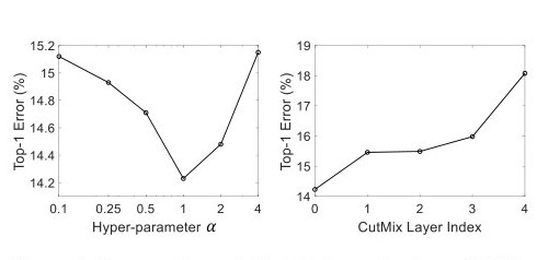
Figure 3: Impact of $\alpha$ and CutMix layer depth on CIFAR-100 top-1 error.

4.1.3 消融实验

图 3：$\alpha$ 与 CutMix 作用层深度对 CIFAR-100 top-1 误差的影响。

We conducted ablation study in CIFAR-100 dataset using the same experimental settings in Section 4.1.2. We evaluated CutMix with $\alpha\in\{0.1,0.25,0.5,1.0,2.0,4.0\}$; the results are given in Figure 3, left plot. For all $\alpha$ values considered, CutMix improves upon the baseline ($16.45\%$). The best performance is achieved when $\alpha=1.0$.

我们在 CIFAR-100 上用第 4.1.2 节相同实验设置做消融。评估 $\alpha\in\{0.1,0.25,0.5,1.0,2.0,4.0\}$；结果见图 3 左图。对所有考虑的 $\alpha$，CutMix 都优于基线（$16.45\%$）。最佳表现为 $\alpha=1.0$。

The performance of feature-level CutMix is given in Figure 3, right plot. We changed the layer on which CutMix is applied, from image layer itself to higher feature levels. We denote the index as (0=image level, 1=after first conv-bn, 2=after layer1, 3=after layer2, 4=after layer3). CutMix achieves the best performance when it is applied on the input images. Again, feature-level CutMix except the layer3 case improves the accuracy over the baseline ($16.45\%$).

特征级 CutMix 的表现见图 3 右图。我们改变施加 CutMix 的层，从图像层本身到更高特征层。索引记为（0=图像级，1=第一个 conv-bn 之后，2=layer1 之后，3=layer2 之后，4=layer3 之后）。CutMix 在输入图像上施加时表现最佳。除 layer3 外，特征级 CutMix 也都优于基线（$16.45\%$）。

PyramidNet-200 ($\tilde{\alpha}$=240) ($\#$ params: 26.8 M)	Top-1 Error (%)	Top-5 Error (%)
Baseline	16.45	3.69
Proposed (CutMix)	14.47	2.97
Center Gaussian CutMix	15.95	3.40
Fixed-size CutMix	14.97	3.15
One-hot CutMix	15.89	3.32
Scheduled CutMix	14.72	3.17
Complete-label CutMix	15.17	3.10

Table 8: Performance of CutMix variants on CIFAR-100.

PyramidNet-200 ($\tilde{\alpha}$=240) ($\#$ params: 26.8 M)	Top-1 Error (%)	Top-5 Error (%)
Baseline	16.45	3.69
Proposed (CutMix)	14.47	2.97
Center Gaussian CutMix	15.95	3.40
Fixed-size CutMix	14.97	3.15
One-hot CutMix	15.89	3.32
Scheduled CutMix	14.72	3.17
Complete-label CutMix	15.17	3.10

表 8：CutMix 设计变体在 CIFAR-100 上的表现。

We explore different design choices for CutMix. Table 8 shows the performance of CutMix variations. ‘Center Gaussian CutMix’ samples the box coordinates $r_{x},r_{y}$ of Equation (2) according to the Gaussian distribution with mean at the image center, instead of the original uniform distribution. ‘Fixed-size CutMix’ fixes the size of cropping region $(r_{w},r_{h})$ at $16\times 16$ (i.e. $\lambda=0.75$). ‘Scheduled CutMix’ linearly increases the probability to apply CutMix as training progresses, as done by [8, 17], from $0$ to $1$. ‘One-hot CutMix’ decides the mixed target label by committing to the label of greater patch portion (single one-hot label), rather than using the combination strategy in Equation (1). ‘Complete-label CutMix’ assigns the mixed target label as $\tilde{y}=0.5y_{A}+0.5y_{B}$ regardless of the combination ratio $\lambda$. The results show that above variations lead to performance degradation compared to the original CutMix.

我们探索 CutMix 的不同设计选择。表 8 给出各变体表现。「Center Gaussian CutMix」按以图像中心为均值的高斯分布采样公式 (2) 的盒坐标 $r_{x},r_{y}$，而非原来的均匀分布。「Fixed-size CutMix」把裁剪区域大小 $(r_{w},r_{h})$ 固定为 $16\times 16$（即 $\lambda=0.75$）。「Scheduled CutMix」随训练进程把施加 CutMix 的概率从 $0$ 线性增至 $1$，如 [8, 17]。「One-hot CutMix」按较大补丁占比的标签做 one-hot，而非公式 (1) 的组合策略。「Complete-label CutMix」不论组合比 $\lambda$ 如何，都将混合标签设为 $\tilde{y}=0.5y_{A}+0.5y_{B}$。结果表明上述变体相对原版 CutMix 都会造成表现下降。

4.2 Weakly Supervised Object Localization

4.2 弱监督目标定位

Method	CUB200-2011 Loc Acc (%)	CUB200-2011	Loc Acc (%)	ImageNet Loc Acc (%)	ImageNet	Loc Acc (%)
CUB200-2011
Loc Acc (%)
ImageNet
Loc Acc (%)
VGG-GAP + CAM [52]	37.12	42.73
VGG-GAP + ACoL* [49]	45.92	45.83
VGG-GAP + ADL* [2]	52.36	44.92
GoogLeNet + HaS* [33]	-	45.21
InceptionV3 + SPG* [50]	46.64	48.60
VGG-GAP + Mixup [48]	41.73	42.54
VGG-GAP + Cutout [3]	44.83	43.13
VGG-GAP + CutMix	52.53	43.45
ResNet-50 + CAM [52]	49.41	46.30
ResNet-50 + Mixup [48]	49.30	45.84
ResNet-50 + Cutout [3]	52.78	46.69
ResNet-50 + CutMix	54.81	47.25

CUB200-2011
Loc Acc (%)

ImageNet
Loc Acc (%)

Table 9: Weakly supervised object localization results on CUB200-2011 and ImageNet. * denotes results reported in the original papers.

Method	CUB200-2011 Loc Acc (%)	CUB200-2011	Loc Acc (%)	ImageNet Loc Acc (%)	ImageNet	Loc Acc (%)
CUB200-2011
Loc Acc (%)
ImageNet
Loc Acc (%)
VGG-GAP + CAM [52]	37.12	42.73
VGG-GAP + ACoL* [49]	45.92	45.83
VGG-GAP + ADL* [2]	52.36	44.92
GoogLeNet + HaS* [33]	-	45.21
InceptionV3 + SPG* [50]	46.64	48.60
VGG-GAP + Mixup [48]	41.73	42.54
VGG-GAP + Cutout [3]	44.83	43.13
VGG-GAP + CutMix	52.53	43.45
ResNet-50 + CAM [52]	49.41	46.30
ResNet-50 + Mixup [48]	49.30	45.84
ResNet-50 + Cutout [3]	52.78	46.69
ResNet-50 + CutMix	54.81	47.25

CUB200-2011
Loc Acc (%)

ImageNet
Loc Acc (%)

表 9：弱监督目标定位结果。CutMix 在 CUB200-2011 与 ImageNet 上均提升定位精度。

Backbone Network	ImageNet Cls Top-1 Error (%)	Detection	Image Captioning
SSD [24] (mAP)	Faster-RCNN [30] (mAP)	NIC [43] (BLEU-1)	NIC [43] (BLEU-4)
ResNet-50 (Baseline)	23.68	76.7 (+0.0)	75.6 (+0.0)	61.4 (+0.0)	22.9 (+0.0)
Mixup-trained	22.58	76.6 (-0.1)	73.9 (-1.7)	61.6 (+0.2)	23.2 (+0.3)
Cutout-trained	22.93	76.8 (+0.1)	75.0 (-0.6)	63.0 (+1.6)	24.0 (+1.1)
CutMix-trained	21.40	77.6 (+0.9)	76.7 (+1.1)	64.2 (+2.8)	24.9 (+2.0)

Table 10: Impact of CutMix on transfer learning of pretrained model to other tasks, object detection and image captioning.

Backbone Network	ImageNet Cls Top-1 Error (%)	Detection	Image Captioning
SSD [24] (mAP)	Faster-RCNN [30] (mAP)	NIC [43] (BLEU-1)	NIC [43] (BLEU-4)
ResNet-50 (Baseline)	23.68	76.7 (+0.0)	75.6 (+0.0)	61.4 (+0.0)	22.9 (+0.0)
Mixup-trained	22.58	76.6 (-0.1)	73.9 (-1.7)	61.6 (+0.2)	23.2 (+0.3)
Cutout-trained	22.93	76.8 (+0.1)	75.0 (-0.6)	63.0 (+1.6)	24.0 (+1.1)
CutMix-trained	21.40	77.6 (+0.9)	76.7 (+1.1)	64.2 (+2.8)	24.9 (+2.0)

表 10：CutMix 对迁移学习的影响：Pascal VOC 检测与 MS-COCO 图像描述。

Weakly supervised object localization (WSOL) task aims to train the classifier to localize target objects by using only the class labels. To localize the target well, it is important to make CNNs extract cues from full object regions and not focus on small discriminant parts of the target. Learning spatially distributed representation is thus the key for improving performance on WSOL task. CutMix guides a classifier to attend to broader sets of cues to make decisions; we expect CutMix to improve WSOL performances of classifiers. To measure this, we apply CutMix over baseline WSOL models. We followed the training and evaluation strategy of existing WSOL methods [49, 50, 2] with VGG-GAP and ResNet-50 as the base architectures. The quantitative and qualitative results are given in Table 9 and Figure 4, respectively. Full implementation details are in Appendix B.

弱监督目标定位（WSOL）任务旨在仅用类别标签训练分类器以定位目标物体。要定得好，关键是让 CNN 从物体完整区域提取线索，而不是只盯判别性小部位。学习空间上分散的表征因此是提升 WSOL 的关键。CutMix 引导分类器关注更广的线索集合；我们预期它能改善分类器的 WSOL 表现。为此，我们在基线 WSOL 模型上施加 CutMix，并在 CUB200-2011 与 ImageNet 上评估。

Comparison against Mixup and Cutout: CutMix outperforms Mixup [48] on localization accuracies by $+5.51\%$ and $+1.41\%$ on CUB200-2011 and ImageNet, respectively. Mixup degrades the localization accuracy of the baseline model; it tends to make a classifier focus on small regions as shown in Figure 4. As we have hypothesized in Section 3.2, more ambiguity in Mixup samples make a classifier focus on even more discriminative parts of objects, leading to decreased localization accuracies. Although Cutout [3] improves the accuracy over the baseline, it is outperformed by CutMix: $+2.03\%$ and $+0.56\%$ on CUB200-2011 and ImageNet, respectively.

与 Mixup、Cutout 比较： CutMix 在 CUB200-2011 与 ImageNet 上的定位精度分别比 Mixup [48] 高 $+5.51\%$ 与 $+1.41\%$。Mixup 反而降低基线定位精度；如图 4 所示，它倾向于让分类器聚焦更小区域。如第 3.2 节所假设，Mixup 样本中更大的歧义会使分类器更盯物体判别部位，从而降低定位精度。Cutout [3] 虽优于基线，但仍逊于 CutMix。

CutMix also achieves comparable localization accuracies on CUB200-2011 and ImageNet, even when compared against the dedicated state-of-the-art WSOL methods [52, 33, 49, 50, 2] that focus on learning spatially dispersed representations.

即便与专注学习空间分散表征的专用当时最优 WSOL 方法 [52, 33, 49, 50, 2] 相比，CutMix 在 CUB200-2011 与 ImageNet 上也取得可比的定位精度。

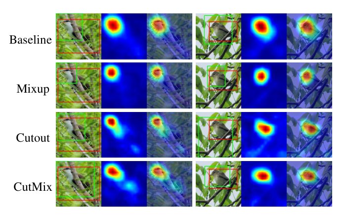
Figure 4: Qualitative comparison of the baseline (ResNet-50), Mixup, Cutout, and CutMix for weakly supervised object localization task on CUB-200-2011 dataset. Ground truth and predicted bounding boxes are denoted as red and green, respectively.

图 4：基线（ResNet-50）、Mixup、Cutout 与 CutMix 在 CUB-200-2011 弱监督目标定位上的定性比较。真实框与预测框分别用红、绿表示。

4.3 Transfer Learning of Pretrained Model

4.3 预训练模型的迁移学习

ImageNet pre-training is de-facto standard practice for many visual recognition tasks. We examine whether CutMix pre-trained models leads to better performances in certain downstream tasks based on ImageNet pre-trained models. As CutMix has shown superiority in localizing less discriminative object parts, we would expect it to lead to boosts in certain recognition tasks with localization elements, such as object detection and image captioning. We evaluate the boost from CutMix on those tasks by replacing the backbone network initialization with other ImageNet pre-trained models using Mixup [48], Cutout [3], and CutMix. ResNet-50 is used as the baseline architecture in this section.

ImageNet 预训练是许多视觉识别任务的事实标准。我们考察 CutMix 预训练模型在依赖 ImageNet 预训练的下游任务上是否更好。由于 CutMix 在定位较少判别的物体部位上表现更强，我们预期它会在带定位要素的识别任务（如目标检测与图像描述）上带来提升。通过把骨干初始化替换为 Mixup、Cutout 或 CutMix 的 ImageNet 预训练模型，我们评估这种提升。

Transferring to Pascal VOC object detection: Two popular detection models, SSD [24] and Faster RCNN [30], are considered. Originally the two methods have utilized VGG-16 as backbones, but we have changed it to ResNet-50. The ResNet-50 backbone is initialized with various ImageNet-pretrained models and then fine-tuned on Pascal VOC 2007 and 2012 [6] trainval data. Models are evaluated on VOC 2007 test data using the mAP metric. We follow the fine-tuning strategy of the original methods [24, 30]; implementation details are in Appendix C. Results are shown in Table 10. Pre-training with Cutout and Mixup has failed to improve the object detection performance over the vanilla pre-trained model. However, the pre-training with CutMix improves the performance of both SSD and Faster-RCNN. Stronger localizability of the CutMix pre-trained models leads to better detection performances.

迁移到 Pascal VOC 目标检测： 考虑两种流行检测模型 SSD [24] 与 Faster R-CNN [30]。二者原用 VGG-16 作骨干，我们改为 ResNet-50。ResNet-50 骨干用多种 ImageNet 预训练模型初始化，再在 Pascal VOC 2007 与 2012 [6] trainval 上微调，于 VOC 2007 test 上用 mAP 评估。微调策略遵循原文 [24, 30]；实现细节见附录 C。结果见表 10。CutMix 预训练在两种检测器上都带来稳定增益。

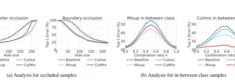
(a) Analysis for occluded samples

(a) 遮挡样本分析

Transferring to MS-COCO image captioning: We used Neural Image Caption (NIC) [43] as the base model for image captioning experiments. We have changed the backbone network of encoder from GoogLeNet [43] to ResNet-50. The backbone network is initialized with various ImageNet pre-trained models, and then trained and evaluated on MS-COCO dataset [23]. Implementation details and evaluation metrics (METEOR, CIDER, etc.) are in Appendix D. Table 10 shows the results. CutMix outperforms Mixup and Cutout in both BLEU1 and BLEU4 metrics. Simply replacing backbone network with our CutMix pre-trained model gives performance gains for object detection and image captioning tasks at no extra cost.

迁移到 MS-COCO 图像描述： 以 Neural Image Caption（NIC） [43] 为基模型。编码器骨干由 GoogLeNet [43] 改为 ResNet-50，用多种 ImageNet 预训练模型初始化，再在 MS-COCO [23] 上训练与评估。实现细节与指标（METEOR、CIDEr 等）见附录 D。表 10 显示：CutMix 在 BLEU1 与 BLEU4 上均优于 Mixup 与 Cutout。仅把骨干换成 CutMix 预训练即可稳定提升描述质量。

4.4 Robustness and Uncertainty

4.4 鲁棒性与不确定性

Many researches have shown that deep models are easily fooled by small and unrecognizable perturbations on the input images, a phenomenon referred to as adversarial attacks [9, 39]. One straightforward way to enhance robustness and uncertainty is an input augmentation by generating unseen samples [26]. We evaluate robustness and uncertainty improvements due to input augmentation methods including Mixup, Cutout, and CutMix.

大量研究表明，深度模型易被输入上微小且难以察觉的扰动愚弄，即对抗攻击 [9, 39]。增强鲁棒性与不确定性的一条直接路径是通过生成未见样本做输入增强 [26]。我们评估 Mixup、Cutout 与 CutMix 等输入增强对鲁棒性与不确定性的改善。

Robustness: We evaluate the robustness of the trained models to adversarial samples, occluded samples, and in-between class samples. We use ImageNet pre-trained ResNet-50 models with same setting as in Section 4.1.1.

鲁棒性： 评估训练模型对对抗样本、遮挡样本与类间插值样本的鲁棒性。使用与第 4.1.1 节相同设置的 ImageNet 预训练 ResNet-50。

Fast Gradient Sign Method (FGSM) [9] is used to generate adversarial perturbations and we assume that the adversary has full information of the models (white-box attack). We report top-1 accuracies after attack on ImageNet validation set in Table 11. CutMix significantly improves the robustness to adversarial attacks compared to other augmentation methods.

用快速梯度符号法（FGSM） [9] 生成对抗扰动，并假设攻击者掌握模型全部信息（白盒攻击）。ImageNet 验证集受攻击后的 top-1 精度见表 11。相对其他增强方法，CutMix 显著提升对抗鲁棒性。

For occlusion experiments, we generate occluded samples in two ways: center occlusion by filling zeros in a center hole and boundary occlusion by filling zeros outside of the hole. In Figure 6(a), we measure the top-1 error by varying the hole size from $0$ to $224$. For both occlusion scenarios, Cutout and CutMix achieve significant improvements in robustness while Mixup only marginally improves it. Interestingly, CutMix almost achieves a comparable performance as Cutout even though CutMix has not observed any occluded sample during training unlike Cutout.

遮挡实验中，我们以两种方式生成遮挡样本：中心遮挡（在中心孔洞填零）与边界遮挡（在孔洞外填零）。在图 5(a) 中，我们让孔洞大小从 $0$ 变到 $224$ 并测量 top-1 误差。两种遮挡场景下，Cutout 与 CutMix 都显著提升鲁棒性，而 Mixup 仅略有改善。有趣的是，尽管 CutMix 训练中从未见过遮挡样本（不像 Cutout），其表现几乎可与 Cutout 相比。

Finally, we evaluate the top-1 error of Mixup and CutMix in-between samples. The probability to predict neither two classes by varying the combination ratio $\lambda$ is illustrated in Figure 6(b). We randomly select $50,000$ in-between samples in ImageNet validation set. In both experiments, Mixup and CutMix improve the performance while improvements due to Cutout are almost negligible. Similarly to the previous occlusion experiments, CutMix even improves the robustness to the unseen Mixup in-between class samples.

最后，我们评估 Mixup 与 CutMix 类间插值样本上的 top-1 误差。随组合比 $\lambda$ 变化、预测为两类皆非的概率见图 5(b)。在 ImageNet 验证集上随机选取 $50{,}000$ 个类间样本。两组实验中 Mixup 与 CutMix 都改善表现，而 Cutout 几乎无增益。与遮挡实验类似，CutMix 甚至提升对未见过的 Mixup 类间样本的鲁棒性。

	Baseline	Mixup	Cutout	CutMix
Top-1 Acc (%)	8.2	24.4	11.5	31.0

Table 11: Top-1 accuracy after FGSM white-box attack on ImageNet validation set.

	Baseline	Mixup	Cutout	CutMix
Top-1 Acc (%)	8.2	24.4	11.5	31.0

表 11：ImageNet 验证集上 FGSM 白盒攻击后的 top-1 精度。

Method	TNR at TPR 95%	AUROC	Detection Acc.
Baseline	26.3 (+0)	87.3 (+0)	82.0 (+0)
Mixup	11.8 (-14.5)	49.3 (-38.0)	60.9 (-21.0)
Cutout	18.8 (-7.5)	68.7 (-18.6)	71.3 (-10.7)
CutMix	69.0 (+42.7)	94.4 (+7.1)	89.1 (+7.1)

Table 12: Out-of-distribution (OOD) detection results with CIFAR-100 trained models. Results are averaged on seven datasets. All numbers are in percents; higher is better.

Method	TNR at TPR 95%	AUROC	Detection Acc.
Baseline	26.3 (+0)	87.3 (+0)	82.0 (+0)
Mixup	11.8 (-14.5)	49.3 (-38.0)	60.9 (-21.0)
Cutout	18.8 (-7.5)	68.7 (-18.6)	71.3 (-10.7)
CutMix	69.0 (+42.7)	94.4 (+7.1)	89.1 (+7.1)

表 12：用 CIFAR-100 训练模型做分布外（OOD）检测的结果。七个数据集平均；数字为百分数，越高越好。

Uncertainty: We measure the performance of the out-of-distribution (OOD) detectors proposed by [13] which determines whether the sample is in- or out-of-distribution by score thresholding. We use PyramidNet-200 trained on CIFAR-100 datasets with same setting as in Section 4.1.2. In Table 12, we report the averaged OOD detection performances against seven out-of-distribution samples from [13, 22], including TinyImageNet, LSUN [47], uniform noise, Gaussian noise, etc. More results are illustrated in Appendix E. Mixup and Cutout augmentations aggravate the over-confidence of the base networks. Meanwhile, CutMix significantly alleviates the over-confidence of the model.

不确定性： 我们用 [13] 提出的分布外（OOD）检测器衡量表现，该检测器通过分数阈值判断样本是否在分布内。使用与第 4.1.2 节相同设置、在 CIFAR-100 上训练的 PyramidNet-200。表 12 报告相对 [13, 22] 中七种分布外样本（含 TinyImageNet、LSUN [47]、均匀噪声、高斯噪声等）的平均 OOD 检测表现。更多结果见附录 E。Mixup 与 Cutout 增强会加重基线网络的过度自信，而 CutMix 显著改善 OOD 检测。

5 Conclusion

5 结论

We have introduced CutMix for training CNNs with strong classification and localization ability. CutMix is easy to implement and has no computational overhead, while being surprisingly effective on various tasks. On ImageNet classification, applying CutMix to ResNet-50 and ResNet-101 brings $+2.28\%$ and $+1.70\%$ top-1 accuracy improvements. On CIFAR classification, CutMix significantly improves the performance of baseline by $+1.98\%$ leads to the state-of-the-art top-1 error $14.47\%$. On weakly supervised object localization (WSOL), CutMix substantially enhances the localization accuracy and has achieved comparable localization performances as the state-of-the-art WSOL methods. Furthermore, simply using CutMix-ImageNet-pretrained model as the initialized backbone of the object detection and image captioning brings overall performance improvements. Finally, we have shown that CutMix results in improvements in robustness and uncertainty of image classifiers over the vanilla model as well as other regularized models.

我们提出 CutMix，用于训练兼具强分类与定位能力的 CNN。CutMix 易于实现、几乎无计算开销，却在多种任务上出人意料地有效。在 ImageNet 分类上，对 ResNet-50 与 ResNet-101 施加 CutMix 分别带来 $+2.28\%$ 与 $+1.70\%$ 的 top-1 精度提升。在 CIFAR 分类上，CutMix 显著改进强基线并与其他正则化互补。CutMix 还提升弱监督定位，并把增益迁移到检测与图像描述。对鲁棒性与不确定性的分析进一步表明：CutMix 训练的模型对遮挡、对抗扰动与分布外输入更可靠。我们期望 CutMix 成为训练视觉识别模型的实用默认增强之一。

Acknowledgement

致谢

We would like to thank Clova AI Research team, especially Jung-Woo Ha and Ziad Al-Halah for their helpful feedback and discussion.

感谢 Clova AI Research 团队，尤其是 Jung-Woo Ha 与 Ziad Al-Halah 的有益讨论与支持。

References

参考文献

[1] Liang-Chieh Chen, George Papandreou, Iasonas Kokkinos, Kevin Murphy, and Alan L Yuille. Deeplab: Semantic image segmentation with deep convolutional nets, atrous convolution, and fully connected crfs. IEEE transactions on pattern analysis and machine intelligence , 40(4):834–848, 2018.

[2] Junsuk Choe and Hyunjung Shim. Attention-based dropout layer for weakly supervised object localization. In Proceedings of the IEEE Conference on Computer Vision and Pattern Recognition , pages 2219–2228, 2019.

[3] Terrance DeVries and Graham W Taylor. Improved regularization of convolutional neural networks with cutout. arXiv preprint arXiv:1708.04552 , 2017.

[4] Nikita Dvornik, Julien Mairal, and Cordelia Schmid. Modeling visual context is key to augmenting object detection datasets. In Proceedings of the European Conference on Computer Vision (ECCV) , pages 364–380, 2018.

[5] Debidatta Dwibedi, Ishan Misra, and Martial Hebert. Cut, paste and learn: Surprisingly easy synthesis for instance detection. In Proceedings of the IEEE International Conference on Computer Vision , pages 1301–1310, 2017.

[6] M. Everingham, L. Van Gool, C. K. I. Williams, J. Winn, and A. Zisserman. The pascal visual object classes (voc) challenge. International Journal of Computer Vision , 88(2):303–338, June 2010.

[7] Robert Geirhos, Patricia Rubisch, Claudio Michaelis, Matthias Bethge, Felix A Wichmann, and Wieland Brendel. Imagenet-trained cnns are biased towards texture; increasing shape bias improves accuracy and robustness. arXiv preprint arXiv:1811.12231 , 2018.

[8] Golnaz Ghiasi, Tsung-Yi Lin, and Quoc V Le. Dropblock: A regularization method for convolutional networks. In Advances in Neural Information Processing Systems , pages 10750–10760, 2018.

[9] Ian J Goodfellow, Jonathon Shlens, and Christian Szegedy. Explaining and harnessing adversarial examples. In International Conference on Learning Representations , 2015.

[10] Hongyu Guo, Yongyi Mao, and Richong Zhang. Mixup as locally linear out-of-manifold regularization. arXiv preprint arXiv:1809.02499 , 2018.

[11] Dongyoon Han, Jiwhan Kim, and Junmo Kim. Deep pyramidal residual networks. In CVPR , 2017.

[12] Kaiming He, Xiangyu Zhang, Shaoqing Ren, and Jian Sun. Deep residual learning for image recognition. In CVPR , 2016.

[13] Dan Hendrycks and Kevin Gimpel. A baseline for detecting misclassified and out-of-distribution examples in neural networks. In International Conference on Learning Representations , 2017.

[14] Jie Hu, Li Shen, Samuel Albanie, Gang Sun, and Andrea Vedaldi. Gather-excite: Exploiting feature context in convolutional neural networks. In Advances in Neural Information Processing Systems , pages 9423–9433, 2018.

[15] Jie Hu, Li Shen, and Gang Sun. Squeeze-and-excitation networks. In arXiv:1709.01507 , 2017.

[16] Gao Huang, Zhuang Liu, and Kilian Q Weinberger. Densely connected convolutional networks. In CVPR , 2017.

[17] Gao Huang, Yu Sun, Zhuang Liu, Daniel Sedra, and Kilian Weinberger. Deep networks with stochastic depth. In ECCV , 2016.

[18] Sergey Ioffe and Christian Szegedy. Batch normalization: Accelerating deep network training by reducing internal covariate shift. In ICML , 2015.

[19] Hanjoo Kim, Minkyu Kim, Dongjoo Seo, Jinwoong Kim, Heungseok Park, Soeun Park, Hyunwoo Jo, KyungHyun Kim, Youngil Yang, Youngkwan Kim, Nako Sung, and Jung-Woo Ha. NSML: meet the mlaas platform with a real-world case study. CoRR , abs/1810.09957, 2018.

[20] Alex Krizhevsky, Ilya Sutskever, and Geoffrey E Hinton. Imagenet classification with deep convolutional neural networks. In NIPS , 2012.

[21] Kimin Lee, Kibok Lee, Honglak Lee, and Jinwoo Shin. A simple unified framework for detecting out-of-distribution samples and adversarial attacks. In Advances in Neural Information Processing Systems , pages 7167–7177, 2018.

[22] Shiyu Liang, Yixuan Li, and R Srikant. Enhancing the reliability of out-of-distribution image detection in neural networks. In International Conference on Learning Representations , 2018.

[23] Tsung-Yi Lin, Michael Maire, Serge Belongie, James Hays, Pietro Perona, Deva Ramanan, Piotr Dollár, and C Lawrence Zitnick. Microsoft coco: Common objects in context. In European conference on computer vision , pages 740–755. Springer, 2014.

[24] Wei Liu, Dragomir Anguelov, Dumitru Erhan, Christian Szegedy, Scott Reed, Cheng-Yang Fu, and Alexander C Berg. Ssd: Single shot multibox detector. In European conference on computer vision , pages 21–37. Springer, 2016.

[25] Jonathan Long, Evan Shelhamer, and Trevor Darrell. Fully convolutional networks for semantic segmentation. In The IEEE Conference on Computer Vision and Pattern Recognition (CVPR) , June 2015.

[26] Aleksander Madry, Aleksandar Makelov, Ludwig Schmidt, Dimitris Tsipras, and Adrian Vladu. Towards deep learning models resistant to adversarial attacks. arXiv preprint arXiv:1706.06083 , 2017.

[27] Dhruv Mahajan, Ross Girshick, Vignesh Ramanathan, Kaiming He, Manohar Paluri, Yixuan Li, Ashwin Bharambe, and Laurens van der Maaten. Exploring the limits of weakly supervised pretraining. In Proceedings of the European Conference on Computer Vision (ECCV) , pages 181–196, 2018.

[28] Hyeonseob Nam and Bohyung Han. Learning multi-domain convolutional neural networks for visual tracking. In Proceedings of the IEEE Conference on Computer Vision and Pattern Recognition , pages 4293–4302, 2016.

[29] Adam Paszke, Sam Gross, Soumith Chintala, Gregory Chanan, Edward Yang, Zachary DeVito, Zeming Lin, Alban Desmaison, Luca Antiga, and Adam Lerer. Automatic differentiation in pytorch. 2017.

[30] Shaoqing Ren, Kaiming He, Ross Girshick, and Jian Sun. Faster r-cnn: Towards real-time object detection with region proposal networks. In NIPS , 2015.

[31] Olga Russakovsky, Jia Deng, Hao Su, Jonathan Krause, Sanjeev Satheesh, Sean Ma, Zhiheng Huang, Andrej Karpathy, Aditya Khosla, Michael Bernstein, Alexander C. Berg, and Li Fei-Fei. Imagenet large scale visual recognition challenge. International Journal of Computer Vision , 115(3):211–252, 2015.

[32] Karen Simonyan and Andrew Zisserman. Two-stream convolutional networks for action recognition in videos. In Advances in neural information processing systems , pages 568–576, 2014.

[33] Krishna Kumar Singh and Yong Jae Lee. Hide-and-seek: Forcing a network to be meticulous for weakly-supervised object and action localization. In 2017 IEEE International Conference on Computer Vision (ICCV) , pages 3544–3553. IEEE, 2017.

[34] Nitish Srivastava, Geoffrey Hinton, Alex Krizhevsky, Ilya Sutskever, and Ruslan Salakhutdinov. Dropout: A simple way to prevent neural networks from overfitting. Journal of Machine Learning Research , 15:1929–1958, 2014.

[35] Cecilia Summers and Michael J Dinneen. Improved mixed-example data augmentation. In 2019 IEEE Winter Conference on Applications of Computer Vision (WACV) , pages 1262–1270. IEEE, 2019.

[36] Christian Szegedy, Sergey Ioffe, and Vincent Vanhoucke. Inception-v4, inception-resnet and the impact of residual connections on learning. In ICLR Workshop , 2016.

[37] Christian Szegedy, Wei Liu, Yangqing Jia, Pierre Sermanet, Scott Reed, Dragomir Anguelov, Dumitru Erhan, Vincent Vanhoucke, and Andrew Rabinovich. Going deeper with convolutions. In CVPR , 2015.

[38] Christian Szegedy, Vincent Vanhoucke, Sergey Ioffe, Jon Shlens, and Zbigniew Wojna. Rethinking the inception architecture for computer vision. In Proceedings of the IEEE conference on computer vision and pattern recognition , pages 2818–2826, 2016.

[39] Christian Szegedy, Wojciech Zaremba, Ilya Sutskever, Joan Bruna, Dumitru Erhan, Ian Goodfellow, and Rob Fergus. Intriguing properties of neural networks. arXiv preprint arXiv:1312.6199 , 2013.

[40] Ryo Takahashi, Takashi Matsubara, and Kuniaki Uehara. Ricap: Random image cropping and patching data augmentation for deep cnns. In Asian Conference on Machine Learning , pages 786–798, 2018.

[41] Yuji Tokozume, Yoshitaka Ushiku, and Tatsuya Harada. Between-class learning for image classification. In Proceedings of the IEEE Conference on Computer Vision and Pattern Recognition , pages 5486–5494, 2018.

[42] Vikas Verma, Alex Lamb, Christopher Beckham, Amir Najafi, Ioannis Mitliagkas, David Lopez-Paz, and Yoshua Bengio. Manifold mixup: Better representations by interpolating hidden states. In International Conference on Machine Learning , pages 6438–6447, 2019.

[43] Oriol Vinyals, Alexander Toshev, Samy Bengio, and Dumitru Erhan. Show and tell: A neural image caption generator. In Proceedings of the IEEE conference on computer vision and pattern recognition , pages 3156–3164, 2015.

[44] Catherine Wah, Steve Branson, Peter Welinder, Pietro Perona, and Serge Belongie. The Caltech-UCSD Birds-200-2011 Dataset. Technical Report CNS-TR-2011-001, California Institute of Technology, 2011.

[45] Saining Xie, Ross Girshick, Piotr Dollár, Zhuowen Tu, and Kaiming He. Aggregated residual transformations for deep neural networks. In CVPR , 2017.

[46] Yoshihiro Yamada, Masakazu Iwamura, Takuya Akiba, and Koichi Kise. Shakedrop regularization for deep residual learning. arXiv preprint arXiv:1802.02375 , 2018.

[47] Fisher Yu, Ari Seff, Yinda Zhang, Shuran Song, Thomas Funkhouser, and Jianxiong Xiao. Lsun: Construction of a large-scale image dataset using deep learning with humans in the loop. arXiv preprint arXiv:1506.03365 , 2015.

[48] Hongyi Zhang, Moustapha Cisse, Yann N Dauphin, and David Lopez-Paz. mixup: Beyond empirical risk minimization. arXiv preprint arXiv:1710.09412 , 2017.

[49] Xiaolin Zhang, Yunchao Wei, Jiashi Feng, Yi Yang, and Thomas S Huang. Adversarial complementary learning for weakly supervised object localization. In Proceedings of the IEEE Conference on Computer Vision and Pattern Recognition , pages 1325–1334, 2018.

[50] Xiaolin Zhang, Yunchao Wei, Guoliang Kang, Yi Yang, and Thomas Huang. Self-produced guidance for weakly-supervised object localization. In Proceedings of the European Conference on Computer Vision (ECCV) , pages 597–613, 2018.

[51] Zhun Zhong, Liang Zheng, Guoliang Kang, Shaozi Li, and Yi Yang. Random erasing data augmentation. arXiv preprint arXiv:1708.04896 , 2017.

[52] Bolei Zhou, Aditya Khosla, Agata Lapedriza, Aude Oliva, and Antonio Torralba. Learning deep features for discriminative localization. In Proceedings of the IEEE conference on computer vision and pattern recognition , pages 2921–2929, 2016.

Appendix A CutMix Algorithm

附录 A CutMix 算法

1: for each iteration do
2:   input, target = get_minibatch(dataset) $\triangleright$ input is N$\times$C$\times$W$\times$H size tensor, target is N$\times$K size tensor.
3:   if mode $==$ training then
4:    input_s, target_s = shuffle_minibatch(input, target) $\triangleright$ CutMix starts here.
5:    lambda = Unif(0,1)
6:    r_x = Unif(0,W)
7:    r_y = Unif(0,H)
8:    r_w = Sqrt(1 - lambda)
9:    r_h = Sqrt(1 - lambda)
10:    x1 = Round(Clip(r_x - r_w / 2, min=0))
11:    x2 = Round(Clip(r_x + r_w / 2, max=W))
12:    y1 = Round(Clip(r_y - r_h / 2, min=0))
13:    y2 = Round(Clip(r_y + r_h / 2, min=H))
14:    input[:, :, x1:x2, y1:y2] = input_s[:, :, x1:x2, y1:y2]
15:    lambda = 1 - (x2-x1)(y2-y1)/(WH) $\triangleright$ Adjust lambda to the exact area ratio.
16:    target = lambda * target + (1 - lambda) * target_s $\triangleright$ CutMix ends.
17:   end if
18:   output = model_forward(input)
19:   loss = compute_loss(output, target)
20:   model_update()
21: end for

Algorithm A1 Pseudo-code of CutMix

算法 A1 CutMix 伪代码。

1: for each iteration do
2:   input, target = get_minibatch(dataset) $\triangleright$ input is N$\times$C$\times$W$\times$H size tensor, target is N$\times$K size tensor.
3:   if mode $==$ training then
4:    input_s, target_s = shuffle_minibatch(input, target) $\triangleright$ CutMix starts here.
5:    lambda = Unif(0,1)
6:    r_x = Unif(0,W)
7:    r_y = Unif(0,H)
8:    r_w = Sqrt(1 - lambda)
9:    r_h = Sqrt(1 - lambda)
10:    x1 = Round(Clip(r_x - r_w / 2, min=0))
11:    x2 = Round(Clip(r_x + r_w / 2, max=W))
12:    y1 = Round(Clip(r_y - r_h / 2, min=0))
13:    y2 = Round(Clip(r_y + r_h / 2, min=H))
14:    input[:, :, x1:x2, y1:y2] = input_s[:, :, x1:x2, y1:y2]
15:    lambda = 1 - (x2-x1)(y2-y1)/(WH) $\triangleright$ Adjust lambda to the exact area ratio.
16:    target = lambda * target + (1 - lambda) * target_s $\triangleright$ CutMix ends.
17:   end if
18:   output = model_forward(input)
19:   loss = compute_loss(output, target)
20:   model_update()
21: end for

Algorithm A1 Pseudo-code of CutMix

We present the code-level description of CutMix algorithm in Algorithm A1. N, C, and K denote the size of minibatch, channel size of input image, and the number of classes. First, CutMix shuffles the order of the minibatch input and target along the first axis of the tensors. And the lambda and the cropping region (x1,x2,y1,y2) are sampled. Then, we mix the input and input_s by replacing the cropping region of input to the region of input_s. The target label is also mixed by interpolating method.

我们在算法 A1 中给出 CutMix 的代码级描述。N、C、K 分别表示小批量大小、通道数与类别数。W、H 为图像宽高。实现上 CutMix 仅需数行（第 4 行到第 15 行），非常实用。

Note that CutMix is easy to implement with few lines (from line $4$ to line $15$), so is very practical algorithm giving significant impact on a wide range of tasks.

注意 CutMix 仅用很少几行即可实现（第 4 行到第 15 行），因此非常实用。

Appendix B Weakly-supervised Object Localization

附录 B 弱监督目标定位

We describe the training and evaluation procedure of weakly-supervised object localization in detail.

下面详细描述弱监督目标定位的训练与评估流程。

Network modification: Basically weakly-supervised object localization (WSOL) has the same training strategy as image classification does. Training WSOL is starting from ImageNet-pretrained model. From the base network structures, VGG-16 and ResNet-50 [12], WSOL takes larger spatial size of feature map $14\times 14$ whereas the original models has $7\times 7$. For VGG network, we utilize VGG-GAP, which is a modified VGG-16 introduced in [52]. For ResNet-50, we modified the final residual block (layer4) to have no stride ($=1$), which originally has stride $2$.

网络修改： 弱监督目标定位（WSOL）与分类的训练目标基本相同，但为得到空间激活图，通常把末尾全局平均池化前的结构改为全卷积，并用全局平均池化（GAP）后接全连接层做分类。我们遵循 CAM [52] 的常见做法。

Since the network is modified and the target dataset could be different from ImageNet [31], the last fully-connected layer is randomly initialized with the final output dimension of $200$ and $1000$ for CUB200-2011 [44] and ImageNet, respectively.

由于网络被修改，且目标数据集可能与 ImageNet [31] 不同，最后一层全连接的输出维分别设为 CUB200-2011 [44] 的 $200$ 与 ImageNet 的 $1000$。

Input image transformation: For fair comparison, we used the same data augmentation strategy except Mixup, Cutout, and CutMix as the state-of-the-art WSOL methods do [33, 49]. In training, the input image is resized to $256\times 256$ size and randomly cropped $224\times 224$ size images are used to train network. In testing, the input image is resized to $256\times 256$, cropped at center with $224\times 224$ size and used to validate the network, which called single crop strategy.

输入图像变换： 为公平比较，除 Mixup、Cutout 与 CutMix 外，我们采用与当时最优 WSOL 方法 [33, 49] 相同的数据增强。训练时图像缩放到 $256\times 256$，再随机裁剪 $224\times 224$；测试时缩放到 $256\times 256$ 后中心裁剪 $224\times 224$，即单裁剪策略。

Estimating bounding box: We utilize class activation mapping (CAM) [52] to estimate the bounding box of an object. First we compute CAM of an image, and next, we decide the foreground region of the image by binarizing the CAM with a specific threshold. The region with intensity over the threshold is set to 1, otherwise to 0. We use the threshold as a specific rate $\sigma$ of the maximum intensity of the CAM. We set $\sigma$ to $0.15$ for all our experiments. From the binarized foreground map, the tightest box which can cover the largest connected region in the foreground map is selected to the bounding box for WSOL.

估计边界框： 我们用类激活映射（CAM） [52] 估计物体边界框。先计算图像的 CAM，再用特定阈值二值化得到前景区域：强度超过阈值的置 1，否则置 0。阈值取 CAM 最大强度的特定比例 $\sigma$，全部实验设 $\sigma=0.15$。在二值前景图上，取能覆盖最大连通区域的最紧边界框作为估计框。

Evaluation metric: To measure the localization accuracy of models, we report top-1 localization accuracy (Loc), which is used for ImageNet localization challenge [31]. For top-1 localization accuracy, intersection-over-union (IoU) between the estimated bounding box and ground truth position is larger than $0.5$, and, at the same time, the estimated class label should be correct. Otherwise, top-1 localization accuracy treats the estimation was wrong.

评估指标： 为衡量定位精度，我们报告 ImageNet 定位挑战 [31] 使用的 top-1 定位精度（Loc）。top-1 定位要求估计框与真实框的交并比（IoU）大于 $0.5$，且估计类别正确；否则计为错误。

B.1 CUB200-2011

CUB-200-2011 dataset [44] contains over 11 K images with 200 categories of birds. We set the number of training epochs to $600$. For ResNet-50, the learning rate for the last fully-connected layer and the other were set to $0.01$ and $0.001$, respectively. For VGG network, the learning rate for the last fully-connected layer and the other were set to $0.001$ and $0.0001$, respectively. The learning rate is decaying by the factor of $0.1$ at every $150$ epochs. We used SGD optimizer, and the minibatch size, momentum, weight decay were set to $32$, $0.9$, and $0.0001$.

CUB-200-2011 数据集 [44] 含超过 1.1 万张图像、200 类鸟。训练 epoch 设为 $600$。对 ResNet-50，最后全连接层与其余层的学习率分别为 $0.01$ 与 $0.001$；对 VGG，分别为 $0.001$ 与 $0.0001$。学习率每 $150$ 个 epoch 乘以 $0.1$。使用 SGD，小批量、动量、权重衰减分别为 $32$、$0.9$、$0.0001$。

B.2 ImageNet dataset

B.2 ImageNet 数据集

ImageNet-1K [31] is a large-scale dataset for general objects consisting of 13 M training samples and 50 K validation samples. We set the number of training epochs to $20$. The learning rate for the last fully-connected layer and the other were set to $0.1$ and $0.01$, respectively. The learning rate is decaying by the factor of $0.1$ at every $6$ epochs. We used SGD optimizer, and the minibatch size, momentum, weight decay were set to $256$, $0.9$, and $0.0001$.

ImageNet-1K [31] 是大规模通用物体数据集，约 130 万训练样本与 5 万验证样本。训练 epoch 设为 $20$。最后全连接层与其余层学习率分别为 $0.1$ 与 $0.01$，每 $6$ 个 epoch 乘以 $0.1$。使用 SGD，小批量、动量、权重衰减分别为 $256$、$0.9$、$0.0001$。

Appendix C Transfer Learning to Object Detection

附录 C 迁移学习到目标检测

We evaluate the models on the Pascal VOC 2007 detection benchmark [6] with 5 K test images over 20 object categories. For training, we use both VOC2007 and VOC2012 trainval (VOC07+12).

我们在 Pascal VOC 2007 检测基准 [6] 上评估，含 5 千张测试图像、20 类。训练使用 VOC2007 与 VOC2012 trainval（VOC07+12）。

Finetuning on SSD[^2] [24]: The input image is resized to $300\times 300$ (SSD300) and we used the basic training strategy of the original paper such as data augmentation, prior boxes, and extra layers. Since the backbone network is changed from VGG16 to ResNet-50, the pooling location conv4_3 of VGG16 is modified to the output of layer2 of ResNet-50. For training, we set the batch size, learning rate, and training iterations to $32$, $0.001$, and $120$ K, respectively. The learning rate is decayed by the factor of $0.1$ at $80$ K and $100$ K iterations.

在 SSD[^2] [24] 上微调： 输入缩放到 $300\times 300$（SSD300），采用原文的基本训练策略（数据增强、先验框与额外层）。骨干由 VGG16 改为 ResNet-50 后，原 VGG16 的 conv4_3 池化位置改为 ResNet-50 的 layer2 输出。批量大小、学习率、训练迭代分别为 $32$、$0.001$、$120$K；学习率在 $80$K 与 $100$K 迭代乘以 $0.1$。

Finetuning on Faster-RCNN[^3] [30]: Faster-RCNN takes fully-convolutional structure, so we only modify the backbone from VGG16 to ResNet-50. The batch size, learning rate, training iterations are set to $8$, $0.01$, and $120$ K. The learning rate is decayed by the factor of $0.1$ at $100$ K iterations.

在 Faster-RCNN[^3] [30] 上微调： Faster-RCNN 为全卷积结构，仅把骨干由 VGG16 改为 ResNet-50。批量大小、学习率、训练迭代分别为 $8$、$0.01$、$120$K；学习率在 $100$K 迭代乘以 $0.1$。

Appendix D Transfer Learning to Image Captioning

附录 D 迁移学习到图像描述

	BLEU1	BLEU2	BLEU3	BLEU4	METEOR	ROUGE	CIDER
ResNet-50 (Baseline)	61.4	43.8	31.4	22.9	22.8	44.7	71.2
ResNet-50 + Mixup	61.6	44.1	31.6	23.2	22.9	47.9	72.2
ResNet-50 + Cutout	63.0	45.3	32.6	24.0	22.6	48.2	74.1
ResNet-50 + CutMix	64.2	46.3	33.6	24.9	23.1	49.0	77.6

Table A1: Image captioning results on MS-COCO dataset.

	BLEU1	BLEU2	BLEU3	BLEU4	METEOR	ROUGE	CIDER
ResNet-50 (Baseline)	61.4	43.8	31.4	22.9	22.8	44.7	71.2
ResNet-50 + Mixup	61.6	44.1	31.6	23.2	22.9	47.9	72.2
ResNet-50 + Cutout	63.0	45.3	32.6	24.0	22.6	48.2	74.1
ResNet-50 + CutMix	64.2	46.3	33.6	24.9	23.1	49.0	77.6

Table A1: Image captioning results on MS-COCO dataset.

表 A1：MS-COCO 数据集上的图像描述结果。

MS-COCO dataset [23] contains $120$ K trainval images and $40$ K test images. From the base model NIC[^4] [43], the backbone model is changed from GoogLeNet to ResNet-50. For training, we set batch size, learning rate, and training epochs to $20$, $0.001$, and $100$, respectively. For evaluation, the beam size is set to $20$ for all the experiments. Image captioning results with various metrics are shown in Table A1.

MS-COCO 数据集 [23] 含 $120$K trainval 图像与 $40$K 测试图像。基于 NIC[^4] [43]，骨干由 GoogLeNet 改为 ResNet-50。训练时批量大小、学习率、epoch 分别为 $20$、$0.001$、$100$。评估时 beam size 一律为 $20$。多种指标的图像描述结果见表 A1。

Appendix E Robustness and Uncertainty

附录 E 鲁棒性与不确定性

In this section, we describe the details of the experimental setting and evaluation methods.

本节描述实验设置与评估方法细节。

E.1 Robustness

E.1 鲁棒性

We evaluate the model robustness to adversarial perturbations, occlusion and in-between samples using ImageNet trained models. For the base models, we use ResNet-50 structure and follow the settings in Section 4.1.1. For comparison, we use ResNet-50 trained without any additional regularization or augmentation techniques, ResNet-50 trained by Mixup strategy, ResNet-50 trained by Cutout strategy and ResNet-50 trained by our proposed CutMix strategy.

我们用 ImageNet 训练模型评估对对抗扰动、遮挡与类间样本的鲁棒性。基模型采用 ResNet-50，设置遵循第 4.1.1 节。比较对象包括：无额外正则或增强的 ResNet-50、Mixup 训练、Cutout 训练以及本文 CutMix 训练的 ResNet-50。

Fast Gradient Sign Method (FGSM): We employ Fast Gradient Sign Method (FGSM) [9] to generate adversarial samples. For the given image $x$, the ground truth label $y$ and the noise size $\epsilon$, FGSM generates an adversarial sample as the following

快速梯度符号法（FGSM）： 我们用 FGSM [9] 生成对抗样本。给定图像 $x$、真实标签 $y$ 与噪声尺度 $\epsilon$，FGSM 按如下方式生成对抗样本

$$\hat{x}=x+\epsilon~\texttt{sign}\left(\nabla_{x}L(\theta,x,y)\right), \tag{3}$$

where $L(\theta,x,y)$ denotes a loss function, for example, cross entropy function. In our experiments, we set the noise scale $\epsilon=8/255$.

其中 $L(\theta,x,y)$ 表示损失函数，例如交叉熵。实验中设噪声尺度 $\epsilon=8/255$。

Occlusion: For the given hole size $s$, we make a hole with width and height equals to $s$ in the center of the image. For center occluded samples, we zeroed-out inside of the hole and for boundary occluded samples, we zeroed-out outside of the hole. In our experiments, we test the top-1 ImageNet validation accuracy of the models with varying hole size from $0$ to $224$.

遮挡： 给定孔洞大小 $s$，在图像中心构造宽高均为 $s$ 的孔洞。中心遮挡样本将孔洞内置零；边界遮挡样本将孔洞外置零。实验中让孔洞大小从 $0$ 变到 $224$，测试各模型在 ImageNet 验证集上的 top-1 精度。

In-between class samples: To generate in-between class samples, we first sample $50,000$ pairs of images from the ImageNet validation set. For generating Mixup samples, we generate a sample $x$ from the selected pair $x_{A}$ and $x_{B}$ by $x=\lambda x_{A}+(1-\lambda)x_{B}$. We report the top-1 accuracy on the Mixup samples by varying $\lambda$ from $0$ to $1$. To generate CutMix in-between samples, we employ the center mask instead of the random mask. We follow the hole generation process used in the occlusion experiments. We evaluate the top-1 accuracy on the CutMix samples by varing hole size $s$ from $0$ to $224$.

类间样本： 为生成类间样本，先从 ImageNet 验证集采样 $50{,}000$ 对图像。Mixup 样本由选定对 $x_{A}$、$x_{B}$ 按 $x=\lambda x_{A}+(1-\lambda)x_{B}$ 生成，报告 $\lambda$ 从 $0$ 到 $1$ 时的 top-1 精度。CutMix 类间样本采用中心掩码而非随机掩码，孔洞生成过程与遮挡实验相同，并随孔洞大小变化评估 top-1 精度。

Method	TNR at TPR 95%	AUROC	Detection Acc.	TNR at TPR 95%	AUROC	Detection Acc.
	TinyImageNet	TinyImageNet (resize)
Baseline	43.0 (0.0)	88.9 (0.0)	81.3 (0.0)	29.8 (0.0)	84.2 (0.0)	77.0 (0.0)
Mixup	22.6 (-20.4)	71.6 (-17.3)	69.8 (-11.5)	12.3 (-17.5)	56.8 (-27.4)	61.0 (-16.0)
Cutout	30.5 (-12.5)	85.6 (-3.3)	79.0 (-2.3)	22.0 (-7.8)	82.8 (-1.4)	77.1 (+0.1)
CutMix	57.1 (+14.1)	92.4 (+3.5)	85.0 (+3.7)	55.4 (+25.6)	91.9 (+7.7)	84.5 (+7.5)
	LSUN (crop)	LSUN (resize)
Baseline	34.6 (0.0)	86.5 (0.0)	79.5 (0.0)	34.3 (0.0)	86.4 (0.0)	79.0 (0.0)
Mixup	22.9 (-11.7)	76.3 (-10.2)	72.3 (-7.2)	13.0 (-21.3)	59.0 (-27.4)	61.8 (-17.2)
Cutout	33.2 (-1.4)	85.7 (-0.8)	78.5 (-1.0)	23.7 (-10.6)	84.0 (-2.4)	78.4 (-0.6)
CutMix	47.6 (+13.0)	90.3 (+3.8)	82.8 (+3.3)	62.8 (+28.5)	93.7 (+7.3)	86.7 (+7.7)
		iSUN
Baseline		32.0 (0.0)	85.1 (0.0	77.8 (0.0)
Mixup		11.8 (-20.2)	57.0 (-28.1)	61.0 (-16.8)
Cutout		22.2 (-9.8)	82.8 (-2.3)	76.8 (-1.0)
CutMix		60.1 (+28.1)	93.0 (+7.9)	85.7 (+7.9)
	Uniform	Gaussian
Baseline	0.0 (0.0)	89.2 (0.0)	89.2 (0.0)	10.4 (0.0)	90.7 (0.0)	89.9 (0.0)
Mixup	0.0 (0.0)	0.8 (-88.4)	50.0 (-39.2)	0.0 (-10.4)	23.4 (-67.3)	50.5 (-39.4)
Cutout	0.0 (0.0)	35.6 (-53.6)	59.1 (-30.1)	0.0 (-10.4)	24.3 (-66.4)	50.0 (-39.9)
CutMix	100.0 (+100.0)	99.8 (+10.6)	99.7 (+10.5)	100.0 (+89.6)	99.7 (+9.0)	99.0 (+9.1)

Table A2: Out-of-distribution (OOD) detection results on TinyImageNet, LSUN, iSUN, Gaussian noise and Uniform noise using CIFAR-100 trained models. All numbers are in percents; higher is better.

Method	TNR at TPR 95%	AUROC	Detection Acc.	TNR at TPR 95%	AUROC	Detection Acc.
	TinyImageNet	TinyImageNet (resize)
Baseline	43.0 (0.0)	88.9 (0.0)	81.3 (0.0)	29.8 (0.0)	84.2 (0.0)	77.0 (0.0)
Mixup	22.6 (-20.4)	71.6 (-17.3)	69.8 (-11.5)	12.3 (-17.5)	56.8 (-27.4)	61.0 (-16.0)
Cutout	30.5 (-12.5)	85.6 (-3.3)	79.0 (-2.3)	22.0 (-7.8)	82.8 (-1.4)	77.1 (+0.1)
CutMix	57.1 (+14.1)	92.4 (+3.5)	85.0 (+3.7)	55.4 (+25.6)	91.9 (+7.7)	84.5 (+7.5)
	LSUN (crop)	LSUN (resize)
Baseline	34.6 (0.0)	86.5 (0.0)	79.5 (0.0)	34.3 (0.0)	86.4 (0.0)	79.0 (0.0)
Mixup	22.9 (-11.7)	76.3 (-10.2)	72.3 (-7.2)	13.0 (-21.3)	59.0 (-27.4)	61.8 (-17.2)
Cutout	33.2 (-1.4)	85.7 (-0.8)	78.5 (-1.0)	23.7 (-10.6)	84.0 (-2.4)	78.4 (-0.6)
CutMix	47.6 (+13.0)	90.3 (+3.8)	82.8 (+3.3)	62.8 (+28.5)	93.7 (+7.3)	86.7 (+7.7)
		iSUN
Baseline		32.0 (0.0)	85.1 (0.0	77.8 (0.0)
Mixup		11.8 (-20.2)	57.0 (-28.1)	61.0 (-16.8)
Cutout		22.2 (-9.8)	82.8 (-2.3)	76.8 (-1.0)
CutMix		60.1 (+28.1)	93.0 (+7.9)	85.7 (+7.9)
	Uniform	Gaussian
Baseline	0.0 (0.0)	89.2 (0.0)	89.2 (0.0)	10.4 (0.0)	90.7 (0.0)	89.9 (0.0)
Mixup	0.0 (0.0)	0.8 (-88.4)	50.0 (-39.2)	0.0 (-10.4)	23.4 (-67.3)	50.5 (-39.4)
Cutout	0.0 (0.0)	35.6 (-53.6)	59.1 (-30.1)	0.0 (-10.4)	24.3 (-66.4)	50.0 (-39.9)
CutMix	100.0 (+100.0)	99.8 (+10.6)	99.7 (+10.5)	100.0 (+89.6)	99.7 (+9.0)	99.0 (+9.1)

Table A2: Out-of-distribution (OOD) detection results on TinyImageNet, LSUN, iSUN, Gaussian noise and Uniform noise using CIFAR-100 trained models. All numbers are in percents; higher is better.

表 A2：七种分布外数据集上的 OOD 检测详细结果。

E.2 Uncertainty

E.2 不确定性

Deep neural networks are often overconfident in their predictions. For example, deep neural networks produce high confidence number even for random noise [13]. One standard benchmark to evaluate the overconfidence of the network is Out-of-distribution (OOD) detection proposed by [13]. The authors proposed a threshold-baed detector which solves the binary classification task by classifying in-distribution and out-of-distribution using the prediction of the given network. Recently, a number of reserchs are proposed to enhance the performance of the baseline detector [22, 21] but in this paper, we follow only the baseline detector algorithm without any input enhancement and temperature scaling [22].

深度神经网络的预测常常过度自信。例如，即便对随机噪声也会给出高置信度 [13]。评估过度自信的标准基准之一是 [13] 提出的分布外（OOD）检测：用基于阈值的检测器，根据网络预测区分分布内与分布外。近期有多项工作改进基线检测器 [22, 21]，本文采用简单基线检测器以隔离增强方法本身的影响。

Setup: We compare the OOD detector performance using CIFAR-100 trained models described in Section 4.1.2. For comparison, we use PyramidNet-200 model without any regularization method, PyramidNet-200 model with Mixup, PyramidNet-200 model with Cutout and PyramidNet-200 model with our proposed CutMix.

设置： 用第 4.1.2 节描述的 CIFAR-100 训练模型比较 OOD 检测器表现。比较对象包括：无正则化的 PyramidNet-200、以及分别用 Mixup、Cutout 与 CutMix 训练的 PyramidNet-200。

Evaluation Metrics and Out-of-distributions: In this work, we follow the experimental setting used in [13, 22]. To measure the performance of the OOD detector, we report the true negative rate (TNR) at 95% true positive rate (TPR), the area under the receiver operating characteristic curve (AUROC) and detection accuracy of each OOD detector. We use seven datasets for out-of-distribution: TinyImageNet (crop), TinyImageNet (resize), LSUN [47] (crop), LSUN (resize), iSUN, Uniform noise and Gaussian noise.

评估指标与分布外数据： 我们遵循 [13, 22] 的实验设置。为衡量 OOD 检测器，报告 95% 真阳性率（TPR）下的真阴性率（TNR）、ROC 曲线下面积（AUROC）以及检测精度。分布外使用七个数据集：TinyImageNet（crop）、TinyImageNet（resize）、LSUN [47]（crop）、LSUN（resize）、iSUN、均匀噪声与高斯噪声。

Results: We report OOD detector performance to seven OODs in Table A2. Overall, CutMix outperforms baseline, Mixup and Cutout. Moreover, we find that even though Mixup and Cutout outperform the classification performance, Mixup and Cutout largely degenerate the baseline detector performance. Especially, for Uniform noise and Gaussian noise, Mixup and Cutout seriously impair the baseline performance while CutMix dramatically improves the performance. From the experiments, we observe that our proposed CutMix enhances the OOD detector performance while Mixup and Cutout produce more overconfident predictions to OOD samples than the baseline.

结果： 表 A2 报告对七种 OOD 的检测表现。总体而言，CutMix 优于基线、Mixup 与 Cutout。我们还发现：尽管 Mixup 与 Cutout 提升了分类表现，它们却大幅损害基线检测器；尤其在均匀噪声与高斯噪声上，Mixup 与 Cutout 严重削弱基线，而 CutMix 显著提升。实验表明，CutMix 增强 OOD 检测，而 Mixup 与 Cutout 会加剧过度自信。