Conservative Q-Learning for Offline Reinforcement Learning
Conservative Q-Learning for Offline Reinforcement Learning
Aviral Kumar Aurick Zhou George Tucker Affiliation: UC Berkeley, Google Research, Brain Team aviralk@berkeley.edu Sergey Levine Affiliation: UC Berkeley, Google Research, Brain Team aviralk@berkeley.edu
Abstract
摘要
Effectively leveraging large, previously collected datasets in reinforcement learning (RL) is a key challenge for large-scale real-world applications. Offline RL algorithms promise to learn effective policies from previously-collected, static datasets without further interaction. However, in practice, offline RL presents a major challenge, and standard off-policy RL methods can fail due to overestimation of values induced by the distributional shift between the dataset and the learned policy, especially when training on complex and multi-modal data distributions. In this paper, we propose conservative Q-learning (CQL), which aims to address these limitations by learning a conservative Q-function such that the expected value of a policy under this Q-function lower-bounds its true value. We theoretically show that CQL produces a lower bound on the value of the current policy and that it can be incorporated into a policy learning procedure with theoretical improvement guarantees. In practice, CQL augments the standard Bellman error objective with a simple Q-value regularizer which is straightforward to implement on top of existing deep Q-learning and actor-critic implementations. On both discrete and continuous control domains, we show that CQL substantially outperforms existing offline RL methods, often learning policies that attain 2-5 times higher final return, especially when learning from complex and multi-modal data distributions.
在强化学习(RL)中有效利用大规模、已采集的数据集,是大规模真实世界应用的关键挑战。离线 RL 算法承诺:无需再与环境交互,即可从先前采集的静态数据集中学到有效策略。然而实践中离线 RL 仍很困难——标准异策略 RL 方法常因数据集与所学策略之间的分布偏移而高估价值,尤其是在复杂、多模态数据分布上训练时。本文提出保守 Q 学习(conservative Q-learning,CQL):学习保守的 Q 函数,使策略在该 Q 函数下的期望价值成为其真实价值的下界。我们从理论上证明,CQL 给出当前策略价值的下界,并可纳入带理论改进保证的策略学习流程。实践上,CQL 在标准 Bellman 误差目标上增加一个简单的 Q 值正则项,可直接叠在现有深度 Q 学习与 actor-critic 实现之上。在离散与连续控制任务上,CQL 大幅优于已有离线 RL 方法,最终回报常可达其 2–5 倍,在复杂、多模态数据分布上尤为明显。
1 Introduction
1 引言
Recent advances in reinforcement learning (RL), especially when combined with expressive deep network function approximators, have produced promising results in domains ranging from robotics [31] to strategy games [4] and recommendation systems [37]. However, applying RL to real-world problems consistently poses practical challenges: in contrast to the kinds of data-driven methods that have been successful in supervised learning [24, 11], RL is classically regarded as an active learning process, where each training run requires active interaction with the environment. Interaction with the real world can be costly and dangerous, and the quantities of data that can be gathered online are substantially lower than the offline datasets that are used in supervised learning [10], which only need to be collected once. Offline RL, also known as batch RL, offers an appealing alternative [12, 17, 32, 3, 29, 57, 36]. Offline RL algorithms learn from large, previously collected datasets, without interaction. This in principle can make it possible to leverage large datasets, but in practice fully offline RL methods pose major technical difficulties, stemming from the distributional shift between the policy that collected the data and the learned policy. This has made current results fall short of the full promise of such methods.
强化学习(RL)近年进展显著,尤其是与表达力强的深度网络函数逼近器结合后,在机器人 [31]、策略游戏 [4] 与推荐系统 [37] 等领域取得了有希望的结果。但把 RL 用到真实世界仍常遇现实障碍:与监督学习中已成功的数据驱动方法 [24, 11] 不同,经典 RL 被看作主动学习过程,每次训练都需要与环境持续交互。与真实世界交互可能昂贵且危险,能在线采集的数据量也远少于监督学习中一次性采集、可反复使用的离线数据集 [10]。离线 RL(亦称 batch RL)提供了有吸引力的替代路径 [12, 17, 32, 3, 29, 57, 36]:从大规模已采集数据集学习、无需交互。原则上这能利用大数据,但实践中完全离线方法面临重大技术困难,根源在于采集数据的策略与所学策略之间的分布偏移,使得现有结果仍未兑现该方法的全部承诺。
Directly utilizing existing value-based off-policy RL algorithms in an offline setting generally results in poor performance, due to issues with bootstrapping from out-of-distribution actions [32, 17] and overfitting [15, 32, 3]. This typically manifests as erroneously optimistic value function estimates. If we can instead learn a conservative estimate of the value function, which provides a lower bound on the true values, this overestimation problem could be addressed. In fact, because policy evaluation and improvement typically only use the value of the policy, we can learn a less conservative lower bound Q-function, such that only the expected value of Q-function under the policy is lower-bounded, as opposed to a point-wise lower bound. We propose a novel method for learning such conservative Q-functions via a simple modification to standard value-based RL algorithms. The key idea behind our method is to minimize values under an appropriately chosen distribution over state-action tuples, and then further tighten this bound by also incorporating a maximization term over the data distribution.
直接把现有基于价值的异策略 RL 算法用在离线设定,通常表现很差,原因包括从分布外动作自举 [32, 17] 以及过拟合 [15, 32, 3],典型表现是价值函数被错误地乐观估计。若能学到保守的价值估计、对真实价值提供下界,就能缓解这种高估。事实上,策略评估与改进通常只用到策略的价值,因此可学一个不那么保守的下界 Q 函数:只需策略下 Q 函数的期望被下界约束,而不必点态下界。我们提出一种通过对标准价值型 RL 算法做简单修改来学习此类保守 Q 函数的新方法。核心想法是:在恰当选取的状态—动作分布上最小化价值,并再引入数据分布上的最大化项以收紧该下界。
Our primary contribution is an algorithmic framework, which we call conservative Q-learning (CQL), for learning conservative, lower-bound estimates of the value function, by regularizing the Q-values during training. Our theoretical analysis of CQL shows that only the expected value of this Q-function under the policy lower-bounds the true policy value, preventing extra under-estimation that can arise with point-wise lower-bounded Q-functions, that have typically been explored in the opposite context in exploration literature [48, 28]. We also empirically demonstrate the robustness of our approach to Q-function estimation error. Our practical algorithm uses these conservative estimates for policy evaluation and offline RL. CQL can be implemented with less than 20 lines of code on top of a number of standard, online RL algorithms [21, 9], simply by adding the CQL regularization terms to the Q-function update. In our experiments, we demonstrate the efficacy of CQL for offline RL, in domains with complex dataset compositions, where prior methods are typically known to perform poorly [14] and domains with high-dimensional visual inputs [5, 3]. CQL outperforms prior methods by as much as 2-5x on many benchmark tasks, and is the only method that can outperform simple behavioral cloning on a number of realistic datasets collected from human interaction.
本文主要贡献是算法框架保守 Q 学习(CQL):通过训练时对 Q 值正则,学到价值函数的保守下界估计。对 CQL 的理论分析表明,仅该 Q 函数在策略下的期望价值下界真实策略价值,从而避免点态下界 Q 函数可能带来的额外低估——后者在探索文献中常以相反动机出现 [48, 28]。我们也经验地展示了方法对 Q 函数估计误差的稳健性。实用算法用这些保守估计做策略评估与离线 RL。CQL 可在多种标准在线 RL 算法 [21, 9] 上用不到 20 行代码实现,只需在 Q 函数更新中加入 CQL 正则项。实验中,我们在复杂数据集构成(先验方法通常较差 [14])以及高维视觉输入 [5, 3] 等领域验证了 CQL 的有效性。CQL 在许多基准任务上最多可领先先验方法 2–5 倍,并且是在若干真实人类交互数据集上唯一能超过简单行为克隆的方法。
2 Preliminaries
2 预备知识
The goal in reinforcement learning is to learn a policy that maximizes the expected cumulative discounted reward in a Markov decision process (MDP), which is defined by a tuple . represent state and action spaces, and represent the dynamics and reward function, and represents the discount factor. represents the behavior policy, is the dataset, and is the discounted marginal state-distribution of . The dataset is sampled from . On all states , let denote the empirical behavior policy, at that state. We assume that the rewards satisfy: .
强化学习的目标是在马尔可夫决策过程(MDP)中学习最大化期望累计折扣回报的策略;MDP 由元组 定义。 表示状态与动作空间, 与 表示动力学与奖励函数, 为折扣因子。 表示行为策略, 为数据集, 为 的折扣边际状态分布。数据集 从 采样。对所有 ,令 表示该状态下的经验行为策略。我们假设奖励满足 。
Off-policy RL algorithms based on dynamic programming maintain a parametric Q-function and, optionally, a parametric policy, . Q-learning methods train the Q-function by iteratively applying the Bellman optimality operator , and use exact or an approximate maximization scheme, such as CEM [31] to recover the greedy policy. In an actor-critic algorithm, a separate policy is trained to maximize the Q-value. Actor-critic methods alternate between computing via (partial) policy evaluation, by iterating the Bellman operator, , where is the transition matrix coupled with the policy: and improving the policy by updating it towards actions that maximize the expected Q-value. Since typically does not contain all possible transitions , the policy evaluation step actually uses an empirical Bellman operator that only backs up a single sample. We denote this operator . Given a dataset of tuples from trajectories collected under a behavior policy :
基于动态规划的异策略 RL 算法维护参数化 Q 函数 ,并可选择维护参数化策略 。Q 学习方法通过迭代应用 Bellman 最优算子 训练 Q 函数,并用精确或近似最大化(如 CEM [31])恢复贪心策略。在 actor-critic 算法中,单独训练策略以最大化 Q 值。Actor-critic 方法在以下两者间交替:通过(部分)策略评估计算 ,即迭代 Bellman 算子 ,其中 是与策略耦合的转移矩阵:;以及朝最大化期望 Q 值的动作更新策略 。由于 通常不含全部可能转移 ,策略评估实际使用只回传单一样本的经验 Bellman 算子,记为 。给定由行为策略 采集轨迹得到的数据集 :
Offline RL algorithms based on this basic recipe suffer from action distribution shift [32, 62, 29, 36] during training, because the target values for Bellman backups in policy evaluation use actions sampled from the learned policy, , but the Q-function is trained only on actions sampled from the behavior policy that produced the dataset , . Since is trained to maximize Q-values, it may be biased towards out-of-distribution (OOD) actions with erroneously high Q-values. In standard RL, such errors can be corrected by attempting an action in the environment and observing its actual value. However, the inability to interact with the environment makes it challenging to deal with Q-values for OOD actions in offline RL. Typical offline RL methods [32, 29, 62, 57] mitigate this problem by constraining the learned policy [36] away from OOD actions. Note that Q-function training in offline RL does not suffer from state distribution shift, as the Bellman backup never queries the Q-function on out-of-distribution states. However, the policy may suffer from state distribution shift at test time.
基于这一基本配方的离线 RL 算法在训练时会遭遇动作分布偏移 [32, 62, 29, 36]:策略评估中 Bellman 回传的目标值使用来自所学策略 的动作,而 Q 函数只在产生数据集 的行为策略 的动作上训练。由于 被训练来最大化 Q 值,它可能偏向带有错误偏高 Q 值的分布外(OOD)动作。标准 RL 中,这类误差可通过在环境中尝试动作并观察真实价值来纠正;但无法与环境交互时,处理 OOD 动作的 Q 值就很困难。典型离线 RL 方法 [32, 29, 62, 57] 通过约束所学策略 [36] 远离 OOD 动作来缓解。注意离线 RL 中 Q 函数训练本身不受状态分布偏移影响,因为 Bellman 回传从不在分布外状态上查询 Q 函数;但策略在测试时仍可能遭遇状态分布偏移。
3 The Conservative Q-Learning (CQL) Framework
3 保守 Q 学习(CQL)框架
In this section, we develop a conservative Q-learning (CQL) algorithm, such that the expected value of a policy under the learned Q-function lower-bounds its true value. A lower bound on the Q-value prevents the over-estimation that is common in offline RL settings due to OOD actions and function approximation error [36, 32]. We use the term CQL to refer broadly to both Q-learning methods and actor-critic methods, though the latter also use an explicit policy. We start by focusing on the policy evaluation step in CQL, which can be used by itself as an off-policy evaluation procedure, or integrated into a complete offline RL algorithm, as we will discuss in Section 3.2.
本节给出保守 Q 学习(CQL)算法,使策略在所学 Q 函数下的期望价值下界其真实价值。Q 值下界可抑制离线 RL 中因 OOD 动作与函数逼近误差而导致的常见高估 [36, 32]。我们用 CQL 统称 Q 学习方法与 actor-critic 方法(后者还使用显式策略)。先聚焦 CQL 中的策略评估步骤:它可单独用作异策略评估,也可并入完整离线 RL 算法(见第 3.2 节)。
3.1 Conservative Off-Policy Evaluation
We aim to estimate the value of a target policy given access to a dataset, , generated by following a behavior policy . Because we are interested in preventing overestimation of the policy value, we learn a conservative, lower-bound Q-function by additionally minimizing Q-values alongside a standard Bellman error objective. Our choice of penalty is to minimize the expected Q-value under a particular distribution of state-action pairs, . Since standard Q-function training does not query the Q-function value at unobserved states, but queries the Q-function at unseen actions, we restrict to match the state-marginal in the dataset, such that . This gives rise to the iterative update for training the Q-function, as a function of a tradeoff factor :
3.1 保守异策略评估
给定由行为策略 生成的数据集 ,我们希望估计目标策略 的价值 。为防止策略价值被高估,我们在标准 Bellman 误差目标之外额外最小化 Q 值,从而学到保守的下界 Q 函数。惩罚选取为:在特定状态—动作分布 下最小化期望 Q 值。标准 Q 训练不会在未观测状态上查询 Q,但会在未见动作上查询,因此将 限制为与数据集状态边际一致:。由此得到依赖折中因子 的 Q 函数迭代更新:
In Theorem 3.1, we show that the resulting Q-function, , lower-bounds at all . However, we can substantially tighten this bound if we are only interested in estimating . If we only require that the expected value of the under lower-bound , we can improve the bound by introducing an additional Q-value maximization term under the data distribution, , resulting in the iterative update (changes from Equation 1 in red):
定理 3.1 表明,所得 Q 函数 在所有 上对 构成下界。若我们只关心估计 ,则可显著收紧该界:只需 在 下的期望下界 ,便可在数据分布 上再引入 Q 值最大化项,得到如下迭代更新(相对式 1 的改动标红):
$$\small{\hat{Q}^{k+1}\leftarrow\arg\min_{Q}~~\alpha\cdot\left(\mathbb{E}{\mathbf{s}\sim\mathcal{D},\mathbf{a}\sim\mu(\mathbf{a}|\mathbf{s})}\left[Q(\mathbf{s},\mathbf{a})\right]-{\color[rgb]{1,0,0}\mathbb{E}{\mathbf{s}\sim\mathcal{D},\mathbf{a}\sim\hat{\pi}{\beta}(\mathbf{a}|\mathbf{s})}\left[Q(\mathbf{s},\mathbf{a})\right]}\right)}\
\small{+\frac{1}{2}~\mathbb{E}{\mathbf{s},\mathbf{a},\mathbf{s}^{\prime}\sim\mathcal{D}}\left[\left(Q(\mathbf{s},\mathbf{a})-\hat{\mathcal{B}}^{\pi}\hat{Q}^{k}(\mathbf{s},\mathbf{a})\right)^{2}\right]}. \tag{2}$$
In Theorem 3.2, we show that, while the resulting Q-value may not be a point-wise lower-bound, we have when . Intuitively, since Equation 2 maximizes Q-values under the behavior policy , Q-values for actions that are likely under might be overestimated, and hence may not lower-bound pointwise. While in principle the maximization term can utilize other distributions besides , we prove in Appendix D.2 that the resulting value is not guaranteed to be a lower bound for other distribution besides .
定理 3.2 表明:所得 未必点态下界,但当 时有 。直观上,式 2 在行为策略 下最大化 Q 值,因此在 下较可能的动作上 Q 值可能被高估,故 未必点态下界 。最大化项原则上可用 以外的分布,但附录 D.2 证明:除 外,其他分布不能保证所得值为下界。
Theoretical analysis. We first note that Equations 1 and 2 use the empirical Bellman operator, , instead of the actual Bellman operator, . Following [49, 28, 47], we use concentration properties of to control this error. Formally, for all , with probability , , where is a constant dependent on the concentration properties (variance) of and , and (see Appendix D.3 for more details). For simplicity in the derivation, we assume that . denotes a vector of size containing square root inverse counts for each state-action pair, except when , in which case the corresponding entry is a very large but finite value . Now, we show that the conservative Q-function learned by iterating Equation 1 lower-bounds the true Q-function. Proofs can be found in Appendix C.
理论分析。 首先,式 1 与 2 使用经验 Bellman 算子 ,而非真实算子 。沿用 [49, 28, 47],我们用 的集中性控制该误差。形式上,对所有 ,以概率 有 ,其中 依赖于 与 的集中性(方差),(细节见附录 D.3)。推导中为简洁起见,假设 。 表示长度为 、各状态—动作对计数平方根倒数的向量;当 时,对应分量取很大但有限的值 。下面证明迭代式 1 学到的保守 Q 函数下界真实 Q 函数。证明见附录 C。
Theorem 3.1.
For any with , with probability , (the Q-function obtained by iterating Equation 1) satisifies:
定理 3.1。
对任意满足 的 ,以概率 ,由迭代式 1 得到的 满足:
Thus, if is sufficiently large, then . When , any guarantees .
因此,若 足够大,则 。当 时,任意 都保证 。
Next, we show that Equation 2 lower-bounds the expected value under the policy , when . We also show that Equation 2 does not lower-bound the Q-value estimates pointwise. For this result, we abuse notation and assume that refers to a vector of inverse square root of only state counts, with a similar correction as before used to handle the entries of this vector at states with zero counts.
接下来证明:当 时,式 2 下界策略 下的期望价值;我们也说明式 2 并不点态下界 Q 值估计。对此结果,我们滥用记号,令 仅表示状态计数平方根倒数的向量,并对零计数状态沿用前述修正。
Theorem 3.2(Equation 2 results in a tighter lower bound).
The value of the policy under the Q-function from Equation 2, , lower-bounds the true value of the policy obtained via exact policy evaluation, , when , according to:
定理 3.2(式 2 给出更紧的下界)。
当 时,式 2 所得 Q 函数下的策略价值 ,下界经由精确策略评估得到的真实策略价值 ,具体为:
Thus, if , , with probability . When , then any guarantees .
因此,若 ,则以概率 对 有 。当 时,任意 保证 。
The analysis presented above assumes that no function approximation is used in the Q-function, meaning that each iterate can be represented exactly. We can further generalize the result in Theorem 3.2 to the case of both linear function approximators and non-linear neural network function approximators, where the latter builds on the neural tangent kernel (NTK) framework [27]. Due to space constraints, we present these results in Theorem D.1 and Theorem D.2 in Appendix D.1.
以上分析假定 Q 函数未使用函数逼近,即每次迭代可精确表示。我们可将定理 3.2 推广到线性函数逼近器与非线性神经网络函数逼近器;后者建立在神经正切核(NTK)框架 [27] 上。因篇幅所限,结果见附录 D.1 的定理 D.1 与定理 D.2。
In summary, we showed that the basic CQL evaluation in Equation 1 learns a Q-function that lower-bounds the true Q-function , and the evaluation in Equation 2 provides a tighter lower bound on the expected Q-value of the policy . For suitable , both bounds hold under sampling error and function approximation. We also note that as more data becomes available and increases, the theoretical value of that is needed to guarantee a lower bound decreases, which indicates that in the limit of infinite data, a lower bound can be obtained by using extremely small values of . Next, we will extend on this result into a complete RL algorithm.
小结:我们证明式 1 的基本 CQL 评估学到下界真实 的 Q 函数,而式 2 的评估对策略 的期望 Q 值给出更紧的下界。对合适的 ,两界在采样误差与函数逼近下均成立。还注意到:随着数据增多、 增大,保证下界所需的理论 减小;在无限数据极限下,可用极小的 得到下界。下面把该结果扩展为完整 RL 算法。
3.2 Conservative Q-Learning for Offline RL
We now present a general approach for offline policy learning, which we refer to as conservative Q-learning (CQL). As discussed in Section 3.1, we can obtain Q-values that lower-bound the value of a policy by solving Equation 2 with . How should we utilize this for policy optimization? We could alternate between performing full off-policy evaluation for each policy iterate, , and one step of policy improvement. However, this can be computationally expensive. Alternatively, since the policy is typically derived from the Q-function, we could instead choose to approximate the policy that would maximize the current Q-function iterate, thus giving rise to an online algorithm.
3.2 面向离线 RL 的保守 Q 学习
我们给出离线策略学习的一般方法,称为保守 Q 学习(CQL)。如第 3.1 节所述,取 求解式 2,可得到下界策略 价值的 Q 值。如何用于策略优化?可以在每个策略迭代 上做完整异策略评估,再做一步策略改进,但计算可能昂贵。或者,由于 通常由 Q 函数导出,可令 近似会最大化当前 Q 迭代的策略,从而得到在线式算法。
We can formally capture such online algorithms by defining a family of optimization problems over , presented below, with modifications from Equation 2 marked in red. An instance of this family is denoted by CQL() and is characterized by a particular choice of regularizer :
我们可形式化这类在线算法:在 上定义一族优化问题(相对式 2 的改动标红)。该族的一个实例记为 CQL(),由正则子 的具体选择刻画:
$$\small{\min_{Q}{\color[rgb]{1,0,0}\max_{\mu}}~~\alpha\left(\mathbb{E}{\mathbf{s}\sim\mathcal{D},\mathbf{a}\sim{\color[rgb]{1,0,0}\mu(\mathbf{a}|\mathbf{s})}}\left[Q(\mathbf{s},\mathbf{a})\right]-\mathbb{E}{\mathbf{s}\sim\mathcal{D},\mathbf{a}\sim\hat{\pi}{\beta}(\mathbf{a}|\mathbf{s})}\left[Q(\mathbf{s},\mathbf{a})\right]\right)}\
\small{+\frac{1}{2}~\mathbb{E}{\mathbf{s},\mathbf{a},\mathbf{s}^{\prime}\sim\mathcal{D}}\left[\left(Q(\mathbf{s},\mathbf{a})-\hat{\mathcal{B}}^{\pi_{k}}\hat{Q}^{k}(\mathbf{s},\mathbf{a})\right)^{2}\right]+{\color[rgb]{1,0,0}\mathcal{R}(\mu)}~~~\left(\text{CQL}(\mathcal{R})\right).} \tag{3}$$
Variants of CQL. To demonstrate the generality of the CQL family of optimization problems, we discuss two specific instances within this family that are of special interest, and we evaluate them empirically in Section 6. If we choose to be the KL-divergence against a prior distribution, , i.e., , then we get (for a derivation, see Appendix A). Frist, if , then the first term in Equation 3 corresponds to a soft-maximum of the Q-values at any state and gives rise to the following variant of Equation 3, called CQL():
CQL 变体。 为体现 CQL 优化族的一般性,我们讨论其中两个特别关注的实例,并在第 6 节经验评估。若取 为相对先验 的 KL 散度,即 ,则有 (推导见附录 A)。首先,若 ,则式 3 第一项对应任意状态 上 Q 值的 soft-maximum,并得到式 3 的如下变体,称为 CQL():
Second, if is chosen to be the previous policy , the first term in Equation 4 is replaced by an exponential weighted average of Q-values of actions from the chosen . Empirically, we find that this variant can be more stable with high-dimensional action spaces (e.g., Table 2) where it is challenging to estimate via sampling due to high variance. In Appendix A, we discuss an additional variant of CQL, drawing connections to distributionally robust optimization [45]. We will discuss a practical instantiation of a CQL deep RL algorithm in Section 4. CQL can be instantiated as either a Q-learning algorithm (with instead of in Equations 3, 4) or as an actor-critic algorithm.
其次,若取 为上一策略 ,则式 4 第一项换成对来自 的动作 Q 值做指数加权平均。经验上,该变体在高维动作空间(如表 2)更稳:此时用采样估计 方差大、很难。附录 A 还讨论与分布鲁棒优化 [45] 相联系的另一 CQL 变体。第 4 节给出 CQL 深度 RL 算法的实用实例。CQL 既可实例化为 Q 学习(式 3、4 中用 代替 ),也可实例化为 actor-critic。
Theoretical analysis of CQL. Next, we will theoretically analyze CQL to show that the policy updates derived in this way are indeed “conservative”, in the sense that each successive policy iterate is optimized against a lower bound on its value. For clarity, we state the results in the absence of finite-sample error, in this section, but sampling error can be incorporated in the same way as Theorems 3.1 and 3.2, and we discuss this in Appendix C. Theorem 3.3 shows that any variant of the CQL family learns Q-value estimates that lower-bound the actual Q-function under the action-distribution defined by the policy, , under mild regularity conditions (slow updates on the policy).
CQL 的理论分析。 接下来从理论上分析 CQL,说明由此导出的策略更新确实「保守」:每一后继策略迭代都相对其价值的下界做优化。为清晰起见,本节先在无有限样本误差下陈述结果;采样误差可按定理 3.1、3.2 同样方式并入,见附录 C。定理 3.3 表明:在温和正则条件(策略缓变)下,CQL 族任一变体学到的 Q 值估计,在策略 定义的动作分布下下界真实 Q 函数。
Theorem 3.3(CQL learns lower-bounded Q-values).
Let and assume that (i.e., changes slowly w.r.t to ). Then, the policy value under , lower-bounds the actual policy value, if
定理 3.3(CQL 学到下界 Q 值)。
令 ,并假设 (即 相对 变化缓慢)。则 下的策略价值下界真实策略价值,,若
The LHS of this inequality is equal to the amount of conservatism induced in the value, in iteration of the CQL update, if the learned policy were equal to soft-optimal policy for , i.e., when . However, as the actual policy, , may be different, the RHS is the maximal amount of potential overestimation due to this difference. To get a lower bound, we require the amount of underestimation to be higher, which is obtained if is small, i.e. the policy changes slowly.
不等式左边等于:若所学策略等于 的 soft-最优策略(即 )时,CQL 第 次迭代在价值 上引入的保守量。但实际策略 可能不同,右边则是由此差异导致的潜在高估上界。要得到下界,需要低估量更大,这在 较小、即策略变化缓慢时成立。
Our final result shows that CQL Q-function update is “gap-expanding”, by which we mean that the difference in Q-values at in-distribution actions and over-optimistically erroneous out-of-distribution actions is higher than the corresponding difference under the actual Q-function. This implies that the policy , is constrained to be closer to the dataset distribution, , thus the CQL update implicitly prevents the detrimental effects of OOD action and distribution shift, which has been a major concern in offline RL settings [32, 36, 17].
最后结果说明 CQL 的 Q 函数更新具有「间隙扩张(gap-expanding)」性质:分布内动作与被过度乐观估计的分布外动作之间的 Q 值差,大于真实 Q 函数下的相应差。这意味着策略 被约束得更靠近数据集分布 ,从而 CQL 更新隐式抑制 OOD 动作与分布偏移的有害影响——这正是离线 RL 中的主要关切 [32, 36, 17]。
Theorem 3.4(CQL is gap-expanding).
At any iteration , CQL expands the difference in expected Q-values under the behavior policy and , such that for large enough values of , we have that .
定理 3.4(CQL 具有间隙扩张性)。
在任意迭代 ,CQL 扩大行为策略 与 下期望 Q 值之差,使得当 足够大时,对 有 。
When function approximation or sampling error makes OOD actions have higher learned Q-values, CQL backups are expected to be more robust, in that the policy is updated using Q-values that prefer in-distribution actions. As we will empirically show in Appendix B, prior offline RL methods that do not explicitly constrain or regularize the Q-function may not enjoy such robustness properties.
当函数逼近或采样误差使 OOD 动作学得更高的 Q 值时,CQL 回传预期更稳健:策略用偏好分布内动作的 Q 值来更新。附录 B 将经验表明:不显式约束或正则 Q 函数的先验离线 RL 方法,未必具备这种稳健性。
To summarize, we showed that the CQL RL algorithm learns lower-bound Q-values with large enough , meaning that the final policy attains at least the estimated value. We also showed that the Q-function is gap-expanding, meaning that it should only ever over-estimate the gap between in-distribution and out-of-distribution actions, preventing OOD actions.
小结:我们证明在 足够大时,CQL RL 算法学到下界 Q 值,因而最终策略至少达到所估价值。我们也证明 Q 函数具有间隙扩张性,即只会高估分布内与分布外动作之间的间隙,从而抑制 OOD 动作。
3.3 Safe Policy Improvement Guarantees
In Section 3.1 we proposed novel objectives for Q-function training such that the expected value of a policy under the resulting Q-function lower bounds the actual performance of the policy. In Section 3.2, we used the learned conservative Q-function for policy improvement. In this section, we show that this procedure actually optimizes a well-defined objective and provide a safe policy improvement result for CQL, along the lines of Theorems 1 and 2 in Laroche et al. 2017.
3.3 安全策略改进保证
第 3.1 节提出使策略在所得 Q 函数下期望价值下界真实表现的新型 Q 训练目标;第 3.2 节用所学保守 Q 做策略改进。本节说明该流程实际优化明确目标,并给出沿 Laroche 等 2017 定理 1、2 思路的 CQL 安全策略改进结果。
To begin with, we define empirical return of any policy , , which is equal to the discounted return of a policy in the empirical MDP, , that is induced by the transitions observed in the dataset , i.e. . refers to the expected discounted return attained by a policy in the actual underlying MDP, . In Theorem 3.5, we first show that CQL (Equation 2) optimizes a well-defined penalized RL empirical objective. All proofs are found in Appendix D.4.
首先定义任意策略 的经验回报 :即策略 在由数据集 中观测转移诱导的经验 MDP 中的折扣回报。 表示策略 在真实底层 MDP 中的期望折扣回报。定理 3.5 首先证明 CQL(式 2)优化一个明确的带惩罚经验 RL 目标。证明均见附录 D.4。
Theorem 3.5.
Let be the fixed point of Equation 2, then $\pi^{}(\mathbf{a}|\mathbf{s}):=\arg\max_{\pi}\mathbb{E}_{\mathbf{s}\sim\rho(\mathbf{s})}[\hat{V}^{\pi}(\mathbf{s})]$ is equivalently obtained by solving:*
定理 3.5。
令 为式 2 的不动点,则 $\pi^{}(\mathbf{a}|\mathbf{s}):=\arg\max_{\pi}\mathbb{E}_{\mathbf{s}\sim\rho(\mathbf{s})}[\hat{V}^{\pi}(\mathbf{s})]$ 等价于求解:*
where .
其中 。
Intuitively, Theorem 3.5 says that CQL optimizes the return of a policy in the empirical MDP, , while also ensuring that the learned policy is not too different from the behavior policy, via a penalty that depends on . Note that this penalty is implicitly introduced by virtue by the gap-expanding (Theorem 3.4) behavior of CQL. Next, building upon Theorem 3.5 and the analysis of CPO [1], we show that CQL provides a -safe policy improvement over .
直观上,定理 3.5 说明:CQL 优化经验 MDP 中的策略回报,同时通过依赖 的惩罚确保所学策略 不太偏离行为策略 。注意该惩罚由 CQL 的间隙扩张行为(定理 3.4)隐式引入。接下来,基于定理 3.5 与 CPO [1] 的分析,我们证明 CQL 相对 提供 -安全策略改进。
Theorem 3.6.
Let $\pi^{}(\mathbf{a}|\mathbf{s})\pi^{}(\mathbf{a}|\mathbf{s})\zeta\hat{\pi}_{\beta}MJ(\pi^{},M)\geq J(\hat{\pi}_{\beta},M)-\zeta1-\delta\zeta$ is given by,*
定理 3.6。
令 $\pi^{}(\mathbf{a}|\mathbf{s})M\pi^{}(\mathbf{a}|\mathbf{s})\hat{\pi}_{\beta}\zeta1-\deltaJ(\pi^{},M)\geq J(\hat{\pi}_{\beta},M)-\zeta\zeta$ 为*
$$\small{\zeta=2\left({\frac{C_{r,\delta}}{1-\gamma}+\frac{\gamma R_{\max}C_{T,\delta}}{(1-\gamma)^{2}}}\right)\mathbb{E}{\mathbf{s}\sim d^{\pi^{*}}{\hat{M}}(\mathbf{s})}\left[\frac{\sqrt{|\mathcal{A}|}}{\sqrt{|\mathcal{D}(\mathbf{s})|}}\sqrt{D_{\text{CQL}}(\pi^{},\hat{\pi}_{\beta})(\mathbf{s})+1}\right]}-\
\small{\underbrace{\left(J(\pi^{},\hat{M})-J(\hat{\pi}{\beta},\hat{M})\right)}{\geq\alpha\frac{1}{1-\gamma}\mathbb{E}{\mathbf{s}\sim d^{\pi^{*}}{\hat{M}}(\mathbf{s})}\left[D_{\text{CQL}}(\pi^{*},\hat{\pi}_{\beta})(\mathbf{s})\right]}.} \tag{6}$$
The expression of in Theorem 3.6 consists of two terms: the first term captures the decrease in policy performance in , that occurs due to the mismatch between and , also referred to as sampling error. The second term captures the increase in policy performance due to CQL in empirical MDP, . The policy obtained by optimizing against the CQL Q-function improves upon the behavior policy, for suitably chosen values of . When sampling error is small, i.e., is large, then smaller values of are enough to provide an improvement over the behavior policy.
定理 3.6 中 的表达式含两项:第一项刻画因 与 失配(亦称采样误差)导致的策略在 中表现下降;第二项刻画 CQL 在经验 MDP 中带来的策略表现提升。相对 CQL Q 函数优化得到的 ,在合适选取的 下改进行为策略 。当采样误差小(即 大)时,较小的 即可保证相对行为策略的改进。
To summarize, CQL optimizes a well-defined, penalized empirical RL objective, and performs high-confidence safe policy improvement over the behavior policy. The extent of improvement is negatively influenced by higher sampling error, which decays as more samples are observed.
小结: CQL 优化明确的带惩罚经验 RL 目标,并以高置信度相对行为策略做安全策略改进。改进幅度受采样误差负向影响;随样本量增加,该影响衰减。
4 Practical Algorithm and Implementation Details
4 实用算法与实现细节
1: Initialize Q-function, , and optionally a policy, .
2: for step in {1, …, N} do
3: Train the Q-function using gradient steps on objective from Equation 4 \theta_{t}:=\theta_{t-1}-\eta_{Q}\nabla_{\theta}{\color[rgb]{1,0,0}\text{CQL}(\mathcal{R})(\theta)}(Use for Q-learning, for actor-critic)
4: (only with actor-critic) Improve policy via gradient steps on with SAC-style entropy regularization:
5: end for
Algorithm 1 Conservative Q-Learning (both variants)
1: 初始化 Q 函数 ,并可选初始化策略 。
2: for 步 in {1, …, N} do
3: 用式 4 目标对 Q 函数做 步梯度更新 \theta_{t}:=\theta_{t-1}-\eta_{Q}\nabla_{\theta}{\color[rgb]{1,0,0}\text{CQL}(\mathcal{R})(\theta)}(Q 学习用 ,actor-critic 用 )
4: (仅 actor-critic)以 SAC 式熵正则对策略 做 步改进:
5: end for
算法 1 保守 Q 学习(两种变体)
We now describe two practical offline deep reinforcement learning methods based on CQL: an actor-critic variant and a Q-learning variant. Pseudocode is shown in Algorithm 1, with differences from conventional actor-critic algorithms (e.g., SAC [21]) and deep Q-learning algorithms (e.g., DQN [41]) in red. Our algorithm uses the CQL() (or CQL() in general) objective from the CQL framework for training the Q-function , which is parameterized by a neural network with parameters . For the actor-critic algorithm, a policy is trained as well. Our algorithm modifies the objective for the Q-function (swaps out Bellman error with CQL()) or CQL() in a standard actor-critic or Q-learning setting, as shown in Line 3. As discussed in Section 3.2, due to the explicit penalty on the Q-function, CQL methods do not use a policy constraint, unlike prior offline RL methods [32, 62, 57, 36]. Hence, we do not require fitting an additional behavior policy estimator, simplifying our method.
下面给出基于 CQL 的两种实用离线深度强化学习方法:actor-critic 变体与 Q 学习变体。伪代码见算法 1,相对常规 actor-critic(如 SAC [21])与深度 Q 学习(如 DQN [41])的差异标红。算法用 CQL 框架中的 CQL()(或一般的 CQL())目标训练由参数 的神经网络参数化的 Q 函数 。对 actor-critic,还训练策略 。如第 3 行所示,我们在标准 actor-critic 或 Q 学习设定中把 Q 目标换成 CQL() 或 CQL()。如第 3.2 节所述,由于对 Q 函数有显式惩罚,CQL 方法不像先验离线 RL [32, 62, 57, 36] 那样使用策略约束,因而无需再拟合额外的行为策略估计器,方法更简单。
Implementation details. Our algorithm requires an addition of only 20 lines of code on top of standard implementations of soft actor-critic (SAC) [21] for continuous control experiments and on top of QR-DQN [9] for the discrete control experiments. The tradeoff factor, is automatically tuned via Lagrangian dual gradient descent for continuous control, and is fixed at constant values described in Appendix F for discrete control. We use default hyperparameters from SAC, except that the learning rate for the policy is chosen to be 3e-5 (vs 3e-4 or 1e-4 for the Q-function), as dictated by Theorem 3.3. Elaborate details are provided in Appendix F.
实现细节。 相对连续控制实验中的 soft actor-critic(SAC) [21] 与离散控制实验中的 QR-DQN [9] 标准实现,我们的算法只需增加约 20 行代码。折中因子 在连续控制中用拉格朗日对偶梯度下降自动调节,在离散控制中固定为附录 F 所述常数。除策略学习率取 3e-5(Q 函数为 3e-4 或 1e-4,由定理 3.3 要求)外,其余超参沿用 SAC 默认。细节见附录 F。
5 Related Work
5 相关工作
We now briefly discuss prior work in offline RL and off-policy evaluation, comparing and contrasting these works with our approach. More technical discussion of related work is provided in Appendix E.
下面简要讨论离线 RL 与异策略评估的先验工作,并与本文方法对照。更技术性的相关讨论见附录 E。
Off-policy evaluation (OPE). Several different paradigms have been used to perform off-policy evaluation. Earlier works [53, 51, 54] used per-action importance sampling on Monte-Carlo returns to obtain an OPE return estimator. Recent approaches [38, 19, 42, 64] use marginalized importance sampling by directly estimating the state-distribution importance ratios via some form of dynamic programming [36] and typically exhibit less variance than per-action importance sampling at the cost of bias. Because these methods use dynamic programming, they can suffer from OOD actions [36, 19, 22, 42]. In contrast, the regularizer in CQL explicitly addresses the impact of OOD actions due to its gap-expanding behavior, and obtains conservative value estimates.
异策略评估(OPE)。 多种范式被用于异策略评估。早期工作 [53, 51, 54] 对蒙特卡洛回报做逐动作重要性采样以得到 OPE 回报估计。近期方法 [38, 19, 42, 64] 用边缘化重要性采样,经某种动态规划直接估计状态分布重要性比 [36],通常比逐动作重要性采样方差更小、但有偏。由于使用动态规划,它们仍可能受 OOD 动作影响 [36, 19, 22, 42]。相比之下,CQL 的正则子因其间隙扩张行为显式应对 OOD 动作影响,并得到保守价值估计。
Offline RL. As discussed in Section 2, offline Q-learning methods suffer from issues pertaining to OOD actions. Prior works have attempted to solve this problem by constraining the learned policy to be “close” to the behavior policy, for example as measured by KL-divergence [29, 62, 50, 57], Wasserstein distance [62], or MMD [32], and then only using actions sampled from this constrained policy in the Bellman backup or applying a value penalty. SPIBB [35, 43] methods bootstrap using the behavior policy in a Q-learning algorithm for unseen actions. Most of these methods require a separately estimated model to the behavior policy, [17, 32, 62, 29, 57, 58], and are thus limited by their ability to accurately estimate the unknown behavior policy [44], which might be especially complex in settings where the data is collected from multiple sources [36]. In contrast, CQL does not require estimating the behavior policy. Prior work has explored some forms of Q-function penalties [25, 61], but only in the standard online RL setting with demonstrations. Luo et al. 2019 learn a conservatively-extrapolated value function by enforcing a linear extrapolation property over the state-space, and a learned dynamics model to obtain policies for goal-reaching tasks. Kakade and Langford 2002 proposed the CPI algorithm, that improves a policy conservatively in online RL.
离线 RL。 如第 2 节所述,离线 Q 学习受 OOD 动作问题困扰。先验工作试图通过约束所学策略「接近」行为策略来解决,度量包括 KL 散度 [29, 62, 50, 57]、Wasserstein 距离 [62] 或 MMD [32],再仅用该约束策略采样的动作做 Bellman 回传或施加价值惩罚。SPIBB [35, 43] 方法在 Q 学习中对未见动作用行为策略自举。这些方法大多需要单独估计行为策略 [17, 32, 62, 29, 57, 58],因而受限于准确估计未知行为策略的能力 [44]——当数据来自多源时行为策略可能尤其复杂 [36]。相比之下,CQL 无需估计行为策略。先前也有若干 Q 函数惩罚形式 [25, 61],但仅在带示范的标准在线 RL 设定中。Luo 等 2019 通过对状态空间施加线性外推性质,学习保守外推的价值函数,并结合所学动力学模型为目标到达任务得到策略。Kakade 与 Langford 2002 提出 CPI 算法,在在线 RL 中保守地改进策略。
Alternate prior approaches to offline RL estimate some sort of uncertainty to determine the trustworthiness of a Q-value prediction [32, 3, 36], typically using uncertainty estimation techniques from exploration in online RL [49, 28, 48, 7]. These methods have not been generally performant in offline RL [17, 32, 36] due to the high-fidelity requirements of uncertainty estimates in offline RL [36]. Robust MDPs [26, 52, 59, 46] have been a popular theoretical abstraction for offline RL, but tend to be highly conservative in policy improvement. We expect CQL to be less conservative since CQL does not underestimate Q-values for all state-action tuples. Works on high confidence policy improvement [60] provides safety guarantees for improvement but tend to be conservative. The gap-expanding property of CQL backups, shown in Theorem 3.4, is related to how gap-increasing Bellman backup operators [6, 39] are more robust to estimation error in online RL.
另一类先验离线 RL 方法估计某种不确定性以判断 Q 值预测是否可信 [32, 3, 36],通常借用在线 RL 探索中的不确定性估计技术 [49, 28, 48, 7]。由于离线 RL 对不确定性估计保真度要求很高 [36],这些方法在离线 RL 中整体表现并不出色 [17, 32, 36]。鲁棒 MDP [26, 52, 59, 46] 是离线 RL 的常见理论抽象,但在策略改进上往往过于保守。我们预期 CQL 不那么保守,因为它并不对所有状态—动作对都低估 Q 值。高置信策略改进 [60] 提供改进的安全保证,但往往保守。定理 3.4 所示 CQL 回传的间隙扩张性质,与间隙增大 Bellman 回传算子 [6, 39] 在在线 RL 中对估计误差更稳健的思路相关。
Theoretical results. Our theoretical results (Theorems 3.5, 3.6) are related to prior work on safe policy improvement [35, 52], and a direct comparison to Theorems 1 and 2 in Laroche et al. 2017 suggests similar quadratic dependence on the horizon and an inverse square-root dependence on the counts. Our bounds improve over the -norm bounds in Petrik et al. 2016. Prior analyses have also focused on error propagation in approximate dynamic programming [13, 8, 63, 56, 32], and generally obtain bounds in terms of concentrability coefficients that capture the effect of distribution shift.
理论结果。 我们的理论结果(定理 3.5、3.6)与安全策略改进的先验工作 [35, 52] 相关;直接对照 Laroche 等 2017 的定理 1、2,可见对视界的二次依赖与对计数的平方根倒数依赖类似。我们的界改进了 Petrik 等 2016 的 -范数界。先验分析也关注近似动态规划中的误差传播 [13, 8, 63, 56, 32],通常以刻画分布偏移影响的 concentrability 系数给出界。
6 Experimental Evaluation
6 实验评估
We compare CQL to prior offline RL methods on a range of domains and dataset compositions, including continuous and discrete action spaces, state observations of varying dimensionality, and high-dimensional image inputs. We first evaluate actor-critic CQL, using CQL() from Algorithm 1, on continuous control datasets from the D4RL benchmark [14]. We compare to: prior offline RL methods that use a policy constraint – BEAR [32] and BRAC [62]; SAC [21], an off-policy actor-critic method that we adapt to offline setting; and behavioral cloning (BC).
我们在多种领域与数据集构成上,将 CQL 与先验离线 RL 方法对照,涵盖连续与离散动作空间、不同维状态观测,以及高维图像输入。首先用算法 1 中的 CQL() 评估 actor-critic CQL,数据来自 D4RL 基准 [14] 的连续控制数据集。对照包括:使用策略约束的先验离线 RL——BEAR [32] 与 BRAC [62];改编到离线设定的异策略 actor-critic SAC [21];以及行为克隆(BC)。
| Task Name | SAC | BC | BEAR | BRAC-p | BRAC-v | CQL() |
|---|---|---|---|---|---|---|
| halfcheetah-random | 30.5 | 2.1 | 25.5 | 23.5 | 28.1 | 35.4 |
| hopper-random | 11.3 | 9.8 | 9.5 | 11.1 | 12.0 | 10.8 |
| walker2d-random | 4.1 | 1.6 | 6.7 | 0.8 | 0.5 | 7.0 |
| halfcheetah-medium | -4.3 | 36.1 | 38.6 | 44.0 | 45.5 | 44.4 |
| walker2d-medium | 0.9 | 6.6 | 33.2 | 72.7 | 81.3 | 79.2 |
| hopper-medium | 0.8 | 29.0 | 47.6 | 31.2 | 32.3 | 58.0 |
| halfcheetah-expert | -1.9 | 107.0 | 108.2 | 3.8 | -1.1 | 104.8 |
| hopper-expert | 0.7 | 109.0 | 110.3 | 6.6 | 3.7 | 109.9 |
| walker2d-expert | -0.3 | 125.7 | 106.1 | -0.2 | -0.0 | 153.9 |
| halfcheetah-medium-expert | 1.8 | 35.8 | 51.7 | 43.8 | 45.3 | 62.4 |
| walker2d-medium-expert | 1.9 | 11.3 | 10.8 | -0.3 | 0.9 | 98.7 |
| hopper-medium-expert | 1.6 | 111.9 | 4.0 | 1.1 | 0.8 | 111.0 |
| halfcheetah-random-expert | 53.0 | 1.3 | 24.6 | 30.2 | 2.2 | 92.5 |
| walker2d-random-expert | 0.8 | 0.7 | 1.9 | 0.2 | 2.7 | 91.1 |
| hopper-random-expert | 5.6 | 10.1 | 10.1 | 5.8 | 11.1 | 110.5 |
| halfcheetah-mixed | -2.4 | 38.4 | 36.2 | 45.6 | 45.9 | 46.2 |
| hopper-mixed | 3.5 | 11.8 | 25.3 | 0.7 | 0.8 | 48.6 |
| walker2d-mixed | 1.9 | 11.3 | 10.8 | -0.3 | 0.9 | 26.7 |
Table 1: Performance of CQL() and prior methods on gym domains from D4RL, on the normalized return metric, averaged over 4 seeds. Note that CQL performs similarly or better than the best prior method with simple datasets, and greatly outperforms prior methods with complex distributions (“–mixed”, “–random-expert”, “–medium-expert”).
| 任务名 | SAC | BC | BEAR | BRAC-p | BRAC-v | CQL() |
|---|---|---|---|---|---|---|
| halfcheetah-random | 30.5 | 2.1 | 25.5 | 23.5 | 28.1 | 35.4 |
| hopper-random | 11.3 | 9.8 | 9.5 | 11.1 | 12.0 | 10.8 |
| walker2d-random | 4.1 | 1.6 | 6.7 | 0.8 | 0.5 | 7.0 |
| halfcheetah-medium | -4.3 | 36.1 | 38.6 | 44.0 | 45.5 | 44.4 |
| walker2d-medium | 0.9 | 6.6 | 33.2 | 72.7 | 81.3 | 79.2 |
| hopper-medium | 0.8 | 29.0 | 47.6 | 31.2 | 32.3 | 58.0 |
| halfcheetah-expert | -1.9 | 107.0 | 108.2 | 3.8 | -1.1 | 104.8 |
| hopper-expert | 0.7 | 109.0 | 110.3 | 6.6 | 3.7 | 109.9 |
| walker2d-expert | -0.3 | 125.7 | 106.1 | -0.2 | -0.0 | 153.9 |
| halfcheetah-medium-expert | 1.8 | 35.8 | 51.7 | 43.8 | 45.3 | 62.4 |
| walker2d-medium-expert | 1.9 | 11.3 | 10.8 | -0.3 | 0.9 | 98.7 |
| hopper-medium-expert | 1.6 | 111.9 | 4.0 | 1.1 | 0.8 | 111.0 |
| halfcheetah-random-expert | 53.0 | 1.3 | 24.6 | 30.2 | 2.2 | 92.5 |
| walker2d-random-expert | 0.8 | 0.7 | 1.9 | 0.2 | 2.7 | 91.1 |
| hopper-random-expert | 5.6 | 10.1 | 10.1 | 5.8 | 11.1 | 110.5 |
| halfcheetah-mixed | -2.4 | 38.4 | 36.2 | 45.6 | 45.9 | 46.2 |
| hopper-mixed | 3.5 | 11.8 | 25.3 | 0.7 | 0.8 | 48.6 |
| walker2d-mixed | 1.9 | 11.3 | 10.8 | -0.3 | 0.9 | 26.7 |
表 1:CQL() 与先验方法在 D4RL gym 领域上的表现(归一化回报,4 个种子平均)。在简单数据集上 CQL 与最优先验方法相当或更好;在复杂分布(「–mixed」「–random-expert」「–medium-expert」)上大幅领先。
Gym domains. Results for the gym domains are shown in Table 1. The results for BEAR, BRAC, SAC, and BC are based on numbers reported by Fu et al. 2020a. On the datasets generated from a single policy, marked as “-random”, “-expert” and “-medium”, CQL roughly matches or exceeds the best prior methods, but by a small margin. However, on datasets that combine multiple policies (“-mixed”, “-medium-expert” and “-random-expert”), that are more likely to be common in practical datasets, CQL outperforms prior methods by large margins, sometimes as much as 2-3x.
Gym 领域。 Gym 结果见表 1。BEAR、BRAC、SAC 与 BC 的数字取自 Fu 等 2020a 的报告。在由单一策略生成的数据集(标为「-random」「-expert」「-medium」)上,CQL 大致匹配或略超最优先验方法。而在更可能出现于实际数据的多策略混合数据集(「-mixed」「-medium-expert」「-random-expert」)上,CQL 大幅领先,有时可达 2–3 倍。
Adroit tasks. The more complex Adroit [55] tasks (shown on the right) in D4RL require controlling a 24-DoF robotic hand, using limited data from human demonstrations. These tasks are substantially more difficult than the gym tasks in terms of both the dataset composition and high dimensionality. Prior offline RL methods generally struggle to learn meaningful behaviors on
Adroit 任务。 D4RL 中更复杂的 Adroit [55] 任务(右图)需用有限的人类示范数据控制 24 自由度机械手。无论数据集构成还是维度,都明显难于 gym 任务。先验离线 RL 方法通常难以学到有意义的行为。
these tasks, and the strongest baseline is BC. As shown in Table 2, CQL variants are the only methods that improve over BC, attaining scores that are 2-9x those of the next best offline RL method. CQL() with (the previous policy) outperforms CQL() on a number of these tasks, due to the higher action dimensionality resulting in higher variance for the CQL() importance weights. Both variants outperform prior methods.
在这些任务上最强基线是 BC。如表 2 所示,CQL 变体是唯一超过 BC 的方法,得分可达次优离线 RL 方法的 2–9 倍。因动作维更高导致 CQL() 重要性权重方差更大,取 (上一策略)的 CQL() 在若干任务上优于 CQL()。两变体均优于先验方法。
| Domain | Task Name | BC | SAC | BEAR | BRAC-p | BRAC-v | CQL() | CQL() |
|---|---|---|---|---|---|---|---|---|
| AntMaze | antmaze-umaze | 65.0 | 0.0 | 73.0 | 50.0 | 70.0 | 74.0 | 73.5 |
| antmaze-umaze-diverse | 55.0 | 0.0 | 61.0 | 40.0 | 70.0 | 84.0 | 61.0 | |
| antmaze-medium-play | 0.0 | 0.0 | 0.0 | 0.0 | 0.0 | 61.2 | 4.6 | |
| antmaze-medium-diverse | 0.0 | 0.0 | 8.0 | 0.0 | 0.0 | 53.7 | 5.1 | |
| antmaze-large-play | 0.0 | 0.0 | 0.0 | 0.0 | 0.0 | 15.8 | 3.2 | |
| antmaze-large-diverse | 0.0 | 0.0 | 0.0 | 0.0 | 0.0 | 14.9 | 2.3 | |
| Adroit | pen-human | 34.4 | 6.3 | -1.0 | 8.1 | 0.6 | 37.5 | 55.8 |
| hammer-human | 1.5 | 0.5 | 0.3 | 0.3 | 0.2 | 4.4 | 2.1 | |
| door-human | 0.5 | 3.9 | -0.3 | -0.3 | -0.3 | 9.9 | 9.1 | |
| relocate-human | 0.0 | 0.0 | -0.3 | -0.3 | -0.3 | 0.20 | 0.35 | |
| pen-cloned | 56.9 | 23.5 | 26.5 | 1.6 | -2.5 | 39.2 | 40.3 | |
| hammer-cloned | 0.8 | 0.2 | 0.3 | 0.3 | 0.3 | 2.1 | 5.7 | |
| door-cloned | -0.1 | 0.0 | -0.1 | -0.1 | -0.1 | 0.4 | 3.5 | |
| relocate-cloned | -0.1 | -0.2 | -0.3 | -0.3 | -0.3 | -0.1 | -0.1 | |
| Kitchen | kitchen-complete | 33.8 | 15.0 | 0.0 | 0.0 | 0.0 | 43.8 | 31.3 |
| kitchen-partial | 33.8 | 0.0 | 13.1 | 0.0 | 0.0 | 49.8 | 50.1 | |
| kitchen-undirected | 47.5 | 2.5 | 47.2 | 0.0 | 0.0 | 51.0 | 52.4 |
Table 2: Normalized scores of all methods on AntMaze, Adroit, and kitchen domains from D4RL, averaged across 4 seeds. On the harder mazes, CQL is the only method that attains non-zero returns, and is the only method to outperform simple behavioral cloning on Adroit tasks with human demonstrations. We observed that the CQL() variant, which avoids importance weights, trains more stably, with no sudden fluctuations in policy performance over the course of training, on the higher-dimensional Adroit tasks.
| 领域 | 任务名 | BC | SAC | BEAR | BRAC-p | BRAC-v | CQL() | CQL() |
|---|---|---|---|---|---|---|---|---|
| AntMaze | antmaze-umaze | 65.0 | 0.0 | 73.0 | 50.0 | 70.0 | 74.0 | 73.5 |
| antmaze-umaze-diverse | 55.0 | 0.0 | 61.0 | 40.0 | 70.0 | 84.0 | 61.0 | |
| antmaze-medium-play | 0.0 | 0.0 | 0.0 | 0.0 | 0.0 | 61.2 | 4.6 | |
| antmaze-medium-diverse | 0.0 | 0.0 | 8.0 | 0.0 | 0.0 | 53.7 | 5.1 | |
| antmaze-large-play | 0.0 | 0.0 | 0.0 | 0.0 | 0.0 | 15.8 | 3.2 | |
| antmaze-large-diverse | 0.0 | 0.0 | 0.0 | 0.0 | 0.0 | 14.9 | 2.3 | |
| Adroit | pen-human | 34.4 | 6.3 | -1.0 | 8.1 | 0.6 | 37.5 | 55.8 |
| hammer-human | 1.5 | 0.5 | 0.3 | 0.3 | 0.2 | 4.4 | 2.1 | |
| door-human | 0.5 | 3.9 | -0.3 | -0.3 | -0.3 | 9.9 | 9.1 | |
| relocate-human | 0.0 | 0.0 | -0.3 | -0.3 | -0.3 | 0.20 | 0.35 | |
| pen-cloned | 56.9 | 23.5 | 26.5 | 1.6 | -2.5 | 39.2 | 40.3 | |
| hammer-cloned | 0.8 | 0.2 | 0.3 | 0.3 | 0.3 | 2.1 | 5.7 | |
| door-cloned | -0.1 | 0.0 | -0.1 | -0.1 | -0.1 | 0.4 | 3.5 | |
| relocate-cloned | -0.1 | -0.2 | -0.3 | -0.3 | -0.3 | -0.1 | -0.1 | |
| Kitchen | kitchen-complete | 33.8 | 15.0 | 0.0 | 0.0 | 0.0 | 43.8 | 31.3 |
| kitchen-partial | 33.8 | 0.0 | 13.1 | 0.0 | 0.0 | 49.8 | 50.1 | |
| kitchen-undirected | 47.5 | 2.5 | 47.2 | 0.0 | 0.0 | 51.0 | 52.4 |
表 2:各方法在 D4RL 的 AntMaze、Adroit 与 kitchen 领域上的归一化分数(4 种子平均)。在更难迷宫上,CQL 是唯一取得非零回报的方法,也是在人类示范 Adroit 任务上唯一超过简单行为克隆的方法。我们观察到:避免重要性权重的 CQL() 变体在更高维 Adroit 任务上训练更稳,训练过程中策略表现没有突然波动。
AntMaze. These D4RL tasks require composing parts of suboptimal trajectories to form more optimal policies for reaching goals on a MuJoco Ant robot. Prior methods make some progress on the simpler U-maze, but only CQL is able to make meaningful progress on the much harder medium and large mazes, outperforming prior methods by a very wide margin.
AntMaze。 这些 D4RL 任务要求把次优轨迹的片段组合起来,为 MuJoCo Ant 机器人形成更优的目标到达策略。先验方法在较简单的 U 形迷宫上有一定进展,但只有 CQL 能在难得多的 medium 与 large 迷宫上取得有意义进展,大幅领先先验方法。
Kitchen tasks. Next, we evaluate CQL on the Franka kitchen domain [20] from D4RL [16]. The goal is to control a 9-DoF robot to manipulate multiple objects (microwave, kettle, etc.) sequentially, in a single episode to reach a desired configuration, with only sparse 0-1 completion reward for every object that attains the target configuration. These tasks are especially challenging, since they require composing parts of trajectories, precise long-horizon manipulation, and handling human-provided teleoperation data. As shown in Table 2, CQL outperforms prior methods in this setting, and is the only method that outperforms behavioral cloning, attaining over 40% success rate on all tasks.
Kitchen 任务。 接下来在 D4RL [16] 的 Franka kitchen 领域 [20] 上评估 CQL。目标是控制 9 自由度机器人在单回合内依次操作多个物体(微波炉、水壶等)达到期望配置,每个物体到达目标配置只有稀疏的 0–1 完成奖励。这些任务尤其难:需要组合轨迹片段、精确的长视界操作,并处理人类遥操作数据。如表 2 所示,CQL 在此设定上优于先验方法,且是唯一超过行为克隆的方法,在全部任务上成功率超过 40%。
Offline RL on Atari games. Lastly, we evaluate a discrete-action Q-learning variant of CQL (Algorithm 1) on offline, image-based Atari games [5]. We compare CQL to REM [3] and QR-DQN [9] on the five Atari tasks (Pong, Breakout, Qbert, Seaquest and Asterix) that are evaluated in detail by Agarwal et al. 2019, using the dataset released by the authors.
Atari 游戏上的离线 RL。 最后,我们在离线、基于图像的 Atari 游戏 [5] 上评估离散动作 Q 学习变体的 CQL(算法 1)。在 Agarwal 等 2019 详细评估的五个 Atari 任务(Pong、Breakout、Qbert、Seaquest 与 Asterix)上,用作者发布的数据集,将 CQL 与 REM [3] 及 QR-DQN [9] 对照。
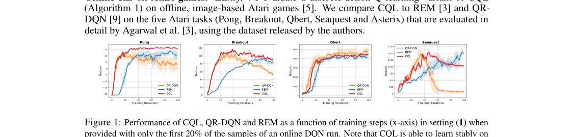
Figure 1: Performance of CQL, QR-DQN and REM as a function of training steps (x-axis) in setting (1) when provided with only the first 20% of the samples of an online DQN run. Note that CQL is able to learn stably on 3 out of 4 games, and its performance does not degrade as steeply as QR-DQN on Seaquest∗.
图 1:设定 (1) 下,仅提供在线 DQN 运行前 20% 样本时,CQL、QR-DQN 与 REM 随训练步数(横轴)的表现。注意 CQL 在 4 款游戏中的 3 款上能稳定学习,且在 Seaquest∗ 上表现下降不如 QR-DQN 陡峭。
Following the evaluation protocol of Agarwal et al. 2019, we evaluated on two types of datasets, both of which were generated from the DQN-replay dataset, released by [3]: (1) a dataset consisting of the first 20% of the samples observed by an online DQN agent and (2) datasets consisting of only 1% and 10% of all samples observed by an online DQN agent (Figures 6 and 7 in [3]). In setting (1), shown in Figure 1, CQL generally achieves similar or better performance throughout as QR-DQN and REM. When only using only 1% or 10% of the data, in setting (2) (Table 3), CQL
沿用 Agarwal 等 2019 的评估协议,我们在两类均由 [3] 发布的 DQN-replay 数据集生成的数据上评估:(1) 在线 DQN 智能体观测到的前 20% 样本;(2) 仅含该智能体全部观测样本的 1% 与 10%(见 [3] 图 6、7)。在设定 (1)(图 1)中,CQL 全程表现通常与 QR-DQN、REM 相当或更好。在设定 (2) 仅用 1% 或 10% 数据时(表 3),CQL
| Task Name | QR-DQN | REM | CQL() |
|---|---|---|---|
| Pong (1%) | -13.8 | -6.9 | 19.3 |
| Breakout | 7.9 | 11.0 | 61.1 |
| Q*bert | 383.6 | 343.4 | 14012.0 |
| Seaquest | 672.9 | 499.8 | 779.4 |
| Asterix | 166.3 | 386.5 | 592.4 |
| Pong (10%) | 15.1 | 8.9 | 18.5 |
| Breakout | 151.2 | 86.7 | 269.3 |
| Q*bert | 7091.3 | 8624.3 | 13855.6 |
| Seaquest | 2984.8 | 3936.6 | 3674.1 |
| Asterix | 189.2 | 75.1 | 156.3 |
Table 3: CQL, REM and QR-DQN in setting (1) with 1% data (top), and 10% data (bottom). CQL drastically outperforms prior methods with 1% data, and usually attains better performance with 10% data.
| 任务名 | QR-DQN | REM | CQL() |
|---|---|---|---|
| Pong (1%) | -13.8 | -6.9 | 19.3 |
| Breakout | 7.9 | 11.0 | 61.1 |
| Q*bert | 383.6 | 343.4 | 14012.0 |
| Seaquest | 672.9 | 499.8 | 779.4 |
| Asterix | 166.3 | 386.5 | 592.4 |
| Pong (10%) | 15.1 | 8.9 | 18.5 |
| Breakout | 151.2 | 86.7 | 269.3 |
| Q*bert | 7091.3 | 8624.3 | 13855.6 |
| Seaquest | 2984.8 | 3936.6 | 3674.1 |
| Asterix | 189.2 | 75.1 | 156.3 |
表 3:设定 (1) 下 CQL、REM 与 QR-DQN 在 1% 数据(上)与 10% 数据(下)上的结果。1% 数据时 CQL 大幅领先先验方法;10% 数据时通常也更好。
substantially outperforms REM and QR-DQN, especially in the harder 1% condition, achieving 36x and 6x times the return of the best prior method on Q*bert and Breakout, respectively.
大幅优于 REM 与 QR-DQN,尤其在更难的 1% 条件下:在 Q*bert 与 Breakout 上分别达到最优先验方法回报的 36 倍与 6 倍。
Analysis of CQL. Finally, we perform empirical evaluation to verify that CQL indeed lower-bounds the value function, thus verifying Theorems 3.2, Appendix D.1 empirically. To this end, we estimate the average value of the learned policy predicted by CQL, , and report the difference against the actual discounted return of the policy in Table 4. We also estimate these values for baselines, including the minimum predicted Q-value under an ensemble [21, 18] of Q-functions with varying ensemble sizes, which is a standard technique to prevent overestimed Q-values [18, 21, 23] and BEAR [32], a policy constraint method. The results show that CQL learns a lower bound for all three tasks, whereas the baselines are prone to overestimation. We also evaluate a variant of CQL that uses Equation 1, and observe that the resulting values are lower (that is, underestimate the true values) as compared to CQL(). This provides empirical evidence that CQL() attains a tighter lower bound than the point-wise bound in Equation 1, as per Theorem 3.2.
CQL 分析。 最后做经验评估,验证 CQL 确实下界价值函数,从而经验地验证定理 3.2 与附录 D.1。为此,估计 CQL 预测的所学策略平均价值 ,并在表 4 中报告其与策略 真实折扣回报之差。我们也对基线估计这些值,包括不同规模集成下取最小预测 Q 值 [21, 18](防止 Q 高估的标准技术 [18, 21, 23])以及策略约束方法 BEAR [32]。结果显示 CQL 在全部三项任务上学到下界,而基线易高估。我们还评估使用式 1 的 CQL 变体,观察到所得值低于 CQL()(即更低估真实值)。这为定理 3.2 提供经验证据:CQL() 比式 1 的点态下界更紧。
| Task Name | CQL( | CQL (Eqn. 1) | Ensemble(2) | Ens.(4) | Ens.(10) | Ens.(20) | BEAR |
|---|---|---|---|---|---|---|---|
| hopper-medium-expert | -43.20 | -151.36 | 3.71e6 | 2.93e6 | 0.32e6 | 24.05e3 | 65.93 |
| hopper-mixed | -10.93 | -22.87 | 15.00e6 | 59.93e3 | 8.92e3 | 2.47e3 | 1399.46 |
| hopper-medium | -7.48 | -156.70 | 26.03e12 | 437.57e6 | 1.12e12 | 885e3 | 4.32 |
Table 4: Difference between policy values predicted by each algorithm and the true policy value for CQL, a variant of CQL that uses Equation 1, the minimum of an ensemble of varying sizes, and BEAR [32] on three D4RL datasets. CQL is the only method that lower-bounds the actual return (i.e., has negative differences), and CQL( is much less conservative than CQL (Eqn. 1).
| 任务名 | CQL( | CQL (式 1) | Ensemble(2) | Ens.(4) | Ens.(10) | Ens.(20) | BEAR |
|---|---|---|---|---|---|---|---|
| hopper-medium-expert | -43.20 | -151.36 | 3.71e6 | 2.93e6 | 0.32e6 | 24.05e3 | 65.93 |
| hopper-mixed | -10.93 | -22.87 | 15.00e6 | 59.93e3 | 8.92e3 | 2.47e3 | 1399.46 |
| hopper-medium | -7.48 | -156.70 | 26.03e12 | 437.57e6 | 1.12e12 | 885e3 | 4.32 |
表 4:各算法预测的策略价值与真实策略价值之差,涵盖 CQL、使用式 1 的 CQL 变体、不同规模集成的最小值,以及 BEAR [32],数据为三个 D4RL 数据集。CQL 是唯一下界真实回报的方法(差值为负),且 CQL( 远不如 CQL(式 1)保守。
We also present an empirical analysis to show that Theorem 3.4, that CQL is gap-expanding, holds in practice in Appendix B, and present an ablation study on various design choices used in CQL in Appendix G.
我们还在附录 B 给出经验分析,说明定理 3.4(CQL 具有间隙扩张性)在实践中成立,并在附录 G 对 CQL 的各项设计选择做消融。
7 Discussion
7 讨论
We proposed conservative Q-learning (CQL), an algorithmic framework for offline RL that learns a lower bound on the policy value. Empirically, we demonstrate that CQL outperforms prior offline RL methods on a wide range of offline RL benchmark tasks, including complex control tasks and tasks with raw image observations. In many cases, the performance of CQL is substantially better than the best-performing prior methods, exceeding their final returns by 2-5x. The simplicity and efficacy of CQL make it a promising choice for a wide range of real-world offline RL problems. However, a number of challenges remain. While we prove that CQL learns lower bounds on the Q-function in the tabular, linear, and a subset of non-linear function approximation cases, a rigorous theoretical analysis of CQL with deep neural nets, is left for future work. Additionally, offline RL methods are liable to suffer from overfitting in the same way as standard supervised methods, so another important challenge for future work is to devise simple and effective early stopping methods, analogous to validation error in supervised learning.
我们提出保守 Q 学习(CQL)这一离线 RL 算法框架,学习策略价值的下界。经验上,CQL 在广泛的离线 RL 基准上优于先验方法,包括复杂控制任务与原始图像观测任务。许多情形下 CQL 表现远超最优先验方法,最终回报可达其 2–5 倍。CQL 的简洁与有效使其成为广泛真实世界离线 RL 问题的有希望选择。但仍有若干挑战:我们证明了 CQL 在表格、线性以及部分非线性函数逼近情形下学习 Q 函数下界,但对深度神经网络的严格理论分析留待未来工作。此外,离线 RL 方法与标准监督方法一样可能过拟合,另一重要未来方向是设计类似监督学习验证误差的简单有效早停方法。
Acknowledgements
致谢
We thank Mohammad Norouzi, Oleh Rybkin, Anton Raichuk, Vitchyr Pong and anonymous reviewers from the Robotic AI and Learning Lab at UC Berkeley for their feedback on an earlier version of this paper. We thank Rishabh Agarwal for help with the Atari QR-DQN/REM codebase and for sharing baseline results. This research was funded by the DARPA Assured Autonomy program, and compute support from Google, Amazon, and NVIDIA.
感谢 Mohammad Norouzi、Oleh Rybkin、Anton Raichuk、Vitchyr Pong 以及 UC Berkeley Robotic AI and Learning Lab 匿名审稿人对本文早期版本的反馈。感谢 Rishabh Agarwal 在 Atari QR-DQN/REM 代码库上的帮助并分享基线结果。本研究由 DARPA Assured Autonomy 项目资助,并获 Google、Amazon 与 NVIDIA 的算力支持。
References
参考文献
Achiam et al. [2017] Joshua Achiam, David Held, Aviv Tamar, and Pieter Abbeel. Constrained policy optimization. In Proceedings of the 34th International Conference on Machine Learning-Volume 70 , pages 22–31. JMLR. org, 2017.
Achiam et al. [2019] Joshua Achiam, Ethan Knight, and Pieter Abbeel. Towards characterizing divergence in deep q-learning. arXiv preprint arXiv:1903.08894 , 2019.
Agarwal et al. [2019] Rishabh Agarwal, Dale Schuurmans, and Mohammad Norouzi. An optimistic perspective on offline reinforcement learning. 2019.
[4] DeepMind AlphaStar. Mastering the real-time strategy game starcraft ii. URL: https://deepmind. com/blog/alphastar-mastering-real-time-strategy-game-starcraft-ii .
Bellemare et al. [2013] Marc G Bellemare, Yavar Naddaf, Joel Veness, and Michael Bowling. The arcade learning environment: An evaluation platform for general agents. Journal of Artificial Intelligence Research , 47:253–279, 2013.
Bellemare et al. [2016] Marc G Bellemare, Georg Ostrovski, Arthur Guez, Philip S Thomas, and Rémi Munos. Increasing the action gap: New operators for reinforcement learning. In Thirtieth AAAI Conference on Artificial Intelligence , 2016.
Burda et al. [2018] Yuri Burda, Harrison Edwards, Amos Storkey, and Oleg Klimov. Exploration by random network distillation. arXiv preprint arXiv:1810.12894 , 2018.
Chen and Jiang [2019] Jinglin Chen and Nan Jiang. Information-theoretic considerations in batch reinforcement learning. arXiv preprint arXiv:1905.00360 , 2019.
Dabney et al. [2018] Will Dabney, Mark Rowland, Marc G Bellemare, and Rémi Munos. Distributional reinforcement learning with quantile regression. In Thirty-Second AAAI Conference on Artificial Intelligence , 2018.
Deng et al. [2009] Jia Deng, Wei Dong, Richard Socher, Li-Jia Li, Kai Li, and Li Fei-Fei. Imagenet: A large-scale hierarchical image database. In 2009 IEEE conference on computer vision and pattern recognition , pages 248–255. Ieee, 2009.
Devlin et al. [2018] Jacob Devlin, Ming-Wei Chang, Kenton Lee, and Kristina Toutanova. Bert: Pre-training of deep bidirectional transformers for language understanding. arXiv preprint arXiv:1810.04805 , 2018.
Ernst et al. [2005] Damien Ernst, Pierre Geurts, and Louis Wehenkel. Tree-based batch mode reinforcement learning. Journal of Machine Learning Research , 6(Apr):503–556, 2005.
Farahmand et al. [2010] Amir-massoud Farahmand, Csaba Szepesvári, and Rémi Munos. Error propagation for approximate policy and value iteration. In Advances in Neural Information Processing Systems , pages 568–576, 2010.
Fu et al. [2020a] J. Fu, A. Kumar, O. Nachum, G. Tucker, and S. Levine. D4rl: Datasets for deep data-driven reinforcement learning. In arXiv , 2020a. URL https://arxiv.org/pdf/2004.07219 .
Fu et al. [2019] Justin Fu, Aviral Kumar, Matthew Soh, and Sergey Levine. Diagnosing bottlenecks in deep Q-learning algorithms. arXiv preprint arXiv:1902.10250 , 2019.
Fu et al. [2020b] Justin Fu, Aviral Kumar, Ofir Nachum, George Tucker, and Sergey Levine. D4rl: Datasets for data-driven deep reinforcement learning. https://github.com/rail-berkeley/d4rl/wiki/New-Franka-Kitchen-Tasks , 2020b. Github repository.
Fujimoto et al. [2018a] Scott Fujimoto, David Meger, and Doina Precup. Off-policy deep reinforcement learning without exploration. arXiv preprint arXiv:1812.02900 , 2018a.
Fujimoto et al. [2018b] Scott Fujimoto, Herke van Hoof, and David Meger. Addressing function approximation error in actor-critic methods. In International Conference on Machine Learning (ICML) , pages 1587–1596, 2018b.
Gelada and Bellemare [2019] Carles Gelada and Marc G Bellemare. Off-policy deep reinforcement learning by bootstrapping the covariate shift. In Proceedings of the AAAI Conference on Artificial Intelligence , volume 33, pages 3647–3655, 2019.
Gupta et al. [2019] Abhishek Gupta, Vikash Kumar, Corey Lynch, Sergey Levine, and Karol Hausman. Relay policy learning: Solving long-horizon tasks via imitation and reinforcement learning. arXiv preprint arXiv:1910.11956 , 2019.
Haarnoja et al. [2017] T. Haarnoja, H. Tang, P. Abbeel, and S. Levine. Reinforcement learning with deep energy-based policies. In International Conference on Machine Learning (ICML) , 2017.
Hallak and Mannor [2017] Assaf Hallak and Shie Mannor. Consistent on-line off-policy evaluation. In Proceedings of the 34th International Conference on Machine Learning-Volume 70 , pages 1372–1383. JMLR. org, 2017.
Hasselt [2010] Hado V Hasselt. Double q-learning. In Advances in neural information processing systems , pages 2613–2621, 2010.
He et al. [2016] Kaiming He, Xiangyu Zhang, Shaoqing Ren, and Jian Sun. Deep residual learning for image recognition. In Proceedings of the IEEE conference on computer vision and pattern recognition , pages 770–778, 2016.
Hester et al. [2018] Todd Hester, Matej Vecerik, Olivier Pietquin, Marc Lanctot, Tom Schaul, Bilal Piot, Dan Horgan, John Quan, Andrew Sendonaris, Ian Osband, et al. Deep q-learning from demonstrations. In Thirty-Second AAAI Conference on Artificial Intelligence , 2018.
Iyengar [2005] Garud N Iyengar. Robust dynamic programming. Mathematics of Operations Research , 30(2):257–280, 2005.
Jacot et al. [2018] Arthur Jacot, Franck Gabriel, and Clement Hongler. Neural tangent kernel: Convergence and generalization in neural networks. In Advances in Neural Information Processing Systems 31 . 2018.
Jaksch et al. [2010] Thomas Jaksch, Ronald Ortner, and Peter Auer. Near-optimal regret bounds for reinforcement learning. Journal of Machine Learning Research , 11(Apr):1563–1600, 2010.
Jaques et al. [2019] Natasha Jaques, Asma Ghandeharioun, Judy Hanwen Shen, Craig Ferguson, Agata Lapedriza, Noah Jones, Shixiang Gu, and Rosalind Picard. Way off-policy batch deep reinforcement learning of implicit human preferences in dialog. arXiv preprint arXiv:1907.00456 , 2019.
Kakade and Langford [2002] Sham Kakade and John Langford. Approximately optimal approximate reinforcement learning. In International Conference on Machine Learning (ICML) , volume 2, 2002.
Kalashnikov et al. [2018] Dmitry Kalashnikov, Alex Irpan, Peter Pastor, Julian Ibarz, Alexander Herzog, Eric Jang, Deirdre Quillen, Ethan Holly, Mrinal Kalakrishnan, Vincent Vanhoucke, et al. Scalable deep reinforcement learning for vision-based robotic manipulation. In Conference on Robot Learning , pages 651–673, 2018.
Kumar et al. [2019] Aviral Kumar, Justin Fu, Matthew Soh, George Tucker, and Sergey Levine. Stabilizing off-policy q-learning via bootstrapping error reduction. In Advances in Neural Information Processing Systems , pages 11761–11771, 2019.
Kumar et al. [2020] Aviral Kumar, Abhishek Gupta, and Sergey Levine. Discor: Corrective feedback in reinforcement learning via distribution correction. arXiv preprint arXiv:2003.07305 , 2020.
Lagoudakis and Parr [2003] Michail G Lagoudakis and Ronald Parr. Least-squares policy iteration. Journal of machine learning research , 4(Dec):1107–1149, 2003.
Laroche et al. [2017] Romain Laroche, Paul Trichelair, and Rémi Tachet des Combes. Safe policy improvement with baseline bootstrapping. arXiv preprint arXiv:1712.06924 , 2017.
Levine et al. [2020] Sergey Levine, Aviral Kumar, George Tucker, and Justin Fu. Offline reinforcement learning: Tutorial, review, and perspectives on open problems. arXiv preprint arXiv:2005.01643 , 2020.
Li et al. [2010] Lihong Li, Wei Chu, John Langford, and Robert E Schapire. A contextual-bandit approach to personalized news article recommendation. In Proceedings of the 19th international conference on World wide web , pages 661–670, 2010.
Liu et al. [2018] Qiang Liu, Lihong Li, Ziyang Tang, and Dengyong Zhou. Breaking the curse of horizon: Infinite-horizon off-policy estimation. In Advances in Neural Information Processing Systems , pages 5356–5366, 2018.
Lu et al. [2018] Yingdong Lu, Mark S Squillante, and Chai Wah Wu. A general family of robust stochastic operators for reinforcement learning. arXiv preprint arXiv:1805.08122 , 2018.
Luo et al. [2019] Yuping Luo, Huazhe Xu, and Tengyu Ma. Learning self-correctable policies and value functions from demonstrations with negative sampling. arXiv preprint arXiv:1907.05634 , 2019.
Mnih et al. [2013] Volodymyr Mnih, Koray Kavukcuoglu, David Silver, Alex Graves, Ioannis Antonoglou, Daan Wierstra, and Martin Riedmiller. Playing atari with deep reinforcement learning. arXiv preprint arXiv:1312.5602 , 2013.
Nachum et al. [2019] Ofir Nachum, Yinlam Chow, Bo Dai, and Lihong Li. Dualdice: Behavior-agnostic estimation of discounted stationary distribution corrections. In Advances in Neural Information Processing Systems , pages 2315–2325, 2019.
Nadjahi et al. [2019] Kimia Nadjahi, Romain Laroche, and Rémi Tachet des Combes. Safe policy improvement with soft baseline bootstrapping. arXiv preprint arXiv:1907.05079 , 2019.
Nair et al. [2020] Ashvin Nair, Murtaza Dalal, Abhishek Gupta, and Sergey Levine. Accelerating online reinforcement learning with offline datasets. arXiv preprint arXiv:2006.09359 , 2020.
Namkoong and Duchi [2017] Hongseok Namkoong and John C Duchi. Variance-based regularization with convex objectives. In Advances in neural information processing systems , pages 2971–2980, 2017.
Nilim and El Ghaoui [2004] Arnab Nilim and Laurent El Ghaoui. Robustness in markov decision problems with uncertain transition matrices. In Advances in neural information processing systems , pages 839–846, 2004.
O’Donoghue [2018] Brendan O’Donoghue. Variational bayesian reinforcement learning with regret bounds. arXiv preprint arXiv:1807.09647 , 2018.
Osband and Van Roy [2017] Ian Osband and Benjamin Van Roy. Why is posterior sampling better than optimism for reinforcement learning? In Proceedings of the 34th International Conference on Machine Learning-Volume 70 , pages 2701–2710. JMLR. org, 2017.
Osband et al. [2016] Ian Osband, Charles Blundell, Alexander Pritzel, and Benjamin Van Roy. Deep exploration via bootstrapped dqn. In Advances in neural information processing systems , pages 4026–4034, 2016.
Peng et al. [2019] Xue Bin Peng, Aviral Kumar, Grace Zhang, and Sergey Levine. Advantage-weighted regression: Simple and scalable off-policy reinforcement learning. arXiv preprint arXiv:1910.00177 , 2019.
Peshkin and Shelton [2002] Leonid Peshkin and Christian R Shelton. Learning from scarce experience. arXiv preprint cs/0204043 , 2002.
Petrik et al. [2016] Marek Petrik, Mohammad Ghavamzadeh, and Yinlam Chow. Safe policy improvement by minimizing robust baseline regret. In Advances in Neural Information Processing Systems , pages 2298–2306, 2016.
Precup [2000] Doina Precup. Eligibility traces for off-policy policy evaluation. Computer Science Department Faculty Publication Series , page 80, 2000.
Precup et al. [2001] Doina Precup, Richard S Sutton, and Sanjoy Dasgupta. Off-policy temporal-difference learning with function approximation. In ICML , pages 417–424, 2001.
Rajeswaran et al. [2018] Aravind Rajeswaran, Vikash Kumar, Abhishek Gupta, Giulia Vezzani, John Schulman, Emanuel Todorov, and Sergey Levine. Learning complex dexterous manipulation with deep reinforcement learning and demonstrations. In Robotics: Science and Systems , 2018.
Scherrer [2014] Bruno Scherrer. Approximate policy iteration schemes: a comparison. In International Conference on Machine Learning , pages 1314–1322, 2014.
Siegel et al. [2020] Noah Y Siegel, Jost Tobias Springenberg, Felix Berkenkamp, Abbas Abdolmaleki, Michael Neunert, Thomas Lampe, Roland Hafner, and Martin Riedmiller. Keep doing what worked: Behavioral modelling priors for offline reinforcement learning. arXiv preprint arXiv:2002.08396 , 2020.
Simão et al. [2019] Thiago D Simão, Romain Laroche, and Rémi Tachet des Combes. Safe policy improvement with an estimated baseline policy. arXiv preprint arXiv:1909.05236 , 2019.
Tamar et al. [2014] Aviv Tamar, Shie Mannor, and Huan Xu. Scaling up robust mdps using function approximation. In International Conference on Machine Learning , pages 181–189, 2014.
Thomas et al. [2015] Philip Thomas, Georgios Theocharous, and Mohammad Ghavamzadeh. High confidence policy improvement. In International Conference on Machine Learning , pages 2380–2388, 2015.
Vecerik et al. [2017] Mel Vecerik, Todd Hester, Jonathan Scholz, Fumin Wang, Olivier Pietquin, Bilal Piot, Nicolas Heess, Thomas Rothörl, Thomas Lampe, and Martin Riedmiller. Leveraging demonstrations for deep reinforcement learning on robotics problems with sparse rewards. arXiv preprint arXiv:1707.08817 , 2017.
Wu et al. [2019] Yifan Wu, George Tucker, and Ofir Nachum. Behavior regularized offline reinforcement learning. arXiv preprint arXiv:1911.11361 , 2019.
Xie and Jiang [2020] Tengyang Xie and Nan Jiang. Q* approximation schemes for batch reinforcement learning: A eoretical comparison. 2020.
Zhang et al. [2020] Ruiyi Zhang, Bo Dai, Lihong Li, and Dale Schuurmans. Gendice: Generalized offline estimation of stationary values. In International Conference on Learning Representations , 2020. URL https://openreview.net/forum?id=HkxlcnVFwB .
Appendices
附录
Appendix A Discussion of CQL Variants
附录 A CQL 变体讨论
We derive several variants of CQL in Section 3.2. Here, we discuss these variants on more detail and describe their specific properties. We first derive the variants: CQL(), CQL(), and then present another variant of CQL, which we call CQL(var). This third variant has strong connections to distributionally robust optimization [45].
我们在第 3.2 节导出了若干 CQL 变体。这里更详细讨论这些变体并描述其具体性质。先导出 CQL()、CQL(),再给出另一变体 CQL(var);第三种变体与分布鲁棒优化 [45] 有很强联系。
CQL(). In order to derive CQL(), we substitute , and solve the optimization over in closed form for a given Q-function. For an optimization problem of the form:
CQL()。 为导出 CQL(),令 ,并对给定 Q 函数闭式求解对 的优化。对如下形式的优化问题:
the optimal solution is equal to , where is a normalizing factor. Plugging this into Equation 3, we exactly obtain Equation 4.
最优解为 ,其中 为归一化因子。代入式 3,恰好得到式 4。
CQL(). In order to derive CQL(), we follow the above derivation, but our regularizer is a KL-divergence regularizer instead of entropy.
CQL()。 为导出 CQL(),沿用上述推导,但正则子改为 KL 散度而非熵。
The optimal solution is given by, , where is a normalizing factor. Plugging this back into the CQL family (Equation 3), we obtain the following objective for training the Q-function (modulo some normalization terms):
最优解为 ,其中 为归一化因子。代回 CQL 族(式 3),得到训练 Q 函数的如下目标(略去若干归一化项):
CQL(var). Finally, we derive a CQL variant that is inspired from the perspective of distributionally robust optimization (DRO) [45]. This version penalizes the variance in the Q-function across actions at all states , under some action-conditional distribution of our choice. In order to derive a canonical form of this variant, we invoke an identity from Namkoong and Duchi 2017, which helps us simplify Equation 3. To start, we define the notion of “robust expectation”: for any function , and any empirical distribution over a dataset of elements, the “robust” expectation defined by:
CQL(var)。 最后从分布鲁棒优化(DRO) [45] 视角导出一个 CQL 变体。该版本在我们选择的动作条件分布下,惩罚所有状态 上跨动作的 Q 函数方差。为得到规范形式,我们援引 Namkoong 与 Duchi 2017 的恒等式以简化式 3。首先定义「鲁棒期望」:对任意函数 ,以及对 元数据集 上的任意经验分布 ,「鲁棒」期望定义为:
can be approximated using the following upper-bound:
可用如下上界近似:
where the gap between the two sides of the inequality decays inversely w.r.t. to the dataset size, . By using Equation 8 to simplify Equation 3, we obtain an objective for training the Q-function that penalizes the variance of Q-function predictions under the distribution .
其中不等式两边间隙随数据集规模按 衰减。用式 8 简化式 3,得到在分布 下惩罚 Q 函数预测方差的训练目标。
$$\min_{Q}~~\frac{1}{2}~\mathbb{E}{\mathbf{s},\mathbf{a},\mathbf{s}^{\prime}\sim\mathcal{D}}\left[\left(Q-\mathcal{B}^{\pi{k}}\hat{Q}^{k}\right)^{2}\right]+\alpha\mathbb{E}{\mathbf{s}\sim d^{\pi{\beta}}(\mathbf{s})}\left[\sqrt{\frac{\text{var}{\hat{P}(\mathbf{a}|\mathbf{s})}\left(Q(\mathbf{s},\mathbf{a})\right)}{d^{\pi{\beta}}(s)|\mathcal{D}|}}\right]\
+\alpha\mathbb{E}{s\sim d^{\pi{\beta}}(\mathbf{s})}\left[\mathbb{E}{\hat{P}(\mathbf{a}|\mathbf{s})}[Q(\mathbf{s},\mathbf{a})]-\mathbb{E}{{\pi_{\beta}}(\mathbf{a}|\mathbf{s})}[Q(\mathbf{s},\mathbf{a})]\right] \tag{9}$$
The only remaining decision is the choice of , which can be chosen to be the inverse of the empirical action distribution in the dataset, , or even uniform over actions, , to obtain this variant of variance-regularized CQL.
剩下只需选择 :可取数据集中经验动作分布的倒数 ,或对动作均匀 ,从而得到该方差正则化 CQL 变体。
Appendix B Discussion of Gap-Expanding Behavior of CQL Backups
附录 B CQL 回传间隙扩张行为的讨论
In this section, we discuss in detail the consequences of the gap-expanding behavior of CQL backups over prior methods based on policy constraints that, as we show in this section, may not exhibit such gap-expanding behavior in practice. To recap, Theorem 3.4 shows that the CQL backup operator increases the difference between expected Q-value at in-distribution () and out-of-distribution () actions. We refer to this property as the gap-expanding property of the CQL update operator.
本节详细讨论 CQL 回传的间隙扩张行为相对基于策略约束的先验方法的后果;我们将表明后者实践中未必呈现此类间隙扩张。回顾定理 3.4:CQL 回传算子增大分布内动作()与分布外动作()上期望 Q 值之差。我们称 CQL 更新算子的这一性质为间隙扩张性质。
Function approximation may give rise to erroneous Q-values at OOD actions. We start by discussing the behavior of prior methods based on policy constraints [32, 17, 29, 62] in the presence of function approximation. To recap, because computing the target value requires , constraining to be close to will avoid evaluating on OOD actions. These methods typically do not impose any further form of regularization on the learned Q-function. Even with policy constraints, because function approximation used to represent the Q-function, learned Q-values at two distinct state-action pairs are coupled together. As prior work has argued and shown [2, 15, 33], the “generalization” or the coupling effects of the function approximator may be heavily influenced by the properties of the data distribution [15, 33]. For instance, Fu et al. 2019 empirically shows that when the dataset distribution is narrow (i.e. state-action marginal entropy, , is low [15]), the coupling effects of the Q-function approximator can give rise to incorrect Q-values at different states, though this behavior is absent without function approximation, and is not as severe with high-entropy (e.g. Uniform) state-action marginal distributions.
函数逼近可能在 OOD 动作上产生错误 Q 值。 我们先讨论基于策略约束的先验方法 [32, 17, 29, 62] 在函数逼近下的行为。回顾:计算目标值需要 ,约束 靠近 可避免在 OOD 动作上评估 。这些方法通常不对所学 Q 函数施加进一步正则。即便有策略约束,由于用函数逼近表示 Q,不同状态—动作对上学到的 Q 值彼此耦合。如先验工作所论证与展示 [2, 15, 33],函数逼近器的「泛化」或耦合效应可能强烈受数据分布性质影响 [15, 33]。例如 Fu 等 2019 经验表明:当数据集分布较窄(即状态—动作边际熵 低 [15])时,Q 函数逼近器的耦合可能在不同状态上给出不正确的 Q 值;无函数逼近时该现象不存在,且在高熵(如均匀)状态—动作边际分布下也不那么严重。
In offline RL, we will shortly present empirical evidence on high-dimensional MuJoCo tasks showing that certain dataset distributions, , may cause the learned Q-value at an OOD action at a state , to in fact take on high values than Q-values at in-distribution actions at intermediate iterations of learning. This problem persists even when a large number of samples (e.g. ) are provided for training, and the agent cannot correct these errors due to no active data collection.
在离线 RL 中,我们稍后在高维 MuJoCo 任务上给出经验证据:某些数据集分布 可能使某状态 上 OOD 动作 的所学 Q 值,在学习中期迭代中反而高于分布内动作的 Q 值。即便提供大量样本(如 )用于训练,由于无法主动采集数据,智能体仍无法纠正这些误差。
Since actor-critic methods, including those with policy constraints, use the learned Q-function to train the policy, in an iterative online policy evaluation and policy improvement cycle, as discussed in Section 2, the errneous Q-function may push the policy towards OOD actions, especially when no policy constraints are used. Of course, policy constraints should prevent the policy from choosing OOD actions, however, as we will show that in certain cases, policy constraint methods might also fail to prevent the effects on the policy due to incorrectly high Q-values at OOD actions.
由于 actor-critic 方法(含带策略约束者)用所学 Q 训练策略,并在第 2 节所述的迭代在线策略评估与改进循环中运行,错误的 Q 函数可能把策略推向 OOD 动作,尤其在不使用策略约束时。当然,策略约束本应阻止策略选择 OOD 动作;但我们将表明,在某些情形下,策略约束方法也可能无法阻止 OOD 动作上错误偏高 Q 值对策略的影响。
How can CQL address this problem? As we show in Theorem 3.4, the difference between expected Q-values at in-distribution actions and out-of-distribution actions is expanded by the CQL update. This property is a direct consequence of the specific nature of the CQL regularizer – that maximizes Q-values under the dataset distribution, and minimizes them otherwise. This difference depends upon the choice of , which can directly be controlled, since it is a free parameter. Thus, by effectively controlling , CQL can push down the learned Q-value at out-of-distribution actions as much is desired, correcting for the erroneous overestimation error in the process.
CQL 如何应对? 如定理 3.4 所示,CQL 更新会扩大分布内与分布外动作上期望 Q 值之差。该性质直接来自 CQL 正则子的具体形式——在数据分布下最大化 Q 值、在其他处最小化。该差依赖于可自由控制的 。因此,通过有效控制 ,CQL 可按需压低分布外动作上的所学 Q 值,从而纠正错误高估。
Empirical evidence on high-dimensional benchmarks with neural networks. We next empirically demonstrate the existence of of such Q-function estimation error on high-dimensional MuJoCo domains when deep neural network function approximators are used with stochastic optimization techniques. In order to measure this error, we plot the difference in expected Q-value under actions sampled from the behavior distribution, , and the maximum Q-value over actions sampled from a uniformly random policy, . That is, we plot the quantity
高维基准上使用神经网络的经验证据。 接下来经验展示:在高维 MuJoCo 领域、以深度神经网络函数逼近器配合随机优化时,确存在此类 Q 函数估计误差。为度量该误差,我们绘制行为分布采样动作 上的期望 Q 值,与均匀随机策略采样动作 上最大 Q 值之差。即绘制量
over the iterations of training, indexed by . This quantity, intuitively, represents an estimate of the “advantage” of an action , under the Q-function, with respect to the optimal action . Since, we cannot perform exact maximization over the learned Q-function in a continuous action space to compute , we estimate it via sampling described in Equation 10.
随训练迭代 的变化。该量直观上估计动作 在 Q 函数下相对最优动作 的「优势」。由于连续动作空间中无法对所学 Q 做精确最大化以计算 ,我们用式 10 所述采样来估计。
We present these plots in Figure 2 on two datasets: hopper-expert and hopper-medium. The expert dataset is generated from a near-deterministic, expert policy, exhibits a narrow coverage of the state-action space, and limited to only a few directed trajectories. On this dataset, we find that is always positive for the policy constraint method (Figure 2(a)) and increases during training – note, the continuous rise in values, in the case of the policy-constraint method, shown in Figure 2(a). This means that even if the dataset is generated from an expert policy, and policy constraints correct target values for OOD actions, incorrect Q-function generalization may make an out-of-distribution action appear promising. For the more stochastic hopper-medium dataset, that consists of a more diverse set of trajectories, shown in Figure 2(b), we still observe that for the policy-constraint method, however, the relative magnitude is smaller than hopper-expert.
我们在图 2 中给出 hopper-expert 与 hopper-medium 两个数据集上的曲线。专家数据集由近确定性专家策略生成,状态—动作空间覆盖窄,且仅含少量有向轨迹。在该数据集上,策略约束方法的 始终为正(图 2(a))并在训练中上升——注意图 2(a) 中策略约束方法 的持续攀升。这意味着即便数据来自专家策略、且策略约束已纠正 OOD 动作的目标值,错误的 Q 泛化仍可能使分布外动作看起来有希望。对由更多样轨迹组成、更随机的 hopper-medium 数据集(图 2(b)),策略约束方法仍有 ,但相对幅度小于 hopper-expert。
In contrast, Q-functions learned by CQL, generally satisfy , as is seen and these values are clearly smaller than those for the policy-constraint method. This provides some empirical evidence for Theorem 3.4, in that, the maximum Q-value at a randomly chosen action from the uniform distribution the action space is smaller than the Q-value at in-distribution actions.
相比之下,CQL 学到的 Q 函数通常满足 ,且明显小于策略约束方法。这为定理 3.4 提供了若干经验证据:在动作空间均匀分布上随机选取动作的最大 Q 值,小于分布内动作的 Q 值。
On the hopper-expert task, as we show in Figure 2(a) (right), we eventually observe an “unlearning” effect, in the policy-constraint method where the policy performance deteriorates after a extra iterations in training. This “unlearning” effect is similar to what has been observed when standard off-policy Q-learning algorithms without any policy constraint are used in the offline regime [32, 36], on the other hand this effect is absent in the case of CQL, even after equally many training steps. The performance in the more-stochastic hopper-medium dataset fluctuates, but does not deteriorate suddenly.
在 hopper-expert 任务上,如图 2(a)(右)所示,策略约束方法最终出现「反学习(unlearning)」:再训练若干迭代后策略表现恶化。该效应类似于在离线设定中使用无策略约束的标准异策略 Q 学习时所见 [32, 36];而 CQL 即便训练步数同样多也不出现该效应。在更随机的 hopper-medium 数据集上,表现有波动,但不会突然恶化。
To summarize this discussion, we concretely observed the following points via empirical evidence:
小结本节讨论,经验证据具体表明:
- • CQL backups are gap expanding in practice, as justified by the negative values in Figure 2.
- • CQL 回传在实践中具有间隙扩张性,由图 2 中负的 值所印证。
- • Policy constraint methods, that do not impose any regularization on the Q-function may observe highly positive values during training, especially with narrow data distributions, indicating that gap-expansion may be absent.
- • 不对 Q 函数施加任何正则的策略约束方法,训练中可能观测到高度正的 ,尤其在窄数据分布上,表明间隙扩张可能缺失。
- • When values continuously grow during training, the policy might eventually suffer from an unlearning effect [36], as shown in Figure 2(a).
- • 当 在训练中持续增长时,策略最终可能遭受反学习效应 [36],如图 2(a) 所示。
(a) hopper-expert-v0
Appendix C Theorem Proofs
附录 C 定理证明
In this section, we provide proofs of the theorems in Sections 3.1 and 3.2. We first redefine notation for clarity and then provide the proofs of the results in the main paper.
本节给出第 3.1 与 3.2 节中定理的证明。先重定义记号以便清晰,再给出正文结果的证明。
Notation. Let denote an iteration of policy evaluation (in Section 3.1) or Q-iteration (in Section 3.2). In an iteration , the objective – Equation 2 or Equation 3 – is optimized using the previous iterate (i.e. ) as the target value in the backup. denotes the true, tabular Q-function iterate in the MDP, without any correction. In an iteration, say , the current tabular Q-function iterate, is related to the previous tabular Q-function iterate as: (for policy evaluation) or (for policy learning). Let denote the -th Q-function iterate obtained from CQL. Let denote the value function, .
记号。 令 表示策略评估(第 3.1 节)或 Q 迭代(第 3.2 节)的一次迭代。在迭代 ,目标——式 2 或式 3——以先前迭代(即 )作为回传中的目标值来优化。 表示 MDP 中无任何修正的真实表格 Q 函数迭代。在迭代 ,当前表格 Q 迭代 与上一表格迭代 的关系为:(策略评估)或 (策略学习)。令 表示由 CQL 得到的第 个 Q 函数迭代。令 表示价值函数 。
A note on the value of . Before proving the theorems, we remark that while the statements of Theorems 3.2, 3.1 and D.1 (we discuss this in Appendix D) show that CQL produces lower bounds if is larger than some threshold, so as to overcome either sampling error (Theorems 3.2 and 3.1) or function approximation error (Theorem D.1). While the optimal in some of these cases depends on the current Q-value, , we can always choose a worst-case value of by using the inequality , still guaranteeing a lower bound. If it is unclear why the learned Q-function should be bounded, we can always clamp the Q-values if they go outside .
关于 取值的说明。 在证明定理之前,我们指出:定理 3.2、3.1 与 D.1(见附录 D)的陈述表明,当 大于某一阈值以克服采样误差(定理 3.2、3.1)或函数逼近误差(定理 D.1)时,CQL 产生下界。尽管其中某些情形的最优 依赖于当前 Q 值 ,我们总能用不等式 选取最坏情形的 ,仍保证下界。若不清楚为何所学 应有界,可在 Q 值越出 时将其截断。
We first prove Theorem 3.1, which shows that policy evaluation using a simplified version of CQL (Equation 1) results in a point-wise lower-bound on the Q-function.
我们先证明定理 3.1:用简化版 CQL(式 1)做策略评估时,得到对 Q 函数的点态下界。
Proof of Theorem 3.1. In order to start, we first note that the form of the resulting Q-function iterate, , in the setting without function approximation. By setting the derivative of Equation 1 to 0, we obtain the following expression for in terms of ,
定理 3.1 的证明。 首先给出无函数逼近设定下所得 Q 迭代 的形式。令式 1 的导数为 0,得到 用 表示的表达式:
Now, since, , we observe that at each iteration we underestimate the next Q-value iterate, i.e. .
由于 ,可见每次迭代都低估下一 Q 值迭代,即 。
Accounting for sampling error. Note that so far we have only shown that the Q-values are upper-bounded by the the “empirical Bellman targets” given by, . In order to relate to the true Q-value iterate, , we need to relate the empirical Bellman operator, to the actual Bellman operator, . In Appendix D.3, we show that if the reward function and the transition function, satisfy “concentration” properties, meaning that the difference between the observed reward sample, () and the actual reward function (and analogously for the transition matrix) is bounded with high probability, then overestimation due to the empirical Backup operator is bounded. Formally, with high probability (w.h.p.) , ,
计入采样误差。 至此我们只证明了 Q 值被「经验 Bellman 目标」 上界。要把 与真实 Q 迭代 联系起来,还需把经验 Bellman 算子 与真实算子 联系起来。附录 D.3 表明:若奖励 与转移 满足「集中」性质——即观测奖励样本 ()与真实奖励 (转移矩阵类似)之差以高概率有界——则经验回传算子导致的高估有界。形式上,以高概率(w.h.p.),,
Hence, the following can be obtained, w.h.p.:
因此,以高概率可得:
Now we need to reason about the fixed point of the update procedure in Equation 11. The fixed point of Equation 11 is given by:
接下来需分析式 11 更新过程的不动点。式 11 的不动点为:
$$\hat{Q}^{\pi}\leq\mathcal{B}^{\pi}\hat{Q}^{\pi}-\alpha\frac{\mu(\mathbf{a}|\mathbf{s})}{\hat{\pi}{\beta}(\mathbf{a}|\mathbf{s})}+\frac{C{r,T,\delta}R_{\max}}{(1-\gamma)\sqrt{|\mathcal{D}(\mathbf{s},\mathbf{a})|}}\implies\hat{Q}^{\pi}\leq(I-\gamma P^{\pi})^{-1}\left[R-\alpha\frac{\mu}{\hat{\pi}{\beta}}+\frac{C{r,T,\delta}R_{\max}}{1-\gamma)\sqrt{|\mathcal{D}}}\right]\
\hat{Q}^{\pi}(\mathbf{s},\mathbf{a})\leq Q^{\pi}(\mathbf{s},\mathbf{a})-\alpha\left\left(I-\gamma P^{\pi}\right)^{-1}\left[\frac{\mu}{\hat{\pi}_{\beta}}\right]\right+\left(I-\gamma P^{\pi})^{-1}\frac{C_{r,T,\delta}R_{\max}}{(1-\gamma)\sqrt{|\mathcal{D}|}}\right,$$
thus proving the relationship in Theorem 3.1.
从而证明了定理 3.1 中的关系。
In order to guarantee a lower bound, can be chosen to cancel any potential overestimation incurred by . Note that this choice works, since is a matrix with all non-negative entries. The choice of that guarantees a lower bound is then given by:
为保证下界,可选取 以抵消 可能带来的任何高估。该选取可行,因为 是非负元矩阵。保证下界的 选取为:
Note that the theoretically minimum possible value of decreases as more samples are observed, i.e., when is large. Also, note that since, , when , any guarantees a lower bound. And so choosing a value of is sufficient in this case.
注意:随着观测样本增多,即 变大,理论最小可用 减小。还注意到:当 时 ,任意 都保证下界,因而此时取 即可。
Next, we prove Theorem 3.3 that shows that the additional term that maximizes the expected Q-value under the dataset distribution, , (or , in the absence of sampling error), results in a lower-bound on only the expected value of the policy at a state, and not a pointwise lower-bound on Q-values at all actions.
接下来证明定理 3.3:在数据分布 (或无采样误差时的 )下额外最大化期望 Q 值的项,只导致对状态上策略期望价值的下界,而非对所有动作上 Q 值的点态下界。
Proof of Theorem 3.2. We first prove this theorem in the absence of sampling error, and then incorporate sampling error at the end, using a technique similar to the previous proof. In the tabular setting, we can set the derivative of the modified objective in Equation 2, and compute the Q-function update induced in the exact, tabular setting (this assumes and ).
定理 3.2 的证明。 我们先在无采样误差下证明,再在末尾用与前一证明类似的技术并入采样误差。在表格设定中,可令式 2 修正目标的导数为 0,并计算精确表格设定下诱导的 Q 更新(假定 且 )。
Note that for state-action pairs, , such that, , we are infact adding a positive quantity, , to the Q-function obtained, and this we cannot guarantee a point-wise lower bound, i.e. . To formally prove this, we can construct a counter-example three-state, two-action MDP, and choose a specific behavior policy , such that this is indeed the case.
注意对满足 的状态—动作对 ,我们实际上在所得 Q 上加入了正量 ,因此不能保证点态下界,即 。为形式证明,可构造三状态、两动作 MDP 并选取特定行为策略 ,使该情形确实成立。
The value of the policy, on the other hand, is underestimated, since:
另一方面,策略价值 被低估,因为:
and we can show that is always positive, when . To note this, we present the following derivation:
且可证明当 时 恒为正。为此给出如下推导:
Note that the marked term, is positive since both the numerator and denominator are positive, and this implies that . Also, note that , iff . This implies that each value iterate incurs some underestimation, .
注意标出的项为正(分子分母皆正),故 。还注意到 当且仅当 。这意味着每次价值迭代都带来若干低估,。
Now, we can compute the fixed point of the recursion in Equation 14, and this gives us the following estimated policy value:
现在可计算式 14 递归的不动点,得到如下估计的策略价值:
thus showing that in the absence of sampling error, Theorem 3.2 gives a lower bound. It is straightforward to note that this expression is tighter than the expression for policy value in Proposition 3.2, since, we explicitly subtract in the expression of Q-values (in the exact case) from the previous proof.
从而表明在无采样误差时定理 3.2 给出下界。易见该表达式比命题 3.2 中的策略价值表达式更紧,因为我们在精确情形下相对前一证明在 Q 值表达式中显式减去了 1。
Incorporating sampling error. To extend this result to the setting with sampling error, similar to the previous result, the maximal overestimation at each iteration , is bounded by . The resulting value-function satisfies (w.h.p.), ,
并入采样误差。 为把结果扩展到有采样误差的设定,与前一结果类似,每次迭代 的最大高估被 界定。所得价值函数以高概率对 满足
thus proving the theorem statement. In this case, the choice of , that prevents overestimation w.h.p. is given by:
从而证明定理陈述。此时以高概率防止高估的 选取为:
Similar to Theorem 3.1, note that the theoretically acceptable value of decays as the number of occurrences of a state action pair in the dataset increases. Next we provide a proof for Theorem 3.3.
与定理 3.1 类似,理论可接受的 随数据集中状态—动作对出现次数增加而衰减。接下来给出定理 3.3 的证明。
Proof of Theorem 3.3. In order to prove this theorem, we compute the difference induced in the policy value, , derived from the Q-value iterate, , with respect to the previous iterate . If this difference is negative at each iteration, then the resulting Q-values are guaranteed to lower bound the true policy value.
定理 3.3 的证明。 为证明该定理,我们计算由 Q 迭代 导出的策略价值 相对先前迭代 的差。若该差在每次迭代为负,则所得 Q 值保证下界真实策略价值。
If (a) has a larger magnitude than (b), then the learned Q-value induces an underestimation in an iteration , and hence, by a recursive argument, the learned Q-value underestimates the optimal Q-value. We note that by upper bounding term (b) by , and writing out (a) > upper-bound on (b), we obtain the desired result.
若 (a) 的幅度大于 (b),则所学 Q 值在迭代 引入低估,从而由递归论证,所学 Q 低估最优 Q。我们注意用 上界项 (b),并写出 (a) > (b) 的上界,即得所欲结果。
Finally, we show that under specific choices of , the CQL backup is gap-expanding by providing a proof for Theorem 3.4
最后,通过对定理 3.4 的证明表明:在 的特定选取下,CQL 回传具有间隙扩张性。
Proof of Theorem 3.4 (CQL is gap-expanding). For this theorem, we again first present the proof in the absence of sampling error, and then incorporate sampling error into the choice of . We follow the strategy of observing the Q-value update in one iteration. Recall that the expression for the Q-value iterate at iteration is given by:
定理 3.4 的证明(CQL 具有间隙扩张性)。 对该定理,我们仍先在无采样误差下给出证明,再把采样误差并入 的选取。策略是观察单次迭代中的 Q 值更新。回顾迭代 的 Q 值迭代表达式为:
Now, the value of the policy under is given by:
现在, 在 下的价值为:
\mathbb{E}_{\mathbf{a}\sim\mu_{k}(\mathbf{a}|\mathbf{s})}[\hat{Q}^{k+1}(\mathbf{s},\mathbf{a})]=\mathbb{E}_{\mathbf{a}\sim\mu_{k}(\mathbf{a}|\mathbf{s})}[\mathcal{B}^{\pi^{k}}\hat{Q}^{k}(\mathbf{s},\mathbf{a})]-\alpha_{k}\underbrace{\mu_{k}^{T}\left(\frac{\mu_{k}(\mathbf{a}|\mathbf{s})-{\pi_{\beta}}(\mathbf{a}|\mathbf{s})}{{\pi_{\beta}}(\mathbf{a}|\mathbf{s})}\right)}_{:=\hat{\Delta}^{k},\geq 0,\text{~~by proof of Theorem~\ref{thm:cql_underestimates}.}}
Now, we also note that the expected amount of extra underestimation introduced at iteration under action sampled from the behavior policy is 0, as,
我们还注意到:在行为策略 采样的动作下,迭代 引入的额外低估期望为 0,因为
where the marked quantity is equal to 0 since it is equal since in the numerator cancels with the denominator, and the remaining quantity is a sum of difference between two density functions, , which is equal to 0. Thus, we have shown that,
其中标出的量等于 0:分子中的 与分母相消,剩余量为两密度之差的和 ,等于 0。于是我们证明了
Now subtracting the difference, , computed under the tabular Q-function iterate, , from the previous equation, we obtain that
现在从上式减去在表格 Q 迭代 下计算的差 ,得到
$$\mathbb{E}{\mathbf{a}\sim{\pi{\beta}}(\mathbf{a}|\mathbf{s})}[\hat{Q}^{k+1}(\mathbf{s},\mathbf{a})]-\mathbb{E}{{\pi{\beta}}(\mathbf{a}|\mathbf{s})}[{Q}^{k+1}(\mathbf{s},\mathbf{a})]=\mathbb{E}{\mu{k}(\mathbf{a}|\mathbf{s})}[\hat{Q}^{k+1}(\mathbf{s},\mathbf{a})]-\mathbb{E}{\mu{k}(\mathbf{a}|\mathbf{s})}[{Q}^{k+1}(\mathbf{s},\mathbf{a})]\
+(\mu_{k}(\mathbf{a}|\mathbf{s})-{\pi_{\beta}}(\mathbf{a}|\mathbf{s}))^{T}\underbrace{\left[\mathcal{B}^{\pi^{k}}\left(\hat{Q}^{k}-Q^{k}\right)(\mathbf{s},\cdot)\right]}{(a)}-\alpha{k}\hat{\Delta}^{k}.$$
Now, by choosing , such that any positive bias introduced by the quantity is cancelled out, we obtain the following gap-expanding relationship:
于是,通过选取 使 引入的任何正偏置被抵消,我们得到如下间隙扩张关系:
for, satisfying,
其中 满足
thus proving the desired result.
从而证明所欲结果。
To avoid the dependency on the true Q-value iterate, , we can upper-bound by , and upper-bound by , and use this in the expression for . While this bound may be loose, it still guarantees the gap-expanding property, and we indeed empirically show the existence of this property in practice in Appendix B.
为避免对真实 Q 迭代 的依赖,可用 上界 ,并用 上界 ,再代入 表达式。该界可能较松,但仍保证间隙扩张性质;我们确实在附录 B 经验展示了该性质在实践中存在。
To incorporate sampling error, we can follow a similar strategy as previous proofs: the worst case overestimation due to sampling error is given by . In this case, we note that, w.h.p.,
为并入采样误差,可沿用与先前证明类似的策略:采样误差导致的最坏高估为 。此时以高概率有
Hence, the presence of sampling error adds to the value of , giving rise to the following, sufficient condition on for the gap-expanding property:
因此,采样误差的存在给 增加了 ,从而得到保证间隙扩张性质的如下充分条件:
concluding the proof of this theorem.
定理证明完毕。
Appendix D Additional Theoretical Analysis
附录 D 补充理论分析
In this section, we present a theoretical analysis of additional properties of CQL. For ease of presentation, we state and prove theorems in Appendices D.1 and D.2 in the absence of sampling error, but as discussed extensively in Appendix C, we can extend each of these results by adding extra terms induced due to sampling error.
本节给出 CQL 额外性质的理论分析。为便于陈述,附录 D.1 与 D.2 中的定理在无采样误差下陈述并证明;但如附录 C 所详述,可通过加入采样误差诱导的额外项把各结果推广。
Theorem D.1.
Assume that the Q-function is represented as a linear function of given state-action feature vectors , i.e., . Let denote the diagonal matrix with data density, and assume that is invertible. Then, the expected value of the policy under Q-value from Eqn 2 at iteration , , lower-bounds the corresponding tabular value, , if
定理 D.1。
假定 Q 函数表示为给定状态—动作特征向量 的线性函数,即 。令 为以数据密度为对角元的对角矩阵,并假定 可逆。则式 2 在迭代 所得 Q 值下策略的期望价值 ,下界对应的表格价值 ,若
The choice of in Theorem D.1 intuitively amounts to compensating for overestimation in value induced if the true value function cannot be represented in the chosen linear function class (numerator), by the potential decrease in value due to the CQL regularizer (denominator). This implies that if the actual value function can be represented in the linear function class, such that the numerator can be made , then any is sufficient to obtain a lower bound. We now prove the theorem.
定理 D.1 中 的选取直观上等于:用 CQL 正则子可能带来的价值下降(分母)补偿真实价值函数无法在所选线性函数类中表示时诱导的价值高估(分子)。这意味着若真实价值函数可在线性函数类中表示、从而使分子为 0,则任意 都足以得到下界。下面证明该定理。
Proof.
In order to extend the result of Theorem 3.2 to account for function approximation, we follow the similar recipe as before. We obtain the optimal solution to the optimization problem below in the family of linearly expressible Q-functions, i.e. .
证明。
为把定理 3.2 的结果扩展到函数逼近,我们沿用类似套路。在可线性表达的 Q 函数族 中求下列优化问题的最优解。
By substituting , and setting the derivative with respect to to be 0, we obtain,
代入 ,并对 求导数令其为 0,得到
By re-arranging terms, and converting it to vector notation, defining , and referring to the parameter at the k-iteration as we obtain:
整理各项并化为向量记号,定义 ,并把第 次迭代的参数 记为 ,得到:
Now, our task is to show that the term labelled as “underestimation” is indeed negative in expectation under (This is analogous to our result in the tabular setting that shows underestimated values). In order to show this, we write out the expression for the value, under the linear weights at state , after substituting ,
现在要证明标为「低估」的项在 下期望确实为负(类比表格设定中低估价值的结果)。为此,在代入 后写出线性权重 下状态 的价值表达式:
Now, we need to reason about the penalty term. Defining, as the projection matrix onto the subspace of features , we need to show that the product that appears as a penalty is positive: . In order to show this, we compute minimum value of this product optimizing over . If the minimum value is , then we are done.
接下来分析惩罚项。定义投影到特征 子空间的投影矩阵 ,需证明作为惩罚出现的乘积为正:。为此,对 优化该乘积的最小值;若最小值为 0,则得证。
Let’s define , our goal is to solve for . Setting the derivative of with respect to to be equal to 0, we obtain (including Lagrange multiplier that guarantees ,
定义 ,目标是求解 。令 对 的导数为 0(含保证 的拉格朗日乘子 ),得到
By solving for (using the condition that a density function sums to 1), we obtain that the minimum value of occurs at a , which satisfies the following condition,
通过求解 (利用密度函数求和为 1 的条件),得到 的最小值在满足下列条件的 处取得:
Using this relation to compute , we obtain, , indicating that the minimum value of occurs when the projected density ratio matches under the matrix is equal to the projection of a vector of ones, . Thus,
用该关系计算 ,得到 ,表明最小值 0 在投影密度比在矩阵 下与全 1 向量 的投影匹配时取得。因此,
This means that: given identical previous values. This result indicates, that if , the resulting CQL value estimate with linear function approximation is guaranteed to lower-bound the value estimate obtained from a least-squares temporal difference Q-learning algorithm (which only minimizes Bellman error assuming a linear Q-function parameterization), such as LSTD-Q [34], since at each iteration, CQL induces a lower-bound with respect to the previous value iterate, whereas this underestimation is absent in LSTD-Q, and an inductive argument is applicable.
这意味着:在先前 相同的前提下,。该结果表明:若 ,带线性函数逼近的 CQL 价值估计保证下界最小二乘时序差分 Q 学习(假定线性 Q 参数化、仅最小化 Bellman 误差)所得估计,例如 LSTD-Q [34]——因为每次迭代 CQL 相对先前价值迭代诱导下界,而 LSTD-Q 无此低估,从而可用归纳论证。
So far, we have only shown that the learned value iterate, lower-bounds the value iterate obtained from LSTD-Q, . But, our final aim is to prove a stronger result, that the learned value iterate, , lower bounds the exact tabular value function iterate, , at each iteration. The reason why our current result does not guarantee this is because function approximation may induce overestimation error in the linear approximation of the Q-function.
至此我们只证明了所学价值迭代 下界 LSTD-Q 所得价值迭代,。最终目标是更强的结果:所学价值迭代 在每次迭代下界精确表格价值函数迭代 。当前结果尚不能保证这一点,因为函数逼近可能在 Q 的线性近似中引入高估误差。
In order to account for this change, we make a simple change: we choose such that the resulting penalty nullifes the effect of any over-estimation caused due to the inability to fit the true value function iterate in the linear function class parameterized by . Formally, this means:
为计入这一变化,我们做简单调整:选取 ,使所得惩罚抵消因无法在由 参数化的线性函数类中拟合真实价值迭代而导致的任何高估。形式上,即:
And the choice of in that case is given by:
此时 的选取为:
Finally, we note that since this choice of induces under-estimation in the next iterate, with respect to the previous iterate, , for all , by induction, we can claim that this choice of is sufficient to make lower-bound the tabular, exact value-function iterate. , for all , thus completing our proof. ∎
最后注意到:该 选取使下一迭代 相对先前迭代 产生低估,对所有 ;由归纳可知,该 选取足以使 对所有 下界表格精确价值函数迭代 ,从而完成证明。∎
We can generalize Theorem D.1 to non-linear function approximation, such as neural networks, under the standard NTK framework [27], assuming that each iteration is performed by a single step of gradient descent on Equation 2, rather than a complete minimization of this objective. As we show in Theorem D.2, CQL learns lower bounds in this case for an appropriate choice of . We will also empirically show in Appendix G that CQL can learn effective conservative Q-functions with multilayer neural networks.
我们可将定理 D.1 推广到非线性函数逼近(如神经网络):在标准 NTK 框架 [27] 下,假定每次迭代 对式 2 只做一步梯度下降,而非完全最小化该目标。如定理 D.2 所示,对合适的 ,此时 CQL 仍学到下界。我们还将在附录 G 经验表明:多层神经网络下 CQL 也能学到有效的保守 Q 函数。
Theorem D.2(Extension to non-linear function approximation).
Assume that the Q-function is represented by a general non-linear function approximator parameterized by , . let denote the matrix with the data density on the diagonal, and assume that is invertible. Then, the expected value of the policy under the Q-function obtained by taking a gradient step on Equation 2, at iteration lower-bounds the corresponding tabular function iterate if:
定理 D.2(推广到非线性函数逼近)。
假定 Q 函数由参数 的一般非线性函数逼近器表示,。令 为对角上为数据密度的矩阵,并假定 可逆。则对式 2 做一步梯度更新后,在迭代 所得 Q 函数下策略的期望价值下界对应的表格函数迭代,若:
Proof.
Our proof strategy is to reduce the non-linear optimization problem into a linear one, with features (in Theorem D.1) replaced with features given by the gradient of the current Q-function with respect to parameters , i.e. . To see, this we start by writing down the expression for obtained via one step of gradient descent with step size , on the objective in Equation 2.
证明。
证明策略是把非线性优化问题化为线性问题,把定理 D.1 中的特征 换成当前 Q 函数 对参数 的梯度,即 。为此,先写出对式 2 目标以步长 做一步梯度下降得到的 表达式。
Using the above equation and making an approximation linearization assumption on the non-linear Q-function, for small learning rates , as has been commonly used by prior works on the neural tangent kernel (NTK) in deep learning theory [27] in order to explain neural network learning dynamics in the infinite-width limit, we can write out the expression for the next Q-function iterate, in terms of as [2, 27]:
利用上式,并对非线性 Q 函数做小学习率 下的近似线性化假定——深度学习理论中神经正切核(NTK)工作常用来解释无限宽极限下的神经网络学习动力学 [27]——可将下一 Q 迭代 用 写出 [2, 27]:
To simplify presentation, we convert into matrix notation, where we define the matrix, , as the neural tangent kernel matrix of the Q-function at iteration . Then, the vectorized (with ) is given by,
为简化陈述,化为矩阵记号:定义 矩阵 为迭代 时 Q 函数的神经正切核矩阵。则向量化的 (取 )为
Finally, the value of the policy is given by:
最终,策略价值为:
Term marked (b) in the above equation is similar to the penalty term shown in Equation 16, and by performing a similar analysis, we can show that . Again similar to how appeared in Equation 16, we observe that here we obtain the value function corresponding to a regular gradient-step on the Bellman error objective. ∎
上式中标为 (b) 的项类似于式 16 中的惩罚项;做类似分析可证明 。同样类似式 16 中出现 ,这里我们得到对应仅对 Bellman 误差目标做常规梯度步的价值函数。∎
Again similar to before, term (a) can introduce overestimation relative to the tabular counterpart, starting at : , and we can choose to compensate for this potential increase as in the proof of Theorem D.1. As the last step, we can recurse this argument to obtain our final result, for underestimation.
与先前类似,项 (a) 可能相对表格对应物引入高估,起点为 :;我们可按定理 D.1 的证明选取 以补偿该潜在增加。最后一步递归该论证,得到低估的最终结果。
D.2 Choice of Distribution to Maximize Expected Q-Value in Equation 2
In Section 3.1, we introduced a term that maximizes Q-values under the dataset distribution when modifying Equation 1 to Equation 2. Theorem 3.2 indicates the “sufficiency” of maximizing Q-values under the dataset distribution – this guarantees a lower-bound on value. We now investigate the neccessity of this assumption: We ask the formal question: For which other choices of for the maximization term, is the value of the policy under the learned Q-value, guaranteed to be a lower bound on the actual value of the policy?
D.2 式 2 中最大化期望 Q 值所用分布的选择
第 3.1 节在把式 1 修改为式 2 时,引入了在数据集分布 下最大化 Q 值的项。定理 3.2 表明在数据分布下最大化 Q 值的「充分性」——这保证价值下界。我们现在考察该假定的必要性:正式提问:对最大化项的其他哪些 选取,所学 Q 值 下的策略价值保证下界策略真实价值?
To recap and define notation, we restate the objective from Equation 1 below.
为回顾并定义记号,下面重述式 1 的目标。
We define a general family of objectives from Equation 2, parameterized by a distribution which is chosen to maximize Q-values as shown below (CQL is a special case, with ):
我们从式 2 定义由分布 参数化的一般目标族,用于最大化 Q 值如下所示(CQL 是特例,取 ):
$$\small{\hat{Q}^{k+1}{\nu}\leftarrow\arg\min{Q}~~\alpha\cdot\left(\mathbb{E}{\mathbf{s}\sim d^{\pi{\beta}}(\mathbf{s}),\mathbf{a}\sim\mu(\mathbf{a}|\mathbf{s})}\left[Q(\mathbf{s},\mathbf{a})\right]-{\color[rgb]{1,0,0}\mathbb{E}{\mathbf{s}\sim d^{\pi{\beta}}(\mathbf{s}),\mathbf{a}\sim\nu(\mathbf{a}|\mathbf{s})}\left[Q(\mathbf{s},\mathbf{a})\right]}\right)}\
\small{+\frac{1}{2}~\mathbb{E}_{\mathbf{s},\mathbf{a},\mathbf{s}^{\prime}\sim\mathcal{D}}\left[\left(Q(\mathbf{s},\mathbf{a})-\mathcal{B}^{\pi}\hat{Q}^{k}(\mathbf{s},\mathbf{a})\right)^{2}\right].~~~~~(\nu\text{-CQL})} \tag{19}$$
In order to answer our question, we prove the following result:
为回答上述问题,我们证明如下结果:
Theorem D.3(Necessity of maximizing Q-values under .).
For any policy , any , and for all , the value of the policy., under Q-function iterates from CQL, is guaranteed to be a lower bound on the exact value iterate, , only if .
定理 D.3(在 下最大化 Q 值的必要性)。
对任意策略 、任意 ,以及对所有 ,由 -CQL 的 Q 迭代 得到的策略价值 保证下界精确价值迭代 ,仅当 。
Proof.
We start by noting the parametric form of the resulting tabular Q-value iterate:
证明。
我们先写出所得表格 Q 值迭代的参数形式:
The value of the policy under this Q-value iterate, when distribution is chosen to be the target policy i.e. is given by:
当分布 取为目标策略 (即 )时,该 Q 迭代下的策略价值为:
We are interested in conditions on such that the penalty term in the above equation is positive. It is clear that choosing returns a policy that satisfies the requirement, as shown in the proof for Theorem 3.2. In order to obtain other choices of that guarantees a lower bound for all possible choices of , we solve the following concave-convex maxmin optimization problem, that computes a for which a lower-bound is guaranteed for all choices of :
我们关心使上式惩罚项为正的 条件。显然取 满足要求,如定理 3.2 的证明所示。为得到对所有可能 都保证下界的其他 ,我们求解如下凹—凸 maxmin 优化问题,计算对所有 都保证下界的 :
We first solve the inner minimization over for a fixed , by writing out the Lagrangian and setting the gradient of the Lagrangian to be 0, we obtain:
我们先对固定 求解对 的内层最小化:写出拉格朗日函数并令其对 的梯度为 0,得到:
where is the Lagrange dual variable for the positivity constraints on , and is the Lagrange dual variable for the normalization constraint on . If is full support (for example, when it is chosen to be a Boltzmann policy), KKT conditions imply that, = 0, and computing by summing up over actions, , the optimal choice of for the inner minimization is given by:
其中 是 非负约束的拉格朗日对偶变量, 是 归一化约束的对偶变量。若 有全支撑(例如取 Boltzmann 策略),KKT 条件意味着 ;对动作 求和求 后,内层最小化的最优 为:
Now, plugging Equation 22 in the original optimization problem, we obtain the following optimization over only :
现在把式 22 代入原优化问题,得到仅对 的优化:
Solving this optimization, we find that the optimal distribution, is equal to . and the optimal value of penalty, which is also the objective for the problem above is equal to . Since we are maximizing over , this indicates for other choices of , we can find a so that the penalty is negative, and hence a lower-bound is not guaranteed. Therefore, we find that with a worst case choice of , a lower bound can only be guaranteed only if . This justifies the necessity of for maximizing Q-values in Equation 2. The above analysis doesn’t take into account the effect of function approximation or sampling error. We can, however, generalize this result to those settings, by following a similar strategy of appropriately choosing , as previously utilized in Theorem D.1. ∎
求解该优化发现:最优分布 等于 ,且最优惩罚值(亦即上述问题的目标)等于 0。由于我们在对 最大化,这表明对其他 ,可找到使惩罚为负的 ,从而不能保证下界。因此,在对 取最坏情形时,仅当 才能保证下界。这证明了式 2 中用 最大化 Q 值的必要性。以上分析未计入函数逼近或采样误差;但可通过与定理 D.1 类似地适当选取 ,把结果推广到那些设定。∎
D.3 CQL with Empirical Dataset Distributions
The results in Sections 3.1 and 3.2 account for sampling error due to the finite size of the dataset . In our practical implementation as well, we optimize a sample-based version of Equation 2, as shown below:
D.3 经验数据集分布下的 CQL
第 3.1 与 3.2 节的结果计入了因数据集 有限规模导致的采样误差。我们的实用实现同样优化式 2 的基于样本版本,如下所示:
$$\small{\hat{Q}^{k+1}\leftarrow\arg\min_{Q}~~\alpha\cdot\left(\sum_{\mathbf{s}\in\mathcal{D}}\mathbb{E}{\mathbf{a}\sim\mu(\mathbf{a}|\mathbf{s})}\left[Q(\mathbf{s},\mathbf{a})\right]-{\sum{\mathbf{s}\in\mathcal{D}}\mathbb{E}{\mathbf{a}\sim{\pi{\beta}}(\mathbf{a}|\mathbf{s})}\left[Q(\mathbf{s},\mathbf{a})\right]}\right)}\
\small{+\frac{1}{2|\mathcal{D}|}~\sum_{\mathbf{s},\mathbf{a},\mathbf{s}^{\prime}\in\mathcal{D}}\left[\left(Q(\mathbf{s},\mathbf{a})-\hat{\mathcal{B}}^{\pi}\hat{Q}^{k}(\mathbf{s},\mathbf{a})\right)^{2}\right]}, \tag{24}$$
where denotes the “empirical” Bellman operator computed using samples in as follows:
其中 表示用 中样本计算的「经验」Bellman 算子,如下:
where is the empirical average reward obtained in the dataset when executing an action at state , i.e. , and is the empirical transition matrix. Note that expectation under can be computed exactly, since it does not depend on the dataset. The empirical Bellman operator can take higher values as compared to the actual Bellman operator, , for instance, in an MDP with stochastic dynamics, where may not contain transitions to all possible next-states that can be reached by executing action at state , and only contains an optimistic transition.
其中 是在状态 执行动作 时数据集中的经验平均奖励,即 , 为经验转移矩阵。注意在 下的期望可精确计算,因为它不依赖数据集。经验 Bellman 算子可能取值高于真实 Bellman 算子 :例如在随机动力学 MDP 中, 可能不含执行动作 于状态 可达的全部下一状态 ,而只含乐观转移。
We next show how the CQL lower bound result (Theorem 3.2) can be modified to guarantee a lower bound even in this presence of sampling error. To note this, following prior work [28, 48], we assume concentration properties of the reward function and the transition dynamics:
接下来说明如何修改 CQL 下界结果(定理 3.2),以在存在采样误差时仍保证下界。为此,沿用先验工作 [28, 48],我们假定奖励函数与转移动力学满足集中性:
Assumption D.1.
, the following relationships hold with high probability,
假定 D.1。
,下列关系以高概率 成立
Under this assumption, the difference between the empirical Bellman operator and the actual Bellman operator can be bounded:
在该假定下,经验 Bellman 算子与真实 Bellman 算子之差可被界定:
This gives us an expression to bound the potential overestimation that can occur due to sampling error, as a function of a constant, that can be expressed as a function of and , and depends on via a dependency. This is similar to how prior works have bounded the sampling error due to an empirical Bellman operator [48, 28].
这给出了用常数 界定采样误差可能导致的高估的表达式; 可写成 与 的函数,并通过 依赖 。这类似于先验工作对经验 Bellman 算子采样误差的界定 [48, 28]。
D.4 Safe Policy Improvement Guarantee for CQL
In this section, we prove a safe policy improvement guarantee for CQL (and this analysis is also applicable in general to policy constraint methods with appropriate choices of constraints as we will show). We define the empirical MDP, as the MDP formed by the transitions in the replay buffer, , and let denote the return of a policy in MDP . Our goal is to show that , with high probability, where is a small constant. We start by proving that CQL optimizes a penalized RL objective in the empirical MDP, .
D.4 CQL 的安全策略改进保证
本节证明 CQL 的安全策略改进保证(该分析也适用于带适当约束选择的策略约束方法,如下所示)。定义经验 MDP 为由回放缓冲中转移构成的 MDP,,并令 表示策略 在 MDP 中的回报。目标是证明以高概率有 ,其中 为小常数。我们先证明 CQL 在经验 MDP 中优化带惩罚的 RL 目标。
Lemma D.3.1.
Let be the fixed point of Equation 2, then $\pi^{}(\mathbf{a}|\mathbf{s}):=\arg\max_{\pi}\mathbb{E}_{\mathbf{s}\sim\rho(\mathbf{s})}[\hat{V}^{\pi}(\mathbf{s})]$ is equivalently obtained by solving:*
引理 D.3.1。
令 为式 2 的不动点,则 $\pi^{}(\mathbf{a}|\mathbf{s}):=\arg\max_{\pi}\mathbb{E}_{\mathbf{s}\sim\rho(\mathbf{s})}[\hat{V}^{\pi}(\mathbf{s})]$ 等价于求解:*
where .
其中 。
Proof.
is obtained by solving a recursive Bellman fixed point equation in the empirical MDP , with an altered reward, , hence the optimal policy obtained by optimizing the value under the CQL Q-function equivalently is characterized via Equation 26. ∎
证明。
由经验 MDP 中带修正奖励 的递归 Bellman 不动点方程求得,因此相对 CQL Q 函数优化价值所得的最优策略 等价地由式 26 刻画。∎
Now, our goal is to relate the performance of in the actual MDP, , to the performance of the behavior policy, . To this end, we prove the following theorem:
现在目标是把 在真实 MDP 中的表现与行为策略 联系起来。为此证明如下定理:
Theorem D.4.
Let $\pi^{}(\mathbf{a}|\mathbf{s})\pi^{}(\mathbf{a}|\mathbf{s})M$ satisfies,
定理 D.4。
令 $\pi^{}(\mathbf{a}|\mathbf{s})\pi^{}(\mathbf{a}|\mathbf{s})M$ 中的表现满足
$$J(\pi^{},M)\geq J(\hat{\pi}{\beta},M)-2\left({\frac{C{r,\delta}}{1-\gamma}+\frac{\gamma R_{\max}C_{T,\delta}}{(1-\gamma)^{2}}}\right)\mathbb{E}_{\mathbf{s}\sim d^{\pi^{}}{\hat{M}}(\mathbf{s})}\left[\frac{\sqrt{|\mathcal{A}|}}{\sqrt{|\mathcal{D}(\mathbf{s})|}}\sqrt{D{\text{CQL}}(\pi^{},\hat{\pi}{\beta})(\mathbf{s})+1}\right]\
+\alpha\frac{1}{1-\gamma}\mathbb{E}{\mathbf{s}\sim d^{\pi^{}}{\hat{M}}(\mathbf{s})}\left[D{\text{CQL}}(\pi^{*},\hat{\pi}_{\beta})(\mathbf{s})\right]. \tag{27}$$
Proof.
The proof for this statement is divided into two parts. The first part involves relating the return of in MDP with the return of in MDP . Since, optimizes Equation 26, we can relate and as:
证明。
证明分两部分。第一部分把 在 MDP 中的回报与 在 中的回报联系起来。由于 优化式 26,可将 与 联系为:
The next step involves using concentration inequalities to upper and lower bound and and the corresponding difference for the behavior policy. In order to do so, we prove the following lemma, that relates and for an arbitrary policy . We use this lemma to then obtain the proof for the above theorem. ∎
下一步用集中不等式上、下界 与 以及行为策略的对应差。为此我们证明下述引理,把任意策略 的 与 联系起来,再用该引理完成上述定理的证明。∎
Lemma D.4.1.
For any MDP , an empirical MDP generated by sampling actions according to the behavior policy and a given policy ,
引理 D.4.1。
对任意 MDP 、由行为策略 采样动作生成的经验 MDP ,以及给定策略 ,
Proof.
To prove this, we first use the triangle inequality to clearly separate reward and transition dynamics contributions in the expected return.
证明。
为此先用三角不等式清晰分离期望回报中奖励与转移动力学的贡献。
We first use concentration inequalities to upper bound . Note that under concentration assumptions, and by also using the fact that (in the limit of infinite data), we get:
我们先用集中不等式上界 。注意在集中假定下,并利用 (无限数据极限),得到:
where the last step follows from the fact that .
其中最后一步来自 。
Next we bound the second term. We first note that if we can bound , (i.e., the total variation between the marginal state distributions in and , then we are done, since and , and hence we bound the second term effectively. We use an analysis similar to Achiam et al. 2017 to obtain this total variation bound. Define, and and let . Then, we can write:
接下来界定第二项。首先注意到:若能界定 (即 与 中边际状态分布的全变差),则由于 且 ,第二项即可有效界定。我们用与 Achiam 等 2017 类似的分析得到该全变差界。定义 、,并令 。则可写:
where is the initial state distribution, which is assumed to be the same for both the MDPs. Then, using Equation 21 from Achiam et al. 2017, we can simplify this to obtain,
其中 为初始状态分布,假定两 MDP 相同。然后用 Achiam 等 2017 的式 21 化简,得到
Now, following steps similar to proof of Lemma 3 in Achiam et al. 2017 we obtain,
再沿用与 Achiam 等 2017 引理 3 证明类似的步骤,得到
Hence, we can bound the second term by:
因此,第二项可被界定为:
To finally obtain in the bound, let . Then, we can write as follows:
为最终在界中得到 ,令 。则可将 写为:
Combining these arguments together, we obtain the following upper bound on ,
综合这些论证,得到 的如下上界:
∎
The proof of Theorem D.4 is then completed by using the above Lemma for bounding the sampling error for and then upper bounding the sampling error for by the corresponding sampling error for , hence giving us a factor of on the sampling error term in Theorem D.4. To see why this is mathematically correct, note that , hence , which means the sampling error term for pointwise upper bounds the sampling error for , which justifies the factor of .
定理 D.4 的证明随后用上述引理界定 的采样误差,再用 的采样误差上界 的采样误差,从而在定理 D.4 的采样误差项上得到因子 2。该做法在数学上正确,是因为 ,故 ,即 的采样误差项点态上界 的采样误差,从而说明因子 2。
Appendix E Extended Related Work and Connections to Prior Methods
附录 E 扩展相关工作及与先验方法的联系
In this section, we discuss related works to supplement Section 5. Specifically, we discuss the relationships between CQL and uncertainty estimation and policy-constraint methods.
本节补充第 5 节的相关工作讨论。具体讨论 CQL 与不确定性估计、策略约束方法之间的关系。
Relationship to uncertainty estimation in offline RL. A number of prior approaches to offline RL estimate some sort of epistemic uncertainty to determine the trustworthiness of a Q-value prediction [32, 17, 3, 36]. The policy is then optimized with respect to lower-confidence estimates derived using the uncertainty metric. However, it has been empirically noted that uncertainty-based methods are not sufficient to prevent against OOD actions [17, 32] in and of themselves, are often augmented with policy constraints due to the inability to estimate tight and calibrated uncertainty sets. Such loose or uncalibrated uncertainty sets are still effective in providing exploratory behavior in standard, online RL [49, 48], where these methods were originally developed. However, offline RL places high demands on the fidelity of such sets [36], making it hard to directly use these methods.
与离线 RL 中不确定性估计的关系。 若干先验离线 RL 方法估计某种认知不确定性,以判断 Q 值预测是否可信 [32, 17, 3, 36]。随后相对用不确定性度量导出的置信下界估计优化策略。但经验上已注意到:不确定性方法本身不足以防止 OOD 动作 [17, 32],常因无法估计紧且校准的不确定性集合而需辅以策略约束。此类松散或未校准的不确定性集合在标准在线 RL 中仍能提供探索行为 [49, 48]——这些方法最初正是为此开发;但离线 RL 对集合保真度要求很高 [36],因而难以直接使用。
How does CQL relate to prior uncertainty estimation methods? Typical uncertainty estimation methods rely on learning a pointwise upper bound on the Q-function that depends on epistemic uncertainty [28, 48] and these upper-confidence bound values are then used for exploration. In the context of offline RL, this means learning a pointwise lower-bound on the Q-function. We show in Section 3.1 that, with a naïve choice of regularizer (Equation 1), we can learn a uniform lower-bound on the Q-function, however, we then showed that we can improve this bound since the value of the policy is the primary quantity of interest that needs to be lower-bounded. This implies that CQL strengthens the popular practice of point-wise lower-bounds made by uncertainty estimation methods.
CQL 与先验不确定性估计方法有何关系? 典型不确定性估计方法依赖学习依赖认知不确定性的点态 Q 上界 [28, 48],再用这些置信上界做探索。在离线 RL 语境下,这意味着学习 Q 函数的点态下界。第 3.1 节表明:用朴素正则子(式 1)可学到对 Q 函数的一致下界;但随后我们证明可改进该界,因为真正需要被下界的主要量是策略价值。这意味着 CQL 强化了不确定性估计方法中常见的点态下界做法。
Can we make CQL dependent on uncertainty? We can slightly modify CQL to make it be account for epistemic uncertainty under certain statistical concentration assumptions. Typical uncertainty estimation methods in RL [49, 28] assume the applicability of concentration inequalities (for example, by making sub-Gaussian assumptions on the reward and dynamics), to obtain upper or lower-confidence bounds and the canonical amount of over- (under-) estimation is usually given by, , where is the number of times a state-action pair is observed in the dataset. We can incorporate such behavior in CQL by modifying Equation 3 to update Bellman error weighted by the cardinality of the dataset, , which gives rise to the following effective Q-function update in the tabular setting, without function approximation:
能否让 CQL 依赖不确定性? 在某些统计集中假定下,可对 CQL 稍作修改以计入认知不确定性。RL 中典型不确定性估计方法 [49, 28] 假定集中不等式适用(例如对奖励与动力学做次高斯假定),以得到置信上/下界;规范的高估(低估)量通常为 ,其中 是状态—动作对 在数据集中出现次数。我们可通过修改式 3,使 Bellman 误差按数据集基数 加权,从而在表格、无函数逼近设定下得到如下有效 Q 更新,把此类行为并入 CQL:
In the limit of infinite data, i.e. , we find that the amount of underestimation tends to . When only a finite-sized dataset is provided, i.e. , for some , we observe that by making certain assumptions, previously used in prior work [28, 49] on the concentration properties of the reward value, and the dynamics function, , such as follows:
在无限数据极限 下,低估量趋于 0。当只提供有限规模数据集,即对某 有 时,通过做先验工作 [28, 49] 曾用的关于奖励 与动力学 集中性的假定,例如:
where and are constants, that depend on the concentration properties of the MDP, and by appropriately choosing , i.e. , such that the learned Q-function still lower-bounds the actual Q-function (by nullifying the possible overestimation that appears due to finite samples), we are still guaranteed a lower bound.
其中 、 为依赖 MDP 集中性的常数;并通过适当选取 (即 )以抵消有限样本可能导致的高估,使所学 Q 仍下界真实 Q,我们仍保证下界。
Appendix F Additional Experimental Setup and Implementation Details
附录 F 补充实验设定与实现细节
In this section, we discuss some additional implementation details related to our method. As discussed in Section 4, CQL can be implemented as either a Q-learning or an actor-critic method. For our experiments on D4RL benchmarks [14], we implemented CQL on top of soft actor-critic (SAC) [21], and for experiments on discrete-action Atari tasks, we implemented CQL on top of QR-DQN [9]. We experimented with two ways of implementing CQL, first with a fixed , where we chose , and second with a varying chosen via dual gradient-descent. The latter formulation automates the choice of by introducing a “budget” parameter, , as shown below:
本节讨论与方法相关的补充实现细节。如第 4 节所述,CQL 既可实现为 Q 学习也可实现为 actor-critic。对 D4RL 基准 [14] 实验,我们在 soft actor-critic(SAC) [21] 之上实现 CQL;对离散动作 Atari 任务,在 QR-DQN [9] 之上实现。我们尝试了两种实现方式:一是固定 (取 );二是用对偶梯度下降选取变化的 。后者通过引入「预算」参数 自动选择 ,如下所示:
\small{\min_{Q}{\color[rgb]{1,0,0}\max_{\alpha\geq 0}}~\alpha\left(\mathbb{E}_{\mathbf{s}\sim d^{\pi_{\beta}}(\mathbf{s})}\left[\log\sum_{\mathbf{a}}\exp(Q(\mathbf{s},\mathbf{a}))\!-\!\mathbb{E}_{\mathbf{a}\sim{\pi_{\beta}}(\mathbf{a}|\mathbf{s})}\left[Q(\mathbf{s},\mathbf{a})\right]\right]-{\color[rgb]{1,0,0}\tau}\right)\!+\!\frac{1}{2}\!\mathbb{E}_{\mathbf{s},\mathbf{a},\mathbf{s}^{\prime}\sim\mathcal{D}}\left[\left(Q-\mathcal{B}^{\pi_{k}}\hat{Q}^{k}\right)^{2}\right]\!.} \tag{30}
Equation 30 implies that if the expected difference in Q-values is less than the specified threshold , will adjust to be close to , whereas if the difference in Q-values is higher than the specified threshold, , then is likely to take on high values, and thus more aggressively penalize Q-values. We refer to this version as CQL-Lagrange, and we found that this version outperforms the version with a fixed on the gym-MuJoCo D4RL benchmarks, and drastically outperforms the fixed version on the more complex AntMazes.
式 30 意味着:若 Q 值期望差小于指定阈值 ,则 会调至接近 0;若 Q 值差高于阈值 ,则 可能取较大值,从而更激进地惩罚 Q 值。我们称该版本为 CQL-Lagrange;发现它在 gym-MuJoCo D4RL 基准上优于固定 版本,并在更复杂的 AntMaze 上大幅领先固定 版本。
Choice of . Our experiments in Section 6 use the Lagrange version to automatically tune during training. For our experiments, across D4RL Gym MuJoCo domains, we choose . For the other D4RL domains (Franka Kitchen and Adroit), we chose . However, for our Atari experiments, we used a fixed penalty, with chosen uniformly for Table 3 (with 10% data), chosen uniformly for Table 3 (with 1% data), and for Figure 1.
的选取。 第 6 节实验用 Lagrange 版本在训练中自动调节 。对 D4RL Gym MuJoCo 领域取 ;对其他 D4RL 领域(Franka Kitchen 与 Adroit)取 。但对 Atari 实验使用固定惩罚:表 3(10% 数据)统一取 ,表 3(1% 数据)统一取 ,图 1 取 。
Computing . CQL() uses log-sum-exp in the objective for training the Q-function (Equation 4). In discrete action domains, we compute the log-sum-exp exactly by invoking the standard tf.reduce_logsumexp() (or torch.logsumexp()) functions provided by autodiff libraries. In continuous action tasks, CQL() uses importance sampling to compute this quantity, where in practice, we sampled 10 action samples each at every state from a uniform-at-random and the current policy, and used these alongside importance sampling to compute it as follows using action samples:
计算 。 CQL() 在训练 Q 的目标(式 4)中使用 log-sum-exp。在离散动作领域,我们用自动微分库提供的标准 tf.reduce_logsumexp()(或 torch.logsumexp())精确计算。在连续动作任务中,CQL() 用重要性采样计算该量:实践中在每个状态 分别从均匀随机 与当前策略 各采 10 个动作样本,再用重要性采样按 如下计算:
Hyperparameters. For the D4RL tasks, we built CQL on top of the implementation of SAC provided at: https://github.com/vitchyr/rlkit/. Our implementation mimicked the RLkit SAC algorithm implementation, with the exception of a smaller policy learning rate, which was chosen to be 3e-5 or 1e-4 for continuous control tasks. Following the convention set by D4RL [14], we report the normalized, smooth average undiscounted return over 4 seeds for in our results in Section 6.
超参数。 对 D4RL 任务,我们在 https://github.com/vitchyr/rlkit/ 提供的 SAC 实现之上构建 CQL。实现模仿 RLkit SAC 算法,唯一例外是更小的策略学习率(连续控制任务取 3e-5 或 1e-4)。按 D4RL [14] 的惯例,第 6 节结果报告 4 个种子上归一化、平滑平均的无折扣回报。
The other hyperparameters we evaluated on during our preliminary experiments, and might be helpful guidelines for using CQL are as follows:
初步实验中评估过、可能有助于使用 CQL 的其他超参数如下:
- • Q-function learning rate. We tried two learning rate values for the Q-function. We didn’t observe a significant difference in performance across these values. which is the SAC default was chosen to be the default for CQL.
- • Q 函数学习率。 我们尝试了 两个学习率,未观察到显著表现差异。取 SAC 默认的 作为 CQL 默认。
- • Policy learning rate. We evaluated CQL with a policy learning rate in the range of . We found to almost uniformly attain good performance. While seemed to be better on some of our experiments (such as hopper-medium-v0 and antmaze-medium-play-v0), but it performed badly with the real-human demonstration datasets, such as the Adroit tasks. We chose as the default across all environments.
- • 策略学习率。 我们在 范围内评估 CQL。发现 几乎一致地表现良好。 在部分实验(如 hopper-medium-v0 与 antmaze-medium-play-v0)上更好,但在真实人类示范数据集(如 Adroit 任务)上表现较差。我们在全部环境上默认取 。
- • Lagrange threshold . We ran our preliminary experiments with three values of threshold, . However, we found that , led to a huge increase in the value of (sometimes upto the order of millions), and as a result, highly underestimated Q-functions on all domains (sometimes upto the order of -1e6). On the datasets with human demonstrations – the Franka Kitchen and Adroit domains, we found that obtained lower-bounds on Q-values, whereas was unable to prevent overestimation in Q-values in a number of cases and Q-values diverged to highly positive values (> 1e+6). For the MuJoCo domains, we observed that or gave rise to a stable curve of Q-values, and hence this threshold was chosen for these experiments. Note that none of these hyperparameter selections required any notion of onine evaluation, since these choices were made based on the predicted Q-values on dataset state-actions pairs.
- • Lagrange 阈值 。 初步实验用了三个阈值 。发现 会导致 剧增(有时达数百万量级),从而在所有领域上高度低估 Q(有时达 量级)。在人类示范数据集——Franka Kitchen 与 Adroit——上, 能得到 Q 下界,而 在若干情形无法防止 Q 高估,Q 值发散到高度正值(> 1e+6)。对 MuJoCo 领域, 或 给出稳定的 Q 值曲线,故为这些实验选用该阈值。注意这些超参选择都不需要任何在线评估概念,因为它们基于数据集状态—动作对上的预测 Q 值做出。
- • Number of gradient steps. We evaluated our method on varying number of gradient steps. Since CQL uses a reduced policy learning rate (3e-5), we trained CQL methods for 1M gradient steps. Due to a lack of a proper valdiation error metric for offline Q-learning methods, deciding the number of gradient steps dynamically has been an open problem in offline RL. [36]. Different prior methods choose the number of steps differently. For our experiments, we used 1M gradient steps for all D4RL domains, and followed the convention from Agarwal et al. 2019, to report returns after 5X gradient steps of training for the Atari results in Table 3.
- • 梯度步数。 我们在不同梯度步数上评估方法。由于 CQL 使用更小的策略学习率(3e-5),CQL 方法训练 1M 梯度步。因离线 Q 学习缺乏合适的验证误差指标,动态决定梯度步数仍是离线 RL 中的开放问题 [36]。不同先验方法对步数选择不同。我们的实验对全部 D4RL 领域用 1M 梯度步;对表 3 的 Atari 结果,沿用 Agarwal 等 2019 的惯例,在训练 5X 梯度步后报告回报。
- • Choice of Backup. Instead of using an actor-critic version of CQL, we can instead also use an approximate max-backup for the Q-function in a continuous control setting. Similar to prior work [32], we sample 10 actions from the current policy at the next state , called and generate the target values for the backup using the following equation: . This is different from the standard actor-critic backup that performs an expectation of the Q-values at the next state under the policy’s distribution . In certain environments, such as in the Franka Kitchen and AntMaze domains using these backups performs better than the reported numbers with actor-critic algorithm.
- • 回传选择。 除 actor-critic 版 CQL 外,也可在连续控制设定中对 Q 函数使用近似 max-backup。类似先验工作 [32],我们在下一状态 从当前策略采样 10 个动作 ,并用下式生成回传目标值:。这不同于标准 actor-critic 回传——后者在下一状态对策略分布 下对 取期望。在某些环境(如 Franka Kitchen 与 AntMaze)中,这些回传优于所报告的 actor-critic 算法数字。
Other hyperparameters, were kept identical to SAC on the D4RL tasks, including the twin Q-function trick, soft-target updates, etc. In the Atari domain, we based our implementation of CQL on top of the QR-DQN implementation provided by Agarwal et al. 2019. We did not tune any parameter from the QR-DQN implementation released with the official codebase with [3].
其他超参数在 D4RL 任务上与 SAC 保持一致,包括双 Q 技巧、软目标更新等。在 Atari 领域,我们在 Agarwal 等 2019 提供的 QR-DQN 实现之上构建 CQL。相对 [3] 官方代码库发布的 QR-DQN 实现,我们未调整任何参数。
Appendix G Ablation Studies
附录 G 消融实验
In this section. we describe the experimental findings of some ablations for CQL. Specifically we aim to answer the following questions:
本节描述 CQL 若干消融的实验发现。具体希望回答下列问题:
- How does CQL() compare to CQL(), with , the previous policy?
- CQL() 与取 (上一策略)的 CQL() 相比如何?
- How does the CQL variant which uses Equation 1 compare to CQL() variant in Equation 4, that results in a tighter lower-bound theoretically?
- 使用式 1 的 CQL 变体,与理论上给出更紧下界的式 4 中 CQL() 变体相比如何?
- How do the Lagrange (Equation 30) and non-Lagrange (Equation 4) formulations of CQL() empirically compare to each other?
- CQL() 的 Lagrange(式 30)与非 Lagrange(式 4)形式在经验上如何比较?
We start with question (1). On three MuJoCo tasks from D4RL, we evaluate the performance of both CQL() and CQL(), as shown in Table 5. We observe that on these tasks, CQL() generally performs better than CQL(). However, when a sampled estimate of log-sum-exp of the Q-values becomes inaccurate due to high variance importance weights, especially in large action spaces, such as in the Adroit environments, we observe in Table 2 that CQL() tends to perform better.
我们从问题 (1) 开始。在 D4RL 的三个 MuJoCo 任务上评估 CQL() 与 CQL(),见表 5。观察到在这些任务上 CQL() 通常优于 CQL()。但当 Q 值 log-sum-exp 的采样估计因重要性权重方差大而不准时——尤其在如 Adroit 的大动作空间中——表 2 显示 CQL() 往往表现更好。
| Task Name | CQL( | CQL() |
|---|---|---|
| halfcheetah-medium-expert | 7234.5 | 3995.6 |
| walker2d-mixed | 1227.2 | 812.7 |
| hopper-medium | 1866.1 | 1166.1 |
Table 5: Average return obtained by CQL(), and CQL() on three D4RL MuJoCo environments. Observe that on these environments, CQL() generally outperforms CQL().
| 任务名 | CQL( | CQL() |
|---|---|---|
| halfcheetah-medium-expert | 7234.5 | 3995.6 |
| walker2d-mixed | 1227.2 | 812.7 |
| hopper-medium | 1866.1 | 1166.1 |
表 5:CQL() 与 CQL() 在三个 D4RL MuJoCo 环境上的平均回报。可见在这些环境上 CQL() 通常优于 CQL()。
Next, we evaluate the answer to question (2). On three MuJoCo tasks from D4RL, as shown in Table 6, we evaluate the performance of CQL(), with and without the dataset maximization term in Equation 2. We observe that omitting this term generally seems to decrease performance, especially in cases when the dataset distribution is generated from a single policy, for example, hopper-medium.
接下来评估问题 (2)。在 D4RL 三个 MuJoCo 任务上(表 6),评估带与不带式 2 中数据集最大化项的 CQL()。观察到省略该项通常会降低表现,尤其当数据集由单一策略生成时,例如 hopper-medium。
| Task Name | CQL( | CQL() (w/ Equation 1) |
|---|---|---|
| hopper-medium-expert | 3628.4 | 3610.3 |
| hopper-mixed | 1563.2 | 864.6 |
| hopper-medium | 1866.1 | 1028.4 |
Table 6: Average return obtained by CQL() and CQL() without the dataset average Q-value maximization term. The latter formulation corresponds to Equation 1, which is void of the dataset Q-value maximization term. We show in Theorem 3.2 that Equation 1 results in a weaker lower-bound. In this experiment, we also observe that this approach is generally outperformed by CQL().
| 任务名 | CQL( | CQL()(用式 1) |
|---|---|---|
| hopper-medium-expert | 3628.4 | 3610.3 |
| hopper-mixed | 1563.2 | 864.6 |
| hopper-medium | 1866.1 | 1028.4 |
表 6:CQL() 与不含数据集平均 Q 最大化项的 CQL() 的平均回报。后者对应式 1,缺少数据集 Q 最大化项。定理 3.2 表明式 1 给出更弱的下界。本实验中我们也观察到该方法通常不如 CQL()。
Next, we answer question (3). Table 7 shows the performance of CQL and CQL-Lagrange on some gym-MuJoCo and AntMaze tasks from D4RL. In all of these tasks, we observe that the Lagrange version (Equation 30, which automates the choice of using dual gradient descent on the CQL regularizer, performs better than the non-Lagrange version (Equation 4). In some cases, for example, the AntMazes, the difference can be as high as 30% of the maximum achievable performance. On the gym MuJoCo tasks, we did not observe a large benefit of using the Lagrange version, however, there are some clear benefits, for instance in the setting when learning from hopper-mixed dataset.
接下来回答问题 (3)。表 7 给出 CQL 与 CQL-Lagrange 在 D4RL 部分 gym-MuJoCo 与 AntMaze 任务上的表现。在所有这些任务上,Lagrange 版本(式 30,通过对 CQL 正则子做对偶梯度下降自动选择 )优于非 Lagrange 版本(式 4)。在某些情形(如 AntMaze)差距可高达最大可达表现的 30%。在 gym MuJoCo 任务上,使用 Lagrange 版本未见巨大收益,但仍有若干明显好处,例如从 hopper-mixed 数据集学习时。
| Task Name | CQL( (Lagrange), | CQL(), |
|---|---|---|
| hopper-medium-expert | 3628.4 | 3589.4 |
| hopper-mixed | 1866.1 | 1002.8 |
| walker-mixed | 1227.2 | 1055.7 |
| walker2d-random-expert | 4183.0 | 3934.5 |
| hopper-medium | 1866.1 | 1583.4 |
| antmaze-medium-diverse | 0.53 | 0.21 |
| antmaze-large-play | 0.15 | 0.02 |
| antmaze-large-diverse | 0.14 | 0.05 |
Table 7: Average return obtained by CQL() and CQL() with automatic tuning for by using a Lagrange version. Observe that both versions are generally comparable, except in the AntMaze tasks, where an adaptive value of greatly outperforms a single chosen value of .
| 任务名 | CQL((Lagrange), | CQL(), |
|---|---|---|
| hopper-medium-expert | 3628.4 | 3589.4 |
| hopper-mixed | 1866.1 | 1002.8 |
| walker-mixed | 1227.2 | 1055.7 |
| walker2d-random-expert | 4183.0 | 3934.5 |
| hopper-medium | 1866.1 | 1583.4 |
| antmaze-medium-diverse | 0.53 | 0.21 |
| antmaze-large-play | 0.15 | 0.02 |
| antmaze-large-diverse | 0.14 | 0.05 |
表 7:CQL() 与用 Lagrange 版本自动调节 的 CQL() 的平均回报。可见两版本通常可比,但在 AntMaze 任务上自适应 大幅优于单一固定 。