Conv-TasNet: Surpassing Ideal Time-Frequency Magnitude Masking for Speech Separation

Conv-TasNet：超越理想时频幅度掩蔽的语音分离

Yi Luo    Nima Mesgarani

Abstract

摘要

Single-channel, speaker-independent speech separation methods have recently seen great progress. However, the accuracy, latency, and computational cost of such methods remain insufficient. The majority of the previous methods have formulated the separation problem through the time-frequency representation of the mixed signal, which has several drawbacks, including the decoupling of the phase and magnitude of the signal, the suboptimality of time-frequency representation for speech separation, and the long latency in calculating the spectrograms. To address these shortcomings, we propose a fully-convolutional time-domain audio separation network (Conv-TasNet), a deep learning framework for end-to-end time-domain speech separation. Conv-TasNet uses a linear encoder to generate a representation of the speech waveform optimized for separating individual speakers. Speaker separation is achieved by applying a set of weighting functions (masks) to the encoder output. The modified encoder representations are then inverted back to the waveforms using a linear decoder. The masks are found using a temporal convolutional network (TCN) consisting of stacked 1-D dilated convolutional blocks, which allows the network to model the long-term dependencies of the speech signal while maintaining a small model size. The proposed Conv-TasNet system significantly outperforms previous time-frequency masking methods in separating two- and three-speaker mixtures. Additionally, Conv-TasNet surpasses several ideal time-frequency magnitude masks in two-speaker speech separation as evaluated by both objective distortion measures and subjective quality assessment by human listeners. Finally, Conv-TasNet has a significantly smaller model size and a shorter minimum latency, making it a suitable solution for both offline and real-time speech separation applications. This study therefore represents a major step toward the realization of speech separation systems for real-world speech processing technologies.

单通道、说话人无关的语音分离方法近来进步很大，但在精度、延迟和计算代价上仍不够用。以往方法大多在混合信号的时频表示上提出分离问题，这样做有几处缺点：信号的相位和幅度被拆开、时频表示对语音分离未必最优、计算语谱图也会带来较长延迟。为了应对这些不足，我们提出全卷积时域音频分离网络（Conv-TasNet），这是一套端到端的时域语音分离深度学习框架。Conv-TasNet 用线性编码器生成针对拆开各说话人而优化的语音波形表示。说话人分离是通过对编码器输出施加一组加权函数（掩蔽）来完成的。经过修改的编码器表示再用线性解码器反变换回波形。掩蔽由时间卷积网络（TCN）求得，该网络由堆叠的一维膨胀卷积块组成，因而能在保持较小模型规模的同时，对语音信号的长时依赖建模。所提出的 Conv-TasNet 系统在分离两说话人和三说话人混合时，显著优于以往的时频掩蔽方法。此外，在客观失真指标和听者主观质量评价中，Conv-TasNet 在两说话人语音分离上还超过了若干理想时频幅度掩蔽。最后，Conv-TasNet 的模型体积明显更小，最短延迟也更短，因此既适合离线、也适合实时语音分离。这项研究因而朝着把语音分离系统落实到真实世界语音处理技术迈出了重要一步。

Index Terms

索引词

Source separation, single-channel, time-domain, deep learning, real-time

I Introduction

I 引言

Robust speech processing in real-world acoustic environments often requires automatic speech separation. Because of the importance of this research topic for speech processing technologies, numerous methods have been proposed for solving this problem. However, the accuracy of speech separation, particularly for new speakers, remains inadequate.

在真实世界的声学环境里，稳健的语音处理往往需要自动语音分离。正因为这一课题对语音处理技术十分重要，已有大量方法被提出来解决它。不过，语音分离的精度，尤其是面对新说话人时，仍然不够。

Most previous speech separation approaches have been formulated in the time-frequency (T-F, or spectrogram) representation of the mixture signal, which is estimated from the waveform using the short-time Fourier transform (STFT) [1]. Speech separation methods in the T-F domain aim to approximate the clean spectrogram of the individual sources from the mixture spectrogram. This process can be performed by directly approximating the spectrogram representation of each source from the mixture using nonlinear regression techniques, where the clean source spectrograms are used as the training target [2, 3, 4]. Alternatively, a weighting function (mask) can be estimated for each source to multiply each T-F bin in the mixture spectrogram to recover the individual sources. In recent years, deep learning has greatly advanced the performance of time-frequency masking methods by increasing the accuracy of the mask estimation [5, 6, 7, 8, 9, 10, 11, 12]. In both the direct method and the mask estimation method, the waveform of each source is calculated using the inverse short-time Fourier transform (iSTFT) of the estimated magnitude spectrogram of each source together with either the original or the modified phase of the mixture sound.

以往大多数语音分离方法都是在混合信号的时频（T-F，也就是语谱图）表示上提出的，这一表示由波形经短时傅里叶变换（STFT）估计得到 [1]。时频域的语音分离，目标是从混合语谱图出发，逼近各源的干净语谱图。一种做法是用非线性回归直接从混合信号逼近各源的语谱图表示，并以干净源语谱图作为训练目标 [2, 3, 4]。另一种做法是为每个源估计一个加权函数（掩蔽），再与混合语谱图中的各个时频格子相乘，以恢复各个源。近年来，深度学习通过提高掩蔽估计的精度，大幅推进了时频掩蔽方法的表现 [5, 6, 7, 8, 9, 10, 11, 12]。无论是直接方法还是掩蔽估计方法，各源的波形都是把估计得到的幅度谱，连同混合声音原先的或经过修改的相位，做逆短时傅里叶变换（iSTFT）得到的。

While time-frequency masking remains the most commonly used method for speech separation, this method has several shortcomings. First, STFT is a generic signal transformation that is not necessarily optimal for speech separation. Second, accurate reconstruction of the phase of the clean sources is a nontrivial problem, and the erroneous estimation of the phase introduces an upper bound on the accuracy of the reconstructed audio. This issue is evident by the imperfect reconstruction accuracy of the sources even when the ideal clean magnitude spectrograms are applied to the mixture. Although methods for phase reconstruction can be applied to alleviate this issue [13, 14, 11], the performance of the method remains suboptimal. Third, successful separation from the time-frequency representation requires a high-resolution frequency decomposition of the mixture signal, which requires a long temporal window for the calculation of STFT. This requirement increases the minimum latency of the system, which limits its applicability in real-time, low-latency applications such as in telecommunication and hearable devices. For example, the window length of STFT in most speech separation systems is at least 32 ms [5, 7, 8] and is even greater in music separation applications, which require an even higher resolution spectrogram (higher than 90 ms) [15, 16].

尽管时频掩蔽仍是语音分离中最常用的方法，它有几处不足。第一，STFT 是一种通用的信号变换，对语音分离未必最优。第二，准确重建干净源的相位并非易事，相位估计的误差会给重建音频的精度加上限。这一点从理想干净幅度谱加到混合信号上、源仍无法完美重建就可以看出。虽然可以用相位重建方法缓解这一问题 [13, 14, 11]，方法的表现仍然不够理想。第三，要从时频表示中成功分离，需要对混合信号做高分辨率的频率分解，因而计算 STFT 时需要较长的时间窗。这一要求提高了系统的最短延迟，限制了它在实时、低延迟场合中的可用性，例如通信和助听设备。举例来说，大多数语音分离系统的 STFT 窗长至少为 32 毫秒 [5, 7, 8]；音乐分离往往还要更高分辨率的语谱图（高于 90 毫秒），窗长会更长 [15, 16]。

Because these issues arise from formulating the separation problem in the time-frequency domain, a logical approach is to avoid decoupling the magnitude and the phase of the sound by directly formulating the separation in the time domain. Previous studies have explored the feasibility of time-domain speech separation through methods such as independent component analysis (ICA) [17] and time-domain non-negative matrix factorization (NMF) [18]. However, the performance of these systems has not been comparable with the performance of time-frequency approaches, particularly in terms of their ability to scale and generalize to large data. On the other hand, a few recent studies have explored deep learning for time-domain audio separation [19, 20, 21]. The shared idea in all these systems is to replace the STFT step for feature extraction with a data-driven representation that is jointly optimized with an end-to-end training paradigm. These representations and their inverse transforms can be explicitly designed to replace STFT and iSTFT. Alternatively, feature extraction together with separation can be implicitly incorporated into the network architecture, for example by using an end-to-end convolutional neural network (CNN) [22, 23]. These methods are different in how they extract features from the waveform and in terms of the design of the separation module. In [19], a convolutional encoder motivated by discrete cosine transform (DCT) is used as the front-end. The separation is then performed by passing the encoder features to a multilayer perceptron (MLP). The reconstruction of the waveforms is achieved by inverting the encoder operation. In [20], the separation is incorporated into a U-Net 1-D CNN architecture [24] without explicitly transforming the input into a spectrogram-like representation. However, the performance of these methods on a large speech corpus such as the benchmark introduced in [25] has not been tested. Another such method is the time-domain audio separation network (TasNet) [21, 26]. In TasNet, the mixture waveform is modeled with a convolutional encoder-decoder architecture, which consists of an encoder with a non-negativity constraint on its output and a linear decoder for inverting the encoder output back to the sound waveform. This framework is similar to the ICA method when a non-negative mixing matrix is used [27] and to the semi-nonnegative matrix factorization method (semi-NMF) [28], where the basis signals are the parameters of the decoder. The separation step in TasNet is done by finding a weighting function for each source (similar to time-frequency masking) for the encoder output at each time step. It has been shown that TasNet has achieved better or comparable performance with various previous T-F domain systems, showing its effectiveness and potential.

这些问题都来自把分离问题放到时频域来提，一个合理的做法就是不再把声音的幅度和相位拆开，而直接在时域提出分离。以往研究已经探索过时域语音分离的可行性，例如独立成分分析（ICA）[17] 和时域非负矩阵分解（NMF）[18]。不过，这些系统的表现一直比不上时频方法，尤其是在规模化和对大数据的泛化上。另一方面，近来也有少量研究把深度学习用于时域音频分离 [19, 20, 21]。这些系统的共同想法，是用可与端到端训练一起联合优化的数据驱动表示，替换用于特征提取的 STFT 步骤。这些表示及其逆变换可以显式设计成 STFT 和 iSTFT 的替代；也可以把特征提取和分离一起隐含地写进网络结构，例如用端到端的卷积神经网络（CNN）[22, 23]。它们的差别在于如何从波形提取特征，以及分离模块如何设计。文献 [19] 用受离散余弦变换（DCT）启发的卷积编码器作前端，再把编码器特征送入多层感知机（MLP）做分离，波形重建则通过对编码器运算求逆完成。文献 [20] 把分离写进 U-Net 一维 CNN 结构 [24]，并不显式地把输入变换成语谱图一类的表示。不过，这些方法在 [25] 提出的那类大型语音基准语料上的表现尚未得到检验。另一条路是时域音频分离网络（TasNet）[21, 26]。在 TasNet 中，混合波形由卷积编码器–解码器来建模：编码器对其输出施加非负约束，线性解码器再把编码器输出反变换回声音波形。当使用非负混合矩阵时，这一框架类似于 ICA [27]，也类似于半非负矩阵分解（semi-NMF）[28]，其中基信号就是解码器的参数。TasNet 的分离步骤，是在每个时间步上为编码器输出寻找各源的加权函数（类似于时频掩蔽）。已有结果表明，TasNet 的表现优于或相当于多种以往的时频域系统，说明了它的有效性和潜力。

While TasNet outperformed previous time-frequency speech separation methods in both causal and non-causal implementations, the use of a deep long short-term memory (LSTM) network as the separation module in the original TasNet significantly limited its applicability. First, choosing smaller kernel size (i.e. length of the waveform segments) in the encoder increases the length of the encoder output, which makes the training of the LSTMs unmanageable. Second, the large number of parameters in deep LSTM network significantly increases its computational cost and limits its applicability to low-resource, low-power platforms such as wearable hearing devices. The third problem which we will illustrate in this paper is caused by the long temporal dependencies of LSTM networks which often results in inconsistent separation accuracy, for example, when changing the starting point of the mixture. To alleviate the limitations of the previous TasNet, we propose the fully-convolutional TasNet (Conv-TasNet) that uses only convolutional layers in all stages of processing. Motivated by the success of temporal convolutional network (TCN) models [29, 30, 31], Conv-TasNet uses stacked dilated 1-D convolutional blocks to replace the deep LSTM networks for the separation step. The use of convolution allows parallel processing on consecutive frames or segments to greatly speed up the separation process and also significantly reduces the model size. To further decrease the number of parameters and the computational cost, we substitute the original convolution operation with depthwise separable convolution [32, 33]. We show that with these modifications, Conv-TasNet significantly increases the separation accuracy over the previous LSTM-TasNet in both causal and non-causal implementations. Moreover, the separation accuracy of Conv-TasNet surpasses the performance of ideal time-frequency magnitude masks, including the ideal binary mask (IBM [34]), ideal ratio mask (IRM [35, 36]), and Winener filter-like mask (WFM [37]) in both signal-to-distortion ratio (SDR) and subjective (mean opinion score, MOS) measures.

尽管 TasNet 在因果和非因果实现中都超过了以往的时频语音分离方法，原版 TasNet 用深层长短期记忆（LSTM）网络作分离模块，这在很大程度上限制了它的可用性。第一，编码器里选用更小的核尺寸（也就是波形段的长度）会拉长编码器输出，使 LSTM 的训练变得难以应付。第二，深层 LSTM 网络参数很多，计算代价显著上升，也限制了它在可穿戴助听设备这类低资源、低功耗平台上的使用。我们将在本文中说明的第三个问题，来自 LSTM 网络的长时依赖：分离精度往往不稳定，例如改变混合信号的起点时就会出问题。为了缓解旧版 TasNet 的这些限制，我们提出全卷积的 TasNet（Conv-TasNet），在各个处理阶段都只使用卷积层。受时间卷积网络（TCN）模型成功的启发 [29, 30, 31]，Conv-TasNet 用堆叠的膨胀一维卷积块替换深层 LSTM 网络来做分离。使用卷积可以并行处理连续的帧或段，从而大大加快分离，也显著减小模型规模。为了进一步减少参数量和计算代价，我们把原来的卷积运算换成深度可分离卷积 [32, 33]。我们表明，经过这些修改，Conv-TasNet 在因果和非因果实现中都显著提高了相对以往 LSTM-TasNet 的分离精度。此外，Conv-TasNet 的分离精度还超过了理想时频幅度掩蔽，包括理想二值掩蔽（IBM [34]）、理想比值掩蔽（IRM [35, 36]）和类维纳滤波掩蔽（WFM [37]），在信号失真比（SDR）和主观（平均意见分，MOS）指标上都是如此。

The rest of the paper is organized as follows. We introduce the proposed Conv-TasNet in section II, describe the experimental procedures in section III, and show the experimental results and analysis in section IV.

后文安排如下。我们在第 II 节介绍所提出的 Conv-TasNet，在第 III 节说明实验步骤，并在第 IV 节给出实验结果与分析。

II Convolutional Time-domain Audio Separation Network

II 卷积时域音频分离网络

The fully-convolutional time-domain audio separation network (Conv-TasNet) consists of three processing stages, as shown in figure 1 (A): encoder, separation, and decoder. First, an encoder module is used to transform short segments of the mixture waveform into their corresponding representations in an intermediate feature space. This representation is then used to estimate a multiplicative function (mask) for each source at each time step. The source waveforms are then reconstructed by transforming the masked encoder features using a decoder module. We describe the details of each stage in this section.

全卷积时域音频分离网络（Conv-TasNet）包含三个处理阶段，如图 1（A）所示：编码器、分离和解码器。首先，编码器模块把混合波形的短段变换到中间特征空间中的相应表示。随后用这一表示在每个时间步为每个源估计一个乘法函数（掩蔽）。源波形再通过对掩蔽后的编码器特征做变换、由解码器模块重建。我们在本节说明各阶段的细节。

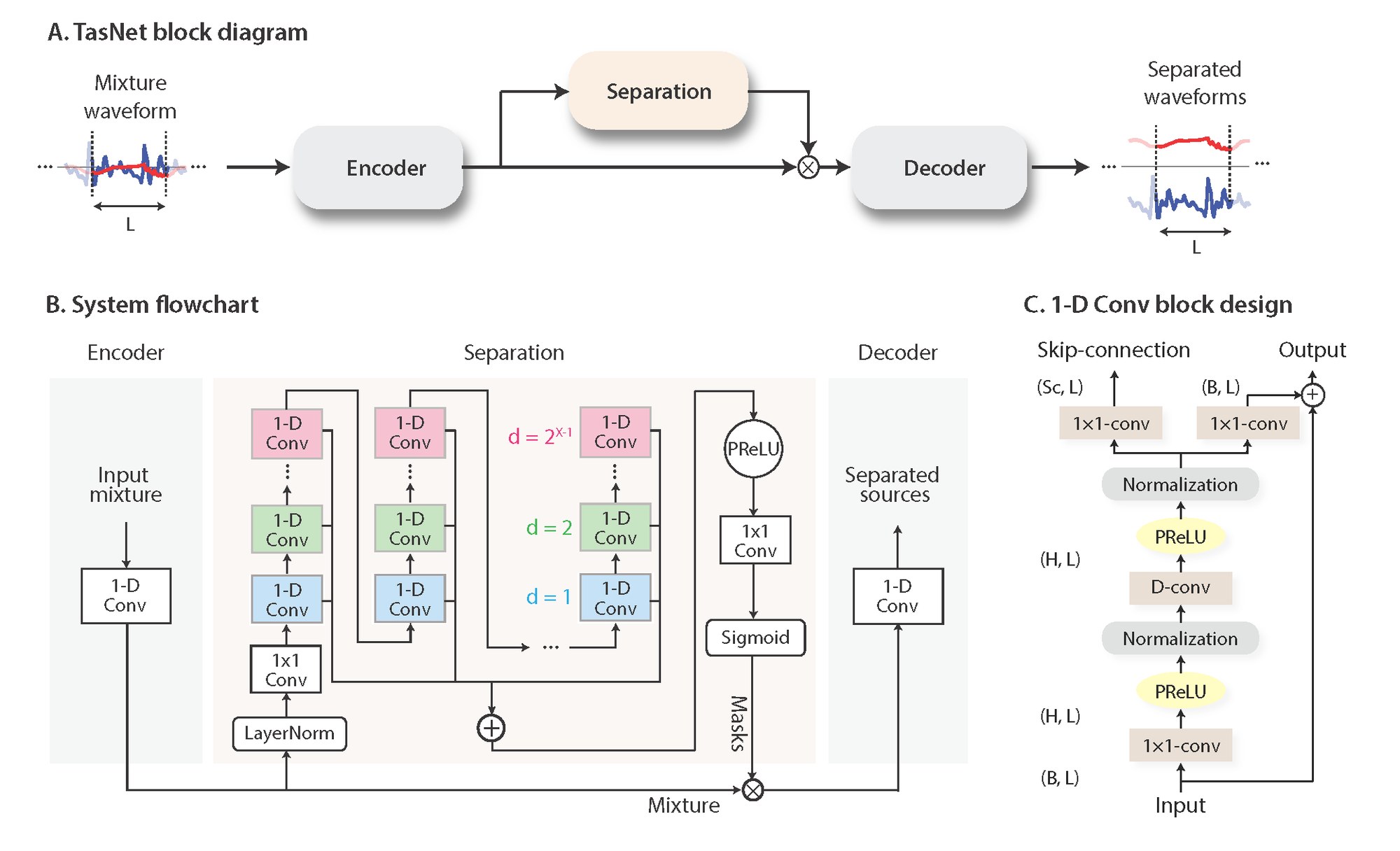
Fig. 1: (A): the block diagram of the TasNet system. An encoder maps a segment of the mixture waveform to a high-dimensional representation and a separation module calculates a multiplicative function (i.e., a mask) for each of the target sources. A decoder reconstructs the source waveforms from the masked features. (B): A flowchart of the proposed system. A 1-D convolutional autoencoder models the waveforms and a temporal convolutional network (TCN) separation module estimates the masks based on the encoder output. Different colors in the 1-D convolutional blocks in TCN denote different dilation factors. (C): The design of 1-D convolutional block. Each block consists of a $1\times 1\text{-}conv$ operation followed by a depthwise convolution ($D-conv$) operation, with nonlinear activation function and normalization added between each two convolution operations. Two linear $1\times 1{-}conv$ blocks serve as the residual path and the skip-connection path respectively.

图 1：（A）TasNet 系统的框图。编码器把一段混合波形映射到高维表示，分离模块为每个目标源计算一个乘法函数（即掩蔽）。解码器再从掩蔽后的特征重建源波形。（B）所提出系统的流程图。一维卷积自编码器对波形建模，时间卷积网络（TCN）分离模块根据编码器输出估计掩蔽。TCN 中一维卷积块的不同颜色表示不同的膨胀因子。（C）一维卷积块的设计。每个块由一次 $1\times 1\text{-}conv$ 运算后接一次深度卷积（$D-conv$）组成，并在每两次卷积运算之间加入非线性激活函数和归一化。两条线性的 $1\times 1{-}conv$ 路径分别作为残差路径和跳跃连接路径。

II-A Time-domain speech separation

II-A 时域语音分离

The problem of single-channel speech separation can be formulated in terms of estimating $C$ sources $s_{1}(t),\ldots,s_{c}(t)\in\mathbb{R}^{1\times T}$, given the discrete waveform of the mixture $x(t)\in\mathbb{R}^{1\times T}$, where

单通道语音分离问题可以表述为：在给定混合信号离散波形 $x(t)\in\mathbb{R}^{1\times T}$ 的条件下，估计 $C$ 个源 $s_{1}(t),\ldots,s_{c}(t)\in\mathbb{R}^{1\times T}$，其中

$$\displaystyle x(t)=\sum_{i=1}^{C}s_{i}(t) \tag{1}$$

In time-domain audio separation, we aim to directly estimate $s_{i}(t),i=1,\ldots,C$, from $x(t)$.

在时域音频分离中，我们的目标是直接从 $x(t)$ 估计 $s_{i}(t),i=1,\ldots,C$。

II-B Convolutional encoder-decoder

II-B 卷积编码器–解码器

The input mixture sound can be divided into overlapping segments of length $L$, represented by $\bm{\mathrm{x}}_{k}\in\mathbb{R}^{1\times L}$, where $k=1,\dots,\hat{T}$ denotes the segment index and $\hat{T}$ denotes the total number of segments in the input. $\bm{\mathrm{x}}_{k}$ is transformed into a $N$-dimensional representation, $\bm{\mathrm{w}}\in\mathbb{R}^{1\times N}$ by a 1-D convolution operation, which is reformulated as a matrix multiplication (the index $k$ is dropped from now on):

输入的混合声音可以分成长度为 $L$ 的重叠段，记为 $\bm{\mathrm{x}}_{k}\in\mathbb{R}^{1\times L}$，其中 $k=1,\dots,\hat{T}$ 是段的索引，$\hat{T}$ 是输入中段的总数。$\bm{\mathrm{x}}_{k}$ 通过一维卷积运算变换成 $N$ 维表示 $\bm{\mathrm{w}}\in\mathbb{R}^{1\times N}$，该运算被改写成矩阵乘法（此后略去下标 $k$）：

$$\displaystyle\bm{\mathrm{w}}=\mathcal{H}(\bm{\mathrm{x}}\bm{\mathrm{U}}) \tag{2}$$

where $\bm{\mathrm{U}}\in\mathbb{R}^{N\times L}$ contains $N$ vectors (encoder basis functions) with length $L$ each, and $\mathcal{H}(\cdot)$ is an optional nonlinear function. In [21, 26], $\mathcal{H}(\cdot)$ was the rectified linear unit (ReLU) to ensure that the representation is non-negative. The decoder reconstructs the waveform from this representation using a 1-D transposed convolution operation, which can be reformulated as another matrix multiplication:

其中 $\bm{\mathrm{U}}\in\mathbb{R}^{N\times L}$ 包含 $N$ 个向量（编码器基函数），每个长度为 $L$，$\mathcal{H}(\cdot)$ 是可选的非线性函数。在 [21, 26] 中，$\mathcal{H}(\cdot)$ 取整流线性单元（ReLU），以保证表示非负。解码器用一维转置卷积从这一表示重建波形，该运算同样可以改写成另一次矩阵乘法：

$$\displaystyle\hat{\bm{\mathrm{x}}}=\bm{\mathrm{w}}\bm{\mathrm{V}} \tag{3}$$

where $\hat{\bm{\mathrm{x}}}\in\mathbb{R}^{1\times L}$ is the reconstruction of $\bm{\mathrm{x}}$, and the rows in $\bm{\mathrm{V}}\in\mathbb{R}^{N\times L}$ are the decoder basis functions, each with length $L$. The overlapping reconstructed segments are summed together to generate the final waveforms.

其中 $\hat{\bm{\mathrm{x}}}\in\mathbb{R}^{1\times L}$ 是 $\bm{\mathrm{x}}$ 的重建，而 $\bm{\mathrm{V}}\in\mathbb{R}^{N\times L}$ 的各行是解码器基函数，每个长度为 $L$。重叠的重建段再相加，得到最终波形。

Although we reformulate the encoder/decoder operations as matrix multiplication, the term ”convolutional autoencoder” is used because in actual model implementation, convolutional and transposed convolutional layers can more easily handle the overlap between segments and thus enable faster training and better convergence. [^1]

虽然我们把编码器/解码器运算改写成了矩阵乘法，仍然使用“卷积自编码器”这一说法，因为在实际模型实现中，卷积层和转置卷积层能更方便地处理段与段之间的重叠，从而加快训练并改善收敛。[^1]

II-C Estimating the separation masks

II-C 估计分离掩蔽

The separation for each frame is performed by estimating $C$ vectors (masks) $\bm{\mathrm{m}}_{i}\in\mathbb{R}^{1\times N},i=1,\ldots,C$ where $C$ is the number of speakers in the mixture that is multiplied by the encoder output $\bm{\mathrm{w}}$. The mask vectors $\bm{\mathrm{m}}_{i}$ have the constraint that $\bm{\mathrm{m}}_{i}\in[0,1]$. The representation of each source, $\bm{\mathrm{d}}_{i}\in\mathbb{R}^{1\times N}$, is then calculated by applying the corresponding mask, $\bm{\mathrm{m}}_{i}$, to the mixture representation $\bm{\mathrm{w}}$:

每一帧的分离，是通过估计 $C$ 个向量（掩蔽）$\bm{\mathrm{m}}_{i}\in\mathbb{R}^{1\times N},i=1,\ldots,C$ 来完成的，其中 $C$ 是混合中的说话人数，这些向量再与编码器输出 $\bm{\mathrm{w}}$ 相乘。掩蔽向量 $\bm{\mathrm{m}}_{i}$ 满足约束 $\bm{\mathrm{m}}_{i}\in[0,1]$。每个源的表示 $\bm{\mathrm{d}}_{i}\in\mathbb{R}^{1\times N}$，再通过把相应掩蔽 $\bm{\mathrm{m}}_{i}$ 加到混合表示 $\bm{\mathrm{w}}$ 上计算得到：

$$\displaystyle\bm{\mathrm{d}}_{i}=\bm{\mathrm{w}}\odot\bm{\mathrm{m}}_{i} \tag{4}$$

where $\odot$ denotes element-wise multiplication. The waveform of each source $\hat{\bm{\mathrm{s}}}_{i},i=1,\ldots,C$ is then reconstructed by the decoder:

其中 $\odot$ 表示逐元素相乘。每个源的波形 $\hat{\bm{\mathrm{s}}}_{i},i=1,\ldots,C$ 再由解码器重建：

$$\displaystyle\hat{\bm{\mathrm{s}}}_{i}=\bm{\mathrm{d}}_{i}\bm{\mathrm{V}} \tag{5}$$

The unit summation constraint in [21, 26], $\sum_{i=1}^{C}\bm{\mathrm{m}}_{i}=\mathbb{\bm{\mathrm{1}}}$, was applied based on the assumption that the encoder-encoder architecture can perfectly reconstruct the input mixture. In section IV-A, we will examine the consequence of relaxing this unity summation constraint on separation accuracy.

文献 [21, 26] 中的单位求和约束 $\sum_{i=1}^{C}\bm{\mathrm{m}}_{i}=\mathbb{\bm{\mathrm{1}}}$，是基于编码器–编码器结构能够完美重建输入混合这一假定而施加的。在第 IV-A 节中，我们将考察放宽这一单位求和约束对分离精度的影响。

II-D Convolutional separation module

II-D 卷积分离模块

Motivated by the temporal convolutional network (TCN) [29, 30, 31], we propose a fully-convolutional separation module that consists of stacked 1-D dilated convolutional blocks, as shown in figure 1 (B). TCN was proposed as a replacement for RNNs in various sequence modeling tasks. Each layer in a TCN consists of 1-D convolutional blocks with increasing dilation factors. The dilation factors increase exponentially to ensure a sufficiently large temporal context window to take advantage of the long-range dependencies of the speech signal, as denoted with different colors in figure 1 (B). In Conv-TasNet, $M$ convolutional blocks with dilation factors $1,2,4,\ldots,2^{M-1}$ are repeated $R$ times. The input to each block is zero padded accordingly to ensure the output length is the same as the input. The output of the TCN is passed to a convolutional block with kernel size $1$ ($1\times 1{-}conv$ block, also known as pointwise convolution) for mask estimation. The $1\times 1{-}conv$ block together with a nonlinear activation function estimates $C$ mask vectors for the $C$ target sources.

受时间卷积网络（TCN）[29, 30, 31] 的启发，我们提出一个全卷积的分离模块，由堆叠的一维膨胀卷积块组成，如图 1（B）所示。TCN 被提出来作为各类序列建模任务中 RNN 的替代。TCN 的每一层由膨胀因子递增的一维卷积块组成。膨胀因子按指数增加，以保证足够大的时间上下文窗口，从而利用语音信号的长程依赖，图 1（B）中用不同颜色标出。在 Conv-TasNet 中，膨胀因子为 $1,2,4,\ldots,2^{M-1}$ 的 $M$ 个卷积块重复 $R$ 次。每个块的输入会做相应的零填充，以保证输出长度与输入相同。TCN 的输出再送入核尺寸为 $1$ 的卷积块（$1\times 1{-}conv$ 块，也称 逐点 卷积）来估计掩蔽。该 $1\times 1{-}conv$ 块与非线性激活函数一起，为 $C$ 个目标源估计 $C$ 个掩蔽向量。

Figure 1 (C) shows the design of each 1-D convolutional block. The design of the 1-D convolutional blocks follows [38], where a residual path and a skip-connection path are applied: the residual path of a block serves as the input to the next block, and the skip-connection paths for all blocks are summed up and used as the output of the TCN. To further decrease the number of parameters, depthwise separable convolution ($S\text{-}conv(\cdot)$) is used to replace standard convolution in each convolutional block. Depthwise separable convolution (also referred to as separable convolution) has proven effective in image processing tasks [32, 33] and neural machine translation tasks [39]. The depthwise separable convolution operator decouples the standard convolution operation into two consecutive operations, a depthwise convolution ($D\text{-}conv(\cdot)$) followed by pointwise convolution ($1\times 1{-}conv(\cdot)$):

图 1（C）给出了每个一维卷积块的设计。一维卷积块的设计沿用 [38]，其中使用了残差路径和跳跃连接路径：一个块的残差路径作为下一块的输入，所有块的跳跃连接路径相加后作为 TCN 的输出。为了进一步减少参数量，每个卷积块中的标准卷积被换成深度可分离卷积（$S\text{-}conv(\cdot)$）。深度可分离卷积（也称可分离卷积）已在图像处理任务 [32, 33] 和神经机器翻译任务 [39] 中被证明有效。深度可分离卷积算子把标准卷积拆成两次相继的运算，即深度卷积（$D\text{-}conv(\cdot)$）后接逐点卷积（$1\times 1{-}conv(\cdot)$）：

$$\displaystyle D\text{-}conv(\bm{\mathrm{Y}},\bm{\mathrm{K}}) \\ \displaystyle=concat(\bm{\mathrm{y}}_{j}\circledast\bm{\mathrm{k}}_{j}),j=1,\ldots,N \\ \displaystyle S\text{-}conv(\bm{\mathrm{Y}},\bm{\mathrm{K}},\bm{\mathrm{L}}) \\ \displaystyle=D\text{-}conv(\bm{\mathrm{Y}},\bm{\mathrm{K}})\circledast\bm{\mathrm{L}} \tag{6}$$

where $\bm{\mathrm{Y}}\in\mathbb{R}^{G\times M}$ is the input to $S\text{-}conv(\cdot)$, $\bm{\mathrm{K}}\in\mathbb{R}^{G\times P}$ is the convolution kernel with size $P$, $\bm{\mathrm{y}}_{j}\in\mathbb{R}^{1\times M}$ and $\bm{\mathrm{k}}_{j}\in\mathbb{R}^{1\times P}$ are the rows of matrices $\bm{\mathrm{Y}}$ and $\bm{\mathrm{K}}$, respectively, $\bm{\mathrm{L}}\in\mathbb{R}^{G\times H\times 1}$ is the convolution kernel with size 1, and $\circledast$ denotes the convolution operation. In other words, the $D\text{-}conv(\cdot)$ operation convolves each row of the input $Y$ with the corresponding row of matrix $K$, and the $1\times 1{-}conv$ block linearly transforms the feature space. In comparison with the standard convolution with kernel size $\hat{\bm{\mathrm{K}}}\in\mathbb{R}^{G\times H\times P}$, depthwise separable convolution only contains $G\times P+G\times H$ parameters, which decreases the model size by a factor of $\frac{H\times P}{H+P}\approx P$ when $H\gg P$.

其中 $\bm{\mathrm{Y}}\in\mathbb{R}^{G\times M}$ 是 $S\text{-}conv(\cdot)$ 的输入，$\bm{\mathrm{K}}\in\mathbb{R}^{G\times P}$ 是尺寸为 $P$ 的卷积核，$\bm{\mathrm{y}}_{j}\in\mathbb{R}^{1\times M}$ 和 $\bm{\mathrm{k}}_{j}\in\mathbb{R}^{1\times P}$ 分别是矩阵 $\bm{\mathrm{Y}}$ 和 $\bm{\mathrm{K}}$ 的行，$\bm{\mathrm{L}}\in\mathbb{R}^{G\times H\times 1}$ 是尺寸为 1 的卷积核，$\circledast$ 表示卷积运算。换句话说，$D\text{-}conv(\cdot)$ 运算用矩阵 $K$ 的相应行去卷积输入 $Y$ 的每一行，而 $1\times 1{-}conv$ 块对特征空间做线性变换。与核为 $\hat{\bm{\mathrm{K}}}\in\mathbb{R}^{G\times H\times P}$ 的标准卷积相比，深度可分离卷积只包含 $G\times P+G\times H$ 个参数，在 $H\gg P$ 时可以把模型规模缩小约 $\frac{H\times P}{H+P}\approx P$ 倍。

A nonlinear activation function and a normalization operation are added after both the first $1\times 1\text{-}conv$ and $D\text{-}conv$ blocks respectively. The nonlinear activation function is the parametric rectified linear unit (PReLU) [40]:

在第一个 $1\times 1\text{-}conv$ 块和 $D\text{-}conv$ 块之后，分别加入非线性激活函数和归一化运算。非线性激活函数采用参数化整流线性单元（PReLU）[40]：

$$\displaystyle PReLU(x)=\begin{cases}x,\quad\text{if},x\geq 0\
\alpha x,\quad\text{otherwise}\end{cases} \tag{8}$$

$$\displaystyle PReLU(x)=\begin{cases}x,\quad\text{if}\,x\geq 0\\ \alpha x,\quad\text{otherwise}\end{cases} \tag{8}$$

where $\alpha\in\mathbb{R}$ is a trainable scalar controlling the negative slope of the rectifier. The choice of the normalization method in the network depends on the causality requirement. For noncausal configuration, we found empirically that global layer normalization (gLN) outperforms all other normalization methods. In gLN, the feature is normalized over both the channel and the time dimensions:

其中 $\alpha\in\mathbb{R}$ 是可训练的标量，用来控制整流器的负斜率。网络中归一化方法的选择取决于对因果性的要求。对非因果配置，我们从经验上发现全局层归一化（gLN）优于其他所有归一化方法。在 gLN 中，特征在通道维和时间维上同时做归一化：

$$\displaystyle gLN(\bm{\mathrm{F}}) \\ \displaystyle=\frac{\bm{\mathrm{F}}-E[\bm{\mathrm{F}}]}{\sqrt{Var[\bm{\mathrm{F}}]+\epsilon}}\odot\gamma+\beta \\ \displaystyle E[\bm{\mathrm{F}}] \\ \displaystyle=\frac{1}{NT}\sum_{NT}{\bm{\mathrm{F}}} \\ \displaystyle Var[\bm{\mathrm{F}}] \\ \displaystyle=\frac{1}{NT}\sum_{NT}{(\bm{\mathrm{F}}-E[\bm{\mathrm{F}}])^{2}} \tag{9}$$

where $\bm{\mathrm{F}}\in\mathbb{R}^{N\times T}$ is the feature, $\gamma,\beta\in\mathbb{R}^{N\times 1}$ are trainable parameters, and $\epsilon$ is a small constant for numerical stability. This is identical to the standard layer normalization applied in computer vision models where the channel and time dimension correspond to the width and height dimension in an image [41]. In causal configuration, gLN cannot be applied since it relies on the future values of the signal at any time step. Instead, we designed a cumulative layer normalization (cLN) operation to perform step-wise normalization in the causal system:

其中 $\bm{\mathrm{F}}\in\mathbb{R}^{N\times T}$ 是特征，$\gamma,\beta\in\mathbb{R}^{N\times 1}$ 是可训练参数，$\epsilon$ 是为数值稳定而设的小常数。这与计算机视觉模型中常用的标准层归一化相同，只是通道维和时间维对应于图像中的宽度和高度维 [41]。在因果配置下，gLN 不能使用，因为它在任一时间步都依赖于信号的未来取值。我们因而设计了累积层归一化（cLN）运算，以便在因果系统中做逐步归一化：

$$\displaystyle cLN(\bm{\mathrm{f}}_{k}) \\ \displaystyle=\frac{\bm{\mathrm{f}}_{k}-E[\bm{\mathrm{f}}_{t\leq k}]}{\sqrt{Var[\bm{\mathrm{f}}_{t\leq k}]+\epsilon}}\odot\gamma+\beta \\ \displaystyle E[\bm{\mathrm{f}}_{t\leq k}] \\ \displaystyle=\frac{1}{Nk}\sum_{Nk}{\bm{\mathrm{f}}_{t\leq k}} \\ \displaystyle Var[\bm{\mathrm{f}}_{t\leq k}] \\ \displaystyle=\frac{1}{Nk}\sum_{Nk}{(\bm{\mathrm{f}}_{t\leq k}-E[\bm{\mathrm{f}}_{t\leq k}])^{2}} \tag{12}$$

where $\bm{\mathrm{f}}_{k}\in\mathbb{R}^{N\times 1}$ is the $k$-th frame of the entire feature $\bm{\mathrm{F}}$, $\bm{\mathrm{f}}_{t\leq k}\in\mathbb{R}^{N\times k}$ corresponds to the feature of $k$ frames $[\bm{\mathrm{f}}_{1},\ldots,\bm{\mathrm{f}}_{k}]$, and $\gamma,\beta\in\mathbb{R}^{N\times 1}$ are trainable parameters applied to all frames. To ensure that the separation module is invariant to the scaling of the input, the selected normalization method is applied to the encoder output $\bm{\mathrm{w}}$ before it is passed to the separation module.

其中 $\bm{\mathrm{f}}_{k}\in\mathbb{R}^{N\times 1}$ 是整段特征 $\bm{\mathrm{F}}$ 的第 $k$ 帧，$\bm{\mathrm{f}}_{t\leq k}\in\mathbb{R}^{N\times k}$ 对应 $k$ 帧特征 $[\bm{\mathrm{f}}_{1},\ldots,\bm{\mathrm{f}}_{k}]$，$\gamma,\beta\in\mathbb{R}^{N\times 1}$ 是应用于所有帧的可训练参数。为了使分离模块对输入的尺度保持不变，所选用的归一化方法会先施加到编码器输出 $\bm{\mathrm{w}}$ 上，再送入分离模块。

At the beginning of the separation module, a linear $1\times 1\text{-}conv$ block is added as a bottleneck layer. This block determines the number of channels in the input and residual path of the subsequent convolutional blocks. For instance, if the linear bottleneck layer has $B$ channels, then for a 1-D convolutional block with $H$ channels and kernel size $P$, the size of the kernel in the first $1\times 1\text{-}conv$ block and the first $D\text{-}conv$ block should be $\bm{\mathrm{O}}\in\mathbb{R}^{B\times H\times 1}$ and $\bm{\mathrm{K}}\in\mathbb{R}^{H\times P}$ respectively, and the size of the kernel in the residual paths should be $\bm{\mathrm{L}}_{Rs}\in\mathbb{R}^{H\times B\times 1}$. The number of output channels in the skip-connection path can be different than $B$, and we denote the size of kernels in that path as $\bm{\mathrm{L}}_{Sc}\in\mathbb{R}^{H\times Sc\times 1}$.

在分离模块的开头，加入一个线性的 $1\times 1\text{-}conv$ 块作为瓶颈层。该块决定后续卷积块输入和残差路径中的通道数。例如，若线性瓶颈层有 $B$ 个通道，那么对于通道数为 $H$、核尺寸为 $P$ 的一维卷积块，第一个 $1\times 1\text{-}conv$ 块和第一个 $D\text{-}conv$ 块中核的尺寸应分别为 $\bm{\mathrm{O}}\in\mathbb{R}^{B\times H\times 1}$ 和 $\bm{\mathrm{K}}\in\mathbb{R}^{H\times P}$，残差路径中核的尺寸应为 $\bm{\mathrm{L}}_{Rs}\in\mathbb{R}^{H\times B\times 1}$。跳跃连接路径的输出通道数可以与 $B$ 不同，我们把该路径中核的尺寸记为 $\bm{\mathrm{L}}_{Sc}\in\mathbb{R}^{H\times Sc\times 1}$。

III Experimental procedures

III 实验步骤

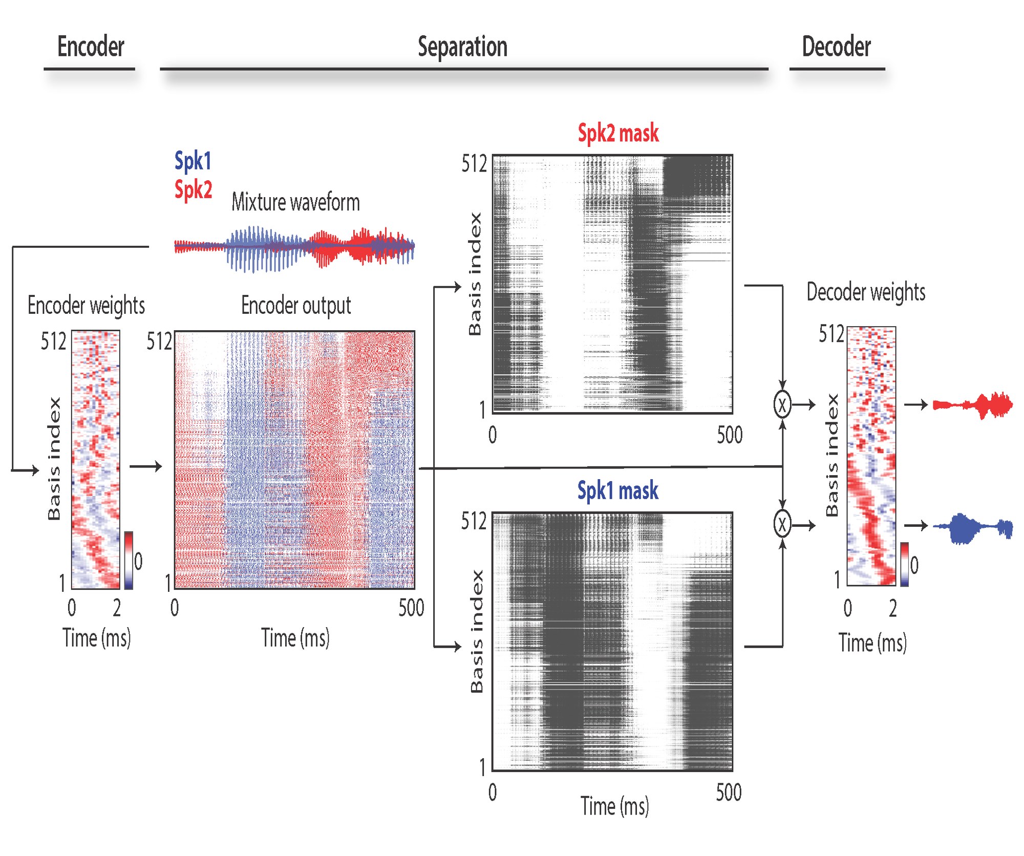
Fig. 2: Visualization of the encoder and decoder basis functions, encoder representation, and source masks for a sample 2-speaker mixture. The speakers are shown in red and blue. The encoder representation is colored according to the power of each speaker at each basis function and point in time. The basis functions are sorted according to their Euclidean similarity and show diversity in frequency and phase tuning.

图 2：对一个两说话人混合样本，可视化编码器与解码器的基函数、编码器表示以及源掩蔽。两个说话人分别用红色和蓝色标出。编码器表示按每个基函数、每个时间点上各说话人的功率着色。基函数按欧氏相似度排序，在频率和相位调谐上呈现出多样性。

III-A Dataset

III-A 数据集

We evaluated our system on two-speaker and three-speaker speech separation problems using the WSJ0-2mix and WSJ0-3mix datasets [25]. 30 hours of training and 10 hours of validation data are generated from speakers in si_tr_s from the datasets. The speech mixtures are generated by randomly selecting utterances from different speakers in the Wall Street Journal dataset (WSJ0) and mixing them at random signal-to-noise ratios (SNR) between -5 dB and 5 dB. 5 hours of evaluation set is generated in the same way using utterances from 16 unseen speakers in si_dt_05 and si_et_05. The scripts for creating the dataset can be found at [42]. All the waveforms are resampled at 8 kHz.

我们在两说话人和三说话人语音分离问题上评估系统，数据采用 WSJ0-2mix 和 WSJ0-3mix 数据集 [25]。30 小时训练数据和 10 小时验证数据由数据集中 si_tr_s 的说话人生成。语音混合的做法是：从华尔街日报语料（WSJ0）中随机选取不同说话人的语句，并按 $-5$ 分贝到 $5$ 分贝之间的随机信噪比（SNR）混合。5 小时评价集用同样方式生成，语句来自 si_dt_05 和 si_et_05 中 16 位未见过的说话人。创建该数据集的脚本见 [42]。所有波形均以 8 kHz 重采样。

III-B Experiment configurations

III-B 实验配置

The networks are trained for 100 epochs on 4-second long segments. The initial learning rate is set to $1e^{-3}$. The learning rate is halved if the accuracy of validation set is not improved in 3 consecutive epochs. Adam [43] is used as the optimizer. A 50% stride size is used in the convolutional autoencoder (i.e. 50% overlap between consecutive frames). Gradient clipping with maximum $L_{2}$-norm of 5 is applied during training. The hyperparameters of the network are shown in table I. A Pytorch implementation of the Conv-TasNet model can be found at [^2].

网络在 4 秒长的片段上训练 100 个周期。初始学习率设为 $1e^{-3}$。若验证集精度连续 3 个周期没有提高，学习率减半。优化器采用 Adam [43]。卷积自编码器使用 50% 的步长（即相邻帧之间重叠 50%）。训练时施加梯度裁剪，最大 $L_{2}$ 范数为 5。网络的超参数见表 I。Conv-TasNet 模型的 Pytorch 实现见 [^2]。

Symbol	Description
$N$	Number of filters in autoencoder
$L$	Length of the filters (in samples)
$B$	Number of channels in bottleneck and the residual paths’ $1\times 1\text{-}conv$ blocks
$Sc$	Number of channels in skip-connection paths’ $1\times 1\text{-}conv$ blocks
$H$	Number of channels in convolutional blocks
$P$	Kernel size in convolutional blocks
$X$	Number of convolutional blocks in each repeat
$R$	Number of repeats

TABLE I: Hyperparameters of the network.

符号	说明
$N$	自编码器中的滤波器数量
$L$	滤波器长度（以样本计）
$B$	瓶颈路径以及残差路径上 $1\times 1\text{-}conv$ 块的通道数
$Sc$	跳跃连接路径上 $1\times 1\text{-}conv$ 块的通道数
$H$	卷积块中的通道数
$P$	卷积块中的核尺寸
$X$	每一重复中的卷积块数量
$R$	重复次数

表 I：网络的超参数。

III-C Training objective

III-C 训练目标

The objective of training the end-to-end system is maximizing the scale-invariant source-to-noise ratio (SI-SNR), which has commonly been used as the evaluation metric for source separation replacing the standard source-to-distortion ratio (SDR) [44, 5, 9]. SI-SNR is defined as:

端到端系统的训练目标是最大化尺度不变信噪比（SI-SNR）。这一指标已常被用来替代标准的信号失真比（SDR），作为源分离的评价指标 [44, 5, 9]。SI-SNR 定义为：

$$\displaystyle\begin{cases}\bm{\mathrm{s}}{target}:=\frac{\langle\hat{\bm{\mathrm{s}}},\bm{\mathrm{s}}\rangle\bm{\mathrm{s}}}{\left|\bm{\mathrm{s}}\right|^{2}}\
\bm{\mathrm{e}}{noise}:=\hat{\bm{\mathrm{s}}}-\bm{\mathrm{s}}{target}\
\text{SI-SNR}:=10,log{10}\frac{\left|\bm{\mathrm{s}}{target}\right|^{2}}{\left|\bm{\mathrm{e}}{noise}\right|^{2}}\end{cases} \tag{15}$$

$$\displaystyle\begin{cases}\bm{\mathrm{s}}_{target}:=\frac{\langle\hat{\bm{\mathrm{s}}},\bm{\mathrm{s}}\rangle\bm{\mathrm{s}}}{\left\|\bm{\mathrm{s}}\right\|^{2}}\\ \bm{\mathrm{e}}_{noise}:=\hat{\bm{\mathrm{s}}}-\bm{\mathrm{s}}_{target}\\ \text{SI-SNR}:=10\,log_{10}\frac{\left\|\bm{\mathrm{s}}_{target}\right\|^{2}}{\left\|\bm{\mathrm{e}}_{noise}\right\|^{2}}\end{cases} \tag{15}$$

where $\hat{\bm{\mathrm{s}}}\in\mathbb{R}^{1\times T}$ and $\bm{\mathrm{s}}\in\mathbb{R}^{1\times T}$ are the estimated and original clean sources, respectively, and $\left\|\bm{\mathrm{s}}\right\|^{2}=\langle\bm{\mathrm{s}},\bm{\mathrm{s}}\rangle$ denotes the signal power. Scale invariance is ensured by normalizing $\hat{\bm{\mathrm{s}}}$ and $\bm{\mathrm{s}}$ to zero-mean prior to the calculation. Utterance-level permutation invariant training (uPIT) is applied during training to address the source permutation problem [7].

其中 $\hat{\bm{\mathrm{s}}}\in\mathbb{R}^{1\times T}$ 和 $\bm{\mathrm{s}}\in\mathbb{R}^{1\times T}$ 分别是估计源和原来的干净源，$\left\|\bm{\mathrm{s}}\right\|^{2}=\langle\bm{\mathrm{s}},\bm{\mathrm{s}}\rangle$ 表示信号功率。尺度不变性通过在计算前把 $\hat{\bm{\mathrm{s}}}$ 和 $\bm{\mathrm{s}}$ 归一化到零均值来保证。训练时采用语句级置换不变训练（uPIT）来处理源的排列问题 [7]。

III-D Evaluation metrics

III-D 评价指标

We report the scale-invariant signal-to-noise ratio improvement (SI-SNRi) and signal-to-distortion ratio improvement (SDRi) [44] as objective measures of separation accuracy. SI-SNR is defined in equation 15. The reported improvements in tables III to V indicate the additive values over the original mixture. In addition to the distortion metrics, we also evaluated the quality of the separated mixtures using both the perceptual evaluation of subjective quality (PESQ, [45]) and the mean opinion score (MOS) [46] by asking 40 normal hearing subjects to rate the quality of the separated mixtures. All human testing procedures were approved by the local institutional review board (IRB) at Columbia University in the City of New York.

我们报告尺度不变信噪比提升（SI-SNRi）和信号失真比提升（SDRi）[44]，作为分离精度的客观指标。SI-SNR 的定义见公式 15。表 III 至表 V 中报告的提升，是相对原始混合的附加值。除了失真指标，我们还用感知语音质量评价（PESQ，[45]）以及平均意见分（MOS）[46] 来评估分离后混合的质量，做法是请 40 名听力正常的受试者对分离后混合的质量打分。所有人体测试程序均已通过纽约市哥伦比亚大学当地机构审查委员会（IRB）批准。

III-E Comparison with ideal time-frequency masks

III-E 与理想时频掩蔽的比较

Following the common configurations in [5, 9, 7], the ideal time-frequency masks were calculated using STFT with a 32 ms window size and 8 ms hop size with a Hanning window. The ideal masks include the ideal binary mask (IBM), ideal ratio mask (IRM), and Wiener filter-like mask (WFM), which are defined for source $i$ as:

按照 [5, 9, 7] 中的常用配置，理想时频掩蔽用窗长 32 毫秒、帧移 8 毫秒、并加汉宁窗的 STFT 计算。理想掩蔽包括理想二值掩蔽（IBM）、理想比值掩蔽（IRM）和类维纳滤波掩蔽（WFM），对源 $i$ 分别定义为：

$$\displaystyle IBM_{i}(f,t) \ \displaystyle=\begin{cases}1,,\left|\mathcal{S}{i}(f,t)\right|>\left|\mathcal{S}{j\neq i}(f,t)\right|\
0,,\text{otherwise}\end{cases} \ \displaystyle IRM_{i}(f,t) \ \displaystyle=\frac{\left|\mathcal{S}{i}(f,t)\right|}{\sum{j=1}^{C}\left|\mathcal{S}{j}(f,t)\right|} \ \displaystyle WFM{i}(f,t) \ \displaystyle=\frac{\left|\mathcal{S}{i}(f,t)\right|^{2}}{\sum{j=1}^{C}\left|\mathcal{S}_{j}(f,t)\right|^{2}} \tag{16}$$

$$\displaystyle IBM_{i}(f,t) \\ \displaystyle=\begin{cases}1,\,\left|\mathcal{S}_{i}(f,t)\right|>\left|\mathcal{S}_{j\neq i}(f,t)\right|\\ 0,\,\text{otherwise}\end{cases} \\ \displaystyle IRM_{i}(f,t) \\ \displaystyle=\frac{\left|\mathcal{S}_{i}(f,t)\right|}{\sum_{j=1}^{C}\left|\mathcal{S}_{j}(f,t)\right|} \\ \displaystyle WFM_{i}(f,t) \\ \displaystyle=\frac{\left|\mathcal{S}_{i}(f,t)\right|^{2}}{\sum_{j=1}^{C}\left|\mathcal{S}_{j}(f,t)\right|^{2}} \tag{16}$$

where $\mathcal{S}_{i}(f,t)\in\mathbb{C}^{F\times T}$ are the complex-valued spectrograms of clean sources $i=1,\ldots,C$.

其中 $\mathcal{S}_{i}(f,t)\in\mathbb{C}^{F\times T}$ 是干净源 $i=1,\ldots,C$ 的复数值语谱图。

IV Results

IV 结果

$N$	$L$	$B$	$H$	$Sc$	$P$	$X$	$R$	Normalization	Causal	Receptive field (s)	Model size	SI-SNRi (dB)	SDRi (dB)
128	40	128	256	128	3	7	2	gLN	×	1.28	1.5M	13.0	13.3
256	40	128	256	128	3	7	2	gLN	×	1.28	1.5M	13.1	13.4
512	40	128	256	128	3	7	2	gLN	×	1.28	1.7M	13.3	13.6
512	40	128	256	256	3	7	2	gLN	×	1.28	2.4M	13.0	13.3
512	40	128	512	128	3	7	2	gLN	×	1.28	3.1M	13.3	13.6
512	40	128	512	512	3	7	2	gLN	×	1.28	6.2M	13.5	13.8
512	40	256	256	256	3	7	2	gLN	×	1.28	3.2M	13.0	13.3
512	40	256	512	256	3	7	2	gLN	×	1.28	6.0M	13.4	13.7
512	40	256	512	512	3	7	2	gLN	×	1.28	8.1M	13.2	13.5
512	40	128	512	128	3	6	4	gLN	×	1.27	5.1M	14.1	14.4
512	40	128	512	128	3	4	6	gLN	×	0.46	5.1M	13.9	14.2
512	40	128	512	128	3	8	3	gLN	×	3.83	5.1M	14.5	14.8
512	32	128	512	128	3	8	3	gLN	×	3.06	5.1M	14.7	15.0
512	16	128	512	128	3	8	3	gLN	×	1.53	5.1M	15.3	15.6
512	16	128	512	128	3	8	3	cLN	✓	1.53	5.1M	10.6	11.0

TABLE II: The effect of different configurations in Conv-TasNet.

$N$	$L$	$B$	$H$	$Sc$	$P$	$X$	$R$	归一化	因果	感受野（秒）	模型规模	SI-SNRi（分贝）	SDRi（分贝）
128	40	128	256	128	3	7	2	gLN	×	1.28	1.5M	13.0	13.3
256	40	128	256	128	3	7	2	gLN	×	1.28	1.5M	13.1	13.4
512	40	128	256	128	3	7	2	gLN	×	1.28	1.7M	13.3	13.6
512	40	128	256	256	3	7	2	gLN	×	1.28	2.4M	13.0	13.3
512	40	128	512	128	3	7	2	gLN	×	1.28	3.1M	13.3	13.6
512	40	128	512	512	3	7	2	gLN	×	1.28	6.2M	13.5	13.8
512	40	256	256	256	3	7	2	gLN	×	1.28	3.2M	13.0	13.3
512	40	256	512	256	3	7	2	gLN	×	1.28	6.0M	13.4	13.7
512	40	256	512	512	3	7	2	gLN	×	1.28	8.1M	13.2	13.5
512	40	128	512	128	3	6	4	gLN	×	1.27	5.1M	14.1	14.4
512	40	128	512	128	3	4	6	gLN	×	0.46	5.1M	13.9	14.2
512	40	128	512	128	3	8	3	gLN	×	3.83	5.1M	14.5	14.8
512	32	128	512	128	3	8	3	gLN	×	3.06	5.1M	14.7	15.0
512	16	128	512	128	3	8	3	gLN	×	1.53	5.1M	15.3	15.6
512	16	128	512	128	3	8	3	cLN	✓	1.53	5.1M	10.6	11.0

表 II：Conv-TasNet 中不同配置的影响。

Figure 2 visualizes all the internal variables of Conv-TasNet for one example mixture sound with two overlapping speakers (denoted by red and blue). The encoder and decoder basis functions are sorted by the similarity of the Euclidean distance of the basis functions found using the unweighted pair group method with arithmetic mean (UPGMA) method [47]. The basis functions show a diversity of frequency and phase tuning. The representation of the encoder is colored according to the power of each speaker at the corresponding basis output at each time point, demonstrating the sparsity of the encoder representation. As can be seen in figure 2, the estimated masks for the two speakers highly resemble their encoder representations, which allows for the suppression of the encoder outputs that correspond to the interfering speaker and the extraction of the target speaker in each mask. The separated waveforms for the two speakers are estimated by the linear decoder, whose basis functions are shown in figure 2. The separated waveforms are shown on the right.

图 2 给出了 Conv-TasNet 对一个两说话人重叠混合样本（分别用红色和蓝色标出）的全部内部变量。编码器和解码器的基函数按基函数欧氏距离的相似度、用非加权组平均法（UPGMA）[47] 排序。这些基函数在频率和相位调谐上呈现出多样性。编码器表示按相应基输出在各时间点上每个说话人的功率着色，显示出编码器表示的稀疏性。如图 2 所示，两个说话人的估计掩蔽与他们的编码器表示高度相似，从而能够压低对应干扰说话人的编码器输出，并在各自掩蔽中提取目标说话人。两个说话人的分离波形由线性解码器估计，其基函数也示于图 2。分离后的波形显示在右侧。

IV-A Non-negativity of the encoder output

IV-A 编码器输出的非负性

The non-negativity of the encoder output was enforced in [21, 26] using a rectified-linear nonlinearity (ReLU) function. This constraint was based on the assumption that the masking operation on the encoder output is only meaningful when the mixture and speaker waveforms can be represented with a non-negative combination of the basis functions, since an unbounded encoder representation may result in unbounded masks. However, by removing the nonlinear function $\mathcal{H}$, another assumption can be made: with an unbounded but highly overcomplete representation of the mixture, a set of non-negative masks can still be found to reconstruct the clean sources. In this case, the overcompleteness of the representation is crucial. If there exist only a unique weight feature for the mixture as well as for the sources, the non-negativity of the mask cannot be guaranteed. Also note that in both assumptions, we put no constraint on the relationship between the encoder and decoder basis functions $\bm{\mathrm{U}}$ and $\bm{\mathrm{V}}$, meaning that they are not forced to reconstruct the mixture signal perfectly. One way to explicitly ensure the autoencoder property is by choosing $\bm{\mathrm{V}}$ to be the pseudo-inverse of $\bm{\mathrm{U}}$ (i.e. least square reconstruction). The choice of encoder/decoder design affects the mask estimation: in the case of an autoencoder, the unit summation constraint must be satisfied; otherwise, the unit summation constraint is not strictly required. To illustrate this point, we compared five different encoder-decoder configurations:

文献 [21, 26] 用整流线性非线性（ReLU）函数强制编码器输出非负。这一约束基于如下假定：只有当混合波形和说话人波形都能写成基函数的非负组合时，对编码器输出做掩蔽才有意义，因为无界的编码器表示可能导致无界的掩蔽。不过，若去掉非线性函数 $\mathcal{H}$，还可以做另一种假定：即使混合的表示无界但高度过完备，仍然可以找到一组非负掩蔽来重建干净源。在这种情况下，表示的过完备性至关重要。如果混合以及各源都只有唯一的权重特征，就不能保证掩蔽非负。还需要注意，在两种假定下，我们都没有对编码器与解码器基函数 $\bm{\mathrm{U}}$ 和 $\bm{\mathrm{V}}$ 的关系施加约束，也就是并不强迫它们完美重建混合信号。一种显式保证自编码器性质的办法，是取 $\bm{\mathrm{V}}$ 为 $\bm{\mathrm{U}}$ 的伪逆（即最小二乘重建）。编码器/解码器设计的选择会影响掩蔽估计：在自编码器的情形下，必须满足单位求和约束；否则，单位求和约束并不是严格必需的。为了说明这一点，我们比较了五种不同的编码器–解码器配置：

1. Linear encoder with its pseudo-inverse (Pinv) as decoder, i.e. $\bm{\mathrm{w}}=\bm{\mathrm{x}}(\bm{\mathrm{V}}^{T}\bm{\mathrm{V}})^{-1}\bm{\mathrm{V}}^{T}$ and $\hat{\bm{\mathrm{x}}}=\bm{\mathrm{w}}\bm{\mathrm{V}}$, with Softmax function for mask estimation.

1. 线性编码器，以其伪逆（Pinv）作为解码器，即 $\bm{\mathrm{w}}=\bm{\mathrm{x}}(\bm{\mathrm{V}}^{T}\bm{\mathrm{V}})^{-1}\bm{\mathrm{V}}^{T}$ 且 $\hat{\bm{\mathrm{x}}}=\bm{\mathrm{w}}\bm{\mathrm{V}}$，掩蔽估计使用 Softmax 函数。

2. Linear encoder and decoder where $\bm{\mathrm{w}}=\bm{\mathrm{x}}\bm{\mathrm{U}}$ and $\hat{\bm{\mathrm{x}}}=\bm{\mathrm{w}}\bm{\mathrm{V}}$, with Softmax or Sigmoid function for mask estimation.

2. 线性编码器与解码器，其中 $\bm{\mathrm{w}}=\bm{\mathrm{x}}\bm{\mathrm{U}}$ 且 $\hat{\bm{\mathrm{x}}}=\bm{\mathrm{w}}\bm{\mathrm{V}}$，掩蔽估计使用 Softmax 或 Sigmoid 函数。

3. Encoder with ReLU activation and linear decoder where $\bm{\mathrm{w}}=ReLU(\bm{\mathrm{x}}\bm{\mathrm{U}})$ and $\hat{\bm{\mathrm{x}}}=\bm{\mathrm{w}}\bm{\mathrm{V}}$, with Softmax or Sigmoid function for mask estimation.

3. 带 ReLU 激活的编码器与线性解码器，其中 $\bm{\mathrm{w}}=ReLU(\bm{\mathrm{x}}\bm{\mathrm{U}})$ 且 $\hat{\bm{\mathrm{x}}}=\bm{\mathrm{w}}\bm{\mathrm{V}}$，掩蔽估计使用 Softmax 或 Sigmoid 函数。

Separation accuracy of different configurations in table III shows that pseudo-inverse autoencoder leads to the worst performance, indicating that an explicit autoencoder configuration does not necessarily improve the separation score in this framework. The performance of all other configurations is comparable. Because linear encoder and decoder with Sigmoid function achieves a slightly better accuracy over other methods, we used this configuration in all the following experiments.

表 III 中不同配置的分离精度表明，伪逆自编码器的表现最差，说明在这一框架中显式的自编码器配置并不一定能提高分离分数。其他配置的表现大体相当。由于线性编码器和解码器配合 Sigmoid 函数的精度略好于其他方法，后续实验都采用这一配置。

Encoder	Mask	Model size	SI-SNRi (dB)	SDRi (dB)
Pinv	Softmax	1.5M	12.1	12.4
Linear	Softmax		12.9	13.2
	Sigmoid		13.1	13.4
ReLU	Softmax		13.0	13.3
	Sigmoid		12.9	13.2

TABLE III: Separation score for different system configurations.

编码器	掩蔽	模型规模	SI-SNRi（分贝）	SDRi（分贝）
Pinv	Softmax	1.5M	12.1	12.4
Linear	Softmax		12.9	13.2
	Sigmoid		13.1	13.4
ReLU	Softmax		13.0	13.3
	Sigmoid		12.9	13.2

表 III：不同系统配置的分离分数。

IV-B Optimizing the network parameters

IV-B 优化网络参数

We evaluate the performance of Conv-TasNet on two speaker separation tasks as a function of different network parameters. Table II shows the performance of the systems with different parameters, from which we can conclude the following statements:

我们按不同网络参数，评估 Conv-TasNet 在两说话人分离任务上的表现。表 II 给出了不同参数下系统的成绩，从中可以得出如下结论：

(i) Encoder/decoder: Increasing the number of basis signals in the encoder/decoder increases the overcompleteness of the basis signals and improves the performance.

（i）编码器/解码器：增加编码器/解码器中基信号的数量，会提高基信号的过完备性，并改善表现。

(ii) Hyperparameters in the 1-D convolutional blocks: A possible configuration consists of a small bottleneck size $B$ and a large number of channels in the convolutional blocks $H$. This matches the observation in [48], where the ratio between the convolutional block and the bottleneck $H/B$ was found to be best around 5. Increasing the number of channels in the skip-connection block improves the performance while greatly increases the model size. Therefore, we selected a small skip-connection block as a trade-off between performance and model size.

（ii）一维卷积块中的超参数：一种可行的配置是较小的瓶颈尺寸 $B$，配合卷积块中较大的通道数 $H$。这与 [48] 中的观察相符，那里发现卷积块与瓶颈的比值 $H/B$ 在 5 附近最好。增加跳跃连接块中的通道数能改善表现，但也会显著增大模型规模。因此，我们选用较小的跳跃连接块，以在表现和模型规模之间折中。

(iii) Number of 1-D convolutional blocks: When the receptive field is the same, deeper networks lead to better performance, possibly due to the increased model capacity.

（iii）一维卷积块的数量：在感受野相同的情况下，更深的网络带来更好的表现，这可能是因为模型容量增大了。

(iv) Size of receptive field: Increasing the size of receptive field leads to better performance, which shows the importance of modeling the temporal dependencies in the speech signal.

（iv）感受野大小：增大感受野会带来更好的表现，说明对语音信号中时间依赖建模很重要。

(v) Length of each segment: Shorter segment length consistently improves performance. Note that the best system uses a filter length of only 2 ms ($\frac{L}{fs}=\frac{16}{8000}=0.002s$), which makes it very difficult to train a deep LSTM network with the same $L$ due to the large number of time steps in the encoder output.

（v）每段的长度：更短的段长始终能改善表现。需要注意的是，最好的系统所用滤波器长度只有 2 毫秒（$\frac{L}{fs}=\frac{16}{8000}=0.002s$），若用同样的 $L$ 训练深层 LSTM 网络会非常困难，因为编码器输出的时间步数太多。

(vi) Causality: Using a causal configuration leads to a significant drop in the performance. This drop could be due to the causal convolution and/or the layer normalization operations.

（vi）因果性：采用因果配置会导致表现显著下降。这一下降可能来自因果卷积和/或层归一化运算。

IV-C Comparison of Conv-TasNet with previous methods

IV-C Conv-TasNet 与以往方法的比较

We compared the separation accuracy of Conv-TasNet with previous methods using SDRi and SI-SNRi. Table IV compares the performance of Conv-TasNet with other state-of-the-art methods on the same WSJ0-2mix dataset. For all systems, we list the best results that have been reported in the literature. The numbers of parameters in different methods are based on our implementations, except for [12] which is provided by the authors. The missing values in the table are either because the numbers were not reported in the study or because the results were calculated with a different STFT configuration. The previous TasNet in [26] is denoted by the (B)LSTM-TasNet. While the BLSTM-TasNet already outperformed IRM and IBM, the non-causal Conv-TasNet significantly surpasses the performance of all three ideal T-F masks in SI-SNRi and SDRi metrics with a significantly smaller model size comparing with all previous methods.

我们用 SDRi 和 SI-SNRi 比较了 Conv-TasNet 与以往方法的分离精度。表 IV 把 Conv-TasNet 与其他当时最优方法在同一 WSJ0-2mix 数据集上的表现放在一起比较。对所有系统，我们列出文献中已报告的最好结果。不同方法的参数量基于我们的实现，只有 [12] 是由作者提供的。表中缺失的数值，或是因为原文未报告，或是因为结果是在不同的 STFT 配置下计算的。文献 [26] 中的旧版 TasNet 记为（B）LSTM-TasNet。虽然 BLSTM-TasNet 已经超过了 IRM 和 IBM，非因果 Conv-TasNet 在 SI-SNRi 和 SDRi 指标上显著超过了全部三种理想时频掩蔽，同时模型规模也明显小于以往所有方法。

Table V compares the performance of Conv-TasNet with those of other systems on a three-speaker speech separation task involving the WSJ0-3mix dataset. The non-causal Conv-TasNet system significantly outperforms all previous STFT-based systems in SDRi. While there is no prior result on a causal algorithm for three-speaker separation, the causal Conv-TasNet significantly outperforms even the other two non-causal STFT-based systems [5, 7]. Examples of separated audio for two and three speaker mixtures from both causal and non-causal implementations of Conv-TasNet are available online [49].

表 V 把 Conv-TasNet 与其他系统在三说话人语音分离任务（WSJ0-3mix 数据集）上的表现进行比较。非因果 Conv-TasNet 系统在 SDRi 上显著优于以往所有基于 STFT 的系统。虽然此前还没有三说话人分离的因果算法结果，因果 Conv-TasNet 甚至显著超过了另外两个非因果的 STFT 系统 [5, 7]。两说话人和三说话人混合、以及因果与非因果 Conv-TasNet 实现的分离音频样例可在网上获取 [49]。

Method	Model size	Causal	SI-SNRi (dB)	SDRi (dB)
DPCL++ [5]	13.6M	×	10.8	–
uPIT-BLSTM-ST [7]	92.7M	×	–	10.0
DANet [8]	9.1M	×	10.5	–
ADANet [9]	9.1M	×	10.4	10.8
cuPIT-Grid-RD [50]	47.2M	×	–	10.2
CBLDNN-GAT[12]	39.5M	×	–	11.0
Chimera++ [10]	32.9M	×	11.5	12.0
WA-MISI-5 [11]	32.9M	×	12.6	13.1
BLSTM-TasNet [26]	23.6M	×	13.2	13.6
Conv-TasNet-gLN	5.1M	×	15.3	15.6
uPIT-LSTM [7]	46.3M	✓	–	7.0
LSTM-TasNet [26]	32.0M	✓	10.8	11.2
Conv-TasNet-cLN	5.1M	✓	10.6	11.0
IRM	–	–	12.2	12.6
IBM	–	–	13.0	13.5
WFM	–	–	13.4	13.8

TABLE IV: Comparison with other methods on WSJ0-2mix dataset.

方法	模型规模	因果	SI-SNRi（分贝）	SDRi（分贝）
DPCL++ [5]	13.6M	×	10.8	–
uPIT-BLSTM-ST [7]	92.7M	×	–	10.0
DANet [8]	9.1M	×	10.5	–
ADANet [9]	9.1M	×	10.4	10.8
cuPIT-Grid-RD [50]	47.2M	×	–	10.2
CBLDNN-GAT[12]	39.5M	×	–	11.0
Chimera++ [10]	32.9M	×	11.5	12.0
WA-MISI-5 [11]	32.9M	×	12.6	13.1
BLSTM-TasNet [26]	23.6M	×	13.2	13.6
Conv-TasNet-gLN	5.1M	×	15.3	15.6
uPIT-LSTM [7]	46.3M	✓	–	7.0
LSTM-TasNet [26]	32.0M	✓	10.8	11.2
Conv-TasNet-cLN	5.1M	✓	10.6	11.0
IRM	–	–	12.2	12.6
IBM	–	–	13.0	13.5
WFM	–	–	13.4	13.8

表 IV：在 WSJ0-2mix 数据集上与其他方法的比较。

Method	Model size	Causal	SI-SNRi (dB)	SDRi (dB)
DPCL++ [5]	13.6M	×	7.1	–
uPIT-BLSTM-ST [7]	92.7M	×	–	7.7
DANet [8]	9.1M	×	8.6	8.9
ADANet [9]	9.1M	×	9.1	9.4
Conv-TasNet-gLN	5.1M	×	12.7	13.1
Conv-TasNet-cLN	5.1M	✓	7.8	8.2
IRM	–	–	12.5	13.0
IBM	–	–	13.2	13.6
WFM	–	–	13.6	14.0

TABLE V: Comparison with other systems on WSJ0-3mix dataset.

方法	模型规模	因果	SI-SNRi（分贝）	SDRi（分贝）
DPCL++ [5]	13.6M	×	7.1	–
uPIT-BLSTM-ST [7]	92.7M	×	–	7.7
DANet [8]	9.1M	×	8.6	8.9
ADANet [9]	9.1M	×	9.1	9.4
Conv-TasNet-gLN	5.1M	×	12.7	13.1
Conv-TasNet-cLN	5.1M	✓	7.8	8.2
IRM	–	–	12.5	13.0
IBM	–	–	13.2	13.6
WFM	–	–	13.6	14.0

表 V：在 WSJ0-3mix 数据集上与其他系统的比较。

IV-D Subjective and objective quality evaluation of Conv-TasNet

IV-D Conv-TasNet 的主观与客观质量评价

In addition to SDRi and SI-SNRi, we evaluated the subjective and objective quality of the separated speech and compared with three ideal time-frequency magnitude masks. Table VI shows the PESQ score for Conv-TasNet and IRM, IBM, and WFM, where IRM has the highest score for both WSJ0-2mix and WSJ0-3mix dataset. However, since PESQ aims to predict the subjective quality of speech, human quality evaluation can be considered as the ground truth. Therefore, we conducted a psychophysics experiment in which we asked 40 normal hearing subjects to listen and rate the quality of the separated speech sounds. Because of the practical limitations of human psychophysics experiments, we restricted the subjective comparison of Conv-TasNet to the ideal ratio mask (IRM) which has the highest PESQ score among the three ideal masks (table VI). We randomly chose 25 two-speaker mixture sounds from the two-speaker test set (WSJ0-2mix). We avoided a possible selection bias by ensuring that the average PESQ scores for the IRM and Conv-TasNet separated sounds for the selected 25 samples were equal to the average PESQ scores over the entire test set (comparison of tables VI and VII). The length of each utterance was constrained to be within 0.5 standard deviation of the mean of the entire test set. The subjects were asked to rate the quality of the clean utterances, the IRM-separated utterances, and the Conv-TasNet separated utterances on the scale of 1 to 5 (1: bad, 2: poor, 3: fair, 4: good, 5: excellent). A clean utterance was first given as the reference for the highest possible score (i.e. 5). Then the clean, IRM, and Conv-TasNet samples were presented to the subjects in random order. The mean opinion score (MOS) of each of the 25 utterances was then averaged over the 40 subjects.

除了 SDRi 和 SI-SNRi，我们还评价了分离语音的主观和客观质量，并与三种理想时频幅度掩蔽做比较。表 VI 给出了 Conv-TasNet 以及 IRM、IBM 和 WFM 的 PESQ 分数，其中 IRM 在 WSJ0-2mix 和 WSJ0-3mix 两个数据集上都最高。不过，PESQ 的目标是预测语音的主观质量，人的质量评价可以被看作更可靠的参照。因此，我们做了一项心理物理实验，请 40 名听力正常的受试者聆听并为分离后语音的质量打分。出于人体心理物理实验的实际限制，我们把 Conv-TasNet 的主观比较限定在三种理想掩蔽中 PESQ 最高的理想比值掩蔽（IRM）上（表 VI）。我们从两说话人测试集（WSJ0-2mix）中随机选取了 25 条两说话人混合声音。为避免可能的选择偏差，我们确保所选 25 个样本上 IRM 与 Conv-TasNet 分离声音的平均 PESQ 分数，等于整个测试集上的平均 PESQ 分数（见表 VI 与表 VII 的比较）。每条语句的长度被限制在整个测试集均值的 0.5 个标准差以内。受试者需在 1 到 5 的尺度上为干净语句、IRM 分离语句和 Conv-TasNet 分离语句打分（1：很差，2：较差，3：一般，4：较好，5：很好）。首先给出一条干净语句，作为可能的最高分（即 5 分）的参照。随后把干净、IRM 和 Conv-TasNet 样本以随机顺序播放给受试者。每条语句的平均意见分（MOS）再对 40 名受试者取平均。

Figure 3 and table VII show the result of the human subjective quality test, where the MOS for Conv-TasNet is significantly higher than the MOS for the IRM ($p<1e-16$, t-test). In addition, the superior subjective quality of Conv-TasNet over IRM is consistent across most of the 25 test utterances as shown in figure 3 (C). This observation shows that PESQ consistently underestimates MOS for Conv-TasNet separated utterances, which may be due to the dependence of PESQ on the magnitude spectrogram of speech [45] which could produce lower scores for time-domain approaches.

图 3 和表 VII 给出了人的主观质量测试结果：Conv-TasNet 的 MOS 显著高于 IRM 的 MOS（$p<1e-16$，t 检验）。此外，如图 3（C）所示，Conv-TasNet 相对 IRM 的主观质量优势在 25 条测试语句中的大多数上都保持一致。这一观察表明，PESQ 会系统性地低估 Conv-TasNet 分离语句的 MOS，这可能是因为 PESQ 依赖于语音的幅度谱 [45]，因而会对时域方法给出偏低的分数。

Dataset	IRM	IBM	WFM	Conv-TasNet
WSJ0-2mix	3.74	3.33	3.70	3.24
WSJ0-3mix	3.52	2.91	3.45	2.61

TABLE VI: PESQ scores for the ideal T-F masks and Conv-TasNet on the entire WSJ0-2mix and WSJ0-3mix test sets.

数据集	IRM	IBM	WFM	Conv-TasNet
WSJ0-2mix	3.74	3.33	3.70	3.24
WSJ0-3mix	3.52	2.91	3.45	2.61

表 VI：理想时频掩蔽与 Conv-TasNet 在整个 WSJ0-2mix 和 WSJ0-3mix 测试集上的 PESQ 分数。

Method	MOS	PESQ
Conv-TasNet-gLN	4.03	3.22
IRM	3.51	3.74
Clean	4.23	4.5

TABLE VII: Mean opinion score (MOS, N=40) and PESQ for the 25 selected utterances from the WSJ0-2mix test set.

方法	MOS	PESQ
Conv-TasNet-gLN	4.03	3.22
IRM	3.51	3.74
Clean	4.23	4.5

表 VII：从 WSJ0-2mix 测试集中选取的 25 条语句的平均意见分（MOS，$N=40$）与 PESQ。

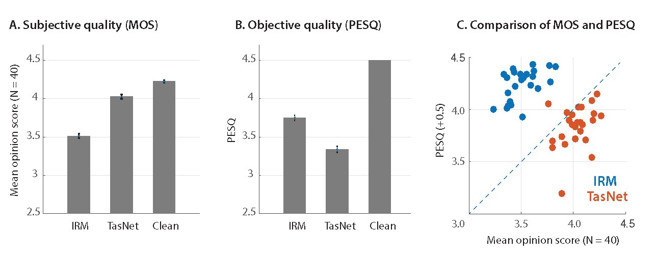
Fig. 3: Subjective and objective quality evaluation of separated utterances in WSJ0-2mix. (A): The mean opinion scores (MOS, N = 40) for IRM, Conv-TasNet and the clean utterance. Conv-TasNet significantly outperforms IRM ($p<1e-16$, t-test). (B): PESQ scores are higher for IRM compared to the Conv-TasNet ($p<1e-16$, t-test). Error bars indicate standard error (STE) (C): MOS versus PESQ for individual utterances. Each dot denotes one mixture utterance, separated using the IRM (blue) or Conv-TasNet (red). The subjective ratings of almost all utterances for Conv-TasNet are higher than their corresponding PESQ scores.

图 3：对 WSJ0-2mix 中分离语句的主观与客观质量评价。（A）IRM、Conv-TasNet 和干净语句的平均意见分（MOS，$N = 40$）。Conv-TasNet 显著优于 IRM（$p<1e-16$，t 检验）。（B）IRM 的 PESQ 分数高于 Conv-TasNet（$p<1e-16$，t 检验）。误差线表示标准误（STE）。（C）各条语句的 MOS 相对 PESQ。每个点表示一条混合语句，分别用 IRM（蓝色）或 Conv-TasNet（红色）分离。Conv-TasNet 几乎所有语句的主观评分都高于它们相应的 PESQ 分数。

IV-E Processing speed comparison

IV-E 处理速度比较

Table VIII compares the processing speed of LSTM-TasNet and causal Conv-TasNet. The speed is evaluated as the average processing time for the systems to separate each frame in the mixtures, which we refer to as time per frame (TPF). TPF determines whether a system can be implemented in real time, which requires a TPF that is smaller than the frame length.

表 VIII 比较了 LSTM-TasNet 与因果 Conv-TasNet 的处理速度。速度按系统分离混合中每一帧所需的平均处理时间来评价，我们称之为每帧时间（TPF）。TPF 决定一个系统能否实时实现，实时要求 TPF 小于帧长。

For the CPU configuration, we tested the system with one processor on an Intel Core i7-5820K CPU. For the GPU configuration, we preloaded both the systems and the data to a Nvidia Titan Xp GPU. LSTM-TasNet with CPU configuration has a TPF close to its frame length (5 ms), which is only marginally acceptable in applications where only a slower CPU is available. Moreover, the processing in LSTM-TasNet is done sequentially, which means that the processing of each time frame must wait for the completion of the previous time frame, further increasing the total processing time of the entire utterance. Since Conv-TasNet decouples the processing of consecutive frames, the processing of subsequent frames does not have to wait until the completion of the current frame and allows the possibility of parallel computing. This process leads to a TPF that is 5 times smaller than the frame length (2 ms) in our CPU configuration. Therefore, even with slower CPUs, Conv-TasNet can still perform real-time separation.

在 CPU 配置下，我们在一颗 Intel Core i7-5820K CPU 上用单个处理器测试系统。在 GPU 配置下，我们把系统和数据都预先加载到一块 Nvidia Titan Xp GPU 上。LSTM-TasNet 在 CPU 配置下的 TPF 接近其帧长（5 毫秒），在只有较慢 CPU 可用的应用中只是勉强可接受。此外，LSTM-TasNet 中的处理是顺序进行的，也就是说每一时间帧的处理必须等上一帧完成，这会进一步增加整句的总处理时间。由于 Conv-TasNet 把相邻帧的处理解耦开来，后续帧不必等到当前帧完成，因而有可能并行计算。在我们的 CPU 配置下，这一过程使 TPF 达到帧长（2 毫秒）的五分之一。因此，即便使用更慢的 CPU，Conv-TasNet 仍然可以做实时分离。

Method	CPU/GPU TPF (ms)
LSTM-TasNet	4.3/0.2
Conv-TasNet-cLN	0.4/0.02

TABLE VIII: Processing time for causal LSTM-TasNet and Conv-TasNet. The speed is evaluated as the average time required to separate a frame (time per frame, TPF).

方法	CPU/GPU TPF（毫秒）
LSTM-TasNet	4.3/0.2
Conv-TasNet-cLN	0.4/0.02

表 VIII：因果 LSTM-TasNet 与 Conv-TasNet 的处理时间。速度按分离一帧所需的平均时间（每帧时间，TPF）评价。

IV-F Sensitivity of LSTM-TasNet to the mixture starting point

IV-F LSTM-TasNet 对混合起点的敏感性

Unlike language processing tasks where sentences have determined starting words, it is difficult to define a general starting sample or frame for speech separation and enhancement tasks. A robust audio processing system should therefore be insensitive to the starting point of the mixture. However, we empirically found that the performance of the causal LSTM-TasNet is very sensitive to the exact starting point of the mixture, which means that shifting the input mixture by several samples may adversely affect the separation accuracy. We systematically examined the robustness of LSTM-TasNet and causal Conv-TasNet to the starting point of the mixture by evaluating the separation accuracy for each mixture in the WSJ0-2mix test set with different sample shifts of the input. A shift of $s$ samples corresponds to starting the separation at sample $s$ instead of the first sample. Figure 4 (A) shows the performance of both systems on the same example mixture with different values of input shift. We observe that, unlike LSTM-TasNet, the causal Conv-TasNet performs consistently well for all shift values of the input mixture. We further tested the overall robustness for the entire test set by calculating the standard deviation of SDRi in each mixture with shifted mixture inputs similar to figure 4 (A). The box plots of all the mixtures in the WSJ0-2mix test set in figure 4 (B) show that causal Conv-TasNet performs consistently better across the entire test set, which confirms the robustness of Conv-TasNet to variations in the starting point of the mixture. One explanation for this inconsistency may be due to the sequential processing constraint in LSTM-TasNet which means that failures in previous frames can accumulate and affect the separation performance in all following frames, while the decoupled processing of consecutive frames in Conv-TasNet alleviates the effect of occasional error.

与句子有确定起始词的语言处理任务不同，语音分离和增强任务很难定义一个通用的起始样本或起始帧。因此，稳健的音频处理系统应当对混合信号的起点不敏感。不过，我们从经验上发现，因果 LSTM-TasNet 的表现对混合信号的精确起点非常敏感，也就是说，把输入混合平移几个样本，就可能对分离精度产生不利影响。我们通过在 WSJ0-2mix 测试集的每条混合上、用不同的输入样本平移评估分离精度，系统地考察了 LSTM-TasNet 和因果 Conv-TasNet 对混合起点的稳健性。平移 $s$ 个样本，对应的是从第 $s$ 个样本而不是从第一个样本开始分离。图 4（A）给出了两个系统在同一条示例混合上、随输入平移取值不同的表现。我们看到，与 LSTM-TasNet 不同，因果 Conv-TasNet 对输入混合的所有平移取值都表现稳定。我们还用与图 4（A）类似的方式，计算每条混合在输入平移下 SDRi 的标准差，以检验整个测试集上的总体稳健性。图 4（B）中 WSJ0-2mix 测试集全部混合的箱线图表明，因果 Conv-TasNet 在整个测试集上都更稳定，这确认了 Conv-TasNet 对混合起点变化的稳健性。一种解释是：LSTM-TasNet 具有顺序处理约束，先前帧的失败会累积并影响后续所有帧的分离表现，而 Conv-TasNet 对相邻帧的解耦处理减轻了偶发错误的影响。

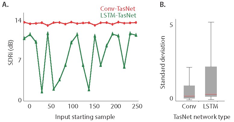
Fig. 4: (A): SDRi of an example mixture separated using LSTM-TasNet and causal Conv-TasNet as a function of the starting point in the mixture. The performance of Conv-TasNet is considerably more consistent and insensitive to the start point. (B): Standard deviation of SDRi across all the mixtures in the WSJ0-2mix test set with varying starting points.

图 4：（A）用 LSTM-TasNet 和因果 Conv-TasNet 分离一条示例混合时，SDRi 随混合中起点的变化。Conv-TasNet 的表现明显更加稳定，对起点不敏感。（B）在起点变化的情况下，WSJ0-2mix 测试集全部混合上 SDRi 的标准差。

IV-G Properties of the basis functions

IV-G 基函数的性质

One of the motivations for replacing the STFT representation of the mixture signal with the convolutional encoder in TasNet was to construct a representation of the audio that is optimized for speech separation. To shed light on the properties of the encoder and decoder representations, we examine the basis functions of the encoder and decoder (rows of the matrices $\bm{\mathrm{U}}$ and $\bm{\mathrm{V}}$). The basis functions are shown in figure 5 for the best noncausal Conv-TasNet, sorted in the same way as figure 2. The magnitudes of the FFTs for each filter are also shown in the same order. As seen in the figure, the majority of the filters are tuned to lower frequencies. In addition, it shows that filters with the same frequency tuning express various phase values for that frequency. This observation can be seen by the circular shift of the low-frequency basis functions. This result suggests an important role for low-frequency features of speech such as pitch as well as explicit encoding of the phase information to achieve superior speech separation performance.

用卷积编码器替换混合信号的 STFT 表示，动机之一是构造对语音分离加以优化的音频表示。为了说明编码器和解码器表示的性质，我们考察编码器和解码器的基函数（矩阵 $\bm{\mathrm{U}}$ 和 $\bm{\mathrm{V}}$ 的行）。图 5 给出了最好的非因果 Conv-TasNet 的基函数，排序方式与图 2 相同。各滤波器 FFT 的幅度也按同一顺序给出。如图所示，大多数滤波器调谐在较低频率。此外还可以看到，具有相同频率调谐的滤波器对该频率表达了不同的相位取值。这一点可以从低频基函数的循环移位看出来。这一结果提示：语音的低频特征（例如音高）以及相位信息的显式编码，对取得更好的语音分离表现有重要作用。

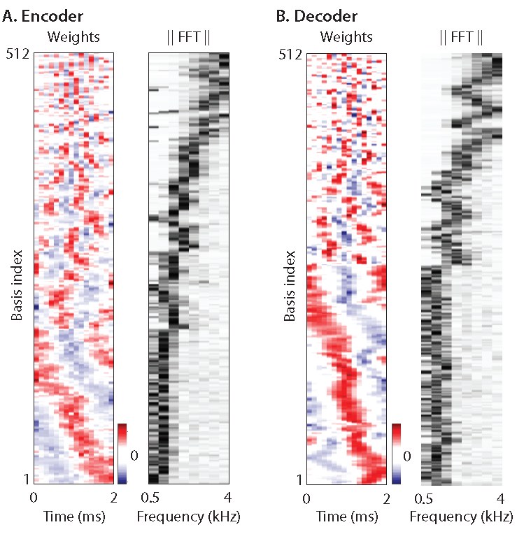
Fig. 5: Visualization of encoder and decoder basis functions and the magnitudes of their FFTs. The basis functions are sorted based on their pairwise Euclidean similarity.

图 5：编码器与解码器基函数及其 FFT 幅度的可视化。基函数按两两欧氏相似度排序。

V Discussion

V 讨论

In this paper, we introduced the fully-convolutional time-domain audio separation network (Conv-TasNet), a deep learning framework for time-domain speech separation. This framework addresses the shortcomings of speech separation in the STFT domain, including the decoupling of phase and magnitude, the suboptimal representation of the mixture audio for separation, and the high latency of calculating the STFT. The improvements are accomplished by replacing the STFT with a convolutional encoder-decoder architecture. The separation in Conv-TasNet is done using a temporal convolutional network (TCN) architecture together with a depthwise separable convolution operation to address the challenges of deep LSTM networks. Our evaluations showed that Conv-TasNet significantly outperforms STFT speech separation systems even when the ideal time-frequency masks for the target speakers are used. In addition, Conv-TasNet has a smaller model size and a shorter minimum latency, which makes it suitable for low-resource, low latency applications.

本文介绍了全卷积时域音频分离网络（Conv-TasNet），这是一套用于时域语音分离的深度学习框架。该框架针对 STFT 域语音分离的几处不足，包括相位与幅度被拆开、混合音频的表示对分离未必最优、以及计算 STFT 的高延迟。改进是通过用卷积编码器–解码器结构替换 STFT 实现的。Conv-TasNet 中的分离采用时间卷积网络（TCN）结构，并配合深度可分离卷积运算，以应对深层 LSTM 网络带来的困难。我们的评价表明，即便与目标说话人的理想时频掩蔽相比，Conv-TasNet 也显著优于基于 STFT 的语音分离系统。此外，Conv-TasNet 的模型更小、最短延迟更短，因而适合低资源、低延迟的应用。

Unlike STFT which has a well-defined inverse transform that can perfectly reconstruct the input, best performance in the proposed model is achieved by an overcomplete linear convolutional encoder-decoder framework without guaranteeing the perfect reconstruction of the input. This observation motivates rethinking of autoencoder and overcompleteness in the source separation problem which may share similarities to the studies of overcomplete dictionary and sparse coding [51, 52]. Moreover, the analysis of the encoder/decoder basis functions in section IV-G revealed two interesting properties. First, most of the filters are tuned to low acoustic frequencies (more than 60% tuned to frequencies below 1 kHz). This pattern of frequency representation, which we found using a data-driven method, roughly resembles the well-known mel-frequency scale [53] as well as the tonotopic organization of the frequencies in the mammalian auditory system [54, 55]. In addition, the overexpression of lower frequencies may indicate the importance of accurate pitch tracking in speech separation, similar to what has been reported in human multitalker perception studies [56]. In addition, we found that filters with the same frequency tuning explicitly express various phase information. In contrast, this information is implicit in the STFT operations, where the real and imaginary parts only represent symmetric (cosine) and asymmetric (sine) phases, respectively. This explicit encoding of signal phase values may be the key reason for the superior performance of TasNet over the STFT-based separation methods.

STFT 有定义明确、可以完美重建输入的逆变换；而在所提出的模型中，最好的表现来自过完备的线性卷积编码器–解码器框架，并不保证输入被完美重建。这一观察促使我们重新思考源分离问题中的自编码器与过完备性，它可能与过完备字典和稀疏编码方面的研究有相似之处 [51, 52]。此外，第 IV-G 节对编码器/解码器基函数的分析揭示了两个有意思的性质。第一，大多数滤波器调谐在较低的声学频率上（超过 60% 调谐在 1 kHz 以下）。我们用数据驱动方法得到的这一频率表示模式，大致类似于为人熟知的梅尔频率尺度 [53]，也类似于哺乳动物听觉系统中频率的音调拓扑组织 [54, 55]。此外，对较低频率的过度表达，可能表明准确的音高跟踪在语音分离中很重要，这与人类多说话人感知研究中的报告相似 [56]。另外，我们发现具有相同频率调谐的滤波器会显式表达不同的相位信息。相比之下，这一信息在 STFT 运算中是隐含的：实部和虚部分别只表示对称（余弦）和反对称（正弦）相位。对信号相位取值的这种显式编码，可能是 TasNet 优于基于 STFT 的分离方法的关键原因。

The combination of high accuracy, short latency, and small model size makes Conv-TasNet a suitable choice for both offline and real-time, low-latency speech processing applications such as embedded systems and wearable hearing and telecommunication devices. Conv-TasNet can also serve as a front-end module for tandem systems in other audio processing tasks, such as multitalker speech recognition [57, 58, 59, 60] and speaker identification [61, 62]. On the other hand, several limitations of Conv-TasNet must be addressed before it can be actualized, including the long-term tracking of speakers and generalization to noisy and reverberant environments. Because Conv-TasNet uses a fixed temporal context length, the long-term tracking of an individual speaker may fail, particularly when there is a long pause in the mixture audio. In addition, the generalization of Conv-TasNet to noisy and reverberant conditions must be further tested [26], as time-domain approaches are more prone to temporal distortions which are particularly severe in reverberant acoustic environments. In such conditions, extending the Conv-TasNet framework to incorporate multiple input audio channels may prove advantageous when more than one microphone is available. Previous studies have shown the benefit of extending speech separation to multichannel inputs [63, 64, 65], particularly in adverse acoustic conditions and when the number of interfering speakers is large (e.g., more than 3).

高精度、短延迟和小模型规模结合在一起，使 Conv-TasNet 既适合离线，也适合实时、低延迟的语音处理应用，例如嵌入式系统以及可穿戴助听和通信设备。Conv-TasNet 也可以作为前端模块，用于其他音频处理任务中的串联系统，例如多说话人语音识别 [57, 58, 59, 60] 和说话人辨认 [61, 62]。另一方面，Conv-TasNet 仍有若干限制需要解决，才能真正落地，包括对说话人的长期跟踪，以及向含噪和混响环境的泛化。由于 Conv-TasNet 使用固定的时间上下文长度，对单个说话人的长期跟踪可能会失败，尤其是当混合音频中出现较长停顿时。此外，Conv-TasNet 在含噪和混响条件下的泛化还需要进一步检验 [26]，因为时域方法更容易受到时间失真的影响，而这类失真在混响声学环境中尤为严重。在这类条件下，若有不止一只麦克风可用，把 Conv-TasNet 框架扩展到多通道输入音频可能会有帮助。以往研究已经表明，把语音分离扩展到多通道输入是有益的 [63, 64, 65]，尤其是在不利声学条件以及干扰说话人较多（例如多于 3 个）时。

In summary, Conv-TasNet represents a significant step toward the realization of speech separation algorithms and opens many future research directions that would further improve its accuracy, speed, and computational cost, which could eventually make automatic speech separation a common and necessary feature of every speech processing technology designed for real-world applications.

总的来说，Conv-TasNet 朝着实现语音分离算法迈出了重要一步，并打开了许多未来研究方向，以进一步改善其精度、速度和计算代价，最终有可能使自动语音分离成为每一项面向真实世界应用的语音处理技术中常见而必要的功能。

VI Acknowledgments

VI 致谢

This work was funded by a grant from the National Institute of Health, NIDCD, DC014279; a National Science Foundation CAREER Award; and the Pew Charitable Trusts.

本工作得到美国国立卫生研究院 NIDCD 资助 DC014279、美国国家科学基金会 CAREER Award，以及皮尤慈善信托基金的资助。

Notes

注释

[^1] With our Pytorch implementation, this is possibly due to the different autograd mechanisms in fully-connected layer and 1-D (transposed) convolutional layers.

[^1] 在我们的 Pytorch 实现中，这可能是因为全连接层与一维（转置）卷积层的 autograd 机制不同。

[^2] https://github.com/naplab/Conv-TasNet

References

参考文献

[1] D. Wang and J. Chen, “Supervised speech separation based on deep learning: An overview,” IEEE/ACM Transactions on Audio, Speech, and Language Processing , 2018.

[2] X. Lu, Y. Tsao, S. Matsuda, and C. Hori, “Speech enhancement based on deep denoising autoencoder.” in Interspeech , 2013, pp. 436–440.

[3] Y. Xu, J. Du, L.-R. Dai, and C.-H. Lee, “An experimental study on speech enhancement based on deep neural networks,” IEEE Signal processing letters , vol. 21, no. 1, pp. 65–68, 2014.

[4] ——, “A regression approach to speech enhancement based on deep neural networks,” IEEE/ACM Transactions on Audio, Speech and Language Processing (TASLP) , vol. 23, no. 1, pp. 7–19, 2015.

[5] Y. Isik, J. Le Roux, Z. Chen, S. Watanabe, and J. R. Hershey, “Single-channel multi-speaker separation using deep clustering,” Interspeech 2016 , pp. 545–549, 2016.

[6] D. Yu, M. Kolbæk, Z.-H. Tan, and J. Jensen, “Permutation invariant training of deep models for speaker-independent multi-talker speech separation,” in Acoustics, Speech and Signal Processing (ICASSP), 2017 IEEE International Conference on . IEEE, 2017, pp. 241–245.

[7] M. Kolbæk, D. Yu, Z.-H. Tan, and J. Jensen, “Multitalker speech separation with utterance-level permutation invariant training of deep recurrent neural networks,” IEEE/ACM Transactions on Audio, Speech, and Language Processing , vol. 25, no. 10, pp. 1901–1913, 2017.

[8] Z. Chen, Y. Luo, and N. Mesgarani, “Deep attractor network for single-microphone speaker separation,” in Acoustics, Speech and Signal Processing (ICASSP), 2017 IEEE International Conference on . IEEE, 2017, pp. 246–250.

[9] Y. Luo, Z. Chen, and N. Mesgarani, “Speaker-independent speech separation with deep attractor network,” IEEE/ACM Transactions on Audio, Speech, and Language Processing , vol. 26, no. 4, pp. 787–796, 2018. [Online]. Available: http://dx.doi.org/10.1109/TASLP.2018.2795749

[10] Z.-Q. Wang, J. Le Roux, and J. R. Hershey, “Alternative objective functions for deep clustering,” in Proc. IEEE International Conference on Acoustics, Speech and Signal Processing (ICASSP) , 2018.

[11] Z.-Q. Wang, J. L. Roux, D. Wang, and J. R. Hershey, “End-to-end speech separation with unfolded iterative phase reconstruction,” arXiv preprint arXiv:1804.10204 , 2018.

[12] C. Li, L. Zhu, S. Xu, P. Gao, and B. Xu, “ CBLDNN -based speaker-independent speech separation via generative adversarial training,” in Acoustics, Speech and Signal Processing (ICASSP), 2018 IEEE International Conference on . IEEE, 2018.

[13] D. Griffin and J. Lim, “Signal estimation from modified short-time fourier transform,” IEEE Transactions on Acoustics, Speech, and Signal Processing , vol. 32, no. 2, pp. 236–243, 1984.

[14] J. Le Roux, N. Ono, and S. Sagayama, “Explicit consistency constraints for stft spectrograms and their application to phase reconstruction.” in SAPA@ INTERSPEECH , 2008, pp. 23–28.

[15] Y. Luo, Z. Chen, J. R. Hershey, J. Le Roux, and N. Mesgarani, “Deep clustering and conventional networks for music separation: Stronger together,” in Acoustics, Speech and Signal Processing (ICASSP), 2017 IEEE International Conference on . IEEE, 2017, pp. 61–65.

[16] A. Jansson, E. Humphrey, N. Montecchio, R. Bittner, A. Kumar, and T. Weyde, “Singing voice separation with deep u-net convolutional networks,” in 18th International Society for Music Information Retrieval Conference , 2017, pp. 23–27.

[17] S. Choi, A. Cichocki, H.-M. Park, and S.-Y. Lee, “Blind source separation and independent component analysis: A review,” Neural Information Processing-Letters and Reviews , vol. 6, no. 1, pp. 1–57, 2005.

[18] K. Yoshii, R. Tomioka, D. Mochihashi, and M. Goto, “Beyond nmf: Time-domain audio source separation without phase reconstruction.” in ISMIR , 2013, pp. 369–374.

[19] S. Venkataramani, J. Casebeer, and P. Smaragdis, “End-to-end source separation with adaptive front-ends,” arXiv preprint arXiv:1705.02514 , 2017.

[20] D. Stoller, S. Ewert, and S. Dixon, “Wave-u-net: A multi-scale neural network for end-to-end audio source separation,” arXiv preprint arXiv:1806.03185 , 2018.

[21] Y. Luo and N. Mesgarani, “Tasnet: time-domain audio separation network for real-time, single-channel speech separation,” in Acoustics, Speech and Signal Processing (ICASSP), 2018 IEEE International Conference on . IEEE, 2018.

[22] S.-W. Fu, T.-W. Wang, Y. Tsao, X. Lu, and H. Kawai, “End-to-end waveform utterance enhancement for direct evaluation metrics optimization by fully convolutional neural networks,” IEEE/ACM Transactions on Audio, Speech and Language Processing (TASLP) , vol. 26, no. 9, pp. 1570–1584, 2018.

[23] S. Pascual, A. Bonafonte, and J. Serrà, “Segan: Speech enhancement generative adversarial network,” Proc. Interspeech 2017 , pp. 3642–3646, 2017.

[24] O. Ronneberger, P. Fischer, and T. Brox, “U-net: Convolutional networks for biomedical image segmentation,” in International Conference on Medical image computing and computer-assisted intervention . Springer, 2015, pp. 234–241.

[25] J. R. Hershey, Z. Chen, J. Le Roux, and S. Watanabe, “Deep clustering: Discriminative embeddings for segmentation and separation,” in Acoustics, Speech and Signal Processing (ICASSP), 2016 IEEE International Conference on . IEEE, 2016, pp. 31–35.

[26] Y. Luo and N. Mesgarani, “Real-time single-channel dereverberation and separation with time-domain audio separation network,” Proc. Interspeech 2018 , pp. 342–346, 2018.

[27] F.-Y. Wang, C.-Y. Chi, T.-H. Chan, and Y. Wang, “Nonnegative least-correlated component analysis for separation of dependent sources by volume maximization,” IEEE transactions on pattern analysis and machine intelligence , vol. 32, no. 5, pp. 875–888, 2010.

[28] C. H. Ding, T. Li, and M. I. Jordan, “Convex and semi-nonnegative matrix factorizations,” IEEE transactions on pattern analysis and machine intelligence , vol. 32, no. 1, pp. 45–55, 2010.

[29] C. Lea, R. Vidal, A. Reiter, and G. D. Hager, “Temporal convolutional networks: A unified approach to action segmentation,” in European Conference on Computer Vision . Springer, 2016, pp. 47–54.

[30] C. Lea, M. D. Flynn, R. Vidal, A. Reiter, and G. D. Hager, “Temporal convolutional networks for action segmentation and detection,” in proceedings of the IEEE Conference on Computer Vision and Pattern Recognition , 2017, pp. 156–165.

[31] S. Bai, J. Z. Kolter, and V. Koltun, “An empirical evaluation of generic convolutional and recurrent networks for sequence modeling,” arXiv preprint arXiv:1803.01271 , 2018.

[32] F. Chollet, “Xception: Deep learning with depthwise separable convolutions,” arXiv preprint , 2016.

[33] A. G. Howard, M. Zhu, B. Chen, D. Kalenichenko, W. Wang, T. Weyand, M. Andreetto, and H. Adam, “Mobilenets: Efficient convolutional neural networks for mobile vision applications,” arXiv preprint arXiv:1704.04861 , 2017.

[34] D. Wang, “On ideal binary mask as the computational goal of auditory scene analysis,” in Speech separation by humans and machines . Springer, 2005, pp. 181–197.

[35] Y. Li and D. Wang, “On the optimality of ideal binary time–frequency masks,” Speech Communication , vol. 51, no. 3, pp. 230–239, 2009.

[36] Y. Wang, A. Narayanan, and D. Wang, “On training targets for supervised speech separation,” IEEE/ACM Transactions on Audio, Speech and Language Processing (TASLP) , vol. 22, no. 12, pp. 1849–1858, 2014.

[37] H. Erdogan, J. R. Hershey, S. Watanabe, and J. Le Roux, “Phase-sensitive and recognition-boosted speech separation using deep recurrent neural networks,” in Acoustics, Speech and Signal Processing (ICASSP), 2015 IEEE International Conference on . IEEE, 2015, pp. 708–712.

[38] A. Van Den Oord, S. Dieleman, H. Zen, K. Simonyan, O. Vinyals, A. Graves, N. Kalchbrenner, A. Senior, and K. Kavukcuoglu, “Wavenet: A generative model for raw audio,” CoRR abs/1609.03499 , 2016.

[39] L. Kaiser, A. N. Gomez, and F. Chollet, “Depthwise separable convolutions for neural machine translation,” arXiv preprint arXiv:1706.03059 , 2017.

[40] K. He, X. Zhang, S. Ren, and J. Sun, “Delving deep into rectifiers: Surpassing human-level performance on imagenet classification,” in Proceedings of the IEEE international conference on computer vision , 2015, pp. 1026–1034.

[41] J. L. Ba, J. R. Kiros, and G. E. Hinton, “Layer normalization,” arXiv preprint arXiv:1607.06450 , 2016.

[42] “Script to generate the multi-speaker dataset using wsj0,” http://www.merl.com/demos/deep-clustering .

[43] D. Kingma and J. Ba, “Adam: A method for stochastic optimization,” arXiv preprint arXiv:1412.6980 , 2014.

[44] E. Vincent, R. Gribonval, and C. Févotte, “Performance measurement in blind audio source separation,” IEEE transactions on audio, speech, and language processing , vol. 14, no. 4, pp. 1462–1469, 2006.

[45] A. W. Rix, J. G. Beerends, M. P. Hollier, and A. P. Hekstra, “Perceptual evaluation of speech quality (pesq)-a new method for speech quality assessment of telephone networks and codecs,” in Acoustics, Speech, and Signal Processing, 2001. Proceedings.(ICASSP’01). 2001 IEEE International Conference on , vol. 2. IEEE, 2001, pp. 749–752.

[46] ITU-T Rec. P.10, “Vocabulary for performance and quality of service,” 2006.

[47] R. R. Sokal, “A statistical method for evaluating systematic relationship,” University of Kansas science bulletin , vol. 28, pp. 1409–1438, 1958.

[48] M. Sandler, A. Howard, M. Zhu, A. Zhmoginov, and L.-C. Chen, “Mobilenetv2: Inverted residuals and linear bottlenecks,” in Proceedings of the IEEE Conference on Computer Vision and Pattern Recognition , 2018, pp. 4510–4520.

[49] “Audio samples for Conv-TasNet,” http://naplab.ee.columbia.edu/tasnet.html .

[50] C. Xu, X. Xiao, and H. Li, “Single channel speech separation with constrained utterance level permutation invariant training using grid lstm,” in Acoustics, Speech and Signal Processing (ICASSP), 2018 IEEE International Conference on . IEEE, 2018.

[51] T.-W. Lee, M. S. Lewicki, M. Girolami, and T. J. Sejnowski, “Blind source separation of more sources than mixtures using overcomplete representations,” IEEE signal processing letters , vol. 6, no. 4, pp. 87–90, 1999.

[52] M. Zibulevsky and B. A. Pearlmutter, “Blind source separation by sparse decomposition in a signal dictionary,” Neural computation , vol. 13, no. 4, pp. 863–882, 2001.

[53] S. Imai, “Cepstral analysis synthesis on the mel frequency scale,” in Acoustics, Speech, and Signal Processing, IEEE International Conference on ICASSP’83. , vol. 8. IEEE, 1983, pp. 93–96.

[54] G. L. Romani, S. J. Williamson, and L. Kaufman, “Tonotopic organization of the human auditory cortex,” Science , vol. 216, no. 4552, pp. 1339–1340, 1982.

[55] C. Pantev, M. Hoke, B. Lutkenhoner, and K. Lehnertz, “Tonotopic organization of the auditory cortex: pitch versus frequency representation,” Science , vol. 246, no. 4929, pp. 486–488, 1989.

[56] C. J. Darwin, D. S. Brungart, and B. D. Simpson, “Effects of fundamental frequency and vocal-tract length changes on attention to one of two simultaneous talkers,” The Journal of the Acoustical Society of America , vol. 114, no. 5, pp. 2913–2922, 2003.

[57] J. R. Hershey, S. J. Rennie, P. A. Olsen, and T. T. Kristjansson, “Super-human multi-talker speech recognition: A graphical modeling approach,” Computer Speech & Language , vol. 24, no. 1, pp. 45–66, 2010.

[58] C. Weng, D. Yu, M. L. Seltzer, and J. Droppo, “Deep neural networks for single-channel multi-talker speech recognition,” IEEE/ACM Transactions on Audio, Speech and Language Processing (TASLP) , vol. 23, no. 10, pp. 1670–1679, 2015.

[59] Y. Qian, X. Chang, and D. Yu, “Single-channel multi-talker speech recognition with permutation invariant training,” arXiv preprint arXiv:1707.06527 , 2017.

[60] K. Ochi, N. Ono, S. Miyabe, and S. Makino, “Multi-talker speech recognition based on blind source separation with ad hoc microphone array using smartphones and cloud storage.” in INTERSPEECH , 2016, pp. 3369–3373.

[61] Y. Lei, N. Scheffer, L. Ferrer, and M. McLaren, “A novel scheme for speaker recognition using a phonetically-aware deep neural network,” in Acoustics, Speech and Signal Processing (ICASSP), 2014 IEEE International Conference on . IEEE, 2014, pp. 1695–1699.

[62] M. McLaren, Y. Lei, and L. Ferrer, “Advances in deep neural network approaches to speaker recognition,” in Acoustics, Speech and Signal Processing (ICASSP), 2015 IEEE International Conference on . IEEE, 2015, pp. 4814–4818.

[63] S. Gannot, E. Vincent, S. Markovich-Golan, A. Ozerov, S. Gannot, E. Vincent, S. Markovich-Golan, and A. Ozerov, “A consolidated perspective on multimicrophone speech enhancement and source separation,” IEEE/ACM Transactions on Audio, Speech and Language Processing (TASLP) , vol. 25, no. 4, pp. 692–730, 2017.

[64] Z. Chen, J. Li, X. Xiao, T. Yoshioka, H. Wang, Z. Wang, and Y. Gong, “Cracking the cocktail party problem by multi-beam deep attractor network,” in Automatic Speech Recognition and Understanding Workshop (ASRU), 2017 IEEE . IEEE, 2017, pp. 437–444.

[65] Z.-Q. Wang, J. Le Roux, and J. R. Hershey, “Multi-channel deep clustering: Discriminative spectral and spatial embeddings for speaker-independent speech separation,” in Acoustics, Speech and Signal Processing (ICASSP), 2018 IEEE International Conference on . IEEE, 2018.