Conformal Prediction as Bayesian Quadrature

Conformal Prediction as Bayesian Quadrature：将共形预测视为贝叶斯求积

Jake C. Snell Affiliation:  Department of Computer Science, Princeton University Correspondence to: jsnell@princeton.edu    Thomas L. Griffiths Affiliation:  Department of Psychology, Princeton University Affiliation:  Department of Computer Science, Princeton University

Abstract

摘要

As machine learning-based prediction systems are increasingly used in high-stakes situations, it is important to understand how such predictive models will perform upon deployment. Distribution-free uncertainty quantification techniques such as conformal prediction provide guarantees about the loss black-box models will incur even when the details of the models are hidden. However, such methods are based on frequentist probability, which unduly limits their applicability. We revisit the central aspects of conformal prediction from a Bayesian perspective and thereby illuminate the shortcomings of frequentist guarantees. We propose a practical alternative based on Bayesian quadrature that provides interpretable guarantees and offers a richer representation of the likely range of losses to be observed at test time.

随着基于机器学习的预测系统越来越多用于高风险场景，有必要理解这类预测模型在部署后的表现。共形预测等分布无关不确定性量化技术，即便模型细节不可见，也能对黑盒模型将承受的损失给出保证。然而这些方法建立在频率派概率之上，适用范围被不必要地收窄。我们从贝叶斯视角重审共形预测的核心环节，从而澄清频率派保证的不足。我们提出一种基于贝叶斯求积的实用替代：提供可解释的保证，并更丰富地刻画测试时可能观察到的损失范围。

1 Introduction

1 引言

Keywords:

Machine learning systems based on deep learning are increasingly used in high-stakes settings, such as medical diagnosis or financial applications. These settings impose unique constraints on the performance of these systems: we want them to produce good outcomes in the aggregate, but also do so fairly and with a guarantee of a low probability of harm. However, predictive models based on deep learning can be difficult to interpret, and commercial models increasingly tend to offer little information about the techniques used in training. This creates a new challenge: How can we flexibly and reliably quantify the suitability of a model for deployment without making too many assumptions about how the model was trained or in which settings it will be used?

关键词：

基于深度学习的机器学习系统正越来越多用于医疗诊断、金融应用等高风险设定。这些设定对系统表现施加独特约束：我们既希望总体结果良好，也希望公平，并对低伤害概率给出保证。但深度学习预测模型往往难以解释，商业模型也越来越少披露训练细节。这就提出新挑战：在不过多假设模型如何训练、将用于何种场景的前提下，如何灵活且可靠地量化模型是否适合部署？

Recent research on quantifying uncertainty has employed methods based on conformal prediction (Vovk et al., 2005), which aim to provide guarantees for model performance in a distribution-free way. However, these techniques are based on ideas from frequentist statistics, making it difficult to incorporate prior knowledge that might be available about specific models. For example, in a particular setting we might have access to some information about the distribution of the data that is likely to be encountered, and can construct tighter guarantees on the performance of models by making use of this information. Moreover, they focus on controlling the expected loss averaged over many unobserved datasets rather than focusing on the actual set of observations.

近期不确定性量化研究采用共形预测（Vovk 等，2005）等方法，试图以分布无关方式给出模型表现保证。但这些技术基于频率派统计思想，难以融入关于特定模型的先验知识。例如，在某设定下我们可能对将遇到的数据分布有部分信息，利用这些信息可构造更紧的模型表现保证。此外，它们关注的是对许多未观测数据集平均的期望损失，而非实际观测集合本身。

In this paper, we show how methods for guaranteeing model performance can be understood and extended by viewing them from a Bayesian perspective. We develop a framework in which we explicitly model uncertainty in the quantile values associated with particular observations, providing a nonparametric tool for characterizing possible distributions where the model might be deployed that is appropriately constrained by observed data. This framework allows us to draw upon methods from the fields of statistical prediction analysis (Aitchison & Dunsmore, 1975) and probabilistic numerics (Cockayne et al., 2019; Hennig et al., 2022) to develop guarantees that are interpretable and make adaptive use of available information.

本文表明，从贝叶斯视角理解并扩展保证模型表现的方法是可行的。我们建立一个框架，显式建模与特定观测相关的分位数值不确定性，提供受观测数据恰当约束的非参数工具，用以刻画模型可能部署的分布。该框架让我们借用统计预测分析（Aitchison & Dunsmore，1975）与概率数值（Cockayne 等，2019；Hennig 等，2022）的方法，发展可解释、并能自适应利用可用信息的保证。

We show that two popular uncertainty quantification methods, split conformal prediction (Vovk et al., 2005; Papadopoulos et al., 2002) and conformal risk control (Angelopoulos et al., 2024), can both be recovered as special cases of our framework. Our approach gives a more complete characterization of the performance of these approaches, as we are able to determine the full distribution of possible outcomes rather than a single point estimate. Since our approach is grounded in Bayesian probability, we can easily incorporate knowledge relevant to evaluating the performance of these models when it is present, such as monotonicity or distributional assumptions, while defaulting to existing methods when absent. Our results show that Bayesian probability, while it is often discarded due to the apparent need to specify prior distributions, is actually well-suited for distribution-free uncertainty quantification.

我们证明两种流行的不确定性量化方法——分割共形预测（Vovk 等，2005；Papadopoulos 等，2002）与共形风险控制（Angelopoulos 等，2024）——都可作为本框架的特例恢复。由于能给出可能结果的完整分布而非单一点估计，我们对这些方法的表现刻画更完整。方法植根于贝叶斯概率，因此在相关知识存在时易于融入（如单调性或分布假设），缺失时则回退到既有方法。结果表明：贝叶斯概率常因「似乎必须指定先验」而被搁置，实际上却很适合分布无关不确定性量化。

2 Background

2 背景

Conformal prediction methods apply a wrapper on top of black-box predictive models to be able to subject them to statistical analysis. In order to generate meaningful predictions about future performance, it is assumed that we have access to a small calibration dataset that is representative of the deployment conditions. Performance on this dataset then provides the foundation for generating predictions about future performance. We begin by reviewing existing current distribution-free uncertainty quantification techniques and Bayesian quadrature methods.

共形预测方法在黑盒预测模型外包一层包装，以便对其做统计分析。为对未来表现做出有意义的预测，假定我们拥有一小份能代表部署条件的校准数据集；该集上的表现再作为推断未来表现的基础。我们先回顾现有分布无关不确定性量化技术与贝叶斯求积方法。

2.1 Distribution-free Uncertainty Quantification Techniques

2.1 分布无关不确定性量化技术

Uncertainty quantification techniques provide guarantees on the future performance of a black-box predictive model mapping inputs $X$ to outputs $Y$ based on a calibration set consisting of $X_{1},\ldots,X_{n}$ and $Y_{1},\ldots,Y_{n}$. Different approaches do so in different ways. For more information on these techniques, refer to Shafer & Vovk (2008) or Angelopoulos & Bates (2023).

不确定性量化技术基于由 $X_{1},\ldots,X_{n}$ 与 $Y_{1},\ldots,Y_{n}$ 组成的校准集，对把输入 $X$ 映到输出 $Y$ 的黑盒预测模型给出未来表现保证。不同方法路径不同。更多介绍见 Shafer & Vovk（2008）或 Angelopoulos & Bates（2023）。

Split Conformal Prediction

The goal of Split Conformal Prediction (Vovk et al., 2005; Papadopoulos et al., 2002) is to generate a prediction set or interval that contains the ground-truth output with high probability. This is often expressed in terms of the coverage level $1-\alpha$. It relies on a score function $s(x,y)$ which measures the disagreement between a predictor’s output and the ground truth.

分割共形预测

分割共形预测（Vovk 等，2005；Papadopoulos 等，2002）的目标是生成以高概率包含真值输出的预测集或区间，常写成覆盖水平 $1-\alpha$。它依赖评分函数 $s(x,y)$，度量预测器输出与真值的不一致。

The conformal guarantee is

共形保证为

$$\Pr\left(Y_{n+1}\notin\mathcal{C}(X_{n+1})\right)\leq\alpha, \tag{1}$$

where

其中

$$\mathcal{C}(X_{n+1})=\left\{y:s(X_{n+1},y)\leq\hat{q}\right\} \tag{2}$$

and $\hat{q}$ is the $\frac{\lceil(n+1)(1-\alpha)\rceil}{n}$ quantile of $s_{1}=s(X_{1},Y_{1}),\ldots,s_{n}=s(X_{n},Y_{n})$. Here, $\mathcal{C}(X_{{n+1}})$ is a prediction set or interval which aims to include the ground-truth output.

且 $\hat{q}$ 是 $s_{1}=s(X_{1},Y_{1}),\ldots,s_{n}=s(X_{n},Y_{n})$ 的 $\frac{\lceil(n+1)(1-\alpha)\rceil}{n}$ 分位数。这里 $\mathcal{C}(X_{{n+1}})$ 是旨在包含真值输出的预测集或区间。

Conformal Risk Control

In Conformal Risk Control (Angelopoulos et al., 2024), the goal is to generalize conformal prediction to more general loss functions that are monotonic functions of a single parameter $\lambda$. Conformal Risk Control (CRC) proceeds by viewing the coverage guarantee (1) as the expected value of a 0-1 loss. It is assumed that the maximum possible value of the loss is $B$ and that the problem is “achievable” by design in that there exists some setting $\lambda_{\text{max}}$ that satisfies the conformal guarantee. Additionally, each loss function $L_{i}(\lambda)$ is assumed to be a monotonic non-increasing function of $\lambda$. The guarantee offered by Conformal Risk Control is of the form

共形风险控制

在共形风险控制（Angelopoulos 等，2024）中，目标是把共形预测推广到关于单参数 $\lambda$ 单调的更一般损失函数。共形风险控制（CRC）把覆盖保证（1）视为 0-1 损失的期望。假定损失最大可能值为 $B$，且问题「可达成」——存在某个 $\lambda_{\text{max}}$ 满足共形保证。此外，每个损失函数 $L_{i}(\lambda)$ 假定对 $\lambda$ 单调非增。共形风险控制给出的保证形如

$$E\left(\ell(\mathcal{C}_{\hat{\lambda}}(X_{n+1}),Y_{n+1})\right)\leq\alpha, \tag{3}$$

where

其中

$$\hat{\lambda}=\inf\left\{\lambda:\frac{n}{n+1}\hat{R}_{n}(\lambda)+\frac{B}{n+1}\leq\alpha\right\} \tag{4}$$

and $\hat{R}_{n}(\lambda)=\frac{1}{n}\sum_{i=1}^{n}L_{i}(\lambda)$ is the empirical risk.

且 $\hat{R}_{n}(\lambda)=\frac{1}{n}\sum_{i=1}^{n}L_{i}(\lambda)$ 为经验风险。

2.2 Bayesian Quadrature

2.2 贝叶斯求积

Bayesian quadrature (Diaconis, 1988; O’Hagan, 1991) is a general technique for evaluating integrals that allows for uncertainty in the integrand. It estimates the value of an integral $\int_{a}^{b}f(x)\,dx$ by the following four steps: (1) place a prior $p(f)$ on functions, (2) evaluate $f$ at $x_{1},x_{2},\ldots,x_{n}$, (3) compute a posterior given the observed values of $f$ by Bayes’ rule, and (4) estimate $\int_{a}^{b}f(x)\,dx$. Suppose that $f(x_{i})=y_{i}$ for $i=1,2,\ldots,n$. The posterior over $f$ is

贝叶斯求积（Diaconis，1988；O’Hagan，1991）是一类允许被积函数不确定的积分求值技术。它按四步估计积分 $\int_{a}^{b}f(x)\,dx$：（1）在函数上放先验 $p(f)$；（2）在 $x_{1},x_{2},\ldots,x_{n}$ 处求值 $f$；（3）由观测值经贝叶斯公式算后验；（4）估计 $\int_{a}^{b}f(x)\,dx$。设 $f(x_{i})=y_{i}$（$i=1,2,\ldots,n$），则 $f$ 的后验为

$$p(f\mid x_{1:n},y_{1:n})\propto p(f)\prod_{i=1}^{n}\delta(y_{i}-f(x_{i})), \tag{5}$$

where $\delta(\cdot)$ is the Dirac delta function. The posterior mean then provides an estimate for the integral:

其中 $\delta(\cdot)$ 是 Dirac δ 函数。后验均值随后给出积分估计：

$$\displaystyle\int_{a}^{b}f(x)\,dx \\ \displaystyle\approx\int_{a}^{b}f_{n}(x)\,dx,\text{ where } \\ \displaystyle f_{n}(t) \\ \displaystyle=E(f(t)\mid x_{1:n},y_{1:n}). \tag{6}$$

It has been demonstrated that many classical quadrature procedures such as the trapezoid rule can be recovered by placing a Gaussian process prior on functions (Karvonen & Särkkä, 2017).

已证明，在函数上放置高斯过程先验时，可恢复梯形法则等许多经典求积程序（Karvonen & Särkkä，2017）。

2.3 Summary and Prospectus

2.3 小结与展望

Bayesian quadrature provides an illustration of how a primarily numerical method can be connected to Bayesian inference, and in doing so potentially admit additional information about the underlying function that can be incorporated via a prior distribution. In next section, we will see how a similar approach can be applied to conformal prediction, identifying a Bayesian framework that reproduces existing distribution-free uncertainty quantification techniques. The challenge in doing so is that we want guarantees of the style obtained from Bayesian models, but we want to make the approach as general as possible in its assumptions about the underlying distribution. We solve this problem via an approach inspired by probabilistic numerics to construct a nonparametric characterization of the underlying distribution based on the calibration set.

贝叶斯求积说明：一项以数值为主的方法可以接到贝叶斯推断，并因此允许经先验融入关于底层函数的额外信息。下一节将看到，类似思路可用于共形预测，找出能复现既有分布无关不确定性量化技术的贝叶斯框架。难点在于：我们既想要贝叶斯模型式的保证风格，又希望对底层分布的假设尽可能一般。我们借鉴概率数值，基于校准集构造底层分布的非参数刻画，从而解决这一问题。

3 Decision-theoretic Formulation

3 决策论表述

In this section we show how split conformal prediction and conformal risk control can be formulated as instances of a general decision problem.

本节说明如何把分割共形预测与共形风险控制表述为一般决策问题的实例。

Let $z=(z_{1},\ldots,z_{n})$ be a set of calibration data where each observation $z_{i}=(x_{i},y_{i})$ consists of an input and a ground truth label. Let $\theta$ denote the true state of nature that defines a shared density $f(z_{i}\mid\theta)$ for the data.[^1] A new test point $z_{\text{new}}$ is assumed to have the same distribution. Let $\lambda$ be a control parameter (e.g. threshold) that must be chosen based on the calibration data. We assume the presence of a loss function $L(\theta,\lambda)$ which quantifies the loss incurred by selecting $\lambda$ when the true state of nature is $\theta$.

设 $z=(z_{1},\ldots,z_{n})$ 为校准数据，每个观测 $z_{i}=(x_{i},y_{i})$ 由输入与真值标签组成。令 $\theta$ 表示定义数据共享密度 $f(z_{i}\mid\theta)$ 的真实自然状态。[1] 新测试点 $z_{\text{new}}$ 假定服从同一分布。令 $\lambda$ 为必须基于校准数据选择的控制参数（例如阈值）。我们假定存在损失函数 $L(\theta,\lambda)$，量化在真实状态为 $\theta$ 时选择 $\lambda$ 所招致的损失。

The decision-theoretic goal is to choose a decision rule $\lambda(z)$ that controls the risk:

决策论目标是选择控制风险的决策规则 $\lambda(z)$：

$$R(\theta,\lambda)=\int L(\theta,\lambda(z))f(z\mid\theta)\,dz. \tag{8}$$

It is often desirable to choose $\lambda$ so that it is robust to any possible state of nature $\theta$. The maximum risk is defined as

往往希望选择的 $\lambda$ 对任何可能的自然状态 $\theta$ 都鲁棒。最大风险定义为

$$\bar{R}(\lambda)=\sup_{\theta}R(\theta,\lambda). \tag{9}$$

In distribution-free uncertainty quantification applications, it is often trivial to achieve arbitrarily low risk (for example by forming prediction sets covering the entire output space). We thus want to find decision rules whose risk is upper bounded by a constant $\alpha$:

在分布无关不确定性量化应用中，任意压低风险往往很容易（例如构造覆盖整个输出空间的预测集）。因此我们希望找到风险被常数 $\alpha$ 上界控制的决策规则：

$$\bar{R}(\lambda)\leq\alpha, \tag{10}$$

and use another criterion (such as expected prediction set size) to select among these. We call a rule that satisfies (10) an $\alpha$-acceptable decision rule.

再用另一准则（如期望预测集大小）在这些规则中选择。满足（10）的规则称为 $\alpha$-可接受决策规则。

3.1 Recovering Split Conformal Prediction

3.1 恢复分割共形预测

We now show how split conformal prediction is a special case of this decision-theoretic problem. Let $L_{\text{scp}}(\theta,\lambda)$ be the miscoverage loss:

我们现说明分割共形预测是该决策问题的特例。令 $L_{\text{scp}}(\theta,\lambda)$ 为未覆盖损失：

$$\displaystyle L_{\text{scp}}(\theta,\lambda) \\ \displaystyle=\Pr\{s(z_{\text{new}})>\lambda\} \\ \displaystyle=1-\Pr\{s(z_{\text{new}})\leq\lambda\} \\ \displaystyle=1-\int\mathbbm{1}\{s(z_{\text{new}})\leq\lambda\}f(z_{\text{new}}\mid\theta)\,dz_{\text{new}}, \tag{11}$$

where $s$ is an arbitrary nonconformity function.

其中 $s$ 是任意不一致性函数。

Proposition 3.1.

Define $s_{i}\triangleq s(z_{i})$ for $i=1,\ldots,n$ and let $s_{(1)}\leq s_{(2)}\leq\ldots\leq s_{(n)}$ be the corresponding order statistics. Let $\lambda_{\mathrm{scp}}$ be the following decision rule:

命题 3.1。

定义 $s_{i}\triangleq s(z_{i})$（$i=1,\ldots,n$），并令 $s_{(1)}\leq s_{(2)}\leq\ldots\leq s_{(n)}$ 为对应次序统计量。令 $\lambda_{\mathrm{scp}}$ 为如下决策规则：

$$\lambda_{\mathrm{scp}}=\begin{cases}s_{(\lceil(n+1)(1-\alpha)\rceil)},&\mathrm{if},\lceil(n+1)(1-\alpha)\rceil\leq n\
\infty,&\mathrm{otherwise}.\end{cases} \tag{12}$$

Then $\lambda_{\mathrm{scp}}$ is an $\alpha$-acceptable decision rule for the miscoverage loss $L_{\mathrm{scp}}$ defined in (11).

则 $\lambda_{\mathrm{scp}}$ 是（11）所定义未覆盖损失 $L_{\mathrm{scp}}$ 的 $\alpha$-可接受决策规则。

Proof.

Proofs for all theoretical results may be found in Appendix B. ∎

证明。

全部理论结果的证明见附录 B。∎

Therefore the prediction set can be constructed as in (2):

因此可按（2）构造预测集：

$$\mathcal{C}_{\text{scp}}(x_{\text{new}})=\{y\in\mathcal{Y}:s(x_{\text{new}},y)\leq\lambda_{\text{scp}}\}, \tag{13}$$

and by Proposition 3.1, $\mathcal{C}_{\text{scp}}$ satisfies the conformal guarantee from (1).

并由命题 3.1，$\mathcal{C}_{\text{scp}}$ 满足（1）的共形保证。

3.2 Recovering Conformal Risk Control

3.2 恢复共形风险控制

Conformal risk control generalizes split conformal prediction by considering losses that are monotonic non-increasing functions of a single parameter $\lambda$.

共形风险控制通过考虑关于单参数 $\lambda$ 单调非增的损失，推广分割共形预测。

$$L_{\text{crc}}(\theta,\lambda)=\int\ell(z_{\text{new}},\lambda)f(z_{\text{new}}\mid\theta)\,dz_{\text{new}}, \tag{14}$$

where $\ell(z_{\text{new}},\lambda)$ is an individual loss function that is monotonically non-increasing in $\lambda$.

其中 $\ell(z_{\text{new}},\lambda)$ 是对 $\lambda$ 单调非增的个体损失。

Proposition 3.2.

Let $\lambda_{\mathrm{crc}}$ be the following decision rule:

命题 3.2。

令 $\lambda_{\mathrm{crc}}$ 为如下决策规则：

$$\lambda_{\mathrm{crc}}=\inf\left\{\lambda:\frac{1}{n+1}\left(\sum_{i=1}^{n}\ell(z_{i},\lambda)+B\right)\leq\alpha\right\}. \tag{15}$$

Then $\lambda_{\mathrm{crc}}$ is an $\alpha$-acceptable decision rule for $L_{\mathrm{crc}}$ defined in (14).

则 $\lambda_{\mathrm{crc}}$ 是（14）所定义 $L_{\mathrm{crc}}$ 的 $\alpha$-可接受决策规则。

Note in particular that when $\ell(z,\lambda)$ can be expressed in the form $\ell(\mathcal{C}_{\lambda}(x_{n+1}),y_{n+1})$, this recovers the conformal risk control guarantee from (3).

特别地，当 $\ell(z,\lambda)$ 可写成 $\ell(\mathcal{C}_{\lambda}(x_{n+1}),y_{n+1})$ 形式时，即恢复（3）的共形风险控制保证。

4 Our Approach

4 我们的方法

We introduce our approach by reinterpreting split conformal prediction and conformal risk control as special cases of a more general Bayesian procedure. In order to do so, we borrow ideas from both Bayesian quadrature (Diaconis, 1988; O’Hagan, 1991) and distribution-free tolerance regions (Guttman, 1970). Bayesian quadrature (Section 2.2) solves a numerical integration problem by placing a prior on functions and using Bayesian inference to compute a distribution over the value of the integral. Distribution-free tolerance regions provide a distribution over quantile spacings that holds regardless of the original underlying distribution. Putting these ideas together allows us to extend conformal prediction by producing bounds on expected loss tailored to the actual losses observed in the calibration set.

我们把分割共形预测与共形风险控制重新解释为更一般贝叶斯程序的特例，从而引入本方法。为此，我们同时借用贝叶斯求积（Diaconis，1988；O’Hagan，1991）与分布无关容许域（Guttman，1970）的思想。贝叶斯求积（第 2.2 节）通过对函数放先验并用贝叶斯推断得到积分值的分布，来解决数值积分问题。分布无关容许域则给出无论原始底层分布如何都成立的分位数间距分布。二者结合，使我们能按校准集上实际观测到的损失，扩展共形预测并产生期望损失的界。

The remainder of this section is structured as follows. In Section 4.1, we discuss the relationship between risk control and Bayes risk. In Section 4.2, we describe a general approach for using Bayesian quadrature to bound the posterior risk. In Section 4.3, we make the quadrature “distribution-free” by removing the dependence on a prior over functions. In Section 4.4 we handle uncertainty in the evaluation locations of the function by applying results that characterize the spacing between consecutive quantiles. In Section 4.5, we show how to use these results to produce an upper bound on the expected loss. Finally, in Section 4.6, we show how previous conformal prediction techniques can be viewed as a special case of our procedure that only considers the expectation of the posterior loss.

本节其余安排如下。第 4.1 节讨论风险控制与贝叶斯风险的关系。第 4.2 节描述用贝叶斯求积界定后验风险的一般做法。第 4.3 节去掉对函数先验的依赖，使求积「分布无关」。第 4.4 节用刻画相邻分位数间距的结果，处理函数求值位置的不确定性。第 4.5 节说明如何用这些结果给出期望损失上界。最后第 4.6 节说明先前共形预测技术可视为本程序的特例——只看后验损失的期望。

4.1 Bayes Risk

4.1 贝叶斯风险

The risk $R(\theta,\lambda)$ measures the expected loss for one who already knows the true state of nature $\theta$ but not the particular data observed. However, in practical applications the situation is reversed: we do know the observed data but there is uncertainty about the state of nature. Therefore, we want a decision rule that protects against high loss for a range of possible $\theta$. This idea is expressed as the integrated risk:

风险 $R(\theta,\lambda)$ 度量「已知道真实自然状态 $\theta$ 但不知具体观测数据」时的期望损失。实践中情形相反：我们确实知道观测数据，但对自然状态不确定。因此需要能在一系列可能 $\theta$ 上防止高损失的决策规则。这一想法表述为积分风险：

$$r(\pi,\lambda)=\int R(\theta,\lambda)\pi(\theta)\,d\theta, \tag{16}$$

where the prior $\pi(\theta)\geq 0$ measures the relative importance of the different possible states of nature. It is well-known that the minimizer of the integrated risk is the so-called Bayes decision rule:

其中先验 $\pi(\theta)\geq 0$ 度量不同可能自然状态的相对重要性。众所周知，积分风险的最小化者是所谓贝叶斯决策规则：

$$\displaystyle\lambda^{\pi} \\ \displaystyle\triangleq\mathop{\mathrm{argmin}}_{\lambda}r(\lambda\mid z), \tag{17}$$

where $r(\lambda\mid z)$ is the posterior risk

其中 $r(\lambda\mid z)$ 是后验风险

$$r(\lambda\mid z)=E(L_{\lambda}\mid z)=\int L(\theta,\lambda(z))\pi(\theta\mid z)\,d\theta, \tag{18}$$

and $\pi(\theta\mid z)\propto\pi(\theta)f(z\mid\theta)$. Interestingly, the worst-case integrated risk of a decision rule is identical to its maximum risk (9)

且 $\pi(\theta\mid z)\propto\pi(\theta)f(z\mid\theta)$。有趣的是，决策规则的最坏情形积分风险与其最大风险（9）相同

$$\bar{r}(\lambda)\triangleq\sup_{\pi}r(\pi,\lambda)=\sup_{\theta}R(\theta,\lambda)=\bar{R}(\lambda). \tag{19}$$

We can therefore focus on bounding the worst-case integrated risk $\bar{r}(\lambda)$, since this will also bound the maximum risk $\bar{R}(\lambda)$.

因此我们可以专注于界定最坏情形积分风险 $\bar{r}(\lambda)$，因为这也会界定最大风险 $\bar{R}(\lambda)$。

4.2 Reformulation as Bayesian Quadrature

4.2 改写为贝叶斯求积

We now turn our attention to finding $\lambda$ minimizing the posterior risk (18). Consider risks that can be expressed as the expectation over individual losses:

我们转而寻找最小化后验风险（18）的 $\lambda$。考虑可写成个体损失期望的风险：

$$L(\theta,\lambda)=\int\ell(z_{\text{new}},\lambda)f(z_{\text{new}}\mid\theta)\,dz_{\text{new}}. \tag{20}$$

It is well-known that the expectation of a random variable is equal to the definite integral of its quantile function over its domain (Shorack, 2000, p. 116). Consider the distribution function of individual losses induced by $\lambda$ for a particular value of $\theta$:

众所周知，随机变量的期望等于其分位数函数在定义域上的定积分（Shorack，2000，第 116 页）。考虑给定 $\theta$ 时由 $\lambda$ 诱导的个体损失分布函数：

$$F(\ell)\triangleq\Pr\{\ell(z_{\text{new}},\lambda)\leq\ell\mid\theta\} \tag{21}$$

The corresponding quantile function is:

对应分位数函数为：

$$K(t)\equiv F^{-1}(t)=\inf\{\ell:F(\ell)\geq t\}, \tag{22}$$

and the expected loss given $K$ is simply $\int_{0}^{1}K(t)\,dt$.

给定 $K$ 时的期望损失就是 $\int_{0}^{1}K(t)\,dt$。

Instead of performing posterior inference over $\theta$, we propose to take an approach inspired by Bayesian quadrature that places a corresponding prior over $K$. Figure 1 shows a schematic overview of Bayesian quadrature in this setting and how our proposed approach differs.

我们不直接对 $\theta$ 做后验推断，而提出受贝叶斯求积启发的做法：在 $K$ 上放置对应先验。图 1 给出该设定下贝叶斯求积的示意总览，以及我们方法的不同之处。

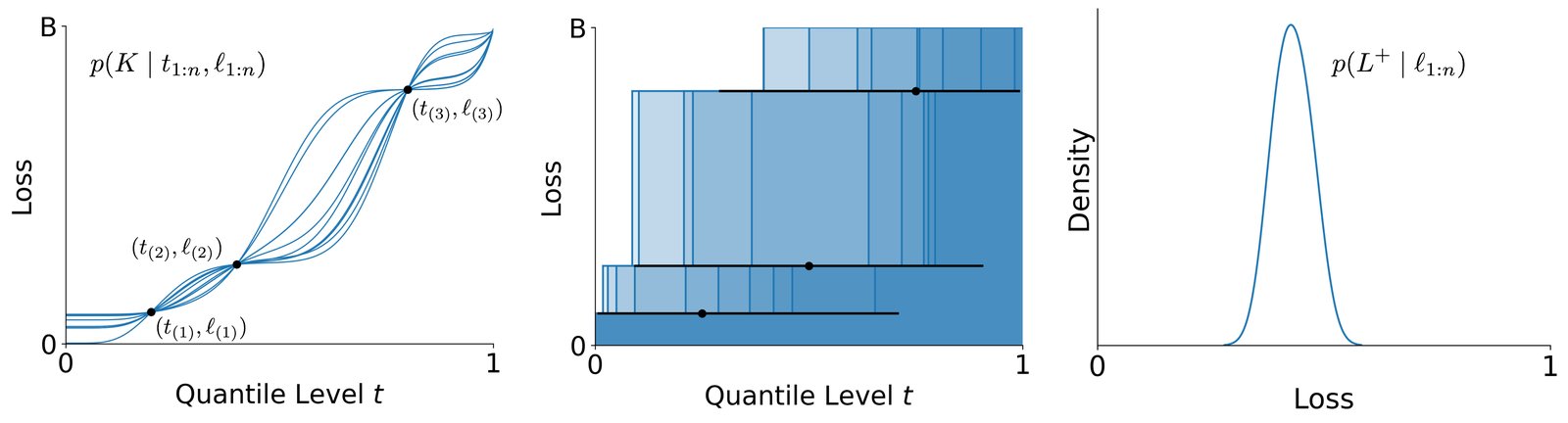
Figure 1: Overview of our approach. Left: Standard Bayesian quadrature places a prior over the quantile function of the loss distribution. The posterior is formed via Bayes’ rule after observing a set of loss values and quantile levels. However, in practice quantile levels are not directly observed. Middle: Our approach combines properties of quantile spacings with a right rectangular integration rule to construct an upper bound on the posterior distribution of the expected loss. Randomly sampled spacings and corresponding quantile functions are shown in blue along with a 95% credible interval for each quantile level in black. Right: The posterior distribution for a random variable $L^{+}$ that upper bounds the expected loss is constructed by integrating over the unknown quantile levels.

图 1：方法总览。左：标准贝叶斯求积在损失分布的分位数函数上放先验；观测一组损失值与分位水平后，经贝叶斯公式形成后验。但实践中分位水平并不直接可观测。中：我们的方法结合分位数间距性质与右矩形积分法则，构造期望损失后验分布的上界。蓝色显示随机采样的间距与对应分位数函数，黑色为各分位水平的 95% 可信区间。右：通过对未知分位水平积分，构造上界期望损失的随机变量 $L^{+}$ 的后验分布。

The posterior risk given the observed individual losses $\ell_{i}\triangleq\ell(z_{i},\lambda)$ for $i=1,\ldots,n$ becomes:

给定观测个体损失 $\ell_{i}\triangleq\ell(z_{i},\lambda)$（$i=1,\ldots,n$）后的后验风险成为：

$$E(L\mid\ell_{1:n})=\int J[K]p(K\mid\ell_{1:n})\,dK, \tag{23}$$

where $J[K]\triangleq\int_{0}^{1}K(t)\,dt$ and we have suppressed the dependence on $\lambda$ for notational convenience. The posterior over quantile functions can be expressed as:

其中 $J[K]\triangleq\int_{0}^{1}K(t)\,dt$，为记法简便已省略对 $\lambda$ 的依赖。分位数函数的后验可写成：

$$\displaystyle p(K\mid\ell_{1:n})=\int p(K\mid t_{1:n},\ell_{1:n})p(t_{1:n}\mid\ell_{1:n})\,dt_{1:n} \\ \displaystyle p(K\mid t_{1:n},\ell_{1:n})\propto\pi(K)\prod_{i=1}^{n}\delta(\ell_{i}-K(t_{i})). \tag{24}$$

This resembles the Bayesian quadrature problem from Section 2.2, except the evaluation sites $t_{1},\ldots,t_{n}$ are unknown. Fortunately, the distribution of $t_{1},\ldots,t_{n}$ is independent of the true distribution of the losses, as we shall now show.

这类似于第 2.2 节的贝叶斯求积问题，只是求值点 $t_{1},\ldots,t_{n}$ 未知。幸运的是，$t_{1},\ldots,t_{n}$ 的分布与损失的真实分布无关，如下所示。

4.3 Elimination of the Prior Distribution

4.3 消除先验分布

In order to address the dependence of the posterior risk on the prior $\pi(K)$, we derive an upper bound on the posterior expected loss. The bound takes the form of a weighted sum of the observed losses, where the weights are determined by the spacing between consecutive quantiles.

为处理后验风险对先验 $\pi(K)$ 的依赖，我们推导后验期望损失的上界。该界呈观测损失的加权和形式，权重由相邻分位数间距决定。

Theorem 4.1.

Let $t_{{(0)}}=0$, $t_{{(n+1)}}=1$, and $\ell_{{(n+1)}}=B$. Then

定理 4.1。

令 $t_{{(0)}}=0$，$t_{{(n+1)}}=1$，且 $\ell_{{(n+1)}}=B$。则

$$\sup_{\pi}E(L\mid t_{1:n},\ell_{1:n})\leq\sum_{i=1}^{n+1}u_{i}\ell_{{(i)}}, \tag{26}$$

where $u_{i}=t_{(i)}-t_{(i-1)}$.

其中 $u_{i}=t_{(i)}-t_{(i-1)}$。

Theorem 4.1 is based on the definite integral of the “worst-case” quantile function that is consistent with the observations. This strategy eliminates the need to specify a prior or evaluate an integral over functions $K$. We now turn our attention to handling the uncertainty over the quantiles $t_{1:n}$.

定理 4.1 基于与观测一致的「最坏情形」分位数函数的定积分。该策略无需指定先验，也无需对函数 $K$ 积分。接下来处理分位数 $t_{1:n}$ 的不确定性。

4.4 Random Quantile Spacings

4.4 随机分位数间距

We now appeal to a result about distribution-free tolerance regions that characterizes the distribution of spacings between consecutive ordered quantiles. Knowledge of this distribution will allow us to handle the input noise in the quadrature problem.

我们诉诸分布无关容许域的一个结果，它刻画相邻有序分位数之间间距的分布。知晓该分布后，就能处理求积问题中的输入噪声。

Lemma 4.2(Distribution of Quantile Spacings (Aitchison & Dunsmore, 1975, p. 140)).

Suppose that $\ell_{1},\ldots,\ell_{n}$ are drawn i.i.d. with continuous[^2] distribution function $F$. Let $t_{i}=F(\ell_{i})$ and $u_{i}=t_{(i)}-t_{(i-1)}$, where by convention $t_{(0)}=0$ and $t_{(n+1)}=1$. Then $(u_{1},u_{2},\ldots,u_{n+1})\cong\Dir(1,\ldots,1)$.

引理 4.2（分位数间距的分布（Aitchison & Dunsmore，1975，第 140 页））。

设 $\ell_{1},\ldots,\ell_{n}$ 独立同分布抽取，分布函数 $F$ 连续[2]。令 $t_{i}=F(\ell_{i})$ 且 $u_{i}=t_{(i)}-t_{(i-1)}$，约定 $t_{(0)}=0$、$t_{(n+1)}=1$。则 $(u_{1},u_{2},\ldots,u_{n+1})\cong\Dir(1,\ldots,1)$。

We are now ready to present our algorithm for bounding the expected loss $E(L\mid\ell_{1:n})$.

我们现可给出界定期望损失 $E(L\mid\ell_{1:n})$ 的算法。

4.5 Bound on Maximum Posterior Risk

4.5 最大后验风险的界

Putting together Lemma 4.2 and Theorem 4.1 allows us to bound the maximum posterior risk.

结合引理 4.2 与定理 4.1，即可界定最大后验风险。

Theorem 4.3.

Define $\ell_{(i)}$ to be the order statistics of $\ell_{1},\ldots,\ell_{n}$ for $i=1,\ldots,n$ and $\ell_{(n+1)}\triangleq B$. Let $L^{+}$ be the random variable defined as follows:

定理 4.3。

定义 $\ell_{(i)}$ 为 $\ell_{1},\ldots,\ell_{n}$ 的次序统计量（$i=1,\ldots,n$），并令 $\ell_{(n+1)}\triangleq B$。令 $L^{+}$ 为如下定义的随机变量：

$$U_{1},\ldots,U_{n+1}\sim\Dir(1,\ldots,1),\,L^{+}=\sum_{i=1}^{n+1}U_{i}\ell_{{(i)}}. \tag{27}$$

Then for any $b\in(-\infty,B]$,

则对任意 $b\in(-\infty,B]$，

$$\inf_{\pi}\Pr(L\leq b\mid\ell_{1:n})\geq\Pr(L^{+}\leq b). \tag{28}$$

Theorem 4.3 states that $L^{+}$ stochastically dominates the posterior risk, which allows us to directly form upper confidence bounds as follows.

定理 4.3 表明 $L^{+}$ 随机支配后验风险，从而可直接构造上置信界如下。

Corollary 4.4.

For any desired confidence level $\beta\in(0,1)$, define

推论 4.4。

对任意期望置信水平 $\beta\in(0,1)$，定义

$$b^{*}_{\beta}=\inf_{b}\{b:\Pr(L^{+}\leq b\mid\ell_{1:n})\geq\beta\}. \tag{29}$$

Then $\inf_{\pi}\Pr(L\leq b\mid\ell_{1:n})\geq\beta$ for any $b\geq b^{}_{\beta}$.*

则对任意 $b\geq b^{}{\beta}$，有$\inf{\pi}\Pr(L\leq b\mid\ell_{1:n})\geq\beta$。*

The critical value $b^{*}_{\beta}$ can be calculated by applying techniques for bounding linear combinations of Dirichlet random variables (Ng et al., 2011, p. 63). Alternatively, straightforward Monte Carlo simulation of $L^{+}$ is often sufficient, and is the approach we take in our experiments. An illustration is shown in Figure 2.

临界值 $b^{*}_{\beta}$ 可用界定 Dirichlet 随机变量线性组合的技术计算（Ng 等，2011，第 63 页）。也可对 $L^{+}$ 做直接蒙特卡洛模拟，这往往够用，也是我们实验中的做法。示意见图 2。

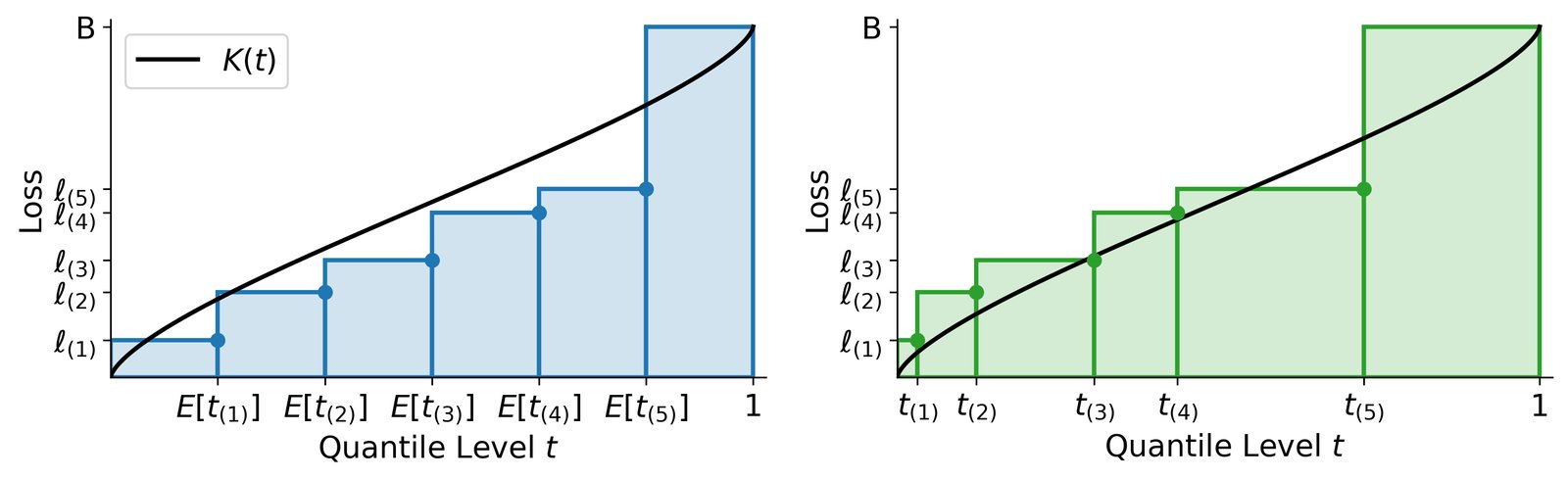
Figure 2: Our Bayesian approach to conformal prediction accounts for the variability in quantile levels better than previous approaches. Left: Conformal Risk Control (Angelopoulos et al., 2024) considers only the expectation over the unobserved quantile values $t_{1},\ldots,t_{n}$. This can underestimate the true expected loss (shown here: estimated expected loss $0.45$ vs. true expected loss $0.50$). Right: Our approach makes use of the fact that the quantile spacings are drawn from a Dirichlet distribution. By considering the full distribution over quantiles, we gain a more complete view of the expected loss. Shown here is one sample drawn from this distribution, which estimates the expected loss as $0.58$.

图 2：我们的共形预测贝叶斯方法比先前方法更好地计入分位水平的变异性。左：共形风险控制（Angelopoulos 等，2024）只考虑未观测分位值 $t_{1},\ldots,t_{n}$ 上的期望，可能低估真实期望损失（此处：估计期望损失 $0.45$，真实期望损失 $0.50$）。右：我们的方法利用分位数间距来自 Dirichlet 分布这一事实；通过考虑分位数的完整分布，对期望损失获得更完整的图景。图中展示从该分布抽取的一个样本，估计期望损失为 $0.58$。

4.6 Recovering Conformal Methods

4.6 恢复共形方法

This perspective puts the previous distribution-free uncertainty techniques in a new light. Taking the expected value of $L^{+}$, we find

这一视角让先前分布无关不确定性技术呈现新面貌。取 $L^{+}$ 的期望，得到

$$E(L^{+})=\sum_{i=1}^{n+1}E(U_{i})\ell_{(i)}=\frac{1}{n+1}\left(\sum_{i=1}^{n}\ell_{i}+B\right). \tag{30}$$

The Conformal Risk Control decision rule (15) then is simply the infimum over $\lambda$ for which $E(L^{+})\leq\alpha$.

共形风险控制决策规则（15）于是就是使 $E(L^{+})\leq\alpha$ 成立的 $\lambda$ 的下确界。

For, split conformal prediction, the individual loss is defined as $\ell_{i}=1-\mathbbm{1}\{s_{i}\leq\lambda\}$. Therefore, suppose that $\lambda=s_{(k)}$. The expected value of $L^{+}$ then becomes:

对分割共形预测，个体损失定义为 $\ell_{i}=1-\mathbbm{1}\{s_{i}\leq\lambda\}$。因此，设 $\lambda=s_{(k)}$，$L^{+}$ 的期望成为：

$$\displaystyle E(L^{+}) \\ \displaystyle=\frac{1}{n+1}\left(n+1-\sum_{i=1}^{n}\mathbbm{1}\{s_{i}\leq s_{(k)}\}\right) \\ \displaystyle=1-\frac{k}{n+1} \tag{31}$$

Therefore, $E(L^{+})\leq\alpha$ is satisfied whenever $k\geq(n+1)(1-\alpha)$, and in particular by $k^{*}=\lceil(n+1)(1-\alpha)\rceil$. This recovers (12) when $\lceil(n+1)(1-\alpha)\rceil\leq n$.

因此，每当 $k\geq(n+1)(1-\alpha)$，尤其取 $k^{*}=\lceil(n+1)(1-\alpha)\rceil$ 时，$E(L^{+})\leq\alpha$ 成立。当 $\lceil(n+1)(1-\alpha)\rceil\leq n$ 时，这恢复（12）。

Putting these results together, we have recovered standard conformal prediction techniques but have the additional flexibility of considering the distribution of $L^{+}$ rather than the expected value alone. Our experiments explore the value of this approach.

综合这些结果，我们恢复了标准共形预测技术，同时额外获得考虑 $L^{+}$ 分布而非仅期望的灵活性。实验将探讨这一做法的价值。

5 Experiments

5 实验

The primary goal of our experiments is to demonstrate the utility of producing a posterior distribution over the expected loss. We conduct experiments on both synthetic data and calibration data collected from MS-COCO (Lin et al., 2014). For each data setting, we randomly generate $M=$10true000$$ data splits. Each method is used to select $\lambda$ with the goal of controlling the risk such that $R(\theta,\lambda)\leq\alpha$ for unknown $\theta$. We compare algorithms on the basis of both the relative frequency of incurring risk greater than $\alpha$ and the prediction set size of the chosen $\lambda$. The ideal algorithm would select $\lambda$ such that the relative frequency of exceeding the target risk is at most a target failure rate of $1-\beta=0.05$ while minimizing prediction set size.

实验的主要目标是展示给出期望损失后验分布的用处。我们在合成数据以及从 MS-COCO（Lin 等，2014）收集的校准数据上实验。对每种数据设定，随机生成 $M=10{,}000$ 次数据划分。各方法用于选择 $\lambda$，目标是在未知 $\theta$ 下控制风险使 $R(\theta,\lambda)\leq\alpha$。我们从「风险超过 $\alpha$ 的相对频率」与所选 $\lambda$ 的预测集大小两方面比较算法。理想算法应选择使超过目标风险的相对频率至多为目标失败率 $1-\beta=0.05$，同时尽量缩小预测集。

As demonstrated in Section 4.6, our method recovers conformal risk control by taking the expected value of $L^{+}$. Therefore, in order to demonstrate the effect of targeting a conditional guarantee (as opposed to a marginal one as in conformal risk control), we use our Bayesian quadrature-based method to compute the decision rule based on the one-sided highest posterior density (HPD) interval:

如第 4.6 节所示，取 $L^{+}$ 的期望即可恢复共形风险控制。因此，为展示瞄准条件保证（相对共形风险控制的边际保证）的效果，我们用基于贝叶斯求积的方法，按单侧最高后验密度（HPD）区间计算决策规则：

$$\lambda^{\beta}_{\text{hpd}}\triangleq\inf_{\lambda}\{\lambda:\Pr(L^{+}\leq\alpha\mid\ell_{1:n})\geq\beta\}, \tag{33}$$

by finding the corresponding critical values $b_{\beta}^{*}$ according to (29) via Monte Carlo simulation of Dirichlet random variates with $1000$ samples. We include Risk-controlling Prediction Sets (RCPS) (Bates et al., 2021) with Hoeffding upper confidence bound as an additional baseline. Code for our experiments is publicly available on Github.[^3]

即按（29）经 1000 个 Dirichlet 随机变元的蒙特卡洛模拟求对应临界值 $b_{\beta}^{*}$。另以带 Hoeffding 上置信界的风险控制预测集（RCPS）（Bates 等，2021）为基线。实验代码已公开于 Github。[3]

5.1 Synthetic Binomial Data

5.1 合成二项数据

We first sample directly from a known loss distribution so that we can directly compute the frequency of excessively large risk. Here the loss distribution is chosen to be a scaled binomial distribution, normalized to have a maximum loss of $B=1$ and probability of failure set to $1-\lambda$. This was simulated by computing

我们先直接从已知损失分布抽样，以便直接计算风险过大的频率。此处损失分布选为缩放二项分布，归一化使最大损失 $B=1$，失败概率设为 $1-\lambda$。模拟时计算

$$\ell(z_{i},\lambda)=\frac{1}{K}\sum_{k=1}^{K}\mathbbm{1}\{V_{ik}>\lambda\}, \tag{34}$$

where $V_{ik}\sim\Uniform(0,1)$ for $i=1,\ldots,n$ and $k=1,\ldots,K$. This loss is therefore monotonically non-increasing in $\lambda$ and achieves zero loss at $\lambda_{\text{max}}=1$. We set $n$ = 10, $K=4$, and $\alpha=0.4$.

其中 $V_{ik}\sim\Uniform(0,1)$（$i=1,\ldots,n$，$k=1,\ldots,K$）。该损失对 $\lambda$ 单调非增，并在 $\lambda_{\text{max}}=1$ 时达到零损失。我们设 $n=10$，$K=4$，$\alpha=0.4$。

Since the expectation of the loss (34) is $1-\lambda$, any trial for which $\lambda<0.6$ constitutes a risk exceeding the $\alpha$ threshold. The relative frequency of trials exceeding this risk threshold are tabulated in Table 1.

由于损失（34）的期望为 $1-\lambda$，任何 $\lambda<0.6$ 的试验都构成超过 $\alpha$ 阈值的风险。超过该风险阈值的试验相对频率见表 1。

Decision Rule	Relative Freq.	95% CI
CRC	21.20%	[20.40%, 22.01%]
RCPS	0.00%	[0.00%, 0.04%]
Ours ($\beta=0.95$)	0.03%	[0.01%, 0.09%]

Table 1: Relative frequency of trials (out of 10,000) for which the resulting decision rule $\lambda$ exceeded the target risk threshold $\alpha$.

决策规则	相对频率	95% CI
CRC	21.20%	[20.40%, 22.01%]
RCPS	0.00%	[0.00%, 0.04%]
Ours ($\beta=0.95$)	0.03%	[0.01%, 0.09%]

表 1：在 10,000 次试验中，所得决策规则 $\lambda$ 超过目标风险阈值 $\alpha$ 的相对频率。

A histogram of the chosen $\lambda$ for each of the methods across all 10,000 trials is shown in Figure 3. For conformal risk control, the mean risk across all trials was $0.3363\pm 0.0007$ and for our approach $\lambda_{\text{hpd}}^{0.95}$ the mean risk was $0.1758\pm 0.0006$. In order to visualize the distribution of $L^{+}$, we plot a histogram of $L^{+}$ according to (27) estimated with 100,000 Dirichlet samples for three settings of $\lambda\in\{0.7,0.8,0.9\}$. The results are shown in Figure 4.

各方法在全部 10,000 次试验中所选 $\lambda$ 的直方图见图 3。共形风险控制的跨试验平均风险为 $0.3363\pm 0.0007$，本方法 $\lambda_{\text{hpd}}^{0.95}$ 的平均风险为 $0.1758\pm 0.0006$。为可视化 $L^{+}$ 的分布，我们按（27）用 100,000 个 Dirichlet 样本，对 $\lambda\in\{0.7,0.8,0.9\}$ 三种设定绘制 $L^{+}$ 直方图，结果见图 4。

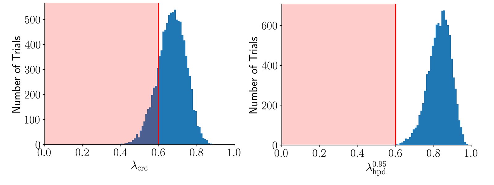
Figure 3: Comparison of risk incurred by each procedure across multiple trials. Left: Histogram of the decision rule $\lambda_{\text{crc}}$ chosen by Conformal Risk Control across $M$ = 10,000 randomly sampled calibration sets. The region where per-trial risk exceeds $\alpha$ is highlighted in red. Right: Histogram of the $\lambda_{\text{hpd}}^{0.95}$ chosen according to our 95% Bayesian posterior interval.

图 3：各程序跨多次试验所招致风险的比较。左：共形风险控制在 $M=10{,}000$ 个随机校准集上所选决策规则 $\lambda_{\text{crc}}$ 的直方图；单次试验风险超过 $\alpha$ 的区域以红色标出。右：按我们 95% 贝叶斯后验区间所选 $\lambda_{\text{hpd}}^{0.95}$ 的直方图。

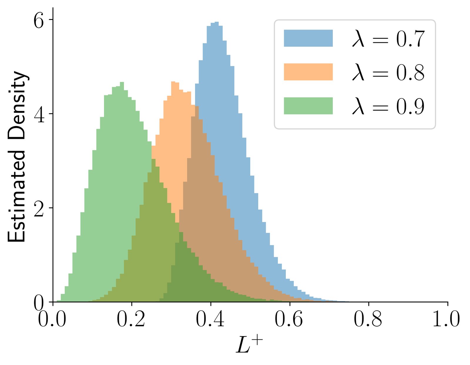
Figure 4: Probability density for $L^{+}$ with $\lambda\in\{0.7,0.8,0.9\}$ estimated using 100,000 Dirichlet samples.

图 4：用 100,000 个 Dirichlet 样本估计的 $L^{+}$ 概率密度，$\lambda\in\{0.7,0.8,0.9\}$。

5.2 Synthetic Heteroskedastic Data

5.2 合成异方差数据

In this experiment we also use 10,000 random trials. We use $n=200$ calibration samples each. To achieve heteroskedasticity, we let $X\sim U[0,4]$ and $Y\mid X\sim\mathcal{N}(0,X^{2})$. The prediction intervals are then formed as $[-\hat{\lambda},\hat{\lambda}]$ where $\hat{\lambda}$ is selected by each method. The loss is the miscoverage loss and the target loss is set to $\alpha=0.1$ (i.e. 90% coverage). The maximum allowable risk failure rate is set to 5% (i.e. $\beta=0.95$). The results are show in Table 2.

本实验同样使用 10,000 次随机试验，每次 $n=200$ 个校准样本。为实现异方差，令 $X\sim U[0,4]$，$Y\mid X\sim\mathcal{N}(0,X^{2})$。预测区间取为 $[-\hat{\lambda},\hat{\lambda}]$，其中 $\hat{\lambda}$ 由各方法选定。损失为未覆盖损失，目标损失设为 $\alpha=0.1$（即 90% 覆盖）。最大允许风险失败率设为 5%（即 $\beta=0.95$）。结果见表 2。

Decision Rule	Relative Freq.	95% CI	Mean Prediction Interval Length
Split Conformal Prediction / CRC	46.19%	[45.21%, 47.17%]	7.99
RCPS	0.0%	[0.0%, 0.04%]	14.29
Ours ($\beta=0.95$)	3.42%	[3.07%, 3.80%]	9.50

Table 2: Relative frequency of trials (out of 10,000) for which the resulting decision rule $\lambda$ exceeded the target risk threshold $\alpha$ in the synthetic heteroskedastic experiment.

决策规则	相对频率	95% CI	平均预测区间长度
Split Conformal Prediction / CRC	46.19%	[45.21%, 47.17%]	7.99
RCPS	0.0%	[0.0%, 0.04%]	14.29
Ours ($\beta=0.95$)	3.42%	[3.07%, 3.80%]	9.50

表 2：合成异方差实验中，所得决策规则 $\lambda$ 超过目标风险阈值 $\alpha$ 的试验相对频率（共 10,000 次）。

5.3 False Negative Rate on MS-COCO

5.3 MS-COCO 上的假阴性率

We also compare methods on controlling the false negative rate of multilabel classification on the MS-COCO dataset (Lin et al., 2014). The experimental setup mirrors that used by Angelopoulos & Bates (2023, Section 5.1). Each random split contains $1000$ calibration examples and $3952$ test examples. The results of this experiment are summarized in Table 3.

我们还在 MS-COCO 数据集（Lin 等，2014）上比较各方法对多标签分类假阴性率的控制。实验设置与 Angelopoulos & Bates（2023，第 5.1 节）一致。每次随机划分含 1000 个校准样本与 3952 个测试样本。结果汇总于表 3。

Method	Relative Freq.	Pred. Set Size
CRC	45.05%	2.92
RCPS	0.0%	3.57
Ours ($\beta=0.95$)	5.43%	3.04

Table 3: Results on MS-COCO comparing relative frequency of trials for which the resulting decision rule $\lambda$ exceeded the target risk threshold $\alpha$ and average prediction set size.

方法	相对频率	预测集大小
CRC	45.05%	2.92
RCPS	0.0%	3.57
Ours ($\beta=0.95$)	5.43%	3.04

表 3：MS-COCO 上比较所得决策规则 $\lambda$ 超过目标风险阈值 $\alpha$ 的试验相对频率与平均预测集大小。

6 Discussion

6 讨论

Our results in Table 1 demonstrate that even though the Conformal Risk Control marginal guarantee holds, a significant number of individual trials (21.20%) may incur risk exceeding the target threshold. In contrast, by using the more conservative HPD criterion, very few of the trials (0.03%) exceeded the target risk. In Table 2, both RCPS and our method achieve failure rate below the target of 5% but our method achieves significantly smaller prediction intervals.

表 1 结果表明：即便共形风险控制的边际保证成立，仍有相当比例的单次试验（21.20%）可能招致超过目标阈值的风险。相比之下，采用更保守的 HPD 准则后，极少试验（0.03%）超过目标风险。表 2 中 RCPS 与本方法都把失败率压到 5% 目标以下，但本方法得到的预测区间显著更短。

These results point to the qualitative difference in a marginal guarantee, which averages over many possible yet unobserved data sets vs. a conditional guarantee which focuses on knowledge about the state of nature conditioned on the calibration data actually observed. Previous work on conditional guarantees (Barber et al., 2021; Gibbs et al., 2024) has focused on input-conditional guarantees, where the guarantee is conditioned on for all in the input domain. Guarantees of this nature have been shown to be generally impossible without stronger distribution assumptions. Our guarantees are perhaps better characterized by the term “data-conditional guarantee”, where we condition on the set of observed loss values. Our experiments demonstrate the practical benefits of this by achieving decisions that produce smaller prediction sets and intervals while not violating the constraint on maximum allowable failure rate. Our guarantees, in contrast, do not rely on strong distribution assumptions that would be necessary to produce an input-conditional guarantee.

这些结果指向边际保证与条件保证的质的差别：前者对许多可能但未观测的数据集取平均，后者聚焦于条件于实际观测校准数据后关于自然状态的知识。先前关于条件保证的工作（Barber 等，2021；Gibbs 等，2024）多关注输入条件保证，即对输入域中所有点成立的保证；已证明在没有更强分布假设时这类保证通常不可能。我们的保证或许更适合称为「数据条件保证」——条件于观测损失值集合。实验表明其实际好处：在不违反最大允许失败率约束的前提下，得到更小的预测集与区间。我们的保证也不依赖产生输入条件保证所必需的强分布假设。

The results are again confirmed in Table 3 on MS-COCO, which show that the marginal guarantees of Conformal Risk Control lead to an even greater percentage of trials exceeding the risk threshold. On the other hand, RCPS is able to control the risk but this comes at the cost of larger prediction sets. Our approach successfully balances these two concerns, producing prediction intervals that are shorter than baselines while not exceeding the maximum acceptable failure rate. It is also clear that the distribution of the expected loss upper bound $L^{+}$ in Figure 4 provides a more complete view of the range of possible losses and its dependence on $\lambda$, a perspective that is not offered by previous methods.

表 3 的 MS-COCO 结果再次确认：共形风险控制的边际保证会导致更高比例试验超过风险阈值。另一方面，RCPS 能控制风险，但代价是更大的预测集。本方法在二者之间取得平衡：预测区间短于基线，同时不超过最大可接受失败率。图 4 中期望损失上界 $L^{+}$ 的分布也清楚表明，它对可能损失范围及其对 $\lambda$ 的依赖给出更完整图景，这是先前方法所不具备的视角。

Our goal in this work is to show that the Bayesian viewpoint unlocks a richer interpretation compared to previous works, which focus on marginal guarantees that as we have shown in the paper correspond to the posterior mean. In order to draw an explicit correspondence between our work and previous approaches, the dependence on the prior was removed in Section 4.3. The intuition is that that any rational decision maker operating according to the rules of probability, regardless of prior (sufficiently expressive), would agree with the upper-bounding distribution of we derive. Naturally, commitment to a specific choice of prior would lead to tighter distributions over the posterior risk, and in future work we seek to bridge these fields even further by exploring specific choices of priors over quantile functions.

本文目标是表明贝叶斯观点能解锁比先前工作更丰富的解释——后者聚焦于边际保证，我们已说明其对应于后验均值。为与先前方法建立显式对应，第 4.3 节去掉了对先验的依赖。直觉是：任何按概率规则运作的理性决策者，无论先验如何（只要足够表达力强），都会认同我们导出的上界分布。自然地，承诺特定先验会得到对后验风险更紧的分布；未来工作希望进一步衔接这些领域，探索分位数函数上的具体先验选择。

The limitations of our method lie primarily in the two main assumptions it makes. First, it assumes that the data at deployment time are independent and identically distributed to the calibration data. Second, it assumes an upper bound $B$ on the losses. If either of these assumptions do not hold, then the guarantees produced by our method are no longer valid. Additionally, the bounds produced by our method are conservative in the sense that they hold for any choice of prior for the loss distribution (provided that the prior is consistent with the calibration data). Therefore, if the two aforementioned assumptions do hold, the actual loss values may be significantly less than indicated by our method.

方法局限主要在于两条假设。第一，假定部署时数据与校准数据独立同分布。第二，假定损失有上界 $B$。任一假设不成立，方法给出的保证就不再有效。此外，我们的界对损失分布的任意先验选择都成立（只要先验与校准数据一致），因而偏保守；若上述两条假设成立，实际损失可能显著低于方法所示。

Overall, our approach demonstrates how conformal prediction techniques can be recovered and extended using Bayesian probability, all without having to specify a prior distribution. This Bayesian formulation is highly flexible due to its nonparametric nature, yet is amenable to incorporating specific information about the distribution of losses likely to be encountered. In practical applications, maximizing the risk with respect to all possible priors may be too conservative, and thus future work may explore the effect of specific priors on the risk estimate.

总体而言，本方法表明：无须指定先验分布，即可用贝叶斯概率恢复并扩展共形预测技术。该贝叶斯表述因其非参数性质而高度灵活，同时又便于融入关于可能遇到的损失分布的具体信息。实践中，相对所有可能先验最大化风险可能过于保守，未来工作可探索特定先验对风险估计的影响。

7 Related Work

7 相关工作

Statistical Prediction Analysis.

Statistical prediction analysis (Aitchison & Dunsmore, 1975) deals with the use of statistical inference to reason about the likely outcomes of future prediction tasks given past ones. Within statistical prediction analysis, the area of distribution-free prediction assumes that the parameters or the form of the distributions involved cannot be identified. This idea can be traced back to Wilks (1941), who constructed a method to form distribution-free tolerance regions. Tukey (1947); Tukey (1948) generalized distribution-free tolerance regions and introduced the concept of statistically equivalent blocks, which are analogous to the intervals between consecutive order statistics of the losses. Much of the relevant theory is summarized by Guttman (1970), and the Dirichlet distribution of quantile spacing is discussed by Aitchison & Dunsmore (1975). We build upon these works by connecting them to Bayesian quadrature and applying them in the more modern context of distribution-free uncertainty quantification.

统计预测分析。

统计预测分析（Aitchison & Dunsmore，1975）研究如何用统计推断，在已有预测任务基础上推断未来预测任务的可能结果。其中，分布无关预测假定所涉分布的参数或形式不可识别。这一思想可追溯到 Wilks（1941）构造分布无关容许域的方法。Tukey（1947；1948）推广了分布无关容许域，并引入统计等价块概念，类似于损失次序统计量之间的区间。相关理论多由 Guttman（1970）总结，分位数间距的 Dirichlet 分布则见 Aitchison & Dunsmore（1975）。我们在这些工作之上，把它们接到贝叶斯求积，并应用到更现代的分布无关不确定性量化语境。

Bayesian Quadrature.

The use of Bayesian probability to represent the outcome of a arbitrary computation is termed probabilistic numerics (Cockayne et al., 2019; Hennig et al., 2022). Since our approach is fundamentally based on integration, we focus primarily on the relationship with the more narrow approach of Bayesian quadrature, which employs Bayes rule to estimate the value of an integral. A lucid overview of this approach is discussed under the term Bayesian numerical analysis by Diaconis (1988), who traces it back to the late nineteenth century (Poincaré, 1896). The use of Gaussian processes in performing Bayesian quadrature is discussed in detail by O’Hagan (1991). Our approach is formulated similarly but differs in two main ways: (a) we use a conservative bound instead of an explicit prior, and (b) we have input noise induced by the random quantile spacings.

贝叶斯求积。

用贝叶斯概率表示任意计算结果的做法称为概率数值（Cockayne 等，2019；Hennig 等，2022）。由于本方法本质上基于积分，我们主要关注与更狭义的贝叶斯求积的关系——后者用贝叶斯法则估计积分值。Diaconis（1988）在贝叶斯数值分析名义下给出清晰综述，并将其追溯到十九世纪末（Poincaré，1896）。用高斯过程做贝叶斯求积由 O’Hagan（1991）详细讨论。我们的表述类似，但有两点不同：（a）用保守界代替显式先验；（b）存在由随机分位数间距诱导的输入噪声。

Distribution-Free Uncertainty Quantification.

Relevant background on distribution-free uncertainty quantification techniques is discussed in Section 2.1. A recent and comprehensive introduction to conformal prediction and related techniques may be found in (Angelopoulos & Bates, 2023). Some recent works, like ours, also make use of quantile functions (Snell et al., 2023; Farzaneh et al., 2024) but remain grounded in frequentist probability. Separately, Bayesian approaches to predictive uncertainty are popular (Hobbhahn et al., 2022) but make extensive assumptions about the form of the underlying predictive model. To our knowledge, we are the first to apply statistical prediction analysis and Bayesian quadrature in order to analyze the performance of black-box predictive models in a distribution-free way.

分布无关不确定性量化。

分布无关不确定性量化技术的相关背景见第 2.1 节。共形预测及相关技术的近期全面导论见 Angelopoulos & Bates（2023）。若干近期工作与我们一样使用分位数函数（Snell 等，2023；Farzaneh 等，2024），但仍立足频率派概率。另一方面，预测不确定性的贝叶斯方法很流行（Hobbhahn 等，2022），但对底层预测模型形式做了大量假设。据我们所知，我们是首次把统计预测分析与贝叶斯求积用于以分布无关方式分析黑盒预测模型表现。

8 Conclusion

8 结论

Safely deploying black-box predictive models, such as those based on deep neural networks, requires developing methods that provide guarantees of their performance. Existing techniques for solving this problem are based on frequentist statistics, and are thus difficult to extend to incorporate knowledge about the situation in which models may be deployed. In this work we provided a Bayesian alternative to distribution-free uncertainty quantification, showing that two popular existing methods are special cases of this approach. Our results show that Bayesian probability can be used to extend uncertainty quantification techniques, making their underlying assumptions more explicit, allowing incorporation of additional knowledge, and providing a more intuitive foundation for constructing performance guarantees that avoid overly-optimistic guarantees that can be produced by existing methods.

安全部署基于深度神经网络等黑盒预测模型，需要能对其表现给出保证的方法。解决该问题的既有技术基于频率派统计，因而难以扩展以融入关于模型部署情境的知识。本文给出分布无关不确定性量化的贝叶斯替代，并表明两种流行既有方法都是本方法的特例。结果表明：贝叶斯概率可用于扩展不确定性量化技术，使其底层假设更显式，允许融入额外知识，并为构造表现保证提供更直观的基础，从而避免既有方法可能产生的过于乐观的保证。

Impact Statement

影响声明

This paper introduces a practical algorithm for computing a posterior distribution for the expected loss based on the observed losses from a set of calibration data. The intended purpose of this algorithm is for the posterior distribution to inform deployment decisions of black-box predictive systems (e.g. deep neural networks) in safety-critical applications. Our method makes use of certain assumptions, discussed in Section 6, which if violated will lead to guarantees that may no longer hold. In particular, it is important to ensure proper monitoring to detect distribution shift between calibration and deployment.

本文引入一种实用算法：基于校准数据观测到的损失，计算期望损失的后验分布。算法意图是用此后验分布指导安全关键应用中黑盒预测系统（如深度神经网络）的部署决策。方法依赖第 6 节讨论的若干假设；若假设被违反，保证可能不再成立。尤其需要妥善监控，以检测校准与部署之间的分布偏移。

Acknowledgements

致谢

The authors would like to thank the anonymous reviewers for helpful comments. This work was supported by grant N00014-23-1-2510 from the Office of Naval Research.

作者感谢匿名审稿人的有益意见。本研究获美国海军研究办公室资助 N00014-23-1-2510 支持。

References

参考文献

Aitchison & Dunsmore (1975) Aitchison, J. and Dunsmore, I. R. Statistical Prediction Analysis . New York: Cambridge University Press, 1975.

Angelopoulos & Bates (2023) Angelopoulos, A. N. and Bates, S. Conformal prediction: A gentle introduction. Foundations and Trends in Machine Learning , 16(4):494–591, 2023.

Angelopoulos et al. (2024) Angelopoulos, A. N., Bates, S., Fisch, A., Lei, L., and Schuster, T. Conformal risk control. In The Twelfth International Conference on Learning Representations , 2024.

Barber et al. (2021) Barber, R. F., Candès, E. J., Ramdas, A., and Tibshirani, R. J. The limits of distribution-free conditional predictive inference. Information and Inference: A Journal of the IMA , 10(2):455–482, June 2021. ISSN 2049-8772. doi: 10.1093/imaiai/iaaa017 .

Bates et al. (2021) Bates, S., Angelopoulos, A., Lei, L., Malik, J., and Jordan, M. Distribution-free, risk-controlling prediction sets. Journal of the ACM , 68(6), 2021.

Cockayne et al. (2019) Cockayne, J., Oates, C. J., Sullivan, T. J., and Girolami, M. Bayesian probabilistic numerical methods. SIAM Review , 61(3):756–789, 2019.

Diaconis (1988) Diaconis, P. Bayesian numerical analysis. In Berger, J. and Gupta, S. (eds.), Statistical Decision Theory and Related Topics IV , volume 1, pp. 163–175. Springer-Verlag, 1988.

Farzaneh et al. (2024) Farzaneh, A., Park, S., and Simeone, O. Quantile learn-then-test: Quantile-based risk control for hyperparameter optimization. IEEE Signal Processing Letters , 2024.

Gibbs et al. (2024) Gibbs, I., Cherian, J. J., and Candès, E. J. Conformal Prediction With Conditional Guarantees, September 2024.

Guttman (1970) Guttman, I. Statistical Tolerance Regions: Classical and Bayesian . Griffin’s Statistical Monographs and Courses, No. 26. Griffin, 1970.

Hennig et al. (2022) Hennig, P., Osborne, M. A., and Kersting, H. P. Probabilistic Numerics: Computation as Machine Learning . Cambridge University Press, 2022.

Hobbhahn et al. (2022) Hobbhahn, M., Kristiadi, A., and Hennig, P. Fast predictive uncertainty for classification with Bayesian deep networks. In Proceedings of the Thirty-Eighth Conference on Uncertainty in Artificial Intelligence , 2022.

Karvonen & Särkkä (2017) Karvonen, T. and Särkkä, S. Classical quadrature rules via Gaussian processes. In 2017 IEEE 27th International Workshop on Machine Learning for Signal Processing (MLSP) , 2017.

Kot (2014) Kot, M. A First Course in the Calculus of Variations . American Mathematical Society, 2014.

Lei et al. (2018) Lei, J., G’Sell, M., Rinaldo, A., Tibshirani, R. J., and Wasserman, L. Distribution-free predictive inference for regression. Journal of the American Statistical Association , 113(523):1094–1111, July 2018.

Lin et al. (2014) Lin, T.-Y., Maire, M., Belongie, S., Hays, J., Perona, P., Ramanan, D., Dollár, P., and Zitnick, C. L. Microsoft COCO: Common objects in context. In 13th European Conference on Computer Vision , pp. 740–755. Springer, 2014.

Ng et al. (2011) Ng, K. W., Tian, G.-L., and Tang, M.-L. Dirichlet and Related Distributions: Theory, Methods and Applications . Wiley, 2011.

O’Hagan (1991) O’Hagan, A. Bayes–Hermite quadrature. Journal of Statistical Planning and Inference , 29(3):245–260, November 1991.

Papadopoulos et al. (2002) Papadopoulos, H., Proedrou, K., Vovk, V., and Gammerman, A. Inductive confidence machines for regression. In Elomaa, T., Mannila, H., and Toivonen, H. (eds.), ECML 2002 , volume 2430, pp. 345–356. Springer Berlin Heidelberg, 2002.

Poincaré (1896) Poincaré, H. Calcul des Probabilités . Georges Carré, 1896.

Shafer & Vovk (2008) Shafer, G. and Vovk, V. A tutorial on conformal prediction. Journal of Machine Learning Research , 9(12):371–421, 2008.

Shao (2003) Shao, J. Mathematical Statistics . Springer, 2003.

Shorack (2000) Shorack, G. Probability for Statisticians . Springer-Verlag, 2000.

Shorack & Wellner (2009) Shorack, G. R. and Wellner, J. A. Empirical Processes with Applications to Statistics . Society for Industrial and Applied Mathematics, 2009.

Snell et al. (2023) Snell, J. C., Zollo, T. P., Deng, Z., Pitassi, T., and Zemel, R. Quantile risk control: A flexible framework for bounding the probability of high-loss predictions. In The Eleventh International Conference on Learning Representations , 2023.

Tukey (1947) Tukey, J. W. Nonparametric estimation II. Statistically equivalent blocks and tolerance regions–the continuous case. The Annals of Mathematical Statistics , pp. 529–539, 1947.

Tukey (1948) Tukey, J. W. Nonparametric estimation, III. Statistically equivalent blocks and multivariate tolerance regions–the discontinuous case. The Annals of Mathematical Statistics , pp. 30–39, 1948.

Vovk et al. (2005) Vovk, V., Gammerman, A., and Shafer, G. Algorithmic Learning in a Random World . Springer Science & Business Media, 2005.

Wilks (1941) Wilks, S. S. Determination of sample sizes for setting tolerance limits. The Annals of Mathematical Statistics , 12(1):91–96, 1941.

Appendix A Theoretical Preliminaries

附录 A 理论预备

A.1 Review of Problem Setup

A.1 问题设定回顾

We first review some relevant aspects of our problem setup.

我们先回顾问题设定中若干相关方面。

Loss Function.

We assume an upper bound on the losses: $\ell_{i}\in(-\infty,B]$ for $i=1,\ldots,n$. We assume the same upper bound for $\ell_{\text{new}}$.

损失函数。

我们假定损失有上界：$\ell_{i}\in(-\infty,B]$（$i=1,\ldots,n$）。对 $\ell_{\text{new}}$ 假定同一上界。

Bayesian Quadrature of Quantile Functions.

Recall Bayes rule for quantile functions:

分位数函数的贝叶斯求积。

回顾分位数函数的贝叶斯法则：

$$p(K\mid t_{1:n},\ell_{1:n})\propto\pi(K)\prod_{i=1}^{n}\delta(\ell_{i}-K(t_{i})), \tag{35}$$

where $\delta$ is the Dirac delta function. The prior $\pi(K)$ is assumed to be sufficiently expressive to have nonzero measure for the set $\mathcal{K}_{n}$ of quantile functions such that $K(t_{i})=\ell_{i}$ for $i=1,\ldots,n$ and $K\in\mathcal{K}_{n}$. This is necessary to prevent the posterior distribution in (35) from becoming degenerate.

其中 $\delta$ 是 Dirac δ 函数。假定先验 $\pi(K)$ 足够表达力强，使满足 $K(t_{i})=\ell_{i}$（$i=1,\ldots,n$）且 $K\in\mathcal{K}_{n}$ 的分位数函数集合 $\mathcal{K}_{n}$ 具有非零测度。这是为了防止（35）中的后验分布退化。

A.2 Background

A.2 背景

We begin by recalling some basic properties of distribution functions and quantile functions.

我们先回忆分布函数与分位数函数的一些基本性质。

Proposition A.1(Properties of Distribution Functions (Shao, 2003, p. 4)).

Let $F(x)=\Pr(X\leq x)$ be a distribution function. Then $F(-\infty)=\lim_{x\rightarrow-\infty}F(x)=0$, $F(\infty)=\lim_{x\rightarrow\infty}F(x)=1$, $F$ is nondecreasing (i.e., $F(x)\leq F(y)$ if $x\leq y$), and $F$ is right continuous (i.e., $\lim_{y\rightarrow x,y>x}F(y)=F(x)$).

命题 A.1（分布函数的性质（Shao，2003，第 4 页））。

令 $F(x)=\Pr(X\leq x)$ 为分布函数。则 $F(-\infty)=\lim_{x\rightarrow-\infty}F(x)=0$，$F(\infty)=\lim_{x\rightarrow\infty}F(x)=1$，$F$ 非减（即若 $x\leq y$ 则 $F(x)\leq F(y)$），且 $F$ 右连续（即 $\lim_{y\rightarrow x,y>x}F(y)=F(x)$）。

Let $F$ be a distribution function and $K(t)\equiv F^{-1}(t)=\inf\{x:F(x)\geq t\}$ be the corresponding quantile function.

令 $F$ 为分布函数，$K(t)\equiv F^{-1}(t)=\inf\{x:F(x)\geq t\}$ 为对应分位数函数。

Proposition A.2(Quantile Functions are Nondecreasing).

If $t\leq u$, then $K(t)\leq K(u)$.

命题 A.2（分位数函数非减）。

若 $t\leq u$，则 $K(t)\leq K(u)$。

Proof.

Since $u\geq t$, it follows that $\{x:F(x)\geq u\}\subseteq\{x:F(x)\geq t\}$. Taking the infimum of both sides yields

证明。

由于 $u\geq t$，有 $\{x:F(x)\geq u\}\subseteq\{x:F(x)\geq t\}$。两边取下确界得

$$\inf\{x:F(x)\geq u\}\geq\inf\{x:F(x)\geq t\}\Rightarrow K(u)\geq K(t). \tag{36}$$

∎

We also will make use of the probability integral transformation, which we state here for convenience.

我们还将用到概率积分变换，为方便起见陈述如下。

Proposition A.3(Probability Integral Transformation (Shorack & Wellner, 2009, p. 5)).

If $X$ has distribution function $F$, then

命题 A.3（概率积分变换（Shorack & Wellner，2009，第 5 页））。

若 $X$ 有分布函数 $F$，则