Convolutional Neural Networks for Sentence Classification
Convolutional Neural Networks for Sentence Classification
用于句子分类的卷积神经网络
Yoon Kim Affiliation: New York University Email: yhk255@nyu.edu
Abstract
摘要
We report on a series of experiments with convolutional neural networks (CNN) trained on top of pre-trained word vectors for sentence-level classification tasks. We show that a simple CNN with little hyperparameter tuning and static vectors achieves excellent results on multiple benchmarks. Learning task-specific vectors through fine-tuning offers further gains in performance. We additionally propose a simple modification to the architecture to allow for the use of both task-specific and static vectors. The CNN models discussed herein improve upon the state of the art on 4 out of 7 tasks, which include sentiment analysis and question classification.
我们报告了一系列实验:在预训练词向量之上训练卷积神经网络(CNN),用于句子级分类任务。结果表明,超参几乎不做调优、词向量保持静态的简单 CNN,就能在多个基准上取得出色结果;再通过微调学习任务相关向量,还能继续抬分。我们还对结构做了一处简单修改,使任务相关向量与静态向量可以同时使用。本文讨论的 CNN 在 7 项任务中的 4 项上超过了当时最优结果,覆盖情感分析与问题分类等。
1 Introduction
1 引言
Deep learning models have achieved remarkable results in computer vision [2012] and speech recognition [2013] in recent years. Within natural language processing, much of the work with deep learning methods has involved learning word vector representations through neural language models (Bengio et al., 2003; Yih et al., 2011; Mikolov et al., 2013) and performing composition over the learned word vectors for classification [2011]. Word vectors, wherein words are projected from a sparse, 1-of- encoding (here is the vocabulary size) onto a lower dimensional vector space via a hidden layer, are essentially feature extractors that encode semantic features of words in their dimensions. In such dense representations, semantically close words are likewise close—in euclidean or cosine distance—in the lower dimensional vector space.
近年来,深度学习模型在计算机视觉 [2012] 与语音识别 [2013] 上取得了显著成果。在自然语言处理中,大量工作围绕通过神经语言模型学习词向量表示(Bengio et al., 2003;Yih et al., 2011;Mikolov et al., 2013),再对学到的词向量做组合以完成分类 [2011]。所谓词向量,是把词从稀疏的 one-of- 编码( 为词表大小)经由隐层投影到低维向量空间;本质上是特征抽取器,在各个维度上编码语义特征。在这种稠密表示里,语义相近的词在低维空间中(欧氏距离或余弦距离)也彼此靠近。
Convolutional neural networks (CNN) utilize layers with convolving filters that are applied to local features [1998]. Originally invented for computer vision, CNN models have subsequently been shown to be effective for NLP and have achieved excellent results in semantic parsing [2014], search query retrieval [2014], sentence modeling [2014], and other traditional NLP tasks [2011].
卷积神经网络(CNN)使用卷积滤波器层,把滤波器施加到局部特征上 [1998]。CNN 最初为计算机视觉提出,随后被证明对 NLP 同样有效,并在语义解析 [2014]、搜索查询检索 [2014]、句子建模 [2014] 以及其他传统 NLP 任务 [2011] 上取得了出色结果。
In the present work, we train a simple CNN with one layer of convolution on top of word vectors obtained from an unsupervised neural language model. These vectors were trained by Mikolov et al. [2013] on 100 billion words of Google News, and are publicly available.[^1] We initially keep the word vectors static and learn only the other parameters of the model. Despite little tuning of hyperparameters, this simple model achieves excellent results on multiple benchmarks, suggesting that the pre-trained vectors are ‘universal’ feature extractors that can be utilized for various classification tasks. Learning task-specific vectors through fine-tuning results in further improvements. We finally describe a simple modification to the architecture to allow for the use of both pre-trained and task-specific vectors by having multiple channels.
本文在无监督神经语言模型得到的词向量之上,训练仅含一层卷积的简单 CNN。这些向量由 Mikolov et al. [2013] 在 1000 亿词的 Google News 上训练,并可公开获取。[^1] 我们先把词向量固定为静态,只学习模型其余参数。尽管超参几乎未调,这一简单模型已在多个基准上表现优异,说明预训练向量可作为可复用的「通用」特征抽取器,服务多种分类任务。通过微调学习任务相关向量还能进一步提升。最后,我们描述对结构的一处简单修改:用多通道同时使用预训练向量与任务相关向量。
Our work is philosophically similar to Razavian et al. [2014] which showed that for image classification, feature extractors obtained from a pre-trained deep learning model perform well on a variety of tasks—including tasks that are very different from the original task for which the feature extractors were trained.
我们的思路在理念上与 Razavian et al. [2014] 相近:该工作表明,从预训练深度学习模型得到的特征抽取器,在图像分类的多种任务上表现良好——包括与当初训练这些抽取器的任务差异很大的任务。
2 Model
2 模型
The model architecture, shown in figure 1, is a slight variant of the CNN architecture of Collobert et al. [2011]. Let be the -dimensional word vector corresponding to the -th word in the sentence. A sentence of length (padded where necessary) is represented as
模型结构如图 1 所示,是 Collobert et al. [2011] CNN 结构的轻微变体。令 为句子中第 个词对应的 维词向量。长度为 的句子(必要时做填充)表示为
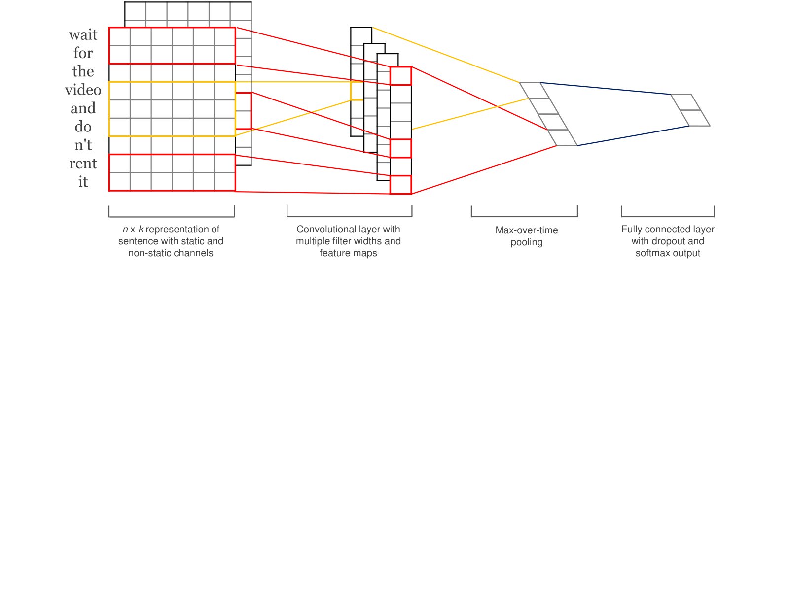
Figure 1: Model architecture with two channels for an example sentence.
图 1:示例句子上的双通道模型结构。
where is the concatenation operator. In general, let refer to the concatenation of words . A convolution operation involves a filter , which is applied to a window of words to produce a new feature. For example, a feature is generated from a window of words by
其中 为拼接算子。一般地,令 表示词 的拼接。卷积操作使用一个 滤波器 ,作用于长度为 的词窗口以产生新特征。例如,由窗口 生成特征 的方式为
Here is a bias term and is a non-linear function such as the hyperbolic tangent. This filter is applied to each possible window of words in the sentence to produce a feature map
这里 是偏置项, 是非线性函数(如双曲正切)。该滤波器作用于句子中每一个可能的词窗口 ,得到 特征图
with . We then apply a max-over-time pooling operation [2011] over the feature map and take the maximum value as the feature corresponding to this particular filter. The idea is to capture the most important feature—one with the highest value—for each feature map. This pooling scheme naturally deals with variable sentence lengths.
其中 。接着对特征图做 max-over-time 池化 [2011],取最大值 作为该滤波器对应的特征。思路是为每个特征图捕获最重要的特征——取值最高的那一个。这种池化自然应对可变句长。
We have described the process by which feature is extracted from filter. The model uses multiple filters (with varying window sizes) to obtain multiple features. These features form the penultimate layer and are passed to a fully connected softmax layer whose output is the probability distribution over labels.
以上描述的是从 一个 滤波器抽取 一个 特征的过程。模型使用多个滤波器(窗口大小可不同)以得到多个特征。这些特征构成倒数第二层,再送入全连接 softmax 层,输出各类别上的概率分布。
In one of the model variants, we experiment with having two ‘channels’ of word vectors---one that is kept static throughout training and one that is fine-tuned via backpropagation (section 3.2).[^2] In the multichannel architecture, illustrated in figure 1, each filter is applied to both channels and the results are added to calculate in equation (2). The model is otherwise equivalent to the single channel architecture.
在一种模型变体中,我们尝试使用两个词向量「通道」——一个在训练全程保持静态,另一个经反向传播微调(第 3.2 节)。[^2] 在图 1 所示的多通道结构里,每个滤波器同时作用于两个通道,结果相加得到式 (2) 中的 。除此之外,模型与单通道结构等价。
2.1 Regularization
2.1 正则化
For regularization we employ dropout on the penultimate layer with a constraint on -norms of the weight vectors [2012]. Dropout prevents co-adaptation of hidden units by randomly dropping out—i.e., setting to zero—a proportion of the hidden units during foward-backpropagation. That is, given the penultimate layer (note that here we have filters), instead of using
正则化方面,我们在倒数第二层使用 dropout,并对权重向量施加 范数约束 [2012]。Dropout 通过在前向—反向传播中随机丢弃——即置零——比例为 的隐单元,防止隐单元共适应。亦即,给定倒数第二层 (此处有 个滤波器),前向传播时对输出单元 不再使用
for output unit in forward propagation, dropout uses
而是采用
where is the element-wise multiplication operator and is a ‘masking’ vector of Bernoulli random variables with probability of being 1. Gradients are backpropagated only through the unmasked units. At test time, the learned weight vectors are scaled by such that , and is used (without dropout) to score unseen sentences. We additionally constrain -norms of the weight vectors by rescaling to have whenever after a gradient descent step.
其中 为逐元素乘法, 是各维以概率 取 1 的伯努利随机变量组成的「掩码」向量。梯度只经未掩码的单元回传。测试时,把学到的权重向量按 缩放,即 ,再用 (不再 dropout)给未见句子打分。此外,每次梯度下降后若 ,就把 重新缩放到 ,以约束权重向量的 范数。
3 Datasets and Experimental Setup
3 数据集与实验设置
We test our model on various benchmarks. Summary statistics of the datasets are in table 1.
我们在多个基准上测试模型。各数据集的摘要统计见表 1。
| Data | Test | |||||
|---|---|---|---|---|---|---|
| MR | CV | |||||
| SST-1 | ||||||
| SST-2 | ||||||
| Subj | CV | |||||
| TREC | ||||||
| CR | CV | |||||
| MPQA | CV |
Table 1: Summary statistics for the datasets after tokenization. : Number of target classes. : Average sentence length. : Dataset size. : Vocabulary size. : Number of words present in the set of pre-trained word vectors. Test: Test set size (CV means there was no standard train/test split and thus 10-fold CV was used).
| 数据 | 测试 | |||||
|---|---|---|---|---|---|---|
| MR | CV | |||||
| SST-1 | ||||||
| SST-2 | ||||||
| Subj | CV | |||||
| TREC | ||||||
| CR | CV | |||||
| MPQA | CV |
表 1:分词后各数据集的摘要统计。:目标类别数。:平均句长。:数据集规模。:词表大小。:出现在预训练词向量集合中的词数。测试:测试集大小(CV 表示无标准训练/测试划分,因而使用 10 折交叉验证)。
- • MR: Movie reviews with one sentence per review. Classification involves detecting positive/negative reviews [2005].[^3]
- • SST-1: Stanford Sentiment Treebank—an extension of MR but with train/dev/test splits provided and fine-grained labels (very positive, positive, neutral, negative, very negative), re-labeled by Socher et al. [2013].[^4]
- • SST-2: Same as SST-1 but with neutral reviews removed and binary labels.
- • Subj: Subjectivity dataset where the task is to classify a sentence as being subjective or objective [2004].
- • TREC: TREC question dataset—task involves classifying a question into 6 question types (whether the question is about person, location, numeric information, etc.) [2002].[^5]
- • CR: Customer reviews of various products (cameras, MP3s etc.). Task is to predict positive/negative reviews [2004].[^6]
- • MPQA: Opinion polarity detection subtask of the MPQA dataset [2005].[^7]
- • MR:影评数据集,每条评论一句。任务是判定正/负向评论 [2005]。[^3]
- • SST-1:Stanford Sentiment Treebank——在 MR 上扩展,提供训练/验证/测试划分与细粒度标签(非常正面、正面、中性、负面、非常负面),由 Socher et al. [2013] 重新标注。[^4]
- • SST-2:与 SST-1 相同,但去掉中性评论并改为二分类标签。
- • Subj:主观性数据集,任务是把句子判为主观或客观 [2004]。
- • TREC:TREC 问题数据集——把问题分为 6 类(关于人物、地点、数值信息等)[2002]。[^5]
- • CR:各类产品(相机、MP3 等)的用户评论。任务是预测正/负向 [2004]。[^6]
- • MPQA:MPQA 数据集中的观点极性检测子任务 [2005]。[^7]
3.1 Hyperparameters and Training
3.1 超参数与训练
For all datasets we use: rectified linear units, filter windows () of 3, 4, 5 with 100 feature maps each, dropout rate () of 0.5, constraint () of 3, and mini-batch size of 50. These values were chosen via a grid search on the SST-2 dev set.
所有数据集统一使用:修正线性单元;滤波器窗口()取 3、4、5,每种 100 张特征图;dropout 率()为 0.5; 约束()为 3;小批量大小为 50。这些取值由 SST-2 验证集上的网格搜索选定。
We do not otherwise perform any dataset-specific tuning other than early stopping on dev sets. For datasets without a standard dev set we randomly select 10% of the training data as the dev set. Training is done through stochastic gradient descent over shuffled mini-batches with the Adadelta update rule [2012].
除此之外,除了在验证集上早停外,我们不做按数据集的调参。没有标准验证集的数据,随机划出 10% 训练数据作验证。训练用打乱后的小批量随机梯度下降,更新规则为 Adadelta [2012]。
3.2 Pre-trained Word Vectors
3.2 预训练词向量
Initializing word vectors with those obtained from an unsupervised neural language model is a popular method to improve performance in the absence of a large supervised training set (Collobert et al., 2011; Socher et al., 2011; Iyyer et al., 2014). We use the publicly available word2vec vectors that were trained on 100 billion words from Google News. The vectors have dimensionality of 300 and were trained using the continuous bag-of-words architecture [2013]. Words not present in the set of pre-trained words are initialized randomly.
在缺乏大规模有监督训练集时,用无监督神经语言模型得到的词向量做初始化,是提升表现的常用做法(Collobert et al., 2011;Socher et al., 2011;Iyyer et al., 2014)。我们使用公开的 word2vec 向量,它们在 1000 亿词的 Google News 上训练,维度为 300,架构为连续词袋 [2013]。不在预训练词集合中的词随机初始化。
| Model | MR | SST-1 | SST-2 | Subj | TREC | CR | MPQA |
|---|---|---|---|---|---|---|---|
| CNN-rand | |||||||
| CNN-static | |||||||
| CNN-non-static | |||||||
| CNN-multichannel | |||||||
| RAE [2011] | |||||||
| MV-RNN [2012] | |||||||
| RNTN [2013] | |||||||
| DCNN [2014] | |||||||
| Paragraph-Vec [2014] | |||||||
| CCAE [2013] | |||||||
| Sent-Parser [2014] | |||||||
| NBSVM [2012] | |||||||
| MNB [2012] | |||||||
| G-Dropout [2013] | |||||||
| F-Dropout [2013] | |||||||
| Tree-CRF [2010] | |||||||
| CRF-PR [2014] | |||||||
| SVMS [2011] |
Table 2: Results of our CNN models against other methods. RAE: Recursive Autoencoders with pre-trained word vectors from Wikipedia [2011]. MV-RNN: Matrix-Vector Recursive Neural Network with parse trees [2012]. RNTN: Recursive Neural Tensor Network with tensor-based feature function and parse trees [2013]. DCNN: Dynamic Convolutional Neural Network with k-max pooling [2014]. Paragraph-Vec: Logistic regression on top of paragraph vectors [2014]. CCAE: Combinatorial Category Autoencoders with combinatorial category grammar operators [2013]. Sent-Parser: Sentiment analysis-specific parser [2014]. NBSVM, MNB: Naive Bayes SVM and Multinomial Naive Bayes with uni-bigrams from Wang and Manning [2012]. G-Dropout, F-Dropout: Gaussian Dropout and Fast Dropout from Wang and Manning [2013]. Tree-CRF: Dependency tree with Conditional Random Fields [2010]. CRF-PR: Conditional Random Fields with Posterior Regularization [2014]. SVMS: SVM with uni-bi-trigrams, wh word, head word, POS, parser, hypernyms, and 60 hand-coded rules as features from Silva et al. [2011].
| 模型 | MR | SST-1 | SST-2 | Subj | TREC | CR | MPQA |
|---|---|---|---|---|---|---|---|
| CNN-rand | |||||||
| CNN-static | |||||||
| CNN-non-static | |||||||
| CNN-multichannel | |||||||
| RAE [2011] | |||||||
| MV-RNN [2012] | |||||||
| RNTN [2013] | |||||||
| DCNN [2014] | |||||||
| Paragraph-Vec [2014] | |||||||
| CCAE [2013] | |||||||
| Sent-Parser [2014] | |||||||
| NBSVM [2012] | |||||||
| MNB [2012] | |||||||
| G-Dropout [2013] | |||||||
| F-Dropout [2013] | |||||||
| Tree-CRF [2010] | |||||||
| CRF-PR [2014] | |||||||
| SVMS [2011] |
表 2:我们的 CNN 模型与其他方法的对比结果。RAE:使用维基百科预训练词向量的递归自编码器 [2011]。MV-RNN:带句法树的矩阵—向量递归神经网络 [2012]。RNTN:带基于张量的特征函数与句法树的递归神经张量网络 [2013]。DCNN:带 k-max 池化的动态卷积神经网络 [2014]。Paragraph-Vec:在段落向量上做逻辑回归 [2014]。CCAE:带组合范畴语法算子的组合范畴自编码器 [2013]。Sent-Parser:面向情感分析的句法分析器 [2014]。NBSVM、MNB:Wang and Manning [2012] 的 Naive Bayes SVM 与多项式朴素贝叶斯(uni-bigram)。G-Dropout、F-Dropout:Wang and Manning [2013] 的高斯 Dropout 与 Fast Dropout。Tree-CRF:依存树加条件随机场 [2010]。CRF-PR:带后验正则的条件随机场 [2014]。SVMS:Silva et al. [2011] 的 SVM,特征含 uni-bi-trigram、wh 词、中心词、词性、句法分析、上位词以及 60 条手工规则。
3.3 Model Variations
3.3 模型变体
We experiment with several variants of the model.
我们实验了若干模型变体。
- • CNN-rand: Our baseline model where all words are randomly initialized and then modified during training.
- • CNN-static: A model with pre-trained vectors from word2vec. All words—including the unknown ones that are randomly initialized—are kept static and only the other parameters of the model are learned.
- • CNN-non-static: Same as above but the pre-trained vectors are fine-tuned for each task.
- • CNN-multichannel: A model with two sets of word vectors. Each set of vectors is treated as a ‘channel’ and each filter is applied to both channels, but gradients are backpropagated only through one of the channels. Hence the model is able to fine-tune one set of vectors while keeping the other static. Both channels are initialized with word2vec.
- • CNN-rand:基线模型,全部词随机初始化,并在训练中更新。
- • CNN-static:使用 word2vec 预训练向量的模型。所有词——包括随机初始化的未知词——保持静态,只学习模型其余参数。
- • CNN-non-static:同上,但预训练向量按各任务微调。
- • CNN-multichannel:使用两套词向量的模型。每套向量视为一个「通道」,每个滤波器同时作用于两通道,但梯度只经其中一个通道回传。因此模型可以微调一套向量、保持另一套静态。两通道均用 word2vec 初始化。
In order to disentangle the effect of the above variations versus other random factors, we eliminate other sources of randomness—CV-fold assignment, initialization of unknown word vectors, initialization of CNN parameters—by keeping them uniform within each dataset.
为把上述变体的效应与其他随机因素分开,我们消除其余随机源——交叉验证折划分、未知词向量初始化、CNN 参数初始化——在同一数据集内保持一致。
4 Results and Discussion
4 结果与讨论
Results of our models against other methods are listed in table 2. Our baseline model with all randomly initialized words (CNN-rand) does not perform well on its own. While we had expected performance gains through the use of pre-trained vectors, we were surprised at the magnitude of the gains. Even a simple model with static vectors (CNN-static) performs remarkably well, giving competitive results against the more sophisticated deep learning models that utilize complex pooling schemes [2014] or require parse trees to be computed beforehand [2013]. These results suggest that the pre-trained vectors are good, ‘universal’ feature extractors and can be utilized across datasets. Fine-tuning the pre-trained vectors for each task gives still further improvements (CNN-non-static).
我们的模型与其他方法的对比见表 2。全部词随机初始化的基线(CNN-rand)单独表现不佳。我们本预期使用预训练向量会带来提升,但提升幅度之大仍出乎意料。即便是词向量保持静态的简单模型(CNN-static)也表现突出,能与采用复杂池化方案 [2014] 或需预先计算句法树 [2013] 的更精巧深度学习模型相竞争。这些结果表明,预训练向量是良好的「通用」特征抽取器,可跨数据集复用。按任务微调预训练向量还能再进一步(CNN-non-static)。
4.1 Multichannel vs. Single Channel Models
4.1 多通道与单通道模型
We had initially hoped that the multichannel architecture would prevent overfitting (by ensuring that the learned vectors do not deviate too far from the original values) and thus work better than the single channel model, especially on smaller datasets. The results, however, are mixed, and further work on regularizing the fine-tuning process is warranted. For instance, instead of using an additional channel for the non-static portion, one could maintain a single channel but employ extra dimensions that are allowed to be modified during training.
我们最初希望多通道结构能防止过拟合(确保学到的向量不会偏离原值过远),从而尤其在较小数据集上优于单通道模型。结果却好坏参半,微调过程的正则化仍需进一步研究。例如,与其为非静态部分另开通道,也可以维持单通道,但额外开辟若干维允许在训练中修改。
4.2 Static vs. Non-static Representations
4.2 静态与非静态表示
As is the case with the single channel non-static model, the multichannel model is able to fine-tune the non-static channel to make it more specific to the task-at-hand. For example, good is most similar to bad in word2vec, presumably because they are (almost) syntactically equivalent. But for vectors in the non-static channel that were fine-tuned on the SST-2 dataset, this is no longer the case (table 3). Similarly, good is arguably closer to nice than it is to great for expressing sentiment, and this is indeed reflected in the learned vectors.
与单通道非静态模型一样,多通道模型也能微调非静态通道,使其更贴合当前任务。例如,在 word2vec 中 good 与 bad 最相似,大概因为二者在句法上几乎等价;但在 SST-2 上微调后的非静态通道里,情况不再如此(表 3)。类似地,表达情感时 good 更接近 nice 而非 great,这一点也反映在学到的向量中。
For (randomly initialized) tokens not in the set of pre-trained vectors, fine-tuning allows them to learn more meaningful representations: the network learns that exclamation marks are associated with effusive expressions and that commas are conjunctive (table 3).
对不在预训练词集合中、随机初始化的标记,微调使它们学到更有意义的表示:网络学到感叹号与夸张表达相关,逗号起连接作用(表 3)。
| Most Similar Words for | ||
|---|---|---|
| Static Channel | Non-static Channel | |
| bad | good | terrible |
| terrible | horrible | |
| horrible | lousy | |
| lousy | stupid | |
| good | great | nice |
| bad | decent | |
| terrific | solid | |
| decent | terrific | |
| n’t | os | not |
| ca | never | |
| ireland | nothing | |
| wo | neither | |
| ! | 2,500 | 2,500 |
| entire | lush | |
| jez | beautiful | |
| changer | terrific | |
| , | decasia | but |
| abysmally | dragon | |
| demise | a | |
| valiant | and |
Table 3: Top 4 neighboring words—based on cosine similarity—for vectors in the static channel (left) and fine-tuned vectors in the non-static channel (right) from the multichannel model on the SST-2 dataset after training.
| 最近邻词 | ||
|---|---|---|
| 静态通道 | 非静态通道 | |
| bad | good | terrible |
| terrible | horrible | |
| horrible | lousy | |
| lousy | stupid | |
| good | great | nice |
| bad | decent | |
| terrific | solid | |
| decent | terrific | |
| n’t | os | not |
| ca | never | |
| ireland | nothing | |
| wo | neither | |
| ! | 2,500 | 2,500 |
| entire | lush | |
| jez | beautiful | |
| changer | terrific | |
| , | decasia | but |
| abysmally | dragon | |
| demise | a | |
| valiant | and |
表 3:多通道模型在 SST-2 上训练后,静态通道向量(左)与非静态通道微调向量(右)按余弦相似度得到的前 4 个近邻词。
4.3 Further Observations
4.3 进一步观察
We report on some further experiments and observations:
我们再报告若干实验与观察:
- • Kalchbrenner et al. [2014] report much worse results with a CNN that has essentially the same architecture as our single channel model. For example, their Max-TDNN (Time Delay Neural Network) with randomly initialized words obtains on the SST-1 dataset, compared to for our model. We attribute such discrepancy to our CNN having much more capacity (multiple filter widths and feature maps).
- • Dropout proved to be such a good regularizer that it was fine to use a larger than necessary network and simply let dropout regularize it. Dropout consistently added 2%–4% relative performance.
- • When randomly initializing words not in word2vec, we obtained slight improvements by sampling each dimension from where was chosen such that the randomly initialized vectors have the same variance as the pre-trained ones. It would be interesting to see if employing more sophisticated methods to mirror the distribution of pre-trained vectors in the initialization process gives further improvements.
- • We briefly experimented with another set of publicly available word vectors trained by Collobert et al. [2011] on Wikipedia,[^8] and found that word2vec gave far superior performance. It is not clear whether this is due to Mikolov et al. [2013]’s architecture or the 100 billion word Google News dataset.
- • Adadelta [2012] gave similar results to Adagrad [2011] but required fewer epochs.
- • Kalchbrenner et al. [2014] 用与我们的单通道模型结构基本相同的 CNN 报告了差得多的结果。例如,其词随机初始化的 Max-TDNN(时延神经网络)在 SST-1 上为 ,而我们的模型为 。我们把这种差距归因于我们的 CNN 容量更大(多种滤波器宽度与特征图)。
- • Dropout 正则效果很好,因此可以用偏大的网络,再交给 dropout 做正则。Dropout 稳定带来约 2%–4% 的相对提升。
- • 对不在 word2vec 中的词做随机初始化时,从 采样每一维、并使随机向量方差与预训练向量一致,能带来轻微提升。若用更精细的方法让初始化镜像预训练向量的分布,是否还能再涨,值得一试。
- • 我们短暂试验了 Collobert et al. [2011] 在维基百科上训练的另一套公开词向量,[^8] 发现 word2vec 明显更好。尚不清楚这来自 Mikolov et al. [2013] 的架构,还是 1000 亿词的 Google News 数据。
- • Adadelta [2012] 与 Adagrad [2011] 结果相近,但所需轮数更少。
5 Conclusion
5 结论
In the present work we have described a series of experiments with convolutional neural networks built on top of word2vec. Despite little tuning of hyperparameters, a simple CNN with one layer of convolution performs remarkably well. Our results add to the well-established evidence that unsupervised pre-training of word vectors is an important ingredient in deep learning for NLP.
本文描述了在 word2vec 之上构建卷积神经网络的一系列实验。尽管超参几乎未调,仅含一层卷积的简单 CNN 表现突出。我们的结果进一步印证:词向量的无监督预训练,是 NLP 深度学习中的重要成分。
Acknowledgments
致谢
We would like to thank Yann LeCun and the anonymous reviewers for their helpful feedback and suggestions.
感谢 Yann LeCun 与匿名审稿人给出的有益反馈与建议。
References
参考文献
[2003] Y. Bengio, R. Ducharme, P. Vincent. 2003. Neural Probabilitistic Language Model. Journal of Machine Learning Research 3:1137–1155.
[2011] R. Collobert, J. Weston, L. Bottou, M. Karlen, K. Kavukcuglu, P. Kuksa. 2011. Natural Language Processing (Almost) from Scratch. Journal of Machine Learning Research 12:2493–2537 .
[2011] J. Duchi, E. Hazan, Y. Singer. 2011 Adaptive subgradient methods for online learning and stochastic optimization. Journal of Machine Learning Research, 12:2121–2159.
[2014] L. Dong, F. Wei, S. Liu, M. Zhou, K. Xu. 2014. A Statistical Parsing Framework for Sentiment Classification. CoRR, abs/1401.6330.
[2013] A. Graves, A. Mohamed, G. Hinton. 2013. Speech recognition with deep recurrent neural networks. In Proceedings of ICASSP 2013.
[2012] G. Hinton, N. Srivastava, A. Krizhevsky, I. Sutskever, R. Salakhutdinov. 2012. Improving neural networks by preventing co-adaptation of feature detectors. CoRR, abs/1207.0580 .
[2013] K. Hermann, P. Blunsom. 2013. The Role of Syntax in Vector Space Models of Compositional Semantics. In Proceedings of ACL 2013 .
[2004] M. Hu, B. Liu. 2004. Mining and Summarizing Customer Reviews. In Proceedings of ACM SIGKDD 2004.
[2014] M. Iyyer, P. Enns, J. Boyd-Graber, P. Resnik 2014. Political Ideology Detection Using Recursive Neural Networks. In Proceedings of ACL 2014.
[2014] N. Kalchbrenner, E. Grefenstette, P. Blunsom. 2014. A Convolutional Neural Network for Modelling Sentences. In Proceedings of ACL 2014.
[2012] A. Krizhevsky, I. Sutskever, G. Hinton. 2012. ImageNet Classification with Deep Convolutional Neural Networks. In Proceedings of NIPS 2012.
[2014] Q. Le, T. Mikolov. 2014. Distributed Represenations of Sentences and Documents. In Proceedings of ICML 2014.
[1998] Y. LeCun, L. Bottou, Y. Bengio, P. Haffner. 1998. Gradient-based learning applied to document recognition. In Proceedings of the IEEE , 86(11):2278–2324, November.
[2002] X. Li, D. Roth. 2002. Learning Question Classifiers. In Proceedings of ACL 2002.
[2013] T. Mikolov, I. Sutskever, K. Chen, G. Corrado, J. Dean. 2013. Distributed Representations of Words and Phrases and their Compositionality. In Proceedings of NIPS 2013.
[2010] T. Nakagawa, K. Inui, S. Kurohashi. 2010. Dependency tree-based sentiment classification using CRFs with hidden variables. In Proceedings of ACL 2010.
[2004] B. Pang, L. Lee. 2004. A sentimental education: Sentiment analysis using subjectivity summarization based on minimum cuts. In Proceedings of ACL 2004.
[2005] B. Pang, L. Lee. 2005. Seeing stars: Exploiting class relationships for sentiment categorization with respect to rating scales. In Proceedings of ACL 2005.
[2014] A.S. Razavian, H. Azizpour, J. Sullivan, S. Carlsson 2014. CNN Features off-the-shelf: an Astounding Baseline. CoRR, abs/1403.6382 .
[2014] Y. Shen, X. He, J. Gao, L. Deng, G. Mesnil. 2014. Learning Semantic Representations Using Convolutional Neural Networks for Web Search. In Proceedings of WWW 2014 .
[2011] J. Silva, L. Coheur, A. Mendes, A. Wichert. 2011. From symbolic to sub-symbolic information in question classification. Artificial Intelligence Review , 35(2):137–154.
[2011] R. Socher, J. Pennington, E. Huang, A. Ng, C. Manning. 2011. Semi-Supervised Recursive Autoencoders for Predicting Sentiment Distributions. In Proceedings of EMNLP 2011.
[2012] R. Socher, B. Huval, C. Manning, A. Ng. 2012. Semantic Compositionality through Recursive Matrix-Vector Spaces. In Proceedings of EMNLP 2012.
[2013] R. Socher, A. Perelygin, J. Wu, J. Chuang, C. Manning, A. Ng, C. Potts. 2013. Recursive Deep Models for Semantic Compositionality Over a Sentiment Treebank. In Proceedings of EMNLP 2013.
[2005] J. Wiebe, T. Wilson, C. Cardie. 2005. Annotating Expressions of Opinions and Emotions in Language. Language Resources and Evaluation , 39(2-3): 165–210.
[2012] S. Wang, C. Manning. 2012. Baselines and Bigrams: Simple, Good Sentiment and Topic Classification. In Proceedings of ACL 2012.
[2013] S. Wang, C. Manning. 2013. Fast Dropout Training. In Proceedings of ICML 2013 .
[2014] B. Yang, C. Cardie. 2014. Context-aware Learning for Sentence-level Sentiment Analysis with Posterior Regularization. In Proceedings of ACL 2014 .
[2011] W. Yih, K. Toutanova, J. Platt, C. Meek. 2011. Learning Discriminative Projections for Text Similarity Measures. Proceedings of the Fifteenth Conference on Computational Natural Language Learning, 247–256 .
[2014] W. Yih, X. He, C. Meek. 2014. Semantic Parsing for Single-Relation Question Answering. In Proceedings of ACL 2014 .
[2012] M. Zeiler. 2012. Adadelta: An adaptive learning rate method. CoRR, abs/1212.5701 .