Crystal Graph Convolutional Neural Networks for an Accurate and Interpretable Prediction of Material Properties

用于准确且可解释地预测材料性质的晶体图卷积网络

Tian Xie Affiliation:  Department of Materials Science and Engineering, Massachusetts Institute of Technology, Cambridge, Massachusetts 02139, United States    Jeffrey C. Grossman Affiliation:  Department of Materials Science and Engineering, Massachusetts Institute of Technology, Cambridge, Massachusetts 02139, United States

Abstract

摘要

The use of machine learning methods for accelerating the design of crystalline materials usually requires manually constructed feature vectors or complex transformation of atom coordinates to input the crystal structure, which either constrains the model to certain crystal types or makes it difficult to provide chemical insights. Here, we develop a crystal graph convolutional neural networks (CGCNN) framework to directly learn material properties from the connection of atoms in the crystal, providing a universal and interpretable representation of crystalline materials. Our method provides a highly accurate prediction of DFT calculated properties for 8 different properties of crystals with various structure types and compositions after trained with $10^{4}$ data points. Further, our framework is interpretable because one can extract the contributions from local chemical environments to global properties. Using an example of perovskites, we show how this information can be utilized to discover empirical rules for materials design.

用机器学习方法加速晶体材料设计，通常需要手工构造特征向量，或对原子坐标做复杂变换，才能把晶体结构输入模型。前者会把模型限制在特定晶体类型上，后者又难以给出化学上的洞察。本文发展晶体图卷积网络（CGCNN）框架，直接从晶体中原子的连接关系学习材料性质，为晶体材料提供一种通用且可解释的表示。用约 $10^{4}$ 个数据点训练后，该方法可以对结构类型和化学组成各异的晶体，高度准确地预测 8 种由 DFT 算出的性质。此外，由于可以从局域化学环境中抽出它们对整体性质的贡献，这一框架是可解释的。以钙钛矿为例，我们说明如何利用这些信息去发现材料设计的经验规则。

Machine learning (ML) methods are becoming increasingly popular in accelerating the design of new materials by predicting material properties with accuracy close to ab-initio calculations, but with computational speeds orders of magnitude faster[1, 2, 3]. The arbitrary size of crystal systems poses a challenge as they need to be represented as a fixed length vector in order to be compatible with most ML algorithms. This problem is usually resolved by manually constructing fixed-length feature vectors using simple material properties[4, 1, 3, 5, 6] or designing symmetry-invariant transformations of atom coordinates[7, 8, 9]. However, the former requires case-by-case design for predicting different properties and the latter makes it hard to interpret the models as a result of the complex transformations.

机器学习（ML）方法正越来越多地被用来加速新材料设计：它们预测材料性质的精度可以接近从头计算，而计算速度却要快上几个数量级[1, 2, 3]。晶体体系可大可小，这一点带来了挑战，因为它们必须被表示成固定长度的向量，才能与大多数机器学习算法兼容。解决办法通常是用简单的材料性质手工构造固定长度的特征向量[4, 1, 3, 5, 6]，或者设计对原子坐标的对称性不变变换[7, 8, 9]。不过，前者往往要针对不同性质做个案式设计，后者则因变换复杂而难以解释模型。

In this letter, we present a generalized crystal graph convolutional neural networks (CGCNN) framework for representing periodic crystal systems that provides both material property prediction with DFT accuracy and atomic level chemical insights. Recent advances in “deep learning” have enabled learning from a very raw representation of data, e.g. pixels of an image, making it possible to build general models that outperforms traditionally expert designed representations[10]. By looking into the simplest form of crystal representation, i.e. the connection of atoms in the crystal, we directly build convolutional neural networks on top of crystal graphs generated from crystal structures. The CGCNN achieves similar accuracy with respect to DFT calculations as DFT compared with experimental data for eight different properties after being trained with data from the Materials Project[11], indicating the generality of this method. We also demonstrate the interpretability of CGCNN by extracting the energy of each site in the perovskite structure from the total energy, an example of learning the contribution of local chemical environments to the global property. The empirical rules generalized from the results are consistent with the common knowledge for discovering more stable perovskites and can significantly reduce the search space for high throughput screening.

在这封快报中，我们提出一种广义的晶体图卷积网络（CGCNN）框架，用于表示周期性晶体体系，既能以接近 DFT 的精度预测材料性质，又能给出原子尺度的化学洞察。近年来“深度学习”的进展，使得可以从非常原始的数据表示（例如图像像素）中学习，从而有可能建立胜过传统专家设计表示的通用模型[10]。我们着眼于最简单的晶体表示，即晶体中原子的连接关系，直接在由晶体结构生成的晶体图上构建卷积网络。在用 Materials Project[11] 的数据训练之后，CGCNN 对八种不同性质达到的精度，与 DFT 相对实验数据的精度相当，说明了这种方法的通用性。我们还通过从总能量中抽出钙钛矿结构里每个格点的能量，展示了 CGCNN 的可解释性，这是学习局域化学环境对整体性质之贡献的一个例子。从结果中归纳出的经验规则，与寻找更稳定钙钛矿的常见知识一致，并能显著缩小高通量筛选的搜索空间。

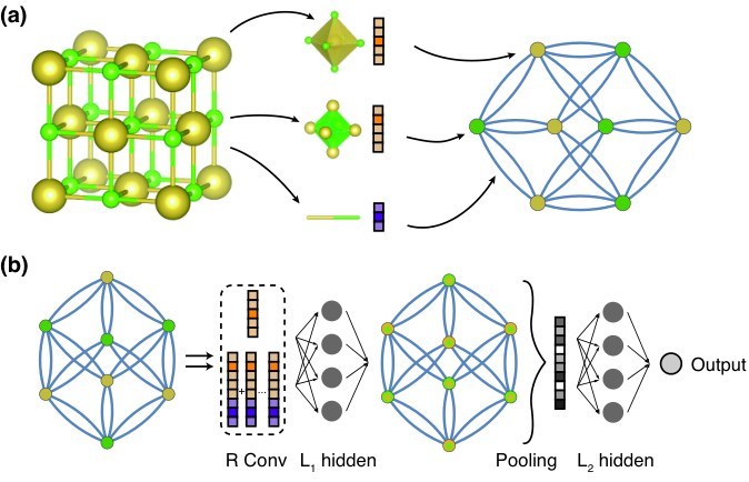
Figure 1: Illustration of the crystal graph convolutional neural network (CGCNN). (a) Construction of the crystal graph. Crystals are converted to graphs with nodes representing atoms in the unit cell and edges representing atom connections. Nodes and edges are characterized by vectors corresponding to the atoms and bonds in the crystal, respectively. (b) Structure of the convolutional neural network on top of the crystal graph. $R$ convolutional layers and $L_{1}$ hidden layers are built on top of each node, resulting in a new graph with each node representing the local environment of each atom. After pooling, a vector representing the entire crystal is connected to $L_{2}$ hidden layers, followed by the output layer to provide the prediction.

图 1：晶体图卷积网络（CGCNN）示意图。(a) 晶体图的构造。晶体被转换成图，节点表示晶胞中的原子，边表示原子之间的连接。节点和边分别用对应于晶体中原子和键的向量来刻画。(b) 建在晶体图之上的卷积网络结构。在每个节点上堆叠 $R$ 个卷积层和 $L_{1}$ 个隐层，得到一张新图，其中每个节点表示该原子的局域环境。池化之后，表示整个晶体的向量再接到 $L_{2}$ 个隐层，最后由输出层给出预测。

The main idea in our approach is to represent the crystal structure by a crystal graph that encodes both atomic information and bonding interactions between atoms, and then build a convolutional neural network on top of the graph to automatically extract representations that are optimum for predicting target properties by training with DFT calculated data. As illustrated in Figure 1 (a), a crystal graph $\mathcal{G}$ is an undirected multigraph which is defined by nodes representing atoms and edges representing connections between atoms in a crystal (the method for determining atom connectivity is explained in Supplemental Material[^1]). The crystal graph is unlike normal graphs since it allows multiple edges between the same pair of end nodes, a characteristic for crystal graphs due to their periodicity, in contrast to molecular graphs. Each node $i$ is represented by a feature vector $\bm{v}_{i}$, encoding the property of the atom corresponding to node $i$. Similarly, each edge $(i,j)_{k}$ is represented by a feature vector $\bm{u}_{(i,j)_{k}}$ corresponding to the $k$-th bond connecting atom $i$ and atom $j$.

我们方法的主要想法是：用一张同时编码原子信息和原子间成键相互作用的晶体图来表示晶体结构，然后在这张图上构建卷积网络，通过用 DFT 计算数据训练，自动抽出对预测目标性质最优的表示。如图 1(a) 所示，晶体图 $\mathcal{G}$ 是一个无向多重图，由表示原子的节点和表示晶体中原子连接的边定义（确定原子连通性的方法见补充材料[^1]）。与普通图不同，晶体图允许同一对端点之间有多条边，这是由周期性带来的、晶体图区别于分子图的一个特点。每个节点 $i$ 用特征向量 $\bm{v}_{i}$ 表示，编码对应于节点 $i$ 的原子性质。类似地，每条边 $(i,j)_{k}$ 用特征向量 $\bm{u}_{(i,j)_{k}}$ 表示，对应于连接原子 $i$ 和原子 $j$ 的第 $k$ 条键。

The convolutional neural networks built on top of the crystal graph consists of two major components: convolutional layers and pooling layers. Similar architectures have been used for computer vision[13], natural language processing[14], molecular fingerprinting[15], and general graph-structured data[16, 17] but not for crystal property prediction to the best of our knowledge. The convolutional layers iteratively update the atom feature vector $\bm{v}_{i}$ by “convolution” with surrounding atoms and bonds with a non-linear graph convolution function.

建在晶体图之上的卷积网络由两个主要部分组成：卷积层和池化层。类似的结构已被用于计算机视觉[13]、自然语言处理[14]、分子指纹[15]以及一般的图结构数据[16, 17]，但据我们所知，尚未用于晶体性质预测。卷积层通过与周围原子和键做“卷积”，用一个非线性的图卷积函数，迭代地更新原子特征向量 $\bm{v}_{i}$。

$$\bm{v}_{i}^{(t+1)}=\textrm{Conv}\left(\bm{v}_{i}^{(t)},\bm{v}_{j}^{(t)},\bm{u}_{(i,j)_{k}}\right),(i,j)_{k}\in\mathcal{G} \tag{1}$$

After $R$ convolutions, the network automatically learns the feature vector $\bm{v}_{i}^{(R)}$ for each atom by iteratively including its surrounding environment. The pooling layer is then used for producing an overall feature vector $\bm{v}_{c}$ for the crystal, which can be represented by a pooling function,

经过 $R$ 次卷积后，网络通过迭代地纳入周围环境，自动学到每个原子的特征向量 $\bm{v}_{i}^{(R)}$。随后用池化层产生整个晶体的总体特征向量 $\bm{v}_{c}$，它可以写成一个池化函数，

$$\bm{v_{c}}=\textrm{Pool}\left(\bm{v}_{0}^{(0)},\bm{v}_{1}^{(0)},...,\bm{v}_{N}^{(0)},...,\bm{v}_{N}^{(R)}\right) \tag{2}$$

that satisfies permutational invariance with respect to atom indexing and size invariance with respect to unit cell choice. In this work, a normalized summation is used as the pooling function for simplicity but other functions can also be used. In addition to the convolutional and pooling layers, two fully-connected hidden layers with the depth of $L_{1}$ and $L_{2}$ are added to capture the complex mapping between crystal structure and property. Finally, an output layer is used to connect the $L_{2}$ hidden layer to predict the target property $\hat{y}$.

该函数对原子编号满足置换不变，并对晶胞选取满足尺寸不变。本文为简单起见采用归一化求和作为池化函数，也可以使用其他函数。除了卷积层和池化层，我们还加入深度分别为 $L_{1}$ 和 $L_{2}$ 的两个全连接隐层，以刻画晶体结构与性质之间的复杂映射。最后，用一个输出层接到 $L_{2}$ 隐层，以预测目标性质 $\hat{y}$。

The training is performed by minimizing the difference between the predicted property $\hat{y}$ and the DFT calculated property $y$, defined by a cost function $J(y,\hat{y})$. The whole CGCNN can be considered as a function $f$ parameterized by weights $\bm{W}$ that maps a crystal $\mathcal{C}$ to the target property $\hat{y}$. Using backpropagation and stochastic gradient descent (SGD), we can solve the following optimization problem by iteratively updating the weights with DFT calculated data,

训练通过最小化预测性质 $\hat{y}$ 与 DFT 算出的性质 $y$ 之间的差异来完成，这一差异由代价函数 $J(y,\hat{y})$ 定义。整个 CGCNN 可以看成由权重 $\bm{W}$ 参数化的函数 $f$，它把晶体 $\mathcal{C}$ 映射到目标性质 $\hat{y}$。利用反向传播和随机梯度下降（SGD），我们可以通过用 DFT 计算数据迭代地更新权重，来求解下面的优化问题，

$$\displaystyle{\min_{\bm{W}}J(y,f(\mathcal{C};\bm{W}))} \tag{3}$$

the learned weights can then be used to predict material properties and provide chemical insights for future materials design.

学到的权重随后可以用来预测材料性质，并为未来的材料设计提供化学洞察。

In Supplemental Material (SM), we use a simple example to illustrate how a CGCNN composed of one linear convolution layer and one pooling layer can differentiate two crystal structures. With multiple convolution layers, pooling layers and hidden layers, CGCNN can extract any structure differences based on the atom connections and discover the underlaying relations between structure and property.

在补充材料（SM）中，我们用一个简单例子说明：只含一个线性卷积层和一个池化层的 CGCNN，如何区分两种晶体结构。在有多个卷积层、池化层和隐层时，CGCNN 可以根据原子连接抽出任何结构差异，并发现结构与性质之间的内在关系。

To demonstrate the generality of the CGCNN, we train the model using calculated properties from the Materials Project[11]. We focus on two types of generality in this work: (1) The structure types and chemical compositions for which our model can be applied, and (2) the number of properties that our model can accurately predict.

为了展示 CGCNN 的通用性，我们用 Materials Project[11] 中算出的性质来训练模型。本文关注两类通用性：（1）模型可以适用的结构类型和化学组成；（2）模型能够准确预测的性质数目。

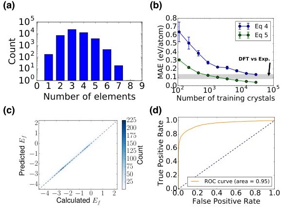
Figure 2: The performance of CGCNN on the Materials Project database[11]. (a) Histogram representing the distribution of the number of elements in each crystal. (b) Mean absolute error (MAE) as a function of training crystals for predicting formation energy per atom using different convolution functions. The shaded area denotes the MAE of DFT calculation compared with experiments[18]. (c) 2D histogram representing the predicted formation per atom against DFT calculated value. (d) Receiver operating characteristic (ROC) curve visualizing the result of metal-semiconductor classification. It plots the proportion of correctly identified metals (true positive rate) against the proportion of wrongly identified semiconductors (false positive rate) under different thresholds.

图 2：CGCNN 在 Materials Project 数据库[11]上的表现。(a) 表示每种晶体所含元素数目分布的直方图。(b) 用不同卷积函数预测每原子形成能时，平均绝对误差（MAE）随训练晶体数目的变化。阴影区表示 DFT 计算相对实验的 MAE[18]。(c) 表示预测的每原子形成能相对 DFT 计算值的二维直方图。(d) 可视化金属–半导体分类结果的受试者工作特征（ROC）曲线。它在不同阈值下，画出被正确识别为金属的比例（真阳性率）相对被错误识别为半导体的比例（假阳性率）。

The database we used includes a diverse set of inorganic crystals ranging from simple metals to complex minerals. After removing ill-converged crystals, the full database has 46744 materials covering 87 elements, 7 lattice systems and 216 space groups. As shown in Figure 2(a), the materials consist of as many as seven different elements, with 90% of them binary, ternary and quaternary compounds. The number of atoms in the primitive cell ranges from 1 to 200, and 90% of crystals have less than 60 atoms(Figure S2). Considering most of the crystals originate from the Inorganic Crystal Structure Database (ICSD)[19], this database is a good representation of known stoichiometric inorganic crystals.

我们使用的数据库包含从简单金属到复杂矿物的多种无机晶体。去掉收敛不好的晶体后，整个数据库有 46744 种材料，覆盖 87 种元素、7 种晶系和 216 个空间群。如图 2(a) 所示，这些材料最多可含七种不同元素，其中 90% 是二元、三元和四元化合物。原胞中的原子数从 1 到 200，90% 的晶体少于 60 个原子（图 S2）。考虑到其中大多数晶体来自无机晶体结构数据库（ICSD）[19]，这一数据库是已知化学计量无机晶体的良好代表。

The CGCNN is a flexible framework that allows variance in the crystal graph representation, neural network architecture, and training process, resulting in different $f$ in Eq. 3 and prediction performance. To choose the best model, we apply a train-validation scheme to optimize the prediction of formation energies of crystals. Each model is trained with 60% of the data and then validated with 20% of the data, and the best-performing model in validation set is selected. In our study, we find that the neural network architecture, especially the form of convolution function in Eq. 1, has the largest impact on prediction performance. We start with a simple convolution function,

CGCNN 是一个灵活的框架，允许晶体图表示、神经网络结构和训练过程有所变化，从而在式 3 中得到不同的 $f$ 和不同的预测表现。为了选出最好的模型，我们采用训练–验证方案来优化晶体形成能的预测。每个模型用 60% 的数据训练，再用 20% 的数据验证，并选出在验证集上表现最好的模型。在本研究中，我们发现神经网络结构，尤其是式 1 中卷积函数的形式，对预测表现影响最大。我们从一种简单的卷积函数出发，

$$\bm{v}_{i}^{(t+1)}=g\left[\left(\sum_{j,k}{\bm{v}_{j}^{(t)}\oplus\bm{u}_{(i,j)_{k}}}\right)\bm{W}_{c}^{(t)}+\bm{v}_{i}^{(t)}\bm{W}_{s}^{(t)}+\bm{b}^{(t)}\right] \tag{4}$$

where $\oplus$ denotes concatenation of atom and bond feature vectors, $\bm{W}_{c}^{(t)}$, $\bm{W}_{s}^{(t)}$, $\bm{b}^{(t)}$ are the convolution weight matrix, self weight matrix, and bias of the $t$-th layer, respectively, and $g$ is the activation function for introducing non-linear coupling between layers. By optimizing hyperparameters in Table S1, the lowest mean absolute error (MAE) for the validation set is 0.108 eV/atom. One limitation of Eq. 4 is that it uses a shared weight matrix $\bm{W}_{c}^{(t)}$ for all neighbors of $i$, which neglects the differences of interaction strength between neighbors. To overcome this problem, we design a new convolution function that first concatenates neighbor vectors $\bm{z}_{(i,j)_{k}}^{(t)}=\bm{v}_{i}^{(t)}\oplus\bm{v}_{j}^{(t)}\oplus\bm{u}_{(i,j)_{k}}$, then perform convolution by,

其中 $\oplus$ 表示原子和键特征向量的拼接，$\bm{W}_{c}^{(t)}$、$\bm{W}_{s}^{(t)}$、$\bm{b}^{(t)}$ 分别是第 $t$ 层的卷积权重矩阵、自身权重矩阵和偏置，$g$ 是用于在层之间引入非线性耦合的激活函数。通过优化表 S1 中的超参数，验证集上最低的平均绝对误差（MAE）为 0.108 eV/atom。式 4 的一个局限是，它对 $i$ 的所有近邻使用共享的权重矩阵 $\bm{W}_{c}^{(t)}$，从而忽略了近邻之间相互作用强度的差异。为了克服这个问题，我们设计了一种新的卷积函数：先把近邻向量拼接成 $\bm{z}_{(i,j)_{k}}^{(t)}=\bm{v}_{i}^{(t)}\oplus\bm{v}_{j}^{(t)}\oplus\bm{u}_{(i,j)_{k}}$，再按下面的方式做卷积，

$$\small\bm{v}_{i}^{(t+1)}=\bm{v}_{i}^{(t)}+\sum_{j,k}\sigma(\bm{z}_{(i,j)_{k}}^{(t)}\bm{W}_{f}^{(t)}+\bm{b}_{f}^{(t)})\odot g(\bm{z}_{(i,j)_{k}}^{(t)}\bm{W}_{s}^{(t)}+\bm{b}_{s}^{(t)}) \tag{5}$$

where $\odot$ denotes element-wise multiplication and $\sigma$ denotes a sigmoid function. In Eq. 5, the $\sigma(\bm{\cdot})$ functions as a learned weight matrix to differentiate interactions between neighbors, and adding $\bm{v}_{i}^{(t)}$ makes learning deeper networks easier[20]. We achieve MAE on the validation set of 0.039 eV/atom using the modified convolution function, a significant improvement compared to Eq. 4. In Figure S3, we compare the effects of several other hyperparameters on the MAE which are much smaller than the effect of convolution function.

其中 $\odot$ 表示逐元素乘法，$\sigma$ 表示 sigmoid 函数。在式 5 中，$\sigma(\bm{\cdot})$ 起着学得的权重矩阵的作用，用来区分近邻之间的相互作用；再加上 $\bm{v}_{i}^{(t)}$，使学习更深的网络变得更容易[20]。用修改后的卷积函数，我们在验证集上达到 0.039 eV/atom 的 MAE，相对式 4 有显著提高。在图 S3 中，我们比较了若干其他超参数对 MAE 的影响，它们都远小于卷积函数的影响。

Figure 2(b)(c) shows the performance of the two models on 9350 test crystals for predicting the formation energy per atom. We find a systematic decrease of the mean absolute error (MAE) of the predicted values compared with DFT calculated values for both convolution functions as the number of training data is increased. The best MAE’s we achieved with Eq. 4 and Eq. 5 are 0.136 eV/atom and 0.039 eV/atom, and 90% of the crystals are predicted within 0.3 eV/atom and 0.08 eV/atom errors, respectively. In comparison, Kirklin et al. reports that the MAE of DFT calculation with respect to experimental measurements in the Open Quantum Materials Database (OQMD) is 0.081–0.136 eV/atom depending on whether the energies of the elemental reference states are fitted, although they also find a large MAE of 0.082 eV/atom between different sources of experimental data. Given the comparison, our CGCNN approach provides a reliable estimation of DFT calculations and can potentially be applied to predict properties calculated by more accurate methods like GW[21] and quantum Monte Carlo[22].

图 2(b)(c) 给出了两个模型在 9350 个测试晶体上预测每原子形成能的表现。我们发现，对两种卷积函数，随着训练数据增多，预测值相对 DFT 计算值的平均绝对误差（MAE）都会系统地下降。用式 4 和式 5 达到的最好 MAE 分别为 0.136 eV/atom 和 0.039 eV/atom，并且分别有 90% 的晶体预测误差在 0.3 eV/atom 和 0.08 eV/atom 以内。作为对照，Kirklin 等人报告，在开放量子材料数据库（OQMD）中，DFT 计算相对实验测量的 MAE 为 0.081–0.136 eV/atom，具体取决于是否拟合元素参考态的能量；不过他们也发现，不同来源的实验数据之间仍有 0.082 eV/atom 的较大 MAE。由此看来，我们的 CGCNN 方法能够可靠地估计 DFT 计算结果，并有可能被用来预测由更精确的方法（如 GW[21] 和量子蒙特卡罗[22]）算出的性质。

Property	# of train data	Unit	$\textrm{MAE}_{\textrm{model}}$	$\textrm{MAE}_{\textrm{DFT}}$
Formation energy	28046	eV/atom	0.039	0.081–0.136[18]
Absolute energy	28046	eV/atom	0.072	–
Band gap	16458	eV	0.388	0.6[23]
Fermi energy	28046	eV	0.363	–
Bulk moduli	2041	log(GPa)	0.054	0.050[24]
Shear moduli	2041	log(GPa)	0.087	0.069[24]
Poisson ratio	2041	–	0.030	–

Table 1: Summary of the prediction performance of seven different properties on test sets.

性质	训练数据量	单位	$\textrm{MAE}_{\textrm{model}}$	$\textrm{MAE}_{\textrm{DFT}}$
形成能	28046	eV/atom	0.039	0.081–0.136[18]
绝对能量	28046	eV/atom	0.072	–
能隙	16458	eV	0.388	0.6[23]
费米能	28046	eV	0.363	–
体模量	2041	log(GPa)	0.054	0.050[24]
剪切模量	2041	log(GPa)	0.087	0.069[24]
泊松比	2041	–	0.030	–

表 1：七种不同性质在测试集上的预测表现汇总。

After establishing the generality of CGCNN with respect to the diversity of crystals, we next explore its prediction performance for different material properties. We apply the same framework to predict the absolute energy, band gap, Fermi energy, bulk moduli, shear moduli, and Poisson ratio of crystals using DFT calculated data from the Materials Project[11]. The prediction performance of Eq. 5 is improved compared to Eq. 4 for all six properties (Table S4). We summarize the performance in Table 1 and the corresponding 2D histograms in Figure S4. As we can see, the MAE of our model are close to or higher than DFT accuracy relative to experiments for most properties when ${\sim}10^{4}$ training data is used. For elastic properties, the errors are higher since less data is available, and the accuracy of DFT relative to experiments can be expected if ${\sim}10^{4}$ training data is available (Figure S5).

在确立了 CGCNN 相对晶体多样性的通用性之后，我们接下来考察它对不同材料性质的预测表现。我们用同一套框架，利用 Materials Project[11] 中的 DFT 计算数据，预测晶体的绝对能量、能隙、费米能、体模量、剪切模量和泊松比。对全部六种性质，式 5 的预测表现都优于式 4（表 S4）。我们把结果汇总于表 1，相应的二维直方图见图 S4。可以看到，当使用约 $10^{4}$ 个训练数据时，对大多数性质，模型的 MAE 已经接近或高于 DFT 相对实验的精度。对弹性性质，由于可用数据较少，误差更高；如果有约 $10^{4}$ 个训练数据，可以预期达到 DFT 相对实验的精度（图 S5）。

Recently, Jong et al.[25] developed a statistical learning (SL) framework using multivariate local regression on crystal descriptors to predict elastic properties using the same data from the Materials Project. By using the same number of training data, our model achieves root mean squared error (RMSE) on test sets of 0.105 log(GPa) and 0.127 log(GPa) for the bulk and shear moduli, which is similar to the RMSE of SL on the entire dataset of 0.0750 log(GPa) and 0.1378 log(GPa). Comparing the two methods, CGCNN predicts properties by extracting features only from crystal structure, while SL depends on crystal descriptors like cohesive energy and volume per atom. Recently, 1585 new crystals with elastic properties have been uploaded to the Materials Project database. Our model in Table 1 achieves MAE of 0.077 Log(GPa) for bulk moduli and 0.114 Log(GPa) for shear moduli on these crystals, showing good generalization to materials from potentially different crystal groups.

最近，Jong 等人[25]发展了一种统计学习（SL）框架，在晶体描述符上做多元局部回归，并用同一套来自 Materials Project 的数据预测弹性性质。在使用相同数量训练数据时，我们的模型在测试集上对体模量和剪切模量的均方根误差（RMSE）分别为 0.105 log(GPa) 和 0.127 log(GPa)，与 SL 在整个数据集上的 0.0750 log(GPa) 和 0.1378 log(GPa) 相近。比较这两种方法：CGCNN 只从晶体结构中抽取特征来预测性质，而 SL 依赖于内聚能、每原子体积这类晶体描述符。最近，又有 1585 种带弹性性质的新晶体被上传到 Materials Project 数据库。表 1 中的模型在这些晶体上对体模量和剪切模量的 MAE 分别为 0.077 Log(GPa) 和 0.114 Log(GPa)，表明模型对可能来自不同晶族的材料有良好的推广能力。

In addition to predicting continuous properties, CGCNN can also predict discrete properties by changing the output layer. By using a softmax activation function for the output layer and a cross entropy cost function, we can predict the classification of metal and semiconductor with the same framework. In Figure 2(d), we show the receiver operating characteristic (ROC) curve of the prediction on 9350 test crystals. Excellent prediction performance is achieved with the area under the curve (AUC) at 0.95. By choosing a threshold of 0.5, we get metal prediction accuracy at 0.80, semiconductor prediction accuracy at 0.95, and overall prediction accuracy at 0.90.

除了预测连续性质，只需改变输出层，CGCNN 也可以预测离散性质。通过给输出层使用 softmax 激活函数，并采用交叉熵代价函数，我们可以用同一套框架做金属与半导体的分类。图 2(d) 给出了在 9350 个测试晶体上预测的受试者工作特征（ROC）曲线。预测表现很好，曲线下面积（AUC）为 0.95。取阈值为 0.5 时，金属预测准确率为 0.80，半导体预测准确率为 0.95，总体预测准确率为 0.90。

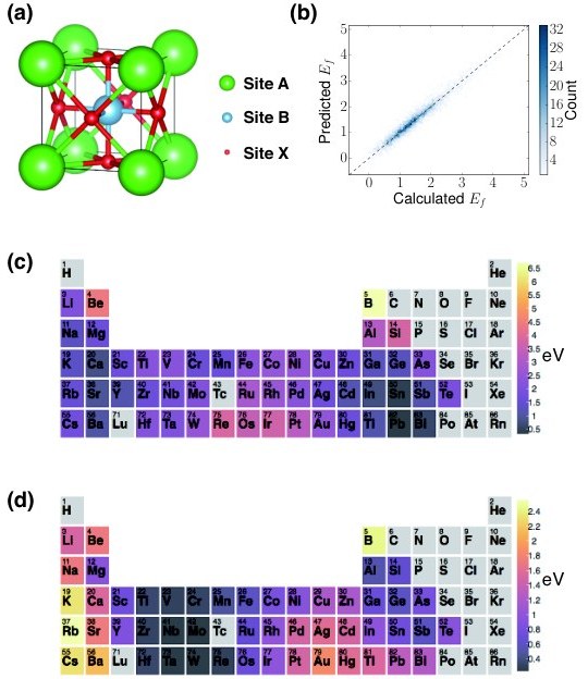
Figure 3: Extraction of site energy of perovskites from total energy above hull. (a) Structure of perovskites. (b) 2D histogram representing the predicted total formation against DFT calculated value. (c, d) Periodic table with the color of each element representing the mean of the site energy when the element occupies A site (c) or B site (d).

图 3：从总的能量高于凸包中抽出钙钛矿的格点能量。(a) 钙钛矿的结构。(b) 表示预测的总形成能相对 DFT 计算值的二维直方图。(c, d) 周期表，每种元素的颜色表示该元素占据 A 位 (c) 或 B 位 (d) 时格点能量的平均值。

Model interpretability is a desired property for any ML algorithms applied in materials science, because it can provide additional information for material design which may be more valuable than simply screening a large number of materials. However, non-linear functions are needed to learn the complex structure-property relations, resulting in ML models that are hard to interpret. CGCNN resolves this dilemma by separating the convolution and pooling layers. After the $R$ convolutional and $L_{1}$ hidden layers, we map the last atom feature vector $\bm{v}_{i}^{(R)}$ to a scalar $\tilde{v}_{i}$ and perform a linear pooling to predict the target property directly without the $L_{2}$ hidden layers (details discussed in SM). Therefore, we can learn the contribution of different local chemical environments, represented by $\tilde{v}_{i}$ for each atom, to the target property while maintaining a model with high capacity to ensure the prediction performance.

对任何用于材料科学的机器学习算法，模型可解释性都是一种被期望的性质，因为它可以为材料设计提供额外信息，而这些信息可能比仅仅筛选大量材料更有价值。然而，要学习复杂的结构–性质关系需要非线性函数，这又会使模型难以解释。CGCNN 通过把卷积层和池化层分开来解决这一两难。在 $R$ 个卷积层和 $L_{1}$ 个隐层之后，我们把最后的原子特征向量 $\bm{v}_{i}^{(R)}$ 映射成标量 $\tilde{v}_{i}$，再做线性池化，直接预测目标性质，而不再使用 $L_{2}$ 隐层（细节在补充材料中讨论）。这样，我们既能学习不同局域化学环境（由每个原子的 $\tilde{v}_{i}$ 表示）对目标性质的贡献，又能保持一个容量足够大的模型，以保证预测表现。

We demonstrate how these local chemical environment related information can be used to provide chemical insights and guide the material design by a specific example: learning the energy of each site in perovskites from the total energy above hull data. Perovskite is a crystal structure type with the form of $\text{ABX}{\vphantom{\text{X}}}_{\smash[t]{\text{3}}}$, where the site A atom sits at a corner position, the site B atom sits at a body centered position and site X atoms sit at face centered positions (Figure 3(a)). The database[26] we use includes the energy above hull of 18928 perovskite crystals, in which A and B sites can be any non-radioactive metals and X sites can be one or several elements from O, N, S, and F. We use the CGCNN with a linear pooling to predict the total energy above hull of perovskites in the database, using Eq. 4 as the convolution function. The resulting MAE on 3787 test perovskites is 0.130 eV/atom as shown in Figure 3(b), which is slightly higher than using a complete pooling layer and $L_{2}$ hidden layers (0.099 eV/atom as shown in Figure S6) due to the additional constraints introduced by the simplified pooling layer. However, this CGCNN allows us to learn the energy of each site in the crystal while training with the total energy above hull, providing additional insights for material design.

我们用一个具体例子说明，这些与局域化学环境有关的信息如何用来提供化学洞察并指导材料设计：从总的能量高于凸包数据中，学习钙钛矿中每个格点的能量。钙钛矿是一类化学式为 $\text{ABX}{\vphantom{\text{X}}}_{\smash[t]{\text{3}}}$ 的晶体结构，其中 A 位原子位于顶角，B 位原子位于体心，X 位原子位于面心（图 3(a)）。我们使用的数据库[26]包含 18928 个钙钛矿晶体的能量高于凸包，其中 A、B 位可以是任意非放射性金属，X 位可以是 O、N、S、F 中的一种或几种元素。我们使用带线性池化的 CGCNN，以式 4 作为卷积函数，预测数据库中钙钛矿总的能量高于凸包。如图 3(b) 所示，在 3787 个测试钙钛矿上得到的 MAE 为 0.130 eV/atom，略高于使用完整池化层和 $L_{2}$ 隐层时的 0.099 eV/atom（图 S6），这是因为简化的池化层引入了额外约束。不过，这一 CGCNN 使我们能够在用总的能量高于凸包训练的同时，学到晶体中每个格点的能量，从而为材料设计提供额外洞察。

Figure 3(c, d) visualizes the mean of the predicted site energies when each element occupies the A and B site respectively. The most stable elements that occupy the A site are those with large radii due to the space needed for 12 coordinations. In contrast, elements with small radii like Be, B, Si are the most unstable for occupying the A site. For the B site, elements in groups 4, 5, and 6 are the most stable throughout the periodic table. This can be explained by crystal field theory, since the configuration of d electrons of these elements favors the octahedral coordination in the B site. Interestingly, the visualization shows that large atoms from groups 13-15 are stable in the A site, in addition to the well-known region of groups 1-3 elements. Inspired by this result, we applied a combinational search for stable perovskites using elements from group 13-15 as the A site and group 4-6 as the B site. Due to the theoretical inaccuracies of DFT calculations and the possibility of metastable phases that can be stabilized by temperature, defects, and substrates, many synthesizable inorganic crystals have positive calculated energies above hull at $0\text{\,}\mathrm{K}$. Some metastable nitrides can even have energies up to 0.2 eV/atom above hull as a result of the strong bonding interactions[27]. In this work, since some of the perovskites are also nitrides, we choose to set the cutoff energy for potential synthesizability at $0.2\text{\,}\mathrm{e}\mathrm{V}\mathrm{/}\mathrm{a}\mathrm{t}\mathrm{o}\mathrm{m}$. We discovered 33 perovskites that fall within this threshold out of 378 in the entire dataset, among which 8 are within the cutoff out of 58 in the test set (Table S5). Many of these compounds like $\text{PbTiO}{\vphantom{\text{X}}}_{\smash[t]{\text{3}}}$[28], $\text{PbZrO}{\vphantom{\text{X}}}_{\smash[t]{\text{3}}}$[28], $\text{SnTaO}{\vphantom{\text{X}}}_{\smash[t]{\text{3}}}$[29], and $\text{PbMoO}{\vphantom{\text{X}}}_{\smash[t]{\text{3}}}$[30] have been experimentally synthesized. Note that $\text{PbMoO}{\vphantom{\text{X}}}_{\smash[t]{\text{3}}}$ has calculated energy 0.18 eV/atom above hull, indicating that our choice of cutoff energy is reasonable. In general, chemical insights gained from CGCNN can significantly reduce the search space for high throughput screening. In comparison, there are only 228 potentially synthesizable perovskites out of 18928 in our database: the chemical insight increased the search efficiency by a factor of 7.

图 3(c, d) 可视化了每种元素分别占据 A 位和 B 位时，预测格点能量的平均值。占据 A 位最稳定的，是那些半径较大的元素，因为 12 配位需要足够的空间。相反，Be、B、Si 这类半径很小的元素占据 A 位最不稳定。对 B 位，整个周期表中最稳定的是第 4、5、6 族元素。这可以用晶体场理论来解释，因为这些元素的 d 电子组态有利于 B 位上的八面体配位。有意思的是，可视化还显示，除了为人熟知的第 1–3 族元素区域外，第 13–15 族中的大原子在 A 位上也是稳定的。受这一结果启发，我们用第 13–15 族元素作为 A 位、第 4–6 族元素作为 B 位，做了稳定钙钛矿的组合搜索。由于 DFT 计算在理论上的偏差，以及亚稳相可能被温度、缺陷和衬底稳定下来，许多可合成的无机晶体在 $0\text{\,}\mathrm{K}$ 下算出的能量高于凸包为正。一些亚稳氮化物甚至可以高达 0.2 eV/atom，这是强成键相互作用的结果[27]。在本工作中，由于部分钙钛矿也是氮化物，我们把潜在可合成性的截止能量设为 $0.2\text{\,}\mathrm{e}\mathrm{V}\mathrm{/}\mathrm{a}\mathrm{t}\mathrm{o}\mathrm{m}$。在整个数据集的 378 个组合中，我们发现 33 个钙钛矿落在这一阈值内，其中测试集 58 个里有 8 个（表 S5）。其中许多化合物，如 $\text{PbTiO}{\vphantom{\text{X}}}_{\smash[t]{\text{3}}}$[28]、$\text{PbZrO}{\vphantom{\text{X}}}_{\smash[t]{\text{3}}}$[28]、$\text{SnTaO}{\vphantom{\text{X}}}_{\smash[t]{\text{3}}}$[29] 和 $\text{PbMoO}{\vphantom{\text{X}}}_{\smash[t]{\text{3}}}$[30]，已经被实验合成。需要指出的是，$\text{PbMoO}{\vphantom{\text{X}}}_{\smash[t]{\text{3}}}$ 算出的能量高于凸包为 0.18 eV/atom，说明我们选择的截止能量是合理的。总的来说，从 CGCNN 得到的化学洞察可以显著缩小高通量筛选的搜索空间。作为对照，我们数据库中 18928 个钙钛矿里只有 228 个具有潜在可合成性：化学洞察把搜索效率提高了 7 倍。

In summary, the crystal graph convolutional neural networks (CGCNN) presents a flexible machine learning framework for material property prediction and design knowledge extraction. The framework provides a reliable estimation of DFT calculations using around $10^{4}$ training data for 8 properties of inorganic crystals with diverse structure types and compositions. As an example of knowledge extraction, we apply this approach to the design of new perovskite materials and show that information extracted from the model is consistent with common chemical insights and significantly reduces the search space for high throughput screening.

总之，晶体图卷积网络（CGCNN）提供了一个灵活的机器学习框架，既可用于材料性质预测，也可用于提取设计知识。该框架用大约 $10^{4}$ 个训练数据，就能对结构类型和化学组成多样的无机晶体的 8 种性质，给出 DFT 计算的可靠估计。作为知识提取的一个例子，我们把这一方法用于新钙钛矿材料的设计，并表明从模型中抽出的信息与常见化学洞察一致，且能显著缩小高通量筛选的搜索空间。

The code for the CGCNN is available from Ref. [^2].

CGCNN 的代码见文献 [^2]。

Footnotes

脚注

1. See Supplemental Material for further details, including Refs. [32, 33, 34, 35, 36, 37, 38, 24, 4, 39].

1. 更多细节见补充材料，其中包括文献 [32, 33, 34, 35, 36, 37, 38, 24, 4, 39]。

2. CGCNN website: https://github.com/txie-93/cgcnn

2. CGCNN 网站：https://github.com/txie-93/cgcnn

3. The hidden layers $L_{1}$ and $L_{2}$ are not used simultaneously in this work. We only use $L_{2}$ for the prediction of material properties and $L_{1}$ for the learning of individual site energies in perovskites.

3. 本工作中隐层 $L_{1}$ 和 $L_{2}$ 不同时使用。我们只用 $L_{2}$ 预测材料性质，用 $L_{1}$ 学习钙钛矿中各个格点的能量。

4. $L^{2}$ regularization term $\lambda\left\|\bm{W}\right\|^{2}_{2}$ is added to cost function to reduce overfitting.

4. 在代价函数中加入 $L^{2}$ 正则项 $\lambda\left\|\bm{W}\right\|^{2}_{2}$，以减轻过拟合。

5. The lanthanide and actinide elements are considered as period 8 and 9 respectively.

5. 镧系和锕系元素分别视为第 8 周期和第 9 周期。

6. Log scale is used for these properties.

6. 这些性质使用对数标度。

References

参考文献

Acknowledgements.

This work was supported by Toyota Research Institute. Computational support was provided through the National Energy Research Scientific Computing Center, a DOE Office of Science User Facility supported by the Office of Science of the U.S. Department of Energy under Contract No. DE-AC02-05CH11231, and the Extreme Science and Engineering Discovery Environment, supported by National Science Foundation grant number ACI-1053575.

致谢。

本研究得到丰田研究所的资助。计算支持由国家能源研究科学计算中心提供，该中心是美国能源部科学办公室用户设施，由美国能源部科学办公室依据合同 DE-AC02-05CH11231 支持；以及极端科学与工程发现环境，该环境由美国国家科学基金会资助，资助号为 ACI-1053575。

[1] A. Seko, A. Togo, H. Hayashi, K. Tsuda, L. Chaput, and I. Tanaka, Physical review letters 115 , 205901 (2015).

[2] F. A. Faber, A. Lindmaa, O. A. von Lilienfeld, and R. Armiento, Physical Review Letters 117 , 135502 (2016).

[3] D. Xue, P. V. Balachandran, J. Hogden, J. Theiler, D. Xue, and T. Lookman, Nature communications 7 (2016).

[4] O. Isayev, C. Oses, C. Toher, E. Gossett, S. Curtarolo, and A. Tropsha, Nature Communications 8 (2017).

[5] L. M. Ghiringhelli, J. Vybiral, S. V. Levchenko, C. Draxl, and M. Scheffler, Physical review letters 114 , 105503 (2015).

[6] O. Isayev, D. Fourches, E. N. Muratov, C. Oses, K. Rasch, A. Tropsha, and S. Curtarolo, Chemistry of Materials 27 , 735 (2015).

[7] K. Schütt, H. Glawe, F. Brockherde, A. Sanna, K. Müller, and E. Gross, Physical Review B 89 , 205118 (2014).

[8] F. Faber, A. Lindmaa, O. A. von Lilienfeld, and R. Armiento, International Journal of Quantum Chemistry 115 , 1094 (2015).

[9] A. Seko, H. Hayashi, K. Nakayama, A. Takahashi, and I. Tanaka, Physical Review B 95 , 144110 (2017).

[10] Y. LeCun, Y. Bengio, and G. Hinton, Nature 521 , 436 (2015).

[11] A. Jain, S. P. Ong, G. Hautier, W. Chen, W. D. Richards, S. Dacek, S. Cholia, D. Gunter, D. Skinner, G. Ceder, et al. , Apl Materials 1 , 011002 (2013).

[12] See Supplemental Material for further details, including Refs.  [ 32 , 33 , 34 , 35 , 36 , 37 , 38 , 24 , 4 , 39 ] .

[13] A. Krizhevsky, I. Sutskever, and G. E. Hinton, in Advances in neural information processing systems (2012) pp. 1097–1105.

[14] R. Collobert and J. Weston, in Proceedings of the 25th international conference on Machine learning (ACM, 2008) pp. 160–167.

[15] D. K. Duvenaud, D. Maclaurin, J. Iparraguirre, R. Bombarell, T. Hirzel, A. Aspuru-Guzik, and R. P. Adams, in Advances in neural information processing systems (2015) pp. 2224–2232.

[16] M. Henaff, J. Bruna, and Y. LeCun, arXiv preprint arXiv:1506.05163 (2015).

[17] J. Gilmer, S. S. Schoenholz, P. F. Riley, O. Vinyals, and G. E. Dahl, in Proceedings of the 34th International Conference on Machine Learning, ICML 2017, Sydney, NSW, Australia, 6-11 August 2017 (2017) pp. 1263–1272.

[18] S. Kirklin, J. E. Saal, B. Meredig, A. Thompson, J. W. Doak, M. Aykol, S. Rühl, and C. Wolverton, npj Computational Materials 1 , 15010 (2015).

[19] M. Hellenbrandt, Crystallography Reviews 10 , 17 (2004).

[20] K. He, X. Zhang, S. Ren, and J. Sun, in Proceedings of the IEEE conference on computer vision and pattern recognition (2016) pp. 770–778.

[21] M. S. Hybertsen and S. G. Louie, Physical Review B 34 , 5390 (1986).

[22] W. Foulkes, L. Mitas, R. Needs, and G. Rajagopal, Reviews of Modern Physics 73 , 33 (2001).

[23] A. Jain, G. Hautier, C. J. Moore, S. P. Ong, C. C. Fischer, T. Mueller, K. A. Persson, and G. Ceder, Computational Materials Science 50 , 2295 (2011).

[24] M. De Jong, W. Chen, T. Angsten, A. Jain, R. Notestine, A. Gamst, M. Sluiter, C. K. Ande, S. Van Der Zwaag, J. J. Plata, et al. , Scientific data 2 , 150009 (2015).

[25] M. De Jong, W. Chen, R. Notestine, K. Persson, G. Ceder, A. Jain, M. Asta, and A. Gamst, Scientific reports 6 (2016).

[26] I. E. Castelli, T. Olsen, S. Datta, D. D. Landis, S. Dahl, K. S. Thygesen, and K. W. Jacobsen, Energy & Environmental Science 5 , 5814 (2012).

[27] W. Sun, S. T. Dacek, S. P. Ong, G. Hautier, A. Jain, W. D. Richards, A. C. Gamst, K. A. Persson, and G. Ceder, Science Advances 2 , e1600225 (2016).

[28] G. Shirane, K. Suzuki, and A. Takeda, Journal of the Physical Society of Japan 7 , 12 (1952).

[29] J. Lang, C. Li, X. Wang, et al. , Materials Today: Proceedings 3 , 424 (2016).

[30] H. Takatsu, O. Hernandez, W. Yoshimune, C. Prestipino, T. Yamamoto, C. Tassel, Y. Kobayashi, D. Batuk, Y. Shibata, A. M. Abakumov, et al. , Physical Review B 95 , 155105 (2017).

[31] CGCNN website: https://github.com/txie-93/cgcnn .

[32] R. Sanderson, Science 114 , 670 (1951).

[33] R. Sanderson, Journal of the American Chemical Society 74 , 4792 (1952).

[34] B. Cordero, V. Gómez, A. E. Platero-Prats, M. Revés, J. Echeverría, E. Cremades, F. Barragán, and S. Alvarez, Dalton Transactions , 2832 (2008).

[35] A. Kramida, Y. Ralchenko, J. Reader, et al. , National Institute of Standards and Technology, Gaithersburg, MD (2013).

[36] W. M. Haynes, CRC handbook of chemistry and physics (CRC press, 2014).

[37] D. Kingma and J. Ba, arXiv preprint arXiv:1412.6980 (2014).

[38] N. Srivastava, G. E. Hinton, A. Krizhevsky, I. Sutskever, and R. Salakhutdinov, Journal of Machine Learning Research 15 , 1929 (2014).

[39] V. A. Blatov*, Crystallography reviews 10 , 249 (2004).

I Supplementary Methods and Discussions

I 补充方法与讨论

I.1 Construction of crystal graphs

I.1 晶体图的构造

The connectivity between atoms in a crystal graph is determined by a method inspired by Ref. [4]. For each atom, neighbors are first searched within $6\text{\,}\mathrm{\SIUnitSymbolAngstrom}$ radius, and they are considered as connected when they share a Voronoi face [39] with the center atom and have interatomic distance lower than the sum of the Cordero covalent bond lengths [34] with a $0.25\text{\,}\mathrm{\SIUnitSymbolAngstrom}$ tolerance. Therefore, only strong bonding interactions are considered in the crystal graph construction.

晶体图中原子之间的连通性，采用一种受文献 [4] 启发的方法来确定。对每个原子，先在 $6\text{\,}\mathrm{\SIUnitSymbolAngstrom}$ 半径内搜索近邻；当近邻与中心原子共用一个 Voronoi 面[39]，且原子间距小于 Cordero 共价键长之和[34]再加上 $0.25\text{\,}\mathrm{\SIUnitSymbolAngstrom}$ 容差时，即视为相连。因此，构造晶体图时只考虑较强的成键相互作用。

It is worth noting that by using convolution function Eq. 5 in the main text, the connectivity between atoms becomes less important because the $\sigma(\bm{\cdot})$ part automatically ignores weak bonds. In practice, we discover that connecting 12 nearest neighbors in the initial graph construction performs as good as using the method described above.

值得指出的是，若使用正文中的卷积函数式 5，原子连通性就不那么关键了，因为 $\sigma(\bm{\cdot})$ 部分会自动忽略弱键。实践中我们发现，在最初构图时把 12 个最近邻连上，表现与上述方法相当。

Atom and bond properties are encoded in node feature vectors $\bm{v}_{i}$ and edge feature vectors $\bm{u}_{(i,j)_{k}}$ using one hot encoding. For discrete values, the vectors are encoded according to the category that the value belongs to; for continuous values, the range of property values is evenly divided to 10 categories and the vectors are encoded accordingly. The full list of atom and bond properties as well as their ranges are in Table 2 and Table 3. For instance, if we use the group number and period number as atom features, the atom feature vector for H will be a 27-dimensional vector with 1st and 19th element being 1 and other elements being 0. If the interatomic distance is 0.7, then the bond feature vector will be a 10-dimensional vector with 1st element being 1 and other elements being 0.

原子和键的性质分别用独热编码写入节点特征向量 $\bm{v}_{i}$ 和边特征向量 $\bm{u}_{(i,j)_{k}}$。对离散取值，按该值所属类别编码；对连续取值，把取值范围均匀分成 10 类后再编码。原子和键性质的完整列表及其取值范围见表 2 和表 3。例如，若用族号和周期号作为原子特征，则 H 的原子特征向量是一个 27 维向量，第 1 个和第 19 个元素为 1，其余为 0。若原子间距为 0.7，则键特征向量是一个 10 维向量，第 1 个元素为 1，其余为 0。

I.2 Illustrative example for differentiating NaCl and KCl

I.2 区分 NaCl 与 KCl 的示意例子

We provide a simple illustrative example to explain how CGCNN works by completing the task of differentiating the structures of NaCl and KCl. Concretely, the task is to predict +1 if the crystal structure is NaCl and -1 if the structure is KCl. We can accomplish it with a CGCNN with only one convolutional layer and one pooling layer.

我们用一个简单的示意例子说明 CGCNN 如何工作：完成区分 NaCl 与 KCl 结构的任务。具体地说，若晶体结构是 NaCl，则预测 $+1$；若是 KCl，则预测 $-1$。只用一个卷积层和一个池化层的 CGCNN 就可以做到这一点。

In Fig. S1, we convert the original crystal structures of NaCl and KCl to their corresponding crystal graphs. Note that the four Na and Cl nodes in the crystal graph of NaCl all have the same chemical environments, and we can actually simplify it to a crystal graph with two nodes. Here we use this eight-node crystal graph to illustrate that CGCNN is invariant to the choice of unit cells. For simplicity, we only use atom feature vectors without bond feature vectors in crystal graphs, since it is enough to differentiate NaCl and KCl. Specifically, each node is represented by following vectors according to the element information.

在图 S1 中，我们把 NaCl 和 KCl 的原始晶体结构转换成对应的晶体图。需要注意的是，NaCl 晶体图中四个 Na 节点和四个 Cl 节点各自具有相同的化学环境，实际上可以简化成只有两个节点的晶体图。这里仍用这张八节点晶体图，是为了说明 CGCNN 对晶胞选取是不变的。为简单起见，晶体图里只使用原子特征向量、不使用键特征向量，因为这已足以区分 NaCl 和 KCl。具体地，每个节点按元素信息表示成如下向量。

$$\bm{v}_{\mathrm{Cl}}=\begin{pmatrix}1&0&0\end{pmatrix};\bm{v}_{\mathrm{Na}}=\begin{pmatrix}0&1&0\end{pmatrix};\bm{v}_{\mathrm{K}}=\begin{pmatrix}0&0&1\end{pmatrix}; \tag{S1}$$

Then, we apply one convolutions to each node in the two crystal graphs according to Eq. 4 in the main text. We initialize $\bm{W}_{c}$ and $\bm{W}_{s}$ as,

随后，按正文中的式 4，对两张晶体图中的每个节点做一次卷积。把 $\bm{W}_{c}$ 和 $\bm{W}_{s}$ 初始化为

$$\bm{W}{c}=\begin{pmatrix}w{c1}\
w_{c2}\
w_{c3}\end{pmatrix};\bm{W}{s}=\begin{pmatrix}w{s1}\
w_{s2}\
w_{s3}\end{pmatrix}; \tag{S2}$$

and for simplicity, we set $\bm{b}=\bm{0}$ and $g(x)=x$. After one convolution, in NaCl, the feature of each node becomes,

并且为简单起见，取 $\bm{b}=\bm{0}$、$g(x)=x$。经过一次卷积后，在 NaCl 中每个节点的特征变为

$$\displaystyle\bm{v}_{\mathrm{Na}}^{(1)} \\ \displaystyle=6w_{c1}+w_{s2} \\ \displaystyle\bm{v}_{\mathrm{Cl}}^{(1)} \\ \displaystyle=6w_{c2}+w_{s1} \tag{S3}$$

and in KCl,

而在 KCl 中为

$$\displaystyle\bm{v}_{\mathrm{K}}^{(1)} \\ \displaystyle=8w_{c1}+w_{s3} \\ \displaystyle\bm{v}_{\mathrm{Cl}}^{(1)} \\ \displaystyle=8w_{c3}+w_{s1} \tag{S5}$$

After convolution, we apply a simple normalized pooling by summing over the feature vectors of all nodes $\bm{v}_{i}^{(1)}$ within the crystal graph, and then divide it by the total number of nodes. Consequently, the overall feature vectors of the two crystal graphs are,

卷积之后，我们做一个简单的归一化池化：把晶体图内所有节点的特征向量 $\bm{v}_{i}^{(1)}$ 求和，再除以节点总数。于是，两张晶体图的总体特征向量为

$$\displaystyle\bm{v}_{\mathrm{NaCl}}=3w_{c1}+3w_{c2}+0.5w_{s1}+0.5w_{s2} \\ \displaystyle\bm{v}_{\mathrm{KCl}}=4w_{c1}+4w_{c3}+0.5w_{s1}+0.5w_{s3} \tag{S7}$$

Since the crystal feature vectors are already one-dimension, we do not need another output layer to map them into the target value. So, our predictions are,

由于晶体特征向量已经是一维的，不再需要额外的输出层把它们映射到目标值。因此，预测结果为

$$\displaystyle\hat{y}_{\mathrm{NaCl}}=3w_{c1}+3w_{c2}+0.5w_{s1}+0.5w_{s2} \\ \displaystyle\hat{y}_{\mathrm{KCl}}=4w_{c1}+4w_{c3}+0.5w_{s1}+0.5w_{s3} \tag{S9}$$

We can easily find $\bm{W}_{c}$ and $\bm{W}_{s}$ that make $\hat{y}_{\mathrm{NaCl}}=1$ and $\hat{y}_{\mathrm{KCl}}=-1$, showing that CGCNN are capable of differentiating NaCl and KCl. In this example, the existence of certain weights $w_{ci}$ or $w_{si}$ in Eq. S9 and Eq. S10 indicates the occurrence of elements as centers or neighbors respectively, while the factor represents the frequency of occurrence, both of which can help differentiating the two crystals.

我们不难找到一组 $\bm{W}_{c}$ 和 $\bm{W}_{s}$，使得 $\hat{y}_{\mathrm{NaCl}}=1$、$\hat{y}_{\mathrm{KCl}}=-1$，这说明 CGCNN 能够区分 NaCl 与 KCl。在这个例子里，式 S9 和式 S10 中某些权重 $w_{ci}$ 或 $w_{si}$ 是否出现，分别表示该元素作为中心或近邻是否出现；前面的系数则表示出现的频次。这两方面都可以帮助区分这两种晶体。

When more training data is available, we could not find $\bm{W}_{c}$ and $\bm{W}_{s}$ that result in zero loss since the weights are shared for all crystals. Methods like stochastic gradient descent (SGD) can me used to minimize the loss and find the weights that maximize the prediction performance. Also, more complex CGCNN structures can be used to capture more structure information.

当训练数据更多时，由于权重在所有晶体上是共享的，我们通常找不到使损失为零的 $\bm{W}_{c}$ 和 $\bm{W}_{s}$。可以用随机梯度下降（SGD）这类方法来最小化损失，并找到使预测表现最好的权重。也可以采用更复杂的 CGCNN 结构，以捕捉更多结构信息。

I.3 Hyperparameter optimization

I.3 超参数优化

The hyperparameters are parameters that defines the CGCNN. They include graph parameters that are used to generate the crystal graph, architecture parameters that are used to define the convolutional neural network on top of the crystal graph, and training parameters that are used for the training process. Unlike the weights that are trained via SGD, the hyperparameters are chosen through a train-validation process.

超参数是用来定义 CGCNN 的参数。它们包括：用于生成晶体图的图参数、用于定义晶体图上卷积网络的结构参数，以及用于训练过程的训练参数。与经 SGD 训练得到的权重不同，超参数通过训练–验证过程来选取。

We first randomly divide our database into three parts: training set (60%), validation set (20%), and test set (20%). Model with different hyperparameters are trained on training set via SGD, and the resulting weights are used to predict the property of crystals in validation set. By comparing to the properties calculated by DFT, and the hyperparameters that provide lowest MAE or AOC in the validation set are chosen as the optimum hyperparameters.

我们首先把数据库随机分成三部分：训练集（60%）、验证集（20%）和测试集（20%）。具有不同超参数的模型在训练集上用 SGD 训练，再用得到的权重去预测验证集中晶体的性质。把预测与 DFT 算出的性质比较后，在验证集上给出最低 MAE 或 AUC 的超参数，就被选为最优超参数。

For convolution function Eq. 4, we use random search to optimize all the hyperparameters listed in Table 1. Since the influence of hyperparameter optimization is much smaller than the convolution functions as shown in Fig. S3, we only optimize number of convolutional layers, regularization term, and step size of the Adam optimizer when using convolution function Eq. 5.

对卷积函数式 4，我们用随机搜索优化表 1 中列出的全部超参数。如图 S3 所示，超参数优化的影响远小于卷积函数的选择，因此在使用卷积函数式 5 时，我们只优化卷积层数、正则项，以及 Adam 优化器的步长。

I.4 Pooling layer choices

I.4 池化层的选择

Throughout this work, normalized summation is used as a pooling function as described in the main text. However, for convolutional function Eq. 4, we sum up different feature vectors for the purpose of either maximizing prediction performance or interpretability.

在整个工作中，池化函数采用正文所述的归一化求和。不过，对卷积函数式 4，我们会按不同目的对特征向量做不同的求和：一是为了尽量提高预测表现，一是为了可解释性。

To maximize prediction performance, we utilize feature vectors from all convolutional layers. Each feature vector $\bm{v}_{i}^{(t)}$ from the $t$-th convolution is first transformed to the same dimension by a linear map and then sparsified by a Softmax function (Eq. S12), resulting in a vector $\bm{\tilde{v}}_{i}^{(t)}$ with the same dimension. Then, the pooling layer sums over feature vectors $\bm{\tilde{v}}_{i}^{(t)}$ from all convolutional layers where $t=0,1,..,R$ and over all atoms $i=1,2,...,N$. The resulting crystal vector $\bm{v_{c}}$ is then normalized to be invariant to crystal size. This pooling includes all intermediate feature vectors representing chemical environments of various radius, which is more complete and resulting better prediction performance.

为尽量提高预测表现，我们利用来自全部卷积层的特征向量。第 $t$ 次卷积得到的每个特征向量 $\bm{v}_{i}^{(t)}$ 先经线性映射变到同一维数，再用 Softmax 函数（式 S12）稀疏化，得到同维的向量 $\bm{\tilde{v}}_{i}^{(t)}$。随后，池化层对所有卷积层 $t=0,1,\ldots,R$ 以及所有原子 $i=1,2,\ldots,N$ 的特征向量 $\bm{\tilde{v}}_{i}^{(t)}$ 求和。得到的晶体向量 $\bm{v_{c}}$ 再做归一化，使其对晶体尺寸不变。这种池化纳入了表示不同半径化学环境的全部中间特征向量，信息更完整，因而预测表现更好。

$$\textrm{Softmax}\left(\bm{z}\right)_{j}=\frac{\exp(z_{j})}{\sum_{k}\exp(z_{k})} \tag{S11}$$

$$\bm{\tilde{v}}_{i}^{(t)}=\textrm{Softmax}(\bm{W}_{t}\bm{v}_{i}^{(t)}+\bm{b}_{t}) \tag{S12}$$

$$\bm{v_{c}}=\sum_{t,i}\bm{\tilde{v}}_{i}^{(t)} \tag{S13}$$

To get better interpretability, we directly map the final feature vector after $R$ convolutional layers and $L_{1}$ hidden layers $\bm{v}_{i}^{(R)}$ to a scalar $\tilde{v}_{i}$ using a linear transform (Eq. S14), and then summing up the scalars to predict the target property $v_{c}$. After training with the global property $v_{c}$, the model automatically learns the contribution of each local chemical environments represented by $\tilde{v}_{i}$.

为获得更好的可解释性，我们把经过 $R$ 个卷积层和 $L_{1}$ 个隐层后的最终特征向量 $\bm{v}_{i}^{(R)}$，用线性变换（式 S14）直接映射成标量 $\tilde{v}_{i}$，再对这些标量求和，以预测目标性质 $v_{c}$。在用全局性质 $v_{c}$ 训练之后，模型会自动学到由 $\tilde{v}_{i}$ 表示的各局域化学环境的贡献。

$$\tilde{v}_{i}=\bm{W}^{T}\bm{v}_{i}^{(R)}+b \tag{S14}$$

$$v_{c}=\frac{1}{N}\sum_{i}\tilde{v}_{i} \tag{S15}$$

For convolution function Eq. 5, we directly compute the normalized sum of the last feature vector $\bm{v}_{i}^{(R)}$ after R convolutional layers as a pooling function (Eq. S16) since the residual structure in Eq. 5 allows information passed to the last layer which makes adding $\bm{v}_{i}^{(t)}$ from previous convolutional layers unnecessary.

对卷积函数式 5，我们直接把经过 $R$ 个卷积层后的最后特征向量 $\bm{v}_{i}^{(R)}$ 做归一化求和，作为池化函数（式 S16）。这是因为式 5 中的残差结构允许信息传到最后一层，因而没有必要再把前面各卷积层的 $\bm{v}_{i}^{(t)}$ 加进来。

$$\bm{v}_{c}=\frac{1}{N}\sum_{i}\bm{v}_{i}^{(R)} \tag{S16}$$

II Supplementary Figures

II 补充图

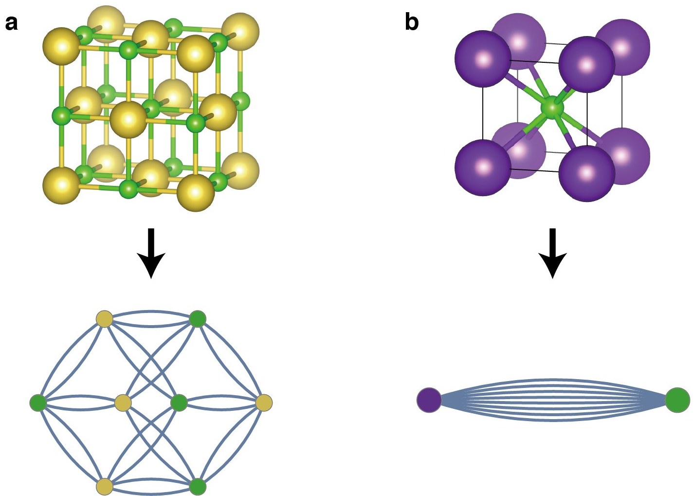
Figure S1: The crystal structures and crystal graphs of NaCl (a) and KCl (b).

图 S1：NaCl（a）和 KCl（b）的晶体结构与晶体图。

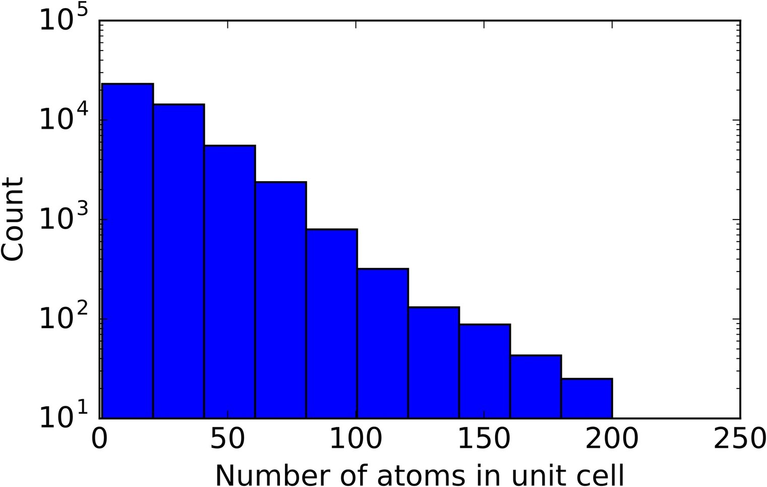
Figure S2: Histogram representing the distribution of the number of atoms in the primitive cells.

图 S2：表示原胞中原子数目分布的直方图。

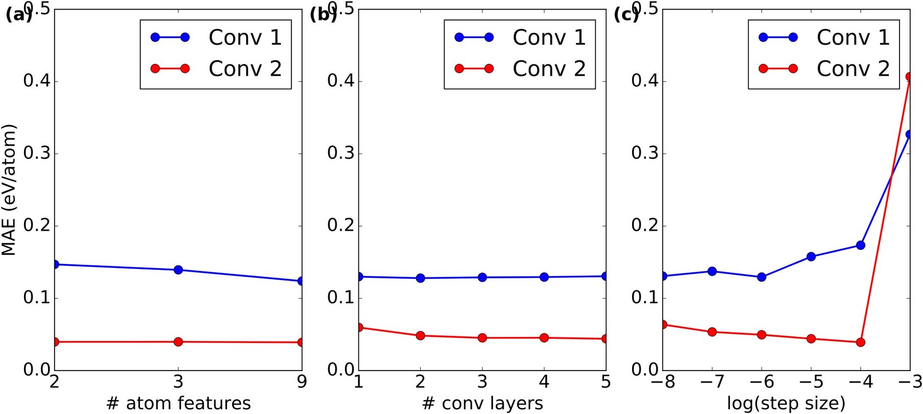
Figure S3: The effect of different hyperparameters on the validation mean absolute errors (MAEs). The blue points denotes models using convolution function Eq. 4, and the red points denotes models using Eq. 5. (a) Number of atom features. The 2 features include group number and period number, the 3 features additionally include electronegativity, and the 9 features include all properties in Table 2. (b) Number of convolutional layers. (c) Logarithm of the step size.

图 S3：不同超参数对验证集平均绝对误差（MAE）的影响。蓝点表示使用卷积函数式 4 的模型，红点表示使用式 5 的模型。(a) 原子特征数目。2 个特征包括族号和周期号；3 个特征再加入电负性；9 个特征包括表 2 中的全部性质。(b) 卷积层数。(c) 步长的对数。

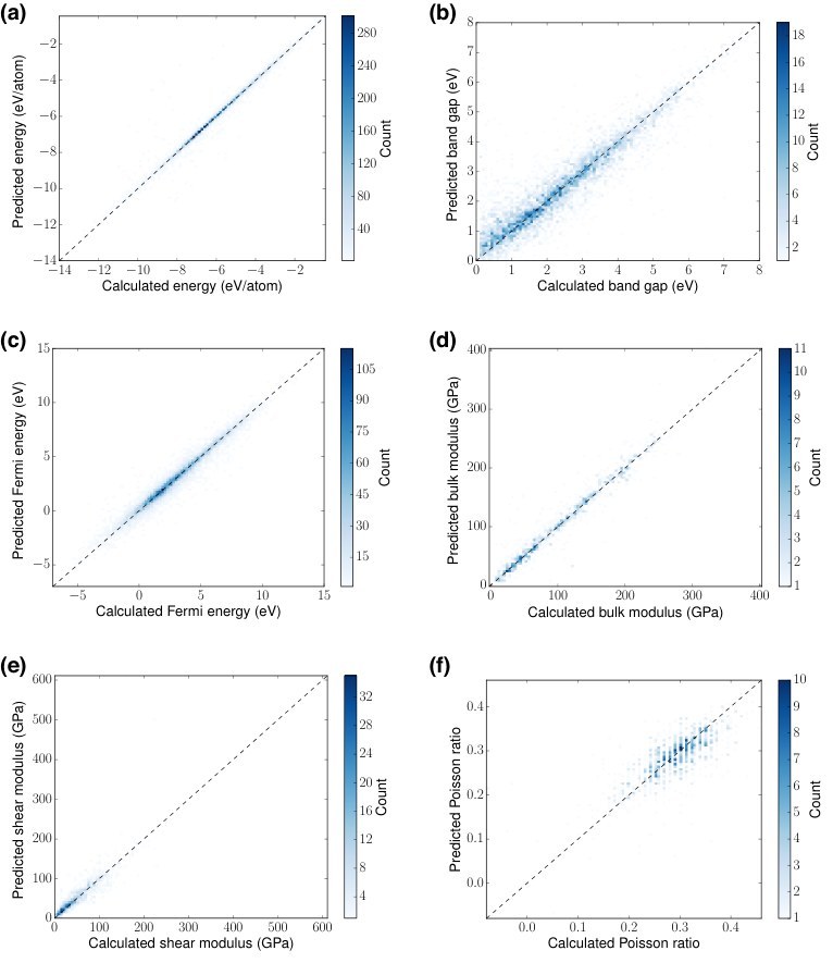
Figure S4: 2D histogram visualizing the predictive performance of six properties. (a) Total energy per atom. (b) Band gap. (c) Fermi energy. (d) Bulk moduli. (e) Shear moduli. (e) Poisson ratio.

图 S4：可视化六种性质预测表现的二维直方图。(a) 每原子总能量。(b) 能隙。(c) 费米能。(d) 体模量。(e) 剪切模量。(f) 泊松比。

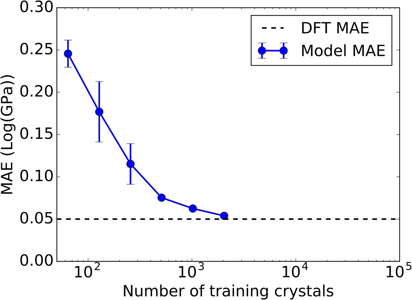
Figure S5: The MAE of predicted bulk modulus with respect to DFT values against the number of training crystals. The dashed line shows the MAE of DFT calculations with respect to experimental results [24], which is 0.050 Log(GPa).

图 S5：预测体模量相对 DFT 值的 MAE 随训练晶体数目的变化。虚线给出 DFT 计算相对实验结果的 MAE[24]，为 0.050 Log(GPa)。

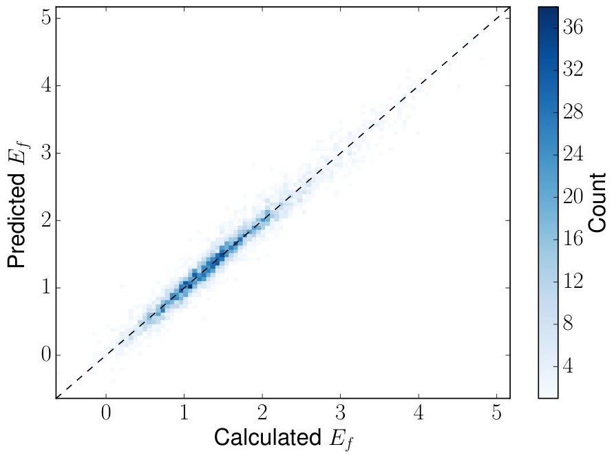
Figure S6: 2D histogram visualizing the performance of predicting formation energy of perovskites using a full pooling layer with Eq. 4 as the convolution function.

图 S6：用完整池化层、并以式 4 作为卷积函数时，预测钙钛矿形成能表现的二维直方图。

III Supplementary Tables

III 补充表

Hyperparameter	Range
Number of properties used in atom feature vector $\bm{v}_{i}$	2, 3, 10
Number of convolutional layers	1, 2, …, 5
Length of learned atom feature vector $\bm{v}_{i}^{(t)}$	10, 20, 50, 100, 200
Number of hidden layer $L_{1}$[^1]	1, 2, …, 4
Number of hidden layer $L_{2}$[^1]	1, 2, …, 5
Regularization term $\lambda$[^2]	$\mathrm{e}^{-6},\mathrm{e}^{-4}$, $\mathrm{e}^{-2}$, $\mathrm{e}^{0}$
Scaling factor of the Gaussian initialization of weights	$\mathrm{e}^{-8}$, $\mathrm{e}^{-6}$, $\mathrm{e}^{-4}$, $\mathrm{e}^{-2}$
Step size of the Adam optimizer[37]	$\mathrm{e}^{-8}$, $\mathrm{e}^{-7}$, $\mathrm{e}^{-6}$, $\mathrm{e}^{-5}$, $\mathrm{e}^{-4}$, $\mathrm{e}^{-3}$
Dropout fraction[38]	0, 0.1, 0.2

Table 1: A list of hyperparameters that are optimized in this work.

超参数	取值范围
原子特征向量 $\bm{v}_{i}$ 所用性质数目	2, 3, 10
卷积层数	1, 2, …, 5
学得的原子特征向量 $\bm{v}_{i}^{(t)}$ 的长度	10, 20, 50, 100, 200
隐层 $L_{1}$ 的层数[^1]	1, 2, …, 4
隐层 $L_{2}$ 的层数[^1]	1, 2, …, 5
正则项 $\lambda$[^2]	$\mathrm{e}^{-6},\mathrm{e}^{-4}$, $\mathrm{e}^{-2}$, $\mathrm{e}^{0}$
权重高斯初始化的缩放因子	$\mathrm{e}^{-8}$, $\mathrm{e}^{-6}$, $\mathrm{e}^{-4}$, $\mathrm{e}^{-2}$
Adam 优化器的步长[37]	$\mathrm{e}^{-8}$, $\mathrm{e}^{-7}$, $\mathrm{e}^{-6}$, $\mathrm{e}^{-5}$, $\mathrm{e}^{-4}$, $\mathrm{e}^{-3}$
Dropout 比例[38]	0, 0.1, 0.2

表 1：本工作中优化的超参数列表。

Property	Unit	Range	# of categories
Group number	–	1,2, …, 18	18
Period number	–	1,2, ..., 9[^1]	9
Electronegativity[32, 33]	–	0.5–4.0	10
Covalent radius[34]	pm	25–250	10
Valence electrons	–	1, 2, …, 12	12
First ionization energy[35][^2]	eV	1.3–3.3	10
Electron affinity[36]	eV	-3–3.7	10
Block	–	s, p, d, f	4
Atomic volume[^2]	$\text{\,}\mathrm{c}\mathrm{m}^{3}\mathrm{/}\mathrm{m}\mathrm{o}\mathrm{l}$	1.5–4.3	10

Table 2: Properties used in atom feature vector $\bm{v}_{i}$

性质	单位	取值范围	类别数
族号	–	1,2, …, 18	18
周期号	–	1,2, ..., 9[^1]	9
电负性[32, 33]	–	0.5–4.0	10
共价半径[34]	pm	25–250	10
价电子数	–	1, 2, …, 12	12
第一电离能[35][^2]	eV	1.3–3.3	10
电子亲和能[36]	eV	-3–3.7	10
区块	–	s, p, d, f	4
原子体积[^2]	$\text{\,}\mathrm{c}\mathrm{m}^{3}\mathrm{/}\mathrm{m}\mathrm{o}\mathrm{l}$	1.5–4.3	10

表 2：原子特征向量 $\bm{v}_{i}$ 所用的性质

Property	Unit	Range	# of categories
Atom distance	$\text{\,}\mathrm{\SIUnitSymbolAngstrom}$	0.7–5.2	10

Table 3: Properties used in bond feature vector $\bm{u}_{(i,j)_{k}}$

性质	单位	取值范围	类别数
原子间距	$\text{\,}\mathrm{\SIUnitSymbolAngstrom}$	0.7–5.2	10

表 3：键特征向量 $\bm{u}_{(i,j)_{k}}$ 所用的性质

Property	# Train data	Unit	$\textrm{MAE}_{\textrm{Eq.~4}}$	$\textrm{MAE}_{\textrm{Eq.~5}}$
Formation energy	28046	eV/atom	0.112	0.039
Absolute energy	28046	eV/atom	0.227	0.072
Band gap	16458	eV	0.530	0.388
Fermi energy	28046	eV	0.564	0.363
Bulk moduli	2041	Log(GPa)	0.084	0.054
Shear moduli	2041	Log(GPa)	0.113	0.087
Poisson ratio	2041	–	0.033	0.030

Table 4: Comparison of the prediction performance of seven different properties on test sets using different convolution functions.

性质	训练数据量	单位	$\textrm{MAE}_{\textrm{Eq.~4}}$	$\textrm{MAE}_{\textrm{Eq.~5}}$
形成能	28046	eV/atom	0.112	0.039
绝对能量	28046	eV/atom	0.227	0.072
能隙	16458	eV	0.530	0.388
费米能	28046	eV	0.564	0.363
体模量	2041	Log(GPa)	0.084	0.054
剪切模量	2041	Log(GPa)	0.113	0.087
泊松比	2041	–	0.033	0.030

表 4：使用不同卷积函数时，七种性质在测试集上的预测表现比较。

Formula	A site	B site	Formation energy per atom (eV/atom)
Training Set (60%)
TlNbO3	Tl	Nb	0.0
SnTiO3	Sn	Ti	0.1
PbVO3	Pb	V	0.04
SnTaO3	Sn	Ta	0.0
TlWO3	Tl	W	0.12
PbMoO3	Pb	Mo	0.18
PbCrO3	Pb	Cr	0.14
SnNbO3	Sn	Nb	0.14
SnTaO2N	Sn	Ta	0.14
TlTaOFN	Tl	Ta	0.18
TlTaO2F	Tl	Ta	0.04
TlHfO2F	Tl	Hf	0.18
PbTiO3	Pb	Ti	0.06
InNbO3	In	Nb	0.06
InWO3	In	W	0.18
InTaO3	In	Ta	-0.16
InNbO2F	In	Nb	0.18
InTaO2S	In	Ta	0.18
Validation Set (20%)
TlNbO2F	Tl	Nb	0.08
TlZrO2F	Tl	Zr	0.14
SnVO3	Sn	V	0.12
TlTiO2F	Tl	Ti	-0.02
PbNbO2N	Pb	Nb	0.18
PbZrO3	Pb	Zr	0.08
PbNbO3	Pb	Nb	0.04
Test Set (20%)
BiCrO3	Bi	Cr	0.14
PbVO2F	Pb	V	0.14
SnNbO2N	Sn	Nb	0.18
PbHfO3	Pb	Hf	0.1
TlTaO3	Tl	Ta	0.1
PbTaO3	Pb	Ta	0.18
InTaO2F	In	Ta	0.08
InZrO2F	In	Zr	0.16

Table 5: Perovskites with energy above hull lower than 0.2 eV/atom discovered using combinational search.

化学式	A 位	B 位	每原子形成能（eV/atom）
训练集（60%）	—	—	—
TlNbO3	Tl	Nb	0.0
SnTiO3	Sn	Ti	0.1
PbVO3	Pb	V	0.04
SnTaO3	Sn	Ta	0.0
TlWO3	Tl	W	0.12
PbMoO3	Pb	Mo	0.18
PbCrO3	Pb	Cr	0.14
SnNbO3	Sn	Nb	0.14
SnTaO2N	Sn	Ta	0.14
TlTaOFN	Tl	Ta	0.18
TlTaO2F	Tl	Ta	0.04
TlHfO2F	Tl	Hf	0.18
PbTiO3	Pb	Ti	0.06
InNbO3	In	Nb	0.06
InWO3	In	W	0.18
InTaO3	In	Ta	-0.16
InNbO2F	In	Nb	0.18
InTaO2S	In	Ta	0.18
验证集（20%）	—	—	—
TlNbO2F	Tl	Nb	0.08
TlZrO2F	Tl	Zr	0.14
SnVO3	Sn	V	0.12
TlTiO2F	Tl	Ti	-0.02
PbNbO2N	Pb	Nb	0.18
PbZrO3	Pb	Zr	0.08
PbNbO3	Pb	Nb	0.04
测试集（20%）	—	—	—
BiCrO3	Bi	Cr	0.14
PbVO2F	Pb	V	0.14
SnNbO2N	Sn	Nb	0.18
PbHfO3	Pb	Hf	0.1
TlTaO3	Tl	Ta	0.1
PbTaO3	Pb	Ta	0.18
InTaO2F	In	Ta	0.08
InZrO2F	In	Zr	0.16

表 5：用组合搜索发现的、能量高于凸包低于 0.2 eV/atom 的钙钛矿。