CBAM: Convolutional Block Attention Module
CBAM: Convolutional Block Attention Module
CBAM:卷积块注意力模块
Abstract
摘要
We propose Convolutional Block Attention Module (CBAM), a simple yet effective attention module for feed-forward convolutional neural networks. Given an intermediate feature map, our module sequentially infers attention maps along two separate dimensions, channel and spatial, then the attention maps are multiplied to the input feature map for adaptive feature refinement. Because CBAM is a lightweight and general module, it can be integrated into any CNN architectures seamlessly with negligible overheads and is end-to-end trainable along with base CNNs. We validate our CBAM through extensive experiments on ImageNet-1K, MS COCO detection, and VOC 2007 detection datasets. Our experiments show consistent improvements in classification and detection performances with various models, demonstrating the wide applicability of CBAM. The code and models will be publicly available.
我们提出卷积块注意力模块(Convolutional Block Attention Module,CBAM),这是一种简单而有效、面向前馈卷积神经网络的注意力模块。给定中间特征图,该模块沿着通道和空间两个独立维度依次推断注意力图,再把注意力图与输入特征图相乘,从而自适应地精炼特征。由于 CBAM 轻量且通用,它可以无缝插入任意 CNN 结构,额外开销可忽略,并可以与基础 CNN 一起端到端训练。我们在 ImageNet-1K、MS COCO 检测和 VOC 2007 检测数据集上通过大量实验验证 CBAM。实验表明,在多种模型上,分类和检测性能都得到了稳定提升,说明 CBAM 具有广泛的适用性。代码和模型将公开。
Keywords: Object recognition, attention mechanism, gated convolution
关键词: 物体识别、注意力机制、门控卷积
1 Introduction
1 引言
Convolutional neural networks (CNNs) have significantly pushed the performance of vision tasks [1,2,3] based on their rich representation power. To enhance performance of CNNs, recent researches have mainly investigated three important factors of networks: depth, width, and cardinality.
卷积神经网络(CNN)凭借丰富的表征能力,大幅推动了视觉任务的性能 [1,2,3]。为进一步提升 CNN 的表现,近期研究主要考察网络的三个重要因素:深度、宽度和基数(cardinality)。
From the LeNet architecture [4] to Residual-style Networks [5,6,7,8] so far, the network has become deeper for rich representation. VGGNet [9] shows that stacking blocks with the same shape gives fair results. Following the same spirit, ResNet [5] stacks the same topology of residual blocks along with skip connection to build an extremely deep architecture. GoogLeNet [10] shows that width is another important factor to improve the performance of a model. Zagoruyko and Komodakis [6] propose to increase the width of a network based on the ResNet architecture. They have shown that a 28-layer ResNet with increased width can outperform an extremely deep ResNet with 1001 layers on the CIFAR benchmarks. Xception [11] and ResNeXt [7] come up with to increase the cardinality of a network. They empirically show that cardinality not only saves the total number of parameters but also results in stronger representation power than the other two factors: depth and width.
从 LeNet 结构 [4] 到迄今的残差风格网络 [5,6,7,8],网络为获得更丰富的表征而不断加深。VGGNet [9] 表明,堆叠形状相同的块也能得到不错的结果。循着同一思路,ResNet [5] 在跳跃连接之上反复堆叠相同拓扑的残差块,从而构成极深的结构。GoogLeNet [10] 则表明,宽度是提升模型性能的另一重要因素。Zagoruyko 和 Komodakis [6] 建议在 ResNet 结构上加大网络宽度。他们表明,把 28 层 ResNet 加宽后,在 CIFAR 基准上可以超过 1001 层的极深 ResNet。Xception [11] 和 ResNeXt [7] 则提出增加网络的基数。他们通过实验表明,基数不仅能节省参数总量,还能带来比深度和宽度这两个因素更强的表征能力。
Apart from these factors, we investigate a different aspect of the architecture design, attention. The significance of attention has been studied extensively in the previous literature [12,13,14,15,16,17]. Attention not only tells where to focus, it also improves the representation of interests. Our goal is to increase representation power by using attention mechanism: focusing on important features and suppressing unnecessary ones. In this paper, we propose a new network module, named “Convolutional Block Attention Module”. Since convolution operations extract informative features by blending cross-channel and spatial information together, we adopt our module to emphasize meaningful features along those two principal dimensions: channel and spatial axes. To achieve this, we sequentially apply channel and spatial attention modules (as shown in Fig. 1), so that each of the branches can learn ‘what’ and ‘where’ to attend in the channel and spatial axes respectively. As a result, our module efficiently helps the information flow within the network by learning which information to emphasize or suppress.
除了上述因素,我们还考察架构设计的另一个方面:注意力。注意力的重要性在已有文献中已有大量讨论 [12,13,14,15,16,17]。注意力不仅指出该把目光放在哪里,也能改进所关注内容的表征。我们的目标,是借助注意力机制来增强表征能力:把力气放在重要特征上,并压低不必要的特征。本文提出一个新的网络模块,命名为“Convolutional Block Attention Module”。由于卷积运算是把跨通道信息与空间信息混在一起提取有用特征,我们让模块沿着这两个主维度——通道轴和空间轴——去强调有意义的特征。具体做法是依次使用通道注意力模块和空间注意力模块(如图 1 所示),使两个分支分别学会在通道轴上关注“什么”、在空间轴上关注“哪里”。这样一来,模块通过学习该强调或抑制哪些信息,就能有效帮助网络内部的信息流动。
In the ImageNet-1K dataset, we obtain accuracy improvement from various baseline networks by plugging our tiny module, revealing the efficacy of CBAM. We visualize trained models using the grad-CAM [18] and observe that CBAM-enhanced networks focus on target objects more properly than their baseline networks. We then conduct user study to quantitatively evaluate improvements in interpretability of models. We show that better performance and better interpretability are possible at the same time by using CBAM. Taking this into account, we conjecture that the performance boost comes from accurate attention and noise reduction of irrelevant clutters. Finally, we validate performance improvement of object detection on the MS COCO and the VOC 2007 datasets, demonstrating a wide applicability of CBAM. Since we have carefully designed our module to be light-weight, the overhead of parameters and computation is negligible in most cases.
在 ImageNet-1K 数据集上,把这个很小的模块插入多种基线网络都能提高精度,说明了 CBAM 的有效性。我们用 Grad-CAM [18] 可视化训练好的模型,观察到加入 CBAM 的网络比相应基线更能把注意力放在目标物体上。随后我们做了用户研究,定量评估模型可解释性的改进,并表明使用 CBAM 可以同时得到更好的性能和更好的可解释性。据此我们猜想,性能提升来自更准确的注意力,以及对无关杂乱信息的降噪。最后,我们在 MS COCO 和 VOC 2007 数据集上验证了目标检测的性能提升,表明 CBAM 具有广泛适用性。由于我们有意把模块设计得很轻,在多数情况下参数和计算的额外开销都可以忽略。
Contribution. Our main contribution is three-fold.
贡献。 我们的主要贡献有三点。
- We propose a simple yet effective attention module (CBAM) that can be widely applied to boost representation power of CNNs.
- 我们提出一个简单而有效的注意力模块(CBAM),可以广泛用于提升 CNN 的表征能力。
- We validate the effectiveness of our attention module through extensive ablation studies.
- 我们通过大量消融实验验证该注意力模块的有效性。
- We verify that performance of various networks is greatly improved on the multiple benchmarks (ImageNet-1K, MS COCO, and VOC 2007) by plugging our light-weight module.
- 我们验证:把这一轻量模块插入后,多种网络在多项基准(ImageNet-1K、MS COCO 和 VOC 2007)上的性能都有明显提升。
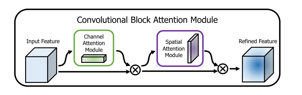
Fig. 1: The overview of CBAM. The module has two sequential sub-modules: channel and spatial. The intermediate feature map is adaptively refined through our module (CBAM) at every convolutional block of deep networks.
图 1:CBAM 概览。该模块有两个依次使用的子模块:通道与空间。在深度网络的每一个卷积块上,中间特征图都经由我们的模块(CBAM)做自适应精炼。
2 Related Work
2 相关工作
Network engineering.
网络结构设计。
“Network engineering” has been one of the most important vision research, because well-designed networks ensure remarkable performance improvement in various applications. A wide range of architectures has been proposed since the successful implementation of a large-scale CNN [19]. An intuitive and simple way of extension is to increase the depth of neural networks [9]. Szegedy et al. [10] introduce a deep Inception network using a multi-branch architecture where each branch is customized carefully. While a naive increase in depth comes to saturation due to the difficulty of gradient propagation, ResNet [5] proposes a simple identity skip-connection to ease the optimization issues of deep networks. Based on the ResNet architecture, various models such as WideResNet [6], Inception-ResNet [8], and ResNeXt [7] have been developed. WideResNet [6] proposes a residual network with a larger number of convolutional filters and reduced depth. PyramidNet [20] is a strict generalization of WideResNet where the width of the network gradually increases. ResNeXt [7] suggests to use grouped convolutions and shows that increasing the cardinality leads to better classification accuracy. More recently, Huang et al. [21] propose a new architecture, DenseNet. It iteratively concatenates the input features with the output features, enabling each convolution block to receive raw information from all the previous blocks. While most of recent network engineering methods mainly target on three factors depth [19,9,10,5], width [10,22,6,8], and cardinality [7,11], we focus on the other aspect, ‘attention’, one of the curious facets of a human visual system.
“网络结构设计”一直是视觉研究中最重要的方向之一,因为设计得当的网络能在多种应用上带来显著的性能提升。自从大规模 CNN 成功实现以来 [19],已经出现了多种多样的结构。一种直观而简单的扩展方式是增加神经网络的深度 [9]。Szegedy 等人 [10] 提出深度 Inception 网络,采用多分支结构,并为每个分支仔细定制。单纯加深会因梯度传播困难而趋于饱和,ResNet [5] 于是提出简单的恒等跳跃连接,以缓解深层网络的优化问题。在 ResNet 结构之上,又发展出 WideResNet [6]、Inception-ResNet [8] 和 ResNeXt [7] 等多种模型。WideResNet [6] 提出卷积滤波器更多、深度更浅的残差网络。PyramidNet [20] 是 WideResNet 的严格推广,网络宽度逐步增加。ResNeXt [7] 建议使用分组卷积,并表明增加基数能提高分类精度。更近一些,Huang 等人 [21] 提出新的结构 DenseNet。它反复把输入特征与输出特征拼接起来,使每个卷积块都能接收到来自此前所有块的原始信息。近期多数网络结构设计主要针对深度 [19,9,10,5]、宽度 [10,22,6,8] 和基数 [7,11] 这三个因素,而我们把目光放在另一个方面——“注意力”,这是人类视觉系统中一个引人好奇的侧面。
Attention mechanism.
注意力机制。
It is well known that attention plays an important role in human perception [23,24,25]. One important property of a human visual system is that one does not attempt to process a whole scene at once. Instead, humans exploit a sequence of partial glimpses and selectively focus on salient parts in order to capture visual structure better [26].
众所周知,注意力在人类感知中起着重要作用 [23,24,25]。人类视觉系统的一个重要特性是,人并不会试图一次处理整个场景。相反,人会利用一连串局部瞥视,有选择地把注意力放在显著部位上,以便更好地把握视觉结构 [26]。
Recently, there have been several attempts [27,28] to incorporate attention processing to improve the performance of CNNs in large-scale classification tasks. Wang et al. [27] propose Residual Attention Network which uses an encoder-decoder style attention module. By refining the feature maps, the network not only performs well but is also robust to noisy inputs. Instead of directly computing the 3d attention map, we decompose the process that learns channel attention and spatial attention separately. The separate attention generation process for 3D feature map has much less computational and parameter overhead, and therefore can be used as a plug-and-play module for pre-existing base CNN architectures.
近来已有若干工作 [27,28] 把注意力处理引入 CNN,以提升大规模分类任务上的性能。Wang 等人 [27] 提出 Residual Attention Network,使用编码器–解码器风格的注意力模块。通过对特征图做精炼,该网络不仅效果好,对含噪输入也更稳健。我们并不直接计算三维注意力图,而是把学习过程拆开,分别学习通道注意力和空间注意力。对三维特征图分开生成注意力,计算和参数开销要小得多,因此可以作为即插即用的模块,加到已有的基础 CNN 结构上。
More close to our work, Hu et al. [28] introduce a compact module to exploit the inter-channel relationship. In their Squeeze-and-Excitation module, they use global average-pooled features to compute channel-wise attention. However, we show that those are suboptimal features in order to infer fine channel attention, and we suggest to use max-pooled features as well. They also miss the spatial attention, which plays an important role in deciding ‘where’ to focus as shown in [29]. In our CBAM, we exploit both spatial and channel-wise attention based on an efficient architecture and empirically verify that exploiting both is superior to using only the channel-wise attention as [28]. Moreover, we empirically show that our module is effective in detection tasks (MS-COCO and VOC). Especially, we achieve state-of-the-art performance just by placing our module on top of the existing one-shot detector [30] in the VOC2007 test set.
与我们更接近的是 Hu 等人 [28] 提出的紧凑模块,用来利用通道之间的关系。在他们的 Squeeze-and-Excitation 模块里,用全局平均池化后的特征来计算通道注意力。但我们表明,仅用这些特征来推断精细的通道注意力并不是最优的,并建议同时使用最大池化特征。他们也没有考虑空间注意力,而如 [29] 所示,空间注意力在决定“看哪里”时起着重要作用。在 CBAM 中,我们基于高效的结构同时利用空间注意力和通道注意力,并用实验验证:两者一起用,优于像 [28] 那样只使用通道注意力。此外,我们还通过实验表明,该模块在检测任务(MS COCO 和 VOC)上同样有效。尤其是在 VOC 2007 测试集上,只需把模块加到已有的单次检测器 [30] 上,就能达到当时最好的性能。
Concurrently, BAM [31] takes a similar approach, decomposing 3D attention map inference into channel and spatial. They place BAM module at every bottleneck of the network while we plug at every convolutional block.
与此同时,BAM [31] 采取了类似的思路,把三维注意力图的推断拆成通道和空间。他们把 BAM 模块放在网络的每一个瓶颈处,而我们则插入每一个卷积块。
3 Convolutional Block Attention Module
3 卷积块注意力模块
Given an intermediate feature map as input, CBAM sequentially infers a 1D channel attention map and a 2D spatial attention map as illustrated in Fig. 1. The overall attention process can be summarized as:
where denotes element-wise multiplication. During multiplication, the attention values are broadcasted (copied) accordingly: channel attention values are broadcasted along the spatial dimension, and vice versa. is the final refined output. Fig. 2 depicts the computation process of each attention map. The following describes the details of each attention module.
给定中间特征图 作为输入,CBAM 依次推断一维通道注意力图 和二维空间注意力图 ,如图 1 所示。整个注意力过程可以概括为:
其中 表示逐元素相乘。相乘时,注意力值会相应地广播(复制):通道注意力沿空间维度广播,空间注意力则沿通道维度广播。 是最终精炼后的输出。图 2 画出了每张注意力图的计算过程。下面分别说明两个注意力模块的细节。
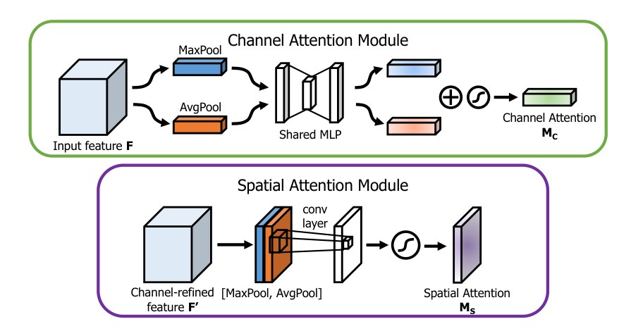
Fig. 2: Diagram of each attention sub-module. As illustrated, the channel sub-module utilizes both max-pooling outputs and average-pooling outputs with a shared network; the spatial sub-module utilizes similar two outputs that are pooled along the channel axis and forward them to a convolution layer.
图 2:各个注意力子模块的示意。如图所示,通道子模块同时使用最大池化和平均池化的输出,并交给一个共享网络;空间子模块则使用沿通道轴池化得到的类似两路输出,再把它们送入一层卷积。
Channel attention module.
通道注意力模块。
We produce a channel attention map by exploiting the inter-channel relationship of features. As each channel of a feature map is considered as a feature detector [32], channel attention focuses on ‘what’ is meaningful given an input image. To compute the channel attention efficiently, we squeeze the spatial dimension of the input feature map. For aggregating spatial information, average-pooling has been commonly adopted so far. Zhou et al. [33] suggest to use it to learn the extent of the target object effectively and Hu et al. [28] adopt it in their attention module to compute spatial statistics. Beyond the previous works, we argue that max-pooling gathers another important clue about distinctive object features to infer finer channel-wise attention. Thus, we use both average-pooled and max-pooled features simultaneously. We empirically confirmed that exploiting both features greatly improves representation power of networks rather than using each independently (see Sec. 4.1), showing the effectiveness of our design choice. We describe the detailed operation below.
我们利用特征在通道之间的关系来生成通道注意力图。特征图的每个通道都可以看成一个特征检测器 [32],因此通道注意力关注的是:给定输入图像时,“什么”是有意义的。为了高效计算通道注意力,我们压缩输入特征图的空间维度。在汇聚空间信息时,以往普遍采用平均池化。Zhou 等人 [33] 建议用它来有效学习目标物体的范围,Hu 等人 [28] 也在其注意力模块里用它来计算空间统计量。在已有工作之外,我们认为最大池化还能收集关于显著物体特征的另一类重要线索,从而推断出更精细的通道注意力。因此我们同时使用平均池化和最大池化后的特征。实验证实,同时利用这两种特征,比各自单独使用更能提升网络的表征能力(见第 4.1 节),说明了这一设计选择的有效性。具体运算如下。
We first aggregate spatial information of a feature map by using both average-pooling and max-pooling operations, generating two different spatial context descriptors: and , which denote average-pooled features and max-pooled features respectively. Both descriptors are then forwarded to a shared network to produce our channel attention map . The shared network is composed of multi-layer perceptron (MLP) with one hidden layer. To reduce parameter overhead, the hidden activation size is set to , where is the reduction ratio. After the shared network is applied to each descriptor, we merge the output feature vectors using element-wise summation. In short, the channel attention is computed as:
where denotes the sigmoid function, , and . Note that the MLP weights, and , are shared for both inputs and the ReLU activation function is followed by .
我们先用平均池化和最大池化两种运算汇聚特征图的空间信息,得到两个不同的空间上下文描述子: 和 ,分别表示平均池化特征和最大池化特征。两个描述子随后被送入一个共享网络,以产生通道注意力图 。共享网络是带一个隐层的多层感知机(MLP)。为减少参数开销,隐层激活的尺寸设为 ,其中 是缩减比。共享网络分别作用于每个描述子后,再用逐元素相加合并输出特征向量。简言之,通道注意力的计算为:
其中 表示 sigmoid 函数,,。注意,MLP 的权重 和 对两路输入是共享的,并且 之后接 ReLU 激活函数。
Spatial attention module.
空间注意力模块。
We generate a spatial attention map by utilizing the inter-spatial relationship of features. Different from the channel attention, the spatial attention focuses on ‘where’ is an informative part, which is complementary to the channel attention. To compute the spatial attention, we first apply average-pooling and max-pooling operations along the channel axis and concatenate them to generate an efficient feature descriptor. Applying pooling operations along the channel axis is shown to be effective in highlighting informative regions [34]. On the concatenated feature descriptor, we apply a convolution layer to generate a spatial attention map which encodes where to emphasize or suppress. We describe the detailed operation below.
我们利用特征在空间上的相互关系来生成空间注意力图。与通道注意力不同,空间注意力关注的是“哪里”是有信息的部位,与通道注意力形成互补。为了计算空间注意力,我们先沿通道轴做平均池化和最大池化,再把结果拼接起来,得到一个高效的特征描述子。沿通道轴做池化,已被表明能有效突出有信息的区域 [34]。在拼接后的特征描述子上,我们再接一层卷积,生成空间注意力图 ,用来编码该强调或抑制哪些位置。具体运算如下。
We aggregate channel information of a feature map by using two pooling operations, generating two 2D maps: and . Each denotes average-pooled features and max-pooled features across the channel. Those are then concatenated and convolved by a standard convolution layer, producing our 2D spatial attention map. In short, the spatial attention is computed as:
where denotes the sigmoid function and represents a convolution operation with the filter size of .
我们用两种池化运算汇聚特征图的通道信息,得到两张二维图: 和 ,分别表示沿通道的平均池化特征和最大池化特征。二者拼接后,再经一层标准卷积,得到二维空间注意力图。简言之,空间注意力的计算为:
其中 表示 sigmoid 函数, 表示滤波器大小为 的卷积运算。
Arrangement of attention modules. Given an input image, two attention modules, channel and spatial, compute complementary attention, focusing on ‘what’ and ‘where’ respectively. Considering this, two modules can be placed in a parallel or sequential manner. We found that the sequential arrangement gives a better result than a parallel arrangement. For the arrangement of the sequential process, our experimental result shows that the channel-first order is slightly better than the spatial-first. We will discuss experimental results on network engineering in Sec. 4.1.
注意力模块的组合方式。 给定一张输入图像,通道和空间这两个注意力模块计算的是互补的注意力,分别关注“什么”和“哪里”。据此,两个模块可以并行放置,也可以顺序放置。我们发现顺序组合优于并行组合。在顺序组合中,实验结果还表明,通道在前略优于空间在前。我们将在第 4.1 节讨论有关网络结构设计的实验结果。
4 Experiments
4 实验
We evaluate CBAM on the standard benchmarks: ImageNet-1K for image classification; MS COCO and VOC 2007 for object detection. In order to perform better apple-to-apple comparisons, we reproduced all the evaluated networks [5,6,7,35,28] in the PyTorch framework [36] and report our reproduced results in the whole experiments.
我们在标准基准上评估 CBAM:用 ImageNet-1K 做图像分类,用 MS COCO 和 VOC 2007 做目标检测。为了更公平地做对等比较,我们在 PyTorch 框架 [36] 中复现了全部被评估的网络 [5,6,7,35,28],并在全部实验中报告复现结果。
To thoroughly evaluate the effectiveness of our final module, we first perform extensive ablation experiments. Then, we verify that CBAM outperforms all the baselines without bells and whistles, demonstrating the general applicability of CBAM across different architectures as well as different tasks. One can seamlessly integrate CBAM in any CNN architectures and jointly train the combined CBAM-enhanced networks. Fig. 3 shows a diagram of CBAM integrated with a ResBlock in ResNet [5] as an example.
为了彻底评估最终模块的有效性,我们先做大量消融实验。随后我们验证,CBAM 在不加额外技巧的情况下优于所有基线,说明它在不同结构和不同任务上都具有普遍适用性。CBAM 可以无缝插入任意 CNN 结构,并与组合后的网络一起训练。图 3 以 ResNet [5] 中的残差块为例,给出了插入 CBAM 的示意。
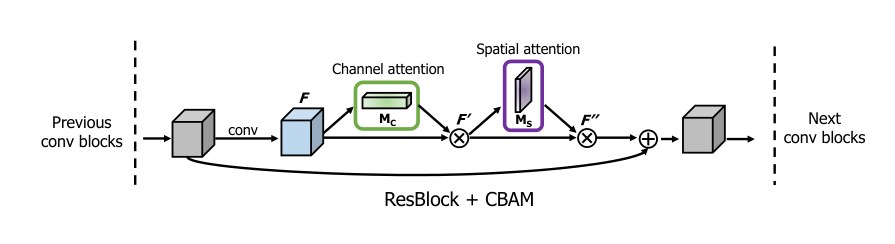
Fig. 3: CBAM integrated with a ResBlock in ResNet[5]. This figure shows the exact position of our module when integrated within a ResBlock. We apply CBAM on the convolution outputs in each block.
图 3:CBAM 插入 ResNet[5] 残差块的方式。本图给出模块集成到残差块中时的准确位置。我们在每个块的卷积输出上施加 CBAM。
4.1 Ablation studies
4.1 消融实验
In this subsection, we empirically show the effectiveness of our design choice. For this ablation study, we use the ImageNet-1K dataset and adopt ResNet-50 [5] as the base architecture. The ImageNet-1K classification dataset [1] consists of 1.2 million images for training and 50,000 for validation with 1,000 object classes. We adopt the same data augmentation scheme with [5,37] for training and apply a single-crop evaluation with the size of 224×224 at test time. The learning rate starts from 0.1 and drops every 30 epochs. We train the networks for 90 epochs. Following [5,37,38], we report classification errors on the validation set.
本小节通过实验说明我们设计选择的有效性。消融以 ImageNet-1K 为数据、以 ResNet-50 [5] 为基座结构。ImageNet-1K 分类数据集 [1] 有 120 万张训练图像和 5 万张验证图像,共 1,000 个物体类别。训练时采用与 [5,37] 相同的数据增广,测试时做 224×224 的单裁剪评估。学习率从 0.1 起,每 30 个 epoch 下降一次,共训练 90 个 epoch。按照 [5,37,38],我们在验证集上报告分类错误率。
Our module design process is split into three parts. We first search for the effective approach to computing the channel attention, then the spatial attention. Finally, we consider how to combine both channel and spatial attention modules. We explain the details of each experiment below.
模块设计过程分成三部分。我们先寻找有效的通道注意力计算方法,再看空间注意力,最后考虑如何组合这两个注意力模块。下面分别说明各实验的细节。
Channel attention.
通道注意力。
We experimentally verify that using both average-pooled and max-pooled features enables finer attention inference. We compare 3 variants of channel attention: average pooling, max pooling, and joint use of both poolings. Note that the channel attention module with an average pooling is the same as the SE [28] module. Also, when using both poolings, we use a shared MLP for attention inference to save parameters, as both of aggregated channel features lie in the same semantic embedding space. We only use channel attention modules in this experiment and we fix the reduction ratio to 16.
我们通过实验验证:同时使用平均池化和最大池化特征,能够做出更精细的注意力推断。我们比较通道注意力的三种变体:平均池化、最大池化,以及两者联用。需要注意,只使用平均池化的通道注意力模块与 SE [28] 模块相同。另外,在同时使用两种池化时,我们用共享的 MLP 来推断注意力以节省参数,因为两路汇聚后的通道特征位于同一语义嵌入空间。本实验只使用通道注意力模块,并把缩减比固定为 16。
| Description | Parameters | GFLOPs | Top-1 Error(%) | Top-5 Error(%) |
|---|---|---|---|---|
| ResNet50 (baseline) | 25.56M | 3.86 | 24.56 | 7.50 |
| ResNet50 + AvgPool (SE [28]) | 25.92M | 3.94 | 23.14 | 6.70 |
| ResNet50 + MaxPool | 25.92M | 3.94 | 23.20 | 6.83 |
| ResNet50 + AvgPool & MaxPool | 25.92M | 4.02 | 22.80 | 6.52 |
Table 1: Comparison of different channel attention methods. We observe that using our proposed method outperforms recently suggested Squeeze and Excitation method [28].
| Description | Parameters | GFLOPs | Top-1 Error(%) | Top-5 Error(%) |
|---|---|---|---|---|
| ResNet50 (baseline) | 25.56M | 3.86 | 24.56 | 7.50 |
| ResNet50 + AvgPool (SE [28]) | 25.92M | 3.94 | 23.14 | 6.70 |
| ResNet50 + MaxPool | 25.92M | 3.94 | 23.20 | 6.83 |
| ResNet50 + AvgPool & MaxPool | 25.92M | 4.02 | 22.80 | 6.52 |
表 1: 不同通道注意力方法的比较。我们观察到,所提方法优于近期提出的 Squeeze-and-Excitation 方法 [28]。
Experimental results with various pooling methods are shown in Table 1. We observe that max-pooled features are as meaningful as average-pooled features, comparing the accuracy improvement from the baseline. In the work of SE [28], however, they only exploit the average-pooled features, missing the importance of max-pooled features. We argue that max-pooled features which encode the degree of the most salient part can compensate the average-pooled features which encode global statistics softly. Thus, we suggest to use both features simultaneously and apply a shared network to those features. The outputs of a shared network are then merged by element-wise summation. We empirically show that our channel attention method is an effective way to push performance further from SE [28] without additional learnable parameters. As a brief conclusion, we use both average- and max-pooled features in our channel attention module with the reduction ratio of 16 in the following experiments.
表 1 给出了不同池化方法的实验结果。从相对基线的精度提升来看,最大池化特征与平均池化特征同样有意义。然而在 SE [28] 中,他们只利用了平均池化特征,忽略了最大池化特征的重要性。我们认为,最大池化特征编码的是最显著部位的强度,可以补充平均池化特征对全局统计的较软刻画。因此我们建议同时使用这两种特征,并用一个共享网络作用于它们,再把共享网络的输出逐元素相加合并。实验表明,我们的通道注意力方法能在 SE [28] 之上进一步提升性能,而且不增加可学习参数。简要的结论是:在后续实验中,通道注意力模块同时使用平均池化和最大池化特征,缩减比为 16。
Spatial attention.
空间注意力。
Given the channel-wise refined features, we explore an effective method to compute the spatial attention. The design philosophy is symmetric with the channel attention branch. To generate a 2D spatial attention map, we first compute a 2D descriptor that encodes channel information at each pixel over all spatial locations. We then apply one convolution layer to the 2D descriptor, obtaining the raw attention map. The final attention map is normalized by the sigmoid function.
在得到按通道精炼后的特征之后,我们探索一种有效的空间注意力计算方法。设计思路与通道注意力分支是对称的。为生成二维空间注意力图,我们先计算一个二维描述子,在每个空间位置上编码该像素处的通道信息,再对这个二维描述子做一层卷积,得到原始注意力图。最终的注意力图用 sigmoid 函数归一化。
We compare two methods of generating the 2D descriptor: channel pooling using average- and max-pooling across the channel axis and standard 1 × 1 convolution reducing the channel dimension into 1. In addition, we investigate the effect of a kernel size at the following convolution layer: kernel sizes of 3 and 7. In the experiment, we place the spatial attention module after the previously designed channel attention module, as the final goal is to use both modules together.
我们比较两种生成二维描述子的方法:沿通道轴做平均池化与最大池化的通道池化,以及把通道维压到 1 的标准 1×1 卷积。此外,我们考察后续卷积层核大小的影响,分别试了 3 和 7。实验中,空间注意力模块放在前面已经设计好的通道注意力模块之后,因为最终目标是两个模块一起使用。
| Description | Param. | GFLOPs | Top-1 Error(%) | Top-5 Error(%) |
|---|---|---|---|---|
| ResNet50 + channel (SE [28]) | 28.09M | 3.860 | 23.14 | 6.70 |
| ResNet50 + channel | 28.09M | 3.860 | 22.80 | 6.52 |
| ResNet50 + channel + spatial (1x1 conv, k=3) | 28.10M | 3.862 | 22.96 | 6.64 |
| ResNet50 + channel + spatial (1x1 conv, k=7) | 28.10M | 3.869 | 22.90 | 6.47 |
| ResNet50 + channel + spatial (avg&max, k=3) | 28.09M | 3.863 | 22.68 | 6.41 |
| ResNet50 + channel + spatial (avg&max, k=7) | 28.09M | 3.864 | 22.66 | 6.31 |
Table 2: Comparison of different spatial attention methods. Using the proposed channel-pooling (i.e. average- and max-pooling along the channel axis) along with the large kernel size of 7 for the following convolution operation performs best.
| Description | Param. | GFLOPs | Top-1 Error(%) | Top-5 Error(%) |
|---|---|---|---|---|
| ResNet50 + channel (SE [28]) | 28.09M | 3.860 | 23.14 | 6.70 |
| ResNet50 + channel | 28.09M | 3.860 | 22.80 | 6.52 |
| ResNet50 + channel + spatial (1x1 conv, k=3) | 28.10M | 3.862 | 22.96 | 6.64 |
| ResNet50 + channel + spatial (1x1 conv, k=7) | 28.10M | 3.869 | 22.90 | 6.47 |
| ResNet50 + channel + spatial (avg&max, k=3) | 28.09M | 3.863 | 22.68 | 6.41 |
| ResNet50 + channel + spatial (avg&max, k=7) | 28.09M | 3.864 | 22.66 | 6.31 |
表 2: 不同空间注意力方法的比较。采用所提出的通道池化(即沿通道轴做平均池化和最大池化),并在后续卷积中使用较大的 7 号核,效果最好。
Table 2 shows the experimental results. We can observe that the channel pooling produces better accuracy, indicating that explicitly modeled pooling leads to finer attention inference rather than learnable weighted channel pooling (implemented as 1 × 1 convolution). In the comparison of different convolution kernel sizes, we find that adopting a larger kernel size generates better accuracy in both cases. It implies that a broad view (i.e. large receptive field) is needed for deciding spatially important regions. Considering this, we adopt the channel-pooling method and the convolution layer with a large kernel size to compute spatial attention. In a brief conclusion, we use the average- and max-pooled features across the channel axis with a convolution kernel size of 7 as our spatial attention module.
表 2 给出了实验结果。可以看到通道池化的精度更好,说明显式建模的池化,比可学习的加权通道池化(实现为 1×1 卷积)更能做出精细的注意力推断。在不同卷积核大小的比较中,两种情形下采用更大的核都得到了更好的精度。这意味着,要判定空间上重要的区域,需要更宽的视野(即更大的感受野)。据此,我们采用通道池化方法,并用大核卷积来计算空间注意力。简要的结论是:空间注意力模块使用沿通道轴的平均池化与最大池化特征,卷积核大小为 7。
Arrangement of the channel and spatial attention.
通道注意力与空间注意力的组合。
In this experiment, we compare three different ways of arranging the channel and spatial attention submodules: sequential channel-spatial, sequential spatial-channel, and parallel use of both attention modules. As each module has different functions, the order may affect the overall performance. For example, from a spatial viewpoint, the channel attention is globally applied, while the spatial attention works locally. Also, it is natural to think that we may combine two attention outputs to build a 3D attention map. In the case, both attentions can be applied in parallel, then the outputs of the two attention modules are added and normalized with the sigmoid function.
本实验比较三种组合通道与空间注意力子模块的方式:通道–空间的顺序组合、空间–通道的顺序组合,以及两个注意力模块并行使用。由于两个模块功能不同,顺序可能影响总体性能。例如,从空间角度看,通道注意力是全局施加的,而空间注意力在局部起作用。另外,自然也会想到把两路注意力输出结合起来,构成三维注意力图。这时可以把两种注意力并行使用,再把两个模块的输出相加,并用 sigmoid 函数归一化。
| Description | Top-1 Error(%) | Top-5 Error(%) |
|---|---|---|
| ResNet50 + channel (SE [28]) | 23.14 | 6.70 |
| ResNet50 + channel + spatial | 22.66 | 6.31 |
| ResNet50 + spatial + channel | 22.78 | 6.42 |
| ResNet50 + channel & spatial in parallel | 22.95 | 6.59 |
Table 3: Combining methods of channel and spatial attention. Using both attention is critical while the best-combining strategy (i.e. sequential, channel-first) further improves the accuracy.
| Description | Top-1 Error(%) | Top-5 Error(%) |
|---|---|---|
| ResNet50 + channel (SE [28]) | 23.14 | 6.70 |
| ResNet50 + channel + spatial | 22.66 | 6.31 |
| ResNet50 + spatial + channel | 22.78 | 6.42 |
| ResNet50 + channel & spatial in parallel | 22.95 | 6.59 |
表 3: 通道注意力与空间注意力的组合方法。同时使用两种注意力至关重要,而最佳组合策略(即顺序、通道在前)还能进一步提高精度。
Table 3 summarizes the experimental results on different attention arranging methods. From the results, we can find that generating an attention map sequentially infers a finer attention map than doing in parallel. In addition, the channel-first order performs slightly better than the spatial-first order. Note that all the arranging methods outperform using only the channel attention independently, showing that utilizing both attentions is crucial while the best-arranging strategy further pushes performance.
表 3 汇总了不同注意力组合方法的实验结果。从结果可以看出,按顺序生成注意力图,比并行方式能推断出更精细的注意力图。此外,通道在前的顺序略优于空间在前。需要注意,所有组合方式都优于单独使用通道注意力,说明同时利用两种注意力至关重要,而最佳组合策略还能把性能再推进一步。
4.2 Image Classification on ImageNet-1K
4.2 ImageNet-1K 上的图像分类
We perform ImageNet-1K classification experiments to rigorously evaluate our module. We follow the same protocol as specified in Sec. 4.1 and evaluate our module in various network architectures including ResNet [5], WideResNet [6], and ResNext [7].
我们在 ImageNet-1K 分类实验上对模块做更严格的评估。协议与第 4.1 节相同,并在多种网络结构上评估,包括 ResNet [5]、WideResNet [6] 和 ResNeXt [7]。
Table 4 summarizes the experimental results. The networks with CBAM outperform all the baselines significantly, demonstrating that the CBAM can generalize well on various models in the large-scale dataset. Moreover, the models with CBAM improve the accuracy upon the one of the strongest method – SE [28] which is the winning approach of the ILSVRC 2017 classification task. It implies that our proposed approach is powerful, showing the efficacy of new pooling method that generates richer descriptor and spatial attention that complements the channel attention effectively.
表 4 汇总了实验结果。加入 CBAM 的网络显著优于所有基线,说明 CBAM 能在大规模数据上很好地推广到多种模型。此外,带 CBAM 的模型还在当时最强方法之一——ILSVRC 2017 分类任务获胜方法 SE [28]——的基础上进一步提高了精度。这说明所提方法是有效的:新的池化方式能生成更丰富的描述子,空间注意力也能有效补充通道注意力。
| Architecture | Param. | GFLOPs | Top-1 Error (%) | Top-5 Error (%) |
|---|---|---|---|---|
| ResNet18 [5] | 11.69M | 1.814 | 29.60 | 10.55 |
| ResNet18 [5] + SE [28] | 11.78M | 1.814 | 29.41 | 10.22 |
| ResNet18 [5] + CBAM | 11.78M | 1.815 | 29.27 | 10.09 |
| ResNet34 [5] | 21.80M | 3.664 | 26.69 | 8.60 |
| ResNet34 [5] + SE [28] | 21.96M | 3.664 | 26.13 | 8.35 |
| ResNet34 [5] + CBAM | 21.96M | 3.665 | 25.99 | 8.24 |
| ResNet50 [5] | 25.56M | 3.858 | 24.56 | 7.50 |
| ResNet50 [5] + SE [28] | 28.09M | 3.860 | 23.14 | 6.70 |
| ResNet50 [5] + CBAM | 28.09M | 3.864 | 22.66 | 6.31 |
| ResNet101 [5] | 44.55M | 7.570 | 23.38 | 6.88 |
| ResNet101 [5] + SE [28] | 49.33M | 7.575 | 22.35 | 6.19 |
| ResNet101 [5] + CBAM | 49.33M | 7.581 | 21.51 | 5.69 |
| WideResNet18 [6] (widen=1.5) | 25.88M | 3.866 | 26.85 | 8.88 |
| WideResNet18 [6] (widen=1.5) + SE [28] | 26.07M | 3.867 | 26.21 | 8.47 |
| WideResNet18 [6] (widen=1.5) + CBAM | 26.08M | 3.868 | 26.10 | 8.43 |
| WideResNet18 [6] (widen=2.0) | 45.62M | 6.696 | 25.63 | 8.20 |
| WideResNet18 [6] (widen=2.0) + SE [28] | 45.97M | 6.696 | 24.93 | 7.65 |
| WideResNet18 [6] (widen=2.0) + CBAM | 45.97M | 6.697 | 24.84 | 7.63 |
| ResNeXt50 [7] (32x4d) | 25.03M | 3.768 | 22.85 | 6.48 |
| ResNeXt50 [7] (32x4d) + SE [28] | 27.56M | 3.771 | 21.91 | 6.04 |
| ResNeXt50 [7] (32x4d) + CBAM | 27.56M | 3.774 | 21.92 | 5.91 |
| ResNeXt101 [7] (32x4d) | 44.18M | 7.508 | 21.54 | 5.75 |
| ResNeXt101 [7] (32x4d) + SE [28] | 48.96M | 7.512 | 21.17 | 5.66 |
| ResNeXt101 [7] (32x4d) + CBAM | 48.96M | 7.519 | 21.07 | 5.59 |
- all results are reproduced in the PyTorch framework.
Table 4: Classification results on ImageNet-1K. Single-crop validation errors are reported.
| Architecture | Param. | GFLOPs | Top-1 Error (%) | Top-5 Error (%) |
|---|---|---|---|---|
| ResNet18 [5] | 11.69M | 1.814 | 29.60 | 10.55 |
| ResNet18 [5] + SE [28] | 11.78M | 1.814 | 29.41 | 10.22 |
| ResNet18 [5] + CBAM | 11.78M | 1.815 | 29.27 | 10.09 |
| ResNet34 [5] | 21.80M | 3.664 | 26.69 | 8.60 |
| ResNet34 [5] + SE [28] | 21.96M | 3.664 | 26.13 | 8.35 |
| ResNet34 [5] + CBAM | 21.96M | 3.665 | 25.99 | 8.24 |
| ResNet50 [5] | 25.56M | 3.858 | 24.56 | 7.50 |
| ResNet50 [5] + SE [28] | 28.09M | 3.860 | 23.14 | 6.70 |
| ResNet50 [5] + CBAM | 28.09M | 3.864 | 22.66 | 6.31 |
| ResNet101 [5] | 44.55M | 7.570 | 23.38 | 6.88 |
| ResNet101 [5] + SE [28] | 49.33M | 7.575 | 22.35 | 6.19 |
| ResNet101 [5] + CBAM | 49.33M | 7.581 | 21.51 | 5.69 |
| WideResNet18 [6] (widen=1.5) | 25.88M | 3.866 | 26.85 | 8.88 |
| WideResNet18 [6] (widen=1.5) + SE [28] | 26.07M | 3.867 | 26.21 | 8.47 |
| WideResNet18 [6] (widen=1.5) + CBAM | 26.08M | 3.868 | 26.10 | 8.43 |
| WideResNet18 [6] (widen=2.0) | 45.62M | 6.696 | 25.63 | 8.20 |
| WideResNet18 [6] (widen=2.0) + SE [28] | 45.97M | 6.696 | 24.93 | 7.65 |
| WideResNet18 [6] (widen=2.0) + CBAM | 45.97M | 6.697 | 24.84 | 7.63 |
| ResNeXt50 [7] (32x4d) | 25.03M | 3.768 | 22.85 | 6.48 |
| ResNeXt50 [7] (32x4d) + SE [28] | 27.56M | 3.771 | 21.91 | 6.04 |
| ResNeXt50 [7] (32x4d) + CBAM | 27.56M | 3.774 | 21.92 | 5.91 |
| ResNeXt101 [7] (32x4d) | 44.18M | 7.508 | 21.54 | 5.75 |
| ResNeXt101 [7] (32x4d) + SE [28] | 48.96M | 7.512 | 21.17 | 5.66 |
| ResNeXt101 [7] (32x4d) + CBAM | 48.96M | 7.519 | 21.07 | 5.59 |
- 全部结果均在 PyTorch 框架中复现。
表 4: ImageNet-1K 上的分类结果。报告的是单裁剪验证错误率。
We also find that the overall overhead of CBAM is quite small in terms of both parameters and computation. This motivates us to apply our proposed module CBAM to the light-weight network, MobileNet [35]. Table 5 summarizes the experimental results that we conducted based on the MobileNet architecture. We have placed CBAM to two models, basic and capacity-reduced model(i.e. adjusting width multiplier(α) to 0.7). We observe similar phenomenon as shown in Table 4. CBAM not only boosts the accuracy of baselines significantly but also favorably improves the performance of SE [28]. This shows the great potential of CBAM for applications on low-end devices.
我们还发现,CBAM 在参数和计算两方面的总体开销都相当小。这促使我们把所提模块应用到轻量网络 MobileNet [35] 上。表 5 汇总了基于 MobileNet 结构的实验结果。我们在两个模型上插入了 CBAM:基本模型,以及把宽度乘数(α)调到 0.7 的容量缩小模型。我们观察到与表 4 类似的现象。CBAM 不仅显著提高了基线精度,也在 SE [28] 之上带来了可观的改进。这说明 CBAM 在低端设备应用上有很大潜力。
| Architecture | Parameters | GFLOPs | Top-1 Error (%) | Top-5 Error (%) |
|---|---|---|---|---|
| MobileNet [35] α = 0.7 | 2.30M | 0.283 | 34.86 | 13.69 |
| MobileNet [35] α = 0.7 + SE [28] | 2.71M | 0.283 | 32.50 | 12.49 |
| MobileNet [35] α = 0.7 + CBAM | 2.71M | 0.289 | 31.51 | 11.48 |
| MobileNet [35] | 4.23M | 0.569 | 31.39 | 11.51 |
| MobileNet [35] + SE [28] | 5.07M | 0.570 | 29.97 | 10.63 |
| MobileNet [35] + CBAM | 5.07M | 0.576 | 29.01 | 9.99 |
- all results are reproduced in the PyTorch framework.
Table 5: Classification results on ImageNet-1K using the light-weight network, MobileNet [35]. Single-crop validation errors are reported.
| Architecture | Parameters | GFLOPs | Top-1 Error (%) | Top-5 Error (%) |
|---|---|---|---|---|
| MobileNet [35] α = 0.7 | 2.30M | 0.283 | 34.86 | 13.69 |
| MobileNet [35] α = 0.7 + SE [28] | 2.71M | 0.283 | 32.50 | 12.49 |
| MobileNet [35] α = 0.7 + CBAM | 2.71M | 0.289 | 31.51 | 11.48 |
| MobileNet [35] | 4.23M | 0.569 | 31.39 | 11.51 |
| MobileNet [35] + SE [28] | 5.07M | 0.570 | 29.97 | 10.63 |
| MobileNet [35] + CBAM | 5.07M | 0.576 | 29.01 | 9.99 |
- 全部结果均在 PyTorch 框架中复现。
表 5: 在轻量网络 MobileNet [35] 上的 ImageNet-1K 分类结果。报告的是单裁剪验证错误率。
4.3 Network Visualization with Grad-CAM [18]
4.3 用 Grad-CAM [18] 做网络可视化
For the qualitative analysis, we apply the Grad-CAM [18] to different networks using images from the ImageNet validation set. Grad-CAM is a recently proposed visualization method which uses gradients in order to calculate the importance of the spatial locations in convolutional layers. As the gradients are calculated with respect to a unique class, Grad-CAM result shows attended regions clearly. By observing the regions that network has considered as important for predicting a class, we attempt to look at how this network is making good use of features. We compare the visualization results of CBAM-integrated network (ResNet50 + CBAM) with baseline (ResNet50) and SE-integrated network (ResNet50 + SE). Fig. 4 illustrate the visualization results. The softmax scores for a target class are also shown in the figure.
为了做定性分析,我们把 Grad-CAM [18] 应用到不同网络上,所用图像来自 ImageNet 验证集。Grad-CAM 是当时新提出的可视化方法,利用梯度来计算卷积层中各空间位置的重要性。由于梯度是相对某一个类别计算的,Grad-CAM 的结果能清楚显示出被关注的区域。通过观察网络在预测某一类时认为重要的区域,我们试图看看这个网络是否很好地利用了特征。我们比较加入 CBAM 的网络(ResNet50 + CBAM)与基线(ResNet50)以及加入 SE 的网络(ResNet50 + SE)的可视化结果。图 4 给出了可视化结果,图中还标出了目标类别的 softmax 分数。
In Fig. 4, we can clearly see that the Grad-CAM masks of the CBAM-integrated network cover the target object regions better than other methods. That is, the CBAM-integrated network learns well to exploit information in target object regions and aggregate features from them. Note that target class scores also increase accordingly.
在图 4 中可以清楚看到,加入 CBAM 的网络,其 Grad-CAM 掩膜比其他方法更好地覆盖了目标物体区域。也就是说,加入 CBAM 的网络更能学会利用目标物体区域中的信息,并从中汇聚特征。需要注意,目标类别的分数也相应地提高了。
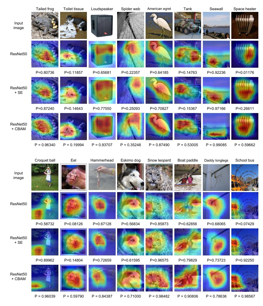
Fig. 4: Grad-CAM [18] visualization results. We compare the visualization results of CBAM-integrated network (ResNet50 + CBAM) with baseline (ResNet50) and SE-integrated network (ResNet50 + SE). The grad-CAM visualization is calculated for the last convolutional outputs. The ground-truth label is shown on the top of each input image and P denotes the softmax score of each network for the ground-truth class.
图 4:Grad-CAM [18] 可视化结果。我们比较加入 CBAM 的网络(ResNet50 + CBAM)与基线(ResNet50)以及加入 SE 的网络(ResNet50 + SE)的可视化结果。Grad-CAM 可视化是对最后一层卷积输出计算的。每张输入图像上方给出真实标签,P 表示各网络对真实类别的 softmax 分数。
4.4 Quantitative evaluation of improved interpretability
4.4 对可解释性改进的定量评估
Following the Sec.5.1 in Grad-CAM paper, we conduct a user study based on Grad-CAM visualizations. We randomly selected 50 images which are correctly classified with both methods(i.e.baseline and CBAM) from ImageNet validation set. The user study is conducted on the Google Forms platform. For each question, randomly shuffled visualizations are shown to the respondents. For the visualizations, regions of the image with Grad-CAM values of 0.6 or greater are shown. In practice, respondents were given full input image, ground-truth label, and two image regions from each methods(see Fig 5). The comparison criterion is “Given class label, which region seems more class-discriminative?”. The respondents can choose that either one is better, or both are similar. There are 50 question sets of images and 25 respondents, resulting in a total of 1250 votes. The results are shown in the Table 6. We can clearly see that CBAM outperforms baseline, showing the improved interpretability.
我们依照 Grad-CAM 论文第 5.1 节,基于 Grad-CAM 可视化做了用户研究。从 ImageNet 验证集中随机抽取 50 张两种方法(即基线与 CBAM)都分类正确的图像。用户研究在 Google Forms 平台上进行。每个问题向被试展示随机打乱顺序的可视化结果。可视化时,只显示 Grad-CAM 值不低于 0.6 的图像区域。实际操作中,被试会看到完整输入图像、真实标签,以及两种方法各自给出的图像区域(见图 5)。比较标准是:“给定类别标签,哪一块看起来更有类别区分度?”被试可以选择其中一种更好,或两者差不多。共有 50 组图像题目和 25 名被试,合计 1250 票。结果见表 6。可以清楚看到 CBAM 优于基线,说明可解释性得到了改进。
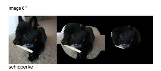
Fig. 5: Example of question image for the user study.
图 5:用户研究中的题目图像示例。
| Survey choice | Votes |
|---|---|
| Seems equal | 295 |
| Baseline better | 288 |
| CBAM better | 667 |
Table 6: Results of user study.
| Survey choice | Votes |
|---|---|
| Seems equal | 295 |
| Baseline better | 288 |
| CBAM better | 667 |
表 6: 用户研究结果。
4.5 MS COCO Object Detection
4.5 MS COCO 目标检测
We conduct object detection on the Microsoft COCO dataset [3]. This dataset involves 80k training images (“2014 train”) and 40k validation images (“2014 val”). The average mAP over different IoU thresholds from 0.5 to 0.95 is used for evaluation. According to [39,40], we trained our model using all the training images as well as a subset of validation images, holding out 5,000 examples for validation. Our training code is based on [41] and we train the network for 490K iterations for fast performance validation. We adopt Faster-RCNN [42] as our detection method and ImageNet pre-trained ResNet50 and ResNet101 [5] as our baseline networks. Here we are interested in performance improvement by plugging CBAM to the baseline networks. Since we use the same detection method in all the models, the gains can only be attributed to the enhanced representation power, given by our module CBAM. As shown in the Table 7, we observe significant improvements from the baseline, demonstrating generalization performance of CBAM on other recognition tasks.
我们在 Microsoft COCO 数据集 [3] 上做目标检测。该数据集包含 8 万张训练图像(“2014 train”)和 4 万张验证图像(“2014 val”)。评价指标是 IoU 阈值从 0.5 到 0.95 的平均 mAP。按照 [39,40],我们用全部训练图像以及一部分验证图像来训练,并留出 5,000 个样本做验证。训练代码基于 [41],为了尽快验证性能,网络训练 490K 次迭代。检测器采用 Faster R-CNN [42],基线网络为在 ImageNet 上预训练的 ResNet50 和 ResNet101 [5]。这里我们关心的是把 CBAM 插入基线网络后的性能提升。由于所有模型使用相同的检测方法,增益只能归因于模块 CBAM 带来的更强表征能力。如表 7 所示,我们观察到相对基线有明显提升,说明 CBAM 在其他识别任务上也具有推广能力。
| Backbone | Detector | mAP@.5 | mAP@.75 | mAP@[.5, .95] |
|---|---|---|---|---|
| ResNet50 [5] | Faster-RCNN [42] | 46.2 | 28.1 | 27.0 |
| ResNet50 [5] + CBAM | Faster-RCNN [42] | 48.2 | 29.2 | 28.1 |
| ResNet101 [5] | Faster-RCNN [42] | 48.4 | 30.7 | 29.1 |
| ResNet101 [5] + CBAM | Faster-RCNN [42] | 50.5 | 32.6 | 30.8 |
- all results are reproduced in the PyTorch framework.
Table 7: Object detection mAP(%) on the MS COCO validation set. We adopt the Faster R-CNN [42] detection framework and apply our module to the base networks. CBAM boosts mAP@[.5, .95] by 0.9 for both baseline networks.
| Backbone | Detector | mAP@.5 | mAP@.75 | mAP@[.5, .95] |
|---|---|---|---|---|
| ResNet50 [5] | Faster-RCNN [42] | 46.2 | 28.1 | 27.0 |
| ResNet50 [5] + CBAM | Faster-RCNN [42] | 48.2 | 29.2 | 28.1 |
| ResNet101 [5] | Faster-RCNN [42] | 48.4 | 30.7 | 29.1 |
| ResNet101 [5] + CBAM | Faster-RCNN [42] | 50.5 | 32.6 | 30.8 |
- 全部结果均在 PyTorch 框架中复现。
表 7: MS COCO 验证集上的目标检测 mAP(%)。我们采用 Faster R-CNN [42] 检测框架,并把模块加到基础网络上。对两个基线网络,CBAM 都把 mAP@[.5, .95] 提高了 0.9。
4.6 VOC 2007 Object Detection
4.6 VOC 2007 目标检测
We further perform experiments on the PASCAL VOC 2007 test set. In this experiment, we apply CBAM to the detectors, while the previous experiments (Table 7) apply our module to the base networks. We adopt the StairNet [30] framework, which is one of the strongest multi-scale method based on the SSD [40]. For the experiment, we reproduce SSD and StairNet in our PyTorch platform in order to estimate performance improvement of CBAM accurately and achieve 77.8% and 78.9% mAP@.5 respectively, which are higher than the original accuracy reported in the original papers. We then place SE [28] and CBAM right before every classifier, refining the final features which are composed of up-sampled global features and corresponding local features before the prediction, enforcing model to adaptively select only the meaningful features. We train all the models on the union set of VOC 2007 trainval and VOC 2012 trainval (“07+12”), and evaluate on the VOC 2007 test set. The total number of training epochs is 250. We use a weight decay of 0.0005 and a momentum of 0.9. In all the experiments, the size of the input image is fixed to 300 for the simplicity.
我们进一步在 PASCAL VOC 2007 测试集上做实验。与前面(表 7)把模块加到基础网络上不同,本实验把 CBAM 加到检测器上。我们采用 StairNet [30] 框架,它是基于 SSD [40] 的最强多尺度方法之一。为了准确估计 CBAM 带来的提升,我们在自己的 PyTorch 平台上复现了 SSD 和 StairNet,分别达到 77.8% 和 78.9% 的 mAP@.5,高于原论文报告的精度。随后我们把 SE [28] 和 CBAM 放在每一个分类器之前,对由上采样全局特征和相应局部特征组成、用于预测的最终特征做精炼,促使模型自适应地只选择有意义的特征。所有模型都在 VOC 2007 trainval 与 VOC 2012 trainval 的并集(“07+12”)上训练,并在 VOC 2007 测试集上评估。训练共 250 个 epoch,权重衰减为 0.0005,动量为 0.9。为简单起见,全部实验中输入图像大小固定为 300。
The experimental results are summarized in Table 8. We can clearly see that CBAM improves the accuracy of all strong baselines with two backbone networks. Note that accuracy improvement of CBAM comes with a negligible parameter overhead, indicating that enhancement is not due to a naive capacity-increment but because of our effective feature refinement. In addition, the result using the light-weight backbone network [35] again shows that CBAM can be an interesting method to low-end devices.
实验结果汇总于表 8。可以清楚看到,在两个骨干网络上,CBAM 都提高了所有强基线的精度。需要注意,CBAM 带来的精度提升只伴随可忽略的参数开销,说明改进并非来自简单地增加容量,而是来自有效的特征精炼。此外,使用轻量骨干网络 [35] 的结果再次表明,CBAM 对低端设备也可能是一种有价值的方法。
| Backbone | Detector | mAP@.5 | Parameters (M) |
|---|---|---|---|
| VGG16 [9] | SSD [40] | 77.8 | 26.5 |
| VGG16 [9] | StairNet [30] | 78.9 | 32.0 |
| VGG16 [9] | StairNet [30] + SE [28] | 79.1 | 32.1 |
| VGG16 [9] | StairNet [30] + CBAM | 79.3 | 32.1 |
| MobileNet [35] | SSD [40] | 68.1 | 5.81 |
| MobileNet [35] | StairNet [30] | 70.1 | 5.98 |
| MobileNet [35] | StairNet [30] + SE [28] | 70.0 | 5.99 |
| MobileNet [35] | StairNet [30] + CBAM | 70.5 | 6.00 |
- all results are reproduced in the PyTorch framework.
Table 8: Object detection mAP(%) on the VOC 2007 test set. We adopt the StairNet [30] detection framework and apply SE and CBAM to the detectors. CBAM favorably improves all the strong baselines with negligible additional parameters.
| Backbone | Detector | mAP@.5 | Parameters (M) |
|---|---|---|---|
| VGG16 [9] | SSD [40] | 77.8 | 26.5 |
| VGG16 [9] | StairNet [30] | 78.9 | 32.0 |
| VGG16 [9] | StairNet [30] + SE [28] | 79.1 | 32.1 |
| VGG16 [9] | StairNet [30] + CBAM | 79.3 | 32.1 |
| MobileNet [35] | SSD [40] | 68.1 | 5.81 |
| MobileNet [35] | StairNet [30] | 70.1 | 5.98 |
| MobileNet [35] | StairNet [30] + SE [28] | 70.0 | 5.99 |
| MobileNet [35] | StairNet [30] + CBAM | 70.5 | 6.00 |
- 全部结果均在 PyTorch 框架中复现。
表 8: VOC 2007 测试集上的目标检测 mAP(%)。我们采用 StairNet [30] 检测框架,并把 SE 和 CBAM 加到检测器上。CBAM 在几乎不增加参数的情况下,对所有强基线都带来了可观的改进。
5 Conclusion
5 结论
We have presented the convolutional block attention module (CBAM), a new approach to improve representation power of CNN networks. We apply attention-based feature refinement with two distinctive modules, channel and spatial, and achieve considerable performance improvement while keeping the overhead small. For the channel attention, we suggest to use the max-pooled features along with the average-pooled features, leading to produce finer attention than SE [28]. We further push the performance by exploiting the spatial attention. Our final module (CBAM) learns what and where to emphasize or suppress and refines intermediate features effectively. To verify its efficacy, we conducted extensive experiments with various state-of-the-art models and confirmed that CBAM outperforms all the baselines on three different benchmark datasets: ImageNet-1K, MS COCO, and VOC 2007. In addition, we visualize how the module exactly infers given an input image. Interestingly, we observed that our module induces the network to focus on target object properly. We hope CBAM become an important component of various network architectures.
我们提出了卷积块注意力模块(CBAM),这是一种增强 CNN 网络表征能力的新方法。我们用通道和空间两个不同的模块做基于注意力的特征精炼,在把开销保持得很小的同时,获得了可观的性能提升。对于通道注意力,我们建议在平均池化特征之外同时使用最大池化特征,从而得到比 SE [28] 更精细的注意力。我们还通过引入空间注意力把性能再推进一步。最终的模块(CBAM)会学习该强调或抑制“什么”以及“哪里”,并有效精炼中间特征。为验证其有效性,我们在多种当时最好的模型上做了大量实验,并确认 CBAM 在三个不同基准数据集上优于所有基线:ImageNet-1K、MS COCO 和 VOC 2007。此外,我们还可视化了给定输入图像时模块究竟如何推断。有意思的是,我们观察到该模块会引导网络把注意力正确地放在目标物体上。希望 CBAM 能成为多种网络结构中的重要组件。
Acknowledgement
致谢
This work was supported by the Technology Innovation Program (No. 10048320), funded by the Ministry of Trade, Industry & Energy (MI, Korea).
本研究得到韩国产业通商资源部(MI, Korea)资助的技术革新计划(编号 10048320)支持。
References
参考文献
[1] Deng, J., Dong, W., Socher, R., Li, L.J., Li, K., Fei-Fei, L.: Imagenet: A large-scale hierarchical image database. In: Proc. of Computer Vision and Pattern Recognition (CVPR). (2009) 1, 7
[2] Krizhevsky, A., Hinton, G.: Learning multiple layers of features from tiny images 1
[3] Lin, T.Y., Maire, M., Belongie, S., Hays, J., Perona, P., Ramanan, D., Dollár, P., Zitnick, C.L.: Microsoft coco: Common objects in context. In: Proc. of European Conf. on Computer Vision (ECCV). (2014) 1, 13
[4] LeCun, Y., Bottou, L., Bengio, Y., Haffner, P.: Gradient-based learning applied to document recognition. Proceedings of the IEEE 86(11) (1998) 2278–2324 1
[5] He, K., Zhang, X., Ren, S., Sun, J.: Deep residual learning for image recognition. In: Proc. of Computer Vision and Pattern Recognition (CVPR). (2016) 1, 3, 6, 7, 9, 10, 13, 14
[6] Zagoruyko, S., Komodakis, N.: Wide residual networks. arXiv preprint arXiv:1605.07146 (2016) 1, 3, 6, 9, 10
[7] Xie, S., Girshick, R., Dollár, P., Tu, Z., He, K.: Aggregated residual transformations for deep neural networks. arXiv preprint arXiv:1611.05431 (2016) 1, 2, 3, 6, 9, 10
[8] Szegedy, C., Ioffe, S., Vanhoucke, V., Alemi, A.A.: Inception-v4, inception-resnet and the impact of residual connections on learning. In: Proc. of Association for the Advancement of Artificial Intelligence (AAAI). (2017) 1, 3
[9] Simonyan, K., Zisserman, A.: Very deep convolutional networks for large-scale image recognition. arXiv preprint arXiv:1409.1556 (2014) 1, 3, 14
[10] Szegedy, C., Liu, W., Jia, Y., Sermanet, P., Reed, S., Anguelov, D., Erhan, D., Vanhoucke, V., Rabinovich, A.: Going deeper with convolutions. In: Proc. of Computer Vision and Pattern Recognition (CVPR). (2015) 1, 3
[11] Chollet, F.: Xception: Deep learning with depthwise separable convolutions. arXiv preprint arXiv:1610.02357 (2016) 2, 3
[12] Mnih, V., Heess, N., Graves, A., et al.: Recurrent models of visual attention." advances in neural information processing systems. In: Proc. of Neural Information Processing Systems (NIPS). (2014) 2
[13] Ba, J., Mnih, V., Kavukcuoglu, K.: Multiple object recognition with visual attention. (2014) 2
[14] Bahdanau, D., Cho, K., Bengio, Y.: Neural machine translation by jointly learning to align and translate. (2014) 2
[15] Xu, K., Ba, J., Kiros, R., Cho, K., Courville, A., Salakhudinov, R., Zemel, R., Bengio, Y.: Show, attend and tell: Neural image caption generation with visual attention. (2015) 2
[16] Gregor, K., Danihelka, I., Graves, A., Rezende, D.J., Wierstra, D.: Draw: A recurrent neural network for image generation. (2015) 2
[17] Jaderberg, M., Simonyan, K., Zisserman, A., et al.: Spatial transformer networks. In: Proc. of Neural Information Processing Systems (NIPS). (2015) 2
[18] Selvaraju, R.R., Cogswell, M., Das, A., Vedantam, R., Parikh, D., Batra, D.: Grad-cam: Visual explanations from deep networks via gradient-based localization. In: Proceedings of the IEEE Conference on Computer Vision and Pattern Recognition. (2017) 618–626 2, 10, 12
[19] Krizhevsky, A., Sutskever, I., Hinton, G.E.: Imagenet classification with deep convolutional neural networks. In: Proc. of Neural Information Processing Systems (NIPS). (2012) 3
[20] Han, D., Kim, J., Kim, J.: Deep pyramidal residual networks. In: Proc. of Computer Vision and Pattern Recognition (CVPR). (2017) 3
[21] Huang, G., Liu, Z., Weinberger, K.Q., van der Maaten, L.: Densely connected convolutional networks. arXiv preprint arXiv:1608.06993 (2016) 3
[22] Szegedy, C., Vanhoucke, V., Ioffe, S., Shlens, J., Wojna, Z.: Rethinking the inception architecture for computer vision. In: Proc. of Computer Vision and Pattern Recognition (CVPR). (2016) 3
[23] Itti, L., Koch, C., Niebur, E.: A model of saliency-based visual attention for rapid scene analysis. In: IEEE Trans. Pattern Anal. Mach. Intell. (TPAMI). (1998) 3
[24] Rensink, R.A.: The dynamic representation of scenes. In: Visual cognition 7.1-3. (2000) 3
[25] Corbetta, M., Shulman, G.L.: Control of goal-directed and stimulus-driven attention in the brain. In: Nature reviews neuroscience 3.3. (2002) 3
[26] Larochelle, H., Hinton, G.E.: Learning to combine foveal glimpses with a third-order boltzmann machine. In: Proc. of Neural Information Processing Systems (NIPS). (2010) 3
[27] Wang, F., Jiang, M., Qian, C., Yang, S., Li, C., Zhang, H., Wang, X., Tang, X.: Residual attention network for image classification. arXiv preprint arXiv:1704.06904 (2017) 3, 4
[28] Hu, J., Shen, L., Sun, G.: Squeeze-and-excitation networks. arXiv preprint arXiv:1709.01507 (2017) 3, 4, 5, 6, 7, 8, 9, 10, 11, 13, 14
[29] Chen, L., Zhang, H., Xiao, J., Nie, L., Shao, J., Chua, T.S.: Sca-cnn: Spatial and channel-wise attention in convolutional networks for image captioning. In: Proc. of Computer Vision and Pattern Recognition (CVPR). (2017) 4
[30] Sanghyun, W., Soonmin, H., So, K.I.: Stairnet: Top-down semantic aggregation for accurate one shot detection. In: Proc. of Winter Conference on Applications of Computer Vision (WACV). (2018) 4, 13, 14
[31] Park, J., Woo, S., Lee, J.Y., Kweon, I.S.: Bam: Bottleneck attention module. In: Proc. of British Machine Vision Conference (BMVC). (2018) 4
[32] Zeiler, M.D., Fergus, R.: Visualizing and understanding convolutional networks. In: Proc. of European Conf. on Computer Vision (ECCV). (2014) 4
[33] Zhou, B., Khosla, A., Lapedriza, A., Oliva, A., Torralba, A.: Learning deep features for discriminative localization. In: Computer Vision and Pattern Recognition (CVPR), 2016 IEEE Conference on, IEEE (2016) 2921–2929 5
[34] Zagoruyko, S., Komodakis, N.: Paying more attention to attention: Improving the performance of convolutional neural networks via attention transfer. In: ICLR. (2017) 6
[35] Howard, A.G., Zhu, M., Chen, B., Kalenichenko, D., Wang, W., Weyand, T., Andreetto, M., Adam, H.: Mobilenets: Efficient convolutional neural networks for mobile vision applications. arXiv preprint arXiv:1704.04861 (2017) 6, 10, 11, 13, 14
[36] : Pytorch. http://pytorch.org/ Accessed: 2017-11-08. 6
[37] He, K., Zhang, X., Ren, S., Sun, J.: Identity mappings in deep residual networks. In: Proc. of European Conf. on Computer Vision (ECCV). (2016) 7
[38] Huang, G., Sun, Y., Liu, Z., Sedra, D., Weinberger, K.Q.: Deep networks with stochastic depth. In: Proc. of European Conf. on Computer Vision (ECCV). (2016) 7
[39] Bell, S., Lawrence Zitnick, C., Bala, K., Girshick, R.: Inside-outside net: Detecting objects in context with skip pooling and recurrent neural networks. In: Proc. of Computer Vision and Pattern Recognition (CVPR). (2016) 13
[40] Liu, W., Anguelov, D., Erhan, D., Szegedy, C., Reed, S., Fu, C.Y., Berg, A.C.: Ssd: Single shot multibox detector. In: Proc. of European Conf. on Computer Vision (ECCV). (2016) 13, 14
[41] Chen, X., Gupta, A.: An implementation of faster rcnn with study for region sampling. arXiv preprint arXiv:1702.02138 (2017) 13
[42] Ren, S., He, K., Girshick, R., Sun, J.: Faster r-cnn: Towards real-time object detection with region proposal networks. In: Proc. of Neural Information Processing Systems (NIPS). (2015) 13, 14