Causal Structure Learning for Dynamical Systems with Theoretical Score Analysis
Causal Structure Learning for Dynamical Systems with Theoretical Score Analysis
面向动力系统的因果结构学习及理论分数分析
Nicholas Tagliapietra Katharina Ensinger Christoph Zimmer Osman Mian
Abstract
摘要
Real world systems evolve in continuous-time according to their underlying causal relationships, yet their dynamics are often unknown. Existing approaches to learning such dynamics typically either discretize time —leading to poor performance on irregularly sampled data— or ignore the underlying causality. We propose CaDyT , a novel method for causal discovery on dynamical systems addressing both these challenges. In contrast to state-of-the-art causal discovery methods that model the problem using discrete-time Dynamic Bayesian networks, our formulation is grounded in Difference-based causal models, which allow milder assumptions for modeling the continuous nature of the system. CaDyT leverages exact Gaussian Process inference for modeling the continuous-time dynamics which is more aligned with the underlying dynamical process. We propose a practical instantiation that identifies the causal structure via a greedy search guided by the Algorithmic Markov Condition and Minimum Description Length principle. Our experiments show that CaDyT outperforms state-of-the-art methods on both regularly and irregularly-sampled data, discovering causal networks closer to the true underlying dynamics.
现实世界中的系统按底层因果关系在连续时间中演化,但其动力学往往未知。现有学习这类动力学的方法,通常要么把时间离散化——因而在不规则采样数据上表现较差——要么忽略底层因果。我们提出 CaDyT,一种面向动力系统的因果发现新方法,同时处理这两个问题。与用离散时间动态贝叶斯网对问题建模的现有因果发现方法不同,我们的表述建立在基于差分的因果模型之上,对系统的连续性质只需更温和的假设。CaDyT 借助精确的高斯过程推断来建模连续时间动力学,从而更贴合底层动力学过程。我们给出一种可实用的实例化:在算法马尔可夫条件与最短描述长度原则的指导下,用贪心搜索识别因果结构。实验表明,CaDyT 在规则与不规则采样数据上都优于现有方法,发现的因果网络更接近真实的底层动力学。
1Bosch Center for Artificial Intelligence, Renningen, Germany
2Computer Science Department, TU Darmstadt, Germany
3Baden-Wuerttemberg Cooperative State University Mannheim, Germany
4Institute for AI in medicine IKIM, Germany
tagliapietra.nicholas@gmail.com
1 Introduction
1 引言
Real-world physical systems are fundamentally governed by continuous-time dynamics (Strogatz 2000) with intrinsic causal mechanisms. For instance, in a mass-spring system as shown in Figure n:1, the position of each mass () induces a force influencing its own velocity () and the velocities of other masses connected to it with a spring. The position of each mass, however, depends only on its own velocity. This example remarks the importance of incorporating the directionality of causal relationships to achieve physical plausiblity in learned models. While differential equations are the de facto standard for modeling dynamical systems, inferring them from data remains challenging. Moreover, when leveraging data-driven approaches such as neural networks or Gaussian processes to learn these models, there are rarely guarantees that the true underlying dynamics will include causality, and spurious correlations might be incorporated by accident. These challenges highlight the need for a causal discovery framework for learning systems in continuous time.
现实世界中的物理系统,本质上由带有内在因果机制的连续时间动力学所支配(Strogatz 2000)。例如,如图 1 所示的质量-弹簧系统中,每个质量的位置()会产生力,从而影响它自身的速度(),以及通过弹簧与它相连的其他质量的速度。而每个质量的位置,却只依赖于它自己的速度。这个例子说明,要把物理上说得通的关系写进学到的模型,就必须纳入因果关系的方向。微分方程是建模动力系统的通行做法,但从数据中把它们推断出来仍然困难。此外,当用神经网络或高斯过程这类数据驱动方法来学习这些模型时,很少能保证真实底层动力学里包含因果,虚假相关也可能被一并写进去。这些困难表明,需要一套面向连续时间系统学习的因果发现框架。
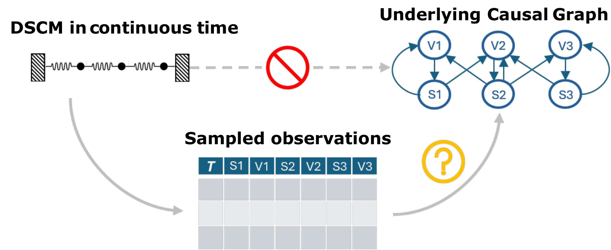
Figure 1: CaDyT discovers the unknown causal structure (Top-right) using trajectories sampled from a continuous-time dynamical system (e.g. n-mass spring system). Our learned continuous-time model adapts to arbitrary timelines, including irregularly sampled ones.
图 1:CaDyT 利用从连续时间动力系统(例如 质量弹簧系统)采样得到的轨迹,发现未知的因果结构(右上)。我们学到的连续时间模型可以适应任意时间轴,也包括不规则采样的时间轴。
Existing state-of-the-art for causal discovery on time-series focuses on learning the causal structure, but rarely captures the underlying continuous dynamics. Indeed, most methods learn a discretized version of the true dynamics (Hyvärinen et al. 2010; Peters, Janzing, and Schölkopf 2013; Runge 2020; Pamfil et al. 2020) while assuming regular sampling, and are not designed for irregularly-sampled data. Dynamic-systems modeling, on the other hand, solve this issue, and current approaches adapt to irregularly-sampled data by learning a continuous-time model (Chen et al. 2019; Hedge et al. 2022). These methods, however, ignore causality and do not guarantee the generalization capabilities of causal models.
现有时间序列因果发现的一流方法,重点在于学习因果结构,却很少刻画底层的连续动力学。事实上,多数方法学到的是真实动力学的离散化版本(Hyvärinen et al. 2010;Peters, Janzing, and Schölkopf 2013;Runge 2020;Pamfil et al. 2020),同时假定规则采样,也并非为不规则采样数据而设计。动力系统建模则解决了这个问题,现有方法通过学习连续时间模型来适应不规则采样数据(Chen et al. 2019;Hedge et al. 2022)。不过这些方法忽略了因果,也不能保证具有因果模型那种泛化能力。
In this work, we tackle both challenges: we propose a novel approach capable of performing causal discovery on dynamical systems in a continuous-time fashion, relaxing the regular sampling assumption. We review the conditions under which dynamics can be modeled with Dynamic Structural Causal Models (Mooij, Janzing, and Schölkopf 2013), and build our method around those conditions. Our approach, CaDyT , leverages the Gaussian Process-based framework developed by Ensinger et al. (2024) to learn a continuous-time model of the dynamics. We incorporate those in our novel score, that leverages the Algorithmic Markov Condition (AMC) postulate (Janzing and Schölkopf 2010). AMC allows us to identify the causes of a target variable as the ones providing the simplest description, in terms of Kolmogorov complexity. Our score upper bounds the, otherwise uncomputable, Kolmogorov complexity via the Minimum Description Length principle (Grünwald 2007). We then minimize this score via structure search for the underlying causal structure. Our contributions are as follows:
本文同时处理这两个挑战:我们提出一种新方法,能够以连续时间的方式对动力系统做因果发现,从而放松规则采样假设。我们回顾了在何种条件下可以用动态结构因果模型(Mooij, Janzing, and Schölkopf 2013)来建模动力学,并围绕这些条件来构建方法。我们的方法 CaDyT 借助 Ensinger et al.(2024)提出的基于高斯过程的框架,学习动力学的连续时间模型。我们把这些模型纳入一套新的分数,该分数利用算法马尔可夫条件(AMC)公设(Janzing and Schölkopf 2010)。AMC 使我们能够把目标变量的原因识别为能提供最简单描述——就 Kolmogorov 复杂度而言——的那些变量。我们的分数通过最短描述长度原则(Grünwald 2007)对原本不可计算的 Kolmogorov 复杂度给出上界。随后,我们通过对底层因果结构做结构搜索来最小化这一分数。本文贡献如下:
- • We propose a novel approach for causal discovery in continuous-time dynamical systems that addresses both irregular sampling and causal structure identification—two challenges previously tackled in isolation.
- • 我们提出一种面向连续时间动力系统的因果发现新方法,同时处理不规则采样与因果结构识别——这两项挑战此前往往被分开讨论。
- • We leverage the Gaussian Process framework for exact inference in continuous time, enabling nonparametric modeling of system dynamics.
- • 我们利用高斯过程框架在连续时间中做精确推断,从而对系统动力学进行非参数建模。
- • We develop an end-to-end algorithm, Causal Discovery for Dynamic Timeseries (CaDyT ), combining Gaussian Process dynamical system modeling methods for continuous-time inference with structure search, enabling exact evaluation of dynamics while recovering true causal mechanisms.
- • 我们给出一套端到端算法,即面向动态时间序列的因果发现(Causal Discovery for Dynamic Timeseries,CaDyT),把用于连续时间推断的高斯过程动力系统建模方法与结构搜索结合起来,能够在精确评估动力学的同时,恢复真实的因果机制。
2 Background
2 背景
In this section we introduce the basic formalism for dynamical systems described by differential equations, and how they are typically learned. Next, we provide a causal interpretation of dynamical systems through dynamic structural causal models (DSCM). We end this section by explaining how we can use the Algorithmic framework of Janzing and Schölkopf (2010) to perform causal discovery over such dynamical systems defined using DSCMs.
本节先介绍用微分方程描述的动力系统的基本形式,以及它们通常如何被学习。接着,我们通过动态结构因果模型(DSCM)给出动力系统的因果解释。最后说明,如何用 Janzing and Schölkopf(2010)的算法框架,对用 DSCM 定义的这类动力系统做因果发现。
Dynamical Systems
动力系统
We consider a multivariate real-valued stochastic process on a compact time interval, i.e. and each . We characterize the evolution of the system’s states through the framework of dynamical systems (Strogatz 2000), where its dynamics are governed by a defined set of rules that control state transitions. In the continuous-time setting relevant to our work, the dynamics are typically formalized using systems of autonomous Ordinary Differential Equations (ODE) of the form
我们考虑定义在紧时间区间上的多元实值随机过程 ,即 ,且每个 。我们用动力系统框架(Strogatz 2000)来刻画系统状态的演化,其动力学由一组控制状态转移的规则所支配。在本文关注的连续时间设定下,动力学通常被写成如下形式的自治常微分方程(ODE)组
where is the time derivative of representing its rate of change at time , and is the vector field describing the system’s dynamics. A trajectory of a dynamical system is the path traced starting from an initial condition for which Eq.(1) holds. The system of ODEs induces causal dependencies between components of the dynamics (and/or trajectories) describing if and how each one influences another, called local dependency. Bellot, Branson, and van der Schaar (2022) provide the following formalization
其中 是 的时间导数,表示它在时刻 的变化率, 是描述系统动力学的向量场。动力系统的一条轨迹,是从某个使式 (1) 成立的初值 出发所画出的路径。这组常微分方程会在动力学各分量(以及/或轨迹)之间诱导出因果依赖,用来描述一个分量是否以及如何影响另一个分量,称为局部依赖。Bellot, Branson, and van der Schaar(2022)给出如下形式化定义
Definition 1(Local dependency).
Two components and are locally dependent given any other processes iff appears in the differential equation of i.e. .
定义 1(局部依赖)。
在给定任意其他过程的条件下,两个分量 与 局部依赖,当且仅当 出现在 的微分方程中,即 。
Essentially, a component is locally dependent on component if directly influences in Eq.(1), and independent otherwise. These dependencies entail an associated directed (potentially cyclic) graph, , where the components are the nodes and there is a directed edge from if and only if is locally dependent on .
本质上,若 在式 (1) 中直接作用于 ,则分量 局部依赖于分量 ,否则二者独立。这些依赖对应一张有向(可能有环)图 :分量为节点,并且当且仅当 局部依赖于 时,存在有向边 。
Dynamics Model Learning:
In the field of Dynamics Model Learning, we aim at learning an approximation of the dynamics from discrete-time trajectory data. Since observations are discrete while the underlying dynamics are continuous, we must first discretize the ODE using a numerical integrator. This discretization enables matching continuous dynamics to discrete observations. In this work, we use multi-step integrators (Hairer, Nørsett, and Wanner 2008) since they allow for exact GP inference. They approximate a point in the trajectory by using a weighted sum of the last points and are of the form
动力学模型学习:
在动力学模型学习中,我们的目标是从离散时间轨迹数据中学习动力学 的近似。观测是离散的,而底层动力学是连续的,因此必须先用数值积分器把常微分方程离散化。这种离散化使我们能够把连续动力学与离散观测对应起来。本文使用多步积分器(Hairer, Nørsett, and Wanner 2008),因为它们允许做精确的高斯过程推断。这类积分器用最近 个点 的加权和来近似轨迹上的点 ,形式为
where and are integrator-specific coefficients (e.g., Adams-Bashforth or Adams-Moulton methods). The number of stages is determined by and often corresponds to the order of convergence (Hairer, Nørsett, and Wanner 2008).
其中 与 是积分器特有的系数(例如 Adams-Bashforth 或 Adams-Moulton 方法)。阶段数由 决定,往往对应于收敛阶(Hairer, Nørsett, and Wanner 2008)。
Gaussian Processes
Gaussian Processes (GPs) (Rasmussen and Williams 2005) are a class of probabilistic models which describe a random function . They are a generalization of multivariate normal distributions, and analogously, are fully described by their mean function and covariance function , where denotes the trainable parameters such as lengthscales. Further, the covariance function can be a kernel such as the Radial Basis Function (RBF) kernel, or the Polynomial kernel. Here, we assume a zero-mean Gaussian process prior . Further, a GP conditioned on a number of test points and their associated observations still follows (by definition) a multivariate Gaussian distribution, with mean and variance derived as
高斯过程
高斯过程(GP)(Rasmussen and Williams 2005)是一类描述随机函数 的概率模型。它们是多元正态分布的推广,类似地,由均值函数 和协方差函数 完全确定,其中 表示长度尺度等可训练参数。此外,协方差函数 可以是径向基函数(RBF)核或多项式核这类核。这里我们假设零均值高斯过程先验 。再者,把高斯过程以若干测试点 及其对应观测 为条件后,它(按定义)仍服从多元高斯分布,均值 与方差 为
where is the covariance matrix evaluated at points i.e. . This conditioning operation is called Gaussian Process Regression (GPR).
其中 是在点 上求值得到的协方差矩阵,即 。这一条件化操作称为高斯过程回归(GPR)。
When applied to Dynamics Model Learning, different variants of GPR are used for approximating the dynamics function in Eq.1 by conditioning the GP on measured trajectory points. Following Ensinger et al. (2024), multi-step integrators (Hairer, Nørsett, and Wanner 2008) enable exact GP inference and make it possible to evaluate the learned conditioned on observations. To do so, Ensinger et al. (2024) derived kernels leveraging multi-step integrators as,
当用于动力学模型学习时,会用不同形式的高斯过程回归,通过在测得的轨迹点上对高斯过程做条件化,来近似式 (1) 中的动力学函数 。按照 Ensinger et al.(2024),多步积分器(Hairer, Nørsett, and Wanner 2008)使精确的高斯过程推断成为可能,从而可以在以观测为条件的情况下评估学到的 。为此,Ensinger et al.(2024)推导了利用多步积分器的核,为
$$\displaystyle\begin{split}K(\bar{X}^{(n)},\bar{X}^{(m)})&=\mathbf{b}{n}^{\top},k(\bar{X}^{[n:n+s]},\bar{X}^{[m:m+s]}),\mathbf{b}{m},\
k(\bar{X}^{})&=\mathbf{b}_{n}^{\top},k(\bar{X}^{},\bar{X}^{[n:n+s]}),\end{split} \tag{5}$$
where is the n-th column of the matrix containing the integration coefficients, and is a block matrix obtained after evaluating the chosen kernel between and . In essence, given (potentially irregularly sampled) trajectory points, we can evaluate the dynamics at any point by performing the GPR in Eq.(3),(4) using the kernels in Eq. (5)
其中 是包含积分系数的矩阵 的第 列, 是在 与 之间对所选核求值后得到的分块矩阵。本质上,给定 个(可能不规则采样的)轨迹点 ,我们就可以用式 (5) 中的核,按式 (3)、(4) 做高斯过程回归,从而在任意点 上评估动力学
where the equations for mean and covariance depend on the chosen multi-step integrators. The advantage of using multi-step integrators within GPR is that, depending on their order, they permit a better representation of the continuous dynamics and allow for evaluations of at any test point .
其中均值和协方差的公式取决于所选的多步积分器。在高斯过程回归中使用多步积分器的好处是:按其阶数的不同,它们能更好地表示连续动力学 ,并允许在任意测试点 上评估 。
Most dynamics model learning methods discussed above ignore the causal structure and fail to preserve local dependencies. This could lead to inaccurate predictions of a component when an independent, unrelated component undergoes a distribution shift. In the following we show how to equip these methods to take causal relations into account.
上面讨论的多数动力学模型学习方法忽略了因果结构,也无法保持局部依赖。当某个无关且独立的分量 发生分布偏移时,这可能导致对分量 的预测不准确。下面我们说明,如何让这些方法把因果关系考虑进来。
Dynamic Structural Causal Models
动态结构因果模型
The system of ODEs shown in Eq.(1) induces different local dependencies (Def. 1) between stochastic processes. This dependency can be thought of as modularization of the system. The set of individual component trajectories is called modular if the admitted trajectories of the entire system can be detached into trajectories of individual components (Mooij, Janzing, and Schölkopf 2013). Under the dynamical stability assumption, which states that asymptotic dynamics of the system of ODE’s converge to a unique element irrespective of the initial conditions, a system of ODE can be converted to a Dynamic Structural Causal Model (DSCM) (Rubenstein et al. 2016), defined as follows.
式 (1) 所示的常微分方程组会在随机过程之间诱导出不同的局部依赖(定义 1)。这种依赖可以看成对系统的模块化。若整个系统所允许的轨迹可以拆成各个分量自己的轨迹,则称各分量轨迹的集合是模块化的(Mooij, Janzing, and Schölkopf 2013)。在动力学稳定假设下——即无论初值如何,常微分方程组的渐近动力学都收敛到唯一元素——一组常微分方程可以转化成动态结构因果模型(DSCM)(Rubenstein et al. 2016),定义如下。
Definition 2(Rubenstein et al. 2016).
Let be the trajectory for component , and let be a modular set of trajectories. A deterministic Dynamic Structural Causal Model (DSCM) on time indexed variables taking values in Dyn is a collection of equations.
定义 2(Rubenstein et al. 2016)。
设 为分量 的轨迹,并设 是一组模块化的轨迹。定义在取值于 Dyn 的时间指标变量 上的确定性动态结构因果模型(DSCM),是一组方程。
where and each is a map that outputs the trajectory of the effect variable in terms of the trajectory of its direct causes .
其中 ,每个 是一个映射,用直接原因 的轨迹给出结果变量 的轨迹。
In the above definition, the parents should be interpreted as direct causes of , and the function as causal mechanism that maps the direct causes to the effect. Further, self-loops in the causal graph are allowed, although they do not explicitly appear in Def.2, which describes instead the stationary asymptotic behavior of the system. In essence in a DSCM, we explicitly decompose Eq. (1) into multiple simpler sub-equations, one for each component, as a direct consequence of local consistency. Rubenstein et al. (2016) proves that it is possible to derive a DSCM that allows us to reason about the asymptotic dynamics of the underlying ODE if the dynamic stability assumption holds, and impossible otherwise. Hence going forward, we assume dynamic stability. We adopt the instantaneous gradient assumption, meaning that causal relationships are encoded in the time derivatives of . This assumption is more aligned with the ODE structure and milder than the instantaneous-effect assumption, which requires instantaneous dependencies between variables. Consequently, our proposal is more aligned with Difference-based Causal Models (DBCM) (Voortman, Dash, and Druzdzel 2010) as opposed to the Dynamic Bayesian Networks.
在上述定义中,父节点 应理解为 的直接原因,函数 则是把直接原因映到结果的因果机制。此外,因果图中允许自环,尽管它们并不显式出现在定义 2 中,因为该定义刻画的是系统的平稳渐近行为。本质上,在 DSCM 中,作为局部一致性的直接后果,我们把式 (1) 显式分解成多个更简单的子方程,每个分量一个。Rubenstein et al.(2016)证明:若动力学稳定假设成立,就可以导出一个 DSCM,用来对底层常微分方程的渐近动力学进行推理;否则不可能。因此后文我们假定动力学稳定。我们采用瞬时梯度假设,即因果关系编码在 的时间导数之中。这一假设更贴合常微分方程的结构,也比要求变量之间存在瞬时依赖的瞬时效应假设更温和。因此,与动态贝叶斯网相比,我们的方案更接近基于差分的因果模型(DBCM)(Voortman, Dash, and Druzdzel 2010)。
Let trajectory be a sequence of observations of sampled from a DSCM over time-steps and denoted by , we aim to find the underlying directed graph of process interactions entailed by the DSCM and learn the dynamics of each variable using only its causal parents. Doing so is impossible unless we make assumptions on how was generated (Pearl 2009). To that end, we assume causal sufficiency, i.e. for each component there are no unobserved components that influence . In addition we assume is with respect to which implies that local independencies of the underlying DSCM are reflected in . Conversly we assume is with respect to which implies that all local independencies that we find in also hold in . Together these assumptions ensure that independence statements derived from can be interpreted as absence of edges in , thereby letting us deduce local independencies (Mogensen and Hansen 2020). Let be the highest frequency present among all the components within and define , we assume that , meaning that has been sampled at a rate finer than its critical frequency. Next, we explain how to learn the underlying causal structure entailed by a DSCM.
设轨迹 是在时间步 上从某个 DSCM 对 采样得到的观测序列,记为 。我们的目标是找出该 DSCM 所蕴含的过程相互作用的底层有向图 ,并只用每个变量的因果父节点来学习其动力学。除非对 的生成方式作出假设(Pearl 2009),否则这是做不到的。为此,我们假定因果充分,即对每个分量 ,不存在影响 的未观测分量。此外,我们假定 相对于 是 马尔可夫的,这意味着底层 DSCM 的局部独立性会反映在 中。反过来,我们假定 相对于 是 忠实的,这意味着我们在 中发现的全部局部独立性在 中也成立。这些假设合在一起,保证从 得到的独立性陈述可以解释为 中没有相应的边,从而让我们能够推断局部独立性(Mogensen and Hansen 2020)。设 为 中所有分量出现的最高频率,并定义 ,我们假定 ,即 的采样速率细于其临界频率。下面说明如何学习 DSCM 所蕴含的底层因果结构。
Information Theoretic Causal Discovery
Information theoretic causal discovery relies on the algorithmic Markov condition (AMC) (Janzing and Schölkopf 2010), and is grounded in Kolmogorov complexity. The Kolmogorov complexity of a binary string is the length of the shortest binary program that outputs and halts on a universal Turing machine (Kolmogorov 1965; Vereshchagin and Vitányi 2004). For a probability distribution , this complexity is the length of the shortest program that outputs to within precision on input . Formally,
信息论因果发现
信息论因果发现依赖于算法马尔可夫条件(AMC)(Janzing and Schölkopf 2010),其基础是 Kolmogorov 复杂度。二进制串 的 Kolmogorov 复杂度,是在通用图灵机 上输出 并停机的最短二进制程序 的长度(Kolmogorov 1965;Vereshchagin and Vitányi 2004)。对概率分布 ,这一复杂度 是在输入 上把 输出到精度 的最短程序的长度。形式化地,
The AMC states that a graph over , with joint distribution , is an admissible causal graph only if the shortest description of factorizes as . Thus, the true causal graph minimizes Kolmogorov complexity i.e. each provides the tersest description of its causal child.
AMC 指出:一张定义在 上、具有联合分布 的图 要成为可允许的因果图,仅当 的最短描述可以分解为 。因此,真正的因果图使 Kolmogorov 复杂度最小,也就是说,每个 都为其因果子节点提供最简短的描述。
While Kolmogorov complexity is not computable due to the halting problem, it can be bounded from above in a statistically well-founded way using the Minimum Description Length (MDL) principle (Grunwald 2004). Marx and Vreeken (2021) show that for sample sizes approaching infinity, the true causal graph can be identified by minimizing an appropriate lossless MDL-score.
由于停机问题,Kolmogorov 复杂度不可计算,但可以用最短描述长度(MDL)原则(Grunwald 2004)在统计上有根据的方式给出上界。Marx and Vreeken(2021)表明,当样本量趋于无穷时,通过最小化适当的无损 MDL 分数,可以识别出真正的因果图。
Given a model class , the MDL principle selects the optimal model for data by minimizing the total description length: where represents the number of bits required to describe the model , and is the number of bits needed to describe the data once the model is known. Existing methods have already used this algorithmic model to discover causal graphs for non-timeseries data with reasonable success (Kaltenpoth and Vreeken 2019; Mian, Marx, and Vreeken 2021; Mameche, Kaltenpoth, and Vreeken 2023).
给定模型类 ,MDL 原则通过最小化总描述长度,为数据 选择最优模型 :,其中 表示描述模型 所需的比特数, 是在已知模型 后描述数据 所需的比特数。已有方法已经用这一算法模型,在非时间序列数据上较为成功地发现因果图(Kaltenpoth and Vreeken 2019;Mian, Marx, and Vreeken 2021;Mameche, Kaltenpoth, and Vreeken 2023)。
3 MDL for Dynamical Systems
3 面向动力系统的 MDL
To use information theoretic causal discovery with dynamical systems, we need to build a suitable MDL score for timeseries trajectories sampled from a DSCM. We will do so for the well known case of Additive Noise Models (Hoyer et al. 2009) and assume that we have
要把信息论因果发现用到动力系统上,我们需要为从 DSCM 采样得到的时间序列轨迹构造合适的 MDL 分数。我们将对众所周知的加性噪声模型(Hoyer et al. 2009)做这件事,并假定
with following the dynamical system defined in Eq. (1) for and being independent gaussian noise terms such that \nu_{i}\mathchoice{\mathrel{\hbox to0.0pt{\displaystyle\perp\hss}\mkern 2.0mu{\displaystyle\perp}}}{\mathrel{\hbox to0.0pt{\textstyle\perp\hss}\mkern 2.0mu{\textstyle\perp}}}{\mathrel{\hbox to0.0pt{\scriptstyle\perp\hss}\mkern 2.0mu{\scriptstyle\perp}}}{\mathrel{\hbox to0.0pt{\scriptscriptstyle\perp\hss}\mkern 2.0mu{\scriptscriptstyle\perp}}}X_{i}~\forall i and \nu_{i}\mathchoice{\mathrel{\hbox to0.0pt{\displaystyle\perp\hss}\mkern 2.0mu{\displaystyle\perp}}}{\mathrel{\hbox to0.0pt{\textstyle\perp\hss}\mkern 2.0mu{\textstyle\perp}}}{\mathrel{\hbox to0.0pt{\scriptstyle\perp\hss}\mkern 2.0mu{\scriptstyle\perp}}}{\mathrel{\hbox to0.0pt{\scriptscriptstyle\perp\hss}\mkern 2.0mu{\scriptscriptstyle\perp}}}\nu_{j}~\forall i,j. This setup can be interpreted as a noisy observation model in dynamical systems, where a deterministic process is perturbed by independent additive noise. Given a trajectory of size for (possibly irregular) time steps , we want to find the model such that
其中 在 上遵循式 (1) 定义的动力系统, 是独立的高斯噪声项,满足对所有 有 ,且对所有 有 。这一设定可以理解为动力系统中的带噪声观测模型:一个确定性过程受到独立加性噪声的扰动。给定在(可能不规则的)时间步 上长度为 的轨迹 ,我们希望找到满足下式的模型
where we use the notation to denote the values for from time-steps to included. The summation term in Eq.(10) follows from Eq.(7) and measures compression of each component given its causal parents and the parametrization enforced by . We simplify this in Eq.(11) to show that encoding a component given the model reduces to encoding the noise terms. To be able to use MDL as a practical stand-in for Kolmogorov complexity inside AMC, we need to define a model class and an encoding scheme measuring the complexity of the class resp. data under that model class. This we do next.
其中我们用记号 表示 从时间步 到 (含端点)的取值。式 (10) 中的求和项由式 (7) 而来,衡量的是每个分量在给定其因果父节点以及由 施加的参数化之后的压缩。我们在式 (11) 中把它简化,以表明:在给定模型后对一个分量编码,就归结为对噪声项编码。要把 MDL 作为 AMC 中 Kolmogorov 复杂度的可实用替代,我们需要定义一个模型类,以及一套衡量该类复杂度、以及在该类下数据复杂度的编码方案。下面就来做这件事。
Encoding the Model
The model cost consists of a global cost plus the sum of the local model costs for each individual variable , i.e. . For a pre-specified integrator of step-size , the global cost measures the complexity of storing the initial samples of a given trajectory . Formally,
对模型编码
模型成本 由全局成本 加上每个变量 的局部模型成本之和组成,即 。对预先指定、步长为 的积分器,全局成本衡量的是存储给定轨迹 的起始 个样本的复杂度。形式化地,
where we encode the integrator stepsize using bits and first samples of the trajectory. We assign a fixed cost of bits to each component value .
其中我们用 个比特来编码积分器步长 ,并编码轨迹的前 个样本。对每个分量取值 ,我们指定固定的 比特成本。
For each , we define a local model where we store its causal parents and the parameters of the structural equation in Eq. (7). We encode as
对每个 ,我们定义一个局部模型 ,用来存储其因果父节点以及式 (7) 中结构方程 的参数。我们将 编码为
where encodes the number of parents using the MDL-optimal encoding for integers (Rissanen 1983). It is defined as , where and only positive terms are considered. Further, is a normalization constant to ensure the Kraft-inequality holds (Kraft 1949). Next, we identify those variables and encode the function over them.
其中 用整数 的 MDL 最优编码(Rissanen 1983)来编码父节点个数。它定义为 ,其中 ,只计正项。此外, 是保证 Kraft 不等式成立的归一化常数(Kraft 1949)。接下来,我们识别这 个变量,并在它们上对函数 编码。
Encoding the Functions To compute each local model , we learn a continuous dynamics function for each by using the GPR scheme developed by Ensinger et al. (2024). We do so due to two main reasons namely 1) they offer a natural fit for modeling systems of ODEs by learning a continuous model and not a discrete one and are therefore capable of handling irregularly sampled trajectories and, 2) their non-parametric modeling-nature saves us from imposing parametric assumptions on . Each model regresses the dynamics related to variable from its causal parents . In essence, we learn a GP as defined in Eq.(6) using the kernels in Eq.(5), yielding an estimator in the form
对函数编码 为计算每个局部模型 ,我们用 Ensinger et al.(2024)提出的高斯过程回归方案,为每个 学习一个连续动力学函数 。这样做主要有两个原因:1)它们通过学习连续而非离散的模型,自然适合对常微分方程组建模,因而能够处理不规则采样的轨迹;2)它们的非参数建模方式使我们不必对 施加参数化假设。每个模型 从其因果父节点 回归与变量 相关的动力学。本质上,我们用式 (5) 中的核,按式 (6) 学习一个高斯过程,得到如下形式的估计器
where we can estimate the dynamics of a at an arbitrary point using the history of up to this point. Once a GP is trained, can be estimated by numerically integrating the dynamics learned by the GP over an arbitrary timeline. We formally score as,
由此,我们可以利用到该点为止的历史 ,在任意时刻 估计 的动力学。一旦高斯过程训练完成,就可以在任意时间轴上对高斯过程学到的动力学 做数值积分,从而估计 。我们把 的形式化分数写为
The components of comprise the kernel matrix and the corresponding length-scale and noise-variance parameters and , computed from . Since the integrator coefficients are deterministically obtained from , , , and the initial trajectory in Eq. (12), they need not be stored. To store efficiently, we apply Singular Value Decomposition , where and denote the orthonormal eigenvector and diagonal eigenvalue matrices, respectively. The orthonormal matrix can be represented using at most rotation angles at a predefined precision . Finally, the length scales , variances , and eigenvalues in are encoded using .
的组成部分包括核矩阵 ,以及由 算出的相应长度尺度与噪声方差参数 和 。由于积分器系数可以由 、、 以及式 (12) 中的起始轨迹确定性得到,因此不必再存储它们。为了高效存储 ,我们做奇异值分解 ,其中 与 分别表示标准正交的特征向量矩阵和对角特征值矩阵。标准正交矩阵 最多可以用 个旋转角、在预定精度 下表示。最后,长度尺度 、方差 以及 中的特征值用 编码。
Encoding the Parameters To encode the length-scale resp. eigenvalues obtained from the SVD, we use the score proposed by Marx and Vreeken (2019b) for encoding parameters up to a user-specified precision . We have
对参数编码 为编码由奇异值分解得到的长度尺度及特征值,我们使用 Marx and Vreeken(2019b)提出的分数,把参数编码到用户指定的精度 。我们有
with being the smallest integer such that . To simplify, implies that we consider first two digits of the parameter. We need two bits to store the signs of and the parameter, then we encode the shift and the shifted parameter .
其中 是使 成立的最小整数。简单地说, 意味着我们考虑该参数的前两位数字。我们需要两个比特来存储 和该参数的符号,然后对移位 以及移位后的参数 编码。
Encoding Data Given Model
As a final step in constructing a lossless score, we encode the residual noise that remains after our the model has encoded the underlying causal structure and data-generating process. As our goal is to minimize the variance of the residuals across the timeseries trajectory, we encode each as zero mean Gaussian noise using the encoding provided by Grunwald (2004), formally
在给定模型下对数据编码
作为构造无损分数的最后一步,我们要编码在模型已经写下列因果结构和数据生成过程之后仍然剩下的残差噪声。由于目标是沿时间序列轨迹最小化残差方差,我们把每个 当作零均值高斯噪声,使用 Grunwald(2004)给出的编码,形式化地
where is the empirical estimate of residual noise variance. Combining the above, we obtain a lossless MDL score for a timeseries trajectory modeled using a causal graph.
其中 是残差噪声方差的经验估计。把以上各部分合在一起,我们就得到了用因果图建模时间序列轨迹的无损 MDL 分数。
Theoretical Analysis
理论分析
While lack of computability of Kolmogorov complexity impedes us from directly providing identifiability guarantees using the Algorithmic Markov Condition (AMC), we can still independently prove that our score acts as a valid regularized log-likelihood score with an upperbound asymptotically similar to the BIC score (Schwarz 1978). Doing so however necessitates two additional assumptions.
Kolmogorov 复杂度不可计算,这妨碍我们直接借助算法马尔可夫条件(AMC)给出可识别性保证,但我们仍然可以独立证明:我们的分数是合法的正则化对数似然分数,其上界在渐近意义上与 BIC 分数(Schwarz 1978)类似。不过,要做到这一点还需要两条额外假设。
Assumption 1(Finite dimensions).
is finite-dimensional.
假设 1(有限维)。
是有限维的。
Assumption 2(Bounded hyperparameters and precision).
The length scale parameters , the variance parameters are upper bounded. All precisions are upper bounded.
假设 2(超参数与精度有界)。
长度尺度参数 、方差参数 有上界。所有精度 有上界。
Kernel classes satisfying Assm. (1) include, Polynomial kernels, Wendland kernels (Wendland 1995), Buhmann kernels (Martin, Buhmann, and Ablowitz 2003), Truncated resp. Random Fourier kernels (Rahimi and Recht 2007), and Nyström Approximated kernels (Williams and Seeger 2000). Intuitively, Assms. 1 and 2 ensure that the cost of storing the eigenvalues in Eq. (15) scales sub-linearly with the number of trajectory points, which is necessary to provide theoretical guarantees. Let , we show the following.
满足假设 (1) 的核类包括:多项式核、Wendland 核(Wendland 1995)、Buhmann 核(Martin, Buhmann, and Ablowitz 2003)、截断或随机傅里叶核(Rahimi and Recht 2007),以及 Nyström 近似核(Williams and Seeger 2000)。直观上,假设 1 和 2 保证式 (15) 中存储特征值的成本随轨迹点数次线性增长,而这是给出理论保证所必需的。令 ,我们有如下结果。
Lemma 1.
Given a DSCM , let be a trajectory generated from and let . If Assms. 1,2 hold, it holds asymptotically
引理 1。
给定 DSCM ,设 是由 生成的一条轨迹,并令 。若假设 1、2 成立,则渐近地有
with constants independent of .
其中常数 与 无关。
Theorem 2.
Given a DSCM , let be a trajectory generated from and let . If Assms. 1,2 hold, it holds asymptotically.
定理 2。
给定 DSCM ,设 是由 生成的一条轨迹,并令 。若假设 1、2 成立,则渐近地有
with constants , and independent of and asymptotically is a valid regularized log-likelihood score according to Definition A.2.
其中常数 和 与 无关,并且按照定义 A.2, 在渐近意义上是合法的正则化对数似然分数。
Corollary 3.
Model selection using is equivalent to model selection using .
推论 3。
用 做模型选择,等价于用 做模型选择。
We provide the proof in Appendix A. Intuitively, our proof shows that the upper bound of behaves like sum of component-wise regularized log-likelihood scores (such as the BIC). These guarantees, however, only hold if we score all graphs over . This is an intractable brute-force approach because the search space grows super-exponentially in the number of variables. To nevertheless have a practical instantiation for minimizing , we use a general greedy structure search algorithm which we describe next.
证明见附录 A。直观上,我们的证明表明 的上界表现得像逐个分量的正则化对数似然分数(例如 BIC)之和。不过,这些保证只有在我们对 上的所有图打分时才成立。这是一种难以实施的穷尽做法,因为搜索空间会随变量个数超指数增长。为了仍然有一种可实用的实例化来最小化 ,我们使用一种通用的贪心结构搜索算法,下面加以说明。
4 The CaDyT Algorithm
4 CaDyT 算法
We present the score-based method Causal Discovery for Dynamic Timeseries (CaDyT ) for discovering causal graphs of multivariate continuous-valued dynamical systems. We incorporate our proposed score into a common three-step search procedure (Mian, Marx, and Vreeken 2021; Mameche, Kaltenpoth, and Vreeken 2023) namely, edge scoring, forward and backward search. This is the next best alternative to exhaustive search for our case. The well known Greedy Equivalence Search (Chickering 2002) is not built for timeseries and methods for topological search (Wang et al. 2017; Xu, Mameche, and Vreeken 2025) do not directly apply to cyclic systems. We provide full pseudocode in Appendix E.
我们提出基于分数的方法——面向动态时间序列的因果发现(Causal Discovery for Dynamic Timeseries,CaDyT),用于发现多元连续值动力系统的因果图。我们把提出的分数纳入常见的三步搜索流程(Mian, Marx, and Vreeken 2021;Mameche, Kaltenpoth, and Vreeken 2023),即边打分、前向搜索和后向搜索。就我们的情形而言,这是穷尽搜索之外的次优但可实用的替代。众所周知的贪心等价搜索(Chickering 2002)并非为时间序列而建,面向拓扑搜索的方法(Wang et al. 2017;Xu, Mameche, and Vreeken 2025)也不能直接用于有环系统。完整伪代码见附录 E。
We start with the edge-ranking phase that computes the gain for all pairwise causal connections. The gain , between each pair and , is given by
我们从边排序阶段开始,计算所有成对因果连接的增益。每对 与 之间的增益 由下式给出
where implies model with edge included. Intuitively, the higher the , the more confident we are that this is the correct causal edge. The edge scoring phase returns a priority queue of tuples ordered by decreasing gain.
其中 表示在模型 中加入边 后的模型。直观上, 越高,我们越有把握认为这是正确的因果边。边打分阶段返回按增益降序排列的元组优先队列 。
The forward search iteratively adds the highest-scoring edge from the priority queue. After adding an edge , all incoming edges to are re-evaluated using Eq. (18) and updated in the queue. Before inclusion, each edge is tested for statistical significance using the no-hypercompression inequality (Grünwald 2007). The search terminates when no further additions improve the score. The subsequent backward phase prunes redundant edges by removing any whose deletion increases , continuing until no such edges remain. We then return the final graph.
前向搜索迭代地从优先队列中加入得分最高的边。加入边 之后,所有指向 的入边都按式 (18) 重新评估,并在队列中更新。在纳入之前,每条边都用无超压缩不等式(Grünwald 2007)做统计显著性检验。当再加入边无法改进分数时,搜索终止。随后的后向阶段会剪掉冗余边:删去任何一条会使 增大的边,直到不再存在这样的边。然后我们返回最终的图。
CaDyT has overall computational complexity of where derives from our choice of non-parametric regression functions (GPs) for . In Appendix C we give a detailed derivation on the computational complexity and show how it is at least on-par with existing methods. CaDyT , moreover, can be inherently parallelized, and we implement it as such, resulting in a fast runtime.
CaDyT 的总体计算复杂度为 ,其中 来自我们为 选择的非参数回归函数(高斯过程)。附录 C 给出计算复杂度的详细推导,并说明它至少不弱于现有方法。此外,CaDyT 本质上可以并行,我们也按并行方式实现,因而运行较快。
5 Related Work
5 相关工作
GPs for time-series modeling
Most works in this field address discrete-time dynamics (Deisenroth and Rasmussen 2011; Wang, Fleet, and Hertzmann 2005) while we aim to learn GP dynamics models in continuous time. However, there is also work that addresses continuous-time modeling (Heinonen et al. 2018; Hedge et al. 2022; Ridderbusch, Ober-Blöbaum, and Goulart 2023). Glass, Ensinger, and Zimmer (2024) apply the inference scheme (Hedge et al. 2022) to active learning. We leverage the method proposed by Ensinger et al. (2024) due to the beneficial properties of exact inference even under irregular sampling. None of the mentioned approaches, as opposed to our work, can discover the underlying causality in dynamical systems.
用于时间序列建模的高斯过程
该领域的多数工作讨论的是离散时间动力学(Deisenroth and Rasmussen 2011;Wang, Fleet, and Hertzmann 2005),而我们的目标是在连续时间中学习高斯过程动力学模型。不过,也有工作讨论连续时间建模(Heinonen et al. 2018;Hedge et al. 2022;Ridderbusch, Ober-Blöbaum, and Goulart 2023)。Glass, Ensinger, and Zimmer(2024)把这一推断方案(Hedge et al. 2022)用于主动学习。我们采用 Ensinger et al.(2024)提出的方法,因为它即使在不规则采样下也能做精确推断。与本文不同,上述方法都无法发现动力系统中的底层因果。
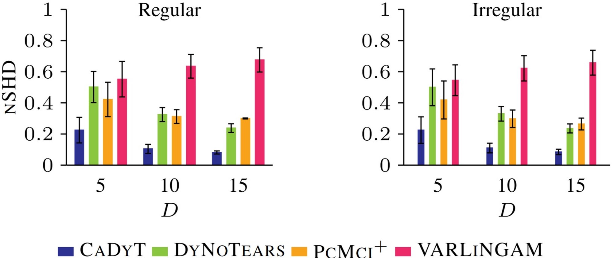
Figure 2: [Lower is better, nSHD ] for random graphs of sizes for regularly sampled data (left) and irregularly sampled data (right). CaDyT finds graphs closer to the ground truth resulting in a lower nSHD.
图 2:随机图规模为 时,规则采样数据(左)与不规则采样数据(右)上的结果。[越低越好,nSHD]。CaDyT 找到的图更接近真实结构,因而 nSHD 更低。
Causal models for time-series
Causal discovery from time-series data has received active research interest over the past decade. Early methods focused on Granger-causality (G-causality) (Granger 1969), which implies that G-causes if including past of helps in predicting the present of . Methods have been designed for both linear (Geweke 1982; Barrett, Barnett, and Seth 2010) and non-linear (Nauta, Bucur, and Seifert 2019) causal models. Methods that are not explicitly based on G-causality lie in the category of constraint-based methods (Chu, Glymour, and Ridgeway 2008; Sun, Taylor, and Bollt 2015; Runge 2020), score-based methods (Pamfil et al. 2020) or noise-based methods (Hyvärinen et al. 2010; Peters, Janzing, and Schölkopf 2013). These methods assume regularly sampled discrete trajectories and overlook the continuous-time structure of time series and the conditions required to reliably learn the underlying dynamics.
面向时间序列的因果模型
过去十年,从时间序列数据中做因果发现一直受到积极关注。早期方法聚焦于 Granger 因果(G-因果)(Granger 1969),其含义是:若加入 的过去有助于预测 的现在,则 G-导致 。人们已经为线性(Geweke 1982;Barrett, Barnett, and Seth 2010)和非线性(Nauta, Bucur, and Seifert 2019)因果模型分别设计了方法。并不显式基于 G-因果的方法,则属于基于约束的方法(Chu, Glymour, and Ridgeway 2008;Sun, Taylor, and Bollt 2015;Runge 2020)、基于分数的方法(Pamfil et al. 2020)或基于噪声的方法(Hyvärinen et al. 2010;Peters, Janzing, and Schölkopf 2013)。这些方法假定轨迹是规则采样的离散序列,忽略了时间序列的连续时间结构,以及可靠学习底层动力学所需的条件。
Voortman, Dash, and Druzdzel (2010) were among the first ones to study under which conditions dynamical systems allow for a causal interpretation, and proposed Difference-based causal models (DBCM). DBCM differ from well known dynamic Bayesian networks in that they force all causation to go through derivatives. This idea was extended by Mooij, Janzing, and Schölkopf (2013) to show that (D)SCMs can model the asymptotic behavior of systems of ODEs with limitations on the possible interventions under DBCM. Those limitations are addressed in recent works (Blom, Bongers, and Mooij 2020; Cinquini et al. 2025).
Voortman, Dash, and Druzdzel(2010)较早研究了在何种条件下动力系统允许因果解释,并提出了基于差分的因果模型(DBCM)。DBCM 与众所周知的动态贝叶斯网的不同之处在于,它们迫使所有因果都经由导数发生。Mooij, Janzing, and Schölkopf(2013)把这一想法加以扩展,表明(D)SCM 可以建模常微分方程组的渐近行为,但在 DBCM 下对可能的干预有限制。这些限制在近期工作中得到讨论(Blom, Bongers, and Mooij 2020;Cinquini et al. 2025)。
Our proposal aims to model a DBCM rather than a dynamic Bayesian network. In contrast to the existing work, our work is uniquely positioned at the intersection of dynamical system learning and causal discovery as it provides a theory-backed approach to modeling the former, while allowing for learning the laws of the process via the latter.
我们的方案旨在建模 DBCM,而不是动态贝叶斯网。与已有工作相比,本文独特地处于动力系统学习与因果发现的交叉处:它为前者提供有理论依据的建模途径,同时又允许通过后者学习过程所遵循的规律。
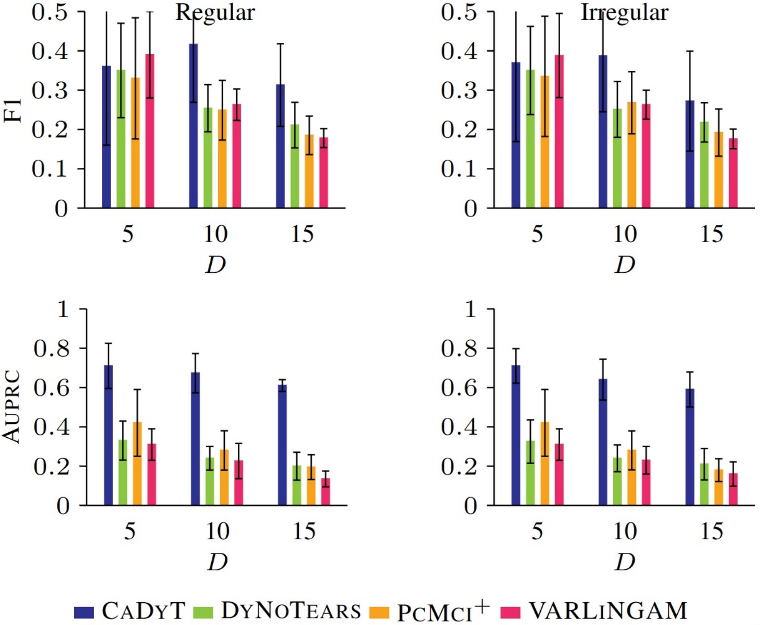
Figure 3: [Higher is better, F1 score (top) and Auprc (bottom)] for random graphs of sizes for regularly (left) resp. irregularly sampled data (right). CaDyT improves over baselines in terms of F1. CaDyT having high Auprc indicates higher confidence about the correct causal edges as opposed to spurious ones.
图 3:随机图规模为 时,规则(左)与不规则(右)采样数据上的结果。[越高越好,F1 分数(上)和 AUPRC(下)]。CaDyT 在 F1 上优于基线。CaDyT 具有较高的 AUPRC,表明它对正确因果边的把握高于虚假边。
6 Experiments
6 实验
Setup
We instantiate CaDyT using parallelized greedy search. We perform our experiments with GPs with RBF-Kernel leveraging explicit Adams-Bashforth (AB) integrators of order . Even though Thm. 1 applies to finite-dimensional Kernels, our choice is motivated by RBF-Kernel’s exact-inference capabilities. Even with over-regularization that could result due to the use of RBF-Kernel, we find that we still outperform the competition. We include the results for CaDyT using Polynomial kernels in the supplementary material. We compare CaDyT with a variety of baselines: The constraint-based (Runge 2020) using non-parametric Kernelized independence test, the score-based DyNoTears (Pamfil et al. 2020), and the noise-based VARLiNGAM (Hyvärinen et al. 2010).
设置
我们用并行化的贪心搜索来实例化 CaDyT。实验使用带 RBF 核的高斯过程,并采用阶数为 的显式 Adams-Bashforth(AB)积分器。尽管定理 1 适用于有限维核,我们的选择仍出于 RBF 核能够精确推断。即便使用 RBF 核可能带来过度正则化,我们仍然发现结果优于对照方法。我们把使用多项式核的 CaDyT 结果放在补充材料中。我们将 CaDyT 与多种基线比较:使用非参数核化独立性检验的基于约束的 (Runge 2020),基于分数的 DyNoTears(Pamfil et al. 2020),以及基于噪声的 VARLiNGAM(Hyvärinen et al. 2010)。
We generate synthetic data using Diamond structure (4 variables) and Erdős–Rényi random graphs with and without cycles for for both regular and irregular timelines. To evaluate the predicted structures we measure the Structural Hamming Distance (SHD) (Tsamardinos, Brown, and Aliferis 2006) which counts the edge mismatch in true and predicted structures. For comparability across structures of different sizes, we normalize SHD between and by dividing with and call this nSHD. To evaluate precision and recall over predicted edges we use the F1 metric, and use Area Under Precision Recall Curve (Auprc) to assess how correct each method is on the edges it is most confident about. We repeat all experiments 20 times with different seeds and report the mean. We report results for the more challenging setting of Erdős–Rényi graphs with both regular and irregular sampling in the manuscript and postpone full experimental details to Appendix B.
我们用钻石结构(4 个变量)以及带环或不带环的 Erdős–Rényi 随机图生成合成数据,规模为 ,时间轴既有规则的也有不规则的。为评估预测出的结构,我们测量结构汉明距离(SHD)(Tsamardinos, Brown, and Aliferis 2006),它统计真实结构与预测结构之间的边不匹配数。为了在不同规模的结构之间可比,我们用 做除法,把 SHD 归一化到 与 之间,并称之为 nSHD。为评估预测边上的精度与召回,我们使用 F1 指标,并用精度-召回曲线下面积(AUPRC)来衡量每种方法对其最有把握的那些边有多正确。所有实验用不同随机种子重复 20 次,并报告均值。我们在正文中报告更具挑战性的设定,即规则与不规则采样下的 Erdős–Rényi 图,完整实验细节放到附录 B。
Results
We perform a sanity check and assess the robustness of CaDyT to false-positives. We generated graphs made of independent ODEs. CaDyT with AB3 never discovered a single spurious edge. Surprisingly, baselines report causal edges for independent data. VARLiNGAM found spurious edges 30% of times, whereas and DyNoTears 60% and 100% respectively.
结果
我们先做一项稳健性检查,评估 CaDyT 对假阳性的稳健程度。我们生成了 10 张由 4 个相互独立的常微分方程组成的图。配合 AB3 的 CaDyT 从未发现任何一条虚假边。出人意料的是,基线却会在独立数据上报告因果边。VARLiNGAM 有 30% 的次数找到虚假边, 和 DyNoTears 则分别为 60% 和 100%。
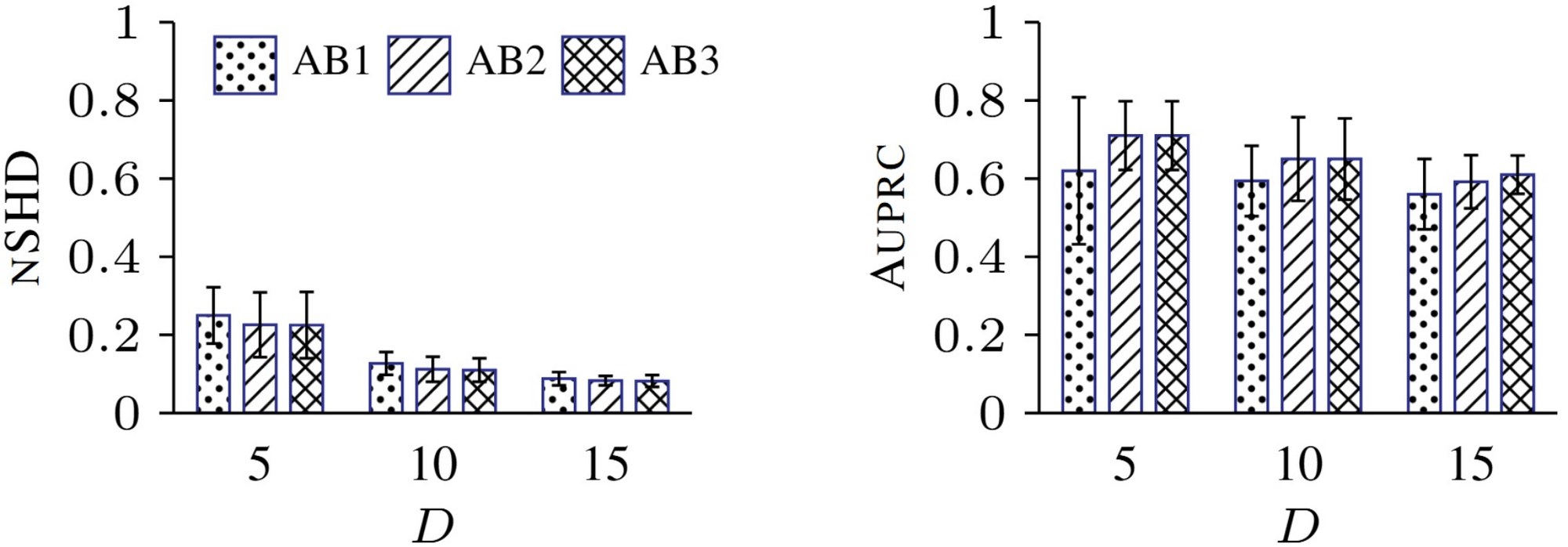
Figure 4: [nSHD (left) Lower is better, Auprc (right) Higher is better] for Adams-Bashforth integrator of order for irregularly sampled data. CaDyT shows gradual improvement with higher order integrators.
图 4:不规则采样数据上,Adams-Bashforth 积分器阶数为 时的结果。[nSHD(左)越低越好,AUPRC(右)越高越好]。CaDyT 随着积分器阶数提高而逐步改进。
Next we sample random dynamical systems and evaluate how well the methods can discover the underlying causal structure. We sample cyclic and acyclic dynamical systems with equal probability and report the results. We report nSHD in Figure n: 2 where we observe that CaDyT consistently outperforms all baselines by a clear margin. Both DyNoTears and demonstrate a high false positive rate which worsens the nSHD. Overall, all methods worsen slightly on irregularly-sampled data, but CaDyT still remains best by a visible margin.
接下来我们采样随机动力系统,评估这些方法能多好地发现底层因果结构。我们以相等概率采样有环与无环的动力系统,并报告结果。我们在图 2 中报告 nSHD,可以看到 CaDyT 始终以明显优势优于所有基线。DyNoTears 和 都表现出较高的假阳性率,从而使 nSHD 变差。总体而言,所有方法在不规则采样数据上都会略差一些,但 CaDyT 仍然明显最好。
To evaluate how well we perform in-terms of precision and recall, we report the F1 score in Figure n: 3. We see that CaDyT is on-par with the baselines for variable sizes , and continues to be robust to false-positives by maintaining a high precision as network size increases. Competing methods on the other hand have very low precision as they tend to predict spurious edges quite frequently.
为评估精度与召回方面的表现,我们在图 3 中报告 F1 分数。可以看到,当变量数为 5 时,CaDyT 与基线相当,并且随着网络变大,它仍能靠较高的精度保持对假阳性的稳健。相比之下,对照方法的精度很低,因为它们往往频繁预测出虚假边。
While nSHD and F1 score could give us a summarized picture of how well the methods perform, we are also interested in how correct are the methods on the causal relationships that they are most confident about. To that end, we calculate the Auprc metric by ordering the predicted edges of each algorithm in decreasing confidence. For CaDyT this confidence is computed using Eq. (18), For we use the p-values associated with each edge whereas for DyNoTears resp. VARLiNGAM we use the strength of the causal edge as present in the predicted adjacency matrix. Looking at the results in Figure n: 3 we see that CaDyT again performs well across benchmarks. A high Auprc indicates that CaDyT is mostly correct about high-confidence edges.
nSHD 和 F1 分数可以概括方法的整体表现,我们还关心:这些方法对它们最有把握的那些因果关系究竟有多正确。为此,我们按置信度降序排列每种算法预测出的边,计算 AUPRC。对 CaDyT,这一置信度用式 (18) 计算;对 ,我们使用每条边对应的 值;对 DyNoTears 和 VARLiNGAM,则使用预测邻接矩阵中该因果边的强度。从图 3 的结果可以看到,CaDyT 再次在各项基准上表现良好。较高的 AUPRC 表明,CaDyT 对高置信度的边大多是正确的。
Effect of Integration Order
To study the effect of the integration scheme, we conduct an ablation study whose result we report in Figure n:4. We compare integrators on irregular timelines and see that higher-order integrators (AB2/AB3) generally outperform AB1. This is consistent with the domain knowledge that higher-order integration schemes approximate the underlying continuous-time dynamics better.
积分阶数的影响
为研究积分方案的影响,我们做了一项消融,结果见图 4。我们在不规则时间轴上比较各积分器,看到高阶积分器(AB2/AB3)通常优于 AB1。这与领域知识一致:高阶积分方案能更好地近似底层的连续时间动力学。
We observed that addition of cycles into the data-generating process affects the methods differently. We find CaDyT tends to improve with the order of integration, where versions leveraging higher-order schemes (AB2 and AB3) stay robust or even improve, whereas the lower-order AB1 variant deteriorates.
我们还观察到,在数据生成过程中加入环,对各方法的影响并不相同。我们发现 CaDyT 往往随积分阶数提高而改进:使用高阶方案(AB2 和 AB3)的版本保持稳健甚至更好,而较低阶的 AB1 变体则会变差。
Oscillators and Chaotic Systems
We further test on the simulated -mass spring system, its analogous real-world counterpart (Schmidt and Lipson 2009), and the hyper-chaotic Rössler Oscillator. To stay fair to the baselines, we use regular sampling. We report results averaged over runs in Table n: 1 which shows that CaDyT outperforms the competing methods and finds causal structures closer to the underlying dynamics (lower SHD), while denoting high confidence about true edges (high Auprc).
振荡器与混沌系统
我们进一步在仿真的二质量弹簧系统、与之类似的真实世界对应物(Schmidt and Lipson 2009),以及超混沌 Rössler 振荡器上测试。为了对基线公平,我们使用规则采样。我们在表 1 中报告 10 次运行的平均结果:CaDyT 优于对照方法,找到的因果结构更接近底层动力学(SHD 更低),同时对真实边有较高把握(AUPRC 更高)。
| Method | DblMass | DblLinear | Rössler |
|---|---|---|---|
| DyNoTears | 0.22 | 0.59 | 0.34 |
| 0.24 | 0.30 | 0.22 | |
| VARLiNGAM | 0.39 | 0.44 | 0.30 |
| CaDyT (ours) | 0.79 | 0.79 | 0.55 |
Table 1: [Higher is better, Auprc ] for the simulated 2-mass spring system (DblMass), for the real double-linear system (DblLinear), and for the Rössler Oscillator (Rössler).
| 方法 | DblMass | DblLinear | Rössler |
|---|---|---|---|
| DyNoTears | 0.22 | 0.59 | 0.34 |
| 0.24 | 0.30 | 0.22 | |
| VARLiNGAM | 0.39 | 0.44 | 0.30 |
| CaDyT(本文) | 0.79 | 0.79 | 0.55 |
表 1:仿真二质量弹簧系统(DblMass)、真实双线性系统(DblLinear)以及 Rössler 振荡器(Rössler)上的结果。[越高越好,AUPRC]。
7 Discussion and Conclusions
7 讨论与结论
We proposed CaDyT , a method for uncovering causal structure in continuous-time dynamics from discrete trajectory data. Our approach combines the exact inference framework of Ensinger et al. (2024) with the Algorithmic Markov Condition (Janzing and Schölkopf 2010). We proved that our score is a valid regularized log-likelihood score (Def.A.2) with an upper-bound asymptotically similar to the BIC, and demonstrated empirically that our score outperforms existing methods. Going forward we see potential lines of improvements as future work.
我们提出了 CaDyT,一种从离散轨迹数据中揭示连续时间动力学因果结构的方法。我们的方法把 Ensinger et al.(2024)的精确推断框架与算法马尔可夫条件(Janzing and Schölkopf 2010)结合起来。我们证明,我们的分数是合法的正则化对数似然分数(定义 A.2),其上界在渐近意义上与 BIC 类似,并在实验中表明该分数优于现有方法。向前看,我们把若干可能的改进列为后续工作。
First, we used greedy graph search and the Adams-Bashforth integrators as the two main components for CaDyT . We do not, however, claim that these to be optimal choices. It is possible that alternate search strategies resp. integrators yield better performance and we aim to investigate such alternative approaches. Second, while using the proposal of Ensinger et al. (2024) allowed us to naturally work with both regular and irregular-sampled trajectories, it has been known to be sensitive to high amount of noise. We conjecture that we could further improve the results by evolving the machinery to be robust to noise. Third, we could extend CaDyT to relax the causal sufficiency assumption by searching for instantaneous edges such that both edge directions give a high score, post backward search. This could potentially point to a hidden confounder. Last, currently CaDyT assumes ODEs can be well-modeled by a GP regression under noisy observation model. A recently proposed extension of DSCMS to chaotic models (Boeken and Mooij 2024) could allow us to relax this assumption further and is a potentially rewarding line of future work.
首先,我们把贪心图搜索和 Adams-Bashforth 积分器作为 CaDyT 的两个主要组成部分,但并不声称这两项选择就是最优的。其他搜索策略或积分器有可能带来更好的表现,我们计划研究这类替代方案。其次,虽然采用 Ensinger et al.(2024)的方案使我们能够自然地同时处理规则与不规则采样轨迹,但已知该方法对大量噪声较为敏感。我们推测,若进一步改进其抗噪声能力,结果还能再提高。第三,我们可以通过搜索瞬时边来放松因果充分假设:若在后向搜索之后,两个方向的边都给出高分,就可能指向隐匿混杂因子。最后,目前 CaDyT 假定常微分方程可以在带噪声观测模型下由高斯过程回归很好地建模。最近把 DSCM 扩展到混沌模型的工作(Boeken and Mooij 2024)或许能让我们进一步放松这一假设,也是一条值得投入的后续方向。
Acknowledgments
致谢
Nicholas Tagliapietra and Katharina Ensinger are supported by Robert Bosch GmbH. Osman Mian is supported by the German Federal Ministry of Research, Technology and Space (DECIPHER-M, 01KD2420C).
Nicholas Tagliapietra 与 Katharina Ensinger 得到 Robert Bosch GmbH 的支持。Osman Mian 得到德国联邦研究、技术与空间部资助(DECIPHER-M,01KD2420C)。
References
参考文献
Barrett, Barnett, and Seth (2010) Barrett, A. B.; Barnett, L.; and Seth, A. K. 2010. Multivariate Granger causality and generalized variance. Physical Review E—Statistical, Nonlinear, and Soft Matter Physics , 81(4).
Bellot, Branson, and van der Schaar (2022) Bellot, A.; Branson, K.; and van der Schaar, M. 2022. Neural graphical modelling in continuous-time: consistency guarantees and algorithms. arXiv:2105.02522.
Blom, Bongers, and Mooij (2020) Blom, T.; Bongers, S.; and Mooij, J. M. 2020. Beyond Structural Causal Models: Causal Constraints Models. In Adams, R. P.; and Gogate, V., eds., Proceedings of The 35th Uncertainty in Artificial Intelligence Conference , volume 115 of PMLR , 585–594. PMLR.
Boeken and Mooij (2024) Boeken, P.; and Mooij, J. M. 2024. Dynamic Structural Causal Models. arXiv:2406.01161.
Brouillard et al. (2020) Brouillard, P.; Lachapelle, S.; Lacoste, A.; Lacoste-Julien, S.; and Drouin, A. 2020. Differentiable causal discovery from interventional data. Advances in Neural Information Processing Systems , 33.
Cavanaugh and Neath (1999) Cavanaugh, J. E.; and Neath, A. A. 1999. Generalizing the derivation of the Schwarz information criterion. Communications in Statistics-Theory and Methods , 28(1).
Chen et al. (2019) Chen, R. T. Q.; Rubanova, Y.; Bettencourt, J.; and Duvenaud, D. 2019. Neural Ordinary Differential Equations. arXiv:1806.07366.
Chickering (2002) Chickering, D. M. 2002. Optimal structure identification with greedy search. JMLR , 3.
Chu, Glymour, and Ridgeway (2008) Chu, T.; Glymour, C.; and Ridgeway, G. 2008. Search for Additive Nonlinear Time Series Causal Models. Journal of Machine Learning Research , 9(5).
Cinquini et al. (2025) Cinquini, M.; Beretta, I.; Ruggieri, S.; and Valera, I. 2025. A Practical Approach to Causal Inference over Time. Proceedings of the AAAI Conference on Artificial Intelligence , 39: 14832–14839.
Claeskens and Hjort (2008) Claeskens, G.; and Hjort, N. L. 2008. Model selection and model averaging. Cambridge books .
Deisenroth and Rasmussen (2011) Deisenroth, M. P.; and Rasmussen, C. E. 2011. PILCO: a model-based and data-efficient approach to policy search. In Proceedings of the 28th ICML , ICML’11. Omnipress.
Ensinger et al. (2024) Ensinger, K.; Tagliapietra, N.; Ziesche, S.; and Trimpe, S. 2024. Exact inference for continuous-time Gaussian process dynamics. In Proceedings of the Thirty-Eighth AAAI Conference on Artificial Intelligence and Thirty-Sixth Conference on Innovative Applications of Artificial Intelligence and Fourteenth Symposium on Educational Advances in Artificial Intelligence , AAAI’24/IAAI’24/EAAI’24. AAAI Press.
Geweke (1982) Geweke, J. 1982. Measurement of linear dependence and feedback between multiple time series. Journal of the American statistical association , 77(378).
Glass, Ensinger, and Zimmer (2024) Glass, L.; Ensinger, K.; and Zimmer, C. 2024. Safe Active Learning for Gaussian Differential Equations. arXiv:2412.09053.
Granger (1969) Granger, C. W. J. 1969. Investigating Causal Relations by Econometric Models and Cross-spectral Methods. Econometrica , 37(3): 424–438.
Grunwald (2004) Grunwald, P. 2004. A tutorial introduction to the minimum description length principle. arXiv:math/0406077.
Grünwald (2007) Grünwald, P. D. 2007. The minimum description length principle . MIT press.
Hairer, Nørsett, and Wanner (2008) Hairer, E.; Nørsett, S.; and Wanner, G. 2008. Solving Ordinary Differential Equations I: Nonstiff Problems . Springer Series in Computational Mathematics. Springer Berlin Heidelberg. ISBN 9783540566700.
Haughton (1988) Haughton, D. M. 1988. On the choice of a model to fit data from an exponential family. The annals of statistics .
Hedge et al. (2022) Hedge, P.; Yildiz, C.; Lähdesmäki, H.; Kaski, S.; and Heinonen, M. 2022. Variational multiple shooting for Bayesian ODEs with Gaussian processes. In Proceedings of the 38th Conference on Uncertainty in Artificial Intelligence (UAI 2022), PMLR , Proceedings of Machine Learning Research, 790–799. United States: JMLR. Conference on Uncertainty in Artificial Intelligence, UAI ; Conference date: 01-08-2022 Through 05-08-2022.
Heinonen et al. (2018) Heinonen, M.; Yildiz, C.; Mannerström, H.; Intosalmi, J.; and Lähdesmäki, H. 2018. Learning unknown ODE models with Gaussian processes. In Proceedings of the 35th ICML, ICML 2018 , volume 5 of PMLR , 3120–3132. United States: International Machine Learning Society.
Hoyer et al. (2009) Hoyer, P.; Janzing, D.; Mooij, J. M.; Peters, J.; and Schölkopf, B. 2009. Nonlinear causal discovery with additive noise models. In NeurIPS , volume 21. Curran.
Huang et al. (2018) Huang, B.; Zhang, K.; Lin, Y.; Schölkopf, B.; and Glymour, C. 2018. Generalized score functions for causal discovery. In ACM SIGKDD .
Hyvärinen et al. (2010) Hyvärinen, A.; Zhang, K.; Shimizu, S.; and Hoyer, P. O. 2010. Estimation of a structural vector autoregression model using non-Gaussianity. Journal of Machine Learning Research , 11(5).
Janzing and Schölkopf (2010) Janzing, D.; and Schölkopf, B. 2010. Causal inference using the Algorithmic Markov Condition. IEEETPAMI , 56: 5168–5194.
Kakade, Seeger, and Foster (2005) Kakade, S. M.; Seeger, M. W.; and Foster, D. P. 2005. Worst-Case Bounds for Gaussian Process Models. In Weiss, Y.; Schölkopf, B.; and Platt, J., eds., NeurIPS , volume 18. MIT Press.
Kaltenpoth and Vreeken (2019) Kaltenpoth, D.; and Vreeken, J. 2019. We Are Not Your Real Parents: Telling Causal from Confounded by MDL. In SDM . SIAM.
Kashyap (1982) Kashyap, R. L. 1982. Optimal choice of AR and MA parts in autoregressive moving average models. IEEE Transactions on Pattern Analysis and Machine Intelligence , 2.
Kass and Raftery (1995) Kass, R. E.; and Raftery, A. E. 1995. Bayes factors. Journal of the american statistical association , 90(430).
Kolmogorov (1965) Kolmogorov, A. N. 1965. Three approaches to the quantitative definition ofinformation’. Problems of information transmission , 1(1).
Kraft (1949) Kraft, L. G. 1949. A device for quantizing, grouping, and coding amplitude-modulated pulses . Ph.D. thesis, Massachusetts Institute of Technology.
Lu, Zhang, and Yuan (2021) Lu, N. Y.; Zhang, K.; and Yuan, C. 2021. Improving causal discovery by optimal bayesian network learning. In Proceedings of the AAAI Conference on Artificial Intelligence , volume 35.
Mameche, Kaltenpoth, and Vreeken (2023) Mameche, S.; Kaltenpoth, D.; and Vreeken, J. 2023. Learning Causal Models under Independent Changes. In Oh, A.; Naumann, T.; Globerson, A.; Saenko, K.; Hardt, M.; and Levine, S., eds., Advances in Neural Information Processing Systems , volume 36, 75595–75622. Curran Associates, Inc.
Martin, Buhmann, and Ablowitz (2003) Martin, B.; Buhmann, M.; and Ablowitz, J. 2003. Radial basis functions: theory and implementations. Cambridge University (ISBN: 0-521-63338-9.) .
Marx and Vreeken (2019a) Marx, A.; and Vreeken, J. 2019a. Identifiability of Cause and Effect using Regularized Regression. In KDD . ACM.
Marx and Vreeken (2019b) Marx, A.; and Vreeken, J. 2019b. Telling cause from effect by local and global regression. KAIS , 60(3): 1277–1305.
Marx and Vreeken (2021) Marx, A.; and Vreeken, J. 2021. Formally Justifying MDL-based Inference of Cause and Effect. arXiv:2105.01902.
Mian, Marx, and Vreeken (2021) Mian, O.; Marx, A.; and Vreeken, J. 2021. Discovering Fully Oriented Causal Networks. In AAAI .
Mogensen and Hansen (2020) Mogensen, S. W.; and Hansen, N. R. 2020. Markov equivalence of marginalized local independence graphs. The Annals of Statistics , 48(1).
Mooij, Janzing, and Schölkopf (2013) Mooij, J. M.; Janzing, D.; and Schölkopf, B. 2013. From ordinary differential equations to structural causal models: the deterministic case. arXiv preprint arXiv:1304.7920 .
Nauta, Bucur, and Seifert (2019) Nauta, M.; Bucur, D.; and Seifert, C. 2019. Causal discovery with attention-based convolutional neural networks. Machine Learning and Knowledge Extraction , 1(1).
Pamfil et al. (2020) Pamfil, R.; Sriwattanaworachai, N.; Desai, S.; Pilgerstorfer, P.; Georgatzis, K.; Beaumont, P.; and Aragam, B. 2020. Dynotears: Structure learning from time-series data. In International Conference on Artificial Intelligence and Statistics . Pmlr.
Pearl (2009) Pearl, J. 2009. Causality . Cambridge university press.
Peters, Janzing, and Schölkopf (2013) Peters, J.; Janzing, D.; and Schölkopf, B. 2013. Causal inference on time series using restricted structural equation models. Advances in neural information processing systems , 26.
Rahimi and Recht (2007) Rahimi, A.; and Recht, B. 2007. Random features for large-scale kernel machines. Advances in neural information processing systems , 20.
Ramsey et al. (2010) Ramsey, J. D.; Hanson, S. J.; Hanson, C.; Halchenko, Y. O.; Poldrack, R. A.; and Glymour, C. 2010. Six problems for causal inference from fMRI. neuroimage , 49(2).
Rasmussen and Williams (2005) Rasmussen, C. E.; and Williams, C. K. I. 2005. Gaussian Processes for Machine Learning (Adaptive Computation and Machine Learning) . The MIT Press.
Ridderbusch, Ober-Blöbaum, and Goulart (2023) Ridderbusch, S.; Ober-Blöbaum, S.; and Goulart, P. 2023. The past does matter: correlation of subsequent states in trajectory predictions of Gaussian Process models. In Uncertainty in Artificial Intelligence, UAI 2023, July 31 - 4 August 2023, Pittsburgh, PA, USA , volume 216, 1752–1761. PMLR.
Rissanen (1983) Rissanen, J. 1983. A Universal Prior for Integers and Estimation by Minimum Description Length. AnnalsStatistics , 11(2): 416–431.
Rubenstein et al. (2016) Rubenstein, P. K.; Bongers, S.; Schölkopf, B.; and Mooij, J. M. 2016. From deterministic ODEs to dynamic structural causal models. arXiv preprint arXiv:1608.08028 .
Runge (2020) Runge, J. 2020. Discovering contemporaneous and lagged causal relations in autocorrelated nonlinear time series datasets. In Conference on uncertainty in artificial intelligence . Pmlr.
Rössler (1976) Rössler, O. 1976. An equation for continuous chaos. Physics Letters A , 57(5): 397–398.
Schmidt and Lipson (2009) Schmidt, M.; and Lipson, H. 2009. Distilling Free-Form Natural Laws from Experimental Data. Science , 324(5923).
Schwarz (1978) Schwarz, G. 1978. Estimating the dimension of a model. The annals of statistics .
Strogatz (2000) Strogatz, S. H. 2000. Nonlinear Dynamics and Chaos: With Applications to Physics, Biology, Chemistry and Engineering . Westview Press.
Sun, Taylor, and Bollt (2015) Sun, J.; Taylor, D.; and Bollt, E. M. 2015. Causal network inference by optimal causation entropy. SIAM Journal on Applied Dynamical Systems , 14(1).
Tsamardinos, Brown, and Aliferis (2006) Tsamardinos, I.; Brown, L. E.; and Aliferis, C. F. 2006. The max-min hill-climbing Bayesian network structure learning algorithm. Machine Learning , 65.
Van der Vaart (2000) Van der Vaart, A. W. 2000. Asymptotic statistics , volume 3. Cambridge university press.
Vereshchagin and Vitányi (2004) Vereshchagin, N. K.; and Vitányi, P. M. 2004. Kolmogorov’s structure functions and model selection. IEEETIT , 50(12).
Voortman, Dash, and Druzdzel (2010) Voortman, M.; Dash, D.; and Druzdzel, M. J. 2010. Learning causal models that make correct manipulation predictions with time series data. In Causality: Objectives and Assessment . PMLR.
Wang, Fleet, and Hertzmann (2005) Wang, J. M.; Fleet, D. J.; and Hertzmann, A. 2005. Gaussian Process Dynamical Models. In NeurIPS 2005 . Cambridge, MA, USA: MIT Press.
Wang et al. (2017) Wang, Y.; Solus, L.; Yang, K. D.; and Uhler, C. 2017. Permutation-based Causal Inference Algorithms with Interventions. In NIPS .
Wendland (1995) Wendland, H. 1995. Piecewise polynomial, positive definite and compactly supported radial functions of minimal degree. Advances in computational Mathematics , 4(1).
Williams and Seeger (2000) Williams, C.; and Seeger, M. 2000. Using the Nyström method to speed up kernel machines. Advances in neural information processing systems , 13.
Xu, Mameche, and Vreeken (2025) Xu, S.; Mameche, S.; and Vreeken, J. 2025. Information-Theoretic Causal Discovery in Topological Order. In AISTATS 2025 .
Xu et al. (2022) Xu, S.; Mian, O. A.; Marx, A.; and Vreeken, J. 2022. Inferring cause and effect in the presence of heteroscedastic noise. In ICML . PMLR.
Reproducibility Checklist
可复现性清单
Instructions for Authors:
致作者的说明:
This document outlines key aspects for assessing reproducibility. Please provide your input by editing this .tex file directly.
本文件列出评估可复现性的关键方面。请直接编辑本 .tex 文件填写。
For each question (that applies), replace the “Type your response here” text with your answer.
对每个(适用的)问题,请把 “Type your response here” 替换为你的答案。
Example: If a question appears as
示例: 若某个问题显示为
\question{Proofs of all novel claims are included} {(yes/partial/no)} Type your response here
you would change it to:
则应改为:
\question{Proofs of all novel claims are included} {(yes/partial/no)} yes
Please make sure to:
请务必:
- • Replace ONLY the “Type your response here” text and nothing else.
- • 只替换 “Type your response here” 这一处文字,不要改动其他内容。
- • Use one of the options listed for that question (e.g., yes, no, partial, or NA).
- • 使用该问题列出的选项之一(例如 yes、no、partial 或 NA)。
- • Not modify any other part of the \question command or any other lines in this document.
- • 不要修改 \question 命令的其他部分,也不要改动本文档中的其他行。
You can \input this .tex file right before \end{document} of your main file or compile it as a stand-alone document. Check the instructions on your conference’s website to see if you will be asked to provide this checklist with your paper or separately.
你可以把本 .tex 文件用 \input 放在主文件的 \end{document} 之前,也可以把它编译成独立文档。请查看所投会议网站上的说明,确认这份清单是随论文一并提交,还是单独提交。
1. General Paper Structure
- 1.1. Includes a conceptual outline and/or pseudocode description of AI methods introduced (yes/partial/no/NA) yes
1. 论文总体结构
- 1.1. 对文中引入的人工智能方法,是否包含概念性提纲和/或伪代码说明(yes/partial/no/NA) yes
- 1.2. Clearly delineates statements that are opinions, hypothesis, and speculation from objective facts and results (yes/no) yes
- 1.2. 是否把意见、假设和推测与客观事实及结果清楚分开(yes/no) yes
- 1.3. Provides well-marked pedagogical references for less-familiar readers to gain background necessary to replicate the paper (yes/no) yes
- 1.3. 是否为较不熟悉该领域的读者提供了标注清楚的教学性参考文献,以便获得复现论文所需的背景(yes/no) yes
2. Theoretical Contributions
- 2.1. Does this paper make theoretical contributions? (yes/no) yes If yes, please address the following points: 2.2. All assumptions and restrictions are stated clearly and formally (yes/partial/no) yes 2.3. All novel claims are stated formally (e.g., in theorem statements) (yes/partial/no) yes 2.4. Proofs of all novel claims are included (yes/partial/no) yes 2.5. Proof sketches or intuitions are given for complex and/or novel results (yes/partial/no) yes 2.6. Appropriate citations to theoretical tools used are given (yes/partial/no) yes 2.7. All theoretical claims are demonstrated empirically to hold (yes/partial/no/NA) partial 2.8. All experimental code used to eliminate or disprove claims is included (yes/no/NA) yes
2. 理论贡献
- 2.1. 本文是否作出理论贡献?(yes/no) yes 若是,请回答以下几点: 2.2. 所有假设与限制是否陈述清楚且形式化(yes/partial/no) yes 2.3. 所有新主张是否形式化陈述(例如写在定理中)(yes/partial/no) yes 2.4. 是否包含所有新主张的证明(yes/partial/no) yes 2.5. 对复杂和/或新的结果,是否给出证明梗概或直观说明(yes/partial/no) yes 2.6. 对所用理论工具是否给出适当引用(yes/partial/no) yes 2.7. 所有理论主张是否都用实验表明成立(yes/partial/no/NA) partial 2.8. 用于排除或反驳主张的全部实验代码是否包含在内(yes/no/NA) yes
3. Dataset Usage
- 3.1. Does this paper rely on one or more datasets? (yes/no) yes If yes, please address the following points: 3.2. A motivation is given for why the experiments are conducted on the selected datasets (yes/partial/no/NA) yes 3.3. All novel datasets introduced in this paper are included in a data appendix (yes/partial/no/NA) yes 3.4. All novel datasets introduced in this paper will be made publicly available upon publication of the paper with a license that allows free usage for research purposes (yes/partial/no/NA) yes 3.5. All datasets drawn from the existing literature (potentially including authors’ own previously published work) are accompanied by appropriate citations (yes/no/NA) NA 3.6. All datasets drawn from the existing literature (potentially including authors’ own previously published work) are publicly available (yes/partial/no/NA) NA 3.7. All datasets that are not publicly available are described in detail, with explanation why publicly available alternatives are not scientifically satisficing (yes/partial/no/NA) NA
3. 数据集使用
- 3.1. 本文是否依赖一个或多个数据集?(yes/no) yes 若是,请回答以下几点: 3.2. 是否说明为何在所选数据集上做实验(yes/partial/no/NA) yes 3.3. 本文新引入的全部数据集是否放在数据附录中(yes/partial/no/NA) yes 3.4. 本文新引入的全部数据集是否将在论文发表后公开,并配有允许免费用于研究的许可证(yes/partial/no/NA) yes 3.5. 来自已有文献(可能包括作者此前已发表工作)的全部数据集是否附有适当引用(yes/no/NA) NA 3.6. 来自已有文献(可能包括作者此前已发表工作)的全部数据集是否公开可得(yes/partial/no/NA) NA 3.7. 所有非公开数据集是否有详细描述,并说明为何公开的替代数据在科学上不够满足需求(yes/partial/no/NA) NA
4. Computational Experiments
- 4.1. Does this paper include computational experiments? (yes/no) yes If yes, please address the following points: 4.2. This paper states the number and range of values tried per (hyper-) parameter during development of the paper, along with the criterion used for selecting the final parameter setting (yes/partial/no/NA) yes 4.3. Any code required for pre-processing data is included in the appendix (yes/partial/no) yes 4.4. All source code required for conducting and analyzing the experiments is included in a code appendix (yes/partial/no) yes 4.5. All source code required for conducting and analyzing the experiments will be made publicly available upon publication of the paper with a license that allows free usage for research purposes (yes/partial/no) yes 4.6. All source code implementing new methods have comments detailing the implementation, with references to the paper where each step comes from (yes/partial/no) partial 4.7. If an algorithm depends on randomness, then the method used for setting seeds is described in a way sufficient to allow replication of results (yes/partial/no/NA) yes 4.8. This paper specifies the computing infrastructure used for running experiments (hardware and software), including GPU/CPU models; amount of memory; operating system; names and versions of relevant software libraries and frameworks (yes/partial/no) yes 4.9. This paper formally describes evaluation metrics used and explains the motivation for choosing these metrics (yes/partial/no) yes 4.10. This paper states the number of algorithm runs used to compute each reported result (yes/no) yes 4.11. Analysis of experiments goes beyond single-dimensional summaries of performance (e.g., average; median) to include measures of variation, confidence, or other distributional information (yes/no) yes 4.12. The significance of any improvement or decrease in performance is judged using appropriate statistical tests (e.g., Wilcoxon signed-rank) (yes/partial/no) yes 4.13. This paper lists all final (hyper-)parameters used for each model/algorithm in the paper’s experiments (yes/partial/no/NA) partial
4. 计算实验
- 4.1. 本文是否包含计算实验?(yes/no) yes 若是,请回答以下几点: 4.2. 本文是否说明在论文开发过程中每个(超)参数尝试过的取值数量与范围,以及选择最终参数设置的准则(yes/partial/no/NA) yes 4.3. 数据预处理所需的任何代码是否包含在附录中(yes/partial/no) yes 4.4. 开展和分析实验所需的全部源代码是否包含在代码附录中(yes/partial/no) yes 4.5. 开展和分析实验所需的全部源代码是否将在论文发表后公开,并配有允许免费用于研究的许可证(yes/partial/no) yes 4.6. 实现新方法的全部源代码是否有注释说明实现细节,并引用论文中对应步骤(yes/partial/no) partial 4.7. 若算法依赖于随机性,设置种子的方法是否描述得足以复现结果(yes/partial/no/NA) yes 4.8. 本文是否说明运行实验所用的计算基础设施(硬件与软件),包括 GPU/CPU 型号、内存容量、操作系统,以及相关软件库与框架的名称和版本(yes/partial/no) yes 4.9. 本文是否形式化描述所用评估指标,并解释选择这些指标的动机(yes/partial/no) yes 4.10. 本文是否说明计算每项报告结果所用的算法运行次数(yes/no) yes 4.11. 实验分析是否超越表现的单维摘要(例如均值、中位数),而包含变异、置信或其他分布信息(yes/no) yes 4.12. 任何表现提升或下降的显著性是否用适当的统计检验来判断(例如 Wilcoxon 符号秩检验)(yes/partial/no) yes 4.13. 本文是否列出论文实验中每个模型/算法所用的全部最终(超)参数(yes/partial/no/NA) partial
Appendix A Theoretical Results
附录 A 理论结果
In this section we provide proofs for our theoretical results. For ease of recall, we restate Assumptions. 1,2 and Theorem. 1 below along with the definitions of regularized log-likelihood scores and specifically the BIC score (Schwarz 1978).
本节给出理论结果的证明。为便于对照,我们在下面重述假设 1、2 和定理 1,并给出正则化对数似然分数、特别是 BIC 分数(Schwarz 1978)的定义。
Definition A.1(Bayesian Information Criterion).
For a statistical model with free parameters and maximum log-likelihood , the Bayesian Information Criterion (BIC) is defined as
定义 A.1(贝叶斯信息准则)。
对具有 个自由参数、最大对数似然为 的统计模型 ,贝叶斯信息准则(BIC)定义为
where is the number of observations. Lower values of indicate a preferred model under an asymptotic approximation to the Bayes factor (Schwarz 1978). For a Gaussian likelihood with residual sum of squares , this further simplifies to
其中 是观测数。较低的 值表示,在对贝叶斯因子的渐近近似下,该模型更受偏好(Schwarz 1978)。对具有残差平方和 的高斯似然,这进一步简化为
with generalized BIC taking the form
广义 BIC 则取如下形式
with and as constant terms independent of (Ramsey et al. 2010, Appendix. A).
其中 与 是与 无关的常数项(Ramsey et al. 2010,附录 A)。
In the following we focus on an arbitrary submodel. We partially skip indices identifying the specific submodel where unnecessary.
下面我们聚焦于任意一个子模型。在不必标明的地方,我们部分省略用来识别具体子模型的下标。
Definition A.2(Regularized log-likelihood score).
Given observations, an empirical estimate of residual noise variance, , and model dependent constants independent of , we define a regularized log-likelihood score
定义 A.2(正则化对数似然分数)。
给定 个观测、残差噪声方差的经验估计 ,以及与模型有关、但与 无关的常数 ,我们定义正则化对数似然分数
with a function that fullfills .
其中 是满足 的函数。
Assumption 1(Finite dimensions).
is finite-dimensional.
假设 1(有限维)。
是有限维的。
Assumption 2(Bounded hyperparameters and precision).
The lengtscale parameter , the variance parameter are upper bounded. All precisions within each model are upper bounded.
假设 2(超参数与精度有界)。
长度尺度参数 、方差参数 有上界。每个模型 内的全部精度 有上界。
Lemma 1.
Given a DSCM , let be a trajectory generated from and let . If Assms. 1,2 hold, it holds asymptotically
引理 1。
给定 DSCM ,设 是由 生成的一条轨迹,并令 。若假设 1、2 成立,则渐近地有
\bar{L}(\mathcal{T},M_{j})\leq c_{0}\cdot N\cdot log(\hat{\sigma}_{\color[rgb]{0.75,0,0.25}{j}}^{2})+c_{1}^{(j)}log(N)+c_{2}^{(j)}.
with constants independent of .
其中常数 与 无关。
Proof.
Recall that we formally define as:
证明。
回顾我们把 形式化定义为:
Specifically, whenever we subtract from subsequent expressions, we subtract the first term from Eq. (15), second term from Eq. (16) and the last term from Eq. (17) contained in those expressions. We equivalently obtain,
具体而言,每当我们从后续表达式中减去 时,减去的是这些表达式里式 (15) 的第一项、式 (16) 的第二项以及式 (17) 的最后一项。我们等价地得到,
with resp. defined formally as,
其中 与 分别形式化定义为,
where and .
其中 ,。
We begin by looking at the remaining term in Eq. (17) we observe that it can be rewritten as
我们先看法 (17) 中剩下的项,可以看到它可以改写为
where the constant is independent of the submodel.
其中常数 与子模型无关。
Next, we analyze the local model cost and show that it does not grow faster than the likelihood term in Eq.(17).
接下来,我们分析局部模型成本 ,并表明它的增长不快于式 (17) 中的似然项。
For local models it holds that
对局部模型,有
as these two terms are independent of . This leaves us with Eq. (16) without the term that we excluded from to get where we omit the submodel index for ease of notation:
因为这两项与 无关。这样我们就只剩下去掉 项后的式 (16)——该项已从 中排除以得到 ——为书写方便,我们省略子模型下标 :
Referring to eigenvalues as with size and using the notation for length scales and variances, for their number, let with size be the set of values assigned to each eigenvalue and parameter. Letting , we have,
把特征值记为 ,其个数为 ,并用记号 表示长度尺度与方差, 表示它们的个数。令 为赋给每个特征值与参数的取值集合,其大小 。设 ,则有,
where we transition from Eq. (A.10) to Eq. (A.11) by using the inequality for all , which is always the case for us as we would use with atleast . Eq. (A.15) implies that the complexity of is upper bounded by the complexity of the log determinant term of the learned Kernel matrix . To evaluate this complexity, we include the result of Kakade, Seeger, and Foster (2005, Sec 3.2) which states that for Kernels with finite dimensions (ref. Assm 1) we have,
其中我们从式 (A.10) 过渡到式 (A.11) 时,使用了不等式 (对所有 ),而这在我们这里总是成立的,因为我们使用 时至少取 。式 (A.15) 意味着 的复杂度以上界受所学核矩阵 的对数行列式项复杂度控制。为评估这一复杂度,我们引入 Kakade, Seeger, and Foster(2005,第 3.2 节)的结果:对有限维核(参见假设 1),有
Substituting this into Eq. (A.15) and re-introducing the submodel index , we get
把它代入式 (A.15) 并重新引入子模型下标 ,得到
This means
这意味着
Combining Eq. (A.4), Eq. (A.5) and Eq. (A.17) we get
把式 (A.4)、式 (A.5) 和式 (A.17) 合在一起,得到
Note that the second term is in which means that the upper bound of the parameter penalty grows sublinearly in whereas the likelihood term scales in and dominates in the limit, giving us a valid regularized log-likelihood score. ∎
注意第二项属于 ,这意味着参数惩罚的上界随 次线性增长,而似然项按 尺度增长,并在极限中占主导,从而使我们得到合法的正则化对数似然分数。∎
Theorem 2.
Given a DSCM , let be a trajectory generated from and let . If Assms. 1,2 hold, it holds asymptotically.
定理 2。
给定 DSCM ,设 是由 生成的一条轨迹,并令 。若假设 1、2 成立,则渐近地有
with constants and independent of and asymptotically is a valid regularized log-likelihood score according to Definition A.2.
其中常数 和 与 无关,并且按照定义 A.2, 在渐近意义上是合法的正则化对数似然分数。
Proof.
We first split into two sums as formalized in the proof of Lemm. 1,
证明。
我们先按引理 1 的证明中的写法,把 拆成两个求和,
Next we consider these two terms individually. Note that we can expand the first term as
接下来分别考虑这两项。注意第一项可以展开为
We expand the second term similarly,
我们用类似方式展开第二项,
with where we combine the sum into the constant and .
其中我们把求和 合并成常数 ,并令 。
Putting together the two results we get,
把两项结果合在一起,得到,
∎
Corollary 3.
Model selection using is equivalent to model selection using .
推论 3。
用 做模型选择,等价于用 做模型选择。
Proof.
Note that even though contains terms in i.e. (Eq.(15)) and in Eq. (16) we have , these terms remain constant across models fitted on same length . The same holds for the terms and .Therefore, they do not influence the model being learned. Hence, the term of Eq.(15), and and cancel out when comparing two models using and do not affect the score change and do not change the model selection process. ∎
证明。
注意,尽管 包含 量级的项,即 (式 (15)),并且在式 (16) 中有 ,但这些项在拟合于同一长度 的模型之间保持不变。对项 以及 也是如此。因此,它们并不影响正在学习的模型。于是,在用 比较两个模型时,式 (15) 的 项、、 以及 会相互抵消,既不影响分数变化,也不改变模型选择过程。∎
Regularized log-likelihood scores have been widely used to establish consistency (Huang et al. 2018; Marx and Vreeken 2019a; Brouillard et al. 2020; Mian, Marx, and Vreeken 2021; Xu et al. 2022; Xu, Mameche, and Vreeken 2025). Both the Bayesian Information Criterion (BIC) and its generalization introduced in Def. A.1 can be viewed as special cases of regularized log-likelihood scores. These criteria are well established for independent and identically distributed (i.i.d.) data; see, e.g., (Van der Vaart 2000, Sec. 5.5), (Kashyap 1982; Haughton 1988; Kass and Raftery 1995; Chickering 2002; Marx and Vreeken 2019a; Lu, Zhang, and Yuan 2021; Mian, Marx, and Vreeken 2021). For BIC-type scores, consistency guarantees have been shown to extend to non-i.i.d. time-series data under the following conditions:
正则化对数似然分数已被广泛用于建立一致性(Huang et al. 2018;Marx and Vreeken 2019a;Brouillard et al. 2020;Mian, Marx, and Vreeken 2021;Xu et al. 2022;Xu, Mameche, and Vreeken 2025)。贝叶斯信息准则(BIC)及其在定义 A.1 中引入的推广,都可以看成正则化对数似然分数的特例。这些准则在独立同分布(i.i.d.)数据上已经有很好的基础;参见例如 (Van der Vaart 2000,第 5.5 节),(Kashyap 1982;Haughton 1988;Kass and Raftery 1995;Chickering 2002;Marx and Vreeken 2019a;Lu, Zhang, and Yuan 2021;Mian, Marx, and Vreeken 2021)。对 BIC 类分数,一致性保证在下列条件下已被表明可以延伸到非独立同分布的时间序列数据:
i. The likelihood term satisfies mild regularity conditions (Cavanaugh and Neath 1999, Sec. 3).
i. 似然项满足温和的正则条件(Cavanaugh and Neath 1999,第 3 节)。
ii. The true model is contained in the candidate model set, and the number of models does not grow with (Claeskens and Hjort 2008, Thm 4.2).
ii. 真实模型包含在候选模型集合中,并且模型个数不随 增长(Claeskens and Hjort 2008,定理 4.2)。
Condition i. involves standard assumptions such as twice continuous differentiability of the likelihood function with respect to its parameters, which typically holds for Gaussian process regression. Condition ii. follows directly from causal sufficiency and Assumption 1 in our setting. The form of regularized log-likelihood scores we describe is general, and our particular instantiation represents one specific case within this broader class. Most of the cited works analyze alternative forms of regularized log-likelihoods and establish convergence results. Because our score includes a term of the form plus a correction term, we are optimistic that convergence guarantees or selection of the correct model up to precision can be formally shown in future work.
条件 i. 涉及一些标准假设,例如似然函数对其参数二次连续可微,这对高斯过程回归通常成立。条件 ii. 在我们的设定下由因果充分性与假设 1 直接得到。我们所描述的正则化对数似然分数形式是一般性的,本文的具体实例化只是这一更广类别中的一种情形。多数被引工作分析的是其他形式的正则化对数似然,并建立了收敛结果。由于我们的分数包含 项再加上一个修正项,我们有理由期待,收敛保证、或在精度 下选择正确模型,可以在后续工作中被形式化证明。
Appendix B Benchmarks Details
附录 B 基准细节
Hereby, we provide further details on our experimental setting.
在此,我们补充实验设置的进一步细节。
Computational Resources
计算资源
All our results are efficiently run by parallelizing the greedy search on a AMD EPYC 7643 CPU with 60GB RAM allocated.
我们的全部结果都通过在 AMD EPYC 7643 CPU 上并行化贪心搜索高效完成,分配内存为 60GB。
Physical Models
物理模型
We provide a detailed description for each benchmark, including the underlying physical models and their initial conditions. Each dynamics described below has been integrated using , after which an additive gaussian noise has been applied.
我们对每个基准给出详细描述,包括底层物理模型及其初值。下面描述的每套动力学都用 积分,之后再加入加性高斯噪声 。
Empty Causal Graph:
For the empty causal graph, we generate independent trajectories using ODEs that do not have any inter-dependency. Those ODEs are in the form with . Those ODEs result in either an exponential growth or decay. The timeline of integration is with , what has been tested with regular and irregular timelines. The additive nosie std. is .
空因果图:
对空因果图,我们用 个彼此没有相互依赖的常微分方程生成 条独立轨迹。这些方程形如 ,其中 。它们会带来指数增长或衰减。积分时间轴为 ,,并在规则时间轴以及不规则()时间轴上做了测试。加性噪声的标准差为 。
Diamond Causal Graph:
We test on the Diamond Causal Graph, which represents a simple benchmark containing all the basic causal structures: The fork, the mediator, and the collider. Below, we provide an illustration.
钻石因果图:
我们在钻石因果图上测试,它是一个简单基准,包含全部基本因果结构:分叉、中介和对撞。下面给出示意图。
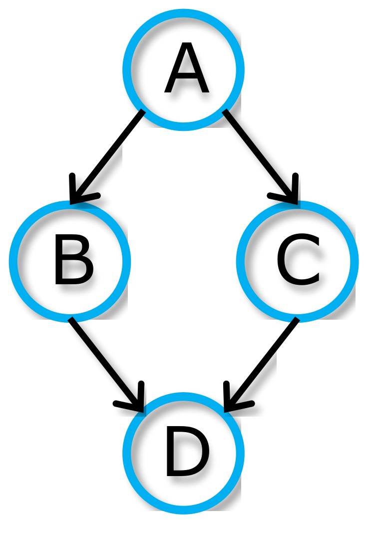
$$\begin{aligned} \frac{dA}{dt}&=\dfrac{1}{2}\cdot\sin{(t)}\
\frac{dB}{dt}&=\dfrac{1}{2}\cdot\sin{(A)}\
\frac{dC}{dt}&=-2\cdot\cos{(A)}\
\frac{dD}{dt}&=B+C\
\end{aligned} \tag{A.19}$$
钻石因果图及对应的常微分方程组:
$$\begin{aligned} \frac{dA}{dt}&=\dfrac{1}{2}\cdot\sin{(t)}\
\frac{dB}{dt}&=\dfrac{1}{2}\cdot\sin{(A)}\
\frac{dC}{dt}&=-2\cdot\cos{(A)}\
\frac{dD}{dt}&=B+C\
\end{aligned} \tag{A.19}$$
The initial conditions are randomly sampled from a gaussian distribution with and . The timeline of integration is and . We tested on both a regular and irregular () timeline. For the Diamond, the additive noise std. is .
初值从均值为 、标准差为 的高斯分布中随机采样。积分时间轴为 ,。我们在规则时间轴和不规则()时间轴上都做了测试。对钻石图,加性噪声的标准差为 。
Erdős–Rényi Random DAG:
We simulate Erdős–Rényi random DAGs with graph size and probability of a directed edge appearing (density parameter) as . We sample a set of ODEs following the dependencies induced by the causal graph as written below:
Erdős–Rényi 随机 DAG:
我们模拟规模为 的 Erdős–Rényi 随机 DAG,有向边出现的概率(密度参数)为 。我们按下述由因果图诱导的依赖关系采样一组常微分方程:
Where is the k-th parent of . For root-nodes, instead, we insert a time-dependent ODE . Initial conditions are randomly sampled from a gaussian distribution with and . The additive noise has standard deviation .
其中 是 的第 个父节点。对根节点,我们则插入一个显含时间的常微分方程 。初值从均值为 、标准差为 的高斯分布中随机采样。加性噪声的标准差为 。
Cyclic Erdős–Rényi Random Graphs:
When considering the cyclic version of Erdős–Rényi graphs, we first generate a random DAG using the procedure described in the paragraph above, to which we systematically add 2 cycles. Each cycle is added by randomly selecting a node (one which is not a root-node), and adding a directed connection to one of its ancestors (randomly chosen). The ODE system for this dynamical system follows the same logic described above.
有环的 Erdős–Rényi 随机图:
在考虑 Erdős–Rényi 图的有环版本时,我们先按上一段所述程序生成一张随机 DAG,再系统性地加入 2 个环。每个环的加入方式是:随机选择一个节点(不是根节点),并随机选择其某个祖先,加上一条指向该祖先的有向连接。该动力系统的常微分方程组遵循与上面相同的逻辑。
Double-Mass Spring System
We simulate the following ODE modeling a double-mass spring system.
双质量弹簧系统
我们模拟如下描述双质量弹簧系统的常微分方程。
Where and are the elastic constants of each spring, and are the masses. We simulate it by setting , and set masses equal to . Further, we simulate an autonomous ODE, therefore we eliminate any damping factor by setting . The system can be rewritten as a system of linear ODEs:
其中 与 是各弹簧的弹性常数, 是质量。我们取 ,并设质量 。此外,我们模拟的是自治常微分方程,因此令 以去掉任何阻尼项。该系统可以改写成线性常微分方程组:
We sample initial conditions from a gaussian distribution with and . The additive noise has standard deviation . The timeline of integration is and .
我们从均值为 、标准差为 的高斯分布中采样初值。加性噪声的标准差为 。积分时间轴为 ,。
Rössler Oscillator
The Rössler Oscillator (Rössler 1976) is a hyper-chaotic system. We perform our experiments with , and the set of ODEs is the following
Rössler 振荡器
Rössler 振荡器(Rössler 1976)是一种超混沌系统。我们的实验取 ,常微分方程组如下
Initial conditions are sampled from a gaussian distribution with and . The additive noise has standard deviation . The timeline of integration is and . The parameters are chosen to make the system behave hyper-chaotically, i.e., , , and .
初值从均值为 、标准差为 的高斯分布中采样。加性噪声的标准差为 。积分时间轴为 ,。参数选成使系统呈现超混沌行为,即 ,,,。
Real Double-Linear System
In (Schmidt and Lipson 2009), authors provide accurate trajectories of a real double-mass spring system via motion-tracking. The dynamics is the same as the Double-Mass Spring system, and the ground truth graph is also the same.
真实双线性系统
在 (Schmidt and Lipson 2009) 中,作者通过运动跟踪给出了真实双质量弹簧系统的精确轨迹。其动力学与双质量弹簧系统相同,真实图也相同。
Generation of Timelines
时间轴的生成
Although our goal is to learn a continuous-time system which is defined over a dense interval , in practice we only have access to a finite amount of samples at specific time instants. Those timelines are regular when trajectory points are sampled over constant time interval. In detail, we define regular timelines as those timelines with constant stepsize, i.e. is constant .
尽管我们的目标是学习定义在稠密区间 上的连续时间系统,实践中我们只能在特定时刻获得有限个样本。当轨迹点按恒定时间间隔采样时,这些时间轴是规则的。具体而言,我们把规则时间轴定义为步长恒定的时间轴,即对 , 为常数。
When changes over time, we say that the timeline is irregular. Our timelines are generated by having an average which can vary on an interval which can be as wide as a specific percentage of its value. Mathematically,
当 随时间变化时,我们称该时间轴是不规则的。我们生成时间轴的方式是:让平均 可以在一个区间内变化,该区间最宽可达其取值的某一百分比。数学上,
where controls the amount of irregularity. For example, means that the average step-size can vary at most of its absolute value. For average and irregularity, the actual step-size can vary within and .
其中 控制不规则程度。例如, 表示平均步长 至多可以变化其绝对值的 。对平均 且不规则度为 的情形,实际步长可以在 与 之间变化。
Additional Results
补充结果
In this section, we repeat all our experiments while using CaDyT with GPs using Polynomial kernels in addition to RBF ones. We show the statistics in Figure n: B.1. For the sanity check on the empty graph, we show the results in Table n: B.2. We show the results for the diamond structure In Table n: B.3. The metrics computed on 2-mass spring system are shown in Table n: B.4
本节在使用 RBF 核之外,还用带多项式核的高斯过程重复全部实验。我们在图 B.1 中给出统计结果。空图上的稳健性检查结果见表 B.2。钻石结构的结果见表 B.3。在二质量弹簧系统上计算的指标见表 B.4。
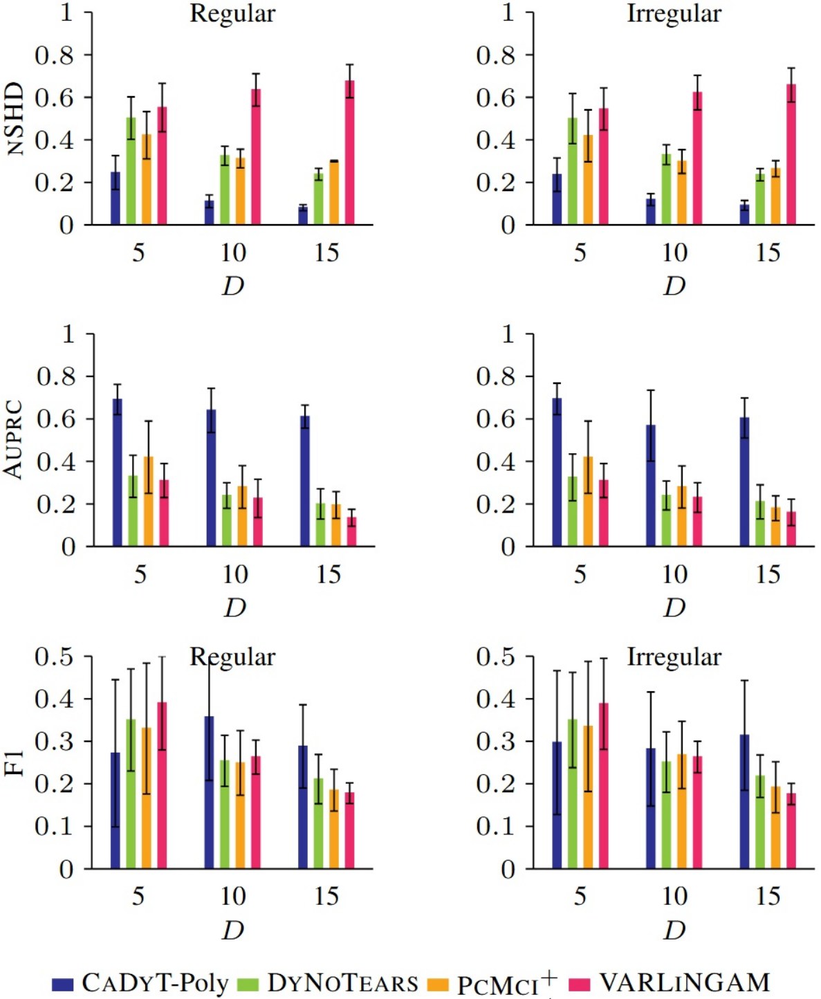
Figure B.1: [CaDyT with Polynomial Kernel] nSHD (top, lower is better), Auprc (middle, higher is better) F1 (bottom, higher is better) for random graphs of sizes for regularly sampled data (left) and irregularly sampled data (right).
图 B.1:[采用多项式核的 CaDyT] 随机图规模为 时,规则采样数据(左)与不规则采样数据(右)上的 nSHD(上,越低越好)、AUPRC(中,越高越好)和 F1(下,越高越好)。
| Method | nSHD | AUPRC |
|---|---|---|
| DyNoTears | 0.67 | 0.22 |
| 0.62 | 0.24 | |
| VARLiNGAM | 0.50 | 0.39 |
| CaDyT (ours) | 0.25 | 0.79 |
Table B.1: nSHD (Lower is better) and Auprc (Higher is better) for simulations on 2-mass spring system. The ground truth contains four variables and six edges. CaDyT ranks highest for both metrics.
| 方法 | nSHD | AUPRC |
|---|---|---|
| DyNoTears | 0.67 | 0.22 |
| 0.62 | 0.24 | |
| VARLiNGAM | 0.50 | 0.39 |
| CaDyT(本文) | 0.25 | 0.79 |
表 B.1:二质量弹簧系统仿真上的 nSHD(越低越好)与 AUPRC(越高越好)。真实结构含四个变量和六条边。CaDyT 在两项指标上都排在最前。
| Method | nSHD |
|---|---|
| DyNoTears | 0.25(0.00) |
| 0.04(0.04) | |
| VARLiNGAM | 0.02(0.04) |
| CaDyT (Poly) | 0.00(0.00) |
| CaDyT (RBF) | 0.00(0.00) |
Table B.2: nSHD (Lower is better) for simulations on the empty causal graph. The ground truth contains four variables and zero edges. Results are rounded to two decimal places. CaDyT ranks best, being capable of sensing the absence of causal relationships with both the RBF and the Polynomial Kernel, with every integrator (AB1, AB2, AB3).
| 方法 | nSHD |
|---|---|
| DyNoTears | 0.25(0.00) |
| 0.04(0.04) | |
| VARLiNGAM | 0.02(0.04) |
| CaDyT(多项式) | 0.00(0.00) |
| CaDyT(RBF) | 0.00(0.00) |
表 B.2:空因果图仿真上的 nSHD(越低越好)。真实结构含四个变量、零条边。结果四舍五入到两位小数。CaDyT 表现最好,无论使用 RBF 核还是多项式核,也无论使用哪种积分器(AB1、AB2、AB3),都能够察觉到不存在因果关系。
| Regular | Irregular | |||
|---|---|---|---|---|
| Method | nSHD | AUPRC | nSHD | AUPRC |
| DyNoTears | 0.694(0.074) | 0.168(0.023) | 0.650(0.094) | 0.184(0.033) |
| 0.450(0.039) | 0.132(0.023) | 0.462(0.462) | 0.139(0.030) | |
| VARLiNGAM | 0.668(0.072) | 0.174(0.009) | 0.612(0.064) | 0.181(0.013) |
| CaDyT (RBF) | 0.118(0.062) | 0.834(0.156) | 0.112(0.057) | 0.866(0.109) |
| CaDyT (Poly) | 0.106(0.083) | 0.883(0.199) | 0.087(0.073) | 0.925(0.191) |
Table B.3: nSHD (Lower is better) and Auprc (Higher is better) for simulations on the diamond causal graph. The ground truth contains four variables and four edges.
| 规则 | 不规则 | |||
|---|---|---|---|---|
| 方法 | nSHD | AUPRC | nSHD | AUPRC |
| DyNoTears | 0.694(0.074) | 0.168(0.023) | 0.650(0.094) | 0.184(0.033) |
| 0.450(0.039) | 0.132(0.023) | 0.462(0.462) | 0.139(0.030) | |
| VARLiNGAM | 0.668(0.072) | 0.174(0.009) | 0.612(0.064) | 0.181(0.013) |
| CaDyT(RBF) | 0.118(0.062) | 0.834(0.156) | 0.112(0.057) | 0.866(0.109) |
| CaDyT(多项式) | 0.106(0.083) | 0.883(0.199) | 0.087(0.073) | 0.925(0.191) |
表 B.3:钻石因果图仿真上的 nSHD(越低越好)与 AUPRC(越高越好)。真实结构含四个变量和四条边。
| Synthetic Double-Mass | Real Double-Linear | |||
|---|---|---|---|---|
| Method | nSHD | AUPRC | nSHD | AUPRC |
| DyNoTears | 0.675(0.109) | 0.224(0.045) | 0.625 | 0.590 |
| 0.618(0.095) | 0.244(0.039) | 0.500 | 0.306 | |
| VARLiNGAM | 0.500(0.029) | 0.386(0.000) | 0.500 | 0.441 |
| CaDyT (RBF) | 0.250(0.000) | 0.791(0.000) | 0.250 | 0.791 |
| CaDyT (Poly) | 0.250(0.000) | 0.791(0.000) | 0.375 | 0.687 |
Table B.4: nSHD (Lower is better) and Auprc (Higher is better) for simulations on the synthetic Double-Mass spring system and for the Real Double-Linear Spring system. The ground truth contains four variables and six edges. CaDyT ranks highest for both metrics when using the RBF kernel. An empty graph results on the real version when using a polynomial kernel.
| 仿真双质量 | 真实双线性 | |||
|---|---|---|---|---|
| 方法 | nSHD | AUPRC | nSHD | AUPRC |
| DyNoTears | 0.675(0.109) | 0.224(0.045) | 0.625 | 0.590 |
| 0.618(0.095) | 0.244(0.039) | 0.500 | 0.306 | |
| VARLiNGAM | 0.500(0.029) | 0.386(0.000) | 0.500 | 0.441 |
| CaDyT(RBF) | 0.250(0.000) | 0.791(0.000) | 0.250 | 0.791 |
| CaDyT(多项式) | 0.250(0.000) | 0.791(0.000) | 0.375 | 0.687 |
表 B.4:仿真双质量弹簧系统与真实双线性弹簧系统上的 nSHD(越低越好)与 AUPRC(越高越好)。真实结构含四个变量和六条边。使用 RBF 核时,CaDyT 在两项指标上都排在最前。使用多项式核时,在真实版本上会得到空图。
| Method | nSHD | AUPRC |
|---|---|---|
| DyNoTears | 0.314(0.163) | 0.336(0.187) |
| 0.337(0.046) | 0.219(0.054) | |
| VARLiNGAM | 0.507(0.099) | 0.299(0.066) |
| CaDyT (RBF) | 0.170(0.018) | 0.553(0.121) |
| CaDyT (Poly) | 0.166(0.021) | 0.592(0.130) |
Table B.5: nSHD (Lower is better) and Auprc (Higher is better) for the Rössler Oscillator. The ground truth contains 10 variables and Y edges. CaDyT ranks highest for both metrics.
| 方法 | nSHD | AUPRC |
|---|---|---|
| DyNoTears | 0.314(0.163) | 0.336(0.187) |
| 0.337(0.046) | 0.219(0.054) | |
| VARLiNGAM | 0.507(0.099) | 0.299(0.066) |
| CaDyT(RBF) | 0.170(0.018) | 0.553(0.121) |
| CaDyT(多项式) | 0.166(0.021) | 0.592(0.130) |
表 B.5:Rössler 振荡器上的 nSHD(越低越好)与 AUPRC(越高越好)。真实结构含 10 个变量和 Y 条边。CaDyT 在两项指标上都排在最前。
Appendix C Computational Analysis
附录 C 计算分析
Computation Complexity
The edge scoring phase performs a pairwise comparisons each involving GP-regression and priority queue updates whose complexity are resp. , resulting in complexity of . Both forward and backward search phases consider each present edge once and subsequently update at most edge scores, giving us a loose upper bound of , which is the overall complexity, by parallelizing this computation over edges, we can bring this down to in the best case.
计算复杂度
边打分阶段做 次成对比较,每次都涉及高斯过程回归和优先队列更新,复杂度分别为 与 ,因而总复杂度为 。前向与后向搜索阶段都会考虑每条已有边一次,并随后更新至多 条边的分数,从而给出一个较松的上界 ,这也是总体复杂度;若把该计算按边并行化,最好情况下可以降到 。
This is better than worst-case complexity of with Kernelized independence test, which is in in the worst-case. The complexity for VARLiNGAM is in because it assumes a parametric form of function between variables. We, nevertheless, see from our evaluation that while faster in practice, it achieves a sub-par performance. For DyNoTears there is no explicit Big‑O bound given in the original work but we note that evaluating the acyclicity constraint requires computing the matrix exponential of a adjacency matrix, which incurs a cost of at the very least.
这优于使用核化独立性检验的 的最坏情形复杂度,后者最坏为 。VARLiNGAM 的复杂度为 ,因为它假定变量之间的函数具有参数形式。不过,从我们的评估可以看到,尽管它在实践中更快,表现却明显较差。对 DyNoTears,原作没有给出显式的大 O 上界,但我们注意到,评估无环约束需要计算 邻接矩阵的矩阵指数,这至少会带来 的代价。
Runtime Analysis
In Table n:C.6, we provide runtime measurements on the Erdos-Renyi experiment. The main driver for its scalability is the chosen model class. Indeed, in our case the runtime is dominated by the time needed to train the GPs. Stronger scalability can be achieved by substituting GPs with a more lightweight model class.
运行时间分析
在表 C.6 中,我们给出 Erdős–Rényi 实验上的运行时间测量。其可扩展性的主要决定因素是所选模型类。在我们的情形中,运行时间由训练高斯过程所需的时间主导。若用更轻量的模型类替换高斯过程,可以获得更强的可扩展性。
| Runtime | |||
|---|---|---|---|
| Method | ER-5 | ER-10 | ER-15 |
| DyNoTears | 0.28(0.267) | 1.75(1.66) | 3.86(3.49) |
| 12.38(11.014) | 309.97(1513.29) | 84.25(40.05) | |
| VARLiNGAM | 0.12(0.031) | 0.54(0.17) | 1.48(0.50) |
| CaDyT (AB1/RBF) | 950.64(1834.42) | 2025.34(1389.26) | 4234.75(3125.90) |
| CaDyT (AB2/RBF) | 1292.11(1236.24) | 3653.92(2276.15) | 7448.01(3365.10) |
| CaDyT (AB3/RBF) | 2241.12(2437.72) | 6920.47(3559.90) | 9617.29(3735.26) |
| CaDyT (AB1/Poly) | 577.25(2082.06) | 484.63(67.17) | 940.66(149.99) |
| CaDyT (AB2/Poly) | 173.60(22.14) | 790.25(162.29) | 1564.18(238.23) |
| CaDyT (AB3/Poly) | 280.244(43.85) | 1178.49(199.63) | 2571.59(396.89) |
Table C.6: [Runtime for ER graphs of increasing size on regular timelines]: The runtime for CaDyT is highly dependent on the chosen model class. For our GP models, their training dominates the rest of the greedy-DAG search. Improved scalability can be achieved upon choosing a more lightweight model class.
| 运行时间 | |||
|---|---|---|---|
| 方法 | ER-5 | ER-10 | ER-15 |
| DyNoTears | 0.28(0.267) | 1.75(1.66) | 3.86(3.49) |
| 12.38(11.014) | 309.97(1513.29) | 84.25(40.05) | |
| VARLiNGAM | 0.12(0.031) | 0.54(0.17) | 1.48(0.50) |
| CaDyT(AB1/RBF) | 950.64(1834.42) | 2025.34(1389.26) | 4234.75(3125.90) |
| CaDyT(AB2/RBF) | 1292.11(1236.24) | 3653.92(2276.15) | 7448.01(3365.10) |
| CaDyT(AB3/RBF) | 2241.12(2437.72) | 6920.47(3559.90) | 9617.29(3735.26) |
| CaDyT(AB1/多项式) | 577.25(2082.06) | 484.63(67.17) | 940.66(149.99) |
| CaDyT(AB2/多项式) | 173.60(22.14) | 790.25(162.29) | 1564.18(238.23) |
| CaDyT(AB3/多项式) | 280.244(43.85) | 1178.49(199.63) | 2571.59(396.89) |
表 C.6:[规则时间轴上、规模递增的 ER 图的运行时间]:CaDyT 的运行时间高度依赖于所选模型类。对我们的高斯过程模型而言,其训练时间主导了其余的贪心 DAG 搜索。若选择更轻量的模型类,可扩展性还可以提高。
Appendix D Example of Scoring
附录 D 打分示例
Let us assume a simple scenario with variables and . Being a score-based method, CaDyT will search for the combination of parents minimizing our designed score. Therefore, CaDyT needs to decide between the sets , , or , and will do so by searching (greedily) the one with with lowest score. In this section, we present an operative and step-by-step example on how to score the GP when the candidate parents are and .
假定一个简单情形,变量为 和 。作为基于分数的方法,CaDyT 会搜索使所设计分数最小的父节点组合。因此,CaDyT 需要在集合 、 或 之间做选择,并将(贪心地)搜索分数最低的那一个。本节给出一个可操作的逐步示例,说明当候选父节点为 和 时,如何对高斯过程打分。
Scoring :
对 打分:
We want to show how our score will be computed when the parent set of is . We will go through how each term of the score is computed
我们要说明,当 的父节点集合为 时,分数如何计算。我们将逐项说明分数中每一项的计算方式。
First, we fit a local model , and later we score that model. As a model class, we use the GPs in (Ensinger et al. 2024) to learn the continuous-dynamics associated to as a function of and , which is . After training the GP, the scoring procedure can start. What is necessary is to encode the model’s parameters (function cost), its causal parents (structure cost), and the data-given-model cost. Function cost and structure cost are the two parts of Eq.13, which we recall below
首先,我们拟合局部模型 ,随后对该模型打分。作为模型类,我们使用 (Ensinger et al. 2024) 中的高斯过程,把与 相关的连续动力学学习成 和 的函数,即 。高斯过程训练完成后,即可开始打分。需要编码的是模型参数(函数成本)、其因果父节点(结构成本),以及给定模型后的数据成本。函数成本与结构成本是式 (13) 的两个部分,我们在下面重述
Computing the Function Cost
The function cost is computed by encoding the length scale , variance , and eigenvalues in using . Each one of those is encoded by using defined in Eq.16. In practice, the function cost is obtained by summing all the entries of the encoded length-scale vector, the encoded noise variance, and the encoded eigenvalues in .
计算函数成本
函数成本通过对长度尺度 、方差 以及 中的特征值用 编码来计算。每一项都用式 (16) 定义的 编码。实践中,函数成本 由编码后的长度尺度向量、编码后的噪声方差,以及 中编码后的特征值各分量求和得到。
Computing the Structure Cost
The structure cost encodes the chosen causal parents, and it is composed by two terms. The first one is just an optimal encoding for integers (Rissanen 1983) for the number of causal parents, that in our case are and , implying that . Similarly, we also have another term . Therefore, the structure cost is .
计算结构成本
结构成本对所选因果父节点编码,由两项组成。第一项只是对整数的最优编码(Rissanen 1983),用来编码因果父节点的个数;在我们的情形中是 和 ,因此 。类似地,还有另一项 。因此,结构成本为 。
Computing Data-given-Model Cost
We use the GP for to predict the trajectory over the timeline . We then need to compute an empirical estimate of the residual noise variance:
计算给定模型后的数据成本
我们用 的高斯过程,在时间轴 上预测轨迹 。然后需要计算残差噪声方差的经验估计:
where refers to the ground truth trajectory for . The resulting quantity is then used to encode using Eq.(17) and resulting in .
其中 表示 的真实轨迹。得到的量随后用式 (17) 对 编码,从而得到 。
Summing All the Terms
Finally, all the above-mentioned terms have to be summed together, yielding
把各项相加
最后,把上述各项加在一起,得到
Scoring with no Parents
没有父节点时的打分
During the initial edge scoring phase (See algorithm 2), scores need to be computed also for the case in which there are no parents. In this case, we just encode the mean value of over which we indicate as .
在最初的边打分阶段(见算法 2),还需要对没有父节点的情形计算分数。这时,我们只编码 关于 的均值,记为 。
Function Cost
This time there are no parents or self-loops. Therefore, instead of scoring a trained model, we just encode the mean value of , i.e. we use Eq.16 to encode .
函数成本
这时没有父节点,也没有自环。因此,我们不对训练好的模型打分,而只编码 的均值,即用式 (16) 编码 。
Computing Data-given-Model cost
Our estimate of the residual noise variance is consequently computed between and its mean. Therefore, we have
计算给定模型后的数据成本
我们对残差噪声方差的估计,因而在 与其均值之间计算。于是有
Appendix E Algorithms Pseudo-code
附录 E 算法伪代码
1:
2:
3:
4:
Algorithm 1 CaDyT for timeseries causal discovery
1:
2:
3:
4:
算法 1 面向时间序列因果发现的 CaDyT
For ease of reading, we again describe our score-based method Causal Discovery for Dynamic Timeseries (CaDyT ) for discovering causal graphs of multivariate continuous-valued dynamical systems. We incorporate our proposed score into a common three-step search procedure (Mian, Marx, and Vreeken 2021; Mameche, Kaltenpoth, and Vreeken 2023) namely, edge scoring, forward and backward search, as shown in Alg. 1. This is the next best alternative to exhaustive search for our case. The well known Greedy Equivalence Search (Chickering 2002) is not built for timeseries and methods for topological search (Wang et al. 2017; Xu, Mameche, and Vreeken 2025) do not directly apply to cyclic systems. We provide our code in the supplementary material.
为便于阅读,我们再次描述基于分数的方法——面向动态时间序列的因果发现(Causal Discovery for Dynamic Timeseries,CaDyT),用于发现多元连续值动力系统的因果图。我们把提出的分数纳入常见的三步搜索流程(Mian, Marx, and Vreeken 2021;Mameche, Kaltenpoth, and Vreeken 2023),即边打分、前向搜索和后向搜索,如算法 1 所示。就我们的情形而言,这是穷尽搜索之外的次优但可实用的替代。众所周知的贪心等价搜索(Chickering 2002)并非为时间序列而建,面向拓扑搜索的方法(Wang et al. 2017;Xu, Mameche, and Vreeken 2025)也不能直接用于有环系统。代码放在补充材料中。
We start with the edge-ranking phase that computes the gain for all pairwise causal connections. The gain , between each pair and , is given by
我们从边排序阶段开始,计算所有成对因果连接的增益。每对 与 之间的增益 由下式给出
where implies model with edge included. Intuitively, the higher the , the more confident we are that this is the correct causal edge. The edge scoring phase returns a priority queue of tuples ordered by decreasing gain.
其中 表示在模型 中加入边 后的模型。直观上, 越高,我们越有把握认为这是正确的因果边。边打分阶段返回按增益降序排列的元组优先队列 。
The forward search iteratively adds the highest-scoring edge from the priority queue. After adding an edge , all incoming edges to are re-evaluated using Eq. (18) and updated in the queue. Before inclusion, each edge is tested for statistical significance using the no-hypercompression inequality (Grünwald 2007). The search terminates when no further additions improve the score. The subsequent backward phase prunes redundant edges by removing any whose deletion increases , continuing until no such edges remain. We then return the final graph.
前向搜索迭代地从优先队列中加入得分最高的边。加入边 之后,所有指向 的入边都按式 (18) 重新评估,并在队列中更新。在纳入之前,每条边都用无超压缩不等式(Grünwald 2007)做统计显著性检验。当再加入边无法改进分数时,搜索终止。随后的后向阶段会剪掉冗余边:删去任何一条会使 增大的边,直到不再存在这样的边。然后我们返回最终的图。
CaDyT has overall computational complexity of where derives from our choice of non-parametric regression functions (GPs) for . In appendix C, we give a detailed derivation on the computational complexity and show how it is at least on-par with existing methods. CaDyT , moreover, can be inherently parallelized, and we implement it as such, resulting in a fast runtime.
CaDyT 的总体计算复杂度为 ,其中 来自我们为 选择的非参数回归函数(高斯过程)。附录 C 给出计算复杂度的详细推导,并说明它至少不弱于现有方法。此外,CaDyT 本质上可以并行,我们也按并行方式实现,因而运行较快。
1: while do
2:
3: end while
4:
Algorithm 2 EdgeScoring
1: while do
2:
3: end while
4:
算法 2 边打分(EdgeScoring)
1:
2:
3: for each do
4: if then
5:
6: end if
7: end for
8:
9: while do
10:
11:
12: for each do
13: if then
14:
15:
16:
17:
18: if then
19:
20:
21: end if
22: end if
23: end for
24: if then
25:
26: else
27:
28: end if
29: end while
30:
Algorithm 3 ForwardSearch
1:
2:
3: for each do
4: if then
5:
6: end if
7: end for
8:
9: while do
10:
11:
12: for each do
13: if then
14:
15:
16:
17:
18: if then
19:
20:
21: end if
22: end if
23: end for
24: if then
25:
26: else
27:
28: end if
29: end while
30:
算法 3 前向搜索(ForwardSearch)
1:
2: while do
3:
4:
5:
6: for each do
7:
8:
9:
10:
11: if then
12:
13:
14: end if
15: end for
16: if then
17:
18: else
19:
20: end if
21: end while
22:
Algorithm 4 BackwardSearch
1:
2: while do
3:
4:
5:
6: for each do
7:
8:
9:
10:
11: if then
12:
13:
14: end if
15: end for
16: if then
17:
18: else
19:
20: end if
21: end while
22:
算法 4 后向搜索(BackwardSearch)