Bootstrap Your Own Latent: A New Approach to Self-Supervised Learning
Bootstrap Your Own Latent A New Approach to Self-Supervised Learning
Bootstrap Your Own Latent:一种新的自监督学习方法
Jean-Bastien Grill Florian Strub 1 1 footnotemark: 1 Florent Altché 1 1 footnotemark: 1 Corentin Tallec 1 1 footnotemark: 1 Pierre H. Richemond 1 1 footnotemark: 1 † † thanks: Equal contribution; the order of first authors was randomly selected. Affiliation: DeepMind Affiliation: Imperial College Elena Buchatskaya Carl Doersch Bernardo Avila Pires Zhaohan Daniel Guo Affiliation: DeepMind Mohammad Gheshlaghi Azar Bilal Piot Koray Kavukcuoglu Rémi Munos Michal Valko Email: [jbgrill,fstrub,altche,corentint,richemond]@google.com Affiliation: DeepMind
Abstract
摘要
We introduce Bootstrap Your Own Latent (BYOL), a new approach to self-supervised image representation learning. BYOL relies on two neural networks, referred to as online and target networks, that interact and learn from each other. From an augmented view of an image, we train the online network to predict the target network representation of the same image under a different augmented view. At the same time, we update the target network with a slow-moving average of the online network. While state-of-the art methods rely on negative pairs, BYOL achieves a new state of the art without them. BYOL reaches top-1 classification accuracy on ImageNet using a linear evaluation with a ResNet-50 architecture and with a larger ResNet. We show that BYOL performs on par or better than the current state of the art on both transfer and semi-supervised benchmarks. Our implementation and pretrained models are given on GitHub.[^3]
我们提出 Bootstrap Your Own Latent(BYOL),一种新的自监督图像表征学习方法。BYOL 依赖两个神经网络——分别称为在线网络与目标网络——彼此交互、互相学习。给定一幅图像的增强视图,我们训练在线网络去预测同一图像在另一增强视图下由目标网络给出的表征;与此同时,用在线网络参数的慢速滑动平均更新目标网络。当前最先进方法依赖负样本对,而 BYOL 不使用负样本 即达到新的最优水平。在 ImageNet 上,用线性评估协议,ResNet-50 达到 top-1 分类精度,更大 ResNet 达到 。我们表明 BYOL 在迁移与半监督基准上与当前最优持平或更优。实现与预训练模型见 GitHub。
1 Introduction
1 引言
[1, 2, 3, 4, 5, 6, 7]
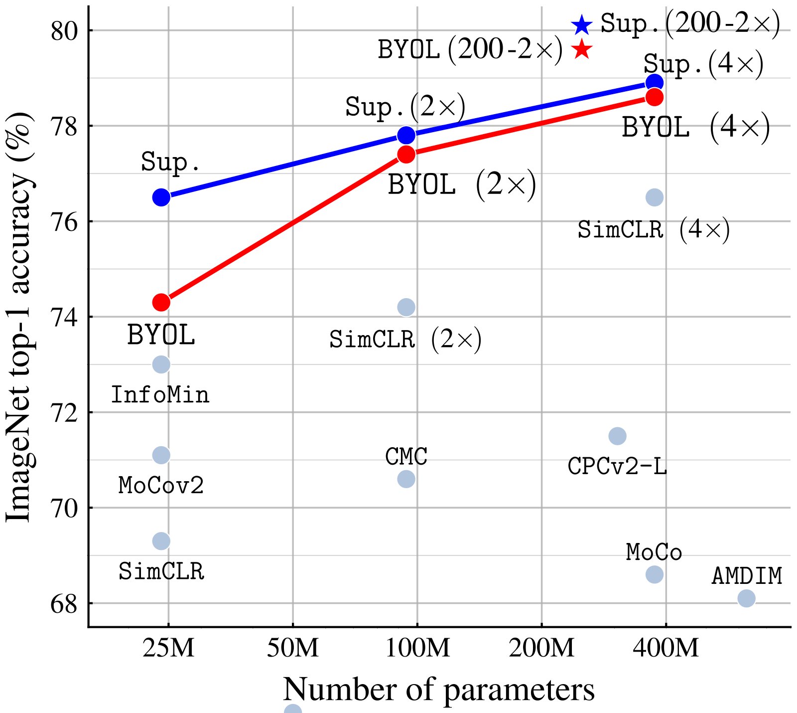
Figure 1: Performance of BYOL on ImageNet (linear evaluation) using ResNet-50 and our best architecture ResNet-200 (), compared to other unsupervised and supervised (Sup.) baselines [8].
图 1:BYOL 在 ImageNet(线性评估)上使用 ResNet-50 以及我们最好架构 ResNet-200()的表现,并与其他无监督及监督(Sup.)基线对比 [8]。
Learning good image representations is a key challenge in computer vision [1, 2, 3] as it allows for efficient training on downstream tasks [4, 5, 6, 7]. Many different training approaches have been proposed to learn such representations, usually relying on visual pretext tasks. Among them, state-of-the-art contrastive methods [8, 9, 10, 11, 12] are trained by reducing the distance between representations of different augmented views of the same image (‘positive pairs’), and increasing the distance between representations of augmented views from different images (‘negative pairs’). These methods need careful treatment of negative pairs [13] by either relying on large batch sizes [8, 12], memory banks [9] or customized mining strategies [14, 15] to retrieve the negative pairs. In addition, their performance critically depends on the choice of image augmentations [8, 12].
学习良好的图像表征是计算机视觉的关键挑战 [1, 2, 3],因为它能让下游任务更高效地训练 [4, 5, 6, 7]。人们提出了许多训练此类表征的方法,通常依赖视觉代理任务。其中,当前最优的对比方法 [8, 9, 10, 11, 12] 通过缩小同一图像不同增强视图表征之间的距离(「正样本对」),并增大不同图像增强视图表征之间的距离(「负样本对」)来训练。这些方法需要谨慎处理负样本对 [13],要么依赖大批次 [8, 12]、记忆库 [9],要么定制挖掘策略 [14, 15] 来获取负样本。此外,其表现严重依赖图像增强的选择 [8, 12]。
In this paper, we introduce Bootstrap Your Own Latent (BYOL), a new algorithm for self-supervised learning of image representations. BYOL achieves higher performance than state-of-the-art contrastive methods without using negative pairs. It iteratively bootstraps[^4] the outputs of a network to serve as targets for an enhanced representation. Moreover, BYOL is more robust to the choice of image augmentations than contrastive methods; we suspect that not relying on negative pairs is one of the leading reasons for its improved robustness. While previous methods based on bootstrapping have used pseudo-labels [16], cluster indices [17] or a handful of labels [18, 19, 20], we propose to directly bootstrap the representations. In particular, BYOL uses two neural networks, referred to as online and target networks, that interact and learn from each other. Starting from an augmented view of an image, BYOL trains its online network to predict the target network’s representation of another augmented view of the same image. While this objective admits collapsed solutions, e.g., outputting the same vector for all images, we empirically show that BYOL does not converge to such solutions. We hypothesize (see Section 3.2) that the combination of (i) the addition of a predictor to the online network and (ii) the use of a slow-moving average of the online parameters as the target network encourages encoding more and more information within the online projection and avoids collapsed solutions.
本文提出 Bootstrap Your Own Latent(BYOL),一种新的图像表征自监督学习算法。BYOL 在不使用负样本对的情况下,取得高于当前最优对比方法的表现。它迭代地自举网络输出,作为增强表征的目标。此外,BYOL 对图像增强选择比对比方法更稳健;我们怀疑不依赖负样本对是稳健性提升的主因之一。先前基于自举的方法使用伪标签 [16]、聚类索引 [17] 或少量标签 [18, 19, 20],我们则提出直接自举表征。具体地,BYOL 使用在线与目标两个神经网络彼此交互学习。从一幅图像的增强视图出发,BYOL 训练在线网络去预测目标网络对同一图像另一增强视图的表征。该目标虽允许崩塌解(例如对所有图像输出同一向量),但我们经验上表明 BYOL 不会收敛到这类解。我们猜想(见第 3.2 节):(i) 在在线网络上增加预测器,以及 (ii) 用在线参数的慢速滑动平均作为目标网络,二者结合会鼓励在线投影编码越来越多的信息,并避免崩塌解。
We evaluate the representation learned by BYOL on ImageNet [21] and other vision benchmarks using ResNet architectures [22]. Under the linear evaluation protocol on ImageNet, consisting in training a linear classifier on top of the frozen representation, BYOL reaches top-1 accuracy with a standard ResNet- and top-1 accuracy with a larger ResNet (Figure 1). In the semi-supervised and transfer settings on ImageNet, we obtain results on par or superior to the current state of the art. Our contributions are: (i) We introduce BYOL, a self-supervised representation learning method (Section 3) which achieves state-of-the-art results under the linear evaluation protocol on ImageNet without using negative pairs. (ii) We show that our learned representation outperforms the state of the art on semi-supervised and transfer benchmarks (Section 4). (iii) We show that BYOL is more resilient to changes in the batch size and in the set of image augmentations compared to its contrastive counterparts (Section 5). In particular, BYOL suffers a much smaller performance drop than SimCLR, a strong contrastive baseline, when only using random crops as image augmentations.
我们在 ImageNet [21] 及其他视觉基准上,用 ResNet 架构 [22] 评估 BYOL 学到的表征。在 ImageNet 线性评估协议下——即在冻结表征上训练线性分类器——标准 ResNet-50 达到 top-1 精度,更大 ResNet 达到 top-1 精度(图 1)。在 ImageNet 半监督与迁移设置中,结果与当前最优持平或更优。我们的贡献是:(i) 提出 BYOL(第 3 节),一种不使用负样本对、在 ImageNet 线性评估协议下达到最优的自监督表征学习方法;(ii) 表明所学表征在半监督与迁移基准上优于当前最优(第 4 节);(iii) 表明 BYOL 相对对比方法对批次大小与图像增强集合的变化更有韧性(第 5 节)。特别是,当只使用随机裁剪作为图像增强时,BYOL 的性能下降远小于强对比基线 SimCLR。
2 Related work
2 相关工作
Most unsupervised methods for representation learning can be categorized as either generative or discriminative [23, 8]. Generative approaches to representation learning build a distribution over data and latent embedding and use the learned embeddings as image representations. Many of these approaches rely either on auto-encoding of images [24, 25, 26] or on adversarial learning [27], jointly modelling data and representation [28, 29, 30, 31]. Generative methods typically operate directly in pixel space. This however is computationally expensive, and the high level of detail required for image generation may not be necessary for representation learning.
多数无监督表征学习方法可归为生成式或判别式 [23, 8]。生成式方法在数据与隐嵌入上建立分布,并把学到的嵌入当作图像表征。其中许多依赖图像自编码 [24, 25, 26] 或对抗学习 [27],联合建模数据与表征 [28, 29, 30, 31]。生成式方法通常直接在像素空间操作,计算昂贵,且图像生成所需的高细节对表征学习未必必要。
Among discriminative methods, contrastive methods [9, 10, 32, 33, 34, 11, 35, 36] currently achieve state-of-the-art performance in self-supervised learning [37, 8, 38, 12]. Contrastive approaches avoid a costly generation step in pixel space by bringing representation of different views of the same image closer (‘positive pairs’), and spreading representations of views from different images (‘negative pairs’) apart [39, 40]. Contrastive methods often require comparing each example with many other examples to work well [9, 8] prompting the question of whether using negative pairs is necessary.
在判别式方法中,对比方法 [9, 10, 32, 33, 34, 11, 35, 36] 目前在自监督学习中表现最优 [37, 8, 38, 12]。对比方法通过拉近同一图像不同视图的表征(「正样本对」)、推远不同图像视图的表征(「负样本对」)[39, 40],避免在像素空间做昂贵生成。对比方法往往需要把每个样本与许多其他样本比较才能工作得好 [9, 8],于是引出负样本对是否必要的问题。
DeepCluster [17] partially answers this question. It uses bootstrapping on previous versions of its representation to produce targets for the next representation; it clusters data points using the prior representation, and uses the cluster index of each sample as a classification target for the new representation. While avoiding the use of negative pairs, this requires a costly clustering phase and specific precautions to avoid collapsing to trivial solutions.
DeepCluster [17] 部分回答了该问题。它对自己先前版本的表征做自举,为下一表征产生目标:用先前表征对数据点聚类,并把每个样本的聚类索引当作新表征的分类目标。虽然避免了负样本对,但这需要昂贵的聚类阶段,并需采取特定防范以避免崩塌到平凡解。
Some self-supervised methods are not contrastive but rely on using auxiliary handcrafted prediction tasks to learn their representation. In particular, relative patch prediction [23, 40], colorizing gray-scale images [41, 42], image inpainting [43], image jigsaw puzzle [44], image super-resolution [45], and geometric transformations [46, 47] have been shown to be useful. Yet, even with suitable architectures [48], these methods are being outperformed by contrastive methods [37, 8, 12].
一些自监督方法不是对比式的,而是依赖手工设计的辅助预测任务来学习表征。相对图块预测 [23, 40]、灰度图上色 [41, 42]、图像修复 [43]、拼图 [44]、超分辨率 [45] 以及几何变换 [46, 47] 都被证明有用。然而即便有合适架构 [48],这些方法也正被对比方法超越 [37, 8, 12]。
Our approach has some similarities with Predictions of Bootstrapped Latents (PBL, [49]), a self-supervised representation learning technique for reinforcement learning (RL). PBL jointly trains the agent’s history representation and an encoding of future observations. The observation encoding is used as a target to train the agent’s representation, and the agent’s representation as a target to train the observation encoding. Unlike PBL, BYOL uses a slow-moving average of its representation to provide its targets, and does not require a second network.
我们的方法与强化学习中的自监督表征学习技术 Predictions of Bootstrapped Latents(PBL,[49])有一些相似。PBL 联合训练智能体历史表征与未来观测编码。观测编码用作训练智能体表征的目标,智能体表征又用作训练观测编码的目标。与 PBL 不同,BYOL 用自身表征的慢速滑动平均提供目标,且不需要第二个网络。
The idea of using a slow-moving average target network to produce stable targets for the online network was inspired by deep RL [50, 51, 52, 53]. Target networks stabilize the bootstrapping updates provided by the Bellman equation, making them appealing to stabilize the bootstrap mechanism in BYOL. While most RL methods use fixed target networks, BYOL uses a weighted moving average of previous networks (as in [54]) in order to provide smoother changes in the target representation.
用慢速滑动平均目标网络为在线网络产生稳定目标的想法,受深度强化学习启发 [50, 51, 52, 53]。目标网络稳定贝尔曼方程提供的自举更新,因而也适合稳定 BYOL 中的自举机制。多数 RL 方法使用固定目标网络,而 BYOL 使用先前网络的加权滑动平均(如 [54]),以使目标表征变化更平滑。
In the semi-supervised setting [55, 56], an unsupervised loss is combined with a classification loss over a handful of labels to ground the training [19, 20, 57, 58, 59, 60, 61, 62]. Among these methods, mean teacher (MT) [20] also uses a slow-moving average network, called teacher, to produce targets for an online network, called student. An consistency loss between the softmax predictions of the teacher and the student is added to the classification loss. While [20] demonstrates the effectiveness of MT in the semi-supervised learning case, in Section 5 we show that a similar approach collapses when removing the classification loss. In contrast, BYOL introduces an additional predictor on top of the online network, which prevents collapse.
在半监督设置中 [55, 56],无监督损失与少量标签上的分类损失结合,以锚定训练 [19, 20, 57, 58, 59, 60, 61, 62]。其中 mean teacher(MT)[20] 也使用慢速滑动平均网络(称为教师)为在线网络(称为学生)产生目标。教师与学生 softmax 预测之间的 一致性损失被加到分类损失上。[20] 证明了 MT 在半监督学习中的有效性,但在第 5 节我们表明:去掉分类损失后,类似做法会崩塌。相比之下,BYOL 在在线网络之上引入额外预测器,从而防止崩塌。
Finally, in self-supervised learning, MoCo [9] uses a slow-moving average network (momentum encoder) to maintain consistent representations of negative pairs drawn from a memory bank. Instead, BYOL uses a moving average network to produce prediction targets as a means of stabilizing the bootstrap step. We show in Section 5 that this mere stabilizing effect can also improve existing contrastive methods.
最后,在自监督学习中,MoCo [9] 使用慢速滑动平均网络(动量编码器)来维护从记忆库抽取的负样本对的一致表征。BYOL 则用滑动平均网络产生预测目标,作为稳定自举步骤的手段。我们在第 5 节表明,这一单纯的稳定效果也能改进现有对比方法。
3 Method
3 方法
We start by motivating our method before explaining its details in Section 3.1. Many successful self-supervised learning approaches build upon the cross-view prediction framework introduced in [63]. Typically, these approaches learn representations by predicting different views (e.g., different random crops) of the same image from one another. Many such approaches cast the prediction problem directly in representation space: the representation of an augmented view of an image should be predictive of the representation of another augmented view of the same image. However, predicting directly in representation space can lead to collapsed representations: for instance, a representation that is constant across views is always fully predictive of itself. Contrastive methods circumvent this problem by reformulating the prediction problem into one of discrimination: from the representation of an augmented view, they learn to discriminate between the representation of another augmented view of the same image, and the representations of augmented views of different images. In the vast majority of cases, this prevents the training from finding collapsed representations. Yet, this discriminative approach typically requires comparing each representation of an augmented view with many negative examples, to find ones sufficiently close to make the discrimination task challenging. In this work, we thus tasked ourselves to find out whether these negative examples are indispensable to prevent collapsing while preserving high performance.
我们先说明动机,再在第 3.1 节给出细节。许多成功的自监督学习方法建立在 [63] 提出的跨视图预测框架之上。这些方法通常通过从一个视图预测同一图像的另一视图(例如不同随机裁剪)来学习表征。许多方法把预测问题直接放在表征空间:一幅图像增强视图的表征应能预测同一图像另一增强视图的表征。然而直接在表征空间预测可能导致崩塌表征:例如跨视图恒定的表征总是能完全预测自身。对比方法把预测改写成判别:从一幅增强视图的表征出发,学会把同一图像另一增强视图的表征,与不同图像增强视图的表征区分开。绝大多数情况下,这能防止训练找到崩塌表征。但这种判别做法通常需要把每个增强视图的表征与大量负例比较,才能找到足够接近、使判别任务具有挑战性的样本。因此,本工作的任务是弄清:负例对于防止崩塌同时保持高性能是否必不可少。
To prevent collapse, a straightforward solution is to use a fixed randomly initialized network to produce the targets for our predictions. While avoiding collapse, it empirically does not result in very good representations. Nonetheless, it is interesting to note that the representation obtained using this procedure can already be much better than the initial fixed representation. In our ablation study (Section 5), we apply this procedure by predicting a fixed randomly initialized network and achieve top-1 accuracy (Table 5(a)) on the linear evaluation protocol on ImageNet, whereas the randomly initialized network only achieves by itself. This experimental finding is the core motivation for BYOL: from a given representation, referred to as target, we can train a new, potentially enhanced representation, referred to as online, by predicting the target representation. From there, we can expect to build a sequence of representations of increasing quality by iterating this procedure, using subsequent online networks as new target networks for further training. In practice, BYOL generalizes this bootstrapping procedure by iteratively refining its representation, but using a slowly moving exponential average of the online network as the target network instead of fixed checkpoints.
为防止崩塌,一个直接办法是用固定的随机初始化网络产生预测目标。虽能避免崩塌,但经验上得不到很好的表征。有趣的是,用该流程得到的表征已经可以远好于初始固定表征。在消融(第 5 节)中,我们预测一个固定随机初始化网络,在 ImageNet 线性评估上达到 top-1 精度(表 5(a)),而随机初始化网络本身只有 。这一实验发现是 BYOL 的核心动机:从给定表征(称为目标)出发,可通过预测目标表征来训练新的、可能更强的表征(称为在线)。由此可期望通过迭代该流程、把后续在线网络当作新的目标网络继续训练,构建质量递增的表征序列。实践中,BYOL 推广这一自举流程,迭代 refinement 其表征,但用在线网络的慢速指数滑动平均作为目标网络,而不是固定检查点。
3.1 Description of BYOL
3.1 BYOL 的描述
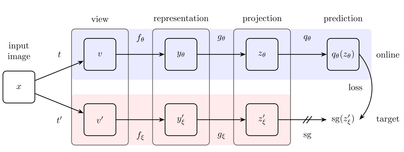
Figure 2: BYOL’s architecture. BYOL minimizes a similarity loss between and , where are the trained weights, are an exponential moving average of and means stop-gradient. At the end of training, everything but is discarded, and is used as the image representation.
图 2:BYOL 的架构。BYOL 最小化 与 之间的相似性损失,其中 是训练权重, 是 的指数滑动平均, 表示停止梯度。训练结束时,除 外全部丢弃,并用 作为图像表征。
BYOL’s goal is to learn a representation which can then be used for downstream tasks. As described previously, BYOL uses two neural networks to learn: the online and target networks. The online network is defined by a set of weights and is comprised of three stages: an encoder , a projector and a predictor , as shown in Figure 2 and Figure 8. The target network has the same architecture as the online network, but uses a different set of weights . The target network provides the regression targets to train the online network, and its parameters are an exponential moving average of the online parameters [54]. More precisely, given a target decay rate , after each training step we perform the following update,
BYOL 的目标是学习可用于下游任务的表征 。如前所述,BYOL 用两个神经网络学习:在线网络与目标网络。在线网络由权重 定义,包含三个阶段:编码器 、投影器 与预测器 ,如图 2 与图 8 所示。目标网络架构与在线网络相同,但使用不同权重集 。目标网络为训练在线网络提供回归目标,其参数 是在线参数 的指数滑动平均 [54]。更精确地,给定目标衰减率 ,每一步训练后执行如下更新,
Given a set of images , an image sampled uniformly from , and two distributions of image augmentations and , BYOL produces two augmented views v\mathrel{\hbox{\hskip 3.8889pt\hskip-3.8889pt\hbox{=}\hskip-3.8889pt\hskip-2.7431pt\raisebox{4.66875pt}{\hbox{\scriptscriptstyle\Delta}}\hskip-2.7431pt\hskip 3.8889pt}}t(x) and v^{\prime}\mathrel{\hbox{\hskip 3.8889pt\hskip-3.8889pt\hbox{=}\hskip-3.8889pt\hskip-2.7431pt\raisebox{4.66875pt}{\hbox{\scriptscriptstyle\Delta}}\hskip-2.7431pt\hskip 3.8889pt}}t^{\prime}(x) from by applying respectively image augmentations and . From the first augmented view , the online network outputs a representation y_{\theta}\mathrel{\hbox{\hskip 3.8889pt\hskip-3.8889pt\hbox{=}\hskip-3.8889pt\hskip-2.7431pt\raisebox{4.66875pt}{\hbox{\scriptscriptstyle\Delta}}\hskip-2.7431pt\hskip 3.8889pt}}f_{\theta}(v) and a projection z_{\theta}\mathrel{\hbox{\hskip 3.8889pt\hskip-3.8889pt\hbox{=}\hskip-3.8889pt\hskip-2.7431pt\raisebox{4.66875pt}{\hbox{\scriptscriptstyle\Delta}}\hskip-2.7431pt\hskip 3.8889pt}}g_{\theta}(y). The target network outputs y^{\prime}_{\xi}\mathrel{\hbox{\hskip 3.8889pt\hskip-3.8889pt\hbox{=}\hskip-3.8889pt\hskip-2.7431pt\raisebox{4.66875pt}{\hbox{\scriptscriptstyle\Delta}}\hskip-2.7431pt\hskip 3.8889pt}}f_{\xi}(v^{\prime}) and the target projection z^{\prime}_{\xi}\mathrel{\hbox{\hskip 3.8889pt\hskip-3.8889pt\hbox{=}\hskip-3.8889pt\hskip-2.7431pt\raisebox{4.66875pt}{\hbox{\scriptscriptstyle\Delta}}\hskip-2.7431pt\hskip 3.8889pt}}g_{\xi}(y^{\prime}) from the second augmented view . We then output a prediction of and -normalize both and to \overline{q_{\theta}}(z_{\theta})\mathrel{\hbox{\hskip 3.8889pt\hskip-3.8889pt\hbox{=}\hskip-3.8889pt\hskip-2.7431pt\raisebox{4.66875pt}{\hbox{\scriptscriptstyle\Delta}}\hskip-2.7431pt\hskip 3.8889pt}}q_{\theta}(z_{\theta})/\mathopen{}\mathclose{{\left\|q_{\theta}(z_{\theta})}}\right\|_{2} and \overline{z}^{\prime}_{\xi}\mathrel{\hbox{\hskip 3.8889pt\hskip-3.8889pt\hbox{=}\hskip-3.8889pt\hskip-2.7431pt\raisebox{4.66875pt}{\hbox{\scriptscriptstyle\Delta}}\hskip-2.7431pt\hskip 3.8889pt}}z^{\prime}_{\xi}/\|z^{\prime}_{\xi}\|_{2}. Note that this predictor is only applied to the online branch, making the architecture asymmetric between the online and target pipeline. Finally we define the following mean squared error between the normalized predictions and target projections,[^5]
给定图像集 ,从 均匀采样图像 ,以及两组图像增强分布 与 ,BYOL 分别施加增强 与 ,从 产生两个增强视图 与 。从第一个增强视图 ,在线网络输出表征 与投影 。目标网络从第二个增强视图 输出 与目标投影 。然后我们输出对 的预测 ,并把 与 都做 归一化。注意预测器只加在在线分支,使在线与目标流水线不对称。最后,我们定义归一化预测与目标投影之间的均方误差,
\mathcal{L}_{{\theta},\xi}\mathrel{\hbox{\hskip 3.8889pt\hskip-3.8889pt\hbox{$=$}\hskip-3.8889pt\hskip-2.7431pt\raisebox{4.66875pt}{\hbox{$\scriptscriptstyle\Delta$}}\hskip-2.7431pt\hskip 3.8889pt}}\mathopen{}\mathclose{{\left\|\overline{q_{\theta}}(z_{\theta})-\overline{z}^{\prime}_{\xi}}}\right\|_{2}^{2}=2-2\cdot\frac{\langle q_{\theta}(z_{\theta}),z^{\prime}_{\xi}\rangle}{\big\|q_{\theta}(z_{\theta})\big\|_{2}\cdot\big\|z^{\prime}_{\xi}\big\|_{2}}\cdot \tag{2}
We symmetrize the loss in Equation 2 by separately feeding to the online network and to the target network to compute . At each training step, we perform a stochastic optimization step to minimize with respect to only, but not , as depicted by the stop-gradient in Figure 2. BYOL’s dynamics are summarized as
我们通过分别把 送入在线网络、把 送入目标网络来计算 ,从而对称化方程 2 中的损失 。每一步训练中,我们对 (而不是 )做随机优化步,以最小化 ,如图 2 中的停止梯度所示。BYOL 的动态可概括为
\displaystyle{\theta}\leftarrow\mathrm{optimizer}\mathopen{}\mathclose{{\left({\theta},\nabla_{\theta}\mathcal{L}^{\texttt{BYOL}}_{{\theta},\xi},\eta}}\right), \\ \displaystyle\xi\leftarrow\tau\xi+(1-\tau){\theta}, \tag{3}
where is an optimizer and is a learning rate.
其中 是优化器, 是学习率。
At the end of training, we only keep the encoder ; as in [9]. When comparing to other methods, we consider the number of inference-time weights only in the final representation . The full training procedure is summarized in Appendix A, and python pseudo-code based on the libraries JAX [64] and Haiku [65] is provided in in Appendix J.
训练结束时,我们只保留编码器 ;与 [9] 相同。与其他方法比较时,我们只计最终表征 中推理时权重的数量。完整训练流程见附录 A;基于 JAX [64] 与 Haiku [65] 的 python 伪代码见附录 J。
3.2 Intuitions on BYOL’s behavior
3.2 关于 BYOL 行为的直觉
As BYOL does not use an explicit term to prevent collapse (such as negative examples [10]) while minimizing with respect to , it may seem that BYOL should converge to a minimum of this loss with respect to (e.g., a collapsed constant representation). However BYOL’s target parameters updates are not in the direction of . More generally, we hypothesize that there is no loss such that BYOL’s dynamics is a gradient descent on jointly over . This is similar to GANs [66], where there is no loss that is jointly minimized w.r.t. both the discriminator and generator parameters. There is therefore no a priori reason why BYOL’s parameters would converge to a minimum of .
由于 BYOL 没有显式防崩塌项(例如负例 [10]),同时又相对 最小化 ,看似应收敛到该损失关于 的极小值(例如崩塌的恒定表征)。然而 BYOL 的目标参数 更新并不沿 方向。更一般地,我们猜想不存在损失 ,使得 BYOL 的动态是对 关于 的联合梯度下降。这与 GAN [66] 类似:不存在同时对判别器与生成器参数联合最小化的损失。因此,没有先验理由认为 BYOL 的参数会收敛到 的极小值。
While BYOL’s dynamics still admit undesirable equilibria, we did not observe convergence to such equilibria in our experiments. In addition, when assuming BYOL’s predictor to be optimal[^6] i.e., with
尽管 BYOL 的动态仍存在不良均衡,我们在实验中并未观察到收敛到此类均衡。此外,当假定 BYOL 的预测器最优,即 ,其中
q^{\star}\mathrel{\hbox{\hskip 3.8889pt\hskip-3.8889pt\hbox{$=$}\hskip-3.8889pt\hskip-2.7431pt\raisebox{4.66875pt}{\hbox{$\scriptscriptstyle\Delta$}}\hskip-2.7431pt\hskip 3.8889pt}}\argmin_{q}\mathbb{E}\mathopen{}\mathclose{{\left[\mathopen{}\mathclose{{\left\|q(z_{\theta})-z^{\prime}_{\xi}}}\right\|_{2}^{2}}}\right],\quad\text{where}\quad q^{\star}(z_{\theta})=\mathbb{E}\mathopen{}\mathclose{{\left[z^{\prime}_{\xi}|z_{\theta}}}\right], \tag{4}
we hypothesize that the undesirable equilibria are unstable. Indeed, in this optimal predictor case, BYOL’s updates on follow in expectation the gradient of the expected conditional variance (see Appendix H for details),
我们猜想不良均衡是不稳定的。的确,在该最优预测器情形下,BYOL 对 的更新在期望上跟随期望条件方差的梯度(细节见附录 H),
\nabla_{\theta}\mathbb{E}\mathopen{}\mathclose{{\left[\mathopen{}\mathclose{{\left\|q^{\star}(z_{\theta})-z^{\prime}_{\xi}}}\right\|_{2}^{2}}}\right]=\nabla_{\theta}\mathbb{E}\mathopen{}\mathclose{{\left[\mathopen{}\mathclose{{\left\|\mathbb{E}\mathopen{}\mathclose{{\left[z^{\prime}_{\xi}|z_{\theta}}}\right]-z^{\prime}_{\xi}}}\right\|_{2}^{2}}}\right]=\nabla_{\theta}\mathbb{E}\mathopen{}\mathclose{{\left[\sum_{i}\var(z^{\prime}_{\xi,i}|z_{\theta})}}\right], \tag{5}
where is the -th feature of .
其中 是 的第 个特征。
Note that for any random variables and , . Let be the target projection, the current online projection, and an additional variability on top of the online projection induced by stochasticities in the training dynamics: purely discarding information from the online projection cannot decrease the conditional variance.
注意对任意随机变量 、 与 ,有 。令 为目标投影, 为当前在线投影, 为训练动态随机性在在线投影之上引入的额外可变性:单纯从在线投影丢弃信息不可能降低条件方差。
In particular, BYOL avoids constant features in as, for any constant and random variables and , ; hence our hypothesis on these collapsed constant equilibria being unstable. Interestingly, if we were to minimize with respect to , we would get a collapsed as the variance is minimized for a constant . Instead, BYOL makes closer to , incorporating sources of variability captured by the online projection into the target projection.
特别地,BYOL 会避免 中的恒定特征,因为对任意常数 与随机变量 、,有 ;因此我们猜想这些崩塌的恒定均衡不稳定。有趣的是,若相对 最小化 ,会得到崩塌的 ,因为方差在恒定 时最小。相反,BYOL 使 靠近 ,把在线投影捕获的可变性来源并入目标投影。
Furthemore, notice that performing a hard-copy of the online parameters into the target parameters would be enough to propagate new sources of variability. However, sudden changes in the target network might break the assumption of an optimal predictor, in which case BYOL’s loss is not guaranteed to be close to the conditional variance. We hypothesize that the main role of BYOL’s moving-averaged target network is to ensure the near-optimality of the predictor over training; Section 5 and Appendix I provide some empirical support of this interpretation.
此外,注意把在线参数 硬拷贝到目标参数 已足以传播新的可变性来源。然而目标网络突变可能破坏预测器近似最优的假设,此时 BYOL 损失不再保证接近条件方差。我们猜想 BYOL 滑动平均目标网络的主要作用,是在整个训练过程中保证预测器接近最优;第 5 节与附录 I 为该解释提供了一些经验支持。
3.3 Implementation details
3.3 实现细节
Image augmentations
BYOL uses the same set of image augmentations as in SimCLR [8]. First, a random patch of the image is selected and resized to with a random horizontal flip, followed by a color distortion, consisting of a random sequence of brightness, contrast, saturation, hue adjustments, and an optional grayscale conversion. Finally Gaussian blur and solarization are applied to the patches. Additional details on the image augmentations are in Appendix B.
图像增强
BYOL 使用与 SimCLR [8] 相同的图像增强集合。首先随机选取图像图块并缩放到 ,伴随随机水平翻转,然后做颜色扰动(亮度、对比度、饱和度、色调的随机序列调整,以及可选灰度转换)。最后对图块施加高斯模糊与曝光过度(solarization)。图像增强的更多细节见附录 B。
Architecture
We use a convolutional residual network [22] with 50 layers and post-activation (ResNet- v1) as our base parametric encoders and . We also use deeper (, , and layers) and wider (from to ) ResNets, as in [67, 48, 8]. Specifically, the representation corresponds to the output of the final average pooling layer, which has a feature dimension of (for a width multiplier of ). As in SimCLR [8], the representation is projected to a smaller space by a multi-layer perceptron (MLP) , and similarly for the target projection . This MLP consists in a linear layer with output size followed by batch normalization [68], rectified linear units (ReLU) [69], and a final linear layer with output dimension . Contrary to SimCLR, the output of this MLP is not batch normalized. The predictor uses the same architecture as .
架构
我们使用带 50 层与后激活的卷积残差网络 [22](ResNet- v1)作为基础参数编码器 与 。我们也使用更深(、、 与 层)与更宽(从 到 )的 ResNet,如 [67, 48, 8]。具体地,表征 对应最终平均池化层的输出,特征维为 (宽度乘数 时)。与 SimCLR [8] 一样,表征 由多层感知机(MLP) 投影到更小空间,目标投影 同理。该 MLP 由输出大小 的线性层、批归一化 [68]、ReLU [69],以及输出维 的最终线性层组成。与 SimCLR 不同,该 MLP 输出不做批归一化。预测器 使用与 相同的架构。
Optimization
We use the LARS optimizer [70] with a cosine decay learning rate schedule [71], without restarts, over epochs, with a warm-up period of epochs. We set the base learning rate to scaled linearly [72] with the batch size (). In addition, we use a global weight decay parameter of while excluding the biases and batch normalization parameters from both LARS adaptation and weight decay. For the target network, the exponential moving average parameter starts from and is increased to one during training. Specifically, we set \tau\triangleq 1-(1-\tau_{\text{base}})\cdot\mathopen{}\mathclose{{\left(\cos\mathopen{}\mathclose{{\left(\pi k/K}}\right)+1}}\right)/2 with the current training step and the maximum number of training steps. We use a batch size of split over Cloud TPU v cores. With this setup, training takes approximately hours for a ResNet-. All hyperparameters are summarized in Appendix J; an additional set of hyperparameters for a smaller batch size of is provided in Appendix G.
优化
我们使用 LARS 优化器 [70],配合余弦衰减学习率日程 [71],无重启,共 个 epoch,预热 个 epoch。基础学习率设为 ,并随批次线性缩放 [72]()。此外,全局权重衰减参数为 ,偏置与批归一化参数不参与 LARS 自适应与权重衰减。对目标网络,指数滑动平均参数 从 起步并在训练中增至 1。具体地,我们设 ,其中 为当前训练步, 为最大训练步数。批次大小为 ,分到 个 Cloud TPU v3 核心。该设置下,ResNet- 训练约需 小时。全部超参见附录 J;批次 的另一组超参见附录 G。
4 Experimental evaluation
4 实验评估
We assess the performance of BYOL’s representation after self-supervised pretraining on the training set of the ImageNet ILSVRC-2012 dataset [21]. We first evaluate it on ImageNet (IN) in both linear evaluation and semi-supervised setups. We then measure its transfer capabilities on other datasets and tasks, including classification, segmentation, object detection and depth estimation. For comparison, we also report scores for a representation trained using labels from the train ImageNet subset, referred to as Supervised-IN. In Appendix E, we assess the generality of BYOL by pretraining a representation on the Places365-Standard dataset [73] before reproducing this evaluation protocol.
我们在 ImageNet ILSVRC-2012 数据集 [21] 的训练集上做自监督预训练后,评估 BYOL 表征的表现。先在 ImageNet(IN)上分别做线性评估与半监督设置;再度量其在其他数据集与任务上的迁移能力,包括分类、分割、目标检测与深度估计。为对照,我们也报告用 ImageNet 训练子集标签训练的表征分数,记为 Supervised-IN。附录 E 中,我们在 Places365-Standard 数据集 [73] 上预训练表征,并复现该评估协议,以检验 BYOL 的通用性。
Linear evaluation on ImageNet
We first evaluate BYOL’s representation by training a linear classifier on top of the frozen representation, following the procedure described in [48, 74, 41, 10, 8], and section C.1; we report top- and top- accuracies in % on the test set in Table 1. With a standard ResNet- () BYOL obtains top- accuracy ( top- accuracy), which is a (resp. ) improvement over the previous self-supervised state of the art [12]. This tightens the gap with respect to the supervised baseline of [8], , but is still significantly below the stronger supervised baseline of [75], . With deeper and wider architectures, BYOL consistently outperforms the previous state of the art (Section C.2), and obtains a best performance of top- accuracy, ranking higher than previous self-supervised approaches. On a ResNet- () BYOL achieves , similar to the of the best supervised baseline in [8] for the same architecture.
ImageNet 上的线性评估
我们首先在冻结表征上训练线性分类器来评估 BYOL 的表征,流程遵循 [48, 74, 41, 10, 8] 以及第 C.1 节;在表 1 中报告测试集上以 % 计的 top- 与 top- 精度。使用标准 ResNet-(),BYOL 获得 top- 精度( top-),相对先前自监督最优 [12] 分别提升 (与 )。这缩小了与 [8] 监督基线 的差距,但仍显著低于 [75] 更强监督基线的 。使用更深更宽架构时,BYOL 持续优于先前最优(第 C.2 节),最好达到 top-。在 ResNet-()上 BYOL 达到 ,与 [8] 中同架构最好监督基线 接近。
| Method | Top- | Top- |
|---|---|---|
| Local Agg. | - | |
| PIRL [35] | - | |
| CPC v2 [32] | ||
| CMC [11] | ||
| SimCLR [8] | ||
| MoCo v2 [37] | - | |
| InfoMin Aug. [12] | ||
| BYOL (ours) |
| Method | Architecture | Param. | Top- | Top- |
|---|---|---|---|---|
| SimCLR [8] | ResNet- () | M | ||
| CMC [11] | ResNet- () | M | ||
| BYOL (ours) | ResNet- () | M | ||
| CPC v2 [32] | ResNet- | M | ||
| MoCo [9] | ResNet- () | M | - | |
| SimCLR [8] | ResNet- () | M | ||
| BYOL (ours) | ResNet- () | M | ||
| BYOL (ours) | ResNet- () | M |
(a) ResNet-50 encoder.
| 方法 | Top- | Top- |
|---|---|---|
| Local Agg. | - | |
| PIRL [35] | - | |
| CPC v2 [32] | ||
| CMC [11] | ||
| SimCLR [8] | ||
| MoCo v2 [37] | - | |
| InfoMin Aug. [12] | ||
| BYOL(本文) |
| 方法 | 架构 | 参数量 | Top- | Top- |
|---|---|---|---|---|
| SimCLR [8] | ResNet-() | M | ||
| CMC [11] | ResNet-() | M | ||
| BYOL(本文) | ResNet-() | M | ||
| CPC v2 [32] | ResNet- | M | ||
| MoCo [9] | ResNet-() | M | - | |
| SimCLR [8] | ResNet-() | M | ||
| BYOL(本文) | ResNet-() | M | ||
| BYOL(本文) | ResNet-() | M |
(a) ResNet-50 编码器。
Semi-supervised training on ImageNet
Next, we evaluate the performance obtained when fine-tuning BYOL’s representation on a classification task with a small subset of ImageNet’s train set, this time using label information. We follow the semi-supervised protocol of [74, 76, 8, 32] detailed in Section C.1, and use the same fixed splits of respectively and of ImageNet labeled training data as in [8]. We report both top- and top- accuracies on the test set in Table 2. BYOL consistently outperforms previous approaches across a wide range of architectures. Additionally, as detailed in Section C.1, BYOL reaches top- accuracy with ResNet-50 when fine-tuning over of ImageNet labels.
ImageNet 上的半监督训练
接下来,我们在带少量标签的分类任务上微调 BYOL 表征,评估其表现。我们遵循 [74, 76, 8, 32] 的半监督协议(细节见第 C.1 节),并使用与 [8] 相同的、分别占 ImageNet 有标签训练数据 与 的固定划分。表 2 报告测试集上的 top- 与 top- 精度。BYOL 在多种架构上持续优于先前方法。此外,如第 C.1 节所述,在 ImageNet 标签上微调时,ResNet-50 的 BYOL 达到 top- 精度。
| Method | Top- | Top- | ||
|---|---|---|---|---|
| Supervised [77] | ||||
| InstDisc | - | - | ||
| PIRL [35] | - | - | ||
| SimCLR [8] | ||||
| BYOL (ours) |
| Method | Architecture | Param. | Top- | Top- | ||
|---|---|---|---|---|---|---|
| CPC v2 [32] | ResNet- | M | - | - | ||
| SimCLR [8] | ResNet- () | M | ||||
| BYOL (ours) | ResNet- () | M | ||||
| SimCLR [8] | ResNet- () | M | ||||
| BYOL (ours) | ResNet- () | M | ||||
| BYOL (ours) | ResNet- () | M |
(a) ResNet-50 encoder.
| 方法 | Top- | Top- | ||
|---|---|---|---|---|
| Supervised [77] | ||||
| InstDisc | - | - | ||
| PIRL [35] | - | - | ||
| SimCLR [8] | ||||
| BYOL(本文) |
| 方法 | 架构 | 参数量 | Top- | Top- | ||
|---|---|---|---|---|---|---|
| CPC v2 [32] | ResNet- | M | - | - | ||
| SimCLR [8] | ResNet-() | M | ||||
| BYOL(本文) | ResNet-() | M | ||||
| SimCLR [8] | ResNet-() | M | ||||
| BYOL(本文) | ResNet-() | M | ||||
| BYOL(本文) | ResNet-() | M |
(a) ResNet-50 编码器。
Transfer to other classification tasks
We evaluate our representation on other classification datasets to assess whether the features learned on ImageNet (IN) are generic and thus useful across image domains, or if they are ImageNet-specific. We perform linear evaluation and fine-tuning on the same set of classification tasks used in [8, 74], and carefully follow their evaluation protocol, as detailed in Appendix D. Performance is reported using standard metrics for each benchmark, and results are provided on a held-out test set after hyperparameter selection on a validation set. We report results in Table 3, both for linear evaluation and fine-tuning. BYOL outperforms SimCLR on all benchmarks and the Supervised-IN baseline on of the benchmarks, providing only slightly worse performance on the remaining benchmarks. BYOL’s representation can be transferred over to small images, e.g., CIFAR [78], landscapes, e.g., SUN397 [79] or VOC2007 [80], and textures, e.g., DTD [81].
迁移到其他分类任务
我们在其他分类数据集上评估表征,以判断在 ImageNet(IN)上学到的特征是否通用、因而跨图像域有用,还是 ImageNet 特有的。我们在与 [8, 74] 相同的分类任务集合上做线性评估与微调,并严格遵循其评估协议(细节见附录 D)。各基准用标准指标报告表现;在验证集上选超参后,结果在留出测试集上给出。表 3 报告线性评估与微调结果。BYOL 在全部基准上优于 SimCLR,并在 个基准中的 个上优于 Supervised-IN 基线,其余 个仅略差。BYOL 的表征可迁移到小图像(如 CIFAR [78])、风景(如 SUN397 [79] 或 VOC2007 [80])以及纹理(如 DTD [81])。
| Method | Food101 | CIFAR10 | CIFAR100 | Birdsnap | SUN397 | Cars | Aircraft | VOC2007 | DTD | Pets | Caltech-101 | Flowers |
|---|---|---|---|---|---|---|---|---|---|---|---|---|
| Linear evaluation: | ||||||||||||
| BYOL (ours) | ||||||||||||
| SimCLR (repro) | ||||||||||||
| SimCLR [8] | ||||||||||||
| Supervised-IN [8] | ||||||||||||
| Fine-tuned: | ||||||||||||
| BYOL (ours) | ||||||||||||
| SimCLR (repro) | ||||||||||||
| SimCLR [8] | ||||||||||||
| Supervised-IN [8] | ||||||||||||
| Random init [8] |
Table 3: Transfer learning results from ImageNet (IN) with the standard ResNet-50 architecture.
| 方法 | Food101 | CIFAR10 | CIFAR100 | Birdsnap | SUN397 | Cars | Aircraft | VOC2007 | DTD | Pets | Caltech-101 | Flowers |
|---|---|---|---|---|---|---|---|---|---|---|---|---|
| 线性评估: | ||||||||||||
| BYOL(本文) | ||||||||||||
| SimCLR(复现) | ||||||||||||
| SimCLR [8] | ||||||||||||
| Supervised-IN [8] | ||||||||||||
| 微调: | ||||||||||||
| BYOL(本文) | ||||||||||||
| SimCLR(复现) | ||||||||||||
| SimCLR [8] | ||||||||||||
| Supervised-IN [8] | ||||||||||||
| 随机初始化 [8] |
表 3:标准 ResNet-50 架构下从 ImageNet(IN)迁移学习的结果。
Transfer to other vision tasks
We evaluate our representation on different tasks relevant to computer vision practitioners, namely semantic segmentation, object detection and depth estimation. With this evaluation, we assess whether BYOL’s representation generalizes beyond classification tasks.
迁移到其他视觉任务
我们在对计算机视觉实践者相关的不同任务上评估表征,即语义分割、目标检测与深度估计。通过该评估,判断 BYOL 的表征是否能推广到分类以外的任务。
We first evaluate BYOL on the VOC2012 semantic segmentation task as detailed in Section D.4, where the goal is to classify each pixel in the image [7]. We report the results in Table 4(a). BYOL outperforms both the Supervised-IN baseline ( mIoU) and SimCLR ( mIoU).
我们首先按第 D.4 节所述在 VOC2012 语义分割任务上评估 BYOL,目标是对图像中每个像素分类 [7]。结果见表 4(a)。BYOL 同时优于 Supervised-IN 基线(+ mIoU)与 SimCLR(+ mIoU)。
Similarly, we evaluate on object detection by reproducing the setup in [9] using a Faster R-CNN architecture [82], as detailed in Section D.5. We fine-tune on trainval2007 and report results on test2007 using the standard AP50 metric; BYOL is significantly better than the Supervised-IN baseline ( AP50) and SimCLR ( AP50).
类似地,我们按第 D.5 节所述、复现 [9] 的设置,用 Faster R-CNN 架构 [82] 评估目标检测。在 trainval2007 上微调,并在 test2007 上用标准 AP50 指标报告结果;BYOL 显著优于 Supervised-IN 基线(+ AP50)与 SimCLR(+ AP50)。
Finally, we evaluate on depth estimation on the NYU v2 dataset, where the depth map of a scene is estimated given a single RGB image. Depth prediction measures how well a network represents geometry, and how well that information can be localized to pixel accuracy [40]. The setup is based on [83] and detailed in Section D.6. We evaluate on the commonly used test subset of images and report results using several common metrics in Table 4(b): relative (rel) error, root mean squared (rms) error, and the percent of pixels (pct) where the error, , is below thresholds where is the predicted depth and is the ground truth depth [40]. BYOL is better or on par with other methods for each metric. For instance, the challenging pct. measure is respectively improved by points and points compared to supervised and SimCLR baselines.
最后,我们在 NYU v2 数据集上评估深度估计:给定单张 RGB 图像估计场景深度图。深度预测度量网络表征几何的能力,以及该信息能否定位到像素精度 [40]。设置基于 [83],细节见第 D.6 节。我们在常用的 张测试子集上评估,并用表 4(b) 中若干常见指标报告结果:相对(rel)误差、均方根(rms)误差,以及误差 低于 阈值的像素百分比(pct),其中 为预测深度, 为真值深度 [40]。BYOL 在每项指标上都不劣于其他方法。例如,具有挑战性的 pct. 度量相对监督与 SimCLR 基线分别提升 与 个百分点。
| Method | AP50 | mIoU |
|---|---|---|
| Supervised-IN [9] | ||
| MoCo [9] | ||
| SimCLR (repro) | ||
| BYOL (ours) |
| Higher better | Lower better | ||||
|---|---|---|---|---|---|
| Method | pct. | pct. | pct. | rms | rel |
| Supervised-IN [83] | |||||
| SimCLR (repro) | |||||
| BYOL (ours) |
(a) Transfer results in semantic segmentation and object detection.
| 方法 | AP50 | mIoU |
|---|---|---|
| Supervised-IN [9] | ||
| MoCo [9] | ||
| SimCLR(复现) | ||
| BYOL(本文) |
| 越高越好 | 越低越好 | ||||
|---|---|---|---|---|---|
| 方法 | pct. | pct. | pct. | rms | rel |
| Supervised-IN [83] | |||||
| SimCLR(复现) | |||||
| BYOL(本文) |
(a) 语义分割与目标检测的迁移结果。
5 Building intuitions with ablations
5 用消融建立直觉
We present ablations on BYOL to give an intuition of its behavior and performance. For reproducibility, we run each configuration of parameters over three seeds, and report the average performance. We also report the half difference between the best and worst runs when it is larger than . Although previous works perform ablations at epochs [8, 12], we notice that relative improvements at epochs do not always hold over longer training. For this reason, we run ablations over epochs on TPU v cores, which yields consistent results compared to our baseline training of epochs. For all the experiments in this section, we set the initial learning rate to with batch size , the weight decay to as in SimCLR [8] and the base target decay rate to . In this section we report results in top- accuracy on ImageNet under the linear evaluation protocol as in Section C.1.
我们对 BYOL 做消融,以直观理解其行为与表现。为可复现,每组参数配置跑三个随机种子,并报告平均表现;当最好与最差运行之差的一半大于 时也一并报告。尽管先前工作在 个 epoch 做消融 [8, 12],我们注意到 个 epoch 的相对改进并不总能延续到更长训练。因此,我们在 个 TPU v3 核心上做 个 epoch 的消融,相对我们 个 epoch 的基线训练结果一致。本节所有实验中,初始学习率设为 (批次 ),权重衰减 (与 SimCLR [8] 相同),基础目标衰减率 为 。本节按第 C.1 节的线性评估协议报告 ImageNet top- 精度。
Batch size
Among contrastive methods, the ones that draw negative examples from the minibatch suffer performance drops when their batch size is reduced. BYOL does not use negative examples and we expect it to be more robust to smaller batch sizes. To empirically verify this hypothesis, we train both BYOL and SimCLR using different batch sizes from to . To avoid re-tuning other hyperparameters, we average gradients over consecutive steps before updating the online network when reducing the batch size by a factor . The target network is updated once every steps, after the update of the online network; we accumulate the -steps in parallel in our runs.
批次大小
在对比方法中,从 minibatch 抽取负例的方法在缩小批次时会出现性能下降。BYOL 不使用负例,我们期望它对更小批次更稳健。为经验验证该假设,我们用从 到 的不同批次训练 BYOL 与 SimCLR。为避免重调其他超参,当批次缩小 倍时,我们在更新在线网络前对连续 步梯度求平均。目标网络每 步、在在线网络更新之后更新一次;运行中我们并行累积这 步。
As shown in Figure 3(a), the performance of SimCLR rapidly deteriorates with batch size, likely due to the decrease in the number of negative examples. In contrast, the performance of BYOL remains stable over a wide range of batch sizes from to , and only drops for smaller values due to batch normalization layers in the encoder.[^7]
如图 3(a) 所示,SimCLR 的表现随批次迅速恶化,很可能由于负例数量减少。相比之下,BYOL 在从 到 的宽批次范围内保持稳定,仅在更小值因编码器中的批归一化层而下降。
(a) Impact of batch size
(a) 批次大小的影响
Image augmentations
Contrastive methods are sensitive to the choice of image augmentations. For instance, SimCLR does not work well when removing color distortion from its image augmentations. As an explanation, SimCLR shows that crops of the same image mostly share their color histograms. At the same time, color histograms vary across images. Therefore, when a contrastive task only relies on random crops as image augmentations, it can be mostly solved by focusing on color histograms alone. As a result the representation is not incentivized to retain information beyond color histograms. To prevent that, SimCLR adds color distortion to its set of image augmentations. Instead, BYOL is incentivized to keep any information captured by the target representation into its online network, to improve its predictions. Therefore, even if augmented views of a same image share the same color histogram, BYOL is still incentivized to retain additional features in its representation. For that reason, we believe that BYOL is more robust to the choice of image augmentations than contrastive methods.
图像增强
对比方法对图像增强选择敏感。例如,SimCLR 在去掉颜色扰动后表现不佳。一种解释是:同一图像的裁剪大多共享颜色直方图,而颜色直方图在不同图像间变化。因此,当对比任务只依赖随机裁剪作为增强时,主要关注颜色直方图就能大体完成任务,表征便没有动力保留颜色直方图之外的信息。为防止这一点,SimCLR 在增强集合中加入颜色扰动。相反,BYOL 被激励把目标表征捕获的任何信息保留到在线网络中,以改进预测。因此,即便同一图像的增强视图共享颜色直方图,BYOL 仍被激励在表征中保留额外特征。基于此,我们相信 BYOL 对图像增强选择比对比方法更稳健。
Results presented in Figure 3(b) support this hypothesis: the performance of BYOL is much less affected than the performance of SimCLR when removing color distortions from the set of image augmentations ( accuracy points for BYOL, accuracy points for SimCLR). When image augmentations are reduced to mere random crops, BYOL still displays good performance (, i.e. points from ), while SimCLR loses more than a third of its performance (, i.e. points from ). We report additional ablations in Section F.3.
图 3(b) 的结果支持该假设:从增强集合中去掉颜色扰动时,BYOL 受影响远小于 SimCLR(BYOL 掉 个精度点,SimCLR 掉 个精度点)。当增强退化为单纯随机裁剪时,BYOL 仍有良好表现(,即相对 掉 点),而 SimCLR 失去逾三分之一表现(,即相对 掉 点)。更多消融见第 F.3 节。
Bootstrapping
BYOL uses the projected representation of a target network, whose weights are an exponential moving average of the weights of the online network, as target for its predictions. This way, the weights of the target network represent a delayed and more stable version of the weights of the online network. When the target decay rate is , the target network is never updated, and remains at a constant value corresponding to its initialization. When the target decay rate is , the target network is instantaneously updated to the online network at each step. There is a trade-off between updating the targets too often and updating them too slowly, as illustrated in Table 5(a). Instantaneously updating the target network () destabilizes training, yielding very poor performance while never updating the target () makes the training stable but prevents iterative improvement, ending with low-quality final representation. All values of the decay rate between and yield performance above top- accuracy at epochs.
自举
BYOL 用目标网络的投影表征作为预测目标,目标网络权重是在线网络权重的指数滑动平均。这样,目标网络权重表示在线网络权重的延迟且更稳定版本。当目标衰减率为 时,目标网络永不更新,保持初始化的常数值。当目标衰减率为 时,目标网络每步瞬时更新为在线网络。更新目标过频与过慢之间存在权衡,如表 5(a) 所示。瞬时更新目标网络()会使训练不稳定、表现极差;永不更新目标()虽稳定,但阻止迭代改进,最终表征质量低。衰减率在 与 之间的所有取值,在 个 epoch 时 top- 精度均高于 。
| Target | Top- | |
|---|---|---|
| Constant random network | ||
| Moving average of online | ||
| Moving average of online | ||
| Moving average of online | ||
| Stop gradient of online*†* |
| Method | Predictor | Target network | Top- | |
|---|---|---|---|---|
| BYOL | ✓ | ✓ | 0 | |
| ✓ | ✓ | 1 | ||
| ✓ | 1 | |||
| SimCLR | 1 | |||
| ✓ | 1 | |||
| ✓ | 0 | |||
| ✓ | 0 | |||
| 0 |
(a) Results for different target modes. †In the stop gradient of online, is kept constant throughout training.
| 目标 | Top- | |
|---|---|---|
| 恒定随机网络 | ||
| 在线网络的滑动平均 | ||
| 在线网络的滑动平均 | ||
| 在线网络的滑动平均 | ||
| 在线网络的停止梯度 |
| 方法 | 预测器 | 目标网络 | Top- | |
|---|---|---|---|---|
| BYOL | ✓ | ✓ | 0 | |
| ✓ | ✓ | 1 | ||
| ✓ | 1 | |||
| SimCLR | 1 | |||
| ✓ | 1 | |||
| ✓ | 0 | |||
| ✓ | 0 | |||
| 0 |
(a) 不同目标模式的结果。在在线网络的停止梯度中,训练全程保持 恒定。
Ablation to contrastive methods
In this subsection, we recast SimCLR and BYOL using the same formalism to better understand where the improvement of BYOL over SimCLR comes from. Let us consider the following objective that extends the InfoNCE objective [10, 84] (see Section F.4),
相对对比方法的消融
本小节用同一形式体系重写 SimCLR 与 BYOL,以更好理解 BYOL 相对 SimCLR 的改进来自何处。考虑如下扩展 InfoNCE 目标 [10, 84] 的目标(见第 F.4 节),
\displaystyle\text{InfoNCE}^{\alpha,\beta}_{{\theta}}\mathrel{\hbox{\hskip 3.8889pt\hskip-3.8889pt\hbox{$=$}\hskip-3.8889pt\hskip-2.7431pt\raisebox{4.66875pt}{\hbox{$\scriptscriptstyle\Delta$}}\hskip-2.7431pt\hskip 3.8889pt}}\frac{2}{B}\sum_{i=1}^{B}S_{\theta}(v_{i},v^{\prime}_{i})\!-\beta\cdot\frac{2\alpha}{B}\sum_{i=1}^{B}\ln\mathopen{}\mathclose{{\left(\sum\limits_{j\neq i}\exp\frac{S_{\theta}(v_{i},v_{j})}{\alpha}+\sum\limits_{j}\exp\frac{S_{\theta}(v_{i},v^{\prime}_{j})}{\alpha}}}\right)\mathbin{\raisebox{2.15277pt}{,}} \tag{6}
where is a fixed temperature, a weighting coefficient, the batch size, and are batches of augmented views where for any batch index , and are augmented views from the same image; the real-valued function quantifies pairwise similarity between augmented views. For any augmented view we denote and . For given and , we consider the normalized dot product
其中 为固定温度, 为加权系数, 为批次大小, 与 为增强视图批次,对任意批次索引 , 与 来自同一图像;实值函数 量化增强视图之间的成对相似度。对任意增强视图 ,记 ,。对给定的 与 ,我们考虑归一化点积
Up to minor details (cf. Section F.5), we recover the SimCLR loss with (no predictor), (no target network) and . We recover the BYOL loss when using a predictor and a target network, i.e., \phi(u_{1})=p_{\theta}\mathopen{}\mathclose{{\left(z_{\theta}(u_{1})}}\right) and with . To evaluate the influence of the target network, the predictor and the coefficient , we perform an ablation over them. Results are presented in Table 5(b) and more details are given in Section F.4.
除去次要细节(参见第 F.5 节),取 (无预测器)、(无目标网络)且 ,即恢复 SimCLR 损失。使用预测器与目标网络时,即 、 且 ,即恢复 BYOL 损失。为评估目标网络、预测器与系数 的影响,我们对其做消融。结果见表 5(b),更多细节见第 F.4 节。
The only variant that performs well without negative examples (i.e., with ) is BYOL, using both a bootstrap target network and a predictor. Adding the negative pairs to BYOL’s loss without re-tuning the temperature parameter hurts its performance. In Section F.4, we show that we can add back negative pairs and still match the performance of BYOL with proper tuning of the temperature.
在不使用负例(即 )时唯一表现良好的变体是 BYOL,它同时使用自举目标网络与预测器。在不重调温度参数的情况下把负样本对加回 BYOL 损失会损害其表现。第 F.4 节表明,适当调节温度后,可以加回负样本对并仍匹配 BYOL 的表现。
Simply adding a target network to SimCLR already improves performance ( points). This sheds new light on the use of the target network in MoCo [9], where the target network is used to provide more negative examples. Here, we show that by mere stabilization effect, even when using the same number of negative examples, using a target network is beneficial. Finally, we observe that modifying the architecture of to include a predictor only mildly affects the performance of SimCLR.
单纯给 SimCLR 加上目标网络已能改进表现(+ 点)。这为 MoCo [9] 中目标网络的用法提供了新视角:那里目标网络用于提供更多负例。这里我们表明,即便负例数量相同,仅凭稳定效果,使用目标网络也有益。最后,我们观察到:修改 的架构以包含预测器,对 SimCLR 表现影响不大。
Network hyperparameters
In Appendix F, we explore how other network parameters may impact BYOL’s performance. We iterate over multiple weight decays, learning rates, and projector/encoder architectures to observe that small hyperparameter changes do not drastically alter the final score. We note that removing the weight decay in either BYOL or SimCLR leads to network divergence, emphasizing the need for weight regularization in the self-supervised setting. Furthermore, we observe that changing the scaling factor in the network initialization [85] did not impact the performance (higher than top- accuracy).
网络超参数
附录 F 中,我们探索其他网络参数如何影响 BYOL 表现。我们遍历多种权重衰减、学习率以及投影器/编码器架构,观察到小的超参变化不会剧烈改变最终分数。我们注意到,在 BYOL 或 SimCLR 中去掉权重衰减都会导致网络发散,强调自监督设置中权重正则的必要。此外,改变网络初始化中的缩放因子 [85] 不影响表现(高于 top- 精度)。
Relationship with Mean Teacher
Another semi-supervised approach, Mean Teacher (MT) [20], complements a supervised loss on few labels with an additional consistency loss. In [20], this consistency loss is the distance between the logits from a student network, and those of a temporally averaged version of the student network, called teacher. Removing the predictor in BYOL results in an unsupervised version of MT with no classification loss that uses image augmentations instead of the original architectural noise (e.g., dropout). This variant of BYOL collapses (Row 7 of Table 5) which suggests that the additional predictor is critical to prevent collapse in an unsupervised scenario.
与 Mean Teacher 的关系
另一种半监督方法 Mean Teacher(MT)[20] 用额外一致性损失补充少量标签上的监督损失。在 [20] 中,该一致性损失是学生网络 logits 与学生网络时间平均版本(称为教师)logits 之间的 距离。去掉 BYOL 中的预测器,会得到无分类损失的无监督版 MT,并用图像增强代替原先的结构噪声(例如 dropout)。该 BYOL 变体会崩塌(表 5 第 7 行),说明额外预测器对防止无监督场景下的崩塌至关重要。
Importance of a near-optimal predictor
Table 5(b) already shows the importance of combining a predictor and a target network: the representation does collapse when either is removed. We further found that we can remove the target network without collapse by making the predictor near-optimal, either by (i) using an optimal linear predictor (obtained by linear regression on the current batch) before back-propagating the error through the network ( top-1 accuracy), or (ii) increasing the learning rate of the predictor ( top-1). By contrast, increasing the learning rates of both projector and predictor (without target network) yields poor results ( top-1). See Appendix I for more details. This seems to indicate that keeping the predictor near-optimal at all times is important to preventing collapse, which may be one of the roles of BYOL’s target network.
接近最优的预测器的重要性
表 5(b) 已表明组合预测器与目标网络的重要性:去掉任一都会使表征崩塌。我们进一步发现,通过使预测器接近最优,可以在不崩塌的情况下去掉目标网络,做法包括:(i) 在把误差反传到网络之前,使用由当前批次线性回归得到的最优线性预测器( top- 精度);或 (ii) 提高预测器学习率( top-)。相比之下,同时提高投影器与预测器的学习率(无目标网络)效果很差(约 top-)。更多细节见附录 I。这似乎表明:始终保持预测器接近最优对防止崩塌很重要,而这可能正是 BYOL 目标网络的作用之一。
6 Conclusion
6 结论
We introduced BYOL, a new algorithm for self-supervised learning of image representations. BYOL learns its representation by predicting previous versions of its outputs, without using negative pairs. We show that BYOL achieves state-of-the-art results on various benchmarks. In particular, under the linear evaluation protocol on ImageNet with a ResNet- (), BYOL achieves a new state of the art and bridges most of the remaining gap between self-supervised methods and the supervised learning baseline of [8]. Using a ResNet- , BYOL reaches a top- accuracy of which improves over the previous state of the art () while using fewer parameters.
我们提出 BYOL,一种新的图像表征自监督学习算法。BYOL 通过预测自身输出的先前版本来学习表征,不使用负样本对。我们表明 BYOL 在多种基准上达到最优。特别地,在 ImageNet 线性评估协议下,使用 ResNet-(),BYOL 达到新的最优,并弥合了自监督方法与 [8] 监督基线之间的大部分剩余差距。使用 ResNet-(),BYOL 达到 top- 精度,优于先前最优(),同时参数少 。
Nevertheless, BYOL remains dependent on existing sets of augmentations that are specific to vision applications. To generalize BYOL to other modalities (e.g., audio, video, text, …) it is necessary to obtain similarly suitable augmentations for each of them. Designing such augmentations may require significant effort and expertise. Therefore, automating the search for these augmentations would be an important next step to generalize BYOL to other modalities.
尽管如此,BYOL 仍依赖现有、专用于视觉应用的增强集合。要把 BYOL 推广到其他模态(例如音频、视频、文本等),需要为每种模态获得同样合适的增强。设计此类增强可能需要大量精力与专长。因此,自动化搜索这些增强,将是把 BYOL 推广到其他模态的重要下一步。
Broader impact
更广泛的影响
The presented research should be categorized as research in the field of unsupervised learning. This work may inspire new algorithms, theoretical, and experimental investigation. The algorithm presented here can be used for many different vision applications and a particular use may have both positive or negative impacts, which is known as the dual use problem. Besides, as vision datasets could be biased, the representation learned by BYOL could be susceptible to replicate these biases.
本项研究应归入无监督学习领域的研究。本工作可能启发新的算法、理论与实验探索。此处给出的算法可用于许多不同的视觉应用,特定用途可能同时带来正面或负面影响,即所谓两用问题。此外,由于视觉数据集可能有偏,BYOL 学到的表征也可能复制这些偏置。
Acknowledgements
致谢
The authors would like to thank the following people for their help throughout the process of writing this paper, in alphabetical order: Aaron van den Oord, Andrew Brock, Jason Ramapuram, Jeffrey De Fauw, Karen Simonyan, Katrina McKinney, Nathalie Beauguerlange, Olivier Henaff, Oriol Vinyals, Pauline Luc, Razvan Pascanu, Sander Dieleman, and the DeepMind team. We especially thank Jason Ramapuram and Jeffrey De Fauw, who provided the JAX SimCLR reproduction used throughout the paper.
作者按字母顺序列出并感谢以下人士在撰写本文过程中的帮助:Aaron van den Oord、Andrew Brock、Jason Ramapuram、Jeffrey De Fauw、Karen Simonyan、Katrina McKinney、Nathalie Beauguerlange、Olivier Henaff、Oriol Vinyals、Pauline Luc、Razvan Pascanu、Sander Dieleman,以及 DeepMind 团队。我们特别感谢 Jason Ramapuram 与 Jeffrey De Fauw,他们提供了本文通篇使用的 JAX SimCLR 复现。
References
参考文献
[1] Kunihiko Fukushima. Neocognitron: A self-organizing neural network model for a mechanism of pattern recognition unaffected by shift in position. Biological Cybernetics , 36(4):193–202, 1980.
[2] Laurenz Wiskott and Terrence J Sejnowski. Slow feature analysis: Unsupervised learning of invariances. Neural Computation , 14(4), 2002.
[3] Geoffrey E Hinton, Simon Osindero, and Yee-Whye Teh. A fast learning algorithm for deep belief nets. Neural Computation , 18(7):1527–1554, 2006.
[4] Maxime Oquab, Leon Bottou, Ivan Laptev, and Josef Sivic. Learning and transferring mid-level image representations using convolutional neural networks. In Computer Vision and Pattern Recognition , 2014.
[5] Karen Simonyan and Andrew Zisserman. Very deep convolutional networks for large-scale image recognition. arXiv preprint arXiv:1409.1556 , 2014.
[6] Ross Girshick, Jeff Donahue, Trevor Darrell, and Jitendra Malik. Rich feature hierarchies for accurate object detection and semantic segmentation. In Computer Vision and Pattern Recognition , 2014.
[7] Jonathan Long, Evan Shelhamer, and Trevor Darrell. Fully convolutional networks for semantic segmentation. In Computer Vision and Pattern Recognition , 2015.
[8] Ting Chen, Simon Kornblith, Mohammad Norouzi, and Geoffrey E. Hinton. A simple framework for contrastive learning of visual representations. arXiv preprint arXiv:2002.05709 , 2020.
[9] Kaiming He, Haoqi Fan, Yuxin Wu, Saining Xie, and Ross B. Girshick. Momentum contrast for unsupervised visual representation learning. arXiv preprint arXiv:1911.05722 , 2019.
[10] Aäron van den Oord, Yazhe Li, and Oriol Vinyals. Representation learning with contrastive predictive coding. arXiv preprint arXiv:1807.03748 , 2018.
[11] Yonglong Tian, Dilip Krishnan, and Phillip Isola. Contrastive multiview coding. arXiv preprint arXiv:1906.05849v4 , 2019.
[12] Yonglong Tian, Chen Sun, Ben Poole, Dilip Krishnan, Cordelia Schmid, and Phillip Isola. What makes for good views for contrastive learning. arXiv preprint arXiv:2005.10243 , 2020.
[13] Nikunj Saunshi, Orestis Plevrakis, Sanjeev Arora, Mikhail Khodak, and Hrishikesh Khandeparkar. A theoretical analysis of contrastive unsupervised representation learning. In International Conference on Machine Learning , 2019.
[14] R. Manmatha, Chao-Yuan Wu, Alexander J. Smola, and Philipp Krähenbühl. Sampling matters in deep embedding learning. In International Conference on Computer Vision , 2017.
[15] Ben Harwood, Vijay B. G. Kumar, Gustavo Carneiro, Ian Reid, and Tom Drummond. Smart mining for deep metric learning. In International Conference on Computer Vision , 2017.
[16] Dong-Hyun Lee. Pseudo-label: The simple and efficient semi-supervised learning method for deep neural networks. In International Conference on Machine Learning , 2013.
[17] Mathilde Caron, Piotr Bojanowski, Armand Joulin, and Matthijs Douze. Deep clustering for unsupervised learning of visual features. In European Conference on Computer Vision , 2018.
[18] Philip Bachman, Ouais Alsharif, and Doina Precup. Learning with pseudo-ensembles. In Advances in neural information processing systems , pages 3365–3373, 2014.
[19] Samuli Laine and Timo Aila. Temporal ensembling for semi-supervised learning. arXiv preprint arXiv:1610.02242 , 2016.
[20] Antti Tarvainen and Harri Valpola. Mean teachers are better role models: Weight-averaged consistency targets improve semi-supervised deep learning results. In Advances in neural information processing systems , pages 1195–1204, 2017.
[21] Olga Russakovsky, Jia Deng, Hao Su, Jonathan Krause, Sanjeev Satheesh, Sean Ma, Zhiheng Huang, Andrej Karpathy, Aditya Khosla, Michael Bernstein, Alexander C. Berg, and Li Fei-Fei. ImageNet Large Scale Visual Recognition Challenge. International Journal of Computer Vision , 115(3):211–252, 2015.
[22] Kaiming He, Xiangyu Zhang, Shaoqing Ren, and Jian Sun. Deep residual learning for image recognition. In Computer Vision and Pattern Recognition , 2016.
[23] Carl Doersch, Abhinav Gupta, and Alexei A Efros. Unsupervised visual representation learning by context prediction. In Computer Vision and Pattern Recognition , 2015.
[24] Pascal Vincent, Hugo Larochelle, Yoshua Bengio, and Pierre-Antoine Manzagol. Extracting and composing robust features with denoising autoencoders. In International Conference on Machine Learning , 2008.
[25] Diederik P Kingma and Max Welling. Auto-encoding variational bayes. arXiv preprint arXiv:1312.6114 , 2013.
[26] Danilo Jimenez Rezende, Shakir Mohamed, and Daan Wierstra. Stochastic back-propagation and variational inference in deep latent gaussian models. arXiv preprint arXiv:1401.4082 , 2014.
[27] Ian Goodfellow, Jean Pouget-Abadie, Mehdi Mirza, Bing Xu, David Warde-Farley, Sherjil Ozair, Aaron Courville, and Yoshua Bengio. Generative adversarial nets. In Neural Information Processing Systems , 2014.
[28] Jeff Donahue, Philipp Krähenbühl, and Trevor Darrell. Adversarial feature learning. arXiv preprint arXiv:1605.09782 , 2016.
[29] Vincent Dumoulin, Ishmael Belghazi, Ben Poole, Alex Lamb, Martín Arjovsky, Olivier Mastropietro, and Aaron C. Courville. Adversarially learned inference. arXiv preprint arXiv:1606.00704 , 2017.
[30] Jeff Donahue and Karen Simonyan. Large scale adversarial representation learning. In Neural Information Processing Systems , 2019.
[31] Andrew Brock, Jeff Donahue, and Karen Simonyan. Large scale GAN training for high fidelity natural image synthesis. arXiv preprint arXiv:1809.11096 , 2018.
[32] Olivier J. Hénaff, Aravind Srinivas, Jeffrey De Fauw, Ali Razavi, Carl Doersch, S. M. Ali Eslami, and Aäron van den Oord. Data-efficient image recognition with contrastive predictive coding. In International Conference on Machine Learning , 2019.
[33] R Devon Hjelm, Alex Fedorov, Samuel Lavoie-Marchildon, Karan Grewal, Adam Trischler, and Yoshua Bengio. Learning deep representations by mutual information estimation and maximization. arXiv preprint arXiv:1808.06670 , 2019.
[34] Philip Bachman, R Devon Hjelm, and William Buchwalter. Learning representations by maximizing mutual information across views. In Neural Information Processing Systems , 2019.
[35] Ishan Misra and Laurens van der Maaten. Self-supervised learning of pretext-invariant representations. arXiv preprint arXiv:1912.01991 , 2019.
[36] Junnan Li, Pan Zhou, Caiming Xiong, Richard Socher, and Steven CH Hoi. Prototypical contrastive learning of unsupervised representations. arXiv preprint arXiv:2005.04966 , 2020.
[37] Rishabh Jain, Haoqi Fan, Ross B. Girshick, and Kaiming He. Improved baselines with momentum contrastive learning. arXiv preprint arXiv:2003.04297 , 2020.
[38] Ting Chen, Simon Kornblith, Kevin Swersky, Mohammad Norouzi, and Geoffrey Hinton. Big self-supervised models are strong semi-supervised learners. arXiv preprint arXiv:2006.10029 , 2020.
[39] Zhirong Wu, Yuanjun Xiong, Stella X Yu, and Dahua Lin. Unsupervised feature learning via non-parametric instance discrimination. In Computer Vision and Pattern Recognition , 2018.
[40] Carl Doersch and Andrew Zisserman. Multi-task self-supervised visual learning. In International Conference on Computer Vision , 2017.
[41] Richard Zhang, Phillip Isola, and Alexei A. Efros. Colorful image colorization. In European Conference on Computer Vision , 2016.
[42] Gustav Larsson, Michael Maire, and Gregory Shakhnarovich. Learning representations for automatic colorization. In European Conference on Computer Vision , 2016.
[43] Deepak Pathak, Philipp Krahenbuhl, Jeff Donahue, Trevor Darrell, and Alexei A. Efros. Context encoders: Feature learning by inpainting. In Computer Vision and Pattern Recognition , 2016.
[44] Mehdi Noroozi and Paolo Favaro. Unsupervised learning of visual representations by solving jigsaw puzzles. In European Conference on Computer Vision , 2016.
[45] Christian Ledig, Lucas Theis, Ferenc Huszár, Jose Caballero, Andrew Cunningham, Alejandro Acosta, Andrew Aitken, Alykhan Tejani, Johannes Totz, Zehan Wang, et al. Photo-realistic single image super-resolution using a generative adversarial network. In Computer Vision and Pattern Recognition , 2017.
[46] Alexey Dosovitskiy, Jost Tobias Springenberg, Martin Riedmiller, and Thomas Brox. Discriminative unsupervised feature learning with convolutional neural networks. In Neural Information Processing Systems , 2014.
[47] Spyros Gidaris, Praveer Singh, and Nikos Komodakis. Unsupervised representation learning by predicting image rotations. arXiv preprint arXiv:1803.07728 , 2018.
[48] Alexander Kolesnikov, Xiaohua Zhai, and Lucas Beyer. Revisiting self-supervised visual representation learning. In Computer Vision and Pattern Recognition , 2019.
[49] Daniel Guo, Bernardo Avila Pires, Bilal Piot, Jean-Bastien Grill, Florent Altché, Rémi Munos, and Mohammad Gheshlaghi Azar. Bootstrap latent-predictive representations for multitask reinforcement learning. In International Conference on Machine Learning , 2020.
[50] Volodymyr Mnih, Koray Kavukcuoglu, David Silver, Andrei A. Rusu, Joel Veness, Marc G. Bellemare, Alex Graves, Martin A. Riedmiller, Andreas K. Fidjeland, Georg Ostrovski, Stig Petersen, Charles Beattie, Amir Sadik, Ioannis Antonoglou, Helen. King, Dharshan Kumaran, Daan Wierstra, Shane Legg, and Demis Hassabis. Human-level control through deep reinforcement learning. Nature , 518:529–533, 2015.
[51] Volodymyr Mnih, Adria Puigdomenech Badia, Mehdi Mirza, Alex Graves, Timothy Lillicrap, Tim Harley, David Silver, and Koray Kavukcuoglu. Asynchronous methods for deep reinforcement learning. In International Conference on Machine Learning , 2016.
[52] Matteo Hessel, Joseph Modayil, Hado Van Hasselt, Tom Schaul, Georg Ostrovski, Will Dabney, Dan Horgan, Bilal Piot, Mohammad Gheshlaghi Azar, and David Silver. Rainbow: Combining improvements in deep reinforcement learning. In AAAI Conference on Artificial Intelligence , 2018.
[53] Hado Van Hasselt, Yotam Doron, Florian Strub, Matteo Hessel, Nicolas Sonnerat, and Joseph Modayil. Deep reinforcement learning and the deadly triad. Deep Reinforcement Learning Workshop NeurIPS , 2018.
[54] Timothy P Lillicrap, Jonathan J Hunt, Alexander Pritzel, Nicolas Heess, Tom Erez, Yuval Tassa, David Silver, and Daan Wierstra. Continuous control with deep reinforcement learning. arXiv preprint arXiv:1509.02971 , 2015.
[55] Olivier Chapelle, Bernhard Scholkopf, and Alexander Zien. Semi-supervised learning. IEEE Transactions on Neural Networks , 20(3):542–542, 2009.
[56] Xiaojin Zhu and Andrew B Goldberg. Introduction to semi-supervised learning. Synthesis lectures on artificial intelligence and machine learning , 3(1):1–130, 2009.
[57] Durk P Kingma, Shakir Mohamed, Danilo Jimenez Rezende, and Max Welling. Semi-supervised learning with deep generative models. In Advances in neural information processing systems , 2014.
[58] Antti Rasmus, Mathias Berglund, Mikko Honkala, Harri Valpola, and Tapani Raiko. Semi-supervised learning with ladder networks. In Advances in neural information processing systems , 2015.
[59] David Berthelot, Nicholas Carlini, Ian Goodfellow, Nicolas Papernot, Avital Oliver, and Colin A Raffel. Mixmatch: A holistic approach to semi-supervised learning. In Advances in Neural Information Processing Systems , 2019.
[60] Takeru Miyato, Shin-ichi Maeda, Masanori Koyama, and Shin Ishii. Virtual adversarial training: a regularization method for supervised and semi-supervised learning. IEEE transactions on pattern analysis and machine intelligence , 41(8):1979–1993, 2018.
[61] David Berthelot, N. Carlini, E. D. Cubuk, Alex Kurakin, Kihyuk Sohn, Han Zhang, and Colin Raffel. Remixmatch: Semi-supervised learning with distribution matching and augmentation anchoring. In ICLR , 2020.
[62] Kihyuk Sohn, David Berthelot, Chun-Liang Li, Zizhao Zhang, Nicholas Carlini, Ekin D Cubuk, Alex Kurakin, Han Zhang, and Colin Raffel. Fixmatch: Simplifying semi-supervised learning with consistency and confidence. arXiv preprint arXiv:2001.07685 , 2020.
[63] Suzanna Becker and Geoffrey E. Hinton. Self-organizing neural network that discovers surfaces in random-dot stereograms. Nature , 355(6356):161–163, 1992.
[64] James Bradbury, Roy Frostig, Peter Hawkins, Matthew James Johnson, Chris Leary, Dougal Maclaurin, and Skye Wanderman-Milne. JAX: composable transformations of Python+NumPy programs, 2018.
[65] Tom Hennigan, Trevor Cai, Tamara Norman, and Igor Babuschkin. Haiku: Sonnet for JAX, 2020.
[66] Ian Goodfellow, Jean Pouget-Abadie, Mehdi Mirza, Bing Xu, David Warde-Farley, Sherjil Ozair, Aaron Courville, and Yoshua Bengio. Generative adversarial nets. In Advances in neural information processing systems , pages 2672–2680, 2014.
[67] Sergey Zagoruyko and Nikos Komodakis. Wide residual networks. arXiv preprint arXiv:1605.07146 , 2016.
[68] Sergey Ioffe and Christian Szegedy. Batch normalization: Accelerating deep network training by reducing internal covariate shift. In International Conference on Machine Learning , 2015.
[69] Vinod Nair and Geoffrey E. Hinton. Rectified linear units improve restricted boltzmann machines. In International Conference on Machine Learning , 2010.
[70] Yang You, Igor Gitman, and Boris Ginsburg. Scaling SGD batch size to 32k for imagenet training. arXiv preprint arXiv:1708.03888 , 2017.
[71] Ilya Loshchilov and Frank Hutter. SGDR: stochastic gradient descent with warm restarts. In International Conference on Learning Representations , 2017.
[72] Priya Goyal, Piotr Dollár, Ross Girshick, Pieter Noordhuis, Lukasz Wesolowski, Aapo Kyrola, Andrew Tulloch, Yangqing Jia, and Kaiming He. Accurate, large minibatch sgd: Training imagenet in 1 hour. arXiv preprint arXiv:1706.02677 , 2017.
[73] Bolei Zhou, Agata Lapedriza, Aditya Khosla, Aude Oliva, and Antonio Torralba. Places: A 10 million image database for scene recognition. Transactions on Pattern Analysis and Machine Intelligence , 2017.
[74] Simon Kornblith, Jonathon Shlens, and Quoc V Le. Do better ImageNet models transfer better? In Computer Cision and Pattern Recognition , 2019.
[75] Chengyue Gong, Tongzheng Ren, Mao Ye, and Qiang Liu. Maxup: A simple way to improve generalization of neural network training. arXiv preprint arXiv:2002.09024 , 2020.
[76] Xiaohua Zhai, Joan Puigcerver, Alexander I Kolesnikov, Pierre Ruyssen, Carlos Riquelme, Mario Lucic, Josip Djolonga, André Susano Pinto, Maxim Neumann, Alexey Dosovitskiy, Lucas Beyer, Olivier Bachem, Michael Tschannen, Marcin Michalski, Olivier Bousquet, Sylvain Gelly, and Neil Houlsby. A large-scale study of representation learning with the visual task adaptation benchmark. arXiv: Computer Vision and Pattern Recognition , 2019.
[77] Xiaohua Zhai, Avital Oliver, Alexander Kolesnikov, and Lucas Beyer. S4L: Self-supervised semi-supervised learning. In International Conference on Computer Vision , 2019.
[78] Alex Krizhevsky. Learning multiple layers of features from tiny images. Technical report, University of Toronto, 2009.
[79] Jianxiong Xiao, James Hays, Krista A. Ehinger, Aude Oliva, and Antonio Torralba. Sun database: Large-scale scene recognition from abbey to zoo. In Computer Vision and Pattern Recognition , 2010.
[80] Mark Everingham, Luc Van Gool, Christopher KI Williams, John Winn, and Andrew Zisserman. The Pascal visual object classes (VOC) challenge. International Journal of Computer Vision , 88(2):303–338, 2010.
[81] Mircea Cimpoi, Subhransu Maji, Iasonas Kokkinos, Sammy Mohamed, and Andrea Vedaldi. Describing textures in the wild. In Computer Vision and Pattern Recognition , 2014.
[82] Shaoqing Ren, Kaiming He, Ross Girshick, and Jian Sun. Faster R-CNN: Towards real-time object detection with region proposal networks. In Neural Information Processing Systems , 2015.
[83] I. Laina, C. Rupprecht, V. Belagiannis, F. Tombari, and N. Navab. Deeper depth prediction with fully convolutional residual networks. In International Conference on 3D Vision , 2016.
[84] Ben Poole, Sherjil Ozair, Aaron van den Oord, Alexander A Alemi, and George Tucker. On variational bounds of mutual information. arXiv preprint arXiv:1905.06922 , 2019.
[85] Kaiming He, Xiangyu Zhang, Shaoqing Ren, and Jian Sun. Delving deep into rectifiers: Surpassing human-level performance on imagenet classification. In Proceedings of the IEEE international conference on computer vision , 2015.
[86] Razvan Pascanu, Tomas Mikolov, and Yoshua Bengio. On the difficulty of training recurrent neural networks. In International Conference on Machine Learning , 2013.
[87] Ekin D Cubuk, Barret Zoph, Jonathon Shlens, and Quoc V Le. Randaugment: Practical automated data augmentation with a reduced search space. arXiv preprint arXiv:1909.13719 , 2019.
[88] Christian Szegedy, Vincent Vanhoucke, Sergey Ioffe, Jon Shlens, and Zbigniew Wojna. Rethinking the inception architecture for computer vision. In Computer Vision and Pattern Recognition , pages 2818–2826, 2016.
[89] Lukas Bossard, Matthieu Guillaumin, and Luc Van Gool. Food-101 – mining discriminative components with random forests. In European Conference on Computer Vision , 2014.
[90] Thomas Berg, Jiongxin Liu, Seung Woo Lee, Michelle L. Alexander, David W. Jacobs, and Peter N. Belhumeur. Birdsnap: Large-scale fine-grained visual categorization of birds. In Computer Vision and Pattern Recognition , 2014.
[91] Jonathan Krause, Michael Stark, Jia Deng, and Li Fei-Fei. 3D object representations for fine-grained categorization. In Workshop on 3D Representation and Recognition , Sydney, Australia, 2013.
[92] Subhransu Maji, Esa Rahtu, Juho Kannala, Matthew B. Blaschko, and Andrea Vedaldi. Fine-grained visual classification of aircraft. arXiv preprint arXiv:1306.5151 , 2013.
[93] O. M. Parkhi, A. Vedaldi, A. Zisserman, and C. V. Jawahar. Cats and dogs. In Computer Vision and Pattern Recognition , 2012.
[94] Li Fei-Fei, Rob Fergus, and Pietro Perona. Learning generative visual models from few training examples: An incremental bayesian approach tested on 101 object categories. Computer Vision and Pattern Recognition Workshop , 2004.
[95] Maria-Elena Nilsback and Andrew Zisserman. Automated flower classification over a large number of classes. In Indian Conference on Computer Vision, Graphics and Image Processing , 2008.
[96] Jeff Donahue, Yangqing Jia, Oriol Vinyals, Judy Hoffman, Ning Zhang, Eric Tzeng, and Trevor Darrell. Decaf: A deep convolutional activation feature for generic visual recognition. In International Conference on Machine Learning , 2014.
[97] Art B Owen. A robust hybrid of lasso and ridge regression. Contemporary Mathematics , 443(7):59–72, 2007.
[98] Chengxu Zhuang, Alex Lin Zhai, and Daniel Yamins. Local aggregation for unsupervised learning of visual embeddings. In International Conference on Computer Vision , 2019.
[99] Deepak Pathak, Ross Girshick, Piotr Dollár, Trevor Darrell, and Bharath Hariharan. Learning features by watching objects move. In Conference on Computer Vision and Pattern Recognition , 2017.
[100] Yuxin Wu and Kaiming He. Group normalization. In European Conference on Computer Vision , 2018.
Appendix A Algorithm
附录 A 算法
| , and | set of images and distributions of transformations |
|---|---|
| , , and | initial online parameters, encoder, projector, and predictor |
| , , | initial target parameters, target encoder, and target projector |
| optimizer, updates online parameters using the loss gradient | |
| and | total number of optimization steps and batch size |
| and | target network update schedule and learning rate schedule |
Inputs :
, and set of images and distributions of transformations , , and initial online parameters, encoder, projector, and predictor , , initial target parameters, target encoder, and target projector optimizer, updates online parameters using the loss gradient and total number of optimization steps and batch size and target network update schedule and learning rate schedule
1 for to do
2 // sample a batch of images
3 for do
4 // sample image transformations
5 z_{1}\leftarrow g_{\theta}\mathopen{}\mathclose{{\left(f_{\theta}(t(x_{i}))}}\right) and z_{2}\leftarrow g_{\theta}\mathopen{}\mathclose{{\left(f_{\theta}(t^{\prime}(x_{i}))}}\right) // compute projections
6 z^{\prime}_{1}\leftarrow g_{\xi}\mathopen{}\mathclose{{\left(f_{\xi}(t^{\prime}(x_{i}))}}\right) and z^{\prime}_{2}\leftarrow g_{\xi}\mathopen{}\mathclose{{\left(f_{\xi}(t(x_{i}))}}\right) // compute target projections
7 l_{i}\leftarrow-2\cdot\mathopen{}\mathclose{{\left(\frac{\langle q_{\theta}(z_{1}),z^{\prime}_{1}\rangle}{\mathopen{}\mathclose{{\left\|q_{\theta}(z_{1})}}\right\|_{2}\cdot\mathopen{}\mathclose{{\left\|z^{\prime}_{1}}}\right\|_{2}}+\frac{\langle q_{\theta}(z_{2}),z^{\prime}_{2}\rangle}{\mathopen{}\mathclose{{\left\|q_{\theta}(z_{2})}}\right\|_{2}\cdot\mathopen{}\mathclose{{\left\|z^{\prime}_{2}}}\right\|_{2}}}}\right) // compute the loss for
8 end for
9 // compute the total loss gradient w.r.t.
10 // update online parameters
11 // update target parameters
12 end for
Output : encoder
Algorithm 1 BYOL: Bootstrap Your Own Latent
| 、 与 | 图像集合与变换分布 |
|---|---|
| 、、 与 | 初始在线参数、编码器、投影器与预测器 |
| 、、 | 初始目标参数、目标编码器与目标投影器 |
| 优化器,用损失梯度更新在线参数 | |
| 与 | 总优化步数与批次大小 |
| 与 | 目标网络更新日程与学习率日程 |
输入:
、 与 :图像集合与变换分布;、、 与 :初始在线参数、编码器、投影器与预测器;、、:初始目标参数、目标编码器与目标投影器;:用损失梯度更新在线参数的优化器; 与 :总优化步数与批次大小; 与 :目标网络更新日程与学习率日程。
1 for to do
2 // 采样 张图像的一个批次
3 for do
4 且 // 采样图像变换
5 且 // 计算投影
6 且 // 计算目标投影
7 // 计算 的损失
8 end for
9 // 计算总损失对 的梯度
10 // 更新在线参数
11 // 更新目标参数
12 end for
输出: 编码器
算法 1 BYOL:Bootstrap Your Own Latent
Appendix B Image augmentations
附录 B 图像增强
During self-supervised training, BYOL uses the following image augmentations (which are a subset of the ones presented in [8]):
在自监督训练期间,BYOL 使用如下图像增强(它们是 [8] 中给出增强的子集):
- • random cropping: a random patch of the image is selected, with an area uniformly sampled between 8% and 100% of that of the original image, and an aspect ratio logarithmically sampled between and . This patch is then resized to the target size of using bicubic interpolation;
- • 随机裁剪:随机选取图像图块,面积在原图面积的 8% 到 100% 间均匀采样,宽高比在 与 间对数采样;随后用双三次插值将该图块缩放到目标尺寸 ;
- • optional left-right flip;
- • 可选的左右翻转;
- • color jittering: the brightness, contrast, saturation and hue of the image are shifted by a uniformly random offset applied on all the pixels of the same image. The order in which these shifts are performed is randomly selected for each patch;
- • 颜色抖动:对亮度、对比度、饱和度与色调施加均匀随机偏移,同一图像的所有像素使用同一偏移;这些偏移的施加顺序对每个图块随机选定;
- • color dropping: an optional conversion to grayscale. When applied, output intensity for a pixel corresponds to its luma component, computed as ;
- • 去色:可选的灰度转换。施加时,像素 的输出强度对应其亮度分量,按 计算;
- • Gaussian blurring: for a image, a square Gaussian kernel of size is used, with a standard deviation uniformly sampled over ;
- • 高斯模糊:对 图像使用 的方形高斯核,标准差在 上均匀采样;
- • solarization: an optional color transformation for pixels with values in .
- • 曝光过度(solarization):可选颜色变换 ,像素值落在 。
Augmentations from the sets and (introduced in Section 3) are compositions of the above image augmentations in the listed order, each applied with a predetermined probability. The image augmentations parameters are listed in Table 6.
集合 与 (第 3 节引入)中的增强,是按上述顺序组合各图像增强,并以预定概率分别施加。图像增强参数列于表 6。
During evaluation, we use a center crop similar to [8]: images are resized to pixels along the shorter side using bicubic resampling, after which a center crop is applied. In both training and evaluation, we normalize color channels by subtracting the average color and dividing by the standard deviation, computed on ImageNet, after applying the augmentations.
评估时,我们使用与 [8] 类似的中心裁剪:图像沿较短边用双三次重采样缩放到 像素,再取 中心裁剪。训练与评估中,在施加增强后,我们按 ImageNet 上计算的均值与标准差对颜色通道做归一化(减均值除标准差)。
| Parameter | ||
|---|---|---|
| Random crop probability | ||
| Flip probability | ||
| Color jittering probability | ||
| Brightness adjustment max intensity | ||
| Contrast adjustment max intensity | ||
| Saturation adjustment max intensity | ||
| Hue adjustment max intensity | ||
| Color dropping probability | ||
| Gaussian blurring probability | ||
| Solarization probability |
Table 6: Parameters used to generate image augmentations.
| 参数 | ||
|---|---|---|
| 随机裁剪概率 | ||
| 翻转概率 | ||
| 颜色抖动概率 | ||
| 亮度调整最大强度 | ||
| 对比度调整最大强度 | ||
| 饱和度调整最大强度 | ||
| 色调调整最大强度 | ||
| 去色概率 | ||
| 高斯模糊概率 | ||
| 曝光过度概率 |
Appendix C Evaluation on ImageNet training
附录 C 在 ImageNet 训练上的评估
C.1 Self-supervised learning evaluation on ImageNet
C.1 ImageNet 上的自监督学习评估
Linear evaluation protocol on ImageNet
As in [48, 74, 8, 37], we use the standard linear evaluation protocol on ImageNet, which consists in training a linear classifier on top of the frozen representation, i.e., without updating the network parameters nor the batch statistics. At training time, we apply spatial augmentations, i.e., random crops with resize to pixels, and random flips. At test time, images are resized to pixels along the shorter side using bicubic resampling, after which a center crop is applied. In both cases, we normalize the color channels by subtracting the average color and dividing by the standard deviation (computed on ImageNet), after applying the augmentations. We optimize the cross-entropy loss using SGD with Nesterov momentum over epochs, using a batch size of and a momentum of . We do not use any regularization methods such as weight decay, gradient clipping [86], tclip [34], or logits regularization. We finally sweep over learning rates on a local validation set (10009 images from ImageNet train set), and report the accuracy of the best validation hyperparameter on the test set (which is the public validation set of the original ILSVRC2012 ImageNet dataset).
ImageNet 上的线性评估协议
与 [48, 74, 8, 37] 一样,我们使用 ImageNet 上的标准线性评估协议:在冻结表征上训练线性分类器,即不更新网络参数也不更新批统计量。训练时施加空间增强,即随机裁剪并缩放到 像素,以及随机翻转。测试时,图像沿较短边用双三次重采样缩放到 像素,再取 中心裁剪。两种情形下,在施加增强后,我们按 ImageNet 上计算的均值与标准差对颜色通道做归一化。我们用带动量的 Nesterov SGD 优化交叉熵损失, 个 epoch,批次 ,动量 。不使用权重衰减、梯度裁剪 [86]、tclip [34] 或 logits 正则等任何正则方法。最后在本地验证集(来自 ImageNet 训练集的 10009 张图像)上扫描 个学习率 ,并把验证最优超参在测试集(原始 ILSVRC2012 ImageNet 公开验证集)上的精度作为报告结果。
Variant on linear evaluation on ImageNet
In this paragraph only, we deviate from the protocol of [8, 37] and propose another way of performing linear evaluation on top of a frozen representation. This method achieves better performance both in top-1 and top-5 accuracy.
ImageNet 线性评估的变体
仅在本段中,我们偏离 [8, 37] 的协议,并提出另一种在冻结表征上做线性评估的方式。该方法在 top-1 与 top-5 精度上都能取得更好表现。
- • We replace the spatial augmentations (random crops with resize to pixels and random flips) with the pre-train augmentations of Appendix B. This method was already used in [32] with a different subset of pre-train augmentations.
- • 我们用附录 B 的预训练增强,替换空间增强(随机裁剪并缩放到 像素,以及随机翻转)。该方法已在 [32] 中使用,但预训练增强子集不同。
- • We regularize the linear classifier as in [34][^8] by clipping the logits using a hyperbolic tangent function where is a positive scalar, and by adding a logit-regularization penalty term in the loss where are the logits, are the target labels, and is the regularization parameter. We set and .
- • 我们按 [34] 的方式正则线性分类器:用双曲正切裁剪 logits 其中 为正标量,并在损失中加入 logit 正则惩罚项 其中 为 logits, 为目标标签, 为正则参数。我们设 ,。
We report in Table 7 the top-1 and top-5 accuracy on ImageNet using this modified protocol. These modifications in the evaluation protocol increase the BYOL’s top- accuracy from to with a ResNet- ().
我们在表 7 中报告用该修改协议在 ImageNet 上的 top-1 与 top-5 精度。这些评估协议修改把 BYOL 在 ResNet-()上的 top- 精度从 提高到 。
| Architecture | Pre-train augmentations | Logits regularization | Top- | Top- |
|---|---|---|---|---|
| ResNet- () | ||||
| ✓ | ||||
| ✓ | ||||
| ✓ | ✓ | |||
| ResNet- () | ||||
| ✓ | ||||
| ✓ | ||||
| ✓ | ✓ | |||
| ResNet- () | ||||
| ✓ | ||||
| ✓ | ||||
| ✓ | ✓ |
Table 7: Different linear evaluation protocols on ResNet architectures by either replacing the spatial augmentations with pre-train augmentations, or regularizing the linear classifier. No pre-train augmentations and no logits regularization correspond to the evaluation protocol of the main paper, which is the same as in [8, 37].
Semi-supervised learning on ImageNet
We follow the semi-supervised learning protocol of [8, 77]. We first initialize the network with the parameters of the pretrained representation, and fine-tune it with a subset of ImageNet labels. At training time, we apply spatial augmentations, i.e., random crops with resize to pixels and random flips. At test time, images are resized to pixels along the shorter side using bicubic resampling, after which a center crop is applied. In both cases, we normalize the color channels by subtracting the average color and dividing by the standard deviation (computed on ImageNet), after applying the augmentations. We optimize the cross-entropy loss using SGD with Nesterov momentum. We used a batch size of , a momentum of . We do not use any regularization methods such as weight decay, gradient clipping [86], tclip [34], or logits rescaling. We sweep over the learning rate and the number of epochs and select the hyperparameters achieving the best performance on our local validation set to report test performance.
ImageNet 上的半监督学习
我们遵循 [8, 77] 的半监督学习协议。先用预训练表征的参数初始化网络,再用一部分 ImageNet 标签微调。训练时施加空间增强,即随机裁剪并缩放到 像素以及随机翻转。测试时,图像沿较短边用双三次重采样缩放到 像素,再取 中心裁剪。两种情形下,在施加增强后按 ImageNet 均值与标准差归一化颜色通道。我们用带动量的 Nesterov SGD 优化交叉熵损失,批次 ,动量 。不使用权重衰减、梯度裁剪 [86]、tclip [34] 或 logits 缩放等正则。我们扫描学习率 与 epoch 数 ,选取本地验证集上表现最好的超参,再报告测试表现。
(a) Top-1 accuracy
(a) Top-1 精度
| Supervised: | Semi-supervised (): | ||||
|---|---|---|---|---|---|
| Method | Top- | Top- | Method | Top- | Top- |
| Supervised[8] | SimCLR [8] | ||||
| AutoAugment [87] | SimCLR (repro) | ||||
| MaxUp [75] | BYOL |
Table 8: Semi-supervised training with the full ImageNet on a ResNet- (). We also report other fully supervised methods for extensive comparisons.
In Table 2 presented in the main text, we fine-tune the representation over the % and % ImageNet splits from [8] with various ResNet architectures.
在正文表 2 中,我们在来自 [8] 的 与 ImageNet 划分上,对多种 ResNet 架构微调表征。
In Figure 4, we fine-tune the representation over %, %, %, %, %, %, and % of the ImageNet dataset as in [32] with a ResNet- () architecture, and compare them with a supervised baseline and a fine-tuned SimCLR representation. In this case and contrary to Table 2 we don’t reuse the splits from SimCLR but we create our own via a balanced selection. In this setting, we observed that tuning a BYOL representation always outperforms a supervised baseline trained from scratch. In Figure 5, we then fine-tune the representation over multiple ResNet architectures. We observe that the largest networks are prone to overfitting as they are outperformed by ResNets with identical depth but smaller scaling factor. This overfitting is further confirmed when looking at the training and evaluation loss: large networks have lower training losses, but higher validation losses than some of their slimmer counterparts. Regularization methods are thus recommended when tuning on large architectures.
在图 4 中,我们按 [32] 用 ResNet-()架构,在 ImageNet 数据集的 、、、、、 与 上微调表征,并与从零训练的监督基线以及微调的 SimCLR 表征比较。与表 2 不同,此处我们不复用 SimCLR 的划分,而是通过平衡选取自行创建。该设置下,我们观察到微调 BYOL 表征总是优于从零训练的监督基线。在图 5 中,我们再对多种 ResNet 架构微调表征。我们观察到最大的网络容易过拟合,因为它们被深度相同但缩放因子更小的 ResNet 超过。查看训练与评估损失可进一步确认该过拟合:大网络训练损失更低,但验证损失高于某些更瘦的对应网络。因此在大型架构上调优时建议使用正则方法。
Finally, we fine-tune the representation over the full ImageNet dataset. We report the results in Table 8 along with supervised baselines trained on ImageNet. We observe that fine-tuning the SimCLR checkpoint does not yield better results (in our reproduction, which matches the results reported in the original paper [8]) than using a random initialization ( top-). Instead, BYOL’s initialization checkpoint leads to a high final score ( top-), higher than the vanilla supervised baseline of [8], matching the strong supervised baseline of AutoAugment[87] but still points below the stronger supervised baseline [75], which uses advanced supervised learning techniques.
最后,我们在完整 ImageNet 数据集上微调表征。结果见表 8,并与在 ImageNet 上训练的监督基线对照。我们观察到微调 SimCLR 检查点并不能带来更好结果(在我们的复现中,与原文 [8] 报告一致),相对随机初始化( top-)并无提升。相反,BYOL 的初始化检查点带来更高最终分数( top-),高于 [8] 的普通监督基线,与 AutoAugment [87] 的强监督基线持平,但仍比使用先进监督学习技术的更强监督基线 [75] 低 点。
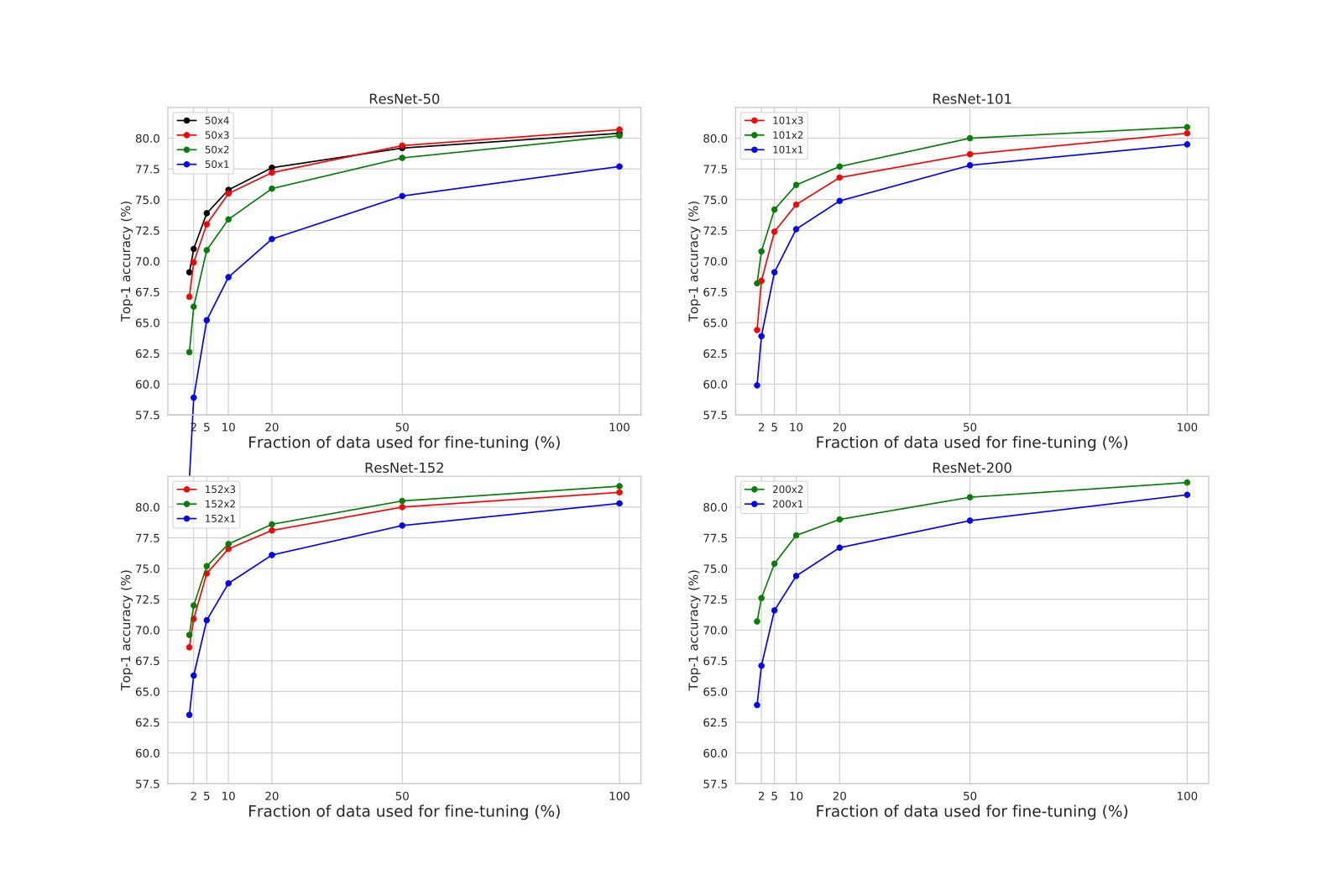
Figure 5: Semi-supervised training with a fraction of ImageNet labels on multiple ResNets architecture pretrained with BYOL. Note that large networks are facing overfitting problems.
图 5:在多种用 BYOL 预训练的 ResNet 架构上,用一部分 ImageNet 标签做半监督训练。注意大型网络面临过拟合问题。
C.2 Linear evaluation on larger architectures and supervised baselines
C.2 更大架构上的线性评估与监督基线
| BYOL | Supervised (ours) | Supervised [8] | |||||
|---|---|---|---|---|---|---|---|
| Architecture | Multiplier | Weights | Top-1 | Top-5 | Top-1 | Top-5 | Top-1 |
| ResNet-50 | 24M | ||||||
| ResNet-101 | 43M | - | |||||
| ResNet-152 | 58M | - | |||||
| ResNet-200 | 63M | - | |||||
| ResNet-50 | 94M | ||||||
| ResNet-101 | 170M | - | |||||
| ResNet-50 | 211M | - | |||||
| ResNet-152 | 232M | - | |||||
| ResNet-200 | 250M | - | |||||
| ResNet-50 | 375M | ||||||
| ResNet-101 | 382M | - | |||||
| ResNet-152 | 522M | - |
Table 9: Linear evaluation of BYOL on ImageNet using larger encoders. Top- and top- accuracies are reported in %.
Here we investigate the performance of BYOL with deeper and wider ResNet architectures. We compare ourselves to the best supervised baselines from [8] when available (rightmost column in table 9), which are also presented in Figure 1. Importantly, we close in on those baselines using the ResNet- () and the ResNet- () architectures, where we are within accuracy points of the supervised performance. To the best of our knowledge, this is the first time that the gap to supervised has been closed to such an extent using a self-supervised method under the linear evaluation protocol. Therefore, in order to ensure fair comparison, and suspecting that the supervised baselines’ performance in [8] could be even further improved with appropriate data augmentations, we also report on our own reproduction of strong supervised baselines. We use RandAugment [87] data augmentation for all large ResNet architectures (which are all version , as per [22]). We train our supervised baselines for up to epochs, using SGD with a Nesterov momentum value of , a cosine-annealed learning rate after a epochs linear warmup period, weight decay with a value of , and a label smoothing [88] value of . Results are presented in Figure 6.
这里我们研究更深更宽 ResNet 架构下 BYOL 的表现。在可用时,我们与 [8] 中最好的监督基线比较(表 9 最右列),它们也呈现在图 1 中。重要的是,在 ResNet-()与 ResNet-()架构上,我们把与监督表现的差距收窄到 个精度点以内。据我们所知,这是首次有自监督方法在线性评估协议下把与监督的差距缩小到如此程度。因此,为确保公平比较,并怀疑 [8] 中监督基线的表现若配合合适数据增强还能进一步提高,我们也报告自己复现的强监督基线。对所有大型 ResNet 架构(均为 [22] 的版本 1),我们使用 RandAugment [87] 数据增强。监督基线最多训练 个 epoch,使用动量 的 Nesterov SGD,在 个 epoch 线性预热后余弦退火学习率,权重衰减 ,标签平滑 [88] 值 。结果见图 6。
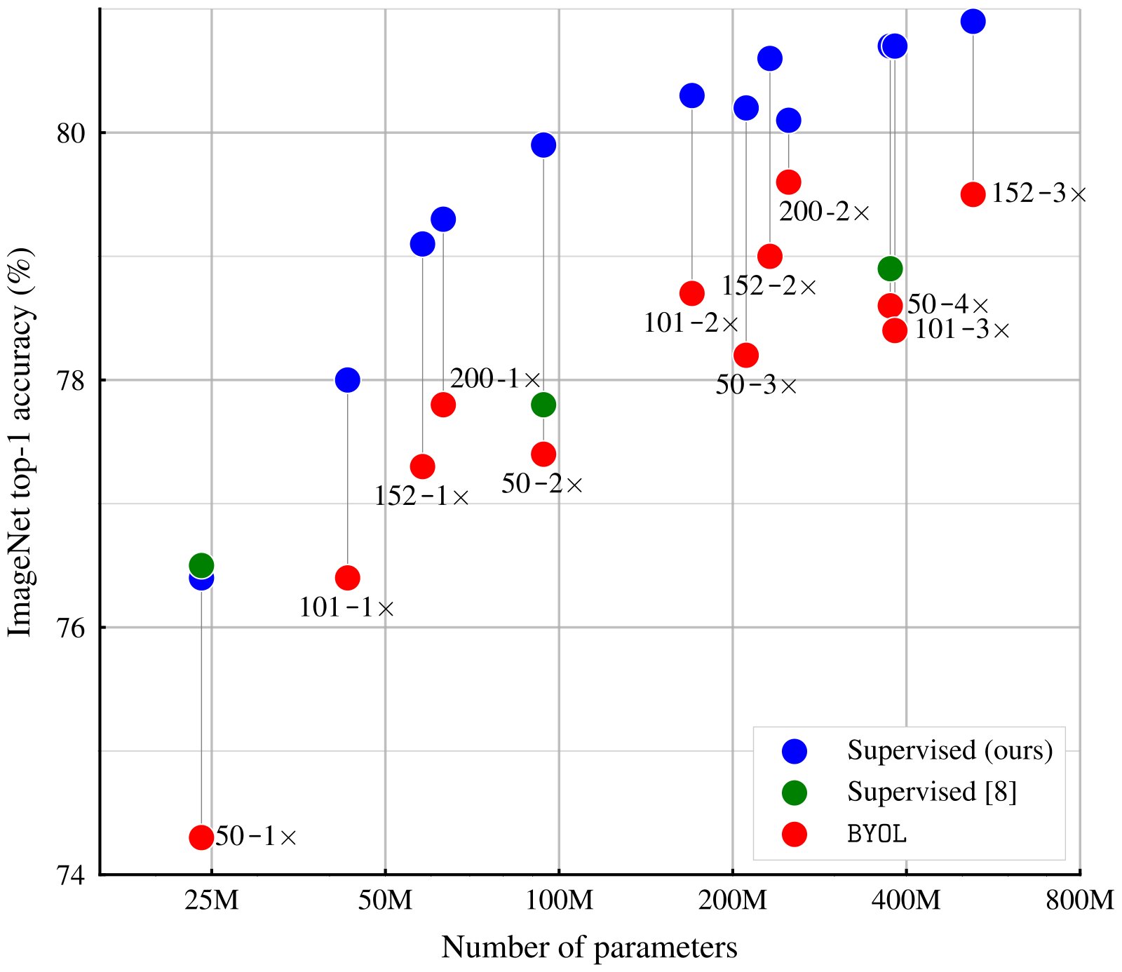
Figure 6: Results for linear evaluation of BYOL compared to fully supervised baselines with various ResNet architectures. Our supervised baselines are ran with RandAugment [87] augmentations.
图 6:多种 ResNet 架构下,BYOL 线性评估相对完全监督基线的结果。我们的监督基线使用 RandAugment [87] 增强。
Appendix D Transfer to other datasets
附录 D 迁移到其他数据集
D.1 Datasets
D.1 数据集
| Dataset | Classes | Original train examples | Train examples | Valid. examples | Test examples | Accuracy measure | Test provided |
|---|---|---|---|---|---|---|---|
| ImageNet [21] | Top-1 accuracy | - | |||||
| Food101 [89] | Top-1 accuracy | - | |||||
| CIFAR-10 [78] | Top-1 accuracy | - | |||||
| CIFAR-100 [78] | Top-1 accuracy | - | |||||
| Birdsnap [90] | Top-1 accuracy | - | |||||
| Sun397 (split 1) [79] | Top-1 accuracy | - | |||||
| Cars [91] | Top-1 accuracy | - | |||||
| Aircraft [92] | Mean per-class accuracy | Yes | |||||
| PASCAL-VOC2007 [80] | 11-point mAP / AP50 | - | |||||
| PASCAL-VOC2012 [80] | Mean IoU | - | |||||
| DTD (split 1) [81] | Top-1 accuracy | Yes | |||||
| Pets [93] | Mean per-class accuracy | - | |||||
| Caltech-101 [94] | Mean per-class accuracy | - | |||||
| Places365 [73] | Top-1 accuracy | - | |||||
| Flowers [95] | Mean per-class accuracy | Yes |
Table 10: Characteristics of image datasets used in transfer learning. When an official test split with labels is not publicly available, we use the official validation split as test set, and create a held-out validation set from the training examples.
| 数据集 | 类别数 | 原始训练样本 | 训练样本 | 验证样本 | 测试样本 | 精度指标 | 是否提供测试集 |
|---|---|---|---|---|---|---|---|
| ImageNet [21] | Top-1 精度 | - | |||||
| Food101 [89] | Top-1 精度 | - | |||||
| CIFAR-10 [78] | Top-1 精度 | - | |||||
| CIFAR-100 [78] | Top-1 精度 | - | |||||
| Birdsnap [90] | Top-1 精度 | - | |||||
| Sun397 (split 1) [79] | Top-1 精度 | - | |||||
| Cars [91] | Top-1 精度 | - | |||||
| Aircraft [92] | 每类平均精度 | Yes | |||||
| PASCAL-VOC2007 [80] | 11-point mAP / AP50 | - | |||||
| PASCAL-VOC2012 [80] | Mean IoU | - | |||||
| DTD (split 1) [81] | Top-1 精度 | Yes | |||||
| Pets [93] | 每类平均精度 | - | |||||
| Caltech-101 [94] | 每类平均精度 | - | |||||
| Places365 [73] | Top-1 精度 | - | |||||
| Flowers [95] | 每类平均精度 | Yes |
表 10:迁移学习所用图像数据集的特征。若官方带标签的测试划分未公开,我们用官方验证集作测试集,并从训练样本中划出一份留出验证集。
We perform transfer via linear classification and fine-tuning on the same set of datasets as in [8], namely Food- dataset [89], CIFAR- [78] and CIFAR- [78], Birdsnap [90], the SUN scene dataset [79], Stanford Cars [91], FGVC Aircraft [92], the PASCAL VOC classification task [80], the Describable Textures Dataset (DTD) [81], Oxford-IIIT Pets [93], Caltech- [94], and Oxford Flowers [95]. As in [8], we used the validation sets specified by the dataset creators to select hyperparameters for FGVC Aircraft, PASCAL VOC 2007, DTD, and Oxford 102 Flowers. On other datasets, we use the validation examples as test set, and hold out a subset of the training examples that we use as validation set. We use standard metrics for each datasets:
我们在与 [8] 相同的一组数据集上做线性分类与微调迁移,包括 Food- [89]、CIFAR- [78] 与 CIFAR- [78]、Birdsnap [90]、SUN 场景数据集 [79]、Stanford Cars [91]、FGVC Aircraft [92]、PASCAL VOC 分类任务 [80]、Describable Textures Dataset(DTD) [81]、Oxford-IIIT Pets [93]、Caltech- [94] 以及 Oxford Flowers [95]。与 [8] 一样,对 FGVC Aircraft、PASCAL VOC 2007、DTD 与 Oxford 102 Flowers,我们用数据集作者指定的验证集选超参。其余数据集上,把验证样本当作测试集,并从训练样本中留出子集作验证。各数据集采用标准指标:
- • Top-: We compute the proportion of correctly classified examples.
- • Top-:我们计算正确分类样本的比例。
- • Mean per class: We compute the top- accuracy for each class separately and then compute the empirical mean over the classes.
- • 类平均:我们分别计算每一类的 top- 精度,再对各类取经验均值。
- • Point 11-mAP: We compute the empirical mean average precision as defined in [80].
- • Point 11-mAP:我们计算 [80] 所定义的经验平均精度均值。
- • Mean IoU: We compute the empirical mean Intersection-Over-Union as defined in [80].
- • *Mean IoU:*我们计算 [80] 所定义的经验交并比均值。
- • AP50: We compute the Average Precision as defined in [80].
- • *AP50:*我们计算 [80] 所定义的平均精度。
We detail the validation procedures for some specific datasets:
我们对若干特定数据集的验证流程说明如下:
- • For Sun397 [79], the original dataset specifies 10 train/test splits, all of which contain 50 examples/images of 397 different classes. We use the first train/test split. The original dataset specifies no validation split and therefore, the training images have been further subdivided into 40 images per class for the train split and 10 images per class for the valid split.
- • 对 Sun397 [79],原数据集指定 10 个训练/测试划分,每个划分含 397 类、每类 50 张样本/图像。我们使用第一个训练/测试划分。原数据集未指定验证划分,因此训练图像被进一步划分为:训练划分每类 40 张,验证划分每类 10 张。
- • For Birdsnap [90], we use a random selection of valid images with the same number of images per category as the test split.
- • 对 Birdsnap [90],我们随机选取与测试划分每类图像数相同的验证图像。
- • For DTD [81], the original dataset specifies 10 train/validation/test splits, we only use the first split.
- • 对 DTD [81],原数据集指定 10 个训练/验证/测试划分,我们只使用第一个划分。
- • For Caltech-101 [94], the original does not dataset specifies any train/test splits. We have followed the approach used in [96]: This file defines datasets for 5 random splits of 25 training images per category, with 5 validation images per category and the remaining images used for testing.
- • 对 Caltech-101 [94],原数据集未指定任何训练/测试划分。我们遵循 [96] 的做法:该文件定义了 5 个随机划分,每类 25 张训练图像、5 张验证图像,其余用于测试。
- • For ImageNet, we took the last last images of the official tensorflow ImageNet split.
- • 对 ImageNet,我们取官方 tensorflow ImageNet 划分最后的 张图像。
- • For Oxford-IIIT Pets, the valid set consists of 20 randomly selected images per class.
- • 对 Oxford-IIIT Pets,验证集由每类随机选取的 20 张图像组成。
Information about the dataset are summarized in Table 10.
关于数据集的信息总结于表 10。
D.2 Transfer via linear classification
D.2 经线性分类的迁移
We follow the linear evaluation protocol of [48, 74, 8] that we detail next for completeness. We train a regularized multinomial logistic regression classifier on top of the frozen representation, i.e., with frozen pretrained parameters and without re-computing batch-normalization statistics. In training and testing, we do not perform any image augmentations; images are resized to pixels along the shorter side using bicubic resampling and then normalized with ImageNet statistics. Finally, we minimize the cross-entropy objective using LBFGS with -regularization, where we select the regularization parameters from a range of logarithmically-spaced values between and . After choosing the best-performing hyperparameters on the validation set, the model is retrained on combined training and validation images together, using the chosen parameters. The final accuracy is reported on the test set.
我们沿用 [48, 74, 8] 的线性评估协议,并在此完整写出以便对照。在冻结表征之上训练带正则的多项逻辑回归分类器,即保持预训练参数冻结,也不重新计算批归一化统计量。训练与测试均不做图像增强:图像沿较短边用双三次重采样缩到 像素,再用 ImageNet 统计量归一化。最后用带 正则的 LBFGS 最小化交叉熵,正则系数在 到 之间按对数均匀取 个候选。在验证集上选出最优超参后,用选定参数在训练+验证合并集上重训,最终在测试集上报精度。
D.3 Transfer via fine-tuning
D.3 经微调的迁移
We follow the same fine-tuning protocol as in [32, 48, 76, 8] that we also detail for completeness. Specifically, we initialize the network with the parameters of the pretrained representation. At training time, we apply spatial transformation, i.e., random crops with resize to pixels and random flips. At test time, images are resized to pixels along the shorter side using bicubic resampling, after which a center crop is extracted. In both cases, we normalize the color channels by subtracting the average color and dividing by the standard deviation (computed on ImageNet), after applying the augmentations. We optimize the loss using SGD with Nesterov momentum for steps with a batch size of and with a momentum of . We set the momentum parameter for the batch normalization statistics to where is the number of steps per epoch. The learning rate and weight decay are selected respectively with a grid of seven logarithmically spaced learning rates between and , and logarithmically-spaced values of weight decay between and , as well as no weight decay. These values of weight decay are divided by the learning rate. After choosing the best-performing hyperparameters on the validation set, the model is retrained on combined training and validation images together, using the chosen parameters. The final accuracy is reported on the test set.
我们沿用 [32, 48, 76, 8] 的微调协议并完整写出以便对照。具体地,用预训练表征参数初始化网络。训练时施加空间变换,即随机裁剪并缩放到 像素以及随机翻转。测试时,图像沿较短边用双三次重采样缩到 像素,再取 中心裁剪。两种情形下,都在增强之后按 ImageNet 均值减、标准差除做颜色通道归一化。损失用带动量 的 Nesterov SGD 优化, 步、batch size 。批归一化统计量的动量设为 ,其中 为每 epoch 步数。学习率与权重衰减分别在 – 的七个对数均匀学习率,以及 – 的七个对数均匀权重衰减(另加无权重衰减)网格上选取;这些权重衰减值再除以学习率。验证集选出最优超参后,用选定参数在训练+验证合并集上重训,最终在测试集上报精度。
D.4 Implementation details for semantic segmentation
D.4 语义分割实现细节
We use the same fully-convolutional network (FCN)-based [7] architecture as [9]. The backbone consists of the convolutional layers in ResNet-. The convolutions in the conv blocks use dilation and stride . This is followed by two extra convolutions with channels, each followed by batch normalization and ReLU activations, and a convolution for per-pixel classification. The dilation is set to in the two extra convolutions. The total stride is (FCN-s [7]).
我们采用与 [9] 相同的基于全卷积网络(FCN) [7] 的架构。骨干为 ResNet- 中的卷积层。conv 块里的 卷积使用膨胀率 、步幅 。其后接两个带 通道的额外 卷积,各自后接批归一化与 ReLU,再接一个用于逐像素分类的 卷积。这两个额外 卷积的膨胀率设为 。总步幅为 (FCN-s [7])。
We train on the train_aug2012 set and report results on val2012. Hyperparameters are selected on a images held-out validation set. We use a standard per-pixel softmax cross-entropy loss to train the FCN. Training is done with random scaling (by a ratio in \mathopen{}\mathclose{{\left[0.5,2.0}}\right]), cropping, and horizontal flipping. The crop size is . Inference is performed on the \mathopen{}\mathclose{{\left[513,513}}\right] central crop. For training we use a batch size of and weight decay of . We select the base learning rate by sweeping across logarithmically spaced values between and . The learning rate is multiplied by at the -th and -th percentile of training. We train for iterations, and average the results on 5 seeds.
我们在 train_aug2012 上训练,并在 val2012 上报结果。超参在 张留出验证图像上选取。用标准逐像素 softmax 交叉熵训练 FCN。训练时施加随机缩放(比例在 \mathopen{}\mathclose{{\left[0.5,2.0}}\right])、裁剪与水平翻转,裁剪大小为 。推理在 \mathopen{}\mathclose{{\left[513,513}}\right] 中心裁剪上进行。训练 batch size 为 ,权重衰减 。基础学习率在 与 之间五个对数均匀值上扫描;在训练进度的第 与第 百分位处学习率乘以 。共训练 次迭代,对 个随机种子取平均。
D.5 Implementation details for object detection
D.5 目标检测实现细节
For object detection, we follow prior work on Pascal detection transfer [40, 23] wherever possible. We use a Faster R-CNN [82] detector with a R-C backbone with a frozen representation. The R-C backbone ends with the conv stage of a ResNet-, and the box prediction head consists of the conv stage (including global pooling). We preprocess the images by applying multi-scale augmentation (rescaling the image so its longest edge is between and pixels) but no other augmentation. We use an asynchronous SGD optimizer with workers and train for M steps. We used an initial learning rate of , which is reduced to at 1M steps and to at M steps.
目标检测尽量沿用 Pascal 检测迁移的既有设定 [40, 23]。我们使用带冻结表征的 Faster R-CNN [82] 检测器,骨干为 R-C。R-C 骨干止于 ResNet- 的 conv 阶段,框预测头由 conv 阶段(含全局池化)组成。图像预处理只做多尺度增强(最长边缩放到 – 像素之间),不做其他增强。用 个 worker 的异步 SGD,训练 M 步。初始学习率 ,在 M 步降到 ,在 M 步降到 。
D.6 Implementation details for depth estimation
D.6 深度估计实现细节
For depth estimation, we follow the same protocol as in [83], and report its core components for completeness. We use a standard ResNet- backbone and feed the conv features into fast up-projection blocks with respective filter sizes , , , and . We use a reverse Huber loss function for training [83, 97].
对深度估计,我们遵循与 [83] 相同的协议,并为完整性报告其核心组件。我们使用标准 ResNet- 骨干,把 conv 特征送入 4 个快速上投影块,滤波器大小分别为 、、 与 。训练使用反向 Huber 损失函数 [83, 97]。
The original NYU Depth v frames of size \mathopen{}\mathclose{{\left[640,480}}\right] are down-sampled by a factor and center-cropped to \mathopen{}\mathclose{{\left[304,228}}\right] pixels. Input images are randomly horizontally flipped and the following color transformations are applied:
原始 NYU Depth v 帧尺寸为 ,先按因子 下采样,再中心裁剪到 像素。输入图像随机水平翻转,并施加如下颜色变换:
- • Grayscale with an application probability of .
- • 灰度,施加概率 。
- • Brightness with a maximum brightness difference of .
- • 亮度,最大亮度差 。
- • Saturation with a saturation factor randomly picked in the interval \mathopen{}\mathclose{{\left[0.5,1.5}}\right].
- • 饱和度,饱和度因子在区间 内随机选取。
- • Hue with a hue adjustment factor randomly picked in the interval \mathopen{}\mathclose{{\left[-0.2,0.2}}\right].
- • 色调,色调调整因子在区间 内随机选取。
We train for steps with batch size , weight decay and learning rate (scaled linearly from the setup of [83] to account for the bigger batch size).
我们训练 步,批次大小 ,权重衰减 ,学习率 (相对 [83] 的设置按更大批次线性缩放)。
D.7 Further comparisons on PASCAL and NYU v2 Depth
D.7 PASCAL 与 NYU v2 Depth 上的进一步比较
For completeness, Table 11 and 12 extends Table 4 with other published baselines which use comparable networks. We see that in almost all settings, BYOL outperforms these baselines, even when those baselines use more data or deeper models. One notable exception is RMS error for NYU Depth prediction, which is a metric that’s sensitive to outliers. The reason for this is unclear, but one possibility is that the network is producing higher-variance predictions due to being more confident about a test-set scene’s similarities with those in the training set.
为完整起见,表 11 与表 12 在表 4 之外补充了使用可比网络的其他已发表基线。几乎在所有设定下 BYOL 都优于这些基线,即便对方用了更多数据或更深模型。一个明显例外是 NYU 深度预测的 RMS 误差——该指标对异常值敏感。原因尚不清楚,一种可能是网络对测试场景与训练集相似性更有把握,从而给出方差更高的预测。
| Method | AP50 | mIoU |
|---|---|---|
| Supervised-IN [9] | ||
| RelPos [23], by [40]∗ | - | |
| Multi-task [40]∗ | - | |
| LocalAgg [98] | - | |
| MoCo [9] | ||
| MoCo + IG-1B [9] | ||
| CPC[32]∗∗ | - | |
| SimCLR (repro) | ||
| BYOL (ours) |
Table 11: Transfer results in semantic segmentation and object detection.
| 方法 | AP50 | mIoU |
|---|---|---|
| Supervised-IN [9] | ||
| RelPos [23], by [40]∗ | - | |
| Multi-task [40]∗ | - | |
| LocalAgg [98] | - | |
| MoCo [9] | ||
| MoCo + IG-1B [9] | ||
| CPC[32]∗∗ | - | |
| SimCLR(复现) | ||
| BYOL(本文) |
表 11:语义分割与目标检测上的迁移结果。
| Higher better | Lower better | ||||
|---|---|---|---|---|---|
| Method | pct. | pct. | pct. | rms | rel |
| Supervised-IN [83] | |||||
| RelPos [23], by [40]∗ | |||||
| Color [41], by [40]∗ | |||||
| Exemplar [46, 40]∗ | |||||
| Mot. Seg. [99], by [40]∗ | |||||
| Multi-task [40]∗ | |||||
| SimCLR (repro) | |||||
| BYOL (ours) |
Table 12: Transfer results on NYU v2 depth estimation.
| 越高越好 | 越低越好 | ||||
|---|---|---|---|---|---|
| 方法 | pct. | pct. | pct. | rms | rel |
| Supervised-IN [83] | |||||
| RelPos [23], by [40]∗ | |||||
| Color [41], by [40]∗ | |||||
| Exemplar [46, 40]∗ | |||||
| Mot. Seg. [99], by [40]∗ | |||||
| Multi-task [40]∗ | |||||
| SimCLR(复现) | |||||
| BYOL(本文) |
表 12:NYU v2 深度估计上的迁移结果。
Appendix E Pretraining on Places 365
附录 E 在 Places 365 上预训练
To ascertain that BYOL learns good representations on other datasets, we applied our representation learning protocol on the scene recognition dataset Places-Standard [73] before performing linear evaluation. This dataset contains million training images and validation images with labels, making it roughly similar to ImageNet in scale. We reuse the exact same parameters as in Section 4 and train the representation for epochs, using BYOL and our SimCLR reproduction. Results for the linear evaluation setup (using the protocol of Section C.1 for ImageNet and Places365, and that of Appendix D on other datasets) are reported in Table 13.
为确认 BYOL 在其他数据集上也能学到好表征,我们把同一套表征学习流程用到场景识别数据集 Places-Standard [73] 上,再做线性评估。该数据集有 百万训练图像与 张带标签验证图像,规模大致与 ImageNet 相当。我们复用第 4 节完全相同的超参,用 BYOL 与我们复现的 SimCLR 各训练 个 epoch。线性评估结果(ImageNet 与 Places365 用附录 C.1 协议,其余数据集用附录 D 协议)见表 13。
Interestingly, the representation trained by using BYOL on Places365 (BYOL-PL) consistently outperforms that of SimCLR on the same dataset, but underperforms the BYOL representation trained on ImageNet (BYOL-IN) on all tasks except Places365 and SUN397 [79], another scene understanding dataset. Interestingly, all three unsupervised representation learning methods achieve a relatively high performance on the Places365 task; for comparison, reference [73] (in its linked repository) reports a top-1 accuracy of for a ResNet-v2 trained from scratch using labels on this dataset.
有趣的是,在 Places365 上用 BYOL 训得的表征(BYOL-PL)始终优于同数据集上的 SimCLR,但在除 Places365 与另一场景理解数据集 SUN397 [79] 之外的所有任务上,都不如在 ImageNet 上训得的 BYOL(BYOL-IN)。三种无监督表征学习方法在 Places365 任务上都取得相对较高的成绩;对照地,文献 [73](其关联仓库)报告在该数据集上用标签从头训练的 ResNet-v2 top-1 精度为 。
| Method | Places365 | ImageNet | Food101 | CIFAR10 | CIFAR100 | Birdsnap | SUN397 | Cars | Aircraft | DTD | Pets | Caltech-101 | Flowers |
|---|---|---|---|---|---|---|---|---|---|---|---|---|---|
| BYOL-IN | |||||||||||||
| BYOL-PL | |||||||||||||
| SimCLR-PL |
Table 13: Transfer learning results (linear evaluation, ResNet-) from Places365 (PL). For comparison purposes, we also report the results from BYOL trained on ImageNet (BYOL-IN).
| 方法 | Places365 | ImageNet | Food101 | CIFAR10 | CIFAR100 | Birdsnap | SUN397 | Cars | Aircraft | DTD | Pets | Caltech-101 | Flowers |
|---|---|---|---|---|---|---|---|---|---|---|---|---|---|
| BYOL-IN | |||||||||||||
| BYOL-PL | |||||||||||||
| SimCLR-PL |
表 13:从 Places365(PL)出发的迁移学习结果(线性评估,ResNet-)。为对照,同时给出在 ImageNet 上训练的 BYOL(BYOL-IN)结果。
Appendix F Additional ablation results
附录 F 额外消融结果
To extend on the above results, we provide additional ablations obtained using the same experimental setup as in Section 5, i.e., 300 epochs, averaged over seeds with the initial learning rate set to , the batch size to , the weight decay to and the base target decay rate to unless specified otherwise. Confidence intervals correspond to the half-difference between the maximum and minimum score of these seeds; we omit them for half-differences lower than accuracy points.
为扩展上述结果,我们给出与第 5 节相同实验设定下的额外消融,即 个 epoch,对 个种子取平均;除非另有说明,初始学习率设为 ,batch size 为 ,权重衰减为 ,基础目标衰减率 为 。置信区间取这些种子最高分与最低分之差的一半;半差低于 个精度点时省略。
F.1 Architecture settings
F.1 架构设置
Table 14 shows the influence of projector and predictor architecture on BYOL. We examine the effect of different depths for both the projector and predictor, as well as the effect of the projection size. We do not apply a ReLU activation nor a batch normalization on the final linear layer of our MLPs such that a depth of corresponds to a linear layer. Using the default projector and predictor of depth yields the best performance.
表 14 展示投影器与预测器架构对 BYOL 的影响。我们考察二者不同深度以及投影维度的效果。MLP 最后一层线性层不加 ReLU,也不加批归一化,因此深度为 即对应单层线性层。默认投影器与预测器深度均为 时效果最好。
| Proj. depth | Pred. depth | Top- | Top- |
|---|---|---|---|
(a) Projector and predictor depth (i.e. the number of Linear layers).
| 投影器 深度 | 预测器 深度 | Top- | Top- |
|---|---|---|---|
(a) 投影器与预测器深度(即 Linear 层数)。
Table 15(a) shows the influence of the initial learning rate on BYOL. Note that the optimal value depends on the number of training epochs. Table 15(b) displays the influence of the weight decay on BYOL.
表 15(a) 显示初始学习率对 BYOL 的影响。注意最优值依赖训练 epoch 数。表 15(b) 显示权重衰减对 BYOL 的影响。
| Learning | ||
|---|---|---|
| rate | Top- | Top- |
| Weight decay coefficient | Top- | Top- |
|---|---|---|
(a) Base learning rate.
| 学习 | ||
|---|---|---|
| 率 | Top- | Top- |
| 权重衰减系数 | Top- | Top- |
|---|---|---|
(a) 基础学习率。
F.2 Batch size
F.2 批次大小
We run a sweep over the batch size for both BYOL and our reproduction of SimCLR. As explained in Section 5, when reducing the batch size by a factor , we average gradients over consecutive steps and update the target network once every steps. We report in Table 16, the performance of both our reproduction of SimCLR and BYOL for batch sizes between (BYOL and SimCLR default) down to . We observe that the performance of SimCLR deteriorates faster than the one of BYOL which stays mostly constant for batch sizes larger than . We believe that the performance at batch size could match the performance of the large batch size with proper parameter tuning when accumulating the gradient. We think that the drop in performance at batch size in table 16 is mainly related to the ill behaviour of batch normalization at low batch sizes [100].
我们对 BYOL 与复现的 SimCLR 扫了一遍 batch size。如第 5 节所述,当 batch size 缩小 倍时,我们在连续 步上平均梯度,并每 步更新一次目标网络。表 16 给出 batch size 从 (BYOL 与 SimCLR 默认)降到 时二者的表现。可见 SimCLR 掉点更快,而 BYOL 在 batch size 大于 时大体保持平稳。我们相信,若在梯度累积时仔细调参,batch size 有望追上大 batch 的成绩。表 16 中 batch size 的掉点,我们主要归因于小 batch 下批归一化行为不良 [100]。
| Batch | Top- | Top- | ||
|---|---|---|---|---|
| size | BYOL (ours) | SimCLR (repro) | BYOL (ours) | SimCLR (repro) |
Table 16: Influence of the batch size.
| Batch | Top- | Top- | ||
|---|---|---|---|---|
| size | BYOL(本文) | SimCLR(复现) | BYOL(本文) | SimCLR(复现) |
表 16:batch size 的影响。
F.3 Image augmentations
F.3 图像增强
Table 17 compares the impact of individual image transformations on BYOL and SimCLR. BYOL is more resilient to changes of image augmentations across the board. For completeness, we also include an ablation with symmetric parameters across both views; for this ablation, we use a Gaussian blurring w.p. of and a solarization w.p. of for both and , and recover very similar results compared to our baseline choice of parameters.
表 17 比较单项图像变换对 BYOL 与 SimCLR 的影响。总体而言 BYOL 对增强变化更稳健。为完整起见,我们也给出两视图对称参数的消融:对 与 均以 概率做高斯模糊、以 概率做日晒化,结果与基线参数选择非常接近。
| Top- | Top- | |||
|---|---|---|---|---|
| Image augmentation | BYOL (ours) | SimCLR (repro) | BYOL (ours) | SimCLR (repro) |
| Baseline | ||||
| Remove flip | ||||
| Remove blur | ||||
| Remove color (jittering and grayscale) | ||||
| Remove color jittering | ||||
| Remove grayscale | ||||
| Remove blur in | ||||
| Remove solarize in | ||||
| Remove blur and solarize in | ||||
| Symmetric blurring/solarization | ||||
| Crop only | ||||
| Crop and flip only | ||||
| Crop and color only | ||||
| Crop and blur only |
Table 17: Ablation on image transformations.
| Top- | Top- | |||
|---|---|---|---|---|
| 图像增强 | BYOL(本文) | SimCLR(复现) | BYOL(本文) | SimCLR(复现) |
| 基线 | ||||
| 去掉翻转 | ||||
| 去掉模糊 | ||||
| 去掉颜色(抖动与灰度) | ||||
| 去掉颜色抖动 | ||||
| 去掉灰度 | ||||
| 在 中去掉模糊 | ||||
| 在 中去掉日晒化 | ||||
| 在 中去掉模糊与日晒化 | ||||
| 对称模糊/日晒化 | ||||
| 仅裁剪 | ||||
| 仅裁剪与翻转 | ||||
| 仅裁剪与颜色 | ||||
| 仅裁剪与模糊 |
表 17:图像变换消融。
| Loss weight | Temperature | Top- | Top- |
|---|---|---|---|
Table 18: Top-1 accuracy in % under linear evaluation protocol at 300 epochs of sweep over the temperature and the dispersion term weight when using a predictor and a target network.
| 损失权重 | 温度 | Top- | Top- |
|---|---|---|---|
表 18:在使用预测器与目标网络时,对温度 与分散项权重 做扫描, 个 epoch 线性评估下的 Top-1 精度(%)。
F.4 Details on the relation to contrastive methods
F.4 与对比方法关系的细节
As mentioned in Section 5, the BYOL loss Equation 2 can be derived from the InfoNCE loss
如第 5 节所述,BYOL 损失(方程 2)可由 InfoNCE 损失导出
\text{InfoNCE}^{\alpha,\beta}_{{\theta}}\mathrel{\hbox{\hskip 3.8889pt\hskip-3.8889pt\hbox{$=$}\hskip-3.8889pt\hskip-2.7431pt\raisebox{4.66875pt}{\hbox{$\scriptscriptstyle\Delta$}}\hskip-2.7431pt\hskip 3.8889pt}}\frac{2}{B}\sum_{i=1}^{B}S_{\theta}(v_{i},v^{\prime}_{i})\!-\!\frac{2\alpha\cdot\beta}{B}\sum_{i=1}^{B}\ln\mathopen{}\mathclose{{\left(\sum\limits_{j\neq i}\exp\frac{S_{\theta}(v_{i},v_{j})}{\alpha}+\sum\limits_{j}\exp\frac{S_{\theta}(v_{i},v^{\prime}_{j})}{\alpha}}}\right)\mathbin{\raisebox{2.15277pt}{,}} \tag{8}
with
其中
The InfoNCE loss, introduced in [10], can be found in factored form in [84] as
InfoNCE 损失由 [10] 引入,可在 [84] 中找到因式形式
As in SimCLR [8] we also use negative examples given by to get
与 SimCLR [8] 一样,我们也使用由 给出的负例,从而得到
\displaystyle\frac{1}{B}\sum_{i=1}^{B}\ln\cfrac{\exp f(v_{i},v^{\prime}_{i})}{\frac{1}{B}\sum\limits_{j\neq i}\exp f(v_{i},v_{j})+\frac{1}{B}\sum\limits_{j}\exp f(v_{i},v^{\prime}_{j})} \\ \displaystyle\qquad=\ln B+\frac{1}{B}\sum_{i=1}^{B}f(v_{i},v^{\prime}_{i})-\frac{1}{B}\sum_{i=1}^{B}\ln\mathopen{}\mathclose{{\left(\sum\limits_{j\neq i}\exp f(v_{i},v_{j})+\sum\limits_{j}\exp f(v_{i},v^{\prime}_{j})}}\right). \tag{11}
To obtain Equation 8 from Equation 12, we subtract (which is independent of ), multiply by , take and finally multiply the second (negative examples) term by . Using and dividing by gets us back to the usual InfoNCE loss as used by SimCLR.
为从方程 12 得到方程 8,我们减去 (与 无关),乘以 ,取 ,最后把第二项(负例项)乘以 。取 并除以 ,即回到 SimCLR 所用的常规 InfoNCE 损失。
In our ablation in Table 5(b), we set the temperature to its best value in the SimCLR setting (i.e., ). With this value, setting to 1 (which adds negative examples), in the BYOL setting (i.e., with both a predictor and a target network) hurts the performances. In Table 18, we report results of a sweep over both the temperature and the weight parameter with a predictor and a target network where BYOL corresponds to . No run significantly outperforms BYOL and some values of and hurt the performance. While the best temperature for SimCLR (without the target network and a predictor) is , after adding a predictor and a target network the best temperature is higher than .
在表 5(b) 的消融中,我们把温度 设为 SimCLR 设定下的最优值(即 )。在该取值下,把 设为 (即加入负样本),在 BYOL 设定(同时有预测器与目标网络)中会伤害性能。表 18 报告在同时使用预测器与目标网络时对温度 与权重参数 的扫描结果,其中 BYOL 对应 。没有任何一组显著超过 BYOL,部分 与 还会掉点。SimCLR(无目标网络、无预测器)的最佳温度是 ,加入预测器与目标网络后,最佳温度 高于 。
Using a target network in the loss has two effects: stopping the gradient through the prediction targets and stabilizing the targets with averaging. Stopping the gradient through the target change the objective while averaging makes the target stable and stale. In Table 5(b) we only shows results of the ablation when either using the online network as the prediction target (and flowing the gradient through it) or with a target network (both stopping the gradient into the prediction targets and computing the prediction targets with a moving average of the online network). We shown in Table 5(b) that using a target network is beneficial but it has two distinct effects we would like to understand from which effect the improvement comes from. We report in Table 19 the results already in Table 5(b) but also when the prediction target is computed with a stop gradient of the online network (the gradient does not flow into the prediction targets). This shows that making the prediction targets stable and stale is the main cause of the improvement rather than the change in the objective due to the stop gradient.
在损失里使用目标网络有两重效果:截断经预测目标的梯度,以及用平均使目标稳定。截断梯度会改变目标函数,平均则让目标稳定且“陈旧”。表 5(b) 只给出两类消融:要么用在线网络作预测目标(梯度穿过去),要么用目标网络(既截断进入预测目标的梯度,又用在线网络的滑动平均算预测目标)。表 5(b) 表明使用目标网络有益,但这两种效果混在一起,我们想弄清增益主要来自哪一种。表 19 在表 5(b) 已有结果之外,补充了用在线网络的停梯度作为预测目标(梯度不流入预测目标)的情形。结果表明:让预测目标稳定且陈旧,才是主要增益来源,而不是停梯度带来的目标函数变化。
| Method | Predictor | Target parameters | Top-1 | |
|---|---|---|---|---|
| BYOL | ✓ | 0 | ||
| ✓ | 1 | |||
| 1 | ||||
| ✓ | 1 | |||
| SimCLR | 1 | |||
| ✓ | 1 | |||
| 1 | ||||
| ✓ | 1 | |||
| ✓ | 0 | |||
| ✓ | 0 | |||
| 0 | ||||
| 0 | ||||
| 0 |
Table 19: Top-1 accuracy in %, under linear evaluation protocol at 300 epochs, of intermediate variants between BYOL and SimCLR (with caveats discussed in Section F.5). means stop gradient.
| 方法 | 预测器 | 目标参数 | Top-1 | |
|---|---|---|---|---|
| BYOL | ✓ | 0 | ||
| ✓ | 1 | |||
| 1 | ||||
| ✓ | 1 | |||
| SimCLR | 1 | |||
| ✓ | 1 | |||
| 1 | ||||
| ✓ | 1 | |||
| ✓ | 0 | |||
| ✓ | 0 | |||
| 0 | ||||
| 0 | ||||
| 0 |
表 19:在 BYOL 与 SimCLR 之间的中间变体在 个 epoch 线性评估下的 Top-1 精度(%)(附带第 F.5 节讨论的注意点)。 表示停梯度。
F.5 SimCLR baseline of Section 5
F.5 第 5 节的 SimCLR 基线
The SimCLR baseline in Section 5 (, without predictor nor target network) is slightly different from the original one in [8]. First we multiply the original loss by . For comparaison here is the original SimCLR loss,
第 5 节中的 SimCLR 基线(,无预测器也无目标网络)与 [8] 中的原始版本略有不同。首先我们把原始损失乘以 。为便于比较,这里给出原始 SimCLR 损失,
\displaystyle\text{InfoNCE}_{{\theta}}\mathrel{\hbox{\hskip 3.8889pt\hskip-3.8889pt\hbox{$=$}\hskip-3.8889pt\hskip-2.7431pt\raisebox{4.66875pt}{\hbox{$\scriptscriptstyle\Delta$}}\hskip-2.7431pt\hskip 3.8889pt}}\frac{1}{B}\sum_{i=1}^{B}\frac{S_{\theta}(v_{i},v^{\prime}_{i})}{\alpha}\!-\!\frac{1}{B}\sum_{i=1}^{B}\ln\mathopen{}\mathclose{{\left(\sum\limits_{j\neq i}\exp\frac{S_{\theta}(v_{i},v_{j})}{\alpha}+\sum\limits_{j}\exp\frac{S_{\theta}(v_{i},v^{\prime}_{j})}{\alpha}}}\right)\cdot \tag{13}
Note that this multiplication by matters as the LARS optimizer is not completely invariant with respect to the scale of the loss. Indeed, LARS applies a preconditioning to gradient updates on all weights, except for biases and batch normalization parameters. Updates on preconditioned weights are invariant by multiplicative scaling of the loss. However, the bias and batch normalization parameter updates remain sensitive to multiplicative scaling of the loss.
注意:乘以 是有意义的,因为 LARS 优化器对损失尺度并非完全不变。LARS 会对除偏置与批归一化参数以外的所有权重做预条件更新;经预条件的权重更新对损失的乘性缩放不变。但偏置与批归一化参数的更新仍对损失的乘性缩放敏感。
We also increase the original SimCLR hidden and output size of the projector to respectively 4096 and 256. In our reproduction of SimCLR, these three combined changes improves the top-1 accuracy at 300 epochs from (without the changes) to (with the changes).
我们还将原始 SimCLR 投影器的隐层与输出尺寸分别增大到 4096 与 256。在我们复现的 SimCLR 中,这三项改动合起来把 300 个 epoch 时的 top-1 精度从 (无改动)提升到 (有改动)。
F.6 Ablation on the normalization in the loss function
F.6 损失函数中归一化的消融
(a) Representation -norm
(a) 表征 -范数
| Normalization | Top-1 | Top-5 |
|---|---|---|
| -norm | ||
| LayerNorm | ||
| No normalization | ||
| BatchNorm |
Table 20: Top-1 accuracy in % under linear evaluation protocol at 300 epochs for different normalizations in the loss.
| 归一化 | Top-1 | Top-5 |
|---|---|---|
| -范数 | ||
| LayerNorm | ||
| 无归一化 | ||
| BatchNorm |
表 20:损失中不同归一化下,300 个 epoch 线性评估协议的 Top-1 精度(%)。
BYOL minimizes a squared error between the -normalized prediction and target. We report results of BYOL at 300 epochs using different normalization function and no normalization at all. More precisely, given batch of prediction and targets in , with the batch size, BYOL uses the loss function with . We run BYOL with other normalization functions: non-trainable batch-normalization and layer-normalization and no normalization. We divide the batch normalization and layer normalization by to have a consistent scale with the -normalization. We report results in Table 20 where , LayerNorm, no normalization and BatchNorm respectively denote using , , and with
BYOL 最小化 归一化后的预测与目标之间的平方误差。我们报告 个 epoch 下改用其他归一化函数、乃至完全不做归一化的结果。更精确地,给定批次内的预测与目标 ( 为 batch size),BYOL 使用损失 ,其中 。我们还试验了不可训练的批归一化、层归一化以及无归一化。批归一化与层归一化再除以 ,以与 归一化尺度一致。结果见表 20,其中 、LayerNorm、无归一化与 BatchNorm 分别对应 、、 与 ,且
\displaystyle{n_{\text{{B\hskip-0.70004ptN} }}^{j}}_{i} \\ \displaystyle:x\rightarrow\frac{x_{i}^{j}-\mu_{\text{{B\hskip-0.70004ptN} }}^{j}(x)}{\sigma_{\text{BN}}^{j}(x)\cdot\sqrt{d}}\mathbin{\raisebox{2.15277pt}{,}}\quad{n_{\text{{L\hskip-0.70004ptN} }}^{j}}_{i}:x\rightarrow\frac{x_{i}^{j}-{\mu_{\text{{L\hskip-0.70004ptN} }}}_{i}(x)}{{\sigma_{\text{LN}}}_{i}(x)\cdot\sqrt{d}}\mathbin{\raisebox{2.15277pt}{,}}\quad n_{\text{{I\hskip-0.70004ptd} }}:x\rightarrow x, \\ \displaystyle\mu_{\text{{B\hskip-0.70004ptN} }}^{j} \\ \displaystyle:x\rightarrow\frac{1}{B}\sum_{i=1}^{B}x_{i}^{j},\quad\sigma_{\text{{B\hskip-0.70004ptN} }}^{j}:x\rightarrow\sqrt{\frac{1}{B}\sum_{i=1}^{B}\mathopen{}\mathclose{{\left({x_{i}^{j}}}}\right)^{2}-\mu_{\text{{B\hskip-0.70004ptN} }}^{j}(x)^{2}},\quad \\ \displaystyle{\mu_{\text{{L\hskip-0.70004ptN} }}}_{i} \\ \displaystyle:x\rightarrow\frac{1}{d}\sum_{j=1}^{d}x_{i}^{j},\quad{\sigma_{\text{{L\hskip-0.70004ptN} }}}_{i}:x\rightarrow\frac{\|x_{i}-{\mu_{\textsc{L\hskip-0.70004ptN}}}_{i}(x)\|_{2}}{\sqrt{d}}
When using no normalization at all, the projection norm rapidly increases during the first 100 epochs and stabilizes at around as shown in Figure 7. Despite this behaviour, using no normalization still performs reasonably well . The normalization performs the best.
完全不使用归一化时,投影的 范数在前 100 个 epoch 迅速增大,并稳定在约 ,如图 7 所示。尽管如此,无归一化仍有合理表现()。 归一化表现最好。
Appendix G Training with smaller batch sizes
附录 G 用更小批次训练
The results described in Section 4 were obtained using a batch size of split over TPU cores. Due to its increased robustness, BYOL can also be trained using smaller batch sizes without significantly decreasing performance. Using the same linear evaluation setup, BYOL achieves top-1 accuracy when trained over epochs with a batch size of split over TPU cores (approximately days of training). For this setup, we reuse the same setting as in Section 3, but use a base learning rate of (appropriately scaled by the batch size) and with the same weight decay coefficient of .
第 4 节结果使用 batch size ,分在 个 TPU 核上。由于鲁棒性更强,BYOL 也能用更小 batch 训练而不显著掉点。同一线性评估设定下,用 batch size 分在 个 TPU 核上训练 个 epoch(约 天),BYOL 取得 top-1 精度。该设定复用第 3 节其余配置,但基础学习率取 (按 batch size 适当缩放),,权重衰减系数仍为 。
Appendix H Details on Equation 5 in Section 3.2
附录 H 第 3.2 节方程 5 的细节
In this section we clarify why BYOL’s update is related to Equation 5 from Section 3.2,
本节澄清为何 BYOL 的更新与第 3.2 节方程 5 相关,
\displaystyle\nabla_{\theta}\mathbb{E}\mathopen{}\mathclose{{\left[\mathopen{}\mathclose{{\left\|q^{\star}(z_{\theta})-z^{\prime}_{\xi}}}\right\|_{2}^{2}}}\right]=\nabla_{\theta}\mathbb{E}\mathopen{}\mathclose{{\left[\mathopen{}\mathclose{{\left\|\mathbb{E}\mathopen{}\mathclose{{\left[z^{\prime}_{\xi}|z_{\theta}}}\right]-z^{\prime}_{\xi}}}\right\|_{2}^{2}}}\right]=\nabla_{\theta}\mathbb{E}\mathopen{}\mathclose{{\left[\sum_{i}\var(z^{\prime}_{\xi,i}|z_{\theta})}}\right]. \tag{5}
Recall that is defined as
回顾 定义为
\displaystyle q^{\star}\mathrel{\hbox{\hskip 3.8889pt\hskip-3.8889pt\hbox{$=$}\hskip-3.8889pt\hskip-2.7431pt\raisebox{4.66875pt}{\hbox{$\scriptscriptstyle\Delta$}}\hskip-2.7431pt\hskip 3.8889pt}}\argmin_{q}\mathbb{E}\mathopen{}\mathclose{{\left[\mathopen{}\mathclose{{\left\|q(z_{\theta})-z^{\prime}_{\xi}}}\right\|_{2}^{2}}}\right],\quad\text{where}\quad q^{\star}(z_{\theta})=\mathbb{E}\mathopen{}\mathclose{{\left[z^{\prime}_{\xi}|z_{\theta}}}\right], \tag{4}
and implicitly depends on and ; therefore, it should be denoted as instead of just . For simplicity we write as the output of the optimal predictor for any parameters and and input .
并且它隐式依赖 与 ;因此应记为 而非仅 。为简洁起见,对任意参数 、 与输入 ,我们把最优预测器的输出 写作 。
BYOL updates its online parameters following the gradient of Equation 5, but considering only the gradients of with respect to its third argument when applying the chain rule. If we rewrite
BYOL 按方程 5 的梯度更新在线参数,但在应用链式法则时,只考虑 相对其第三个自变量 的梯度。若我们重写
\displaystyle\mathbb{E}\mathopen{}\mathclose{{\left[\mathopen{}\mathclose{{\left\|q^{\star}({\theta},\xi,z_{\theta})-z^{\prime}_{\xi}}}\right\|_{2}^{2}}}\right]=\mathbb{E}\mathopen{}\mathclose{{\left[L(q^{\star}({\theta},\xi,z_{\theta}),z^{\prime}_{\xi})}}\right], \tag{14}
the gradient of this quantity w.r.t. is
该量相对 的梯度为
\displaystyle\frac{\partial}{\partial{\theta}}\mathbb{E}\mathopen{}\mathclose{{\left[L(q^{\star}({\theta},\xi,z_{\theta}),z^{\prime}_{\xi})}}\right]=\mathbb{E}\mathopen{}\mathclose{{\left[\frac{\partial L}{\partial q}\cdot\frac{\partial q^{\star}}{\partial{\theta}}+\frac{\partial L}{\partial q}\cdot\frac{\partial q^{\star}}{\partial z}\cdot\frac{\partial z_{\theta}}{\partial{\theta}}}}\right], \tag{15}
where and are the gradients of with respect to its first and last argument. Using the envelope theorem, and thanks to the optimality condition of the predictor, the term \mathbb{E}\mathopen{}\mathclose{{\left[\frac{\partial L}{\partial q}\cdot\frac{\partial q^{\star}}{\partial{\theta}}}}\right]=0. Therefore, the remaining term \mathbb{E}\mathopen{}\mathclose{{\left[\frac{\partial L}{\partial q}\cdot\frac{\partial q^{\star}}{\partial z}\cdot\frac{\partial z_{\theta}}{\partial{\theta}}}}\right] where gradients are only back-propagated through the predictor’s input is exactly the direction followed by BYOL.
其中 与 是 对其第一与最后一个参数的梯度。由包络定理,并借助预测器的最优性条件,项 \mathbb{E}\mathopen{}\mathclose{{\left[\frac{\partial L}{\partial q}\cdot\frac{\partial q^{\star}}{\partial{\theta}}}}\right]=0。因此,剩余项 \mathbb{E}\mathopen{}\mathclose{{\left[\frac{\partial L}{\partial q}\cdot\frac{\partial q^{\star}}{\partial z}\cdot\frac{\partial z_{\theta}}{\partial{\theta}}}}\right]——梯度只经预测器输入回传——正是 BYOL 所沿的方向。
Appendix I Importance of a near-optimal predictor
附录 I 接近最优的预测器的重要性
In this part we build upon the intuitions of Section 3.2 on the importance of keeping the predictor near-optimal. Specifically, we show that it is possible to remove the exponential moving average in BYOL’s target network (i.e., simply copy weights of the online network into the target) without causing the representation to collapse, provided the predictor remains sufficiently good.
本部分建立在第 3.2 节关于保持预测器接近最优之重要性的直觉之上。具体地,我们表明:只要预测器保持足够好,就有可能去掉 BYOL 目标网络中的指数滑动平均(即简单地把在线网络权重复制到目标网络),而不导致表征崩塌。
I.1 Predictor learning rate
I.1 预测器学习率
In this setup, we remove the exponential moving average (i.e., set over the full training in Equation 1), and multiply the learning rate of the predictor by a constant compared to the learning rate used for the rest of the network; all other hyperparameters are unchanged. As shown in Table 21, using sufficiently large values of provides a reasonably good level of performance and the performance sharply decreases with to top-1 accuracy (no better than random) for .
该设定下去掉指数滑动平均(即在式 1 的全程训练中令 ),并把预测器学习率相对网络其余部分乘以常数 ;其余超参不变。如表 21 所示, 足够大时仍能达到尚可的水平,而随 降到 ,性能急剧掉到 top-1(不优于随机)。
To show that this effect is directly related to a change of behavior in the predictor, and not only to a change of learning rate in any subpart of the network, we perform a similar experiment by using a multiplier on the predictor’s learning rate, and a different multiplier for the projector. In Table 22, we show that the representation typically collapses or performs poorly when the predictor learning rate is lower or equal to that of the projector. As mentioned in Section 3.2, we further hypothesize that one of the contributions of the target network is to maintain a near optimal predictor at all times.
为说明这一效应直接来自预测器行为变化,而不只是网络某一子模块学习率变了,我们做类似实验:对预测器学习率乘 ,对投影器另乘 。表 22 表明,当预测器学习率低于或等于投影器时,表征通常崩塌或表现很差。如第 3.2 节所述,我们进一步猜想:目标网络的贡献之一,正是始终维持接近最优的预测器。
I.2 Optimal linear predictor in closed form
I.2 闭式最优线性预测器
Similarly, we can get rid of the slowly moving target network if we use a closed form optimal predictor on the batch, instead of a learned, non-optimal one. In this case we restrict ourselves to a linear predictor,
类似地,若在批次上使用闭式最优预测器,而不是学到的、非最优预测器,我们也可以去掉慢速滑动的目标网络。此时我们把自身限制为线性预测器,
\displaystyle q^{\star}=\argmin_{Q}\mathopen{}\mathclose{{\left\|Z_{\theta}Q-Z^{\prime}_{\xi}}}\right\|_{2}^{2}=\mathopen{}\mathclose{{\left(Z_{\theta}^{\mathsf{\scriptscriptstyle T}}Z_{\theta}}}\right)^{-1}Z_{\theta}^{\mathsf{\scriptscriptstyle T}}Z^{\prime}_{\xi}
with \mathopen{}\mathclose{{\left\|\cdot}}\right\|_{2} being the Frobenius norm, and of shape respectively the online and target projections, where is the batch size and the number of features; and of shape , the optimal linear predictor for the batch.
其中 为 Frobenius 范数, 与 形状为 ,分别是在线与目标投影, 为批次大小, 为特征数; 形状为 ,是该批次的最优线性预测器。
At epochs, when using the closed form optimal predictor, and directly hard copying the weights of the online network into the target, we obtain a top- accuracy of .
在 个 epoch 时,使用闭式最优预测器并把在线网络权重直接硬拷贝到目标网络,我们获得的 top- 精度为 fill。
| Top- | |
|---|---|
| Baseline |
Table 21: Top- accuracy at 300 epochs when removing the slowly moving target network, directly hard copying the weights of the online network into the target network, and applying a multiplier to the predictor learning rate.
| Top- | |
|---|---|
| 基线 |
表 21:去掉慢速滑动目标网络、把在线网络权重硬拷贝到目标网络,并对预测器学习率施加乘数时, 个 epoch 的 Top- 精度。
Table 22: Top- accuracy at 300 epochs when removing the slowly moving target network, directly hard copying the weights of the online network in the target network, and applying a multiplier to the projector and to the predictor learning rate. The predictor learning rate needs to be higher than the projector learning rate in order to successfully remove the target network. This further suggests that the learning dynamic of predictor is central to BYOL’s stability.
表 22:去掉慢速滑动目标网络、把在线网络权重硬拷贝到目标网络,并对投影器施加乘数 、对预测器施加乘数 时, 个 epoch 的 Top- 精度。要成功去掉目标网络,预测器学习率需高于投影器学习率。这进一步表明预测器的学习动态对 BYOL 的稳定性至关重要。
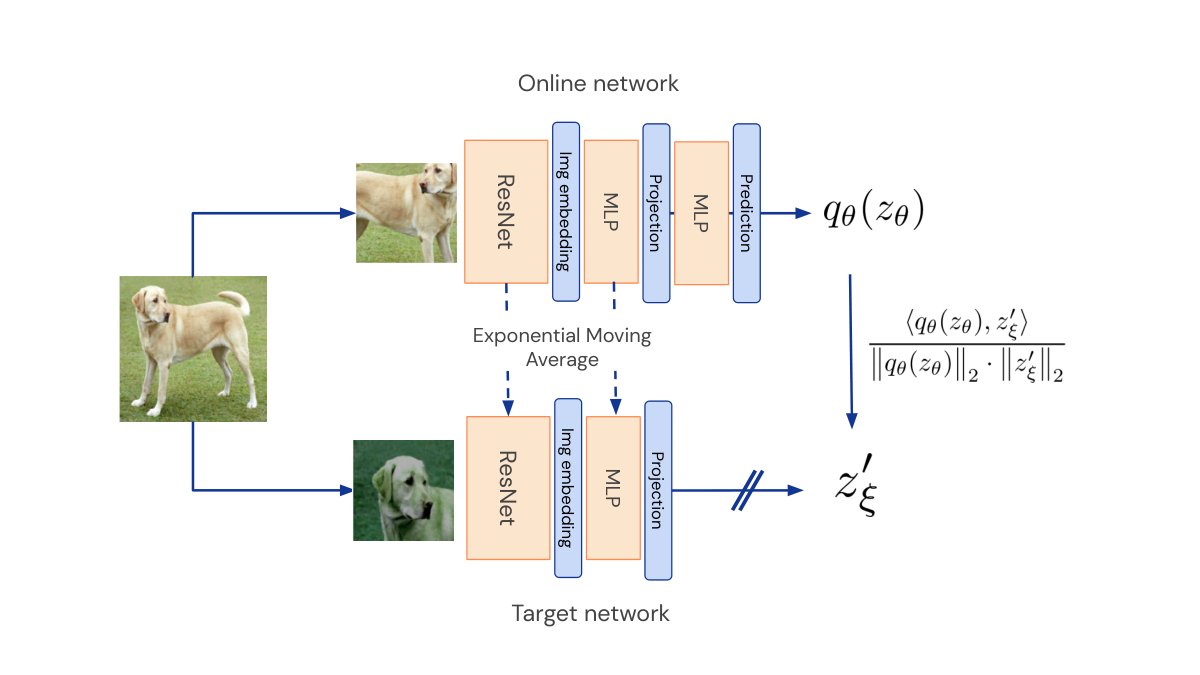
Figure 8: BYOL sketch summarizing the method by emphasizing the neural architecture.
图 8:通过强调神经网络架构来概括方法的 BYOL 示意图。
See pages 1-3 of lalala.pdf
见 lalala.pdf 第 1–3 页。