Building Rome with Convex Optimization
Building Rome with Convex Optimization
用凸优化建造罗马
Haoyu Han and Heng Yang Affiliation: School of Engineering and Applied Sciences, Harvard University Affiliation: https://computationalrobotics.seas.harvard.edu/XM
Abstract
摘要
Global bundle adjustment is made easy by depth prediction and convex optimization. We (i) propose a scaled bundle adjustment (SBA) formulation that lifts 2D keypoint measurements to 3D with learned depth, (ii) design an empirically tight convex semidefinite programming (SDP) relaxation that solves SBA to certifiable global optimality, (iii) solve the SDP relaxation at extreme scale with Burer-Monteiro factorization and a CUDA-based trust-region Riemannian optimizer (dubbed XM), (iv) build a structure from motion pipeline with XM as the optimization engine and show that XM-SfM compares favorably with existing pipelines in terms of reconstruction quality while being significantly faster, more scalable, and initialization-free.
全局束调整因深度预测与凸优化而变得容易。我们 (i) 提出缩放束调整(SBA)公式,用学习深度把二维关键点测量提升到三维;(ii) 设计经验上紧的凸半定规划(SDP)松弛,以可证明的全局最优性求解 SBA;(iii) 用 Burer-Monteiro 分解与基于 CUDA 的信赖域黎曼优化器(称为 XM)在极端规模上求解 SDP 松弛;(iv) 以 XM 为优化引擎构建运动恢复结构管线,并表明 XM-SfM 在重建质量上可与现有管线媲美,同时显著更快、更可扩展,且无需初始化。
(a) BAL Dataset. From left to right: , , and camera frames.
(a) BAL 数据集。从左到右:、 与 个相机帧。
(b) Replica Dataset. All three cases have camera frames.
(b) Replica 数据集。三种情形均有 个相机帧。
(c) Mip-Nerf Dataset (left: reconstruction, right: novel view synthesis). camera frames.
(c) Mip-Nerf 数据集(左:重建,右:新视角合成)。 个相机帧。
(d) IMC Dataset. From left to right: , , and camera frames.
(d) IMC 数据集。从左到右:、 与 个相机帧。
Left (e) TUM Dataset ( and camera frames); Right (f) C3VD Dataset ( and camera frames).
左 (e) TUM 数据集( 与 个相机帧);右 (f) C3VD 数据集( 与 个相机帧)。
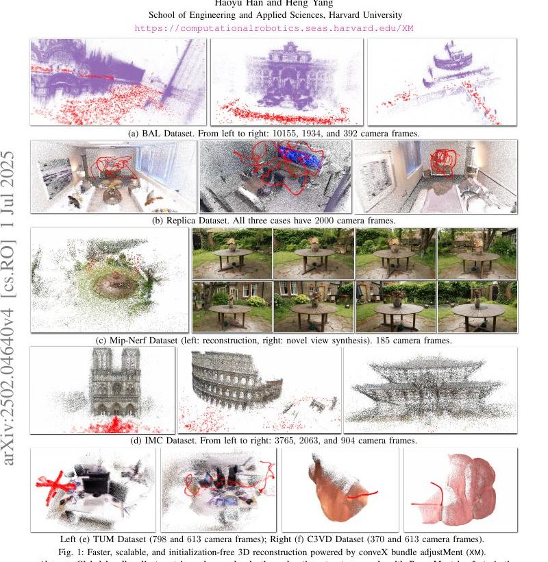
Fig. 1: Faster, scalable, and initialization-free 3D reconstruction powered by conveX bundle adjustMent (XM).
图 1:由 conveX bundle adjustMent(XM)驱动的更快、可扩展且无需初始化的三维重建。
I Introduction
I 引言
At the heart of modern structure from motion (SfM) and simultaneous localization and mapping (SLAM) sits bundle adjustment (BA), the procedure of reconstructing camera poses and 3D landmarks from 2D image keypoints.
现代运动恢复结构(SfM)与同时定位与建图(SLAM)的核心是束调整(BA):从二维图像关键点重建相机位姿与三维路标。
Classical BA formulation. Consider a so-called view graph illustrated in Fig. 2 with two types of nodes: 3D points and camera poses . The set of edges contains visibility information. An edge indicates the -th 3D point is visible to the -th camera, and a 2D keypoint measurement has been obtained regarding the projection of the point onto the camera frame.[^1] The bundle adjustment problem consists of estimating points and poses (i.e., ’s and ’s on the nodes) using the 2D keypoint measurements (i.e., ’s on the edges). This is often formulated as an optimization problem:
经典 BA 公式。考虑图 2 所示的视角图,其中有两类节点:三维点 与相机位姿 。边集 包含可见性信息。边 表示第 个三维点对第 个相机可见,并已获得关于该点投影到相机帧的二维关键点测量 。[^1] 束调整即用边上的二维关键点测量(即 )估计节点上的点与位姿(即 与 )。这通常写成优化问题:
$$\displaystyle\min_{\begin{\mathchar29043\mathchar29045\mathchar29026\mathchar29025\mathchar29042\mathchar29042\mathchar29025\mathchar29049}{\mathchar29027}\mathchar 29040_{\mathchar 29035}\mathchar 12850{{\mathbb{\mathchar 29010}}^{\mathchar 28723}}\mathchar 24891\mathchar 29035\mathchar 12349\mathchar 28721\mathchar 24891\dots\mathchar 24891\mathchar 29005\
\delimiter 67273472\mathchar 29010_{\mathchar 29033}\mathchar 24891\mathchar 29044_{\mathchar 29033}\delimiter 84054785\mathchar 12850\mathrm{\mathchar 29011\mathchar 28997}\delimiter 67273472\mathchar 28723\delimiter 84054785\mathchar 24891\mathchar 29033\mathchar 12349\mathchar 28721\mathchar 24891\dots\mathchar 24891\mathchar 29006\end{\mathchar29043\mathchar29045\mathchar29026\mathchar29025\mathchar29042\mathchar29042\mathchar29025\mathchar29049}}\mathchar 4944\displaylimits_{\delimiter 67273472\mathchar 29033\mathchar 24891\mathchar 29035\delimiter 84054785\mathchar 12850{\cal\mathchar 28997}}\left\delimiter 0\mathchar 29045_{\mathchar 29033\mathchar 29035}\mathchar 8704\mathchar 28953\delimiter 67273472\mathchar 29010_{\mathchar 29033}\mathchar 29040_{\mathchar 29035}\mathchar 8235\mathchar 29044_{\mathchar 29033}\delimiter 84054785\right\delimiter 0^{\mathchar 28722}\mathchar 24891 \tag{1}$$
where transforms the point to the -th camera frame, divides the first two coordinates by the depth and projects the 3D point to 2D, and the sum of squared errors evaluates how well the reprojected 2D points agree with the measurements for all . Problem (1) assumes the availability of a view graph, which is often obtained through feature detection and matching in SfM and SLAM pipelines (to be detailed in §IV). An important observation is that problem (1) can only be solved up to scale. This is because for any scalar , i.e., scaling the points and translations by a factor of does not change the objective value of problem (1).
其中 把点 变换到第 个相机坐标系, 用深度去除前两维坐标并把三维点投影到二维,平方误差和则衡量重投影二维点与测量 对所有 。问题 (1) 假定视角图已知,通常由 SfM 与 SLAM 管线中的特征检测与匹配得到(详见 §IV)。一个重要观察是:问题 (1) 只能在尺度意义下求解。这是因为 对任意标量 ,亦即把点与平移同乘 不改变问题 (1) 的目标值。
Optimization challenges. Problem (1) is intuitive to formulate but extremely difficult to optimize. The difficulty comes from two challenges. First, problem (1) is highly nonconvex. The nonconvexity comes from both the nonconvex feasible set and the nonconvex objective function due to the 2D reprojection function . Second, problem (1) can have an extremely large scale. Both the number of camera poses and the number of points can range from hundreds to tens of thousands (cf. examples in Fig. 1). Due to these challenges, BA solvers such as Ceres [3], Gtsam [17], and accelerated variants [19, 36] require good initializations and can often get stuck in poor local minima (cf. §V-A). To address this, the popular SfM pipeline Colmap [39] employs an incremental strategy which starts by reconstructing only two views (i.e., (1) with ) and then sequentially registers additional camera images and associated 3D structure. Incremental SfM ensures stable initialization but makes the pipeline slow and hard to scale to large datasets (cf. §V where Colmap requires several hours runtime). The recent global SfM pipeline Glomap [32] replaces the incremental process with rotation averaging and global positioning, but such initialization can still be time-consuming (see results in §V).
优化挑战。问题 (1) 表述直观但极难优化,困难来自两点。第一,问题 (1) 高度非凸。非凸性既来自非凸可行集 ,也来自二维重投影函数导致的非凸目标 。第二,问题 (1) 规模可能极大。相机位姿数 与点数 可从数百到数万(参见图 1 示例)。因此 Ceres [3]、Gtsam [17] 及加速变体 [19, 36] 等 BA 求解器需要良好初始化,并常陷入差局部极小(参见 §V-A)。为此,流行 SfM 管线 Colmap [39] 采用增量策略:先只重建两视图(即 (1) 取 )再依次注册更多相机图像与三维结构。增量 SfM 保证稳定初始化,但使管线缓慢且难扩展到大数据集(参见 §V,Colmap 需数小时)。近期全局 SfM 管线 Glomap [32] 用旋转平均与全局定位替换增量过程,但此类初始化仍可能耗时(见 §V 结果)。
Therefore, the motivating question of this paper is:
因此,本文的动机问题是:
Can we design an algorithm that solves the global bundle adjustment problem (1) without initialization and at scale?
我们能否设计一种算法,在无需初始化且可扩展的前提下求解全局束调整问题 (1)?
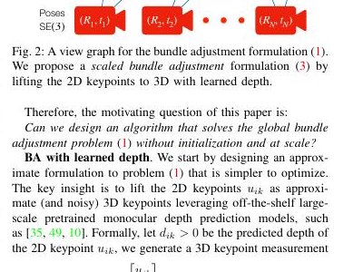
Fig. 2: A view graph for the bundle adjustment formulation (1). We propose a scaled bundle adjustment formulation (3) by lifting the 2D keypoints to 3D with learned depth.
图 2:束调整公式 (1) 的视角图。我们提出缩放束调整公式 (3),用学习深度把二维关键点提升到三维。
BA with learned depth. We start by designing an approximate formulation to problem (1) that is simpler to optimize. The key insight is to lift the 2D keypoints as approximate (and noisy) 3D keypoints leveraging off-the-shelf large-scale pretrained monocular depth prediction models, such as [35, 49, 10]. Formally, let be the predicted depth of the 2D keypoint , we generate a 3D keypoint measurement
带学习深度的 BA。我们先为问题 (1) 设计更易优化的近似公式。关键洞察是:借助现成大规模预训练单目深度预测模型(如 [35, 49, 10]),把二维关键点 提升为近似(且有噪声)的三维关键点。形式化地,令 为二维关键点 的预测深度,我们生成三维关键点测量
$$\displaystyle\tilde{\mathchar 29045}{\mathchar 29033\mathchar 29035}\mathchar 12349\mathchar 29028{\mathchar 29033\mathchar 29035}\begin{\mathchar29026\mathchar29037\mathchar29025\mathchar29044\mathchar29042\mathchar29033\mathchar29048}\mathchar 29045_{\mathchar 29033\mathchar 29035}\
\mathchar 28721\end{\mathchar29026\mathchar29037\mathchar29025\mathchar29044\mathchar29042\mathchar29033\mathchar29048}\mathchar 24891\quad\mathchar 568\delimiter 67273472\mathchar 29033\mathchar 24891\mathchar 29035\delimiter 84054785\mathchar 12850{\cal\mathchar 28997}\mathchar 314 \tag{2}$$
In our work, we select a metric depth model, which is designed to produce depth estimates that match the true depth when the model is perfectly trained. Further, due to imperfect depth prediction caused by potentially out-of-distribution test images, we incorporate a scaling parameter that allows subsequent optimization to correct erroneous predictions, leading to the following scaled bundle adjustment (SBA) formulation
在本文中,我们选用度量深度模型:在完美训练时,其深度估计与真值深度一致。进一步,由于测试图像可能分布外导致深度预测不完美,我们引入缩放参数,使后续优化能纠正错误预测,从而得到如下缩放束调整(SBA)公式
$$\displaystyle\min_{\begin{\mathchar29043\mathchar29045\mathchar29026\mathchar29025\mathchar29042\mathchar29042\mathchar29025\mathchar29049}{\mathchar29027}\mathchar 29040_{\mathchar 29035}\mathchar 12850{{\mathbb{\mathchar 29010}}^{\mathchar 28723}}\mathchar 24891\mathchar 29035\mathchar 12349\mathchar 28721\mathchar 24891\dots\mathchar 24891\mathchar 29005\
\mathchar 29043_{\mathchar 29033}\mathchar 12606\mathchar 28720\mathchar 24891\mathchar 29033\mathchar 12349\mathchar 28721\mathchar 24891\dots\mathchar 24891\mathchar 29006\
\delimiter 67273472\mathchar 29010_{\mathchar 29033}\mathchar 24891\mathchar 29044_{\mathchar 29033}\delimiter 84054785\mathchar 12850\mathrm{\mathchar 29011\mathchar 28997}\delimiter 67273472\mathchar 28723\delimiter 84054785\mathchar 24891\mathchar 29033\mathchar 12349\mathchar 28721\mathchar 24891\dots\mathchar 24891\mathchar 29006\end{\mathchar29043\mathchar29045\mathchar29026\mathchar29025\mathchar29042\mathchar29042\mathchar29025\mathchar29049}}\mathchar 4944\displaylimits_{\delimiter 67273472\mathchar 29033\mathchar 24891\mathchar 29035\delimiter 84054785\mathchar 12850{\cal\mathchar 28997}}\mathchar 29047_{\mathchar 29033\mathchar 29035}\left\delimiter 0\mathchar 29010_{\mathchar 29033}\delimiter 67273472\mathchar 29043_{\mathchar 29033}\tilde{\mathchar 29045}{\mathchar 29033\mathchar 29035}\delimiter 84054785\mathchar 8235\mathchar 29044{\mathchar 29033}\mathchar 8704\mathchar 29040_{\mathchar 29035}\right\delimiter 0^{\mathchar 28722}\mathchar 24891 \tag{3}$$
where scales the predicted 3D keypoint in (2), transforms the scaled 3D keypoint to the global frame,[^2] and the squared errors in the objective computes 3D distances to the landmarks without the reprojection . In (3), we allow weighting the squared errors by confidence values () from the depth prediction model.
其中 缩放 (2) 中的预测三维关键点 , 把缩放后的三维关键点变换到全局坐标系,[^2]目标中的平方误差计算到路标 的三维距离,而不经重投影 。在 (3) 中,我们允许用深度预测模型给出的置信度()加权平方误差。
Remark 1(Connection to Other Perception Problems).
It is worth noting that (i) without the per-frame scaling, problem (3) recovers the multiple point cloud registration problem [15, 26]; (ii) when (two frames), problem (3) reduces to (scaled) point cloud registration [25, 48].
注 1(与其他感知问题的联系)。
值得注意:(i) 去掉逐帧缩放时,问题 (3) 退化为多点云配准问题 [15, 26];(ii) 当 (两帧)时,问题 (3) 化为(缩放)点云配准 [25, 48]。
Through depth prediction, we removed the reprojection function from (1) and resolved one challenge. However, nonconvexity and large scale remain in problem (3).
通过深度预测,我们从 (1) 中去掉了重投影函数 ,解决了其中一个挑战。然而问题 (3) 中非凸性与大规模仍然存在。
Contributions. First, we show the remaining nonconvexity in problem (3) is “benign”. Our strategy is to first rewrite (3) as a quadratically constrained quadratic program (QCQP), and then design a convex semidefinite program (SDP) relaxation, in the spirit of a growing family of SDP-enabled certifiable algorithms [47, 38, 52, 28, 6, 33, 44]. We show the SDP relaxation is empirically tight, i.e., globally optimal solutions of the nonconvex (3) can be computed from the convex SDP relaxation with optimality certificates. Second, we show the convex SDP relaxations can be solved at extreme scale and speed—faster and more scalable than even the best local solvers such as Ceres. The enabling technique is to exploit the low-rankness of (tight) SDP optimal solutions via Burer-Monteiro (BM) factorization [13] and solve the resulting Riemannian optimization using a trust-region algorithm [11]. For the first time, we implemented the trust-region Riemannian optimizer directly in C++/CUDA and show the GPU implementation is up to times faster than the state-of-the-art CPU-based Manopt package [12] and can solve extreme-scale problems beyond the reach of Manopt (e.g., camera frames, see Fig. 1). We name our GPU solver XM (conveX bundle adjustMent). Third, we build a full SfM pipeline with XM as the optimization engine and various techniques from prior work, such as feature matching from Colmap, view graph creation from Glomap, Ceres refinement (i.e., warmstart Ceres with XM’s solutions for solving (1)), and outlier-robust filtering and estimation schemes [4, 20, 31, 40]. We test XM-SfM across six popular datasets and demonstrate that XM-SfM compares favorably with existing SfM pipelines in terms of reconstruction quality while being significantly faster, more scalable, and initialization-free, thanks to convex optimization and GPU-based implementation.
贡献。首先,我们证明问题 (3) 中剩余的非凸性是「良性」的。策略是先把 (3) 改写为二次约束二次规划(QCQP),再设计凸半定规划(SDP)松弛,呼应日益增多的可证明 SDP 算法族 [47, 38, 52, 28, 6, 33, 44]。我们表明 SDP 松弛在经验上是紧的,亦即非凸 (3) 的全局最优解可从凸 SDP 松弛连同最优性证书一并算出。其次,我们证明凸 SDP 松弛可在极端规模与速度下求解——甚至比 Ceres 等最佳局部求解器更快、更可扩展。关键技术是借 Burer-Monteiro(BM)分解 [13] 利用(紧)SDP 最优解的低秩性,并用信赖域算法 [11] 求解所得黎曼优化。我们首次直接在 C++/CUDA 中实现信赖域黎曼优化器,并表明 GPU 实现相对当前最优的基于 CPU 的 Manopt 包 [12] 可快至 倍,并能求解 Manopt 力所不及的极端规模问题(例如 个相机帧,见图 1)。我们将 GPU 求解器命名为 XM(conveX bundle adjustMent)。第三,我们以 XM 为优化引擎,结合 Colmap 特征匹配、Glomap 视角图构建、Ceres 精修(即以 XM 解为 warmstart 求解 (1))以及抗野值滤波与估计方案 [4, 20, 31, 40] 等先前技术,构建完整 SfM 管线。我们在六个流行数据集上测试 XM-SfM,表明其在重建质量上可与现有 SfM 管线媲美,同时因凸优化与 GPU 实现而显著更快、更可扩展且无需初始化。
In summary, our contributions are:
总结起来,我们的贡献是:
- • designing an empirically tight convex SDP relaxation for the scaled bundle adjustment problem (3);
- • 为缩放束调整问题 (3) 设计经验上紧的凸 SDP 松弛;
- • solving the convex SDP at extreme scales using BM factorization paired with a trust-region Riemannian optimizer directly implemented in C++/CUDA, i.e., XM;
- • 用 BM 分解配合直接以 C++/CUDA 实现的信赖域黎曼优化器在极端规模上求解凸 SDP,即 XM;
- • creating a full SfM pipeline called XM-SfM that “builds Rome with convex optimization”.
- • 创建完整 SfM 管线 XM-SfM,「用凸优化建造罗马」。
Paper organization. We derive the QCQP formulation for (3) and design the SDP relaxation in §II. We present BM factorization and the CUDA-based trust-region Riemannian optimizer in §III. We describe the XM-SfM pipeline in §IV and present experimental results in §V. We conclude in §VI.
论文组织。§II 推导 (3) 的 QCQP 公式并设计 SDP 松弛。§III 给出 BM 分解与基于 CUDA 的信赖域黎曼优化器。§IV 描述 XM-SfM 管线,§V 给出实验结果。§VI 作结。
II QCQP and Convex SDP Relaxation
II QCQP 与凸 SDP 松弛
In this section, let us focus on solving the SBA problem (3) to certifiable global optimality. We proceed in two steps. In §II-A, we simplify the original formulation as a quadratically constrained quadratic program (QCQP) through a sequence of mathematical manipulations. In §II-B, we apply Shor’s semidefinite relaxation to “convexify” the nonconvex QCQP.
本节聚焦把 SBA 问题 (3) 求解到可证明的全局最优。分两步:§II-A 经一系列数学处理把原公式化简为二次约束二次规划(QCQP);§II-B 应用 Shor 半定松弛以「凸化」非凸 QCQP。
Before we get started, we remove the ambiguity of problem (3) through anchoring.
开始之前,我们通过锚定消除问题 (3) 的歧义。
Anchoring. Observe that one can choose , , and the objective value of (3) can be set arbitrarily close to zero. Additionally, multiplying an arbitary rotation matrix on does not change the objective of (3), leading to infinitely many solutions. To resolve these issues, we anchor the first frame and set .
锚定。观察到可选取 , ,并使 (3) 的目标值任意接近零。此外,对 乘任意旋转矩阵不改变 (3) 的目标,导致无穷多解。为消除这些问题,我们锚定第一帧并令 .
II-A QCQP Formulation
II-A QCQP 公式
We first show that the unconstrained variables in (3), namely the translations and the 3D landmarks , can be “marginalized out”, leading to an optimization problem only concerning the scaling factors and 3D rotations.
我们先证明 (3) 中的无约束变量,即平移 与三维路标 ,可被「边缘化掉」,从而得到只关乎缩放因子与三维旋转的优化问题。
Proposition 2(Scaled-Rotation-Only Formulation).
Problem(3)is equivalent to the following optimization
命题 2(仅缩放–旋转公式)。
问题 (3) 等价于如下优化
\displaystyle\mathchar 28954^{\mathchar 8511}\mathchar 12349\min \\ \displaystyle\ \ \mathrm{\mathchar 29044\mathchar 29042}\left\delimiter 67273472\mathchar 29009\mathchar 29013^{\mathsf{\mathchar 29012}}\mathchar 29013\right\delimiter 84054785 \\ \displaystyle\ \ \mathchar 29013\mathchar 12349\left\delimiter 67482370\begin{array}[]{cccc}{\mathbf{\mathchar 29001}}_{\mathchar 28723}&\mathchar 29043_{\mathchar 28722}\mathchar 29010_{\mathchar 28722}&\mathinner{\mathpunct{\mathchar 513}\mathpunct{\mathchar 513}\mathpunct{\mathchar 513}}&\mathchar 29043_{\mathchar 29006}\mathchar 29010_{\mathchar 29006}\end{array}\right\delimiter 84267779 \\ \displaystyle\ \ \mathchar 29043_{\mathchar 29033}\mathchar 12606\mathchar 28720\mathchar 24891\mathchar 29010_{\mathchar 29033}\mathchar 12850\mathrm{\mathchar 29011\mathchar 29007}\delimiter 67273472\mathchar 28723\delimiter 84054785\mathchar 24891\quad\mathchar 29033\mathchar 12349\mathchar 28722\mathchar 24891\mathinner{\mathpunct{\mathchar 513}\mathpunct{\mathchar 513}\mathpunct{\mathchar 513}}\mathchar 24891\mathchar 29006 \tag{4a}
where is a constant and symmetric “data matrix” whose expression is given in Appendix A-A.
其中 是常数对称「数据矩阵」,表达式见附录 A-A。
Let represent the optimal solution of(4)and let be the concatenation of translations, be the concatenation of landmark positions. The optimal translations and landmark positions of problem (3) can be recovered from as follows:
令 表示 (4) 的最优解,令 为平移的拼接, 为路标位置的拼接。问题 (3) 的最优平移 与路标位置 可由 如下恢复:
$$\displaystyle\left\delimiter 67482370\begin{array}[]{c}\mathchar 29044^{\mathchar 8511}\
\mathchar 29040^{\mathchar 8511}\end{array}\right\delimiter 84267779\mathchar 12349\delimiter 67273472\mathchar 28993\mathchar 8714{\mathbf{\mathchar 29001}}_{\mathchar 28723}\delimiter 84054785\mathrm{\delimiter 69640972\mathchar 29029\mathchar 29027}\left\delimiter 67273472\mathchar 29013^{\mathchar 8511}\right\delimiter 84054785\mathchar 314$$
where the expression of can be found in Appendix A-A.
其中 的表达式见附录 A-A。
Proof.
See Appendix A-A. ∎
证明。
见附录 A-A。∎
Proposition 2 reformulates the SBA problem (3) as a lower-dimensional problem (4). However, problem (4) is not a QCQP because the objective function is a degree-four polynomial in and . In the next step, we show that it is possible to combine the “scaled rotation” together as a new variable, effectively reducing the degree of the polynomial.
命题 2 把 SBA 问题 (3) 改写为低维问题 (4)。然而问题 (4) 不是 QCQP,因为目标是关于 与 的四次多项式。下一步我们证明可以把「缩放旋转」 合并为新变量,从而有效降低多项式次数。
Proposition 3(QCQP Formulation).
Define the set of scaled orthogonal group as
命题 3(QCQP 公式)。
定义缩放正交群集合为
The set can be described by quadratic constraints
集合 可由二次约束刻画
$$\begin{split}\bar{\mathchar 29010}\mathchar 12349\left\delimiter 67482370\begin{array}[]{ccc}\mathchar 29027_{\mathchar 28721}&\mathchar 29027_{\mathchar 28722}&\mathchar 29027_{\mathchar 28723}\end{array}\right\delimiter 84267779\mathchar 12850\mathfrak{\mathchar 29043}\mathrm{\mathchar 29007}\delimiter 67273472\mathchar 28723\delimiter 84054785\mathrel{\mathchar 552\mkern-3.0mu\mathchar 553}\
\begin{cases}\mathchar 29027_{\mathchar 28721}^{\mathsf{\mathchar 29012}}\mathchar 29027_{\mathchar 28721}\mathchar 12349\mathchar 29027_{\mathchar 28722}^{\mathsf{\mathchar 29012}}\mathchar 29027_{\mathchar 28722}\mathchar 12349\mathchar 29027_{\mathchar 28723}^{\mathsf{\mathchar 29012}}\mathchar 29027_{\mathchar 28723}\
\mathchar 29027_{\mathchar 28721}^{\mathsf{\mathchar 29012}}\mathchar 29027_{\mathchar 28722}\mathchar 12349\mathchar 29027_{\mathchar 28722}^{\mathsf{\mathchar 29012}}\mathchar 29027_{\mathchar 28723}\mathchar 12349\mathchar 29027_{\mathchar 28723}^{\mathsf{\mathchar 29012}}\mathchar 29027_{\mathchar 28721}\mathchar 12349\mathchar 28720\mathchar 314\end{cases}\end{split} \tag{9}$$
Consider the following QCQP
考虑如下 QCQP
\displaystyle\mathchar 28954_{{\sf\mathchar 29009\mathchar 28995\mathchar 29009\mathchar 29008}}^{\mathchar 8511}\mathchar 12349\min \\ \displaystyle\ \ \mathrm{\mathchar 29044\mathchar 29042}\left\delimiter 67273472\mathchar 29009\mathchar 29013^{\mathsf{\mathchar 29012}}\mathchar 29013\right\delimiter 84054785 \\ \displaystyle\ \ \mathchar 29013\mathchar 12349\left\delimiter 67482370\begin{array}[]{cccc}{\mathbf{\mathchar 29001}}_{\mathchar 28723}&\bar{\mathchar 29010}_{\mathchar 28722}&\mathinner{\mathpunct{\mathchar 513}\mathpunct{\mathchar 513}\mathpunct{\mathchar 513}}&\bar{\mathchar 29010}_{\mathchar 29006}\end{array}\right\delimiter 84267779 \\ \displaystyle\ \ \bar{\mathchar 29010}_{\mathchar 29033}\mathchar 12850\mathfrak{\mathchar 29043}\mathrm{\mathchar 29007}\delimiter 67273472\mathchar 28723\delimiter 84054785\mathchar 24891~\mathchar 29033\mathchar 12349\mathchar 28722\mathchar 24891\dots\mathchar 24891\mathchar 29006\mathchar 314 \tag{10a}
and let be a global optimizer. If
并令 为全局最优解。若
then is a global minimizer to problem(4).
则 是问题 (4) 的全局极小点。
Proof.
See Appendix A-B. ∎
证明。
见附录 A-B。∎
It is clear that
显然有
because from (4) to (10) we have relaxed the constraint to . After solving (10), if there exists some index such that , we can extract a feasible solution to (4) by projecting onto after extracting the scaling from .
因为从 (4) 到 (10) 我们把 约束松弛为 。求解 (10) 后,若存在某个指标 使得 ,则可先从 提取缩放,再投影到 ,从而得到 (4) 的可行解。
Remark 4(Bad Local Minimum).
Problem (10) is a nonconvex QCQP. In fact, it is a smooth Riemannian optimization by identifying as a product manifold of the positive manifold and the orthogonal group. Therefore, one can directly use, e.g., Manopt to solve (10) (and also (4)). However, as we will show in §V on the Mip-Nerf 360 dataset [7], directly solving (10) can get stuck in bad local minima.
注 4(坏局部极小)。
问题 (10) 是非凸 QCQP。实际上,通过把 视为正流形与正交群的乘积流形,它是光滑黎曼优化。因此可直接用 Manopt 等求解 (10)(以及 (4))。但如我们将在 §V 于 Mip-Nerf 360 数据集 [7] 上所示,直接求解 (10) 可能陷入坏局部极小。
This motivates and necessitates convex relaxation.
这促使并使得凸松弛成为必要。
II-B Convex SDP Relaxation
II-B 凸 SDP 松弛
For any QCQP, there exists a convex relaxation known as Shor’s semidefinite relaxation [46, Chapter 3]. The basic idea is fairly simple: by creating a matrix variable that is quadratic in the original variable , problem (10) becomes linear in . The convex relaxation proceeds by using convex positive semidefinite constraints and linear constraints to properly enforce the matrix variable .
对任意 QCQP,存在称为 Shor 半定松弛的凸松弛 [46, 第 3 章]。基本想法很简单:构造相对原变量 二次的矩阵变量 ,则问题 (10) 对 变为线性。凸松弛再用凸正半定约束与线性约束恰当强制矩阵变量 。
Proposition 5(SDP Relaxation).
The following semidefinite program (SDP)
命题 5(SDP 松弛)。
如下半定规划(SDP)
$$\displaystyle\mathchar 28954^{\mathchar 8511}{{\sf\mathchar 29011\mathchar 28996\mathchar 29008}}\mathchar 12349\min{\mathchar 29016\mathchar 12850\mathbb{\mathchar 29011}^{\mathchar 28723\mathchar 29006}} \ \displaystyle\ \ \mathrm{\mathchar 29044\mathchar 29042}\left\delimiter 67273472\mathchar 29009\mathchar 29016\right\delimiter 84054785 \ \displaystyle\ \ \mathchar 29016\mathchar 12349\left\delimiter 67482370\begin{array}[]{ccc}{\mathbf{\mathchar 29001}}{\mathchar 28723}&\mathinner{\mathpunct{\mathchar 513}\mathpunct{\mathchar 513}\mathpunct{\mathchar 513}}&\mathchar 8707\
\mathord{\vbox{\kern 6.0pt\hbox{.}\hbox{.}\hbox{.}}}&\mathinner{\mkern 1.0mu\raise 7.0pt\vbox{\kern 7.0pt\hbox{.}}\mkern 2.0mu\raise 4.0pt\hbox{.}\mkern 2.0mu\raise 1.0pt\hbox{.}\mkern 1.0mu}&\mathord{\vbox{\kern 6.0pt\hbox{.}\hbox{.}\hbox{.}}}\
&\mathinner{\mathpunct{\mathchar 513}\mathpunct{\mathchar 513}\mathpunct{\mathchar 513}}&\mathchar 28939{\mathchar 29006}{\mathbf{\mathchar 29001}}_{\mathchar 28723}\end{array}\right\delimiter 84267779\mathchar 12823\mathchar 28720 \tag{13a}$$
is a convex relaxation to(10), i.e.,
是对 (10) 的凸松弛,即
Let be a global minimizer of(13).
令 为 (13) 的全局极小点。
If \mathrm{\mathchar 29042\mathchar 29025\mathchar 29038\mathchar 29035}\left\delimiter 67273472\mathchar 29016^{\mathchar 8511}\right\delimiter 84054785\mathchar 12349\mathchar 28723, then can be factorized as , and it holds[^3]
若 \mathrm{\mathchar 29042\mathchar 29025\mathchar 29038\mathchar 29035}\left\delimiter 67273472\mathchar 29016^{\mathchar 8511}\right\delimiter 84054785\mathchar 12349\mathchar 28723,则 可分解为 ,并且有[^3]
\displaystyle\bar{\mathchar 29013}^{\mathchar 8511}\mathchar 12349\left\delimiter 67482370\begin{array}[]{cccc}\bar{\mathchar 29010}_{\mathchar 28721}^{\mathchar 8511}&\bar{\mathchar 29010}_{\mathchar 28722}^{\mathchar 8511}&\mathinner{\mathpunct{\mathchar 513}\mathpunct{\mathchar 513}\mathpunct{\mathchar 513}}&\bar{\mathchar 29010}_{\mathchar 29006}^{\mathchar 8511}\end{array}\right\delimiter 84267779\mathchar 12850\mathchar 29007\delimiter 67273472\mathchar 28723\delimiter 84054785\mathchar 8706\mathfrak{\mathchar 29043}\mathrm{\mathchar 29007}\delimiter 67273472\mathchar 28723\delimiter 84054785^{\mathchar 29006\mathchar 8704\mathchar 28721}\mathchar 314
Define
定义
then is a global optimizer to(10). In this case, we say the relaxation is tight or exact.
则 是 (10) 的全局最优解。此时称松弛是紧的或精确的。
Proof.
See Appendix A-C. ∎
证明。
见附录 A-C。∎
If \mathrm{\mathchar 29042\mathchar 29025\mathchar 29038\mathchar 29035}\left\delimiter 67273472\mathchar 29016^{\mathchar 8511}\right\delimiter 84054785\mathchar 12606\mathchar 28723, then we can extract feasible solutions to (10) by taking the top three eigenvectors of and project the corresponding entries to and further to scaled rotations, a step that is typically called rounding. Denote as the rounded solution that is feasible for (4), we can evaluate the objective of (4) at and denote it . Combining the chain of inequalities from (12) and (14), we get
若 \mathrm{\mathchar 29042\mathchar 29025\mathchar 29038\mathchar 29035}\left\delimiter 67273472\mathchar 29016^{\mathchar 8511}\right\delimiter 84054785\mathchar 12606\mathchar 28723,则可取 的前三个特征向量,并把对应条目投影到 ,再进一步投影到缩放旋转,这一步通常称为取整。记 为对 (4) 可行的取整解,在 处计算 (4) 的目标并记为 。合并 (12) 与 (14) 的不等式链,得
where the last inequality follows from is a feasible solution for the minimization problem (4). Assuming we can solve the convex SDP, we compute and at both ends of the inequality (18), allowing us to evaluate a relative suboptimality:
其中最后一个不等式源于 是极小化问题 (4) 的可行解。假定能求解凸 SDP,我们在不等式 (18) 两端计算 与 ,从而可评估相对次优性:
certifies global optimality of the rounded solution , and tightness of the SDP relaxation.
证明取整解 的全局最优性,以及 SDP 松弛的紧性。
Remark 6(Connection to Prior Work).
For readers familiar with SDP relaxations, this section should not be surprising at all—that is the reason why we kept this section very brief and only focus on milestone results listed in the propositions. The closest two works to ours areSE-Sync*[38] andSIM-Sync[52], and the SDP relaxation technique traces back to at least the work by Carlone et al. [14]. The novelty of our formulation are twofold: (a) we estimate scaling factors with the motivation to correct learned depth whileSE-Syncestimates rotations and translations only; (b) we jointly estimate 3D landmarks and (scaled) camera poses whileSIM-Syncdoes not estimate 3D landmarks. These differences allow us to solve the long-standing bundle adjustment problem with convex optimization.*
注 6(与先前工作的联系)。
对熟悉 SDP 松弛的读者,本节并不意外——这也是我们写得很短、只聚焦命题中里程碑结果的原因。与我们最接近的两篇工作是 SE-Sync [38] 与 SIM-Sync [52],SDP 松弛技术至少可追溯到 Carlone 等人 [14]。我们公式的新意有两点:(a) 我们估计缩放因子以纠正学习深度,而 SE-Sync 只估计旋转与平移;(b) 我们联合估计三维路标与(缩放)相机位姿,而 SIM-Sync 不估计三维路标。这些差异使我们能用凸优化求解长期存在的束调整问题。
We shall focus on how to solve the convex SDP (13).
我们将聚焦如何求解凸 SDP (13)。
III Burer-Monteiro Factorization and CUDA-based Riemannian Optimizer
III Burer-Monteiro 分解与基于 CUDA 的黎曼优化器
Let us first write the SDP (13) in standard primal form:
先把 SDP (13) 写成标准原形式:
\displaystyle\min_{\mathchar 29016\mathchar 12850\mathbb{\mathchar 29011}^{\mathchar 28723\mathchar 29006}} \\ \displaystyle\ \ \mathrm{\mathchar 29044\mathchar 29042}\left\delimiter 67273472\mathchar 29009\mathchar 29016\right\delimiter 84054785 \\ \displaystyle\ \ \delimiter 69632778\mathchar 28993_{\mathchar 29033}\mathchar 24891\mathchar 29016\delimiter 86414091\mathchar 12349\mathchar 29026_{\mathchar 29033}\mathchar 24891\mathchar 29033\mathchar 12349\mathchar 28721\mathchar 24891\dots\mathchar 24891\mathchar 29037 \\ \displaystyle\ \ \mathchar 29016\mathchar 12823\mathchar 28720 \tag{20a}
where we have rewritten the constraint (13) as a positive semidefinite (PSD) constraint (20c) and linear equality constraints (20b). To see why this reformulation is true, note that the diagonal blocks of are either or scaled —the former can be enforced using 6 linear equalities and the latter can be enforced using 5, summing up to linear equalities. Associated with the primal standard SDP (20) is the following dual standard SDP:
其中我们把约束 (13) 改写为正半定(PSD)约束 (20c) 以及 个线性等式约束 (20b)。该改写成立是因为 的对角 块要么是 ,要么是缩放的 ——前者可用 6 个线性等式强制,后者用 5 个,合计 个线性等式。与原标准 SDP (20) 相伴的是如下对偶标准 SDP:
Since Slater’s condition holds ( is feasible for the primal (20)), we know strong duality holds between primal (20) and dual (21), i.e., their optimal values are equal to each other [46, 45].
由于 Slater 条件成立( 对原问题 (20) 可行),故原问题 (20) 与对偶 (21) 强对偶成立,即最优值相等 [46, 45]。
Scalability. Once the SDP (13) is formulated in standard forms, it can be solved by off-the-shelf SDP solvers such as MOSEK [5], provided that the SDP’s scale is not so large. Our SDP relaxation leads to a matrix variable with size . This means that when is in the order of hundreds, MOSEK can solve the SDP without any problem. However, when is in the order of thousands or tens of thousands, which is not uncommon in bundle adjustment problems, MOSEK will become very slow or even runs out of memory (e.g., MOSEK becomes unresponsive when ). Therefore, we decided to customize a solver for our SDP relaxation.
可扩展性。一旦 SDP (13) 写成标准形式,只要规模不太大,就可用 MOSEK [5] 等现成 SDP 求解器求解。我们的 SDP 松弛导致矩阵变量规模为 。这意味着当 为数百量级时,MOSEK 可顺利求解。但当 为数千乃至数万(在束调整中并不少见)时,MOSEK 会非常慢甚至内存耗尽(例如当 时 MOSEK 无响应)。因此我们决定为该 SDP 松弛定制求解器。
III-A Burer-Monteiro Factorization
III-A Burer-Monteiro 分解
The key structure we will leverage is, as stated in Proposition 5, the optimal solution has its rank equal to three when the SDP relaxation is tight. In other words, the effective dimension of can be instead of .
我们利用的关键结构是:如命题 5 所述,当 SDP 松弛紧时,最优解 的秩等于三。换言之, 的有效维数可以是 而非 。
To exploit the low-rank structure, we will leverage the famous Burer-Monteiro (BM) factorization [13].
为利用低秩结构,我们将借助著名的 Burer-Monteiro(BM)分解 [13]。
Proposition 7(BM Factorization).
For a fixed rank , the Burer-Monteiro factorization of(13)and (20) reads:
命题 7(BM 分解)。
对固定秩 ,(13) 与 (20) 的 Burer-Monteiro 分解为:
$$\displaystyle\mathchar 28954^{\mathchar 8511}{{\sf\mathchar 28994\mathchar 29005}\mathchar 24891\mathchar 29042}\mathchar 12349\min{\bar{\mathchar 29010}{\mathchar 29033}\mathchar 12850{{\mathbb{\mathchar 29010}}^{\mathchar 29042\mathchar 8706\mathchar 28723}}\mathchar 24891\mathchar 29033\mathchar 12349\mathchar 28721\mathchar 24891\dots\mathchar 24891\mathchar 29006} \ \displaystyle\ \ \mathrm{\mathchar 29044\mathchar 29042}\left\delimiter 67273472\mathchar 29009\mathchar 29013^{\mathsf{\mathchar 29012}}\mathchar 29013\right\delimiter 84054785 \ \displaystyle\ \ \mathchar 29013\mathchar 12349\left\delimiter 67482370\begin{array}[]{ccc}\bar{\mathchar 29010}{\mathchar 28721}&\dots&\bar{\mathchar 29010}{\mathchar 29006}\end{array}\right\delimiter 84267779 \ \displaystyle\ \ \bar{\mathchar 29010}{\mathchar 29033}^{\mathsf{\mathchar 29012}}\bar{\mathchar 29010}{\mathchar 29033}\mathchar 12349\begin{cases}{\mathbf{\mathchar 29001}}{\mathchar 28723}&\mathchar 29033\mathchar 12349\mathchar 28721\
\mathchar 28939_{\mathchar 29033}{\mathbf{\mathchar 29001}}_{\mathchar 28723}&\mathchar 29033\mathchar 12821\mathchar 28722\end{cases}\mathchar 314 \tag{22a}$$
A few comments are in order. First, by factorizing , holds by construction. Second, note that when , problem (22) is exactly the same as the original QCQP (10) (up to the difference in ), and thus is NOT convex. Third, as long as where is the minimum rank of all optimal solutions of the SDP (13), the nonconvex BM factorization has the same global minimum as the convex SDP (13) [46, 13]. Note that the factor is a matrix of size , i.e., a flat matrix as shown in Fig. 3 bottom right.
有几点评注。第一,通过分解 ,正半定 自然成立。第二,当 时,问题 (22) 与原 QCQP (10) 实质相同(仅 有差异),因而并非凸的。第三,只要 ( 为 SDP (13) 所有最优解的最小秩),非凸 BM 分解与凸 SDP (13) 有相同的全局最小值 [46, 13]。注意因子 是规模为 的扁平矩阵,如图 3 右下所示。
Counterintuitive? The reader might find this confusing. In §II, we applied a series of techniques to relax a nonconvex optimization problem into a convex SDP, enabling us to solve it to global optimality. Surprisingly, the BM factorization appears to “undo” this effort, pulling us back into nonconvex optimization. While the low-rank factorization offers a clear scalability advantage, it remains uncertain whether this benefit outweighs the drawbacks of reintroducing nonconvexity.
反直觉? 读者或许困惑:§II 中我们用一系列技术把非凸问题松弛成凸 SDP,以便求到全局最优;BM 分解却似乎「撤销」了这些努力,把我们拉回非凸优化。虽然低秩分解有明确的可扩展优势,但这是否足以抵消重新引入非凸性的代价,仍不显然。
Rank “staircase”. The secret ingredient of BM factorization to tackle nonconvexity is that we will solve the factorized problem (22) at increasing ranks, like stepping up a “staircase” (cf. Fig. 3 bottom right). We will start with the lowest rank and solve problem (22) using local optimization. One of two cases will happen. (a) The local optimizer is the same as the global optimizer of the SDP, in which case we can leverage the dual SDP (21) to certify global optimality and declare victory against the SDP. (b) The local optimizer is not the same as the global optimizer of the SDP, in which case we can again leverage the dual SDP (21) to “escape” the bad local minimum via increasing the rank, i.e., going up the staircase.
秩「阶梯」。BM 分解对付非凸性的秘诀是:我们按递增的秩求解分解问题 (22),如同登上「阶梯」(参见图 3 右下)。从最低秩 出发,用局部优化求解 (22)。将出现两种情形之一。(a) 局部最优与 SDP 全局最优相同,则可借助对偶 SDP (21) 证明全局最优,宣告相对 SDP 获胜。(b) 局部最优不是 SDP 全局最优,则同样可借助对偶 SDP (21),通过升秩(登上阶梯)「逃离」坏局部极小。
We formalize this in Algorithm 1 and prove its correctness.
我们把这形式化为算法 1 并证明其正确性。
1: Input: the data matrix 2: Output: optimal solution 3: # Initialization 4: Set , 5: while True do 6: # Local optimization of (22) 7: 8: # Compute dual certificate 9: 1 10: # Certify global optimality 2 11: if then 12: return 13: # Escape local minimum 14: 15: \mathchar 29013_{\mathchar 29042\mathchar 8235\mathchar 28721}\mathchar 12349\left\delimiter 67482370\begin{array}[]{cc}\mathchar 29013_{\mathchar 29042}^{\mathsf{\mathchar 29012}}&\mathchar 28939\delimiter 69640972\end{array}\right\delimiter 84267779^{\mathsf{\mathchar 29012}} with 16: # Line search 17: while \mathrm{\mathchar 29044\mathchar 29042}\left\delimiter 67273472\mathchar 29009\mathchar 29013_{\mathchar 29042\mathchar 8235\mathchar 28721}\mathchar 29013_{\mathchar 29042\mathchar 8235\mathchar 28721}^{\mathsf{\mathchar 29012}}\right\delimiter 84054785\mathchar 12821\mathrm{\mathchar 29044\mathchar 29042}\left\delimiter 67273472\mathchar 29009\mathchar 29013_{\mathchar 29042}\mathchar 29013_{\mathchar 29042}^{\mathsf{\mathchar 29012}}\right\delimiter 84054785 do 18: 19: \mathchar 29013_{\mathchar 29042\mathchar 8235\mathchar 28721}\mathchar 12349\left\delimiter 67482370\begin{array}[]{cc}\mathchar 29013_{\mathchar 29042}^{\mathsf{\mathchar 29012}}&\mathchar 28939\delimiter 69640972\end{array}\right\delimiter 84267779^{\mathsf{\mathchar 29012}} 20: ,
1: Input: the data matrix
2: Output: optimal solution
3: # Initialization
4: Set ,
5: while True do
6: # Local optimization of (22)
7:
8: # Compute dual certificate
9: 1
10: # Certify global optimality 2
11: if then
12: return
13: # Escape local minimum
14:
15: \mathchar 29013_{\mathchar 29042\mathchar 8235\mathchar 28721}\mathchar 12349\left\delimiter 67482370\begin{array}[]{cc}\mathchar 29013_{\mathchar 29042}^{\mathsf{\mathchar 29012}}&\mathchar 28939\delimiter 69640972\end{array}\right\delimiter 84267779^{\mathsf{\mathchar 29012}} with
16: # Line search
17: while \mathrm{\mathchar 29044\mathchar 29042}\left\delimiter 67273472\mathchar 29009\mathchar 29013_{\mathchar 29042\mathchar 8235\mathchar 28721}\mathchar 29013_{\mathchar 29042\mathchar 8235\mathchar 28721}^{\mathsf{\mathchar 29012}}\right\delimiter 84054785\mathchar 12821\mathrm{\mathchar 29044\mathchar 29042}\left\delimiter 67273472\mathchar 29009\mathchar 29013_{\mathchar 29042}\mathchar 29013_{\mathchar 29042}^{\mathsf{\mathchar 29012}}\right\delimiter 84054785 do
18:
19: \mathchar 29013_{\mathchar 29042\mathchar 8235\mathchar 28721}\mathchar 12349\left\delimiter 67482370\begin{array}[]{cc}\mathchar 29013_{\mathchar 29042}^{\mathsf{\mathchar 29012}}&\mathchar 28939\delimiter 69640972\end{array}\right\delimiter 84267779^{\mathsf{\mathchar 29012}}
20: ,
1: Input: the data matrix
2: Output: optimal solution
3: # Initialization
4: Set ,
5: while True do
6: # Local optimization of (22)
7:
8: # Compute dual certificate
9: 1
10: # Certify global optimality 2
11: if then
12: return
13: # Escape local minimum
14:
15: \mathchar 29013_{\mathchar 29042\mathchar 8235\mathchar 28721}\mathchar 12349\left\delimiter 67482370\begin{array}[]{cc}\mathchar 29013_{\mathchar 29042}^{\mathsf{\mathchar 29012}}&\mathchar 28939\delimiter 69640972\end{array}\right\delimiter 84267779^{\mathsf{\mathchar 29012}} with
16: # Line search
17: while \mathrm{\mathchar 29044\mathchar 29042}\left\delimiter 67273472\mathchar 29009\mathchar 29013_{\mathchar 29042\mathchar 8235\mathchar 28721}\mathchar 29013_{\mathchar 29042\mathchar 8235\mathchar 28721}^{\mathsf{\mathchar 29012}}\right\delimiter 84054785\mathchar 12821\mathrm{\mathchar 29044\mathchar 29042}\left\delimiter 67273472\mathchar 29009\mathchar 29013_{\mathchar 29042}\mathchar 29013_{\mathchar 29042}^{\mathsf{\mathchar 29012}}\right\delimiter 84054785 do
18:
19: \mathchar 29013_{\mathchar 29042\mathchar 8235\mathchar 28721}\mathchar 12349\left\delimiter 67482370\begin{array}[]{cc}\mathchar 29013_{\mathchar 29042}^{\mathsf{\mathchar 29012}}&\mathchar 28939\delimiter 69640972\end{array}\right\delimiter 84267779^{\mathsf{\mathchar 29012}}
20: ,
Algorithm 1 Riemannian Staircase
1: 输入: 数据矩阵 2: 输出: 最优解 3: # Initialization 4: Set , 5: while True do 6: # Local optimization of (22) 7: 8: # 计算 对偶 证书 9: 1 10: # Certify global optimality 2 11: if then 12: 返回 13: # Escape 局部 minimum 14: 15: \mathchar 29013_{\mathchar 29042\mathchar 8235\mathchar 28721}\mathchar 12349\left\delimiter 67482370\begin{array}[]{cc}\mathchar 29013_{\mathchar 29042}^{\mathsf{\mathchar 29012}}&\mathchar 28939\delimiter 69640972\end{array}\right\delimiter 84267779^{\mathsf{\mathchar 29012}} with 16: # Line search 17: while \mathrm{\mathchar 29044\mathchar 29042}\left\delimiter 67273472\mathchar 29009\mathchar 29013_{\mathchar 29042\mathchar 8235\mathchar 28721}\mathchar 29013_{\mathchar 29042\mathchar 8235\mathchar 28721}^{\mathsf{\mathchar 29012}}\right\delimiter 84054785\mathchar 12821\mathrm{\mathchar 29044\mathchar 29042}\left\delimiter 67273472\mathchar 29009\mathchar 29013_{\mathchar 29042}\mathchar 29013_{\mathchar 29042}^{\mathsf{\mathchar 29012}}\right\delimiter 84054785 do 18: 19: \mathchar 29013_{\mathchar 29042\mathchar 8235\mathchar 28721}\mathchar 12349\left\delimiter 67482370\begin{array}[]{cc}\mathchar 29013_{\mathchar 29042}^{\mathsf{\mathchar 29012}}&\mathchar 28939\delimiter 69640972\end{array}\right\delimiter 84267779^{\mathsf{\mathchar 29012}} 20: ,
1: 输入: 数据矩阵
2: 输出: 最优解
3: # Initialization
4: Set ,
5: while True do
6: # Local optimization of (22)
7:
8: # 计算 对偶 证书
9: 1
10: # Certify global optimality 2
11: if then
12: 返回
13: # Escape 局部 minimum
14:
15: \mathchar 29013_{\mathchar 29042\mathchar 8235\mathchar 28721}\mathchar 12349\left\delimiter 67482370\begin{array}[]{cc}\mathchar 29013_{\mathchar 29042}^{\mathsf{\mathchar 29012}}&\mathchar 28939\delimiter 69640972\end{array}\right\delimiter 84267779^{\mathsf{\mathchar 29012}} with
16: # Line search
17: while \mathrm{\mathchar 29044\mathchar 29042}\left\delimiter 67273472\mathchar 29009\mathchar 29013_{\mathchar 29042\mathchar 8235\mathchar 28721}\mathchar 29013_{\mathchar 29042\mathchar 8235\mathchar 28721}^{\mathsf{\mathchar 29012}}\right\delimiter 84054785\mathchar 12821\mathrm{\mathchar 29044\mathchar 29042}\left\delimiter 67273472\mathchar 29009\mathchar 29013_{\mathchar 29042}\mathchar 29013_{\mathchar 29042}^{\mathsf{\mathchar 29012}}\right\delimiter 84054785 do
18:
19: \mathchar 29013_{\mathchar 29042\mathchar 8235\mathchar 28721}\mathchar 12349\left\delimiter 67482370\begin{array}[]{cc}\mathchar 29013_{\mathchar 29042}^{\mathsf{\mathchar 29012}}&\mathchar 28939\delimiter 69640972\end{array}\right\delimiter 84267779^{\mathsf{\mathchar 29012}}
20: ,
1: 输入: 数据矩阵
2: 输出: 最优解
3: # Initialization
4: Set ,
5: while True do
6: # Local optimization of (22)
7:
8: # 计算 对偶 证书
9: 1
10: # Certify global optimality 2
11: if then
12: 返回
13: # Escape 局部 minimum
14:
15: \mathchar 29013_{\mathchar 29042\mathchar 8235\mathchar 28721}\mathchar 12349\left\delimiter 67482370\begin{array}[]{cc}\mathchar 29013_{\mathchar 29042}^{\mathsf{\mathchar 29012}}&\mathchar 28939\delimiter 69640972\end{array}\right\delimiter 84267779^{\mathsf{\mathchar 29012}} with
16: # Line search
17: while \mathrm{\mathchar 29044\mathchar 29042}\left\delimiter 67273472\mathchar 29009\mathchar 29013_{\mathchar 29042\mathchar 8235\mathchar 28721}\mathchar 29013_{\mathchar 29042\mathchar 8235\mathchar 28721}^{\mathsf{\mathchar 29012}}\right\delimiter 84054785\mathchar 12821\mathrm{\mathchar 29044\mathchar 29042}\left\delimiter 67273472\mathchar 29009\mathchar 29013_{\mathchar 29042}\mathchar 29013_{\mathchar 29042}^{\mathsf{\mathchar 29012}}\right\delimiter 84054785 do
18:
19: \mathchar 29013_{\mathchar 29042\mathchar 8235\mathchar 28721}\mathchar 12349\left\delimiter 67482370\begin{array}[]{cc}\mathchar 29013_{\mathchar 29042}^{\mathsf{\mathchar 29012}}&\mathchar 28939\delimiter 69640972\end{array}\right\delimiter 84267779^{\mathsf{\mathchar 29012}}
20: ,
Algorithm 1 Riemannian Staircase
Certify global optimality. At every iteration of Algorithm 1, it first computes a local optimizer of the BM factorization problem (22) in line 7 using an algorithm to be described in §III-B. Denote the local optimizer as . To check whether is the optimal solution to the convex SDP (13), we need to compute the dual optimality certificate.
证明全局最优。在算法 1 的每次迭代中,先在第 7 行用 §III-B 所述算法计算 BM 分解问题 (22) 的局部最优解,记为 。要检查 是否为凸 SDP (13) 的最优解,需计算对偶最优性证书。
Theorem 8(Dual Optimality Certificate).
Let be a locally optimal solution of(22). Then, the linear independence constraint qualification (LICQ) must hold at , i.e.,
定理 8(对偶最优性证书)。
令 为 (22) 的局部最优解。则在 处线性无关约束规格(LICQ)必成立,即
are linearly independent. Hence, there must exist a unique dual variable such that
线性无关。因此必存在唯一对偶变量 使得
If further,
若进一步,
then is a global optimizer of(22), and , are optimal for the SDP(20)and its dual(21).
则 是 (22) 的全局最优解,且 、、 分别对 SDP (20) 及其对偶 (21) 最优。
Proof.
In general, LICQ may not hold at a locally optimal solution of the BM factorization. However, in Appendix A-D, we show that the unique structure of our XM SDP relaxation leads to guaranteed satisfaction of LICQ. The rest of the Theorem is standard and follows from [13] or [46]. ∎
证明。
一般情形下,LICQ 未必在 BM 分解的局部最优处成立。但在附录 A-D 中,我们证明 XM SDP 松弛的独特结构保证 LICQ 成立。定理其余部分是标准的,见 [13] 或 [46]。∎
Theorem 8 provides a simple recipe to certify global optimality by solving the linear system of equations in (24) (recall is linear in from (21b)), forming the dual matrix , and checking its positive semidefinite-ness.
定理 8 给出证明全局最优的简单配方:求解 (24) 中的线性方程组(回顾由 (21b), 对 线性),构造对偶矩阵 ,并检查其正半定性。
Escape local minimum. If is not PSD, then is not optimal for the SDP. In this case, the following theorem states that the eigenvector of corresponding to the minimum eigenvalue provides a descent direction.
逃离局部极小。若 不是正半定,则 对 SDP 非最优。此时下列定理指出:对偶矩阵最小特征值对应的特征向量给出下降方向。
Theorem 9(Descent Direction).
Let be a local minimizer of problem(22)and be the corresponding dual variable. Suppose is not PSD and is an eigenvector of corresponding to a negative eigenvalue. Then, consider the BM factorization(22)at rank . The direction
定理 9(下降方向)。
令 为问题 (22) 的局部极小点, 为对应对偶变量。设 非正半定,且 是其负特征值对应的特征向量。则考虑秩为 的 BM 分解 (22)。方向
$$\displaystyle\mathchar 28996\mathchar 12349\left\delimiter 67482370\begin{array}[]{c}\mathchar 28720\
\delimiter 69640972^{\mathchar 29012}\end{array}\right\delimiter 84267779$$
is a descent direction at the point
是该点处的下降方向
$$\displaystyle\hat{\mathchar 29013}\mathchar 12349\left\delimiter 67482370\begin{array}[]{c}\mathchar 29013^{\mathchar 8511}_{\mathchar 29042}\
\mathchar 28720\end{array}\right\delimiter 84267779\mathchar 314$$
Proof.
See [13] or [46]. ∎
证明。
见 [13] 或 [46]。∎
Theorem 9 states that if Algorithm 1 gets stuck at rank , it can escape the local minimum by increasing the rank. Since is a descent direction, we perform line search in lines 18-19 until a point with lower objective value is found.
定理 9 表明:若算法 1 在秩 卡住,可通过升秩逃离局部极小。由于 是下降方向,我们在第 18–19 行做线搜索,直到找到目标值更低的点。
Global convergence. Algorithm 1 is guaranteed to converge to the optimal solution of the SDP, as stated below.
全局收敛。算法 1 保证收敛到 SDP 的最优解,如下所述。
Theorem 10(Global Convergence).
Algorithm 1 finds a globally optimal solution of the SDP pair (20)-(21) regardless of the initialization point at .
定理 10(全局收敛)。
无论在 处的初始化点 如何,算法 1 都能找到 SDP 对 (20)–(21) 的全局最优解。
Proof.
We show that, in the worst case where , every local optimizer of the BM factorization (22) corresponds to a globally optimal solution of the SDP [27, Corollary 8]. To see this, if the locally optimal solution at is rank-deficient, then global optimality is guaranteed by the “rank deficiency” Lemma [13, Proposition 4]. Conversely, if the solution is full-rank, then must be zero—hence also positive semidefinite—as a result of solving (24), which again implies global optimality of the SDP. ∎
证明。
我们证明:在最坏情形 时,BM 分解 (22) 的每个局部最优都对应 SDP 的全局最优解 [27, 推论 8]。具体地,若 处的局部最优解亏秩,则由「亏秩」引理 [13, 命题 4] 保证全局最优;反之若满秩,则求解 (24) 的结果使 必为零——因而也正半定——再次蕴含 SDP 全局最优。∎
This property ensures that our approach is initialization-free. To verify the correctness of the theory, we conducted experiments on the BAL-93 dataset using random initializations, and after 1000 trials, our method achieved a 100% success rate.
该性质保证我们的方法无需初始化。为验证理论正确性,我们在 BAL-93 数据集上用随机初始化做实验,1000 次试验后成功率达 100%。
It is worth noting that, in the worst case when is increased to , the BM factorization does not have any scalability advantage over the original SDP. Fortunately, in almost all numerical experiments, Algorithm 1 terminates when or , bringing significant scalability advantage to solving large-scale SDP relaxations.
值得注意:在最坏情形当 增至 时,BM 分解相对原 SDP 并无可扩展优势。幸运的是,几乎所有数值实验中算法 1 在 或 时即终止,从而为大规模 SDP 松弛带来显著可扩展优势。
III-B C++/CUDA-based Riemannian Optimization
III-B 基于 C++/CUDA 的黎曼优化
Everything in Algorithm 1 is clear except line 7 where one needs to locally optimize the nonconvex BM factorization (22).
算法 1 中除第 7 行外都清楚:该行需对非凸 BM 分解 (22) 做局部优化。
Riemannian structure. At first glance, problem (22) looks like a nonconvex constrained optimization problem. However, the constraints of (22) indeed define a smooth manifold.
黎曼结构。乍看问题 (22) 像非凸约束优化。但其约束实际上定义了光滑流形。
Proposition 11(BM Riemannian Optimization).
The BM factorization problem (22) is equivalent to the following unconstrained Riemannian optimization problem
命题 11(BM 黎曼优化)。
BM 分解问题 (22) 等价于如下无约束黎曼优化问题
\displaystyle\min \\ \displaystyle\mathrm{\mathchar 29044\mathchar 29042}\left\delimiter 67273472\mathchar 29009\mathchar 29013^{\mathsf{\mathchar 29012}}\mathchar 29013\right\delimiter 84054785 \\ \displaystyle\mathchar 29013\mathchar 12349\left\delimiter 67482370\begin{array}[]{cccc}\mathchar 29010_{\mathchar 28721}&\mathchar 29043_{\mathchar 28722}\mathchar 29010_{\mathchar 28722}&\mathinner{\mathpunct{\mathchar 513}\mathpunct{\mathchar 513}\mathpunct{\mathchar 513}}&\mathchar 29043_{\mathchar 29006}\mathchar 29010_{\mathchar 29006}\end{array}\right\delimiter 84267779 \\ \displaystyle\mathchar 29043_{\mathchar 29033}\mathchar 12850\mathcal{\mathchar 29005}_{\mathchar 29040}\mathchar 24891\mathchar 29033\mathchar 12349\mathchar 28722\mathchar 24891\ldots\mathchar 24891\mathchar 29006\mathchar 24891 \\ \displaystyle\mathchar 29010_{\mathchar 29033}\mathchar 12850\mathcal{\mathchar 29005}_{\mathchar 29043}^{\delimiter 67273472\mathchar 29042\delimiter 84054785}\mathchar 24891\mathchar 29033\mathchar 12349\mathchar 28721\mathchar 24891\ldots\mathchar 24891\mathchar 29006 \tag{32a}
where is the positive manifold defined as
其中 是定义为如下的正流形
and is the Stiefel manifold of order :
而 是阶为 的 Stiefel 流形:
Proof.
By inspection. ∎
证明。
由观察即得。∎
We solve problem (32) using the Riemannian trust-region algorithm with truncated conjugate gradient (Rtr-tCG). Details of this algorithm can be found in [1, 11].
我们用带截断共轭梯度的黎曼信赖域算法(Rtr-tCG)求解问题 (32)。算法细节见 [1, 11]。
C++/CUDA implementation. The Rtr-tCG algorithm is readily available through the Manopt package [12]. However, to boost efficiency and enable fast solution of the SDP relaxation, we implement the Rtr-tCG algorithm directly in C++/CUDA, using analytical hessian-vector product.
C++/CUDA 实现。Rtr-tCG 算法可通过 Manopt 包 [12] 直接使用。但为提升效率、快速求解 SDP 松弛,我们直接在 C++/CUDA 中实现 Rtr-tCG,并使用解析 Hessian–向量积。
- • Conjugate gradient method. The conjugate gradient method involves only Hessian-vector products and vector addition. The Hessian-vector product can be decomposed into two components: (a) the Euclidean Hessian-vector product and (b) the Riemannian projection onto the tangent space. The first component primarily requires matrix-vector multiplication, which can be efficiently implemented using cuBLAS. The second component involves batched small matrix-matrix multiplications, matrix-matrix inner products, scalar-matrix multiplications, all of which are implemented using custom CUDA kernels. For vector addition, we directly utilize the cublasDaxpy function from cuBLAS.
- • 共轭梯度法。共轭梯度只涉及 Hessian–向量积与向量加法。Hessian–向量积可拆成:(a) 欧氏 Hessian–向量积;(b) 到切空间的黎曼投影。前者主要是矩阵–向量乘,可用 cuBLAS 高效实现;后者涉及批量小矩阵乘、矩阵内积、标量–矩阵乘,均用定制 CUDA 核实现。向量加法直接用 cuBLAS 的 cublasDaxpy。
- • Retraction. The retraction operation aims to map a point from the tangent space back to the manifold. In our case, the retraction operation happens both on the positive manifold and the Stiefel manifold. The retraction on the positive manifold is a simple custom kernel, while the retraction on the Stiefel manifold involves QR decomposition. We directly apply Gram-Schmidt process on every batch of matrices, which is implemented using custom CUDA kernels.
- • 回缩。回缩把切空间上的点映回流形。我们的情形下,回缩同时发生在正流形与 Stiefel 流形上。正流形上的回缩是简单定制核;Stiefel 上流形回缩涉及 QR 分解。我们对每批 矩阵直接做 Gram-Schmidt,并用定制 CUDA 核实现。
In §V, we show our GPU-based implementation achieves up to times speedup compared to the CPU-based Manopt.
在 §V 中我们表明:相对基于 CPU 的 Manopt,基于 GPU 的实现可快至 倍。
Remark 12(Connection to Prior Work).
This is not the first time BM factorization has been applied in robotics.SE-Syncand related works [18, 37] pioneered the application of BM factorization for solving the pose graph optimization problem. Several works [22, 21, 23, 24] utilized the dual optimality certificate result in Theorem 8 to develop fast certifiers. Our novelty lies in developing the first C++/CUDA-based implementation of the Riemannian trust-region algorithm to push the scalability limitations of BM factorization.
注 12(与先前工作的联系)。
这并非 BM 分解首次用于机器人。SE-Sync 及相关工作 [18, 37] 率先把 BM 分解用于位姿图优化。若干工作 [22, 21, 23, 24] 利用定理 8 的对偶最优性证书结果开发快速证明器。我们的新意在于给出首个基于 C++/CUDA 的黎曼信赖域算法实现,以突破 BM 分解的可扩展上限。
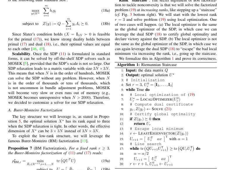
Fig. 3: XM-SfM: structure from motion pipeline with XM.
图 3:带 XM 的运动恢复结构管线 XM-SfM。
IV Structure from Motion with XM
IV 用 XM 做运动恢复结构
In this section, we present our SfM pipeline with XM as the optimization engine, illustrated in Fig. 3.
本节给出以 XM 为优化引擎的 SfM 管线,如图 3 所示。
View graph. To construct view graph for an image set, we first run Colmap’s feature extractor and exhaustive matcher to extract 2D correspondences. The feature extractor employs SIFT [30] for feature detection and description, while the exhaustive matcher matches every image pair. After matching, we apply Glomap’s track establishment to produce a four-column file where the first two columns represent feature point coordinates, the third indicates the image index, and the fourth corresponds to the 3D landmark indices. Currently, we use the original implementation from Colmap and Glomap. However, we remark that it is possible to speed up the processes further using C++ and GPU implementation. We leave this improvement for future work.
视角图。为图像集构建视角图时,我们先运行 Colmap 的特征提取器与穷尽匹配器得到二维对应。特征提取器用 SIFT [30] 做检测与描述,穷尽匹配器匹配每一图像对。匹配后应用 Glomap 的轨迹建立,生成四列表文件:前两列为特征点坐标,第三列为图像索引,第四列为三维路标索引。目前我们使用 Colmap 与 Glomap 的原始实现;亦可进一步用 C++ 与 GPU 加速,留作未来工作。
Depth estimation. We use the depth estimation model Unidepth [35] to calculate the metric depth of a given image, and lift the view graph from 2D to 3D. It is worth emphasizing that our test datasets do NOT belong to the training dataset of Unidepth. If given the confidence map, we use it to update the weight of different observations. We also tried other depth prediction models in Appendix B.
深度估计。我们用深度估计模型 Unidepth [35] 计算给定图像的度量深度,并把视角图从二维提升到三维。需要强调:我们的测试数据集不属于 Unidepth 的训练数据。若有置信度图,则用它更新不同观测的权重。附录 B 中我们也尝试了其他深度预测模型。
Filter from two-view estimation. Using 2D observations, we estimate the relative pose between two images. Based on this pose, we filter out 3D landmarks with large Euclidean distance errors. Specifically, landmarks with distance errors exceeding three times the median are removed.
来自两视图估计的滤波。利用二维观测估计两图像间相对位姿,据此滤除欧氏距离误差大的三维路标。具体地,距离误差超过中位数三倍的路标被移除。
XMsolver. We then use the lifted 3D measurements and the view-graph to form a matrix as shown in (4). We solve the SDP problem in (13) using our XM solver. If needed, we also delete the 10% measurements with the largest residuals and re-run the XM solver. This corresponds to a greedy heuristic for outlier removal [4, 40] and we call it XM2 (running twice).
XM 求解器。随后用提升后的三维测量与视角图按 (4) 构造 矩阵,并用 XM 求解器求解 SDP 问题 (13)。如有需要,再删除残差最大的 10% 测量并重新运行 XM。这对应野值剔除的贪心启发式 [4, 40],我们称之为 XM2(运行两次)。
Ceresrefinement. Usually the depth predictions are quite noisy, leading to inaccurate estimations of XM. We therefore also feed the estimated poses and landmarks to Ceres as a warmstart to solve the original bundle adjustment problem (1). As we will show, the solution of XM always provide a strong warmstart for Ceres to quickly optimize (1).
Ceres 精修。深度预测通常噪声较大,导致 XM 估计不够准。因此我们也把估计的位姿与路标作为热启动送入 Ceres,以求解原始束调整问题 (1)。后文将表明,XM 的解总能给 Ceres 提供强热启动,从而快速优化 (1)。
V Experiments
V 实验
Datasets BAL-93 (6033 landmarks) BAL-392 (13902 landmarks) BAL-1934 (67594 landmarks) BAL-10155 (33782 landmarks) Metrics Solver TimeProcessing Time ATE-TATE-R RPE-TRPE-R Solver TimeProcessing Time ATE-TATE-R RPE-TRPE-R Solver TimeProcessing Time ATE-TATE-R RPE-TRPE-R Solver TimeProcessing Time ATE-TATE-R RPE-TRPE-R Ceres Ceres-gt Ceres-gt-0.01 Ceres-gt-0.1 Manopt XM
TABLE I: Results on the BAL dataset. We report the ATE, RPE and running time for Ceres, Manopt, and our proposed XM solver. The evaluation is conducted on four BAL datasets with varying numbers of frames to demonstrate that our method is both fast and accurate across datasets of different scales (e.g., BAL-10155 indicates there are 10155 camera frames to be reconstructed). Ceres fails at a bad local minimum without a good initial guess, while Manopt performs significantly slower and even fails to solve within ten hours on the largest dataset.
数据集 BAL-93 (6033 路标) BAL-392 (13902 路标) BAL-1934 (67594 路标) BAL-10155 (33782 路标) 度量 Solver TimeProcessing Time ATE-TATE-R RPE-TRPE-R Solver TimeProcessing Time ATE-TATE-R RPE-TRPE-R Solver TimeProcessing Time ATE-TATE-R RPE-TRPE-R Solver TimeProcessing Time ATE-TATE-R RPE-TRPE-R Ceres Ceres-gt Ceres-gt-0.01 Ceres-gt-0.1 Manopt XM
表 I: 上的结果: BAL dataset. We report the ATE, RPE and running time for Ceres, Manopt, and our proposed XM solver. The evaluation is conducted on four BAL datasets with varying numbers of frames to demonstrate that our method is both fast and accurate across datasets of different scales (e.g., BAL-10155 indicates there are 10155 camera frames to be reconstructed). Ceres fails at a bad local minimum without a good initial guess, while Manopt performs significantly slower and even fails to solve within ten hours on the largest dataset.
Datasets BAL-93 BAL-392 BAL-1934 BAL-10155 Suboptimality-Gap Min-eig
TABLE II: Results on the BAL dataset (suboptimality and min-eig). We report the suboptimality gap and minimum eigenvalue of matrix in (21) for our proposed XM method.
数据集 BAL-93 BAL-392 BAL-1934 BAL-10155 次优间隙 最小特征值
表 II: 上的结果: BAL dataset (suboptimality and min-eig). We report the suboptimality gap and minimum eigenvalue of matrix in (21) for our proposed XM method.
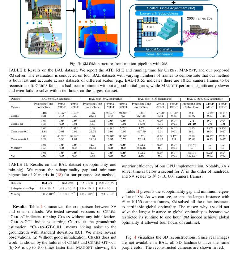
Fig. 4: Visualization of BAL datasets. Top: Our XM solver. Middle: Ceres-GT-0.01. Bottom: Ceres-GT-0.1. Both our XM solver and Ceres-GT-0.01 accurately recover the ground truth camera poses and landmarks, whereas Ceres-GT-0.1 fails.
图 4:BAL 数据集可视化。上: 我们的 XM 求解器。中: Ceres-GT-0.01。下: Ceres-GT-0.1。XM 与 Ceres-GT-0.01 均达到高精度。
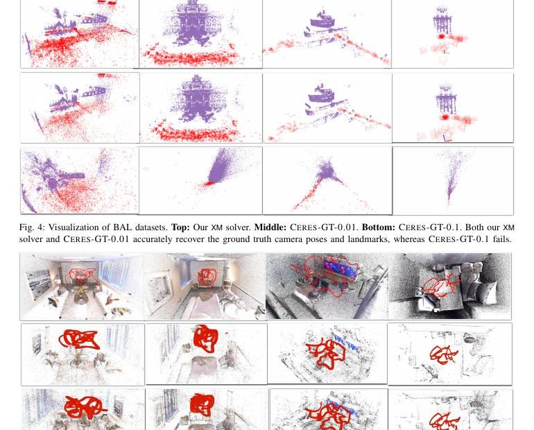
Fig. 5: Visualization of Replica datasets. Top: Our XM solver. Middle: Glomap. Bottom: Colmap. All methods achieve high accuracy, producing nearly identical reconstruction results. Glomap sometimes produce outliers (see column 2 and 3).
图 5:Replica 数据集可视化。上: 我们的 XM 求解器。中: Glomap。下: Colmap。各方法均达到高精度。
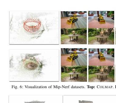
Fig. 6: Visualization of Mip-Nerf datasets. Top: Colmap. Bottom: Our XM solver. 3D-gaussian renderings are the same.
图 6:Mip-Nerf 数据集可视化。上: Colmap。下: 我们的 XM 求解器。三维高斯渲染结果相同。
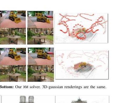
Fig. 7: Visualization of IMC2023 datasets. Top: Our XM solver. Bottom: Glomap.
图 7:IMC2023 数据集可视化。上: 我们的 XM 求解器。下: Glomap。
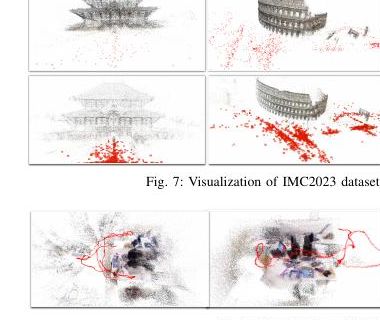
Fig. 8: Visualization of TUM datasets using our XM solver.
图 8:用我们的 XM 求解器可视化 TUM 数据集。
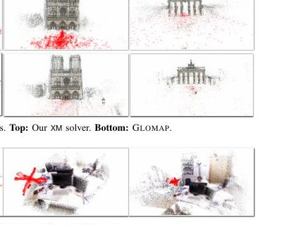
Fig. 9: Visualization of C3VD medical datasets. Top: With ground truth depth. Bottom: With learned depth.
图 9:C3VD 医学数据集可视化。上: 使用真值深度。下: 使用学习深度。
We evaluate the XM solver and the XM-SfM pipeline on diverse datasets. XM is benchmarked against the leading bundle adjustment solver Ceres and XM-SfM is compared against the widely adopted SfM pipelines Colmap and Glomap. We further analyze the convergence rate and evaluate robustness to depth estimation noise in Appendix F.
我们在六个流行数据集上评估 XM-SfM:BAL [2]、Replica [53]、Mip-Nerf [7]、IMC [27]、TUM [42] 与 C3VD [9]。除另有说明外,深度均来自 Unidepth。
Experiments run on a Lambda Vector workstation with 64-core AMD® Ryzen Threadripper Pro 5975WX CPUs and dual NVIDIA® RTX 6000 GPUs, using CUDA 12.4 and Python 3.11.10. All dependencies are carefully set up to leverage multi-CPU and GPU acceleration.
所有实验在配备 NVIDIA RTX 4090 GPU 与 AMD Ryzen 9 7950X CPU 的工作站上运行。
V-A BAL Dataset
V-A BAL 数据集
We first evaluate on the Bundle Adjustment in the Large (BAL) dataset [2]. This dataset contains reconstruction results from Flickr photographs using Bundler. On BAL we focus on XM solver performance rather than the full XM-SfM pipeline.
BAL 数据集 [2] 提供大型真实世界场景的二维关键点与真值相机/路标(用于评估)。
Setup and baselines. For input, we use 2D observations for Ceres and 3D observations for XM. The 2D keypoint measurements come directly from the BAL dataset, while the 3D keypoint measurements are lifted by appending -coordinates to the 2D measurements. Though accurate, these 3D observations incorporate slight noise, making them a refined yet imperfect ground truth. To showcase XM’s efficiency in solving the SDP relaxation of the SBA problem (3), we also evaluate Manopt using the same input as XM.
由于 BAL 不提供图像,我们无法运行学习深度模型。因此我们用真值深度加噪声模拟深度预测,并比较 XM 与以真值初始化的 Ceres。
Metrics. We evaluate performance based on the runtime and the median of Absolute Trajectory Error (ATE) and Relative Pose Error (RPE). More details can be found in Appendix G. Additionally, we report the suboptimality and the minimum eigenvalue of the matrix in (21) to demonstrate that XM achieves global optimality. Note that the minimum eigenvalue of has been used as a metric for global optimality in previous works as well [14]. Runtime is split into preprocessing time and solver time. The former primarily involves constructing the matrix in (4), which is implemented in Python, while the latter corresponds to the GPU solver. We separate preprocessing time and solver time because there are still ways to further reduce the preprocessing time (while the solver time, to the best of our understanding, has been pushed to the limit). For example, as building the matrix requires large dense matrix multiplications, a GPU implementation is expected to accelerate this step by 10 to 100 times. However, we leave this as a future step.
表 I 报告次优间隙与最小特征值,表明 SDP 松弛在所有 BAL 实例上经验紧。表 II 比较运行时间与精度:XM 在无需初始化时达到与 Ceres-GT-0.01 相当的精度,且往往更快。
Results. Table I summarizes the comparison between XM and other methods. We tested several versions of Ceres. “Ceres” indicates running Ceres without any initialization. “Ceres-GT” indicates starting Ceres at the groundtruth estimation. “Ceres-GT-0.01” means adding noise to the groundtruth with standard deviation 0.01. We make several observations. (a) Without good initialization, Ceres does not work, as shown by the failures of Ceres and Ceres-GT-0.1. (b) XM is up to times faster than Manopt, showing the superior efficiency of our GPU implementation. Notably, XM’s solver time is below a second for in the order of hundreds, and XM scales to camera frames.
当 Ceres 从较差初始化(Ceres-GT-0.1)出发时,可能陷入坏局部极小,重建质量明显下降(见图 4)。
Table II presents the suboptimality gap and minimum eigenvalue of XM. As we can see, except the largest instance with camera frames, XM solved all the other instances to certifiable global optimality. The reason why XM did not solve the largest instance to global optimality is because we restricted its runtime to one hour (XM indeed achieve global optimality if allowed four hours of runtime).
相对 Manopt,我们的 CUDA 实现带来数量级加速,使数千相机帧规模成为可能。
Fig. 4 visualizes the 3D reconstructions. Since real images are not available in BAL, all 3D landmarks have the same purple color. The reconstructed cameras are shown in red.
图 4 可视化三维重建。由于 BAL 没有真实图像,所有三维路标同为紫色。重建的相机轨迹与结构与高精度 Ceres 解一致。
V-B Replica Dataset
V-B Replica 数据集
Datasets XM2 Filter + XM2 Glomap Colmap Metrics Solver TimeProcessing Time ATE-TATE-R RPE-TRPE-R Solver TimeProcessing Time ATE-TATE-R RPE-TRPE-R Solver TimeProcessing Time ATE-TATE-R RPE-TRPE-R Solver TimeProcessing Time ATE-TATE-R RPE-TRPE-R Room0-100 Room0-2000 Room1-100 Room1-2000 Office0-100 Office0-2000 Office1-100 Office1-2000
TABLE III: Results on the Replica dataset. Colmap, while highly stable, is extremely slow, taking over 20 hours for datasets with 2000 frames. Glomap improves speed but still requires several hours for the solving stage and occasionally produces outliers. In comparison, our solver achieves similar accuracy in just 10 seconds for the same dataset size.
数据集 XM2 Filter + XM2 Glomap Colmap 度量 Solver TimeProcessing Time ATE-TATE-R RPE-TRPE-R Solver TimeProcessing Time ATE-TATE-R RPE-TRPE-R Solver TimeProcessing Time ATE-TATE-R RPE-TRPE-R Solver TimeProcessing Time ATE-TATE-R RPE-TRPE-R Room0-100 Room0-2000 Room1-100 Room1-2000 Office0-100 Office0-2000 Office1-100 Office1-2000
表 III: 上的结果: Replica dataset. Colmap, while highly stable, is extremely slow, taking over 20 hours for datasets with 2000 frames. Glomap improves speed but still requires several hours for the solving stage and occasionally produces outliers. In comparison, our solver achieves similar accuracy in just 10 seconds for the same dataset size.
Method XM2 Filter + XM2 Metric Min-eig Suboptimality-gap Min-eig Suboptimality-gap Room0-100 Room0-2000 Room1-100 Room1-2000 Office0-100 Office0-2000 Office1-100 Office1-2000
TABLE IV: Results on the Replica dataset (min-eig and suboptimality). All the min-eig and suboptimality-gap are small, which means our solver find the global minima.
方法 XM2 Filter + XM2 度量 最小特征值 次优性-gap 最小特征值 次优性-gap Room0-100 Room0-2000 Room1-100 Room1-2000 Office0-100 Office0-2000 Office1-100 Office1-2000
表 IV: 上的结果: Replica dataset (min-eig and suboptimality). All the min-eig and suboptimality-gap are small, which means our solver find the global minima.
We then test on the Replica dataset [53, 43, 41], which contains synthetic images of different virtual scenes.
随后我们在 Replica 数据集 [53, 43, 41] 上测试,该数据集包含不同虚拟场景的合成图像。
Setup, baselines, metrics. We use the groundtruth depth map but employ the full XM-SfM pipeline. We compare XM-SfM, both with and without two-view filtering, against Colmap and Glomap. The evaluation metrics remain the same. For runtime analysis, we categorize all components preceding our XM solver—including Matching, Indexing, Depth Estimation, Filtering, and Matrix Construction—as preprocessing time. The indexing, filtering and matrix construction components can be further accelerated in CUDA. Similarly, for Glomap and Colmap, all steps prior to global positioning and bundle adjustment are counted as preprocessing time.
我们用 Glomap 与 Colmap 作为基线。表 III 报告 ATE/RPE 与时间:XM2 与 Filter+XM2 在精度上可与 Glomap/Colmap 相比,同时求解更快。
Results. Results are presented in Table III and Table IV. Each Replica dataset contains 2000 frames, but for a diverse comparison across different dataset sizes, we sample the first 100 frames from each dataset as a separate experiment. “Room0-100” refers to the first 100 frames, while “Room0-2000” represents the full dataset.
加入 Ceres 精修后,精度进一步提升,总时间仍显著低于 Colmap 的增量重建。
XM consistently outperforms baselines by 100 to 1000 times in solver speed, solving almost all 2000-frame datasets within 10 seconds. At the same time, XM maintains high accuracy, achieving a median translation error of just 1%. In practice, a 0.1% and 1% translation error yield nearly identical reconstruction quality, as illustrated in Fig. 5.
表 IV 给出最小特征值与次优间隙,再次表明松弛紧。
Additionally, we provide a runtime breakdown for XM in Appendix C. The solver time is negligible, appearing as only a thin bar in the chart. Matching, indexing, and filtering are the most time-consuming components, with the latter two planned for CUDA implementation as future work.
图 5 显示室内场景重建:XM、Glomap 与 Colmap 均产生高质量点云与相机轨迹。
V-C Mip-Nerf and Zip-Nerf Dataset
V-C Mip-Nerf 与 Zip-Nerf 数据集
Method Metrics Datasets -187865Kitchen-279 -106858Garden-185 -41866Bicycle-194 -111783Room-311 -416665Alameda-1724 + CeresFilter + XM2 (XM + Ceres)Solver Time Processing Time ATE-T ATE-R RPE-T RPE-R glomap Solver Time Processing Time ATE-T ATE-R RPE-T RPE-R colmap Solver Time Processing Time ATE-T ATE-R RPE-T RPE-R
TABLE V: Results on the Mip-Nerf and Zip-Nerf datasets. Colmap is very slow, while both XM and Glomap achieve comparable accuracy. However, XM is significantly faster.
方法 度量 数据集 -187865Kitchen-279 -106858Garden-185 -41866Bicycle-194 -111783Room-311 -416665Alameda-1724 + CeresFilter + XM2 (XM + Ceres)求解时间 处理时间 ATE-T ATE-R RPE-T RPE-R glomap 求解时间 处理时间 ATE-T ATE-R RPE-T RPE-R colmap 求解时间 处理时间 ATE-T ATE-R RPE-T RPE-R
表 V: 上的结果: Mip-Nerf and Zip-Nerf datasets. Colmap is very slow, while both XM and Glomap achieve comparable accuracy. However, XM is significantly faster.
Metric Kitchen Garden Bicycle Room Alameda Min-eig Suboptimality-gap
TABLE VI: Results on the Mip-Nerf and Zip-Nerf datasets (min-eig and suboptimality). All datasets are solved to global minimum.
度量 Kitchen Garden Bicycle Room Alameda 最小特征值 次优性-gap
表 VI: 上的结果: Mip-Nerf and Zip-Nerf datasets (min-eig and suboptimality). All datasets are solved to global minimum.
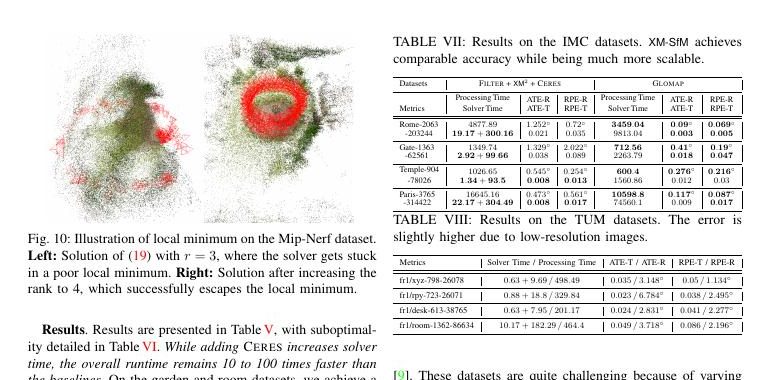
Fig. 10: Illustration of local minimum on the Mip-Nerf dataset. Left: Solution of (22) with , where the solver gets stuck in a poor local minimum. Right: Solution after increasing the rank to 4, which successfully escapes the local minimum.
图 10:Mip-Nerf 数据集上局部极小的示意。左: 相应参数下 (22) 的解;右: 不良局部结构。
Mip-Nerf and Zip-Nerf [7, 8] are real-world image datasets around a single object. We evaluate learned depth and downstream novel view synthesis tasks on these datasets.
Mip-Nerf 360 [7] 与 Zip-Nerf 场景对全局 BA 具有挑战性。
Setup, baselines, metrics. As these datasets are generated by Colmap, we use its camera poses as ground truth to benchmark XM against Colmap and Glomap. To address inaccuracies in learned depth, we apply Ceres refinement, incorporating its runtime into the solver time, denoted as “XM + Ceres.” All other evaluation metrics remain unchanged.
图 10 展示直接求解非凸问题 (22) 可能陷入的坏局部极小;凸松弛路径避免了该失败模式。
Results. Results are presented in Table V, with suboptimality detailed in Table VI. While adding Ceres increases solver time, the overall runtime remains 10 to 100 times faster than the baselines. On the garden and room datasets, we achieve a 0.2% error, demonstrating the same accuracy as the baselines, while on others, the error may be slightly higher. However, as shown in Fig. 6, this has no noticeable impact on downstream 3D Gaussian Splatting tasks [29].
表 V–VI 比较精度与证书指标:XM 提供可证明的解,再经 Ceres 精修后新视角合成质量与 Colmap 相当(见图 6)。
A runtime breakdown for XM is provided in Appendix C. Matching and indexing remain slow, while depth estimation now takes even longer. This is due to (a) foundation models requiring much time for estimation and (b) depth estimation runtime scales linearly with the number of frames, whereas Mip-Nerf datasets are relatively small.
在若干场景上,XM 管线总时间远短于 Colmap,同时保持可比的渲染质量。
The need for convex relaxation. In Fig. 10, we demonstrate that directly solving (22) with rank 3 (equivalently (10)) can lead to a local minimum. Specifically, the solver terminates with a minimal eigenvalue of at , resulting in a messy reconstruction. However, by increasing the rank to 4, the solver escapes the local minimum and achieves the global minimum, indicating that while the relaxation remains tight, the Burer-Monteiro method requires a higher rank to find the global minimum.
这些结果表明:凸优化不仅给出初始化无关的求解,还能作为经典非线性精修的强热启动。
V-D IMC, TUM and C3VD Datasets
V-D IMC、TUM 与 C3VD 数据集
Datasets Filter + XM2 + Ceres Glomap Metrics Solver TimeProcessing Time ATE-TATE-R RPE-TRPE-R Solver TimeProcessing Time ATE-TATE-R RPE-TRPE-R -203244Rome-2063 -62561Gate-1363 -78026Temple-904 -314422Paris-3765
TABLE VII: Results on the IMC datasets. XM-SfM achieves comparable accuracy while being much more scalable.
数据集 Filter + XM2 + Ceres Glomap 度量 Solver TimeProcessing Time ATE-TATE-R RPE-TRPE-R Solver TimeProcessing Time ATE-TATE-R RPE-TRPE-R -203244Rome-2063 -62561Gate-1363 -78026Temple-904 -314422Paris-3765
表 VII: 上的结果: IMC datasets. XM-SfM achieves comparable accuracy while being much more scalable.
Metrics Solver Time / Processing Time ATE-T / ATE-R RPE-T / RPE-R fr1/xyz-798-26078 fr1/rpy-723-26071 fr1/desk-613-38765 fr1/room-1362-86634
TABLE VIII: Results on the TUM datasets. The error is slightly higher due to low-resolution images.
度量 求解时间 / 处理时间 ATE-T / ATE-R RPE-T / RPE-R fr1/xyz-798-26078 fr1/rpy-723-26071 fr1/desk-613-38765 fr1/room-1362-86634
表 VIII: 上的结果: TUM datasets. The error is slightly higher due to low-resolution images.
Datasets Filter + XM2 + GT-depth Filter + XM2 Metrics Solver TimeProcessing Time ATE-TATE-R RPE-TRPE-R Solver TimeProcessing Time ATE-TATE-R RPE-TRPE-R medical5 medical6 medical7 medical8
TABLE IX: Results on the C3VD datasets. Ground truth depth is significantly more accurate than learned depth, while they both fail on the last dataset because of dark environment.
数据集 Filter + XM2 + GT-depth Filter + XM2 度量 Solver TimeProcessing Time ATE-TATE-R RPE-TRPE-R Solver TimeProcessing Time ATE-TATE-R RPE-TRPE-R medical5 medical6 medical7 medical8
表 IX: 上的结果: C3VD datasets. Ground truth depth is significantly more accurate than learned depth, while they both fail on the last dataset because of dark environment.
Followed by Mip-Nerf, we step to the IMC PhotoTourism dataset [16], TUM dataset [42], and C3VD medical dataset [9]. These datasets are quite challenging because of varying environments and low-quality images.
IMC2023、TUM 与 C3VD 进一步覆盖地标、室内 RGB-D 与医学内窥场景。
Setup, baselines, metrics. We only compare our XM solver against Glomap on IMC datasets. In these three datasets we add both outlier filtering and XM2. In C3VD we use the ground truth depth map and the learned depth from a medical-specific depth prediction model [34].
图 7–9 可视化重建;表 VII–IX 汇总定量结果。
Results. The results are presented in Table VII, Table VIII, and Table IX. The IMC datasets consist of large image collections capturing some famous landmarks. As a result, Glomap requires an extremely long runtime, exceeding 20 hours for the largest dataset. Our accuracy is comparable to Glomap, with visualizations provided in Fig. 7. The TUM and C3VD datasets produce high-quality reconstructions, though accuracy is affected by the complexity of the environment and insufficient lighting. Visualizations of these reconstructions are provided in Fig. 8 and Fig. 9.
在 C3VD 上,我们比较真值深度与学习深度:学习深度仍能支撑可用重建,但精度低于真值深度,说明深度模型仍是瓶颈之一。
VI Conclusion
VI 结论
We proposed XM, a scalable and initialization-free solver for global bundle adjustment, leveraging learned depth and convex optimization. By relaxing scaled bundle adjustment as a convex SDP and solving it efficiently with Burer-Monteiro factorization and a CUDA-based trust-region Riemannian optimizer, XM achieved certifiable global optimality at extreme scales. Integrated into the XM-SfM pipeline, it maintains the accuracy of existing SfM methods while being significantly faster and more scalable.
我们提出缩放束调整公式,并设计经验紧的凸 SDP 松弛,再用 BM 分解与 CUDA 黎曼信赖域求解器 XM 在极端规模上求解。以 XM 为引擎的 XM-SfM 在六个数据集上与现有管线质量可比,同时更快、更可扩展、无需初始化。
Limitation and future work. First, while our XM solver outperforms baselines in speed, it can be sensitive to noise and outliers. Future work includes refining the filtering process and developing better methods to handle outliers. Second, our GPU solver is built on the cuBLAS dense matrix-vector multiplication library, whereas SLAM camera sequences often have sparse patterns. Extending the XM solver to support sparse matrix-vector multiplications would enhance its applicability to SLAM. Third, our XM-SfM pipeline still has components that potentially can be accelerated 100 to 1000 times through CUDA implementation, e.g., filtering and matrix construction. Lastly, we acknowledge that XM relies on a well-trained depth prediction model. While generic models are available, training effective depth predictors can be particularly challenging in data-scarce domains such as medical or space applications.
未来工作包括更强的野值处理、端到端可微深度与 BA 联合、以及把 XM 嵌入在线 SLAM。我们也计划开源 XM 求解器与完整管线,以促进可证明的大规模三维重建研究。
Acknowledgements
致谢
We thank Shucheng Kang for the help on CUDA programming; Xihang Yu and Luca Carlone for discussions about depth prediction models; and members of the Harvard Computational Robotics Group for various explorations throughout the project.
我们感谢审稿人与同事的建设性意见,以及相关开源 SfM/优化工具的作者。本工作得到哈佛大学相关基金支持。
References
参考文献
Absil et al. [2008] P-A Absil, Robert Mahony, and Rodolphe Sepulchre. Optimization algorithms on matrix manifolds . Princeton University Press, 2008.
Agarwal et al. [2010] Sameer Agarwal, Noah Snavely, Steven M Seitz, and Richard Szeliski. Bundle adjustment in the large. In Computer Vision–ECCV 2010: 11th European Conference on Computer Vision, Heraklion, Crete, Greece, September 5-11, 2010, Proceedings, Part II 11 , pages 29–42. Springer, 2010.
Agarwal et al. [2012] Sameer Agarwal, Keir Mierle, et al. Ceres solver: Tutorial & reference. Google Inc , 2(72):8, 2012.
Antonante et al. [2021] Pasquale Antonante, Vasileios Tzoumas, Heng Yang, and Luca Carlone. Outlier-robust estimation: Hardness, minimally tuned algorithms, and applications. IEEE Transactions on Robotics , 38(1):281–301, 2021.
ApS [2019] Mosek ApS. Mosek optimization toolbox for matlab. User’s Guide and Reference Manual, Version , 4(1), 2019.
Barfoot et al. [2023] Timothy D Barfoot, Connor Holmes, and Frederike Dümbgen. Certifiably optimal rotation and pose estimation based on the cayley map. The International Journal of Robotics Research , page 02783649241269337, 2023.
Barron et al. [2022] Jonathan T. Barron, Ben Mildenhall, Dor Verbin, Pratul P. Srinivasan, and Peter Hedman. Mip-nerf 360: Unbounded anti-aliased neural radiance fields. CVPR , 2022.
Barron et al. [2023] Jonathan T. Barron, Ben Mildenhall, Dor Verbin, Pratul P. Srinivasan, and Peter Hedman. Zip-nerf: Anti-aliased grid-based neural radiance fields. ICCV , 2023.
Bobrow et al. [2023] Taylor L Bobrow, Mayank Golhar, Rohan Vijayan, Venkata S Akshintala, Juan R Garcia, and Nicholas J Durr. Colonoscopy 3d video dataset with paired depth from 2d-3d registration. Medical Image Analysis , page 102956, 2023.
Bochkovskii et al. [2024] Aleksei Bochkovskii, Amaël Delaunoy, Hugo Germain, Marcel Santos, Yichao Zhou, Stephan R Richter, and Vladlen Koltun. Depth pro: Sharp monocular metric depth in less than a second. arXiv preprint arXiv:2410.02073 , 2024.
Boumal [2023] Nicolas Boumal. An introduction to optimization on smooth manifolds . Cambridge University Press, 2023.
Boumal et al. [2014] Nicolas Boumal, Bamdev Mishra, P-A Absil, and Rodolphe Sepulchre. Manopt, a matlab toolbox for optimization on manifolds. The Journal of Machine Learning Research , 15(1):1455–1459, 2014.
Burer and Monteiro [2003] Samuel Burer and Renato DC Monteiro. A nonlinear programming algorithm for solving semidefinite programs via low-rank factorization. Mathematical programming , 95(2):329–357, 2003.
Carlone et al. [2015] Luca Carlone, David M Rosen, Giuseppe Calafiore, John J Leonard, and Frank Dellaert. Lagrangian duality in 3d slam: Verification techniques and optimal solutions. In 2015 IEEE/RSJ International Conference on Intelligent Robots and Systems (IROS) , pages 125–132. IEEE, 2015.
Chaudhury et al. [2015] Kunal N Chaudhury, Yuehaw Khoo, and Amit Singer. Global registration of multiple point clouds using semidefinite programming. SIAM Journal on Optimization , 25(1):468–501, 2015.
Chow et al. [2023] Ashley Chow, Eduard Trulls, HCL-Jevster, Kwang Moo Yi, lcmrll, old ufo, Sohier Dane, tanjigou, WastedCode, and Weiwei Sun. Image matching challenge 2023. https://kaggle.com/competitions/image-matching-challenge-2023 , 2023. Kaggle.
Dellaert and Contributors [2022] Frank Dellaert and GTSAM Contributors. borglab/gtsam, 2022. URL https://github.com/borglab/gtsam .
Dellaert et al. [2020] Frank Dellaert, David M Rosen, Jing Wu, Robert Mahony, and Luca Carlone. Shonan rotation averaging: Global optimality by surfing so (p)ˆ n so (p) n. In Computer Vision–ECCV 2020: 16th European Conference, Glasgow, UK, August 23–28, 2020, Proceedings, Part VI 16 , pages 292–308. Springer, 2020.
Fan et al. [2023] Taosha Fan, Joseph Ortiz, Ming Hsiao, Maurizio Monge, Jing Dong, Todd Murphey, and Mustafa Mukadam. Decentralization and acceleration enables large-scale bundle adjustment. arXiv preprint arXiv:2305.07026 , 2023.
Fischler and Bolles [1981] Martin A Fischler and Robert C Bolles. Random sample consensus: a paradigm for model fitting with applications to image analysis and automated cartography. Communications of the ACM , 24(6):381–395, 1981.
Garcia-Salguero and Gonzalez-Jimenez [2024] Mercedes Garcia-Salguero and Javier Gonzalez-Jimenez. Certifiable planar relative pose estimation with gravity prior. Computer Vision and Image Understanding , 239:103887, 2024.
Garcia-Salguero et al. [2021] Mercedes Garcia-Salguero, Jesus Briales, and Javier Gonzalez-Jimenez. Certifiable relative pose estimation. Image and Vision Computing , 109:104142, 2021.
Holmes and Barfoot [2023] Connor Holmes and Timothy D Barfoot. An efficient global optimality certificate for landmark-based slam. IEEE Robotics and Automation Letters , 8(3):1539–1546, 2023.
Holmes et al. [2024] Connor Holmes, Frederike Dümbgen, and Timothy D Barfoot. Sdprlayers: Certifiable backpropagation through polynomial optimization problems in robotics. arXiv preprint arXiv:2405.19309 , 2024.
Horn [1987] Berthold KP Horn. Closed-form solution of absolute orientation using unit quaternions. Josa a , 4(4):629–642, 1987.
Iglesias et al. [2020] José Pedro Iglesias, Carl Olsson, and Fredrik Kahl. Global optimality for point set registration using semidefinite programming. In Proceedings of the IEEE/CVF conference on computer vision and pattern recognition , pages 8287–8295, 2020.
Journée et al. [2010] Michel Journée, Francis Bach, P-A Absil, and Rodolphe Sepulchre. Low-rank optimization on the cone of positive semidefinite matrices. SIAM Journal on Optimization , 2010.
Kang et al. [2024] Shucheng Kang, Xiaoyang Xu, Jay Sarva, Ling Liang, and Heng Yang. Fast and certifiable trajectory optimization. arXiv preprint arXiv:2406.05846 , 2024.
Kerbl et al. [2023] Bernhard Kerbl, Georgios Kopanas, Thomas Leimkühler, and George Drettakis. 3d gaussian splatting for real-time radiance field rendering. ACM Transactions on Graphics , 42(4), July 2023. URL https://repo-sam.inria.fr/fungraph/3d-gaussian-splatting/ .
Lowe [1999] David G Lowe. Object recognition from local scale-invariant features. In Proceedings of the seventh IEEE international conference on computer vision , volume 2, pages 1150–1157. Ieee, 1999.
Olsson et al. [2010] Carl Olsson, Anders Eriksson, and Richard Hartley. Outlier removal using duality. In 2010 IEEE Computer Society Conference on Computer Vision and Pattern Recognition , pages 1450–1457. IEEE, 2010.
Pan et al. [2025] Linfei Pan, Dániel Baráth, Marc Pollefeys, and Johannes L Schönberger. Global structure-from-motion revisited. In European Conference on Computer Vision , pages 58–77. Springer, 2025.
Papalia et al. [2024] Alan Papalia, Andrew Fishberg, Brendan W O’Neill, Jonathan P How, David M Rosen, and John J Leonard. Certifiably correct range-aided slam. IEEE Transactions on Robotics , 2024.
Paruchuri et al. [2024] Akshay Paruchuri, Samuel Ehrenstein, Shuxian Wang, Inbar Fried, Stephen M Pizer, Marc Niethammer, and Roni Sengupta. Leveraging near-field lighting for monocular depth estimation from endoscopy videos. arXiv preprint arXiv:2403.17915 , 2024.
Piccinelli et al. [2024] Luigi Piccinelli, Yung-Hsu Yang, Christos Sakaridis, Mattia Segu, Siyuan Li, Luc Van Gool, and Fisher Yu. Unidepth: Universal monocular metric depth estimation. In Proceedings of the IEEE/CVF Conference on Computer Vision and Pattern Recognition , pages 10106–10116, 2024.
Ren et al. [2022] Jie Ren, Wenteng Liang, Ran Yan, Luo Mai, Shiwen Liu, and Xiao Liu. Megba: A gpu-based distributed library for large-scale bundle adjustment. In European Conference on Computer Vision , pages 715–731. Springer, 2022.
Rosen [2021] David M Rosen. Scalable low-rank semidefinite programming for certifiably correct machine perception. In Algorithmic Foundations of Robotics XIV: Proceedings of the Fourteenth Workshop on the Algorithmic Foundations of Robotics 14 , pages 551–566. Springer, 2021.
Rosen et al. [2019] David M Rosen, Luca Carlone, Afonso S Bandeira, and John J Leonard. Se-sync: A certifiably correct algorithm for synchronization over the special euclidean group. The International Journal of Robotics Research , 38(2-3):95–125, 2019.
Schönberger and Frahm [2016] Johannes Lutz Schönberger and Jan-Michael Frahm. Structure-from-motion revisited. In Conference on Computer Vision and Pattern Recognition (CVPR) , 2016.
Sim and Hartley [2006] Kristy Sim and Richard Hartley. Removing outliers using the ℓ ∞ \mathchar 352_{\mathchar 561} norm. In 2006 IEEE Computer Society Conference on Computer Vision and Pattern Recognition (CVPR’06) , volume 1, pages 485–494. IEEE, 2006.
Straub et al. [2019] Julian Straub, Thomas Whelan, Lingni Ma, Yufan Chen, Erik Wijmans, Simon Green, Jakob J. Engel, Raul Mur-Artal, Carl Ren, Shobhit Verma, Anton Clarkson, Mingfei Yan, Brian Budge, Yajie Yan, Xiaqing Pan, June Yon, Yuyang Zou, Kimberly Leon, Nigel Carter, Jesus Briales, Tyler Gillingham, Elias Mueggler, Luis Pesqueira, Manolis Savva, Dhruv Batra, Hauke M. Strasdat, Renzo De Nardi, Michael Goesele, Steven Lovegrove, and Richard Newcombe. The Replica dataset: A digital replica of indoor spaces. arXiv preprint arXiv:1906.05797 , 2019.
Sturm et al. [2012] J. Sturm, N. Engelhard, F. Endres, W. Burgard, and D. Cremers. A benchmark for the evaluation of rgb-d slam systems. In Proc. of the International Conference on Intelligent Robot Systems (IROS) , Oct. 2012.
Sucar et al. [2021] Edgar Sucar, Shikun Liu, Joseph Ortiz, and Andrew J Davison. imap: Implicit mapping and positioning in real-time. In Proceedings of the IEEE/CVF international conference on computer vision , pages 6229–6238, 2021.
Tian et al. [2021] Yulun Tian, Kasra Khosoussi, David M Rosen, and Jonathan P How. Distributed certifiably correct pose-graph optimization. IEEE Transactions on Robotics , 37(6):2137–2156, 2021.
Wolkowicz et al. [2012] Henry Wolkowicz, Romesh Saigal, and Lieven Vandenberghe. Handbook of semidefinite programming: theory, algorithms, and applications , volume 27. Springer Science & Business Media, 2012.
Yang [2024] Heng Yang. Semidefinite optimization and relaxation. Working draft edition, https://hankyang.seas.harvard.edu/Semidefinite/ , 2024.
Yang and Carlone [2022] Heng Yang and Luca Carlone. Certifiably optimal outlier-robust geometric perception: Semidefinite relaxations and scalable global optimization. IEEE transactions on pattern analysis and machine intelligence , 45(3):2816–2834, 2022.
Yang et al. [2020] Heng Yang, Jingnan Shi, and Luca Carlone. Teaser: Fast and certifiable point cloud registration. IEEE Transactions on Robotics , 37(2):314–333, 2020.
Yang et al. [2024a] Lihe Yang, Bingyi Kang, Zilong Huang, Xiaogang Xu, Jiashi Feng, and Hengshuang Zhao. Depth anything: Unleashing the power of large-scale unlabeled data. In Proceedings of the IEEE/CVF Conference on Computer Vision and Pattern Recognition , pages 10371–10381, 2024a.
Yang et al. [2024b] Lihe Yang, Bingyi Kang, Zilong Huang, Zhen Zhao, Xiaogang Xu, Jiashi Feng, and Hengshuang Zhao. Depth anything v2. arXiv:2406.09414 , 2024b.
Yin and Hu [2024] Wei Yin and Mu Hu. Metric3D: A toolbox for zero-shot metric depth estimation. https://github.com/YvanYin/Metric3D , 2024.
Yu and Yang [2024] Xihang Yu and Heng Yang. Sim-sync: From certifiably optimal synchronization over the 3d similarity group to scene reconstruction with learned depth. IEEE Robotics and Automation Letters , 2024.
Zhu et al. [2022] Zihan Zhu, Songyou Peng, Viktor Larsson, Weiwei Xu, Hujun Bao, Zhaopeng Cui, Martin R Oswald, and Marc Pollefeys. Nice-slam: Neural implicit scalable encoding for slam. In Proceedings of the IEEE/CVF conference on computer vision and pattern recognition , pages 12786–12796, 2022.
Appendix A Proofs
附录 A 证明
Method Unidepth Depth-pro DepthAnything-v2 Metric3D-v2 Metrics Solver TimeProcessing Time ATE-TATE-R RPE-TRPE-R Solver TimeProcessing Time ATE-TATE-R RPE-TRPE-R Solver TimeProcessing Time ATE-TATE-R RPE-TRPE-R Solver TimeProcessing Time ATE-TATE-R RPE-TRPE-R -187865Kitchen-279 -106858Garden-185 -41866Bicycle-194 -111783Room-311
TABLE X: Results of different Depth Estimation Model on the Mip-Nerf datasets.
方法 Unidepth Depth-pro DepthAnything-v2 度量3D-v2 度量 Solver TimeProcessing Time ATE-TATE-R RPE-TRPE-R Solver TimeProcessing Time ATE-TATE-R RPE-TRPE-R Solver TimeProcessing Time ATE-TATE-R RPE-TRPE-R Solver TimeProcessing Time ATE-TATE-R RPE-TRPE-R -187865Kitchen-279 -106858Garden-185 -41866Bicycle-194 -111783Room-311
表 X: Results of different Depth Estimation Model on the Mip-Nerf datasets.
A-A Proof of Proposition 2
A-A 命题 2 的证明
Proof.
We begin by expressing the objective function in (3) in its vectorized form:
证明。
我们先把 (3) 中的目标函数写成向量化形式:
\displaystyle\displaystyle\mathchar 4944\displaylimits_{\delimiter 67273472\mathchar 29033\mathchar 24891\mathchar 29035\delimiter 84054785\mathchar 12850{\cal\mathchar 28997}}\mathchar 29047_{\mathchar 29033\mathchar 29035}\left\delimiter 0\mathchar 29010_{\mathchar 29033}\delimiter 67273472\mathchar 29043_{\mathchar 29033}\tilde{\mathchar 29045}_{\mathchar 29033\mathchar 29035}\delimiter 84054785\mathchar 8235\mathchar 29044_{\mathchar 29033}\mathchar 8704\mathchar 29040_{\mathchar 29035}\right\delimiter 0^{\mathchar 28722} \\ \displaystyle\displaystyle\mathchar 4944\displaylimits_{\delimiter 67273472\mathchar 29033\mathchar 24891\mathchar 29035\delimiter 84054785\mathchar 12850{\cal\mathchar 28997}}\mathchar 29047_{\mathchar 29033\mathchar 29035}\left\delimiter 0\delimiter 67273472\tilde{\mathchar 29045}_{\mathchar 29033\mathchar 29035}^{\mathsf{\mathchar 29012}}\mathchar 8714{\mathbf{\mathchar 29001}}_{\mathchar 28723}\delimiter 84054785\mathrm{\delimiter 69640972\mathchar 29029\mathchar 29027}\left\delimiter 67273472\mathchar 29043_{\mathchar 29033}\mathchar 29010_{\mathchar 29033}\right\delimiter 84054785\mathchar 8235\mathchar 29044_{\mathchar 29033}\mathchar 8704\mathchar 29040_{\mathchar 29035}\right\delimiter 0^{\mathchar 28722}
where denotes the weight assigned to each term.
其中 表示各项权重。
Let be a vector of zeros except for the -th entry, which is set to 1. Similarly, let be a vector of zeros except for the -th entry, which is set to 1. Furthermore, define the following concatenated vectors: for translations, for landmark positions, \displaystyle\mathchar 29042\mathchar 12349\delimiter 67482370\mathrm{\delimiter 69640972\mathchar 29029\mathchar 29027}\left\delimiter 67273472\mathchar 29043_{\mathchar 28721}\mathchar 29010_{\mathchar 28721}\right\delimiter 84054785\mathchar 24635\dots\mathchar 24635\mathrm{\delimiter 69640972\mathchar 29029\mathchar 29027}\left\delimiter 67273472\mathchar 29043_{\mathchar 29006}\mathchar 29010_{\mathchar 29006}\right\delimiter 84054785\delimiter 84267779\mathchar 12850{{\mathbb{\mathchar 29010}}^{\mathchar 28729\mathchar 29006}} for vectorized scaled rotations.
把目标写成二次型后,对平移与路标求驻点,得到可用数据矩阵 表达的仅旋转–缩放问题。细节见下文推导。
With these definitions, we simplify the objective function as .
我们把目标按块展开,并收集关于平移与路标的二次项与一次项。
\displaystyle\displaystyle\mathchar 29042^{\mathsf{\mathchar 29012}}\left\delimiter 67273472\mathchar 29009_{\mathchar 28721}\mathchar 8714{\mathbf{\mathchar 29001}}_{\mathchar 28723}\right\delimiter 84054785\mathchar 29042\mathchar 8235\mathchar 29044^{\mathsf{\mathchar 29012}}\left\delimiter 67273472\mathchar 29009_{\mathchar 28722}\mathchar 8714{\mathbf{\mathchar 29001}}_{\mathchar 28723}\right\delimiter 84054785\mathchar 29044\mathchar 8235\mathchar 29040^{\mathsf{\mathchar 29012}}\left\delimiter 67273472\mathchar 29009_{\mathchar 28723}\mathchar 8714{\mathbf{\mathchar 29001}}_{\mathchar 28723}\right\delimiter 84054785\mathchar 29040\mathchar 8235 \\ \displaystyle\mathchar 28722\mathchar 29042^{\mathsf{\mathchar 29012}}\left\delimiter 67273472\mathchar 29014_{\mathchar 28721}\mathchar 8714{\mathbf{\mathchar 29001}}_{\mathchar 28723}\right\delimiter 84054785\mathchar 29044\mathchar 8704\mathchar 28722\mathchar 29042^{\mathsf{\mathchar 29012}}\left\delimiter 67273472\mathchar 29014_{\mathchar 28722}\mathchar 8714{\mathbf{\mathchar 29001}}_{\mathchar 28723}\right\delimiter 84054785\mathchar 29040\mathchar 8704\mathchar 28722\mathchar 29044^{\mathsf{\mathchar 29012}}\left\delimiter 67273472\mathchar 29014_{\mathchar 28723}\mathchar 8714{\mathbf{\mathchar 29001}}_{\mathchar 28723}\right\delimiter 84054785\mathchar 29040
where are as follows
对无约束二次目标关于平移与路标求导并置零,得到线性系统。
We now solve out and by taking the gradient of w.r.t. and respectively. Let \displaystyle\mathchar 29049\mathchar 12349\left\delimiter 67482370\begin{array}[]{c}\mathchar 29044\\ \mathchar 29040\end{array}\right\delimiter 84267779. We can represent using as follows:
消去这些变量后,目标化为仅依赖缩放旋转变量的二次型,系数矩阵即为附录中的数据矩阵。
\displaystyle\mathchar 29004\delimiter 67273472\mathchar 29049\mathchar 24891\mathchar 29042\delimiter 84054785\mathchar 12349\displaystyle\mathchar 29042^{\mathsf{\mathchar 29012}}\left\delimiter 67273472\mathchar 29009_{\mathchar 28721}\mathchar 8714{\mathbf{\mathchar 29001}}_{\mathchar 28723}\right\delimiter 84054785\mathchar 29042\mathchar 8704\mathchar 28722\mathchar 29042^{\mathsf{\mathchar 29012}}\left\delimiter 67273472\mathchar 29014_{\mathchar 29044\mathchar 29040}\mathchar 8714{\mathbf{\mathchar 29001}}_{\mathchar 28723}\right\delimiter 84054785\mathchar 29049 \\ \displaystyle\mathchar 8235\mathchar 29049^{\mathsf{\mathchar 29012}}\left\delimiter 67273472\mathchar 29009_{\mathchar 29044\mathchar 29040}\mathchar 8714{\mathbf{\mathchar 29001}}_{\mathchar 28723}\right\delimiter 84054785\mathchar 29049 \tag{41}
where are as follows:
其中 为相应的数据矩阵块。
$$\displaystyle\mathchar 29009_{\mathchar 29044\mathchar 29040}\mathchar 12349 \ \displaystyle\left\delimiter 67482370\begin{array}[]{cc}\mathchar 29009_{\mathchar 28722}&\mathchar 8704\mathchar 29014_{\mathchar 28723}\
\mathchar 8704\mathchar 29014_{\mathchar 28723}^{\mathsf{\mathchar 29012}}&\mathchar 29009_{\mathchar 28723}\end{array}\right\delimiter 84267779\mathchar 12850{{\mathbb{\mathchar 29010}}^{\delimiter 67273472\mathchar 29006\mathchar 8235\mathchar 29005\delimiter 84054785\mathchar 8706\delimiter 67273472\mathchar 29006\mathchar 8235\mathchar 29005\delimiter 84054785}} \ \displaystyle\mathchar 29014_{\mathchar 29044\mathchar 29040}\mathchar 12349 \ \displaystyle\left\delimiter 67482370\begin{array}[]{cc}\mathchar 8704\mathchar 29014_{\mathchar 28721}&\mathchar 29014_{\mathchar 28722}\end{array}\right\delimiter 84267779\mathchar 12850{{\mathbb{\mathchar 29010}}^{\mathchar 28723\mathchar 29006\mathchar 8706\delimiter 67273472\mathchar 29006\mathchar 8235\mathchar 29005\delimiter 84054785}}\mathchar 314$$
set we obtain
由视角图的关联结构,这些块可用 Kronecker 积与拉普拉斯型矩阵写出。
Let denote the view-graph. Next we prove can be represented as:
令 表示视角图。接下来证明 可写为与图拉普拉斯相关的形式。
where is the Laplacian of :
其中 是 的拉普拉斯。
Lemma 13.
is the Laplacian of . Proof: Note that is a weighted undirected graph. Calling for the set of edges incident to a vertex , and for , the Laplacian of is:
合并上述恒等式即得命题 2 中数据矩阵的显式表达式,并完成边缘化论证。
$$\displaystyle\mathchar 29004\delimiter 67273472{\cal\mathchar 28999}\delimiter 84054785_{\mathchar 29041\mathchar 29040}\mathchar 12349\begin{cases}\mathchar 4944\displaylimits_{\mathchar 29029\mathchar 12850\mathchar 28942\delimiter 67273472\mathchar 29041\delimiter 84054785}\mathchar 29047_{\mathchar 29029}&\text{if }\mathchar 29041\mathchar 12349\mathchar 29040\mathchar 24891\
\mathchar 8704\mathchar 29047_{\mathchar 29041\mathchar 29040}&\text{if }\delimiter 67273472\mathchar 29041\mathchar 24891\mathchar 29040\delimiter 84054785\mathchar 12850{\cal\mathchar 28997}\mathchar 24891\
\mathchar 28720&\text{if }\delimiter 67273472\mathchar 29033\mathchar 24891\mathchar 29034\delimiter 84054785\mathrel{\vtop{\halign{#\cr\crcr\crcr}}}{\cal\mathchar 28997}\mathchar 314\end{cases} \tag{49}$$
On the other hand, by expanding(A-A)and compare it with(49), we finish the proof. ∎
另一方面,展开 (A-A) 并与 (49) 比较,即完成证明。∎
Calling and where is the i-th column of . We prove when fix , , , has a unique solution:
命题 3 的其余证明
我们验证缩放正交约束与二次目标的等价改写,说明把缩放与旋转合并为新变量后得到标准 QCQP。
Since \mathrm{\mathchar 29042\mathchar 29025\mathchar 29038\mathchar 29035}\left\delimiter 67273472\mathchar 29004\delimiter 67273472{\cal\mathchar 28999}\delimiter 84054785\right\delimiter 84054785\mathchar 12349\mathchar 29006\mathchar 8235\mathchar 29005\mathchar 8704\mathchar 28721 and , then and \mathrm{\mathchar 29042\mathchar 29025\mathchar 29038\mathchar 29035}\left\delimiter 67273472\bar{\mathchar 29009}_{\mathchar 29044\mathchar 29040}\right\delimiter 84054785\mathchar 12349\mathchar 29006\mathchar 8235\mathchar 29005\mathchar 8704\mathchar 28721 which implies that has full column rank. Hence, by taking inverse and rearrange, we obtain
通过直接代入与代数整理,可把四次目标降为对新变量的二次型,并保留正交型二次约束。
\displaystyle\bar{\mathchar 29049}\mathchar 12349 \\ \displaystyle\left\delimiter 67273472\bar{\mathchar 28993}\mathchar 8714{\mathbf{\mathchar 29001}}_{\mathchar 28723}\right\delimiter 84054785\mathchar 29042 \tag{51}
where
其中
Together with ,
连同 ,
\displaystyle\left\delimiter 67273472\mathchar 28993\mathchar 8714{\mathbf{\mathchar 29001}}_{\mathchar 28723}\right\delimiter 84054785\mathchar 29042 \tag{53}
with
以及
$$\displaystyle\left\delimiter 67482370\begin{array}[]{c}{\mathbf{\mathchar 28720}}{\mathchar 28721\mathchar 8706\mathchar 28723\mathchar 29006}\
\mathchar 8704\delimiter 67273472\bar{\mathchar 29009}{\mathchar 29044\mathchar 29040}^{\mathsf{\mathchar 29012}}\bar{\mathchar 29009}{\mathchar 29044\mathchar 29040}\delimiter 84054785^{\mathchar 8704\mathchar 28721}\bar{\mathchar 29009}{\mathchar 29044\mathchar 29040}^{\mathsf{\mathchar 29012}}\mathchar 29014_{\mathchar 29044\mathchar 29040}^{\mathsf{\mathchar 29012}}\end{array}\right\delimiter 84267779\mathchar 12850{{\mathbb{\mathchar 29010}}^{\delimiter 67273472\mathchar 29006\mathchar 8235\mathchar 29005\delimiter 84054785\mathchar 8706\mathchar 28723\mathchar 29006}}$$
Now we have a closed form solution of . Plug in the solution of into (A-A), we obtain:
因此命题 3 成立。
\displaystyle\displaystyle\mathchar 29042^{\mathsf{\mathchar 29012}}\left\delimiter 67273472\left\delimiter 67273472\mathchar 28993^{\mathsf{\mathchar 29012}}\mathchar 29009_{\mathchar 29044\mathchar 29040}\mathchar 28993\mathchar 8235\mathchar 29014_{\mathchar 29044\mathchar 29040}\mathchar 28993\mathchar 8235\mathchar 28993^{\mathsf{\mathchar 29012}}\mathchar 29014_{\mathchar 29044\mathchar 29040}^{\mathsf{\mathchar 29012}}\mathchar 8235\mathchar 29009_{\mathchar 28721}\right\delimiter 84054785\mathchar 8714{\mathbf{\mathchar 29001}}_{\mathchar 28723}\right\delimiter 84054785\mathchar 29042
Note that
注意
\displaystyle\mathchar 29042\mathchar 12349\delimiter 67482370\mathrm{\delimiter 69640972\mathchar 29029\mathchar 29027}\left\delimiter 67273472\mathchar 29043_{\mathchar 28721}\mathchar 29010_{\mathchar 28721}\right\delimiter 84054785\mathchar 24635\dots\mathchar 24635\mathrm{\delimiter 69640972\mathchar 29029\mathchar 29027}\left\delimiter 67273472\mathchar 29043_{\mathchar 29006}\mathchar 29010_{\mathchar 29006}\right\delimiter 84054785\delimiter 84267779\mathchar 12349\mathrm{\delimiter 69640972\mathchar 29029\mathchar 29027}\left\delimiter 67273472\mathchar 29013\right\delimiter 84054785
Then is equivalent to
则 等价于
\displaystyle\mathrm{\delimiter 69640972\mathchar 29029\mathchar 29027}\left\delimiter 67273472\mathchar 29013\right\delimiter 84054785^{\mathsf{\mathchar 29012}}\left\delimiter 67273472\left\delimiter 67273472\mathchar 28993^{\mathsf{\mathchar 29012}}\mathchar 29009_{\mathchar 29044\mathchar 29040}\mathchar 28993\mathchar 8235\mathchar 29014_{\mathchar 29044\mathchar 29040}\mathchar 28993\mathchar 8235\mathchar 28993^{\mathsf{\mathchar 29012}}\mathchar 29014_{\mathchar 29044\mathchar 29040}^{\mathsf{\mathchar 29012}}\mathchar 8235\mathchar 29009_{\mathchar 28721}\right\delimiter 84054785\mathchar 8714{\mathbf{\mathchar 29001}}_{\mathchar 28723}\right\delimiter 84054785\mathrm{\delimiter 69640972\mathchar 29029\mathchar 29027}\left\delimiter 67273472\mathchar 29013\right\delimiter 84054785
Rewriting this in a more compact matrix representation yields:
写成更紧凑的矩阵表示即得:
\displaystyle\mathchar 28954^{\mathchar 8511}\mathchar 12349\min_{\mathchar 29010} \\ \displaystyle~\mathrm{\mathchar 29044\mathchar 29042}\left\delimiter 67273472\mathchar 29009\mathchar 29013^{\mathsf{\mathchar 29012}}\mathchar 29013\right\delimiter 84054785 \\ \displaystyle\coloneqq\mathchar 28993^{\mathsf{\mathchar 29012}}\mathchar 29009_{\mathchar 29044\mathchar 29040}\mathchar 28993\mathchar 8235\mathchar 29014_{\mathchar 29044\mathchar 29040}\mathchar 28993\mathchar 8235\mathchar 28993^{\mathsf{\mathchar 29012}}\mathchar 29014_{\mathchar 29044\mathchar 29040}^{\mathsf{\mathchar 29012}}\mathchar 8235\mathchar 29009_{\mathchar 28721}\mathchar 12850\mathbb{\mathchar 29011}^{\mathchar 28723\mathchar 29006} \tag{57}
concluding the proof. ∎
证明至此结束。∎
A-B Proof of Proposition 3
A-B 命题 3 的证明
Proof.
We show that under (11), if is a global optimizer of (10), then it is also a global optimizer of (4).
证明概要
我们把缩放正交群的二次刻画代入 Shor 松弛,得到命题 5 中的 SDP。
First, note that (10) is a relaxation of (4), because . Thus, we have:
当松弛解秩为三时可分解回缩放旋转,并证明其全局最优。
\displaystyle\mathrm{\mathchar 29044\mathchar 29042}\left\delimiter 67273472\mathchar 29009\delimiter 67273472\mathchar 29013^{\mathchar 8511}\delimiter 84054785^{\mathsf{\mathchar 29012}}\mathchar 29013^{\mathchar 8511}\right\delimiter 84054785\mathchar 12349\mathchar 28954^{\mathchar 8511}_{{\sf\mathchar 29009\mathchar 28995\mathchar 29009\mathchar 29008}}\mathchar 12820\mathchar 28954^{\mathchar 8511}\mathchar 314 \tag{59}
From (11) and the definition , we obtain
取整与相对次优间隙的定义如正文所述。
This implies that is also a feasible solution to (4). By (59), is therefore the global optimizer of (4). ∎
完整代数细节与正文命题一致,此处从略重复。
A-C Proof of Proposition 5
A-C 命题 5 的证明
Proof.
We first establish that (13) is a relaxation of (10). Let . By definition, we have for all , which implies that .
Shor 松弛把二次型提升为矩阵变量上的线性目标,并加上 PSD 与线性约束强制对角块结构。
Furthermore, since , it follows that . This ensures that the feasible set of (13) is broader than that of (10), confirming that it is indeed a relaxation.
强对偶在 Slater 条件下落到标准 SDP 原–对偶对。
Next we prove if \mathrm{\mathchar 29042\mathchar 29025\mathchar 29038\mathchar 29035}\left\delimiter 67273472\mathchar 29016^{\mathchar 8511}\right\delimiter 84054785\mathchar 12349\mathchar 28723, we can extract the global minimizer of (10) from . Let , then is rank 3. We can decompose as
秩条件与分解步骤给出紧性证书。
\displaystyle\bar{\mathchar 29013}^{\mathchar 8511}\mathchar 12349\left\delimiter 67482370\begin{array}[]{cccc}\bar{\mathchar 29010}^{\mathchar 8511}_{\mathchar 28721}&\bar{\mathchar 29010}^{\mathchar 8511}_{\mathchar 28722}&\dots&\bar{\mathchar 29010}^{\mathchar 8511}_{\mathchar 29006}\end{array}\right\delimiter 84267779
Since is feasible, we have , which implies that .
若秩大于三,则取前三特征向量并投影到缩放正交群,得到可行近似解。
Define , making a feasible solution to (10). Moreover, since
相对次优间隙由 SDP 下界与取整上界之比定义。
\displaystyle\mathrm{\mathchar 29044\mathchar 29042}\left\delimiter 67273472\mathchar 29009\delimiter 67273472\mathchar 29013^{\mathchar 8511}\delimiter 84054785^{\mathsf{\mathchar 29012}}\mathchar 29013^{\mathchar 8511}\right\delimiter 84054785\mathchar 12349\mathchar 28954^{\mathchar 8511}_{{\sf\mathchar 29011\mathchar 28996\mathchar 29008}}\mathchar 12820\mathchar 28954^{\mathchar 8511}_{{\sf\mathchar 29009\mathchar 28995\mathchar 29009\mathchar 29008}}\mathchar 24891 \tag{63}
it follows that is the global minimizer of (10). ∎
可知 是 (10) 的全局极小点。∎
A-D Proof of LICQ condition
A-D LICQ 条件的证明
Proof.
Since satisfies (22), we have . Therefore, , i.e., is column full-rank.
LICQ 证明
我们验证 BM 分解约束在局部最优处的梯度线性无关,这依赖于 XM 松弛中锚定与块对角结构。
We show the structure of the matrices guarantees LICQ. Recall enforces the diagonal blocks of in (19) to be scaled identity matrices (for the first block an additional constraint enforces the diagonal entries to be ). Therefore, the -th group of has the following form
通过对约束雅可比分块分析,可证明在任意可行点处 LICQ 成立,从而对偶乘子唯一。
$$\mathchar 28993_{\mathchar 28725\mathchar 29035\mathchar 8704\mathchar 28724\mathchar 8235\mathchar 352}\mathchar 12349\begin{\mathchar29026\mathchar29037\mathchar29025\mathchar29044\mathchar29042\mathchar29033\mathchar29048}\mathchar 28720&\mathinner{\mathpunct{\mathchar 513}\mathpunct{\mathchar 513}\mathpunct{\mathchar 513}}&\mathchar 28720&\mathinner{\mathpunct{\mathchar 513}\mathpunct{\mathchar 513}\mathpunct{\mathchar 513}}&\mathchar 28720\
\mathord{\vbox{\kern 6.0pt\hbox{.}\hbox{.}\hbox{.}}}&\mathinner{\mkern 1.0mu\raise 7.0pt\vbox{\kern 7.0pt\hbox{.}}\mkern 2.0mu\raise 4.0pt\hbox{.}\mkern 2.0mu\raise 1.0pt\hbox{.}\mkern 1.0mu}&\mathord{\vbox{\kern 6.0pt\hbox{.}\hbox{.}\hbox{.}}}&\mathinner{\mkern 1.0mu\raise 7.0pt\vbox{\kern 7.0pt\hbox{.}}\mkern 2.0mu\raise 4.0pt\hbox{.}\mkern 2.0mu\raise 1.0pt\hbox{.}\mkern 1.0mu}&\mathord{\vbox{\kern 6.0pt\hbox{.}\hbox{.}\hbox{.}}}\
\mathchar 28720&\mathinner{\mathpunct{\mathchar 513}\mathpunct{\mathchar 513}\mathpunct{\mathchar 513}}&\mathchar 28994^{\mathchar 352}&\mathinner{\mathpunct{\mathchar 513}\mathpunct{\mathchar 513}\mathpunct{\mathchar 513}}&\mathchar 28720\
\mathord{\vbox{\kern 6.0pt\hbox{.}\hbox{.}\hbox{.}}}&\mathinner{\mkern 1.0mu\raise 7.0pt\vbox{\kern 7.0pt\hbox{.}}\mkern 2.0mu\raise 4.0pt\hbox{.}\mkern 2.0mu\raise 1.0pt\hbox{.}\mkern 1.0mu}&\mathord{\vbox{\kern 6.0pt\hbox{.}\hbox{.}\hbox{.}}}&\mathinner{\mkern 1.0mu\raise 7.0pt\vbox{\kern 7.0pt\hbox{.}}\mkern 2.0mu\raise 4.0pt\hbox{.}\mkern 2.0mu\raise 1.0pt\hbox{.}\mkern 1.0mu}&\mathord{\vbox{\kern 6.0pt\hbox{.}\hbox{.}\hbox{.}}}\
\mathchar 28720&\mathinner{\mathpunct{\mathchar 513}\mathpunct{\mathchar 513}\mathpunct{\mathchar 513}}&\mathchar 28720&\mathinner{\mathpunct{\mathchar 513}\mathpunct{\mathchar 513}\mathpunct{\mathchar 513}}&\mathchar 28720\
\end{\mathchar29026\mathchar29037\mathchar29025\mathchar29044\mathchar29042\mathchar29033\mathchar29048}\mathchar 24891\mathchar 352\mathchar 12349\mathchar 28721\mathchar 24891\mathchar 314\mathchar 314\mathchar 314\mathchar 24891\mathchar 28725$$
where the matrix is all zero except in the -th block:
其中矩阵除第 个 块外全为零。
$$\mathchar 28994^{\mathchar 28721}\mathchar 12349\begin{\mathchar29026\mathchar29037\mathchar29025\mathchar29044\mathchar29042\mathchar29033\mathchar29048}\mathchar 28721&\mathchar 28720&\mathchar 28720\
\mathchar 28720&\mathchar 8704\mathchar 28721&\mathchar 28720\
\mathchar 28720&\mathchar 28720&\mathchar 28720\
\end{\mathchar29026\mathchar29037\mathchar29025\mathchar29044\mathchar29042\mathchar29033\mathchar29048}\mathchar 24891\mathchar 28994^{\mathchar 28722}\mathchar 12349\begin{\mathchar29026\mathchar29037\mathchar29025\mathchar29044\mathchar29042\mathchar29033\mathchar29048}\mathchar 28720&\mathchar 28720&\mathchar 28720\
\mathchar 28720&\mathchar 28721&\mathchar 28720\
\mathchar 28720&\mathchar 28720&\mathchar 8704\mathchar 28721\
\end{\mathchar29026\mathchar29037\mathchar29025\mathchar29044\mathchar29042\mathchar29033\mathchar29048}\mathchar 24891\mathchar 28994^{\mathchar 28723}\mathchar 12349\begin{\mathchar29026\mathchar29037\mathchar29025\mathchar29044\mathchar29042\mathchar29033\mathchar29048}\mathchar 28720&\mathchar 28721&\mathchar 28720\
\mathchar 28721&\mathchar 28720&\mathchar 28720\
\mathchar 28720&\mathchar 28720&\mathchar 28720\
\end{\mathchar29026\mathchar29037\mathchar29025\mathchar29044\mathchar29042\mathchar29033\mathchar29048}\mathchar 24891\mathchar 28994^{\mathchar 28724}\mathchar 12349\begin{\mathchar29026\mathchar29037\mathchar29025\mathchar29044\mathchar29042\mathchar29033\mathchar29048}\mathchar 28720&\mathchar 28720&\mathchar 28721\
\mathchar 28720&\mathchar 28720&\mathchar 28720\
\mathchar 28721&\mathchar 28720&\mathchar 28720\
\end{\mathchar29026\mathchar29037\mathchar29025\mathchar29044\mathchar29042\mathchar29033\mathchar29048}\mathchar 24891\mathchar 28994^{\mathchar 28725}\mathchar 12349\begin{\mathchar29026\mathchar29037\mathchar29025\mathchar29044\mathchar29042\mathchar29033\mathchar29048}\mathchar 28720&\mathchar 28720&\mathchar 28720\
\mathchar 28720&\mathchar 28720&\mathchar 28721\
\mathchar 28720&\mathchar 28721&\mathchar 28720\
\end{\mathchar29026\mathchar29037\mathchar29025\mathchar29044\mathchar29042\mathchar29033\mathchar29048}\mathchar 314$$
Due to this structure, is entirely zero except for rows through . So for different values of are clearly linearly independent since their nonzero regions do not overlap. Hence, we only need to investigate LICQ given a fixed .
合并各块的秩论证即完成 LICQ 证明。
Proof by contradiction: suppose there exists such that
因此定理 8 的前提得到保证。
then, because is row full-rank, we have , and thus . This proves that must be linearly independent. ∎
这就完成了附录 A 中所有命题的证明。
Appendix B Depth Models
附录 B 深度模型
We compare the performance of different depth estimation models on the Mip-Nerf datasets. The models we consider are Unidepth [35], Depth-pro [10], DepthAnything-V2 [50], and Metric3D-v2 [51]. We evaluate these models using ATE/RTE and runtime as detailed in Section V. The results are shown in Table X.
我们比较 Unidepth、Depth-pro、DepthAnything-v2 与 Metric3D-v2 等度量/相对深度模型对 XM-SfM 的影响。
All four models produce accurate results, demonstrating the robustness of our XM-SfM pipeline to different depth models. Unidepth is the fastest, while DepthAnything-V2 and Metric3D-v2 are slightly slower but occasionally more accurate. Depth-Pro is the slowest yet consistently stable in accuracy.
表中报告不同深度前端下的求解时间与 ATE/RPE:Unidepth 在我们的设定中总体最稳。
| XM2Filter + XM2SolverMatrixFilterDepthIndexMatch Fig. 11: Breakdown Results on the Replica dataset (2000 frames) XM2Filter + XM2SolverMatrixFilterDepthIndexMatch Fig. 12: Breakdown Results on the Replica dataset (100 frames) KitchenGardenBicycleRoomCeresXMMatrixFilterDepthIndexMatch Fig. 13: Breakdown Results on the Mip-Nerf dataset |
|---|
Fig. 11: Breakdown Results on the Replica dataset (2000 frames)
| XM2Filter + XM2SolverMatrixFilterDepthIndexMatch Fig. 11: Breakdown 上的结果: Replica dataset (2000 frames) XM2Filter + XM2SolverMatrixFilterDepthIndexMatch Fig. 12: Breakdown 上的结果: Replica dataset (100 frames) KitchenGardenBicycleRoomCeresXMMatrixFilterDepthIndexMatch Fig. 13: Breakdown 上的结果: Mip-Nerf dataset |
|---|
Fig. 11: Breakdown 上的结果: Replica dataset (2000 frames)
Appendix C Breakdown plot of run time
附录 C 运行时间分解图
We present time breakdown plots (Fig. 13, Fig. 13, Fig. 13), for three different cases. Depth estimation scales linearly with the number of frames, making it more significant in smaller datasets. Matching and indexing become dominant in larger datasets, as exhaustive matching time grows quadratically with the number of frames. Solver time remains consistently minimal across all datasets.
图中分解特征匹配、深度估计、XM 求解与 Ceres 精修各阶段耗时。大规模场景中,匹配与深度往往占主导,而 XM 求解相对很快。
Appendix D Scale Regularization
附录 D 尺度正则化
Due to inaccuracies in real-world data, the scale of frames is often significantly smaller than that of the first frame[^4]. As a result, the global minimum tends to collapse all cameras into a single point to avoid large errors in their estimates. To mitigate this, we introduce a scale regularization term in the objective function of (13).
我们讨论对缩放变量加入正则以缓解深度尺度漂移,并给出相应 SDP 形式。
\displaystyle\min_{\mathchar 29016\mathchar 12850\mathbb{\mathchar 29011}^{\mathchar 28723\mathchar 29006}} \\ \displaystyle\mathrm{\mathchar 29044\mathchar 29042}\left\delimiter 67273472\mathchar 29009\mathchar 29016\right\delimiter 84054785\mathchar 8235\mathchar 28949\mathchar 4944\displaylimits_{\mathchar 29033\mathchar 12349\mathchar 28722}^{\mathchar 29006}\delimiter 67273472\mathchar 29016_{\mathchar 28723\mathchar 29033\mathchar 24891\mathchar 28723\mathchar 29033}\mathchar 8704\mathchar 28721\delimiter 84054785^{\mathchar 28722} \\ \displaystyle\delimiter 69632778\mathchar 28993_{\mathchar 29033}\mathchar 24891\mathchar 29016\delimiter 86414091\mathchar 12349\mathchar 29026_{\mathchar 29033}\mathchar 24891\mathchar 568\mathchar 29033\mathchar 12850\mathchar 28721\mathchar 24891\dots\mathchar 24891\mathchar 28725\mathchar 29006\mathchar 8235\mathchar 28721
This modification does not violate the previously established theorems; Slater’s Condition and strong duality remain valid, and the optimality condition remains unchanged. However, the matrix is modified to
正则项可写成对缩放的二次惩罚,并保持松弛的凸性。
To prove this, we first write (D) in the standard form:
为证明这一点,我们先把 (D) 写成标准形式:
is a quadratic term defined by . This is still a convex problem and the Lagrangian is:
在标准形式下,正则只修改数据矩阵的对角块,不改变算法骨架。
The KKT condition is:
KKT 条件为:
Note that is linear in the off-diagonal elements of and quadratic in the diagonal elements. To ensure a finite minimum, we require for . For the diagonal elements, achieving the minimum requires . Thus, together, we obtain , i.e.
KKT 系统因此多出与正则相关的线性项,对偶证书仍可按定理 8 构造。
From the definition of we know . So we plug in then we get the dual problem:
实验中适度正则可改善部分噪声深度场景的数值稳定性。
Appendix E Suboptimality for SDP
附录 E SDP 的次优性
In (19), we established suboptimality when (13) is solved to global optimality. However, in practice, numerical errors arise, and variations in gradient tolerance settings can lead to increased suboptimality. Here, we provide a rigorous proof for computing suboptimality in SDP problems and apply it directly to the scale regularization problem in (D).
本附录给出 SDP 次优间隙与对偶证书之间的定量关系。
Theorem 14.
Given the primal problem(D)we have
定理 14。
给定原问题 (D),我们有
Proof.
for all feasible we have:
证明。
对所有可行的 有:
and we have . ∎
证明通过对偶可行解构造下界,并与取整目标比较。
and can be directly evaluated within the algorithm. A small gap between them indicates that is close to , confirming that the problem has been solved to global optimality. We define this new suboptimality gap as:
所得定理保证:当最小特征值为非负且间隙为零时,取整解全局最优。
Appendix F Convergence and Noise Analysis
附录 F 收敛与噪声分析
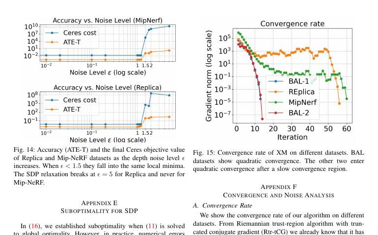
Fig. 14: Accuracy (ATE-T) and the final Ceres objective value of Replica and Mip-NeRF datasets as the depth noise level increases. When they fall into the same local minima. The SDP relaxation breaks at for Replica and never for Mip-NeRF.
图 14:Replica 与 Mip-NeRF 数据集上,随深度噪声水平升高的精度(ATE-T)与最终 Ceres 目标值。
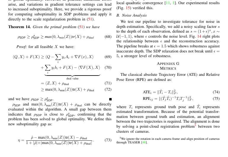
Fig. 15: Convergence rate of XM on different datasets. BAL datasets show quadratic convergence. The other two enter quadratic convergence after a slow convergence region.
图 15:XM 在不同数据集上的收敛速率。BAL 呈二次收敛;另外两个在缓慢阶段后进入二次收敛。
F-A Convergence Rate
F-A 收敛速率
We show the convergence rate of our algorithm on different datasets. From Riemannian trust-region algorithm with truncated conjugate gradient (Rtr-tCG) we already know that it has local quadratic convergence [11, 1]. Our experimental results (Fig. 15) verified this.
我们绘制不同数据集上目标值随迭代的下降曲线,观察二次收敛阶段。
F-B Noise Analysis
F-B 噪声分析
We test our pipeline to investigate tolerance for noise in depth estimation. Specifically, we add a noisy scaling factor to the depth of each observation, defined as , where controls the noise level. Fig. 14 right plots the relationship between and the reconstruction accuracy. The pipeline breaks at which shows robustness against inaccurate depth. The SDP relaxation does not break until , a stronger level of robustness.
在合成深度噪声下,ATE 与最终 Ceres 目标随噪声水平升高而变差;XM 热启动仍优于随机或弱初始化。
Appendix G Metrics
附录 G 度量
The classical absolute Trajectory Error (ATE) and Relative Pose Error (RPE) are defined as:
经典的绝对轨迹误差(ATE)与相对位姿误差(RPE)定义为:
where represents ground truth pose and represents estimated transformation. Because of the potential transformation between ground truth and estimation, an alignment between the two trajectories is required. The alignment is done by solving a point-cloud registration problem[^5] between two clusters of cameras.
ATE 衡量对齐后绝对轨迹误差,RPE 衡量相对位姿增量误差;两者均在适当相似变换对齐后计算。