Bottom-Up and Top-Down Attention for Image Captioning and Visual Question Answering
Bottom-Up and Top-Down Attention for Image Captioning and Visual Question Answering
自下而上与自上而下注意力:用于图像描述和视觉问答
Peter Anderson † † thanks: Work performed while interning at Microsoft. Xiaodong He Chris Buehler Affiliation: firstname.lastname@anu.edu.au, xiaodong.he@jd.com, {chris.buehler,leizhang}@microsoft.com Damien Teney Mark Johnson Affiliation: Australian National University JD AI Research Microsoft Research University of Adelaide Macquarie University Affiliation: damien.teney@adelaide.edu.au, mark.johnson@mq.edu.au Stephen Gould Lei Zhang Affiliation: Affiliation: firstname.lastname@anu.edu.au, xiaodong.he@jd.com, {chris.buehler,leizhang}@microsoft.com
Abstract
摘要
Top-down visual attention mechanisms have been used extensively in image captioning and visual question answering (VQA) to enable deeper image understanding through fine-grained analysis and even multiple steps of reasoning. In this work, we propose a combined bottom-up and top-down attention mechanism that enables attention to be calculated at the level of objects and other salient image regions. This is the natural basis for attention to be considered. Within our approach, the bottom-up mechanism (based on Faster R-CNN) proposes image regions, each with an associated feature vector, while the top-down mechanism determines feature weightings. Applying this approach to image captioning, our results on the MSCOCO test server establish a new state-of-the-art for the task, achieving CIDEr / SPICE / BLEU-4 scores of 117.9, 21.5 and 36.9, respectively. Demonstrating the broad applicability of the method, applying the same approach to VQA we obtain first place in the 2017 VQA Challenge.
自上而下的视觉注意力机制已广泛用于图像描述和视觉问答(VQA),以便通过细粒度分析、甚至多步推理来加深对图像的理解。本文提出一种自下而上与自上而下相结合的注意力机制,使注意力可以在物体及其他显著图像区域的层面上计算。这正是考虑注意力时更自然的基础。在我们的方法中,自下而上机制(基于 Faster R-CNN)提出图像区域,每个区域带有对应的特征向量,自上而下机制再决定这些特征的权重。把该方法用于图像描述时,我们在 MSCOCO 测试服务器上取得了当时该任务的最新结果,CIDEr / SPICE / BLEU-4 分别为 117.9、21.5 和 36.9。为说明方法的广泛适用性,我们把同一思路用于 VQA,并获得了 2017 年 VQA Challenge 第一名。
1 Introduction
1 引言
Problems combining image and language understanding such as image captioning [4] and visual question answering (VQA) [12] continue to inspire considerable research at the boundary of computer vision and natural language processing. In both these tasks it is often necessary to perform some fine-grained visual processing, or even multiple steps of reasoning to generate high quality outputs. As a result, visual attention mechanisms have been widely adopted in both image captioning [34, 27, 48, 46] and VQA [11, 28, 45, 47, 51]. These mechanisms improve performance by learning to focus on the regions of the image that are salient and are currently based on deep neural network architectures.
把图像理解与语言理解结合在一起的问题,例如图像描述 [4] 和视觉问答(VQA) [12],持续推动着计算机视觉与自然语言处理交界处的研究。这两类任务往往都需要进行一定的细粒度视觉处理,甚至多步推理,才能生成高质量输出。因此,视觉注意力机制已在图像描述 [34, 27, 48, 46] 和 VQA [11, 28, 45, 47, 51] 中被广泛采用。这些机制通过学习把焦点放在图像中显著的区域上来提升表现,目前均建立在深度神经网络架构之上。
In the human visual system, attention can be focused volitionally by top-down signals determined by the current task (e.g., looking for something), and automatically by bottom-up signals associated with unexpected, novel or salient stimuli [3, 6]. In this paper we adopt similar terminology and refer to attention mechanisms driven by non-visual or task-specific context as ‘top-down’, and purely visual feed-forward attention mechanisms as ‘bottom-up’.
在人类视觉系统中,注意力既可以在当前任务决定的自上而下信号驱动下有意识地聚焦(例如在寻找某件东西),也可以由与意外、新奇或显著刺激相关的自下而上信号自动引导 [3, 6]。本文沿用类似术语:把由非视觉或任务特定上下文驱动的注意力机制称为“自上而下”,把纯视觉前馈的注意力机制称为“自下而上”。
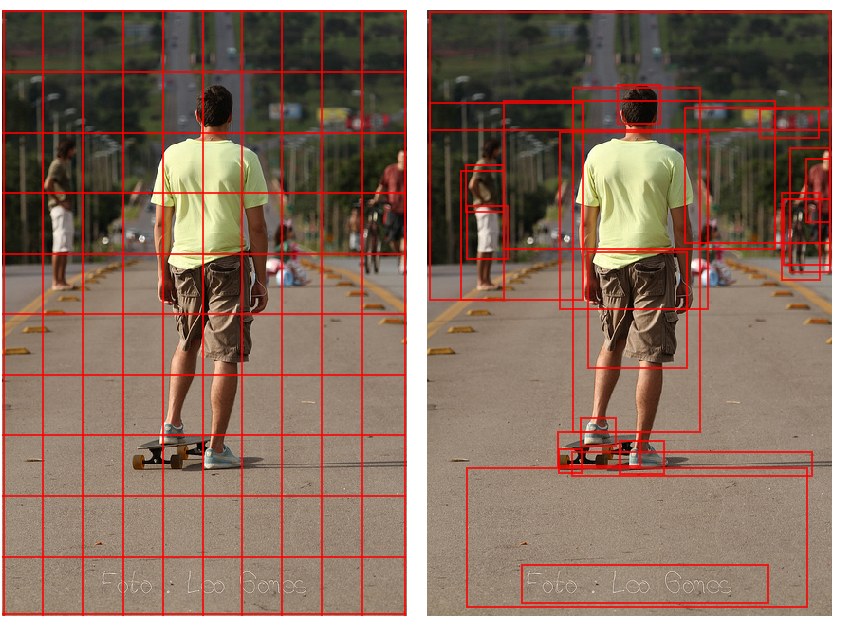
Figure 1: Typically, attention models operate on CNN features corresponding to a uniform grid of equally-sized image regions (left). Our approach enables attention to be calculated at the level of objects and other salient image regions (right).
图 1:通常,注意力模型作用在对应于均匀网格、大小相同的图像区域的 CNN 特征上(左)。我们的方法使注意力可以在物体及其他显著图像区域的层面上计算(右)。
Most conventional visual attention mechanisms used in image captioning and VQA are of the top-down variety. Taking as context a representation of a partially-completed caption output, or a question relating to the image, these mechanisms are typically trained to selectively attend to the output of one or more layers of a convolutional neural net (CNN). However, this approach gives little consideration to how the image regions that are subject to attention are determined. As illustrated conceptually in Figure 1, the resulting input regions correspond to a uniform grid of equally sized and shaped neural receptive fields – irrespective of the content of the image. To generate more human-like captions and question answers, objects and other salient image regions are a much more natural basis for attention [10, 36].
图像描述和 VQA 中常用的传统视觉注意力机制大多属于自上而下这一类。它们以部分已生成的描述,或与图像相关的问题作为上下文,通常被训练去选择性地关注卷积神经网络(CNN)一层或多层的输出。不过,这种方法很少考虑“被施加注意力的图像区域”本身是如何确定的。如图 1 概念所示,由此得到的输入区域对应于一组大小、形状都相同的神经感受野均匀网格——与图像内容无关。要生成更接近人类的描述和问答,物体及其他显著图像区域才是更自然的注意力基础 [10, 36]。
In this paper we propose a combined bottom-up and top-down visual attention mechanism. The bottom-up mechanism proposes a set of salient image regions, with each region represented by a pooled convolutional feature vector. Practically, we implement bottom-up attention using Faster R-CNN [33], which represents a natural expression of a bottom-up attention mechanism. The top-down mechanism uses task-specific context to predict an attention distribution over the image regions. The attended feature vector is then computed as a weighted average of image features over all regions.
本文提出一种自下而上与自上而下相结合的视觉注意力机制。自下而上机制提出一组显著图像区域,每个区域由池化后的卷积特征向量表示。实践中,我们用 Faster R-CNN [33] 实现自下而上注意力,它本身就是自下而上注意力机制的一种自然表达。自上而下机制利用任务特定上下文,预测这些图像区域上的注意力分布。加权平均所有区域的图像特征,就得到被关注的特征向量。
We evaluate the impact of combining bottom-up and top-down attention on two tasks. We first present an image captioning model that takes multiple glimpses of salient image regions during caption generation. Empirically, we find that the inclusion of bottom-up attention has a significant positive benefit for image captioning. Our results on the MSCOCO test server establish a new state-of-the-art for the task, achieving CIDEr / SPICE / BLEU-4 scores of 117.9, 21.5 and 36.9. respectively (outperforming all published and unpublished work at the time). Demonstrating the broad applicability of the method, we additionally present a VQA model using the same bottom-up attention features. Using this model we obtain first place in the 2017 VQA Challenge, achieving 70.3% overall accuracy on the VQA v2.0 test-standard server. Code, models and pre-computed image features are available from the project website[^1].
我们在两项任务上评估把自下而上与自上而下注意力结合起来的效果。首先给出一个图像描述模型,它在生成描述的过程中多次“瞥见”显著图像区域。实验表明,加入自下而上注意力对图像描述有明显的正向收益。我们在 MSCOCO 测试服务器上的结果刷新了该任务的最佳记录,CIDEr / SPICE / BLEU-4 分别为 117.9、21.5 和 36.9(当时超过了所有已发表和未发表的工作)。为说明方法的广泛适用性,我们另外给出一个使用同一套自下而上注意力特征的 VQA 模型。借助该模型,我们获得了 2017 年 VQA Challenge 第一名,在 VQA v2.0 test-standard 服务器上整体准确率为 70.3%。代码、模型以及预先计算的图像特征可在项目网站获取。[^1]
2 Related Work
2 相关工作
A large number of attention-based deep neural networks have been proposed for image captioning and VQA. Typically, these models can be characterized as top-down approaches, with context provided by a representation of a partially-completed caption in the case of image captioning [34, 27, 48, 46], or a representation of the question in the case of VQA [11, 28, 45, 47, 51]. In each case attention is applied to the output of one or more layers of a CNN, by predicting a weighting for each spatial location in the CNN output. However, determining the optimal number of image regions invariably requires an unwinnable trade-off between coarse and fine levels of detail. Furthermore, the arbitrary positioning of the regions with respect to image content may make it more difficult to detect objects that are poorly aligned to regions and to bind visual concepts associated with the same object.
已有大量基于注意力的深度网络被提出用于图像描述和 VQA。这些模型通常可概括为自上而下方法:在图像描述中,上下文来自部分已生成描述的表示 [34, 27, 48, 46];在 VQA 中,上下文来自问题的表示 [11, 28, 45, 47, 51]。无论哪种情形,注意力都作用在 CNN 一层或多层的输出上,具体做法是为 CNN 输出的每个空间位置预测一个权重。然而,要确定图像区域的最优数量,总是不得不在粗糙细节与精细细节之间做无法两全的折中。此外,这些区域相对于图像内容的位置是任意的,这可能使那些与区域对齐不佳的物体更难被检测,也更难把属于同一物体的视觉概念绑定在一起。
Comparatively few previous works have considered applying attention to salient image regions. We are aware of two papers. Jin et al. [18] use selective search [42] to identify salient image regions, which are filtered with a classifier then resized and CNN-encoded as input to an image captioning model with attention. The Areas of Attention captioning model [30] uses either edge boxes [52] or spatial transformer networks [17] to generate image features, which are processed using an attention model based on three bi-linear pairwise interactions [30]. In this work, rather than using hand-crafted or differentiable region proposals [42, 52, 17], we leverage Faster R-CNN [33], establishing a closer link between vision and language tasks and recent progress in object detection. With this approach we are able to pre-train our region proposals on object detection datasets. Conceptually, the advantages should be similar to pre-training visual representations on ImageNet [35] and leveraging significantly larger cross-domain knowledge. We additionally apply our method to VQA, establishing the broad applicability of our approach.
相对而言,此前很少有工作考虑把注意力施加在显著图像区域上。据我们所知有两篇。Jin 等人 [18] 用选择性搜索 [42] 找出显著图像区域,经分类器过滤后再缩放并由 CNN 编码,作为带注意力的图像描述模型的输入。Areas of Attention 描述模型 [30] 则用 edge boxes [52] 或空间变换网络 [17] 生成图像特征,再用基于三组双线性成对交互的注意力模型来处理 [30]。本文并不使用手工设计的或可微的区域提议 [42, 52, 17],而是借助 Faster R-CNN [33],从而在视觉–语言任务与目标检测的近期进展之间建立起更紧密的联系。这样,我们可以在目标检测数据集上预训练区域提议。从概念上看,其优势应类似于在 ImageNet [35] 上预训练视觉表示,并利用显著更大的跨领域知识。我们还把方法用到 VQA 上,以说明其广泛适用性。
3 Approach
3 方法
Given an image , both our image captioning model and our VQA model take as input a possibly variably-sized set of image features, , such that each image feature encodes a salient region of the image. The spatial image features can be variously defined as the output of our bottom-up attention model, or, following standard practice, as the spatial output layer of a CNN. We describe our approach to implementing a bottom-up attention model in Section 3.1. In Section 3.2 we outline the architecture of our image captioning model and in Section 3.3 we outline our VQA model. We note that for the top-down attention component, both models use simple one-pass attention mechanisms, as opposed to the more complex schemes of recent models such as stacked, multi-headed, or bidirectional attention [47, 16, 20, 28] that could also be applied.
给定图像 ,我们的图像描述模型和 VQA 模型都以一组数量可能不固定的 个图像特征作为输入,,使每个图像特征编码图像中的一个显著区域。空间图像特征 既可以定义成我们自下而上注意力模型的输出,也可以按常见做法定义成 CNN 的空间输出层。第 3.1 节介绍我们实现自下而上注意力模型的方法。第 3.2 节概述图像描述模型的架构,第 3.3 节概述 VQA 模型。需要指出的是,在自上而下注意力部分,两个模型都使用简单的单次注意力机制,而不是近期模型中更复杂的堆叠、多头或双向注意力方案 [47, 16, 20, 28];后者同样可以叠加使用。
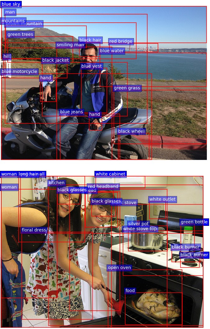
Figure 2: Example output from our Faster R-CNN bottom-up attention model. Each bounding box is labeled with an attribute class followed by an object class. Note however, that in captioning and VQA we utilize only the feature vectors – not the predicted labels.
图 2:我们基于 Faster R-CNN 的自下而上注意力模型的输出示例。每个边界框先标出属性类别,再标出物体类别。不过,在描述生成和 VQA 中我们只用特征向量,并不使用预测出的标签。
3.1 Bottom-Up Attention Model
3.1 自下而上注意力模型
The definition of spatial image features is generic. However, in this work we define spatial regions in terms of bounding boxes and implement bottom-up attention using Faster R-CNN [33]. Faster R-CNN is an object detection model designed to identify instances of objects belonging to certain classes and localize them with bounding boxes. Other region proposal networks could also be trained as an attentive mechanism [32, 25].
空间图像特征 的定义是通用的。但在本文中,我们用边界框来定义空间区域,并用 Faster R-CNN [33] 实现自下而上注意力。Faster R-CNN 是一种目标检测模型,用于识别属于特定类别的物体实例,并用边界框定位它们。其他区域提议网络也可以训练成一种注意力机制 [32, 25]。
Faster R-CNN detects objects in two stages. The first stage, described as a Region Proposal Network (RPN), predicts object proposals. A small network is slid over features at an intermediate level of a CNN. At each spatial location the network predicts a class-agnostic objectness score and a bounding box refinement for anchor boxes of multiple scales and aspect ratios. Using greedy non-maximum suppression with an intersection-over-union (IoU) threshold, the top box proposals are selected as input to the second stage. In the second stage, region of interest (RoI) pooling is used to extract a small feature map (e.g. ) for each box proposal. These feature maps are then batched together as input to the final layers of the CNN. The final output of the model consists of a softmax distribution over class labels and class-specific bounding box refinements for each box proposal.
Faster R-CNN 分两个阶段检测物体。第一阶段称为区域提议网络(RPN),用于预测物体提议。一个小型网络在 CNN 中间层特征上滑动。在每个空间位置,该网络为多种尺度和宽高比的锚框预测与类别无关的物体性分数以及边界框精修。再利用交并比(IoU)阈值做贪心非极大值抑制,选出排名靠前的框提议,作为第二阶段的输入。第二阶段用兴趣区域(RoI)池化,为每个框提议提取一小块特征图(例如 )。这些特征图再打包在一起,送入 CNN 的最后几层。模型的最终输出包括各类别标签上的 softmax 分布,以及每个框提议的类别相关边界框精修。
In this work, we use Faster R-CNN in conjunction with the ResNet-101 [13] CNN. To generate an output set of image features for use in image captioning or VQA, we take the final output of the model and perform non-maximum suppression for each object class using an IoU threshold. We then select all regions where any class detection probability exceeds a confidence threshold. For each selected region , is defined as the mean-pooled convolutional feature from this region, such that the dimension of the image feature vectors is 2048. Used in this fashion, Faster R-CNN effectively functions as a ‘hard’ attention mechanism, as only a relatively small number of image bounding box features are selected from a large number of possible configurations.
本文把 Faster R-CNN 与 ResNet-101 [13] CNN 结合使用。为了给图像描述或 VQA 生成一组输出图像特征 ,我们取模型的最终输出,并按每个物体类别、使用一个 IoU 阈值做非极大值抑制。然后选出任一类别检测概率超过置信度阈值的全部区域。对每个被选中的区域 , 定义为该区域的均值池化卷积特征,从而使图像特征向量的维数 为 2048。按这种方式使用时,Faster R-CNN 实际上起到一种“硬”注意力机制的作用,因为只从大量可能的配置中选出相对较少的图像边界框特征。
To pretrain the bottom-up attention model, we first initialize Faster R-CNN with ResNet-101 pretrained for classification on ImageNet [35]. We then train on Visual Genome [21] data. To aid the learning of good feature representations, we add an additional training output for predicting attribute classes (in addition to object classes). To predict attributes for region , we concatenate the mean pooled convolutional feature with a learned embedding of the ground-truth object class, and feed this into an additional output layer defining a softmax distribution over each attribute class plus a ‘no attributes’ class.
为预训练自下而上注意力模型,我们首先用在 ImageNet [35] 上做分类预训练的 ResNet-101 初始化 Faster R-CNN,再在 Visual Genome [21] 数据上训练。为帮助学到更好的特征表示,我们额外增加一个训练输出,用于预测属性类别(作为物体类别之外的补充)。要预测区域 的属性,我们将均值池化卷积特征 与真实物体类别的可学习嵌入拼接,再送入一个额外的输出层,该层在每个属性类别以及一个“无属性”类别上定义 softmax 分布。
The original Faster R-CNN multi-task loss function contains four components, defined over the classification and bounding box regression outputs for both the RPN and the final object class proposals respectively. We retain these components and add an additional multi-class loss component to train the attribute predictor. In Figure 2 we provide some examples of model output.
原先的 Faster R-CNN 多任务损失函数包含四个部分,分别定义在 RPN 以及最终物体类别提议的分类输出和边界框回归输出上。我们保留这些部分,并再增加一个多类损失项来训练属性预测器。图 2 给出了一些模型输出示例。
3.2 Captioning Model
3.2 描述生成模型
Given a set of image features , our proposed captioning model uses a ‘soft’ top-down attention mechanism to weight each feature during caption generation, using the existing partial output sequence as context. This approach is broadly similar to several previous works [34, 27, 46]. However, the particular design choices outlined below make for a relatively simple yet high-performing baseline model. Even without bottom-up attention, our captioning model achieves performance comparable to state-of-the-art on most evaluation metrics (refer Table 1).
给定一组图像特征 ,我们提出的描述生成模型在生成描述时使用“软”的自上而下注意力机制,为每个特征加权,并以已有的部分输出序列作为上下文。这一思路与若干已有工作大体相似 [34, 27, 46]。不过,下面列出的具体设计选择,使它成为一个相对简单却表现很好的基线模型。即便不加自下而上注意力,我们的描述生成模型在大多数评价指标上也已能与当时的领先水平相当(见表 1)。
At a high level, the captioning model is composed of two LSTM [15] layers using a standard implementation [9]. In the sections that follow we will refer to the operation of the LSTM over a single time step using the following notation:
从整体上看,描述生成模型由两个采用标准实现 [9] 的 LSTM [15] 层组成。后文中,我们用如下记号表示 LSTM 在单个时间步上的运算:
where is the LSTM input vector and is the LSTM output vector. Here we have neglected the propagation of memory cells for notational convenience. We now describe the formulation of the LSTM input vector and the output vector for each layer of the model. The overall captioning model is illustrated in Figure 3.
其中 是 LSTM 的输入向量, 是 LSTM 的输出向量。为书写方便,这里略去了记忆单元的传递。下面分别说明模型每一层中 LSTM 输入向量 与输出向量 的构成。完整的描述生成模型如图 3 所示。
3.2.1 Top-Down Attention LSTM
Within the captioning model, we characterize the first LSTM layer as a top-down visual attention model, and the second LSTM layer as a language model, indicating each layer with superscripts in the equations that follow. Note that the bottom-up attention model is described in Section 3.1, and in this section its outputs are simply considered as features . The input vector to the attention LSTM at each time step consists of the previous output of the language LSTM, concatenated with the mean-pooled image feature and an encoding of the previously generated word, given by:
3.2.1 自上而下注意力 LSTM
在描述生成模型中,我们把第一层 LSTM 视为自上而下的视觉注意力模型,把第二层 LSTM 视为语言模型,并在随后的公式中用上标区分各层。需要注意,自下而上注意力模型已在第 3.1 节介绍,本节只把它的输出当作特征 。注意力 LSTM 在每个时间步的输入向量,由语言模型 LSTM 的上一时刻输出、均值池化图像特征 ,以及前一个已生成词的编码拼接而成,即:
where is a word embedding matrix for a vocabulary , and is one-hot encoding of the input word at timestep . These inputs provide the attention LSTM with maximum context regarding the state of the language LSTM, the overall content of the image, and the partial caption output generated so far, respectively. The word embedding is learned from random initialization without pretraining.
其中 是词表 上的词嵌入矩阵, 是时间步 输入词的 one-hot 编码。这些输入分别向注意力 LSTM 提供关于语言 LSTM 状态、整幅图像整体内容,以及目前已生成的部分描述的最大上下文。词嵌入从随机初始化开始学习,不做预训练。
Given the output of the attention LSTM, at each time step we generate a normalized attention weight for each of the image features as follows:
给定注意力 LSTM 的输出 ,我们在每个时间步 为 个图像特征 中的每一个生成归一化注意力权重 ,如下:
where , and are learned parameters. The attended image feature used as input to the language LSTM is calculated as a convex combination of all input features:
其中 、 和 是可学习参数。送入语言 LSTM 的被关注图像特征,按所有输入特征的凸组合计算:
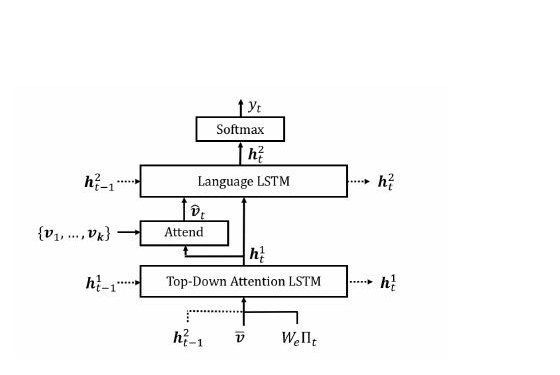
Figure 3: Overview of the proposed captioning model. Two LSTM layers are used to selectively attend to spatial image features . These features can be defined as the spatial output of a CNN, or following our approach, generated using bottom-up attention.
图 3:所提出描述生成模型的概览。两个 LSTM 层用于选择性地关注空间图像特征 。这些特征可以定义成 CNN 的空间输出,也可以按我们的方法,用自下而上注意力生成。
3.2.2 Language LSTM
The input to the language model LSTM consists of the attended image feature, concatenated with the output of the attention LSTM, given by:
3.2.2 语言 LSTM
语言模型 LSTM 的输入由被关注的图像特征与注意力 LSTM 的输出拼接而成,即:
Using the notation to refer to a sequence of words , at each time step the conditional distribution over possible output words is given by:
用记号 表示词序列 ,则在每个时间步 ,可能输出词上的条件分布为:
where and are learned weights and biases. The distribution over complete output sequences is calculated as the product of conditional distributions:
其中 和 是可学习的权重和偏置。完整输出序列上的分布由各条件分布的乘积得到:
3.2.3 Objective
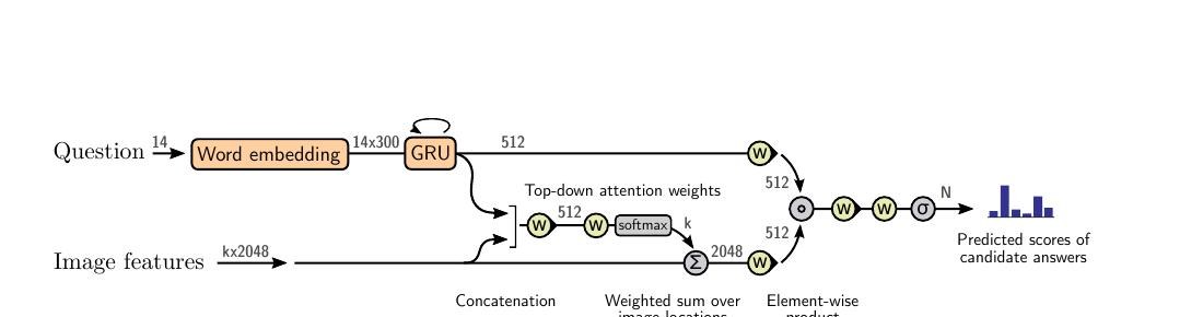
Figure 4: Overview of the proposed VQA model. A deep neural network implements a joint embedding of the question and image features . These features can be defined as the spatial output of a CNN, or following our approach, generated using bottom-up attention. Output is generated by a multi-label classifier operating over a fixed set of candidate answers. Gray numbers indicate the dimensions of the vector representations between layers. Yellow elements use learned parameters.
3.2.3 训练目标
图 4:所提出 VQA 模型的概览。一个深度神经网络实现问题与图像特征 的联合嵌入。这些特征可以定义成 CNN 的空间输出,也可以按我们的方法,用自下而上注意力生成。输出由一个在固定候选答案集合上工作的多标签分类器产生。灰色数字表示各层之间向量表示的维数。黄色模块使用可学习参数。
Given a target ground truth sequence and a captioning model with parameters , we minimize the following cross entropy loss:
给定目标真实序列 以及参数为 的描述生成模型,我们最小化如下交叉熵损失:
For fair comparison with recent work [34] we also report results optimized for CIDEr [43]. Initializing from the cross-entropy trained model, we seek to minimize the negative expected score:
为了与近期工作 [34] 公平比较,我们也报告针对 CIDEr [43] 优化的结果。从交叉熵训练得到的模型出发,我们希望最小化负的期望分数:
where is the score function (e.g., CIDEr). Following the approach described as Self-Critical Sequence Training [34] (SCST), the gradient of this loss can be approximated:
其中 是评分函数(例如 CIDEr)。按照称为 Self-Critical Sequence Training [34](SCST)的方法,该损失的梯度可以近似为:
where is a sampled caption and defines the baseline score obtained by greedily decoding the current model. SCST (like other REINFORCE [44] algorithms) explores the space of captions by sampling from the policy during training. This gradient tends to increase the probability of sampled captions that score higher than the score from the current model.
其中 是采样得到的描述, 表示用当前模型做贪心解码得到的基线分数。SCST(与其他 REINFORCE [44] 算法一样)在训练时通过从策略中采样来探索描述空间。这一梯度倾向于提高那些得分高于当前模型得分的采样描述的概率。
In our experiments, we follow SCST but we speed up the training process by restricting the sampling distribution. Using beam search decoding, we sample only from those captions in the decoded beam. Empirically, we have observed when decoding using beam search that the resulting beam typically contains at least one very high scoring caption – although frequently this caption does not have the highest log-probability of the set. In contrast, we observe that very few unrestricted caption samples score higher than the greedily-decoded caption. Using this approach, we complete CIDEr optimization in a single epoch.
在实验中我们沿用 SCST,但通过限制采样分布来加快训练。使用束搜索解码时,我们只从解码束中的那些描述里采样。经验上我们观察到:用束搜索解码时,得到的束里通常至少包含一条分数很高的描述——尽管这条描述常常并不是集合中对数概率最高的那一条。相比之下,几乎没有不受限采样得到的描述能超过贪心解码描述的分数。用这种方法,我们在单个周期内就完成了 CIDEr 优化。
3.3 VQA Model
3.3 视觉问答模型
Given a set of spatial image features , our proposed VQA model also uses a ‘soft’ top-down attention mechanism to weight each feature, using the question representation as context. As illustrated in Figure 4, the proposed model implements the well-known joint multimodal embedding of the question and the image, followed by a prediction of regression of scores over a set of candidate answers. This approach has been the basis of numerous previous models [16, 20, 39]. However, as with our captioning model, implementation decisions are important to ensure that this relatively simple model delivers high performance.
给定一组空间图像特征 ,我们提出的 VQA 模型同样使用“软”的自上而下注意力机制为每个特征加权,并以问题表示作为上下文。如图 4 所示,该模型实现了问题和图像的经典联合多模态嵌入,随后在一组候选答案上做分数回归预测。这一思路是众多已有模型的基础 [16, 20, 39]。不过,与描述生成模型一样,具体实现选择对于确保这个相对简单的模型仍能取得高表现十分重要。
The learned non-linear transformations within the network are implemented with gated hyperbolic tangent activations [7]. These are a special case of highway networks [37] that have shown a strong empirical advantage over traditional ReLU or tanh layers. Each of our ‘gated tanh’ layers implements a function with parameters defined as follows:
网络中的可学习非线性变换用门控双曲正切激活实现 [7]。它们是高速网络 [37] 的一种特例,经验上相对传统的 ReLU 或 tanh 层有明显优势。我们的每一个“门控 tanh”层实现函数 ,参数为 ,定义如下:
where is the sigmoid activation function, are learned weights, are learned biases, and is the Hadamard (element-wise) product. The vector acts multiplicatively as a gate on the intermediate activation .
其中 是 sigmoid 激活函数, 是可学习权重, 是可学习偏置, 是 Hadamard(逐元素)积。向量 以乘法方式作为中间激活 上的门。
Our proposed approach first encodes each question as the hidden state of a gated recurrent unit [5] (GRU), with each input word represented using a learned word embedding. Similar to Equation 3, given the output of the GRU, we generate an unnormalized attention weight for each of the image features as follows:
我们的方法首先把每个问题编码为门控循环单元 [5](GRU)的隐状态 ,其中每个输入词用可学习的词嵌入表示。与公式 3 类似,给定 GRU 的输出 ,我们为 个图像特征 中的每一个生成未归一化的注意力权重 ,如下:
where is a learned parameter vector. Equation 4 and Equation 5 (neglecting subscripts ) are used to calculate the normalized attention weight and the attended image feature . The distribution over possible output responses is given by:
其中 是可学习参数向量。公式 4 和公式 5(略去下标 )用于计算归一化注意力权重以及被关注的图像特征 。可能输出回答 上的分布由下式给出:
Where is a joint representation of the question and the image, and are learned weights.
其中 是问题与图像的联合表示, 是可学习权重。
Due to space constraints, some important aspects of our VQA approach are not detailed here. For full specifics of the VQA model including a detailed exploration of architectures and hyperparameters, refer to Teney et al. [38].
受篇幅所限,我们 VQA 方法中的一些重要细节未在此展开。关于 VQA 模型的完整说明,包括对架构和超参数的详细探讨,请参见 Teney 等人 [38]。
4 Evaluation
4 实验评估
| Cross-Entropy Loss | CIDEr Optimization | ||||||||||||
|---|---|---|---|---|---|---|---|---|---|---|---|---|---|
| BLEU-1 | BLEU-4 | METEOR | ROUGE-L | CIDEr | SPICE | BLEU-1 | BLEU-4 | METEOR | ROUGE-L | CIDEr | SPICE | ||
| SCST:Att2in [34] | - | 31.3 | 26.0 | 54.3 | 101.3 | - | - | 33.3 | 26.3 | 55.3 | 111.4 | - | |
| SCST:Att2all [34] | - | 30.0 | 25.9 | 53.4 | 99.4 | - | - | 34.2 | 26.7 | 55.7 | 114.0 | - | |
| Ours: ResNet | 74.5 | 33.4 | 26.1 | 54.4 | 105.4 | 19.2 | 76.6 | 34.0 | 26.5 | 54.9 | 111.1 | 20.2 | |
| Ours: Up-Down | 77.2 | 36.2 | 27.0 | 56.4 | 113.5 | 20.3 | 79.8 | 36.3 | 27.7 | 56.9 | 120.1 | 21.4 | |
| Relative Improvement | 4% | 8% | 3% | 4% | 8% | 6% | 4% | 7% | 5% | 4% | 8% | 6% |
Table 1: Single-model image captioning performance on the MSCOCO Karpathy test split. Our baseline ResNet model obtains similar results to SCST [34], the existing state-of-the-art on this test set. Illustrating the contribution of bottom-up attention, our Up-Down model achieves significant (3–8%) relative gains across all metrics regardless of whether cross-entropy loss or CIDEr optimization is used.
| 交叉熵损失 | CIDEr 优化 | ||||||||||||
|---|---|---|---|---|---|---|---|---|---|---|---|---|---|
| BLEU-1 | BLEU-4 | METEOR | ROUGE-L | CIDEr | SPICE | BLEU-1 | BLEU-4 | METEOR | ROUGE-L | CIDEr | SPICE | ||
| SCST:Att2in [34] | - | 31.3 | 26.0 | 54.3 | 101.3 | - | - | 33.3 | 26.3 | 55.3 | 111.4 | - | |
| SCST:Att2all [34] | - | 30.0 | 25.9 | 53.4 | 99.4 | - | - | 34.2 | 26.7 | 55.7 | 114.0 | - | |
| Ours: ResNet | 74.5 | 33.4 | 26.1 | 54.4 | 105.4 | 19.2 | 76.6 | 34.0 | 26.5 | 54.9 | 111.1 | 20.2 | |
| Ours: Up-Down | 77.2 | 36.2 | 27.0 | 56.4 | 113.5 | 20.3 | 79.8 | 36.3 | 27.7 | 56.9 | 120.1 | 21.4 | |
| 相对提升 | 4% | 8% | 3% | 4% | 8% | 6% | 4% | 7% | 5% | 4% | 8% | 6% |
表 1:在 MSCOCO Karpathy 测试划分上的单模型图像描述表现。我们的 ResNet 基线与该测试集上当时的领先方法 SCST [34] 结果相近。为说明自下而上注意力的贡献,无论使用交叉熵损失还是 CIDEr 优化,我们的 Up-Down 模型在所有指标上都取得了显著的相对提升(3%–8%)。
| Cross-Entropy Loss | CIDEr Optimization | ||||||||||||||
|---|---|---|---|---|---|---|---|---|---|---|---|---|---|---|---|
| SPICE | Objects | Attributes | Relations | Color | Count | Size | SPICE | Objects | Attributes | Relations | Color | Count | Size | ||
| Ours: ResNet | 19.2 | 35.4 | 8.6 | 5.3 | 12.2 | 4.1 | 3.9 | 20.2 | 37.0 | 9.2 | 6.1 | 10.6 | 12.0 | 4.3 | |
| Ours: Up-Down | 20.3 | 37.1 | 9.2 | 5.8 | 12.7 | 6.5 | 4.5 | 21.4 | 39.1 | 10.0 | 6.5 | 11.4 | 18.4 | 3.2 |
Table 2: Breakdown of SPICE F-scores over various subcategories on the MSCOCO Karpathy test split. Our Up-Down model outperforms the ResNet baseline at identifying objects, as well as detecting object attributes and the relations between objects.
| 交叉熵损失 | CIDEr 优化 | ||||||||||||||
|---|---|---|---|---|---|---|---|---|---|---|---|---|---|---|---|
| SPICE | 物体 | 属性 | 关系 | 颜色 | 数量 | 尺寸 | SPICE | 物体 | 属性 | 关系 | 颜色 | 数量 | 尺寸 | ||
| Ours: ResNet | 19.2 | 35.4 | 8.6 | 5.3 | 12.2 | 4.1 | 3.9 | 20.2 | 37.0 | 9.2 | 6.1 | 10.6 | 12.0 | 4.3 | |
| Ours: Up-Down | 20.3 | 37.1 | 9.2 | 5.8 | 12.7 | 6.5 | 4.5 | 21.4 | 39.1 | 10.0 | 6.5 | 11.4 | 18.4 | 3.2 |
表 2:在 MSCOCO Karpathy 测试划分上,SPICE F 分数按若干子类别的分解。我们的 Up-Down 模型在识别物体、检测物体属性以及物体之间的关系上都优于 ResNet 基线。
4.1 Datasets
4.1 数据集
4.1.1 Visual Genome Dataset
We use the Visual Genome [21] dataset to pretrain our bottom-up attention model, and for data augmentation when training our VQA model. The dataset contains 108K images densely annotated with scene graphs containing objects, attributes and relationships, as well as 1.7M visual question answers.
4.1.1 Visual Genome 数据集
我们用 Visual Genome [21] 数据集预训练自下而上注意力模型,并在训练 VQA 模型时做数据增强。该数据集包含 10.8 万张图像,带有包含物体、属性和关系的稠密场景图标注,以及 170 万条视觉问答。
For pretraining the bottom-up attention model, we use only the object and attribute data. We reserve 5K images for validation, and 5K images for future testing, treating the remaining 98K images as training data. As approximately 51K Visual Genome images are also found in the MSCOCO captions dataset [23], we are careful to avoid contamination of our MSCOCO validation and test sets. We ensure that any images found in both datasets are contained in the same split in both datasets.
预训练自下而上注意力模型时,我们只使用物体和属性数据。我们留出 5 千张图像做验证、5 千张图像留作将来测试,将其余 9.8 万张图像作为训练数据。由于大约 5.1 万张 Visual Genome 图像也出现在 MSCOCO 描述数据集 [23] 中,我们小心避免污染自己的 MSCOCO 验证集和测试集:凡是同时出现在两个数据集中的图像,都会被放进两个数据集里相同的划分。
As the object and attribute annotations consist of freely annotated strings, rather than classes, we perform extensive cleaning and filtering of the training data. Starting from 2,000 object classes and 500 attribute classes, we manually remove abstract classes that exhibit poor detection performance in initial experiments. Our final training set contains 1,600 object classes and 400 attribute classes. Note that we do not merge or remove overlapping classes (e.g. ‘person’, ‘man’, ‘guy’), classes with both singular and plural versions (e.g. ‘tree’, ‘trees’) and classes that are difficult to precisely localize (e.g. ‘sky’, ‘grass’, ‘buildings’).
由于物体和属性标注是自由书写的字符串而不是类别,我们对训练数据做了充分的清理和过滤。从 2000 个物体类别和 500 个属性类别出发,我们手工去掉了在初步实验中检测表现较差的抽象类别。最终训练集包含 1600 个物体类别和 400 个属性类别。需要说明的是,我们没有合并或删除重叠类别(例如 “person”“man”“guy”)、同时具有单数和复数形式的类别(例如 “tree”“trees”),以及难以精确定位的类别(例如 “sky”“grass”“buildings”)。
When training the VQA model, we augment the VQA v2.0 training data with Visual Genome question and answer pairs provided the correct answer is present in model’s answer vocabulary. This represents about 30% of the available data, or 485K questions.
训练 VQA 模型时,我们在 VQA v2.0 训练数据之外,加入正确答案出现在模型答案词表中的 Visual Genome 问答对。这大约占可用数据的 30%,即 48.5 万个问题。
4.1.2 Microsoft COCO Dataset
To evaluate our proposed captioning model, we use the MSCOCO 2014 captions dataset [23]. For validation of model hyperparameters and offline testing, we use the ‘Karpathy’ splits [19] that have been used extensively for reporting results in prior work. This split contains 113,287 training images with five captions each, and 5K images respectively for validation and testing. Our MSCOCO test server submission is trained on the entire MSCOCO 2014 training and validation set (123K images).
4.1.2 Microsoft COCO 数据集
为评估所提出的描述生成模型,我们使用 MSCOCO 2014 描述数据集 [23]。超参数验证和离线测试采用此前工作中广泛使用的 “Karpathy” 划分 [19]。该划分包含 113,287 张训练图像(每张五条描述),验证和测试各 5 千张图像。提交到 MSCOCO 测试服务器的模型在整个 MSCOCO 2014 训练加验证集(12.3 万张图像)上训练。
We follow standard practice and perform only minimal text pre-processing, converting all sentences to lower case, tokenizing on white space, and filtering words that do not occur at least five times, resulting in a model vocabulary of 10,010 words. To evaluate caption quality, we use the standard automatic evaluation metrics, namely SPICE [1], CIDEr [43], METEOR [8], ROUGE-L [22] and BLEU [29].
我们按惯例只做最少的文本预处理:把所有句子转为小写,按空白分词,并过滤出现次数少于五次的词,最终模型词表大小为 10,010。评估描述质量时,我们使用标准自动评价指标,即 SPICE [1]、CIDEr [43]、METEOR [8]、ROUGE-L [22] 和 BLEU [29]。
4.1.3 VQA v2.0 Dataset
To evaluate our proposed VQA model, we use the recently introduced VQA v2.0 dataset [12], which attempts to minimize the effectiveness of learning dataset priors by balancing the answers to each question. The dataset, which was used as the basis of the 2017 VQA Challenge[^2], contains 1.1M questions with 11.1M answers relating to MSCOCO images.
4.1.3 VQA v2.0 数据集
为评估所提出的 VQA 模型,我们使用当时新发布的 VQA v2.0 数据集 [12]。该数据集通过对每个问题的答案做平衡,试图降低学习数据集先验的有效性。它被用作 2017 年 VQA Challenge 的基础[^2],包含与 MSCOCO 图像相关的 110 万个问题和 1110 万条答案。
We perform standard question text preprocessing and tokenization. Questions are trimmed to a maximum of 14 words for computational efficiency. The set of candidate answers is restricted to correct answers in the training set that appear more than 8 times, resulting in an output vocabulary size of 3,129. Our VQA test server submissions are trained on the training and validation sets plus additional questions and answers from Visual Genome. To evaluate answer quality, we report accuracies using the standard VQA metric [2], which takes into account the occasional disagreement between annotators for the ground truth answers.
我们对问题文本做标准预处理和分词。为降低计算开销,问题被截断到最多 14 个词。候选答案集合限制为训练集中出现超过 8 次的正确答案,输出词表大小为 3,129。提交到 VQA 测试服务器的模型在训练集和验证集上训练,并额外使用来自 Visual Genome 的问答。评估答案质量时,我们用标准 VQA 指标 [2] 报告准确率,该指标会考虑标注者在真实答案上偶尔出现的不一致。
| BLEU-1 | BLEU-2 | BLEU-3 | BLEU-4 | METEOR | ROUGE-L | CIDEr | SPICE | ||||||||||||||||
|---|---|---|---|---|---|---|---|---|---|---|---|---|---|---|---|---|---|---|---|---|---|---|---|
| c5 | c40 | c5 | c40 | c5 | c40 | c5 | c40 | c5 | c40 | c5 | c40 | c5 | c40 | c5 | c40 | ||||||||
| Review Net [48] | 72.0 | 90.0 | 55.0 | 81.2 | 41.4 | 70.5 | 31.3 | 59.7 | 25.6 | 34.7 | 53.3 | 68.6 | 96.5 | 96.9 | 18.5 | 64.9 | |||||||
| Adaptive [27] | 74.8 | 92.0 | 58.4 | 84.5 | 44.4 | 74.4 | 33.6 | 63.7 | 26.4 | 35.9 | 55.0 | 70.5 | 104.2 | 105.9 | 19.7 | 67.3 | |||||||
| PG-BCMR [24] | 75.4 | - | 59.1 | - | 44.5 | - | 33.2 | - | 25.7 | - | 55 | - | 101.3 | - | - | - | |||||||
| SCST:Att2all [34] | 78.1 | 93.7 | 61.9 | 86.0 | 47.0 | 75.9 | 35.2 | 64.5 | 27.0 | 35.5 | 56.3 | 70.7 | 114.7 | 116.7 | 20.7 | 68.9 | |||||||
| LSTM-A [49] | 78.7 | 93.7 | 62.7 | 86.7 | 47.6 | 76.5 | 35.6 | 65.2 | 27 | 35.4 | 56.4 | 70.5 | 116 | 118 | - | - | |||||||
| Ours: Up-Down | 80.2 | 95.2 | 64.1 | 88.8 | 49.1 | 79.4 | 36.9 | 68.5 | 27.6 | 36.7 | 57.1 | 72.4 | 117.9 | 120.5 | 21.5 | 71.5 |
Table 3: Highest ranking published image captioning results on the online MSCOCO test server. Our submission, an ensemble of 4 models optimized for CIDEr with different initializations, outperforms previously published work on all reported metrics. At the time of submission (18 July 2017), we also outperformed all unpublished test server submissions.
| 方法 | BLEU-1 c5 | BLEU-1 c40 | BLEU-2 c5 | BLEU-2 c40 | BLEU-3 c5 | BLEU-3 c40 | BLEU-4 c5 | BLEU-4 c40 | METEOR c5 | METEOR c40 | ROUGE-L c5 | ROUGE-L c40 | CIDEr c5 | CIDEr c40 | SPICE c5 | SPICE c40 |
|---|---|---|---|---|---|---|---|---|---|---|---|---|---|---|---|---|
| Review Net [48] | 72.0 | 90.0 | 55.0 | 81.2 | 41.4 | 70.5 | 31.3 | 59.7 | 25.6 | 34.7 | 53.3 | 68.6 | 96.5 | 96.9 | 18.5 | 64.9 |
| Adaptive [27] | 74.8 | 92.0 | 58.4 | 84.5 | 44.4 | 74.4 | 33.6 | 63.7 | 26.4 | 35.9 | 55.0 | 70.5 | 104.2 | 105.9 | 19.7 | 67.3 |
| PG-BCMR [24] | 75.4 | - | 59.1 | - | 44.5 | - | 33.2 | - | 25.7 | - | 55 | - | 101.3 | - | - | - |
| SCST:Att2all [34] | 78.1 | 93.7 | 61.9 | 86.0 | 47.0 | 75.9 | 35.2 | 64.5 | 27.0 | 35.5 | 56.3 | 70.7 | 114.7 | 116.7 | 20.7 | 68.9 |
| LSTM-A [49] | 78.7 | 93.7 | 62.7 | 86.7 | 47.6 | 76.5 | 35.6 | 65.2 | 27 | 35.4 | 56.4 | 70.5 | 116 | 118 | - | - |
| Ours: Up-Down | 80.2 | 95.2 | 64.1 | 88.8 | 49.1 | 79.4 | 36.9 | 68.5 | 27.6 | 36.7 | 57.1 | 72.4 | 117.9 | 120.5 | 21.5 | 71.5 |
表 3:在线 MSCOCO 测试服务器上排名最高的已发表图像描述结果。我们的提交是 4 个以不同初始化、针对 CIDEr 优化的模型的集成,在全部报告指标上都超过了此前已发表的工作。在提交时(2017 年 7 月 18 日),我们也超过了测试服务器上所有未发表的提交。
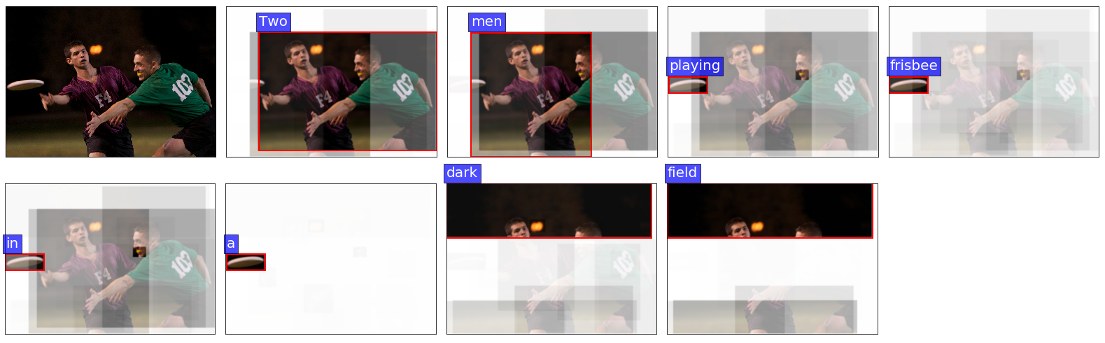
Two men playing frisbee in a dark field.
Figure 5: Example of a generated caption showing attended image regions. For each generated word, we visualize the attention weights on individual pixels, outlining the region with the maximum attention weight in red. Avoiding the conventional trade-off between coarse and fine levels of detail, our model focuses on both closely-cropped details, such as the frisbee and the green player’s mouthguard when generating the word ‘playing’, as well as large regions, such as the night sky when generating the word ‘dark’.
两名男子在黑暗的场地里玩飞盘。
图 5:一条生成描述及其关注图像区域的示例。对每个生成的词,我们可视化各个像素上的注意力权重,并用红色标出注意力权重最大的区域。我们的模型不必在粗糙细节与精细细节之间做传统折中:生成 “playing” 一词时,它可以聚焦被紧密裁切的细节,例如飞盘和绿衣选手的护齿;生成 “dark” 一词时,它又可以关注较大的区域,例如夜空。
4.2 ResNet Baseline
4.2 ResNet 基线
To quantify the impact of bottom-up attention, in both our captioning and VQA experiments we evaluate our full model (Up-Down) against prior work as well as an ablated baseline. In each case, the baseline (ResNet), uses a ResNet [13] CNN pretrained on ImageNet [35] to encode each image in place of the bottom-up attention mechanism.
为量化自下而上注意力的作用,我们在描述生成和 VQA 实验中,都把完整模型(Up-Down)与已有工作以及一个消融基线相比较。两种情形下,基线(ResNet)都用在 ImageNet [35] 上预训练的 ResNet [13] CNN 来编码每张图像,以代替自下而上注意力机制。
In image captioning experiments, similarly to previous work [34] we encode the full-sized input image with the final convolutional layer of Resnet-101, and use bilinear interpolation to resize the output to a fixed size spatial representation of 1010. This is equivalent to the maximum number of spatial regions used in our full model. In VQA experiments, we encode the resized input image with ResNet-200 [14]. In separate experiments we use evaluate the effect of varying the size of the spatial output from its original size of 1414, to 77 (using bilinear interpolation) and 11 (i.e., mean pooling without attention).
在图像描述实验中,与已有工作 [34] 类似,我们用 ResNet-101 的最后一层卷积编码全尺寸输入图像,再用双线性插值把输出调整到固定大小的 空间表示。这与完整模型使用的空间区域数上限相当。在 VQA 实验中,我们用 ResNet-200 [14] 编码调整尺寸后的输入图像。在另外的实验中,我们评估了把空间输出从原来的 变为 (用双线性插值)以及 (即不做注意力的均值池化)的影响。
4.3 Image Captioning Results
4.3 图像描述结果
In Table 1 we report the performance of our full model and the ResNet baseline in comparison to the existing state-of-the-art Self-critical Sequence Training [34] (SCST) approach on the test portion of the Karpathy splits. For fair comparison, results are reported for models trained with both standard cross-entropy loss, and models optimized for CIDEr score. Note that the SCST approach uses ResNet-101 encoding of full images, similar to our ResNet baseline. All results are reported for a single model with no fine-tuning of the input ResNet / R-CNN model. However, the SCST results are selected from the best of four random initializations, while our results are outcomes from a single initialization.
表 1 报告了我们的完整模型和 ResNet 基线,在 Karpathy 划分测试部分上,相对于当时领先的 Self-critical Sequence Training [34](SCST)方法的表现。为公平比较,我们同时报告用标准交叉熵损失训练的模型,以及针对 CIDEr 分数优化的模型。需要说明的是,SCST 方法用 ResNet-101 编码整幅图像,与我们的 ResNet 基线类似。全部结果均为单个模型、且不对输入的 ResNet / R-CNN 模型做微调。不过,SCST 的结果选自四次随机初始化中最好的一次,而我们的结果来自单次初始化。
Relative to the SCST models, our ResNet baseline obtains slightly better performance under cross-entropy loss, and slightly worse performance when optimized for CIDEr score. After incorporating bottom-up attention, our full Up-Down model shows significant improvements across all metrics regardless of whether cross-entropy loss or CIDEr optimization is used. Using just a single model, we obtain the best reported results for the Karpathy test split. As illustrated in Table 2, the contribution from bottom-up attention is broadly based, illustrated by improved performance in terms of identifying objects, object attributes and also the relationships between objects.
相对于 SCST 模型,我们的 ResNet 基线在交叉熵损失下略好,在针对 CIDEr 分数优化时略差。加入自下而上注意力后,无论使用交叉熵损失还是 CIDEr 优化,完整的 Up-Down 模型在所有指标上都有显著提升。仅用单个模型,我们就取得了 Karpathy 测试划分上当时最好的报告结果。如表 2 所示,自下而上注意力的贡献较为全面,体现在识别物体、检测物体属性以及物体之间关系等方面的提升。
Table 3 reports the performance of 4 ensembled models trained with CIDEr optimization on the official MSCOCO evaluation server, along with the highest ranking previously published results. At the time of submission (18 July 2017), we outperform all other test server submissions on all reported evaluation metrics.
表 3 报告了 4 个针对 CIDEr 优化的集成模型在官方 MSCOCO 评测服务器上的表现,并与当时排名最高的已发表结果对照。在提交时(2017 年 7 月 18 日),我们在全部报告的评价指标上都超过了测试服务器上的其他提交。
4.4 VQA Results
4.4 视觉问答结果
| Yes/No | Number | Other | Overall | ||
|---|---|---|---|---|---|
| Ours: ResNet (11) | 76.0 | 36.5 | 46.8 | 56.3 | |
| Ours: ResNet (1414) | 76.6 | 36.2 | 49.5 | 57.9 | |
| Ours: ResNet (77) | 77.6 | 37.7 | 51.5 | 59.4 | |
| Ours: Up-Down | 80.3 | 42.8 | 55.8 | 63.2 | |
| Relative Improvement | 3% | 14% | 8% | 6% |
Table 4: Single-model performance on the VQA v2.0 validation set. The use of bottom-up attention in the Up-Down model provides a significant improvement over the best ResNet baseline across all question types, even though the ResNet baselines use almost twice as many convolutional layers.
| 是/否 | 计数 | 其他 | 总体 | ||
|---|---|---|---|---|---|
| Ours: ResNet (11) | 76.0 | 36.5 | 46.8 | 56.3 | |
| Ours: ResNet (1414) | 76.6 | 36.2 | 49.5 | 57.9 | |
| Ours: ResNet (77) | 77.6 | 37.7 | 51.5 | 59.4 | |
| Ours: Up-Down | 80.3 | 42.8 | 55.8 | 63.2 | |
| 相对提升 | 3% | 14% | 8% | 6% |
表 4:VQA v2.0 验证集上的单模型表现。尽管 ResNet 基线使用了几乎两倍的卷积层,Up-Down 模型中的自下而上注意力仍在所有问题类型上相对最好的 ResNet 基线带来了显著提升。
| Yes/No | Number | Other | Overall | ||
|---|---|---|---|---|---|
| Prior [12] | 61.20 | 0.36 | 1.17 | 25.98 | |
| Language-only [12] | 67.01 | 31.55 | 27.37 | 44.26 | |
| d-LSTM+n-I [26, 12] | 73.46 | 35.18 | 41.83 | 54.22 | |
| MCB [11, 12] | 78.82 | 38.28 | 53.36 | 62.27 | |
| UPMC-LIP6 | 82.07 | 41.06 | 57.12 | 65.71 | |
| Athena | 82.50 | 44.19 | 59.97 | 67.59 | |
| HDU-USYD-UNCC | 84.50 | 45.39 | 59.01 | 68.09 | |
| Ours: Up-Down | 86.60 | 48.64 | 61.15 | 70.34 |
Table 5: VQA v2.0 test-standard server accuracy as at 8 August 2017, ranking our submission against published and unpublished work for each question type. Our approach, an ensemble of 30 models, outperforms all other leaderboard entries.
| 是/否 | 计数 | 其他 | 总体 | ||
|---|---|---|---|---|---|
| Prior [12] | 61.20 | 0.36 | 1.17 | 25.98 | |
| Language-only [12] | 67.01 | 31.55 | 27.37 | 44.26 | |
| d-LSTM+n-I [26, 12] | 73.46 | 35.18 | 41.83 | 54.22 | |
| MCB [11, 12] | 78.82 | 38.28 | 53.36 | 62.27 | |
| UPMC-LIP6 | 82.07 | 41.06 | 57.12 | 65.71 | |
| Athena | 82.50 | 44.19 | 59.97 | 67.59 | |
| HDU-USYD-UNCC | 84.50 | 45.39 | 59.01 | 68.09 | |
| Ours: Up-Down | 86.60 | 48.64 | 61.15 | 70.34 |
表 5:截至 2017 年 8 月 8 日,VQA v2.0 test-standard 服务器准确率,按问题类型将我们的提交与已发表和未发表工作对照。我们的方法是 30 个模型的集成,超过了排行榜上的所有其他条目。
In Table 4 we report the single model performance of our full Up-Down VQA model relative to several ResNet baselines on the VQA v2.0 validation set. The addition of bottom-up attention provides a significant improvement over the best ResNet baseline across all question types, even though the ResNet baseline uses approximately twice as many convolutional layers. Table 5 reports the performance of 30 ensembled models on the official VQA 2.0 test-standard evaluation server, along with the previously published baseline results and the highest ranking other entries. At the time of submission (8 August 2017), we outperform all other test server submissions. Our submission also achieved first place in the 2017 VQA Challenge.
表 4 报告了完整 Up-Down VQA 模型相对于若干 ResNet 基线,在 VQA v2.0 验证集上的单模型表现。加入自下而上注意力后,尽管 ResNet 基线使用了大约两倍的卷积层,完整模型仍在所有问题类型上相对最好的 ResNet 基线有显著提升。表 5 报告了 30 个集成模型在官方 VQA 2.0 test-standard 评测服务器上的表现,并对照此前已发表的基线结果以及排名最高的其他条目。在提交时(2017 年 8 月 8 日),我们超过了测试服务器上的所有其他提交。该提交还获得了 2017 年 VQA Challenge 第一名。
4.5 Qualitative Analysis
4.5 定性分析
To help qualitatively evaluate our attention methodology, in Figure 5 we visualize the attended image regions for different words generated by our Up-Down captioning model. As indicated by this example, our approach is equally capable of focusing on fine details or large image regions. This capability arises because the attention candidates in our model consist of many overlapping regions with varying scales and aspect ratios – each aligned to an object, several related objects, or an otherwise salient image patch.
为从定性上评估我们的注意力方法,图 5 可视化了 Up-Down 描述生成模型在生成不同词时所关注的图像区域。这一示例表明,我们的方法既能聚焦细小细节,也能关注较大的图像区域。这种能力来自:模型中的注意力候选由许多尺度和宽高比各不相同、彼此重叠的区域组成——每一个都对齐到一个物体、若干相关物体,或其他显著的图像块。
Unlike conventional approaches, when a candidate attention region corresponds to an object, or several related objects, all the visual concepts associated with those objects appear to be spatially co-located – and are processed together. In other words, our approach is able to consider all of the information pertaining to an object at once. This is also a natural way for attention to be implemented. In the human visual system, the problem of integrating the separate features of objects in the correct combinations is known as the feature binding problem, and experiments suggest that attention plays a central role in the solution [41, 40]. We include an example of VQA attention in Figure 6.
与传统方法不同,当候选注意力区域对应于一个物体或若干相关物体时,与这些物体相关的全部视觉概念在空间上似乎是共置的,并被一并处理。换句话说,我们的方法能够一次性考虑与某个物体有关的全部信息。这也是实现注意力的一种自然方式。在人类视觉系统中,如何把物体的各个分离特征以正确组合整合起来,被称为特征绑定问题;实验表明注意力在其解决中起着核心作用 [41, 40]。图 6 给出了一个 VQA 注意力的例子。
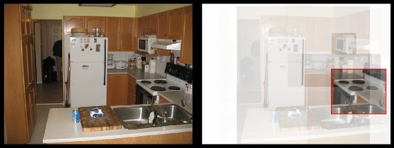
Question: What room are they in? Answer: kitchen
Figure 6: VQA example illustrating attention output. Given the question ‘What room are they in?’, the model focuses on the stovetop, generating the answer ‘kitchen’.
问题:他们在哪个房间?答案:厨房
图 6:展示注意力输出的 VQA 示例。面对问题 “What room are they in?”,模型聚焦在炉灶上,并生成答案 “kitchen”。
5 Conclusion
5 结论
We present a novel combined bottom-up and top-down visual attention mechanism. Our approach enables attention to be calculated more naturally at the level of objects and other salient regions. Applying this approach to image captioning and visual question answering, we achieve state-of-the-art results in both tasks, while improving the interpretability of the resulting attention weights.
我们提出一种新颖的自下而上与自上而下相结合的视觉注意力机制。该方法使注意力可以更自然地在物体及其他显著区域的层面上计算。把它用于图像描述和视觉问答,我们在两项任务上都取得了当时的领先结果,同时提高了所得注意力权重的可解释性。
At a high level, our work more closely unifies tasks involving visual and linguistic understanding with recent progress in object detection. While this suggests several directions for future research, the immediate benefits of our approach may be captured by simply replacing pretrained CNN features with pretrained bottom-up attention features.
从更高层面看,这项工作把涉及视觉与语言理解的任务,与目标检测的近期进展更紧密地统一起来。这提示了若干未来研究方向;而该方法的直接收益,或许只需用预训练的自下而上注意力特征替换预训练的 CNN 特征就能获得。
Acknowledgements
致谢
This research is partially supported by an Australian Government Research Training Program (RTP) Scholarship, by the Australian Research Council Centre of Excellence for Robotic Vision (project number CE140100016), by a Google award through the Natural Language Understanding Focused Program, and under the Australian Research Council’s Discovery Projects funding scheme (project number DP160102156).
本研究部分得到澳大利亚政府研究培训计划(RTP)奖学金、澳大利亚研究理事会机器人视觉卓越中心(项目号 CE140100016)、谷歌通过 Natural Language Understanding Focused Program 提供的奖励,以及澳大利亚研究理事会 Discovery Projects 资助计划(项目号 DP160102156)的支持。
References
参考文献
[1] P. Anderson, B. Fernando, M. Johnson, and S. Gould. SPICE: Semantic propositional image caption evaluation. In ECCV , 2016.
[2] S. Antol, A. Agrawal, J. Lu, M. Mitchell, D. Batra, C. L. Zitnick, and D. Parikh. VQA: Visual Question Answering. In ICCV , 2015.
[3] T. J. Buschman and E. K. Miller. Top-down versus bottom-up control of attention in the prefrontal and posterior parietal cortices. Science , 315(5820):1860–1862, 2007.
[4] X. Chen, T.-Y. L. Hao Fang, R. Vedantam, S. Gupta, P. Dollar, and C. L. Zitnick. Microsoft COCO captions: Data collection and evaluation server. arXiv preprint arXiv:1504.00325 , 2015.
[5] K. Cho, B. van Merrienboer, C. Gulcehre, F. Bougares, H. Schwenk, and Y. Bengio. Learning phrase representations using RNN encoder-decoder for statistical machine translation. In EMNLP , 2014.
[6] M. Corbetta and G. L. Shulman. Control of goal-directed and stimulus-driven attention in the brain. Nature Reviews Neuroscience , 3(3):201–215, 2002.
[7] Y. N. Dauphin, A. Fan, M. Auli, and D. Grangier. Language modeling with gated convolutional networks. arXiv preprint arXiv:1612.08083 , 2016.
[8] M. Denkowski and A. Lavie. Meteor Universal: Language Specific Translation Evaluation for Any Target Language. In Proceedings of the EACL 2014 Workshop on Statistical Machine Translation , 2014.
[9] J. Donahue, L. A. Hendricks, S. Guadarrama, M. Rohrbach, S. Venugopalan, K. Saenko, and T. Darrell. Long-term recurrent convolutional networks for visual recognition and description. In CVPR , 2015.
[10] R. Egly, J. Driver, and R. D. Rafal. Shifting visual attention between objects and locations: evidence from normal and parietal lesion subjects. Journal of Experimental Psychology: General , 123(2):161, 1994.
[11] A. Fukui, D. H. Park, D. Yang, A. Rohrbach, T. Darrell, and M. Rohrbach. Multimodal compact bilinear pooling for visual question answering and visual grounding. In EMNLP , 2016.
[12] Y. Goyal, T. Khot, D. Summers-Stay, D. Batra, and D. Parikh. Making the V in VQA matter: Elevating the role of image understanding in Visual Question Answering. In CVPR , 2017.
[13] K. He, X. Zhang, S. Ren, and J. Sun. Deep residual learning for image recognition. In CVPR , 2016.
[14] K. He, X. Zhang, S. Ren, and J. Sun. Identity mappings in deep residual networks. arXiv preprint arXiv:1603.05027 , 2016.
[15] S. Hochreiter and J. Schmidhuber. Long short-term memory. Neural Computation , 1997.
[16] A. Jabri, A. Joulin, and L. van der Maaten. Revisiting visual question answering baselines. arXiv preprint arXiv:1606.08390 , 2016.
[17] M. Jaderberg, K. Simonyan, A. Zisserman, and K. Kavukcuoglu. Spatial transformer networks. In NIPS , 2015.
[18] J. Jin, K. Fu, R. Cui, F. Sha, and C. Zhang. Aligning where to see and what to tell: image caption with region-based attention and scene factorization. arXiv preprint arXiv:1506.06272 , 2015.
[19] A. Karpathy and F.-F. Li. Deep visual-semantic alignments for generating image descriptions. In CVPR , 2015.
[20] V. Kazemi and A. Elqursh. Show, ask, attend, and answer: A strong baseline for visual question answering. arXiv preprint arXiv:1704.03162 , 2017.
[21] R. Krishna, Y. Zhu, O. Groth, J. Johnson, K. Hata, J. Kravitz, S. Chen, Y. Kalantidis, L.-J. Li, D. A. Shamma, M. Bernstein, and L. Fei-Fei. Visual genome: Connecting language and vision using crowdsourced dense image annotations. arXiv preprint arXiv:1602.07332 , 2016.
[22] C. Lin. Rouge: a package for automatic evaluation of summaries. In ACL Workshop , 2004.
[23] T. Lin, M. Maire, S. Belongie, J. Hays, P. Perona, D. Ramanan, P. Dollar, and C. L. Zitnick. Microsoft COCO: Common objects in context. In ECCV , 2014.
[24] S. Liu, Z. Zhu, N. Ye, S. Guadarrama, and K. Murphy. Improved image captioning via policy gradient optimization of spider. In ICCV , 2017.
[25] W. Liu, D. Anguelov, D. Erhan, C. Szegedy, S. Reed, C.-Y. Fu, and A. C. Berg. SSD: Single shot multibox detector. arXiv preprint arXiv:1512.02325 , 2015.
[26] J. Lu, X. Lin, D. Batra, and D. Parikh. Deeper lstm and normalized cnn visual question answering model. https://github.com/VT-vision-lab/VQA_LSTM_CNN , 2015.
[27] J. Lu, C. Xiong, D. Parikh, and R. Socher. Knowing when to look: Adaptive attention via a visual sentinel for image captioning. In CVPR , 2017.
[28] J. Lu, J. Yang, D. Batra, and D. Parikh. Hierarchical question-image co-attention for visual question answering. In NIPS , 2016.
[29] K. Papineni, S. Roukos, T. Ward, and W. Zhu. Bleu: a method for automatic evaluation of machine translation. In ACL , 2002.
[30] M. Pedersoli, T. Lucas, C. Schmid, and J. Verbeek. Areas of attention for image captioning. In ICCV , 2017.
[31] J. Pennington, R. Socher, and C. D. Manning. GloVe: Global Vectors for Word Representation. In Proceedings of the Conference on Empirical Methods for Natural Language Processing (EMNLP) , 2014.
[32] J. Redmon, S. K. Divvala, R. B. Girshick, and A. Farhadi. You only look once: Unified, real-time object detection. In CVPR , 2016.
[33] S. Ren, K. He, R. Girshick, and J. Sun. Faster R-CNN: Towards real-time object detection with region proposal networks. In NIPS , 2015.
[34] S. J. Rennie, E. Marcheret, Y. Mroueh, J. Ross, and V. Goel. Self-critical sequence training for image captioning. In CVPR , 2017.
[35] O. Russakovsky, J. Deng, H. Su, J. Krause, S. Satheesh, S. Ma, Z. Huang, A. Karpathy, A. Khosla, M. Bernstein, A. C. Berg, and L. Fei-Fei. Imagenet large scale visual recognition challenge. IJCV , 2015.
[36] B. J. Scholl. Objects and attention: The state of the art. Cognition , 80(1):1–46, 2001.
[37] R. K. Srivastava, K. Greff, and J. Schmidhuber. Highway networks. arXiv preprint arXiv:1505.00387v1 , 2015.
[38] D. Teney, P. Anderson, X. He, and A. van den Hengel. Tips and tricks for visual question answering: Learnings from the 2017 challenge. In CVPR , 2018.
[39] D. Teney and A. van den Hengel. Zero-shot visual question answering. arXiv preprint arXiv:1611.05546 , 2016.
[40] A. Treisman. Perceptual grouping and attention in visual search for features and for objects. Journal of Experimental Psychology: Human Perception and Performance , 8(2):194, 1982.
[41] A. M. Treisman and G. Gelade. A feature-integration theory of attention. Cognitive Psychology , 12:97–136, 1980.
[42] J. R. Uijlings, K. E. Van De Sande, T. Gevers, and A. W. Smeulders. Selective search for object recognition. IJCV , 2013.
[43] R. Vedantam, C. L. Zitnick, and D. Parikh. CIDEr: Consensus-based image description evaluation. In CVPR , 2015.
[44] R. J. Williams. Simple statistical gradient-following algorithms for connectionist reinforcement learning. Mach. Learn. , 8(3-4):229–256, May 1992.
[45] H. Xu and K. Saenko. Ask, attend and answer: Exploring question-guided spatial attention for visual question answering. In ECCV , 2016.
[46] K. Xu, J. Ba, R. Kiros, K. Cho, A. C. Courville, R. Salakhutdinov, R. S. Zemel, and Y. Bengio. Show, attend and tell: Neural image caption generation with visual attention. In ICML , 2015.
[47] Z. Yang, X. He, J. Gao, L. Deng, and A. J. Smola. Stacked attention networks for image question answering. In CVPR , 2016.
[48] Z. Yang, Y. Yuan, Y. Wu, R. Salakhutdinov, and W. W. Cohen. Review networks for caption generation. In NIPS , 2016.
[49] T. Yao, Y. Pan, Y. Li, Z. Qiu, and T. Mei. Boosting image captioning with attributes. In ICCV , 2017.
[50] M. D. Zeiler. ADADELTA: an adaptive learning rate method. arXiv preprint arXiv:1212.5701 , 2012.
[51] Y. Zhu, O. Groth, M. Bernstein, and L. Fei-Fei. Visual7w: Grounded question answering in images. In CVPR , 2016.
[52] L. Zitnick and P. Dollár. Edge boxes: Locating object proposals from edges. In ECCV , 2014.
SUPPLEMENTARY MATERIALS
补充材料
6 Implementation Details
6 实现细节
6.1 Bottom-Up Attention Model
6.1 自下而上注意力模型
Our bottom-up attention Faster R-CNN implementation uses an IoU threshold of 0.7 for region proposal suppression, and 0.3 for object class suppression. To select salient image regions, a class detection confidence threshold of 0.2 is used, allowing the number of regions per image to vary with the complexity of the image, up to a maximum of 100. However, in initial experiments we find that simply selecting the top 36 features in each image works almost as well in both downstream tasks. Since Visual Genome [21] contains a relatively large number of annotations per image, the model is relatively intensive to train. Using 8 Nvidia M40 GPUs, we take around 5 days to complete 380K training iterations, although we suspect that faster training regimes could also be effective.
我们的自下而上注意力 Faster R-CNN 实现中,区域提议抑制的 IoU 阈值为 0.7,物体类别抑制的 IoU 阈值为 0.3。选择显著图像区域时,类别检测置信度阈值为 0.2,从而每张图像的区域数 可以随图像复杂度变化,最多为 100。不过,在初步实验中我们发现,简单地在每张图像中选取排名最高的 36 个特征,在两个下游任务上几乎同样有效。由于 Visual Genome [21] 每张图像的标注数量较多,模型训练相对耗时。使用 8 块 Nvidia M40 GPU,我们大约用 5 天完成 38 万次训练迭代,尽管我们猜想更快的训练安排也可能有效。
6.2 Captioning Model
6.2 描述生成模型
In the captioning model, we set the number of hidden units in each LSTM to 1,000, the number of hidden units in the attention layer to 512, and the size of the input word embedding to 1,000. In training, we use a simple learning rate schedule, beginning with a learning rate of 0.01 which is reduced to zero on a straight-line basis over 60K iterations using a batch size of 100 and a momentum parameter of 0.9. Training using two Nvidia Titan X GPUs takes around 9 hours (including less than one hour for CIDEr optimization). During optimization and decoding we use a beam size of 5. When decoding we also enforce the constraint that a single word cannot be predicted twice in a row. Note that in both our captioning and VQA models, image features are fixed and not finetuned.
在描述生成模型中,我们把每个 LSTM 的隐单元数 设为 1000,注意力层的隐单元数 设为 512,输入词嵌入大小 设为 1000。训练时我们使用简单的学习率安排:初始学习率为 0.01,并在 6 万次迭代中按直线降到零,批次大小为 100,动量参数为 0.9。用两块 Nvidia Titan X GPU 训练大约需要 9 小时(其中 CIDEr 优化不到 1 小时)。优化和解码时束大小为 5。解码时我们还施加约束:同一个词不能被连续预测两次。需要说明的是,在描述生成和 VQA 模型中,图像特征都是固定的,不做微调。
6.3 VQA Model
6.3 视觉问答模型
In the VQA model, we use 300 dimension word embeddings, initialized with pretrained GloVe vectors [31], and we use hidden states of dimension 512. We train the VQA model using AdaDelta [50] and regularize with early stopping. The training of the model takes in the order of 12–18 hours on a single Nvidia K40 GPU. Refer to Teney et al. [38] for further details of the VQA model implementation.
在 VQA 模型中,我们使用 300 维词嵌入,并用预训练的 GloVe 向量 [31] 初始化,隐状态维数为 512。我们用 AdaDelta [50] 训练 VQA 模型,并用早停做正则。模型训练在单块 Nvidia K40 GPU 上大约需要 12 到 18 小时。更多 VQA 模型实现细节见 Teney 等人 [38]。
7 Additional Examples
7 更多示例
In Figure 7 we qualitatively compare attention methodologies for image caption generation, by illustrating attention weights for the ResNet baseline and our full Up-Down model on the same image. The baseline ResNet model hallucinates a toilet and therefore generates a poor quality caption. In contrast, our Up-Down model correctly identifies the couch, despite the novel scene composition. Additional examples of generated captions can be found in Figures 8 and 9. Additional visual question answering examples can be found in Figures 10 and 11.
图 7 从定性上比较不同注意力方法在图像描述生成中的差异:我们在同一张图像上展示 ResNet 基线和完整 Up-Down 模型的注意力权重。基线 ResNet 模型幻想出了一个马桶,因而生成了质量较差的描述。相比之下,尽管场景组合少见,我们的 Up-Down 模型仍正确识别出了沙发。更多生成描述的示例见图 8 和图 9。更多视觉问答示例如图 10 和图 11。
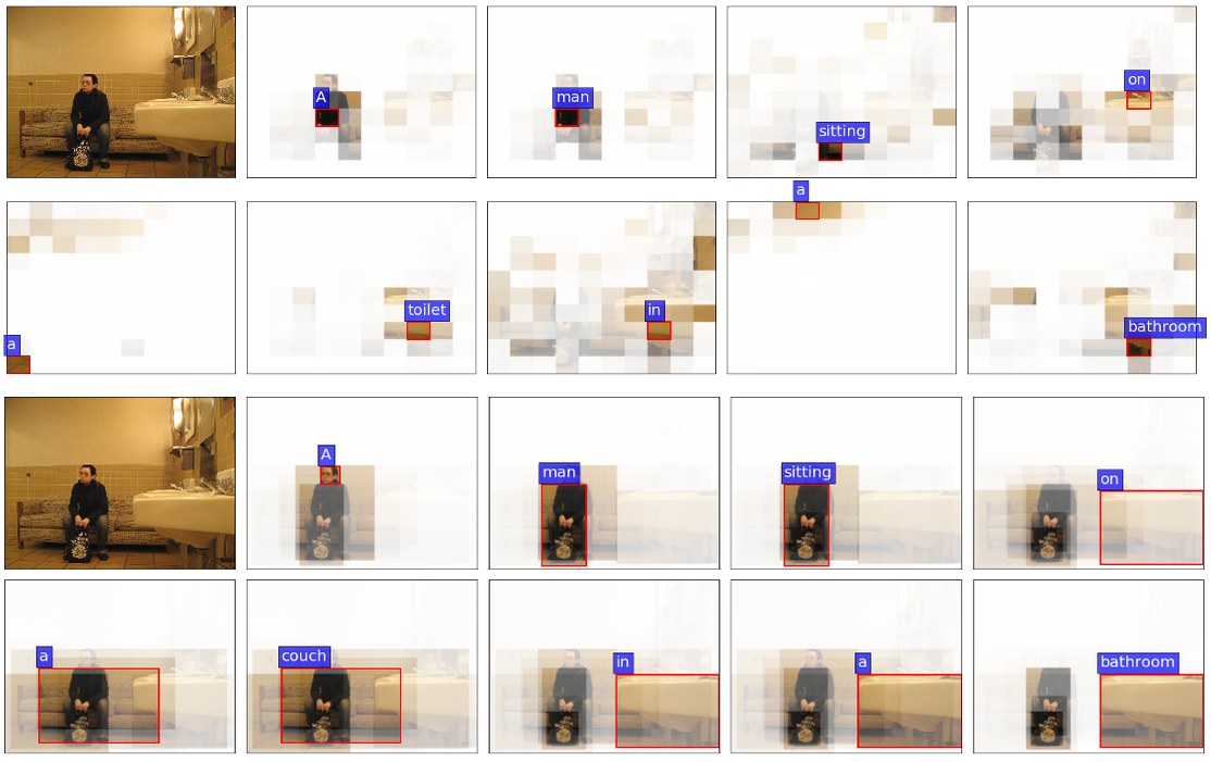
Resnet – A man sitting on a toilet in a bathroom.
Up-Down – A man sitting on a couch in a bathroom.
Figure 7: Qualitative differences between attention methodologies in caption generation. For each generated word, we visualize the attended image region, outlining the region with the maximum attention weight in red. The selected image is unusual because it depicts a bathroom containing a couch but no toilet. Nevertheless, our baseline ResNet model (top) hallucinates a toilet, presumably from language priors, and therefore generates a poor quality caption. In contrast, our Up-Down model (bottom) clearly identifies the out-of-context couch, generating a correct caption while also providing more interpretable attention weights.
Resnet —— 一个男人坐在浴室里的马桶上。
Up-Down —— 一个男人坐在浴室里的沙发上。
图 7:描述生成中不同注意力方法的定性差异。对每个生成的词,我们可视化被关注的图像区域,并用红色标出注意力权重最大的区域。所选图像较为少见,因为它描绘的是一间有沙发、却没有马桶的浴室。尽管如此,我们的基线 ResNet 模型(上)仍幻想出一个马桶,这大概来自语言先验,因而生成了质量较差的描述。相比之下,我们的 Up-Down 模型(下)清楚地识别出了这一脱离语境的沙发,生成了正确的描述,同时提供了更可解释的注意力权重。
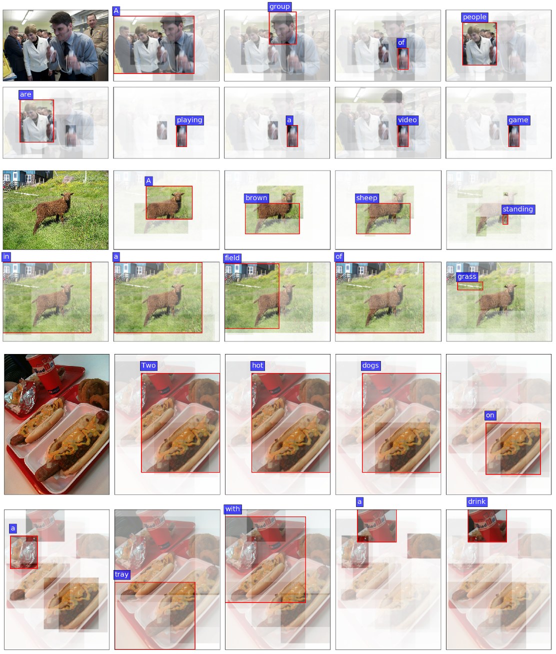
A group of people are playing a video game.
A brown sheep standing in a field of grass.
Two hot dogs on a tray with a drink.
Figure 8: Examples of generated captions showing attended image regions. Attention is given to fine details, such as: (1) the man’s hands holding the game controllers in the top image, and (2) the sheep’s legs when generating the word ‘standing’ in the middle image. Our approach can avoid the trade-off between coarse and fine levels of detail.
一群人正在玩电子游戏。
一只棕色的羊站在草地上。
托盘上有两份热狗,旁边有一杯饮料。
图 8:展示被关注图像区域的生成描述示例。注意力会落到细小细节上,例如:(1)上图中男人握着游戏手柄的手;(2)中间图像在生成 “standing” 一词时关注到羊的腿。我们的方法可以避免在粗糙细节与精细细节之间做折中。
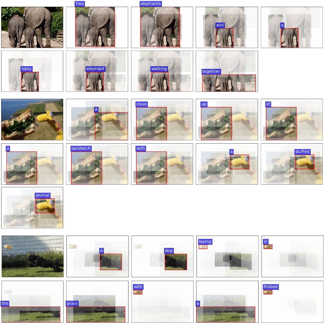
Two elephants and a baby elephant walking together.
A close up of a sandwich with a stuffed animal.
A dog laying in the grass with a frisbee.
Figure 9: Further examples of generated captions showing attended image regions. The first example suggests an understanding of spatial relationships when generating the word ‘together’. The middle image demonstrates the successful captioning of a compositionally novel scene. The bottom example is a failure case. The dog’s pose is mistaken for laying, rather than jumping – possibly due to poor salient region cropping that misses the dog’s head and feet.
两头大象和一头小象一起走。
一份三明治的特写,旁边有一只毛绒玩具。
一只狗躺在草地上,旁边有一个飞盘。
图 9:更多展示被关注图像区域的生成描述示例。第一个例子在生成 “together” 一词时,显示出对空间关系的理解。中间图像表明模型能够成功描述组合上新奇的场景。底部是一个失败例子:狗的姿势被误认成躺着,而不是跳跃——这可能是因为显著区域裁切不佳,漏掉了狗的头和脚。
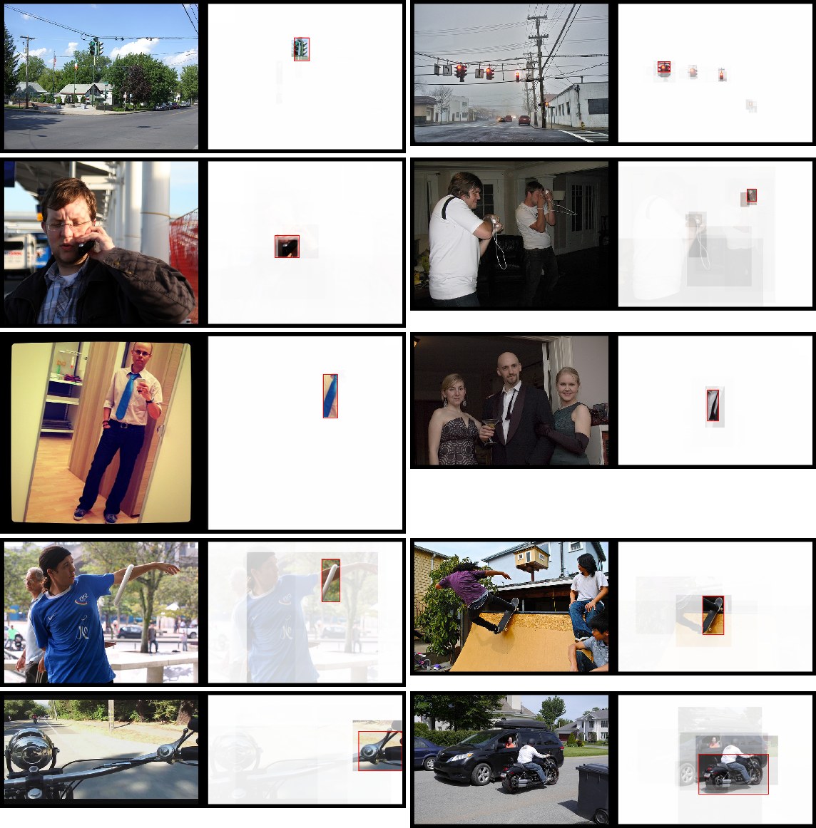
Question: What color is illuminated on the traffic light? Answer left: green. Answer right: red. Question: What is the man holding? Answer left: phone. Answer right: controller. Question: What color is his tie? Answer left: blue. Answer right: black. Question: What sport is shown? Answer left: frisbee. Answer right: skateboarding. Question: Is this the handlebar of a motorcycle? Answer left: yes. Answer right: no.
Figure 10: Further examples of successful visual question answering results, showing attended image regions.
问题:交通灯亮的是什么颜色?左图答案:绿色。右图答案:红色。问题:这个男人拿着什么?左图答案:手机。右图答案:手柄。问题:他的领带是什么颜色?左图答案:蓝色。右图答案:黑色。问题:图中是什么运动?左图答案:飞盘。右图答案:滑板。问题:这是摩托车的车把吗?左图答案:是。右图答案:否。
图 10:更多成功的视觉问答结果示例,并展示被关注的图像区域。
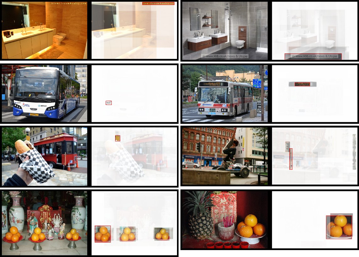
Question: What is the name of the realty company? Answer left: none. Answer right: none. Question: What is the bus number? Answer left: 2. Answer right: 23. Question: How many cones have reflective tape? Answer left: 2. Answer right: 1. Question: How many oranges are on pedestals? Answer left: 2. Answer right: 2.
Figure 11: Examples of visual question answering (VQA) failure cases. Although our simple VQA model has limited reading and counting capabilities, the attention maps are often correctly focused.
问题:这家房地产公司叫什么名字?左图答案:无。右图答案:无。问题:公交车号码是多少?左图答案:2。右图答案:23。问题:有多少个锥桶带有反光带?左图答案:2。右图答案:1。问题:底座上有多少个橙子?左图答案:2。右图答案:2。
图 11:视觉问答(VQA)失败例子。尽管我们这个简单的 VQA 模型在阅读和计数方面能力有限,注意力图却常常正确地聚焦。