Bi-Directional Attention Flow for Machine Comprehension

面向机器阅读理解的双向注意力流

Minjoon Seo † † thanks: The majority of the work was done while the author was interning at the Allen Institute for AI.    Aniruddha Kembhavi    Ali Farhadi    Hananneh Hajishirzi    University of Washington    Allen Institute for Artificial Intelligence {minjoon,ali,hannaneh}@cs.washington.edu , {anik}@allenai.org

Abstract

摘要

Machine comprehension (MC), answering a query about a given context paragraph, requires modeling complex interactions between the context and the query. Recently, attention mechanisms have been successfully extended to MC. Typically these methods use attention to focus on a small portion of the context and summarize it with a fixed-size vector, couple attentions temporally, and/or often form a uni-directional attention. In this paper we introduce the Bi-Directional Attention Flow (BiDAF) network, a multi-stage hierarchical process that represents the context at different levels of granularity and uses bi-directional attention flow mechanism to obtain a query-aware context representation without early summarization. Our experimental evaluations show that our model achieves the state-of-the-art results in Stanford Question Answering Dataset (SQuAD) and CNN/DailyMail cloze test.

机器阅读理解（MC）要回答关于一段给定上下文的问题，需要把上下文与问题之间的复杂交互建出来。近年来，注意力机制已被成功地推广到阅读理解。这些方法通常用注意力聚焦上下文中的一小部分，并把它收成一个固定长度的向量，把注意力在时间上耦合起来，并且往往只做单方向注意。本文引入双向注意力流（BiDAF）网络：这是一个分多阶段的层次化过程，在不同粒度上表示上下文，并用双向注意力流机制得到查询感知的上下文表示，而不做过早摘要。实验表明，我们的模型在斯坦福问答数据集（SQuAD）以及 CNN/DailyMail 完形填空测试上取得了当时最好的结果。

1 Introduction

1 引言

The tasks of machine comprehension (MC) and question answering (QA) have gained significant popularity over the past few years within the natural language processing and computer vision communities. Systems trained end-to-end now achieve promising results on a variety of tasks in the text and image domains. One of the key factors to the advancement has been the use of neural attention mechanism, which enables the system to focus on a targeted area within a context paragraph (for MC) or within an image (for Visual QA), that is most relevant to answer the question (Weston et al., 2015; Antol et al., 2015; Xiong et al., 2016a). Attention mechanisms in previous works typically have one or more of the following characteristics. First, the computed attention weights are often used to extract the most relevant information from the context for answering the question by summarizing the context into a fixed-size vector. Second, in the text domain, they are often temporally dynamic, whereby the attention weights at the current time step are a function of the attended vector at the previous time step. Third, they are usually uni-directional, wherein the query attends on the context paragraph or the image.

机器阅读理解（MC）和问答（QA）任务，在过去几年里于自然语言处理和计算机视觉社区中显著升温。端到端训练的系统，如今已在文本和图像领域的多种任务上取得有希望的结果。推进这一进展的一个关键因素，是神经注意力机制的使用：它使系统能够把注意力放在上下文段落（对阅读理解）或图像（对视觉问答）中与回答问题最相关的目标区域上（Weston et al., 2015; Antol et al., 2015; Xiong et al., 2016a）。此前工作中的注意力机制，通常具有以下一个或多个特点。第一，算出的注意力权重常常被用来从上下文中抽取与回答问题最相关的信息，其方式是把上下文收成一个固定长度的向量。第二，在文本领域，它们往往是时间上动态的，也就是当前时间步的注意力权重是前一时间步已注意向量的函数。第三，它们通常是单方向的，由查询去注意上下文段落或图像。

In this paper, we introduce the Bi-Directional Attention Flow (BiDAF) network, a hierarchical multi-stage architecture for modeling the representations of the context paragraph at different levels of granularity (Figure 1). BiDAF includes character-level, word-level, and contextual embeddings, and uses bi-directional attention flow to obtain a query-aware context representation. Our attention mechanism offers following improvements to the previously popular attention paradigms. First, our attention layer is not used to summarize the context paragraph into a fixed-size vector. Instead, the attention is computed for every time step, and the attended vector at each time step, along with the representations from previous layers, is allowed to flow through to the subsequent modeling layer. This reduces the information loss caused by early summarization. Second, we use a memory-less attention mechanism. That is, while we iteratively compute attention through time as in Bahdanau et al. (2015), the attention at each time step is a function of only the query and the context paragraph at the current time step and does not directly depend on the attention at the previous time step. We hypothesize that this simplification leads to the division of labor between the attention layer and the modeling layer. It forces the attention layer to focus on learning the attention between the query and the context, and enables the modeling layer to focus on learning the interaction within the query-aware context representation (the output of the attention layer). It also allows the attention at each time step to be unaffected from incorrect attendances at previous time steps. Our experiments show that memory-less attention gives a clear advantage over dynamic attention. Third, we use attention mechanisms in both directions, query-to-context and context-to-query, which provide complimentary information to each other.

本文引入双向注意力流（BiDAF）网络，这是一种层次化的多阶段结构，用于在不同粒度上对上下文段落建模（图 1）。BiDAF 包含字符级、词级和上下文嵌入，并用双向注意力流得到查询感知的上下文表示。我们的注意力机制相对此前流行的注意力范式有如下改进。第一，注意力层并不用来把上下文段落收成固定长度的向量。相反，每个时间步都计算注意力，并且每个时间步的已注意向量连同此前各层的表示，都被允许流向后续的建模层。这减少了过早摘要造成的信息损失。第二，我们使用无记忆（memory-less）的注意力机制。也就是说，虽然我们像 Bahdanau et al. (2015) 那样随时间迭代地计算注意力，但每个时间步的注意力只是当前时间步的查询和上下文段落的函数，并不直接依赖前一时间步的注意力。我们猜想，这一简化会带来注意力层与建模层之间的分工：它迫使注意力层专注于学习查询与上下文之间的注意，并使建模层专注于学习查询感知上下文表示（注意力层的输出）内部的交互。它也使每个时间步的注意力不受此前时间步错误注意的影响。实验表明，无记忆注意力相对动态注意力有明显优势。第三，我们在两个方向上都使用注意力机制，即查询到上下文以及上下文到查询，二者提供互补的信息。

Our BiDAF model[^1] outperforms all previous approaches on the highly-competitive Stanford Question Answering Dataset (SQuAD) test set leaderboard at the time of submission. With a modification to only the output layer, BiDAF achieves the state-of-the-art results on the CNN/DailyMail cloze test. We also provide an in-depth ablation study of our model on the SQuAD development set, visualize the intermediate feature spaces in our model, and analyse its performance as compared to a more traditional language model for machine comprehension (Rajpurkar et al., 2016).

我们的 BiDAF 模型[^1] 在提交时，于竞争激烈的斯坦福问答数据集（SQuAD）测试集排行榜上超过了此前所有方法。只需修改输出层，BiDAF 就在 CNN/DailyMail 完形填空测试上取得了当时最好的结果。我们还在 SQuAD 开发集上对模型做了深入的消融研究，可视化了模型中的中间特征空间，并把它与一种更传统的、面向阅读理解的语言模型（Rajpurkar et al., 2016）做了对比分析。

2 Model

2 模型

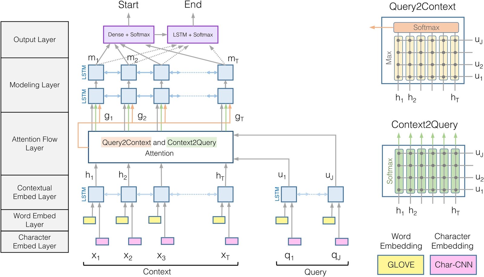
Figure 1: BiDirectional Attention Flow Model (best viewed in color)

图 1：双向注意力流模型（建议彩色查看）

Our machine comprehension model is a hierarchical multi-stage process and consists of six layers (Figure 1):

我们的机器阅读理解模型是一个层次化的多阶段过程，由六层组成（图 1）：

1. Character Embedding Layer maps each word to a vector space using character-level CNNs.

1. 字符嵌入层用字符级卷积网络，把每个词映射到一个向量空间。

2. Word Embedding Layer maps each word to a vector space using a pre-trained word embedding model.

2. 词嵌入层用预训练的词嵌入模型，把每个词映射到一个向量空间。

3. Contextual Embedding Layer utilizes contextual cues from surrounding words to refine the embedding of the words. These first three layers are applied to both the query and context.

3. 上下文嵌入层利用来自周围词的上下文线索，来精细调整词的嵌入。前三层同时应用于查询和上下文。

4. Attention Flow Layer couples the query and context vectors and produces a set of query-aware feature vectors for each word in the context.

4. 注意力流层把查询向量和上下文向量耦合起来，为上下文中的每个词产生一组查询感知的特征向量。

5. Modeling Layer employs a Recurrent Neural Network to scan the context.

5. 建模层用循环神经网络扫描上下文。

6. Output Layer provides an answer to the query.

6. 输出层给出对查询的回答。

1. Character Embedding Layer.

Character embedding layer is responsible for mapping each word to a high-dimensional vector space. Let $\{\bm{x}_{1},\dots\bm{x}_{T}\}$ and $\{\bm{q}_{1},\dots\bm{q}_{J}\}$ represent the words in the input context paragraph and query, respectively. Following Kim (2014), we obtain the character-level embedding of each word using Convolutional Neural Networks (CNN). Characters are embedded into vectors, which can be considered as 1D inputs to the CNN, and whose size is the input channel size of the CNN. The outputs of the CNN are max-pooled over the entire width to obtain a fixed-size vector for each word.

1. 字符嵌入层。

字符嵌入层负责把每个词映射到一个高维向量空间。设 $\{\bm{x}_{1},\dots\bm{x}_{T}\}$ 和 $\{\bm{q}_{1},\dots\bm{q}_{J}\}$ 分别表示输入上下文段落和查询中的词。我们遵循 Kim (2014)，用卷积神经网络（CNN）得到每个词的字符级嵌入。字符先被嵌入成向量，这些向量可看成 CNN 的一维输入，其尺寸就是 CNN 的输入通道数。CNN 的输出在整个宽度上做最大池化，从而为每个词得到一个固定长度的向量。

2. Word Embedding Layer.

Word embedding layer also maps each word to a high-dimensional vector space. We use pre-trained word vectors, GloVe (Pennington et al., 2014), to obtain the fixed word embedding of each word.

2. 词嵌入层。

词嵌入层同样把每个词映射到一个高维向量空间。我们使用预训练词向量 GloVe（Pennington et al., 2014），得到每个词的固定词嵌入。

The concatenation of the character and word embedding vectors is passed to a two-layer Highway Network (Srivastava et al., 2015). The outputs of the Highway Network are two sequences of $d$-dimensional vectors, or more conveniently, two matrices: ${\bf X}\in\mathbb{R}^{d\times T}$ for the context and ${\bf Q}\in\mathbb{R}^{d\times J}$ for the query.

字符嵌入向量与词嵌入向量拼接后，送入一个两层的高速公路网络（Highway Network）（Srivastava et al., 2015）。高速公路网络的输出是两个 $d$ 维向量序列，或者更方便地写成两个矩阵：上下文为 ${\bf X}\in\mathbb{R}^{d\times T}$，查询为 ${\bf Q}\in\mathbb{R}^{d\times J}$。

3. Contextual Embedding Layer.

We use a Long Short-Term Memory Network (LSTM) (Hochreiter & Schmidhuber, 1997) on top of the embeddings provided by the previous layers to model the temporal interactions between words. We place an LSTM in both directions, and concatenate the outputs of the two LSTMs. Hence we obtain ${\bf H}\in\mathbb{R}^{2d\times T}$ from the context word vectors ${\bf X}$, and ${\bf U}\in\mathbb{R}^{2d\times J}$ from query word vectors ${\bf Q}$. Note that each column vector of ${\bf H}$ and ${\bf U}$ is $2d$-dimensional because of the concatenation of the outputs of the forward and backward LSTMs, each with $d$-dimensional output.

3. 上下文嵌入层。

我们在前几层给出的嵌入之上，使用长短期记忆网络（LSTM）（Hochreiter & Schmidhuber, 1997）来建模词与词之间的时间交互。我们在两个方向上各放一个 LSTM，并把两个 LSTM 的输出拼接起来。于是，由上下文词向量 ${\bf X}$ 得到 ${\bf H}\in\mathbb{R}^{2d\times T}$，由查询词向量 ${\bf Q}$ 得到 ${\bf U}\in\mathbb{R}^{2d\times J}$。需要说明的是，由于前向和后向 LSTM 的输出（各自为 $d$ 维）被拼接，${\bf H}$ 和 ${\bf U}$ 的每个列向量都是 $2d$ 维的。

It is worth noting that the first three layers of the model are computing features from the query and context at different levels of granularity, akin to the multi-stage feature computation of convolutional neural networks in the computer vision field.

值得指出的是，模型的前三层是在不同粒度上从查询和上下文计算特征，这类似于计算机视觉中卷积神经网络的多阶段特征计算。

4. Attention Flow Layer.

Attention flow layer is responsible for linking and fusing information from the context and the query words. Unlike previously popular attention mechanisms (Weston et al., 2015; Hill et al., 2016; Sordoni et al., 2016; Shen et al., 2016), the attention flow layer is not used to summarize the query and context into single feature vectors. Instead, the attention vector at each time step, along with the embeddings from previous layers, are allowed to flow through to the subsequent modeling layer. This reduces the information loss caused by early summarization.

4. 注意力流层。

注意力流层负责把来自上下文词和查询词的信息关联并融合起来。与此前流行的注意力机制（Weston et al., 2015; Hill et al., 2016; Sordoni et al., 2016; Shen et al., 2016）不同，注意力流层并不用来把查询和上下文收成单个特征向量。相反，每个时间步的注意力向量连同此前各层的嵌入，都被允许流向后续的建模层。这减少了过早摘要造成的信息损失。

The inputs to the layer are contextual vector representations of the context ${\bf H}$ and the query ${\bf U}$. The outputs of the layer are the query-aware vector representations of the context words, ${\bf G}$, along with the contextual embeddings from the previous layer.

该层的输入是上下文的上下文向量表示 ${\bf H}$ 和查询的上下文向量表示 ${\bf U}$。该层的输出是上下文词的查询感知向量表示 ${\bf G}$，以及来自上一层的上下文嵌入。

In this layer, we compute attentions in two directions: from context to query as well as from query to context. Both of these attentions, which will be discussed below, are derived from a shared similarity matrix, ${\bf S}\in\mathbb{R}^{T\times J}$, between the contextual embeddings of the context (${\bf H}$) and the query (${\bf U}$), where ${\bf S}_{tj}$ indicates the similarity between $t$-th context word and $j$-th query word. The similarity matrix is computed by

在这一层，我们在两个方向上计算注意力：从上下文到查询，以及从查询到上下文。下面将讨论的这两种注意力，都来自上下文的上下文嵌入（${\bf H}$）与查询的上下文嵌入（${\bf U}$）之间的共享相似度矩阵 ${\bf S}\in\mathbb{R}^{T\times J}$，其中 ${\bf S}_{tj}$ 表示第 $t$ 个上下文词与第 $j$ 个查询词之间的相似度。相似度矩阵由下式计算

$${\bf S}_{tj}=\alpha({\bf H}_{:t},{\bf U}_{:j})\in\mathbb{R} \tag{1}$$

where $\alpha$ is a trainable scalar function that encodes the similarity between its two input vectors, ${\bf H}_{:t}$ is $t$-th column vector of ${\bf H}$, and ${\bf U}_{:j}$ is $j$-th column vector of ${\bf U}$, We choose $\alpha({\bf h},{\bf u})={\bf w}^{\top}_{({\bf S})}[{\bf h};{\bf u};{\bf h}\circ{\bf u}]$, where ${\bf w}_{({\bf S})}\in\mathbb{R}^{6d}$ is a trainable weight vector, $\circ$ is elementwise multiplication, $[;]$ is vector concatenation across row, and implicit multiplication is matrix multiplication. Now we use ${\bf S}$ to obtain the attentions and the attended vectors in both directions.

其中 $\alpha$ 是一个可训练的标量函数，用来编码其两个输入向量之间的相似度，${\bf H}_{:t}$ 是 ${\bf H}$ 的第 $t$ 个列向量，${\bf U}_{:j}$ 是 ${\bf U}$ 的第 $j$ 个列向量。我们取 $\alpha({\bf h},{\bf u})={\bf w}^{\top}_{({\bf S})}[{\bf h};{\bf u};{\bf h}\circ{\bf u}]$，其中 ${\bf w}_{({\bf S})}\in\mathbb{R}^{6d}$ 是可训练的权重向量，$\circ$ 表示逐元素乘法，$[;]$ 表示按行拼接向量，而隐含的乘法是矩阵乘法。接下来我们用 ${\bf S}$ 得到两个方向上的注意力和已注意向量。

Context-to-query Attention. Context-to-query (C2Q) attention signifies which query words are most relevant to each context word. Let ${\bf a}_{t}\in\mathbb{R}^{J}$ represent the attention weights on the query words by $t$-th context word, $\sum{\bf a}_{tj}=1$ for all $t$. The attention weight is computed by ${\bf a}_{t}=\mathrm{softmax}({\bf S}_{t:})\in\mathbb{R}^{J}$, and subsequently each attended query vector is $\tilde{{\bf U}}_{:t}=\sum_{j}{\bf a}_{tj}{\bf U}_{:j}$. Hence $\tilde{{\bf U}}$ is a $2d$-by-$T$ matrix containing the attended query vectors for the entire context.

上下文到查询注意力。 上下文到查询（C2Q）注意力表示：对每个上下文词而言，哪些查询词最为相关。设 ${\bf a}_{t}\in\mathbb{R}^{J}$ 表示第 $t$ 个上下文词在查询词上的注意力权重，对所有 $t$ 都有 $\sum{\bf a}_{tj}=1$。注意力权重由 ${\bf a}_{t}=\mathrm{softmax}({\bf S}_{t:})\in\mathbb{R}^{J}$ 计算，随后每个已注意的查询向量为 $\tilde{{\bf U}}_{:t}=\sum_{j}{\bf a}_{tj}{\bf U}_{:j}$。因此 $\tilde{{\bf U}}$ 是一个 $2d\times T$ 的矩阵，包含整个上下文所对应的已注意查询向量。

Query-to-context Attention. Query-to-context (Q2C) attention signifies which context words have the closest similarity to one of the query words and are hence critical for answering the query. We obtain the attention weights on the context words by ${\bf b}=\mathrm{softmax}(\max_{col}({\bf S}))\in\mathbb{R}^{T}$, where the maximum function ($\max_{col}$) is performed across the column. Then the attended context vector is $\tilde{\bf h}=\sum_{t}{\bf b}_{t}{\bf H}_{:t}\in\mathbb{R}^{2d}$. This vector indicates the weighted sum of the most important words in the context with respect to the query. $\tilde{\bf h}$ is tiled $T$ times across the column, thus giving $\tilde{\bf H}\in\mathbb{R}^{2d\times T}$.

查询到上下文注意力。 查询到上下文（Q2C）注意力表示：哪些上下文词与某个查询词最为相近，因而对回答查询至关重要。我们用 ${\bf b}=\mathrm{softmax}(\max_{col}({\bf S}))\in\mathbb{R}^{T}$ 得到上下文词上的注意力权重，其中最大值函数（$\max_{col}$）沿列进行。然后，已注意的上下文向量为 $\tilde{\bf h}=\sum_{t}{\bf b}_{t}{\bf H}_{:t}\in\mathbb{R}^{2d}$。这个向量表示相对查询而言上下文中最重要的那些词的加权和。再把 $\tilde{\bf h}$ 沿列复制 $T$ 次，得到 $\tilde{\bf H}\in\mathbb{R}^{2d\times T}$。

Finally, the contextual embeddings and the attention vectors are combined together to yield ${\bf G}$, where each column vector can be considered as the query-aware representation of each context word. We define ${\bf G}$ by

最后，把上下文嵌入和注意力向量组合起来得到 ${\bf G}$，其中每个列向量都可以看成每个上下文词的查询感知表示。我们把 ${\bf G}$ 定义为

$${\bf G}_{:t}={\bm{\beta}}({\bf H}_{:t},\tilde{\bf U}_{:t},\tilde{\bf H}_{:t})\in\mathbb{R}^{d_{\bf G}} \tag{2}$$

where ${\bf G}_{:t}$ is the $t$-th column vector (corresponding to $t$-th context word), ${\bm{\beta}}$ is a trainable vector function that fuses its (three) input vectors, and $d_{\bf G}$ is the output dimension of the ${\bm{\beta}}$ function. While the ${\bm{\beta}}$ function can be an arbitrary trainable neural network, such as multi-layer perceptron, a simple concatenation as following still shows good performance in our experiments: ${\bm{\beta}}({\bf h},\tilde{\bf u},\tilde{\bf h})=[{\bf h};\tilde{\bf u};{\bf h}\circ\tilde{\bf u};{\bf h}\circ\tilde{\bf h}]\in\mathbb{R}^{8d\times T}$ (i.e., $d_{\bf G}=8d$).

其中 ${\bf G}_{:t}$ 是第 $t$ 个列向量（对应于第 $t$ 个上下文词），${\bm{\beta}}$ 是一个可训练的向量函数，用来融合其（三个）输入向量，$d_{\bf G}$ 是 ${\bm{\beta}}$ 函数的输出维数。虽然 ${\bm{\beta}}$ 函数可以是任意可训练的神经网络，例如多层感知机，但在我们的实验中，如下这种简单的拼接仍然表现很好：${\bm{\beta}}({\bf h},\tilde{\bf u},\tilde{\bf h})=[{\bf h};\tilde{\bf u};{\bf h}\circ\tilde{\bf u};{\bf h}\circ\tilde{\bf h}]\in\mathbb{R}^{8d\times T}$（也就是 $d_{\bf G}=8d$）。

5. Modeling Layer.

The input to the modeling layer is ${\bf G}$, which encodes the query-aware representations of context words. The output of the modeling layer captures the interaction among the context words conditioned on the query. This is different from the contextual embedding layer, which captures the interaction among context words independent of the query. We use two layers of bi-directional LSTM, with the output size of $d$ for each direction. Hence we obtain a matrix ${\bf M}\in\mathbb{R}^{2d\times T}$, which is passed onto the output layer to predict the answer. Each column vector of ${\bf M}$ is expected to contain contextual information about the word with respect to the entire context paragraph and the query.

5. 建模层。

建模层的输入是 ${\bf G}$，它编码了上下文词的查询感知表示。建模层的输出刻画的是在以查询为条件时，上下文词之间的交互。这与上下文嵌入层不同，后者刻画的是与查询无关的上下文词之间的交互。我们使用两层双向 LSTM，每个方向的输出大小为 $d$。于是得到矩阵 ${\bf M}\in\mathbb{R}^{2d\times T}$，再把它送到输出层去预测答案。${\bf M}$ 的每个列向量，预期包含该词相对整段上下文以及查询的上下文信息。

6. Output Layer.

The output layer is application-specific. The modular nature of BiDAF allows us to easily swap out the output layer based on the task, with the rest of the architecture remaining exactly the same. Here, we describe the output layer for the QA task. In section 5, we use a slight modification of this output layer for cloze-style comprehension.

6. 输出层。

输出层是与具体应用相关的。BiDAF 的模块化设计使我们能够根据任务方便地替换输出层，而其余结构保持不变。这里我们描述面向问答任务的输出层。在第 5 节，我们会对这一输出层做少许修改，用于完形填空式的阅读理解。

The QA task requires the model to find a sub-phrase of the paragraph to answer the query. The phrase is derived by predicting the start and the end indices of the phrase in the paragraph. We obtain the probability distribution of the start index over the entire paragraph by

问答任务要求模型在段落中找到一个子短语来回答查询。这个短语通过预测它在段落中的起始和结束下标得到。我们用下式得到起始下标在整段上的概率分布

$${\bf p}^{1}=\mathrm{softmax}({\bf w}_{({\bf p}^{1})}^{\top}[{\bf G};{\bf M}]), \tag{3}$$

where ${\bf w}_{({\bf p}^{1})}\in\mathbb{R}^{10d}$ is a trainable weight vector. For the end index of the answer phrase, we pass ${\bf M}$ to another bidirectional LSTM layer and obtain ${\bf M}^{2}\in\mathbb{R}^{2d\times T}$. Then we use ${\bf M}^{2}$ to obtain the probability distribution of the end index in a similar manner:

其中 ${\bf w}_{({\bf p}^{1})}\in\mathbb{R}^{10d}$ 是可训练的权重向量。对于答案短语的结束下标，我们把 ${\bf M}$ 再送入一层双向 LSTM，得到 ${\bf M}^{2}\in\mathbb{R}^{2d\times T}$。然后用类似的方式，由 ${\bf M}^{2}$ 得到结束下标的概率分布：

$${\bf p}^{2}=\mathrm{softmax}({\bf w}_{({\bf p}^{2})}^{\top}[{\bf G};{\bf M}^{2}]) \tag{4}$$

Training. We define the training loss (to be minimized) as the sum of the negative log probabilities of the true start and end indices by the predicted distributions, averaged over all examples:

训练。 我们将要最小化的训练损失，定义为真实起始和结束下标在预测分布下的负对数概率之和，再对所有样本取平均：

$$L(\theta)=-\frac{1}{N}\sum^{N}_{i}\log({\bf p}^{1}_{y^{1}_{i}})+\log({\bf p}^{2}_{y^{2}_{i}}) \tag{5}$$

where $\theta$ is the set of all trainable weights in the model (the weights and biases of CNN filters and LSTM cells, ${\bf w}_{({\bf S})}$, ${\bf w}_{({\bf p}^{1})}$ and ${\bf w}_{({\bf p}^{2})}$), $N$ is the number of examples in the dataset, $y^{1}_{i}$ and $y^{2}_{i}$ are the true start and end indices of the $i$-th example, respectively, and ${\bf p}_{k}$ indicates the $k$-th value of the vector ${\bf p}$.

其中 $\theta$ 是模型中全部可训练权重的集合（CNN 滤波器和 LSTM 单元的权重与偏置，以及 ${\bf w}_{({\bf S})}$、${\bf w}_{({\bf p}^{1})}$ 和 ${\bf w}_{({\bf p}^{2})}$），$N$ 是数据集中的样本数，$y^{1}_{i}$ 和 $y^{2}_{i}$ 分别是第 $i$ 个样本的真实起始和结束下标，${\bf p}_{k}$ 表示向量 ${\bf p}$ 的第 $k$ 个值。

Test. The answer span $(k,l)$ where $k\leq l$ with the maximum value of ${\bf p}^{1}_{k}{\bf p}^{2}_{l}$ is chosen, which can be computed in linear time with dynamic programming.

测试。 选取满足 $k\leq l$ 且 ${\bf p}^{1}_{k}{\bf p}^{2}_{l}$ 最大的答案跨度 $(k,l)$，这可以用动态规划在线性时间内算出来。

3 Related Work

3 相关工作

Machine comprehension.

A significant contributor to the advancement of MC models has been the availability of large datasets. Early datasets such as MCTest (Richardson et al., 2013) were too small to train end-to-end neural models. Massive cloze test datasets (CNN/DailyMail by Hermann et al. (2015) and Childrens Book Test by Hill et al. (2016)), enabled the application of deep neural architectures to this task. More recently, Rajpurkar et al. (2016) released the Stanford Question Answering (SQuAD) dataset with over 100,000 questions. We evaluate the performance of our comprehension system on both SQuAD and CNN/DailyMail datasets.

机器阅读理解。

推动阅读理解模型进展的一个重要因素，是大型数据集的出现。早期数据集如 MCTest（Richardson et al., 2013）规模太小，无法训练端到端的神经模型。大规模完形填空数据集（Hermann et al. (2015) 的 CNN/DailyMail，以及 Hill et al. (2016) 的 Children’s Book Test）使得深度神经结构可以用于这一任务。更近一些，Rajpurkar et al. (2016) 发布了包含十万余个问题的斯坦福问答（SQuAD）数据集。我们在 SQuAD 和 CNN/DailyMail 两个数据集上评估阅读理解系统的表现。

Previous works in end-to-end machine comprehension use attention mechanisms in three distinct ways. The first group (largely inspired by Bahdanau et al. (2015)) uses a dynamic attention mechanism, in which the attention weights are updated dynamically given the query and the context as well as the previous attention. Hermann et al. (2015) argue that the dynamic attention model performs better than using a single fixed query vector to attend on context words on CNN & DailyMail datasets. Chen et al. (2016) show that simply using bilinear term for computing the attention weights in the same model drastically improves the accuracy. Wang & Jiang (2016) reverse the direction of the attention (attending on query words as the context RNN progresses) for SQuAD. In contrast to these models, BiDAF uses a memory-less attention mechanism.

此前的端到端机器阅读理解工作，以三种不同方式使用注意力机制。第一组（很大程度上受 Bahdanau et al. (2015) 启发）使用动态注意力机制，注意力权重会根据查询、上下文以及前一步注意力动态更新。Hermann et al. (2015) 认为，在 CNN 与 DailyMail 数据集上，动态注意力模型比用一个固定的查询向量去注意上下文词表现更好。Chen et al. (2016) 表明，在同一模型中只需用双线性项计算注意力权重，精度就会大幅提高。Wang & Jiang (2016) 把注意力的方向反过来（随着上下文 RNN 推进去注意查询词），用于 SQuAD。与这些模型不同，BiDAF 使用无记忆的注意力机制。

The second group computes the attention weights once, which are then fed into an output layer for final prediction (e.g., Kadlec et al. (2016)). Attention-over-attention model (Cui et al., 2016) uses a 2D similarity matrix between the query and context words (similar to Equation 1) to compute the weighted average of query-to-context attention. In contrast to these models, BiDAF does not summarize the two modalities in the attention layer and instead lets the attention vectors flow into the modeling (RNN) layer.

第二组只计算一次注意力权重，再把它送入输出层做最终预测（例如 Kadlec et al. (2016)）。Attention-over-attention 模型（Cui et al., 2016）使用查询词与上下文词之间的二维相似度矩阵（类似于式 1）来计算查询到上下文注意力的加权平均。与这些模型不同，BiDAF 并不在注意力层把两种模态做摘要，而是让注意力向量流入建模（RNN）层。

The third group (considered as variants of Memory Network (Weston et al., 2015)) repeats computing an attention vector between the query and the context through multiple layers, typically referred to as multi-hop (Sordoni et al., 2016; Dhingra et al., 2016). Shen et al. (2016) combine Memory Networks with Reinforcement Learning in order to dynamically control the number of hops. One can also extend our BiDAF model to incorporate multiple hops.

第三组（可看成记忆网络（Weston et al., 2015）的变体）通过多层重复计算查询与上下文之间的注意力向量，通常称为多跳（Sordoni et al., 2016; Dhingra et al., 2016）。Shen et al. (2016) 把记忆网络与强化学习结合起来，以便动态控制跳数。也可以把我们的 BiDAF 模型扩展到包含多次跳跃。

Visual question answering.

The task of question answering has also gained a lot of interest in the computer vision community. Early works on visual question answering (VQA) involved encoding the question using an RNN, encoding the image using a CNN and combining them to answer the question (Antol et al., 2015; Malinowski et al., 2015). Attention mechanisms have also been successfully employed for the VQA task and can be broadly clustered based on the granularity of their attention and the approach to construct the attention matrix. At the coarse level of granularity, the question attends to different patches in the image (Zhu et al., 2016; Xiong et al., 2016a). At a finer level, each question word attends to each image patch and the highest attention value for each spatial location (Xu & Saenko, 2016) is adopted. A hybrid approach is to combine questions representations at multiple levels of granularity (unigrams, bigrams, trigrams) (Yang et al., 2015). Several approaches to constructing the attention matrix have been used including element-wise product, element-wise sum, concatenation and Multimodal Compact Bilinear Pooling (Fukui et al., 2016).

视觉问答。

问答任务在计算机视觉社区同样引起了很大兴趣。早期的视觉问答（VQA）工作用 RNN 编码问题、用 CNN 编码图像，再把二者结合起来回答问题（Antol et al., 2015; Malinowski et al., 2015）。注意力机制也被成功地用于 VQA 任务，并可以大致按注意力的粒度以及构造注意力矩阵的方法来分组。在较粗的粒度上，问题去注意图像中的不同区块（Zhu et al., 2016; Xiong et al., 2016a）。在更细的粒度上，每个问题词去注意每个图像区块，并采用每个空间位置上的最高注意力值（Xu & Saenko, 2016）。一种混合做法是把多个粒度上的问题表示（unigram、bigram、trigram）结合起来（Yang et al., 2015）。构造注意力矩阵的方法也有多种，包括逐元素乘积、逐元素求和、拼接，以及多模态紧致双线性池化（Fukui et al., 2016）。

Lu et al. (2016) have recently shown that in addition to attending from the question to image patches, attending from the image back to the question words provides an improvement on the VQA task. This finding in the visual domain is consistent with our finding in the language domain, where our bi-directional attention between the query and context provides improved results. Their model, however, uses the attention weights directly in the output layer and does not take advantage of the attention flow to the modeling layer.

Lu et al. (2016) 最近表明，除了从问题去注意图像区块，再从图像回到问题词上做注意，也能提高 VQA 任务的成绩。这一来自视觉领域的发现，与我们在语言领域的发现一致：查询与上下文之间的双向注意力能带来更好的结果。不过，他们的模型直接把注意力权重用在输出层，并没有利用注意力流向建模层这一点。

4 Question Answering Experiments

4 问答实验

In this section, we evaluate our model on the task of question answering using the recently released SQuAD (Rajpurkar et al., 2016), which has gained a huge attention over a few months. In the next section, we evaluate our model on the task of cloze-style reading comprehension.

本节我们在最近发布的、短短几个月就受到广泛关注的 SQuAD（Rajpurkar et al., 2016）上，评估模型在问答任务上的表现。下一节再评估完形填空式阅读理解。

Dataset.

SQuAD is a machine comprehension dataset on a large set of Wikipedia articles, with more than 100,000 questions. The answer to each question is always a span in the context. The model is given a credit if its answer matches one of the human written answers. Two metrics are used to evaluate models: Exact Match (EM) and a softer metric, F1 score, which measures the weighted average of the precision and recall rate at character level. The dataset consists of 90k/10k train/dev question-context tuples with a large hidden test set. It is one of the largest available MC datasets with human-written questions and serves as a great test bed for our model.

数据集。

SQuAD 是建立在大量维基百科文章上的机器阅读理解数据集，问题超过十万个。每个问题的答案都是上下文中的一个跨度。若模型的答案与某一条人工书写的答案匹配，就算答对。评估使用两个指标：精确匹配（EM），以及更宽松的、在字符级衡量精确率和召回率加权平均的 F1 分数。数据集包含 9 万/1 万的训练/开发问题–上下文对，以及一个较大的隐藏测试集。它是当时规模最大的、带有人工书写问题的阅读理解数据集之一，很适合用来检验我们的模型。

Model Details.

The model architecture used for this task is depicted in Figure 1. Each paragraph and question are tokenized by a regular-expression-based word tokenizer (PTB Tokenizer) and fed into the model. We use 100 1D filters for CNN char embedding, each with a width of 5. The hidden state size ($d$) of the model is 100. The model has about 2.6 million parameters. We use the AdaDelta (Zeiler, 2012) optimizer, with a minibatch size of 60 and an initial learning rate of $0.5$, for 12 epochs. A dropout (Srivastava et al., 2014) rate of $0.2$ is used for the CNN, all LSTM layers, and the linear transformation before the softmax for the answers. During training, the moving averages of all weights of the model are maintained with the exponential decay rate of $0.999$. At test time, the moving averages instead of the raw weights are used. The training process takes roughly 20 hours on a single Titan X GPU. We also train an ensemble model consisting of 12 training runs with the identical architecture and hyper-parameters. At test time, we choose the answer with the highest sum of confidence scores amongst the 12 runs for each question.

模型细节。

该任务所用的模型结构如图 1 所示。每段文字和每个问题都用基于正则表达式的分词器（PTB Tokenizer）分词后送入模型。字符嵌入 CNN 使用 100 个一维滤波器，每个宽度为 5。模型的隐状态大小（$d$）为 100。模型约有 260 万个参数。我们使用 AdaDelta（Zeiler, 2012）优化器，小批量大小为 60，初始学习率为 $0.5$，训练 12 个周期。CNN、全部 LSTM 层，以及答案 softmax 之前的线性变换，都使用 $0.2$ 的 dropout（Srivastava et al., 2014）。训练过程中，模型全部权重的滑动平均以 $0.999$ 的指数衰减率维护。测试时使用滑动平均，而不是原始权重。整个训练过程在一块 Titan X GPU 上大约需要 20 小时。我们还训练了一个由 12 次结构与超参数完全相同的训练构成的集成模型。测试时，对每个问题选取 12 次运行中置信度分数之和最高的答案。

Results.

The results of our model and competing approaches on the hidden test are summarized in Table 1a. BiDAF (ensemble) achieves an EM score of 73.3 and an F1 score of 81.1, outperforming all previous approaches.

结果。

我们的模型与竞品方法在隐藏测试集上的结果汇总于表 1a。BiDAF（集成）取得了 73.3 的 EM 和 81.1 的 F1，超过了此前所有方法。

	Single Model	Ensemble
	EM	F1	EM	F1
Logistic Regression Baselinea	40.4	51.0	-	-
Dynamic Chunk Readerb	62.5	71.0	-	-
Fine-Grained Gatingc	62.5	73.3	-	-
Match-LSTMd	64.7	73.7	67.9	77.0
Multi-Perspective Matchinge	65.5	75.1	68.2	77.2
Dynamic Coattention Networksf	66.2	75.9	71.6	80.4
R-Netg	68.4	77.5	72.1	79.7
BiDAF (Ours)	68.0	77.3	73.3	81.1

	EM	F1
No char embedding	65.0	75.4
No word embedding	55.5	66.8
No C2Q attention	57.2	67.7
No Q2C attention	63.6	73.7
Dynamic attention	63.5	73.6
BiDAF (single)	67.7	77.3
BiDAF (ensemble)	72.6	80.7

(a) Results on the SQuAD test set

(b) Ablations on the SQuAD dev set

Table 1: (1a) The performance of our model BiDAF and competing approaches by Rajpurkar et al. (2016)a, Yu et al. (2016)b, Yang et al. (2016)c, Wang & Jiang (2016)d, IBM Watson e (unpublished), Xiong et al. (2016b)f, and Microsoft Research Asia g (unpublished) on the SQuAD test set. A concurrent work by Lee et al. (2016) does not report the test scores. All results shown here reflect the SQuAD leaderboard (stanford-qa.com) as of 6 Dec 2016, 12pm PST. (1b) The performance of our model and its ablations on the SQuAD dev set. Ablation results are presented only for single runs.

	单模型	集成
	EM	F1	EM	F1
Logistic Regression Baselinea	40.4	51.0	-	-
Dynamic Chunk Readerb	62.5	71.0	-	-
Fine-Grained Gatingc	62.5	73.3	-	-
Match-LSTMd	64.7	73.7	67.9	77.0
Multi-Perspective Matchinge	65.5	75.1	68.2	77.2
Dynamic Coattention Networksf	66.2	75.9	71.6	80.4
R-Netg	68.4	77.5	72.1	79.7
BiDAF（本文）	68.0	77.3	73.3	81.1

	EM	F1
无字符嵌入	65.0	75.4
无词嵌入	55.5	66.8
无 C2Q 注意力	57.2	67.7
无 Q2C 注意力	63.6	73.7
动态注意力	63.5	73.6
BiDAF（单模型）	67.7	77.3
BiDAF（集成）	72.6	80.7

(a) 在 SQuAD 测试集上的结果

(b) 在 SQuAD 开发集上的消融

表 1：(1a) 我们的模型 BiDAF 与竞品方法在 SQuAD 测试集上的表现，竞品包括 Rajpurkar et al. (2016)a、Yu et al. (2016)b、Yang et al. (2016)c、Wang & Jiang (2016)d、IBM Watson e（未发表）、Xiong et al. (2016b)f，以及微软亚洲研究院 g（未发表）。Lee et al. (2016) 的同期工作没有报告测试分数。这里列出的全部结果，反映的是截至 2016 年 12 月 6 日中午 12 点（太平洋标准时间）的 SQuAD 排行榜（stanford-qa.com）。(1b) 我们的模型及其消融在 SQuAD 开发集上的表现。消融结果只报告单次运行。

Ablations.

Table 1b shows the performance of our model and its ablations on the SQuAD dev set. Both char-level and word-level embeddings contribute towards the model’s performance. We conjecture that word-level embedding is better at representing the semantics of each word as a whole, while char-level embedding can better handle out-of-vocab (OOV) or rare words. To evaluate bi-directional attention, we remove C2Q and Q2C attentions. For ablating C2Q attention, we replace the attended question vector $\tilde{\bf U}$ with the average of the output vectors of the question’s contextual embedding layer (LSTM). C2Q attention proves to be critical with a drop of more than 10 points on both metrics. For ablating Q2C attention, the output of the attention layer, ${\bf G}$, does not include terms that have the attended Q2C vectors, $\tilde{\bf H}$. To evaluate the attention flow, we study a dynamic attention model, where the attention is dynamically computed within the modeling layer’s LSTM, following previous work (Bahdanau et al., 2015; Wang & Jiang, 2016). This is in contrast with our approach, where the attention is pre-computed before flowing to the modeling layer. Despite being a simpler attention mechanism, our proposed static attention outperforms the dynamically computed attention by more than 3 points. We conjecture that separating out the attention layer results in a richer set of features computed in the first 4 layers which are then incorporated by the modeling layer. We also show the performance of BiDAF with several different definitions of $\alpha$ and ${\bm{\beta}}$ functions (Equation 1 and 2) in Appendix B.

消融。

表 1b 给出了我们的模型及其消融在 SQuAD 开发集上的表现。字符级和词级嵌入都对模型表现有贡献。我们猜想，词级嵌入更善于表示每个词作为整体的语义，而字符级嵌入更能处理未登录词（OOV）或罕见词。为了评估双向注意力，我们去掉 C2Q 和 Q2C 注意力。去掉 C2Q 注意力时，我们把已注意的问题向量 $\tilde{\bf U}$ 替换成问题上下文嵌入层（LSTM）输出向量的平均。C2Q 注意力被证明至关重要，两个指标都会下降十个点以上。去掉 Q2C 注意力时，注意力层的输出 ${\bf G}$ 不再包含带有已注意 Q2C 向量 $\tilde{\bf H}$ 的那些项。为了评估注意力流，我们研究了一种动态注意力模型：注意力在建模层的 LSTM 内部动态计算，做法遵循此前工作（Bahdanau et al., 2015; Wang & Jiang, 2016）。这与我们的方法形成对照，我们是把注意力预先算好再流入建模层。尽管所提出的静态注意力机制更简单，它仍比动态计算的注意力高出三个点以上。我们猜想，把注意力层单独分出来，会使前四层算出更丰富的特征，再由建模层加以整合。我们还在附录 B 中给出了 BiDAF 在若干不同的 $\alpha$ 和 ${\bm{\beta}}$ 函数定义（式 1 和式 2）下的表现。

Visualizations.

We now provide a qualitative analysis of our model on the SQuAD dev set. First, we visualize the feature spaces after the word and contextual embedding layers. These two layers are responsible for aligning the embeddings between the query and context words which are the inputs to the subsequent attention layer. To visualize the embeddings, we choose a few frequent query words in the dev data and look at the context words that have the highest cosine similarity to the query words (Table 2). At the word embedding layer, query words such as When, Where and Who are not well aligned to possible answers in the context, but this dramatically changes in the contextual embedding layer which has access to context from surrounding words and is just 1 layer below the attention layer. When begins to match years, Where matches locations, and Who matches names.

可视化。

我们接下来在 SQuAD 开发集上对模型做定性分析。首先，我们可视化词嵌入层和上下文嵌入层之后的特征空间。这两层负责对齐查询词与上下文词的嵌入，它们是后续注意力层的输入。为了可视化这些嵌入，我们在开发数据中选取若干频繁出现的查询词，并观察与这些查询词余弦相似度最高的上下文词（表 2）。在词嵌入层，像 When、Where 和 Who 这样的查询词，与上下文中可能的答案对齐得并不好；但到了能够利用周围词上下文、并且就在注意力层之下一层的上下文嵌入层，情况发生了明显变化：When 开始匹配年份，Where 匹配地点，Who 匹配人名。

Layer	Query	Closest words in the Context using cosine similarity
Word	When	when, When, After, after, He, he, But, but, before, Before
Contextual	When	When, when, 1945, 1991, 1971, 1967, 1990, 1972, 1965, 1953
Word	Where	Where, where, It, IT, it, they, They, that, That, city
Contextual	Where	where, Where, Rotterdam, area, Nearby, location, outside, Area, across, locations
Word	Who	Who, who, He, he, had, have, she, She, They, they
Contextual	Who	who, whose, whom, Guiscard, person, John, Thomas, families, Elway, Louis
Word	city	City, city, town, Town, Capital, capital, district, cities, province, Downtown
Contextual	city	city, City, Angeles, Paris, Prague, Chicago, Port, Pittsburgh, London, Manhattan
Word	January	July, December, June, October, January, September, February, April, November, March
Contextual	January	January, March, December, August, December, July, July, July, March, December
Word	Seahawks	Seahawks, Broncos, 49ers, Ravens, Chargers, Steelers, quarterback, Vikings, Colts, NFL
Contextual	Seahawks	Seahawks, Broncos, Panthers, Vikings, Packers, Ravens, Patriots, Falcons, Steelers, Chargers
Word	date	date, dates, until, Until, June, July, Year, year, December, deadline
Contextual	date	date, dates, December, July, January, October, June, November, March, February

Table 2: Closest context words to a given query word, using a cosine similarity metric computed in the Word Embedding feature space and the Phrase Embedding feature space.

层	查询	用余弦相似度得到的、上下文中最近的词
词	When	when, When, After, after, He, he, But, but, before, Before
上下文	When	When, when, 1945, 1991, 1971, 1967, 1990, 1972, 1965, 1953
词	Where	Where, where, It, IT, it, they, They, that, That, city
上下文	Where	where, Where, Rotterdam, area, Nearby, location, outside, Area, across, locations
词	Who	Who, who, He, he, had, have, she, She, They, they
上下文	Who	who, whose, whom, Guiscard, person, John, Thomas, families, Elway, Louis
词	city	City, city, town, Town, Capital, capital, district, cities, province, Downtown
上下文	city	city, City, Angeles, Paris, Prague, Chicago, Port, Pittsburgh, London, Manhattan
词	January	July, December, June, October, January, September, February, April, November, March
上下文	January	January, March, December, August, December, July, July, July, March, December
词	Seahawks	Seahawks, Broncos, 49ers, Ravens, Chargers, Steelers, quarterback, Vikings, Colts, NFL
上下文	Seahawks	Seahawks, Broncos, Panthers, Vikings, Packers, Ravens, Patriots, Falcons, Steelers, Chargers
词	date	date, dates, until, Until, June, July, Year, year, December, deadline
上下文	date	date, dates, December, July, January, October, June, November, March, February

表 2：对给定查询词，在词嵌入特征空间和短语嵌入特征空间中，用余弦相似度度量得到的最接近的上下文词。

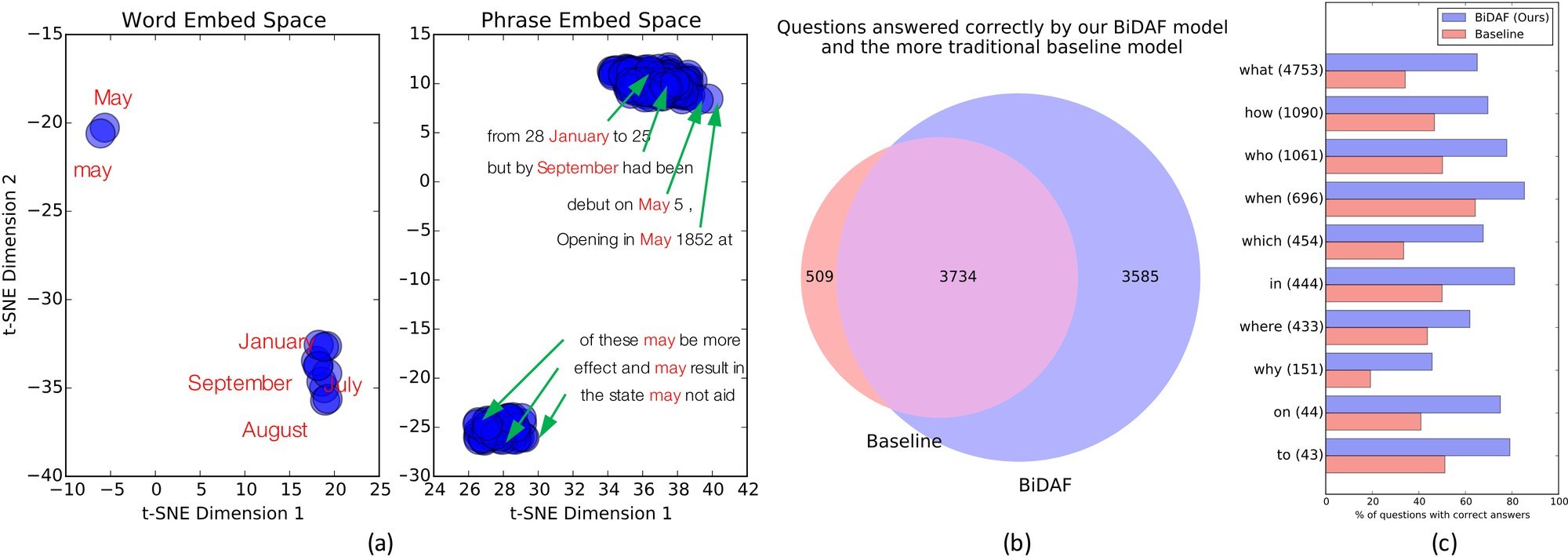
Figure 2: (a) t-SNE visualizations of the months names embedded in the two feature spaces. The contextual embedding layer is able to distinguish the two usages of the word May using context from the surrounding text. (b) Venn diagram of the questions answered correctly by our model and the more traditional baseline (Rajpurkar et al., 2016). (c) Correctly answered questions broken down by the 10 most frequent first words in the question.

图 2：(a) 两个特征空间中月份名称嵌入的 t-SNE 可视化。上下文嵌入层能够利用周围文本的上下文，区分 May 一词的两种用法。(b) 我们的模型与更传统的基线（Rajpurkar et al., 2016）都答对的问题的维恩图。(c) 按问题中最常见的 10 个首词，对答对的问题做分解。

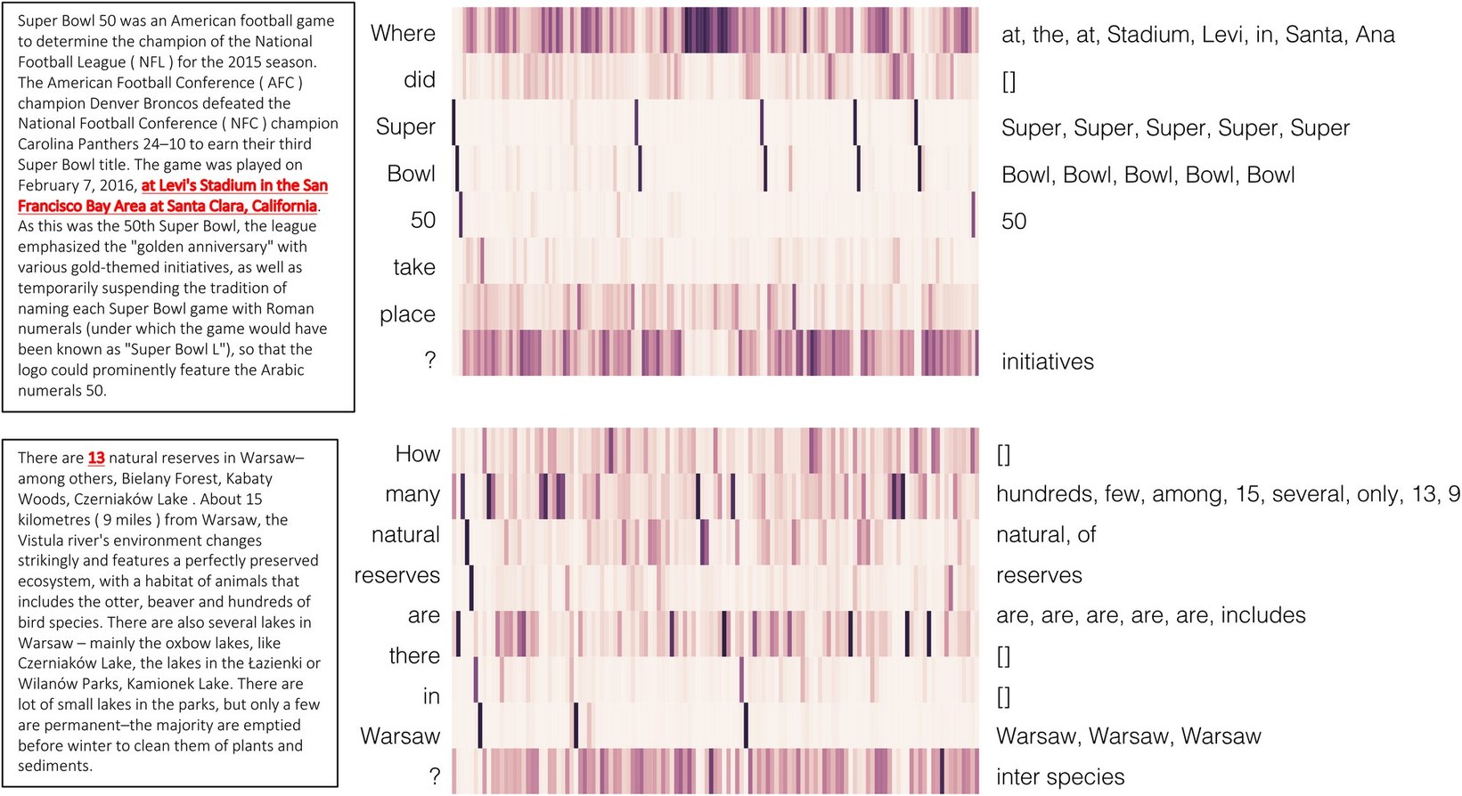
Figure 3: Attention matrices for question-context tuples. The left palette shows the context paragraph (correct answer in red and underlined), the middle palette shows the attention matrix (each row is a question word, each column is a context word), and the right palette shows the top attention points for each question word, above a threshold.

图 3：问题–上下文对上的注意力矩阵。左侧面板给出上下文段落（正确答案用红色并加下划线），中间面板给出注意力矩阵（每一行是一个问题词，每一列是一个上下文词），右侧面板给出每个问题词在某一阈值之上的主要注意位置。

We also visualize these two feature spaces using t-SNE in Figure 2. t-SNE is performed on a large fraction of dev data but we only plot data points corresponding to the months of the year. An interesting pattern emerges in the Word space, where May is separated from the rest of the months because May has multiple meanings in the English language. The contextual embedding layer uses contextual cues from surrounding words and is able to separate the usages of the word May. Finally we visualize the attention matrices for some question-context tuples in the dev data in Figure 3. In the first example, Where matches locations and in the second example, many matches quantities and numerical symbols. Also, entities in the question typically attend to the same entities in the context, thus providing a feature for the model to localize possible answers.

我们还在图 2 中用 t-SNE 可视化这两个特征空间。t-SNE 是在很大一部分开发数据上计算的，但我们只画出对应于各个月份的数据点。词空间中出现了一个有趣的模式：May 与其余月份分开了，因为 May 在英语中有多种含义。上下文嵌入层利用来自周围词的上下文线索，能够把 May 一词的不同用法分开。最后，我们在图 3 中可视化开发数据里一些问题–上下文对上的注意力矩阵。在第一个例子中，Where 匹配地点；在第二个例子中，many 匹配数量和数字符号。此外，问题中的实体通常会注意到上下文中的同一实体，从而为模型定位可能的答案提供特征。

Discussions.

We analyse the performance of our our model with a traditional language-feature-based baseline (Rajpurkar et al., 2016). Figure 2b shows a Venn diagram of the dev set questions correctly answered by the models. Our model is able to answer more than 86% of the questions correctly answered by the baseline. The 14% that are incorrectly answered does not have a clear pattern. This suggests that neural architectures are able to exploit much of the information captured by the language features. We also break this comparison down by the first words in the questions (Figure 2c). Our model outperforms the traditional baseline comfortably in every category.

讨论。

我们把模型的表现与一种基于传统语言特征的基线（Rajpurkar et al., 2016）做了分析。图 2b 给出了开发集上被各模型答对的问题的维恩图。基线答对的问题中，我们的模型也能答对其中 86% 以上。那 14% 答错的问题没有清晰的模式。这说明神经结构能够利用语言特征所捕捉到的大部分信息。我们还按问题的首词把这一比较拆开（图 2c）。在每一个类别上，我们的模型都明显超过传统基线。

Error Analysis.

We randomly select 50 incorrect questions (based on EM) and categorize them into 6 classes. 50% of errors are due to the imprecise boundaries of the answers, 28% involve syntactic complications and ambiguities, 14% are paraphrase problems, 4% require external knowledge, 2% need multiple sentences to answer, and 2% are due to mistakes during tokenization. See Appendix A for the examples of the error modes.

错误分析。

我们随机选取 50 个答错的问题（按 EM），并把它们分成 6 类。50% 的错误来自答案边界不够精确，28% 涉及句法上的复杂性和歧义，14% 是释义问题，4% 需要外部知识，2% 需要多句话才能回答，2% 则源于分词错误。各类错误模式的例子见附录 A。

5 Cloze Test Experiments

5 完形填空实验

We also evaluate our model on the task of cloze-style reading comprehension using the CNN and Daily Mail datasets (Hermann et al., 2015).

我们还在 CNN 和 Daily Mail 数据集（Hermann et al., 2015）上，评估模型在完形填空式阅读理解任务上的表现。

Dataset.

In a cloze test, the reader is asked to fill in words that have been removed from a passage, for measuring one’s ability to comprehend text. Hermann et al. (2015) have recently compiled a massive Cloze-style comprehension dataset, consisting of 300k/4k/3k and 879k/65k/53k (train/dev/test) examples from CNN and DailyMail news articles, respectively. Each example has a news article and an incomplete sentence extracted from the human-written summary of the article. To distinguish this task from language modeling and force one to refer to the article to predict the correct missing word, the missing word is always a named entity, anonymized with a random ID. Also, the IDs must be shuffled constantly during test, which is also critical for full anonymization.

数据集。

在完形填空测试中，读者被要求填上从段落中删去的词，以此来衡量理解文本的能力。Hermann et al. (2015) 最近汇编了一套大规模的完形填空式阅读理解数据集，分别来自 CNN 和 DailyMail 新闻文章，规模为 30 万/4 千/3 千以及 87.9 万/6.5 万/5.3 万（训练/开发/测试）。每个样本包含一篇新闻文章，以及从该文人工摘要中抽出的一个不完整句子。为了把这一任务与语言建模区分开，并迫使模型必须回到文章中才能预测被删掉的那个正确词，被删的词总是命名实体，并用一个随机 ID 匿名化。此外，测试时这些 ID 必须不断打乱，这对完全匿名化也很关键。

Model Details.

The model architecture used for this task is very similar to that for SQuAD (Section 4) with only a few small changes to adapt it to the cloze test. Since each answer in the CNN/DailyMail datasets is always a single word (entity), we only need to predict the start index (${\bf p}^{1}$); the prediction for the end index (${\bf p}^{2}$) is omitted from the loss function. Also, we mask out all non-entity words in the final classification layer so that they are forced to be excluded from possible answers. Another important difference from SQuAD is that the answer entity might appear more than once in the context paragraph. To address this, we follow a similar strategy from Kadlec et al. (2016). During training, after we obtain ${\bf p}^{1}$, we sum all probability values of the entity instances in the context that correspond to the correct answer. Then the loss function is computed from the summed probability. We use a minibatch size of 48 and train for 8 epochs, with early stop when the accuracy on validation data starts to drop. Inspired by the window-based method (Hill et al., 2016), we split each article into short sentences where each sentence is a 19-word window around each entity (hence the same word might appear in multiple sentences). The RNNs in BiDAF are not feed-forwarded or back-propagated across sentences, which speed up the training process by parallelization. The entire training process takes roughly 60 hours on eight Titan X GPUs. The other hyper-parameters are identical to the model described in Section 4.

模型细节。

该任务所用的模型结构与 SQuAD（第 4 节）非常相似，只做了少许改动以适应完形填空。由于 CNN/DailyMail 数据集中的每个答案都是单个词（实体），我们只需要预测起始下标（${\bf p}^{1}$）；结束下标（${\bf p}^{2}$）的预测从损失函数中去掉。此外，我们在最后的分类层把所有非实体词掩蔽掉，迫使它们不能成为候选答案。与 SQuAD 的另一个重要不同是，答案实体可能在上下文段落中出现不止一次。为此，我们采用与 Kadlec et al. (2016) 类似的策略。训练时，在得到 ${\bf p}^{1}$ 之后，我们把上下文中对应于正确答案的所有实体实例的概率值加总，再由这个加总后的概率计算损失函数。我们使用大小为 48 的小批量，训练 8 个周期，并在验证集准确率开始下降时提前停止。受基于窗口的方法（Hill et al., 2016）启发，我们把每篇文章切成短句，每个句子是环绕每个实体的 19 词窗口（因此同一个词可能出现在多个句子中）。BiDAF 中的 RNN 不在句子之间做前向传播或反向传播，从而可以通过并行化加快训练。整个训练过程在八块 Titan X GPU 上大约需要 60 小时。其余超参数与第 4 节描述的模型相同。

Results.

The results of our single-run models and competing approaches on the CNN/DailyMail datasets are summarized in Table 3. ∗ indicates ensemble methods. BiDAF outperforms previous single-run models on both datasets for both val and test data. On the DailyMail test, our single-run model even outperforms the best ensemble method.

结果。

我们的单次运行模型与竞品方法在 CNN/DailyMail 数据集上的结果汇总于表 3。∗ 表示集成方法。BiDAF 在两个数据集的验证集和测试集上，都超过了此前的单次运行模型。在 DailyMail 测试集上，我们的单次运行模型甚至超过了最好的集成方法。

	CNN	DailyMail
	val	test	val	test
Attentive Reader (Hermann et al., 2015)	61.6	63.0	70.5	69.0
MemNN (Hill et al., 2016)	63.4	6.8	-	-
AS Reader (Kadlec et al., 2016)	68.6	69.5	75.0	73.9
DER Network (Kobayashi et al., 2016)	71.3	72.9	-	-
Iterative Attention (Sordoni et al., 2016)	72.6	73.3	-	-
EpiReader (Trischler et al., 2016)	73.4	74.0	-	-
Stanford AR (Chen et al., 2016)	73.8	73.6	77.6	76.6
GAReader (Dhingra et al., 2016)	73.0	73.8	76.7	75.7
AoA Reader (Cui et al., 2016)	73.1	74.4	-	-
ReasoNet (Shen et al., 2016)	72.9	74.7	77.6	76.6
BiDAF (Ours)	76.3	76.9	80.3	79.6
MemNN∗ (Hill et al., 2016)	66.2	69.4	-	-
ASReader∗ (Kadlec et al., 2016)	73.9	75.4	78.7	77.7
Iterative Attention∗ (Sordoni et al., 2016)	74.5	75.7	-	-
GA Reader∗ (Dhingra et al., 2016)	76.4	77.4	79.1	78.1
Stanford AR∗ (Chen et al., 2016)	77.2	77.6	80.2	79.2

Table 3: Results on CNN/DailyMail datasets. We also include the results of previous ensemble methods (marked with ∗) for completeness.

	CNN	DailyMail
	验证	测试	验证	测试
Attentive Reader（Hermann et al., 2015）	61.6	63.0	70.5	69.0
MemNN（Hill et al., 2016）	63.4	6.8	-	-
AS Reader（Kadlec et al., 2016）	68.6	69.5	75.0	73.9
DER Network（Kobayashi et al., 2016）	71.3	72.9	-	-
Iterative Attention（Sordoni et al., 2016）	72.6	73.3	-	-
EpiReader（Trischler et al., 2016）	73.4	74.0	-	-
Stanford AR（Chen et al., 2016）	73.8	73.6	77.6	76.6
GAReader（Dhingra et al., 2016）	73.0	73.8	76.7	75.7
AoA Reader（Cui et al., 2016）	73.1	74.4	-	-
ReasoNet（Shen et al., 2016）	72.9	74.7	77.6	76.6
BiDAF（本文）	76.3	76.9	80.3	79.6
MemNN∗（Hill et al., 2016）	66.2	69.4	-	-
ASReader∗（Kadlec et al., 2016）	73.9	75.4	78.7	77.7
Iterative Attention∗（Sordoni et al., 2016）	74.5	75.7	-	-
GA Reader∗（Dhingra et al., 2016）	76.4	77.4	79.1	78.1
Stanford AR∗（Chen et al., 2016）	77.2	77.6	80.2	79.2

表 3：在 CNN/DailyMail 数据集上的结果。为完整起见，我们也列入了此前集成方法（以 ∗ 标记）的结果。

6 Conclusion

6 结论

In this paper, we introduce BiDAF, a multi-stage hierarchical process that represents the context at different levels of granularity and uses a bi-directional attention flow mechanism to achieve a query-aware context representation without early summarization. The experimental evaluations show that our model achieves the state-of-the-art results in Stanford Question Answering Dataset (SQuAD) and CNN/DailyMail cloze test. The ablation analyses demonstrate the importance of each component in our model. The visualizations and discussions show that our model is learning a suitable representation for MC and is capable of answering complex questions by attending to correct locations in the given paragraph. Future work involves extending our approach to incorporate multiple hops of the attention layer.

本文引入 BiDAF，这是一个分多阶段的层次化过程，在不同粒度上表示上下文，并用双向注意力流机制得到查询感知的上下文表示，而不做过早摘要。实验表明，我们的模型在斯坦福问答数据集（SQuAD）以及 CNN/DailyMail 完形填空测试上取得了当时最好的结果。消融分析说明了模型中每个组件的重要性。可视化和讨论表明，模型学到了适合于阅读理解的表示，并且能够通过注意到给定段落中的正确位置来回答复杂问题。未来工作包括把我们的方法扩展到包含注意力层的多次跳跃。

Acknowledgments

致谢

This research was supported by the NSF (IIS 1616112), NSF (III 1703166), Allen Institute for AI (66-9175), Allen Distinguished Investigator Award, Google Research Faculty Award, and Samsung GRO Award. We thank the anonymous reviewers for their helpful comments.

本研究得到 NSF（IIS 1616112）、NSF（III 1703166）、艾伦人工智能研究所（66-9175）、Allen Distinguished Investigator Award、Google Research Faculty Award 以及 Samsung GRO Award 的资助。我们感谢匿名审稿人的有益意见。

Footnotes

脚注

1. Our code and interactive demo are available at: allenai.github.io/bi-att-flow/

1. 我们的代码与交互演示见：allenai.github.io/bi-att-flow/

References

参考文献

Antol et al. (2015) Stanislaw Antol, Aishwarya Agrawal, Jiasen Lu, Margaret Mitchell, Dhruv Batra, C Lawrence Zitnick, and Devi Parikh. Vqa: Visual question answering. In ICCV , 2015.

Bahdanau et al. (2015) Dzmitry Bahdanau, Kyunghyun Cho, and Yoshua Bengio. Neural machine translation by jointly learning to align and translate. ICLR , 2015.

Chen et al. (2016) Danqi Chen, Jason Bolton, and Christopher D. Manning. A thorough examination of the cnn/daily mail reading comprehension task. In ACL , 2016.

Cui et al. (2016) Yiming Cui, Zhipeng Chen, Si Wei, Shijin Wang, Ting Liu, and Guoping Hu. Attention-over-attention neural networks for reading comprehension. arXiv preprint arXiv:1607.04423 , 2016.

Dhingra et al. (2016) Bhuwan Dhingra, Hanxiao Liu, William W Cohen, and Ruslan Salakhutdinov. Gated-attention readers for text comprehension. arXiv preprint arXiv:1606.01549 , 2016.

Fukui et al. (2016) Akira Fukui, Dong Huk Park, Daylen Yang, Anna Rohrbach, Trevor Darrell, and Marcus Rohrbach. Multimodal compact bilinear pooling for visual question answering and visual grounding. In EMNLP , 2016.

Hermann et al. (2015) Karl Moritz Hermann, Tomás Kociský, Edward Grefenstette, Lasse Espeholt, Will Kay, Mustafa Suleyman, and Phil Blunsom. Teaching machines to read and comprehend. In NIPS , 2015.

Hill et al. (2016) Felix Hill, Antoine Bordes, Sumit Chopra, and Jason Weston. The goldilocks principle: Reading children’s books with explicit memory representations. In ICLR , 2016.

Hochreiter & Schmidhuber (1997) Sepp Hochreiter and Jurgen Schmidhuber. Long short-term memory. Neural Computation , 1997.

Kadlec et al. (2016) Rudolf Kadlec, Martin Schmid, Ondrej Bajgar, and Jan Kleindienst. Text understanding with the attention sum reader network. In ACL , 2016.

Kim (2014) Yoon Kim. Convolutional neural networks for sentence classification. In EMNLP , 2014.

Kobayashi et al. (2016) Sosuke Kobayashi, Ran Tian, Naoaki Okazaki, and Kentaro Inui. Dynamic entity representation with max-pooling improves machine reading. In NAACL-HLT , 2016.

Lee et al. (2016) Kenton Lee, Tom Kwiatkowski, Ankur Parikh, and Dipanjan Das. Learning recurrent span representations for extractive question answering. arXiv preprint arXiv:1611.01436 , 2016.

Lu et al. (2016) Jiasen Lu, Jianwei Yang, Dhruv Batra, and Devi Parikh. Hierarchical question-image co-attention for visual question answering. In NIPS , 2016.

Malinowski et al. (2015) Mateusz Malinowski, Marcus Rohrbach, and Mario Fritz. Ask your neurons: A neural-based approach to answering questions about images. In ICCV , 2015.

Pennington et al. (2014) Jeffrey Pennington, Richard Socher, and Christopher D Manning. Glove: Global vectors for word representation. In EMNLP , 2014.

Rajpurkar et al. (2016) Pranav Rajpurkar, Jian Zhang, Konstantin Lopyrev, and Percy Liang. Squad: 100,000+ questions for machine comprehension of text. In EMNLP , 2016.

Richardson et al. (2013) Matthew Richardson, Christopher JC Burges, and Erin Renshaw. Mctest: A challenge dataset for the open-domain machine comprehension of text. In EMNLP , 2013.

Shen et al. (2016) Yelong Shen, Po-Sen Huang, Jianfeng Gao, and Weizhu Chen. Reasonet: Learning to stop reading in machine comprehension. arXiv preprint arXiv:1609.05284 , 2016.

Sordoni et al. (2016) Alessandro Sordoni, Phillip Bachman, and Yoshua Bengio. Iterative alternating neural attention for machine reading. arXiv preprint arXiv:1606.02245 , 2016.

Srivastava et al. (2014) Nitish Srivastava, Geoffrey E. Hinton, Alex Krizhevsky, Ilya Sutskever, and Ruslan Salakhutdinov. Dropout: a simple way to prevent neural networks from overfitting. JMLR , 2014.

Srivastava et al. (2015) Rupesh Kumar Srivastava, Klaus Greff, and Jürgen Schmidhuber. Highway networks. arXiv preprint arXiv:1505.00387 , 2015.

Trischler et al. (2016) Adam Trischler, Zheng Ye, Xingdi Yuan, and Kaheer Suleman. Natural language comprehension with the epireader. In EMNLP , 2016.

Wang & Jiang (2016) Shuohang Wang and Jing Jiang. Machine comprehension using match-lstm and answer pointer. arXiv preprint arXiv:1608.07905 , 2016.

Weston et al. (2015) Jason Weston, Sumit Chopra, and Antoine Bordes. Memory networks. In ICLR , 2015.

Xiong et al. (2016a) Caiming Xiong, Stephen Merity, and Richard Socher. Dynamic memory networks for visual and textual question answering. In ICML , 2016a.

Xiong et al. (2016b) Caiming Xiong, Victor Zhong, and Richard Socher. Dynamic coattention networks for question answering. arXiv preprint arXiv:1611.01604 , 2016b.

Xu & Saenko (2016) Huijuan Xu and Kate Saenko. Ask, attend and answer: Exploring question-guided spatial attention for visual question answering. In ECCV , 2016.

Yang et al. (2016) Zhilin Yang, Bhuwan Dhingra, Ye Yuan, Junjie Hu, William W Cohen, and Ruslan Salakhutdinov. Words or characters? fine-grained gating for reading comprehension. arXiv preprint arXiv:1611.01724 , 2016.

Yang et al. (2015) Zichao Yang, Xiaodong He, Jianfeng Gao, Li Deng, and Alex Smola. Stacked attention networks for image question answering. arXiv preprint arXiv:1511.02274 , 2015.

Yu et al. (2016) Yang Yu, Wei Zhang, Kazi Hasan, Mo Yu, Bing Xiang, and Bowen Zhou. End-to-end reading comprehension with dynamic answer chunk ranking. arXiv preprint arXiv:1610.09996 , 2016.

Zeiler (2012) Matthew D Zeiler. Adadelta: an adaptive learning rate method. arXiv preprint arXiv:1212.5701 , 2012.

Zhu et al. (2016) Yuke Zhu, Oliver Groth, Michael S. Bernstein, and Li Fei-Fei. Visual7w: Grounded question answering in images. In CVPR , 2016.

Appendix A Error Analysis

附录 A 错误分析

Table 4 summarizes the modes of errors by BiDAF and shows examples for each category of error in SQuAD.

表 4 汇总了 BiDAF 的错误模式，并给出 SQuAD 中每一类错误的例子。

Error type	Ratio (%)	Example
Imprecise answer boundaries	50	Context: “The Free Movement of Workers Regulation articles 1 to 7 set out the main provisions on equal treatment of workers.” Question: “Which articles of the Free Movement of Workers Regulation set out the primary provisions on equal treatment of workers?” Prediction: “1 to 7”, Answer: “articles 1 to 7”
Syntactic complications and ambiguities	28	Context: “A piece of paper was later found on which Luther had written his last statement. ” Question: “What was later discovered written by Luther?” Prediction: “A piece of paper”, Answer: “his last statement”
Paraphrase problems	14	Context: “Generally, education in Australia follows the three-tier model which includes primary education (primary schools), followed by secondary education (secondary schools/high schools) and tertiary education (universities and/or TAFE colleges).” Question: “What is the first model of education, in the Australian system?” Prediction: “three-tier”, Answer: “primary education”
External knowledge	4	Context: “On June 4, 2014, the NFL announced that the practice of branding Super Bowl games with Roman numerals, a practice established at Super Bowl V, would be temporarily suspended, and that the game would be named using Arabic numerals as Super Bowl 50 as opposed to Super Bowl L.” Question: “If Roman numerals were used in the naming of the 50th Super Bowl, which one would have been used?’ Prediction: “Super Bowl 50”, Answer: “L”
Multi-sentence	2	Context: “Over the next several years in addition to host to host interactive connections the network was enhanced to support terminal to host connections, host to host batch connections (remote job submission, remote printing, batch file transfer), interactive file transfer, gateways to the Tymnet and Telenet public data networks, X.25 host attachments, gateways to X.25 data networks, Ethernet attached hosts, and eventually TCP/IP and additional public universities in Michigan join the network. All of this set the stage for Merit’s role in the NSFNET project starting in the mid-1980s.” Question: “What set the stage for Merits role in NSFNET” Prediction: “All of this set the stage for Merit ’s role in the NSFNET project starting in the mid-1980s”, Answer: “Ethernet attached hosts, and eventually TCP/IP and additional public universities in Michigan join the network”
Incorrect preprocessing	2	Context: “English chemist John Mayow (1641-1679) refined this work by showing that fire requires only a part of air that he called spiritus nitroaereus or just nitroaereus.” Question: “John Mayow died in what year?” Prediction: “1641-1679”, Answer: “1679”

Table 4: Error analysis on SQuAD. We randomly selected EM-incorrect answers and classified them into 6 different categories. Only relevant sentence(s) from the context shown for brevity.

错误类型	比例（%）	例子
答案边界不够精确	50	上下文：“The Free Movement of Workers Regulation articles 1 to 7 set out the main provisions on equal treatment of workers.” 问题：“Which articles of the Free Movement of Workers Regulation set out the primary provisions on equal treatment of workers?” 预测：“1 to 7”，答案：“articles 1 to 7”
句法复杂性与歧义	28	上下文：“A piece of paper was later found on which Luther had written his last statement. ” 问题：“What was later discovered written by Luther?” 预测：“A piece of paper”，答案：“his last statement”
释义问题	14	上下文：“Generally, education in Australia follows the three-tier model which includes primary education (primary schools), followed by secondary education (secondary schools/high schools) and tertiary education (universities and/or TAFE colleges).” 问题：“What is the first model of education, in the Australian system?” 预测：“three-tier”，答案：“primary education”
外部知识	4	上下文：“On June 4, 2014, the NFL announced that the practice of branding Super Bowl games with Roman numerals, a practice established at Super Bowl V, would be temporarily suspended, and that the game would be named using Arabic numerals as Super Bowl 50 as opposed to Super Bowl L.” 问题：“If Roman numerals were used in the naming of the 50th Super Bowl, which one would have been used?’ 预测：“Super Bowl 50”，答案：“L”
需要多句话	2	上下文：“Over the next several years in addition to host to host interactive connections the network was enhanced to support terminal to host connections, host to host batch connections (remote job submission, remote printing, batch file transfer), interactive file transfer, gateways to the Tymnet and Telenet public data networks, X.25 host attachments, gateways to X.25 data networks, Ethernet attached hosts, and eventually TCP/IP and additional public universities in Michigan join the network. All of this set the stage for Merit’s role in the NSFNET project starting in the mid-1980s.” 问题：“What set the stage for Merits role in NSFNET” 预测：“All of this set the stage for Merit ’s role in the NSFNET project starting in the mid-1980s”，答案：“Ethernet attached hosts, and eventually TCP/IP and additional public universities in Michigan join the network”
预处理错误	2	上下文：“English chemist John Mayow (1641-1679) refined this work by showing that fire requires only a part of air that he called spiritus nitroaereus or just nitroaereus.” 问题：“John Mayow died in what year?” 预测：“1641-1679”，答案：“1679”

表 4：在 SQuAD 上的错误分析。我们随机选取按 EM 判断为错误的答案，并把它们分成 6 类。为简洁起见，上下文只给出相关的句子。

Appendix B Variations of Similarity and Fusion Functions

附录 B 相似度函数与融合函数的变体

	EM	F1
Eqn. 1: dot product	65.5	75.5
Eqn. 1: linear	59.5	69.7
Eqn. 1: bilinear	61.6	71.8
Eqn. 1: linear after MLP	66.2	76.4
Eqn. 2: MLP after concat	67.1	77.0
BiDAF (single)	68.0	77.3

Table 5: Variations of similarity function $\alpha$ (Equation 1) and fusion function ${\bm{\beta}}$ (Equation 2) and their performance on the dev data of SQuAD. See Appendix B for the details of each variation.

	EM	F1
式 1：点积	65.5	75.5
式 1：线性	59.5	69.7
式 1：双线性	61.6	71.8
式 1：MLP 之后再线性	66.2	76.4
式 2：拼接后再 MLP	67.1	77.0
BiDAF（单模型）	68.0	77.3

表 5：相似度函数 $\alpha$（式 1）和融合函数 ${\bm{\beta}}$（式 2）的变体，以及它们在 SQuAD 开发数据上的表现。各变体的细节见附录 B。

In this appendix section, we experimentally demonstrate how different choices of the similarity function $\alpha$ (Equation 1) and the fusion function ${\bm{\beta}}$ (Equation 2) impact the performance of our model. Each variation is defined as following:

在本附录中，我们通过实验说明，相似度函数 $\alpha$（式 1）和融合函数 ${\bm{\beta}}$（式 2）的不同选择会如何影响模型表现。各变体定义如下：

Eqn. 1: dot product.

Dot product $\alpha$ is defined as

式 1：点积。

点积形式的 $\alpha$ 定义为

$$\alpha({\bf h},{\bf u})={\bf h}^{\top}{\bf u} \tag{6}$$

where $\top$ indicates matrix transpose. Dot product has been used for the measurement of similarity between two vectors by Hill et al. (2016).

其中 $\top$ 表示矩阵转置。Hill et al. (2016) 曾用点积来衡量两个向量的相似度。

Eqn. 1: linear.

Linear $\alpha$ is defined as

式 1：线性。

线性形式的 $\alpha$ 定义为

$$\alpha({\bf h},{\bf u})={\bf w}_{\textup{lin}}^{\top}[{\bf h};{\bf u}] \tag{7}$$

where ${\bf w}^{\top}_{\textup{lin}}\in\mathbb{R}^{4d}$ is a trainable weight matrix. This can be considered as the simplification of Equation 1 by dropping the term ${\bf h}\circ{\bf u}$ in the concatenation.

其中 ${\bf w}^{\top}_{\textup{lin}}\in\mathbb{R}^{4d}$ 是可训练的权重矩阵。这可以看成式 1 的简化，即在拼接中去掉 ${\bf h}\circ{\bf u}$ 这一项。

Eqn. 1: bilinear.

Bilinear $\alpha$ is defined as

式 1：双线性。

双线性形式的 $\alpha$ 定义为

$$\alpha({\bf h},{\bf u})={\bf h}^{\top}{\bf W}_{\textup{bi}}{\bf u} \tag{8}$$

where ${\bf W}_{\textup{bi}}\in\mathbb{R}^{2d\times 2d}$ is a trainable weight matrix. Bilinear term has been used by Chen et al. (2016).

其中 ${\bf W}_{\textup{bi}}\in\mathbb{R}^{2d\times 2d}$ 是可训练的权重矩阵。Chen et al. (2016) 使用过双线性项。

Eqn. 1: linear after MLP.

We can also perform linear mapping after single layer of perceptron:

式 1：MLP 之后再线性。

我们也可以在单层感知机之后再做线性映射：

$$\alpha({\bf h},{\bf u})={\bf w}_{\textup{lin}}^{\top}\tanh({\bf W}_{\textup{mlp}}[{\bf h};{\bf u}]+{\bf b}_{\textup{mlp}}) \tag{9}$$

where ${\bf W}_{\textup{mlp}}$ and ${\bf b}_{\textup{mlp}}$ are trainable weight matrix and bias, respectively. Linear mapping after perceptron layer has been used by Hermann et al. (2015).

其中 ${\bf W}_{\textup{mlp}}$ 和 ${\bf b}_{\textup{mlp}}$ 分别是可训练的权重矩阵和偏置。感知机层之后再做线性映射，曾被 Hermann et al. (2015) 使用。

Eqn. 2: MLP after concatenation.

We can define ${\bm{\beta}}$ as

式 2：拼接后再 MLP。

我们可以把 ${\bm{\beta}}$ 定义为

$${\bm{\beta}}({\bf h},\tilde{\bf u},\tilde{\bf h})=\max(0,{\bf W}_{\textup{mlp}}[{\bf h};\tilde{\bf u};{\bf h}\circ\tilde{\bf u};{\bf h}\circ\tilde{\bf h}]+{\bf b}_{\textup{mlp}}) \tag{10}$$

where ${\bf W}_{\textup{mlp}}\in\mathbb{R}^{2d\times 8d}$ and ${\bf b}_{\textup{mlp}}\in\mathbb{R}^{2d}$ are trainable weight matrix and bias. This is equivalent to adding ReLU after linearly transforming the original definition of ${\bm{\beta}}$. Since the output dimension of ${\bm{\beta}}$ changes, the input dimension of the first LSTM of the modeling layer will change as well.

其中 ${\bf W}_{\textup{mlp}}\in\mathbb{R}^{2d\times 8d}$ 和 ${\bf b}_{\textup{mlp}}\in\mathbb{R}^{2d}$ 是可训练的权重矩阵和偏置。这等价于在 ${\bm{\beta}}$ 的原始定义上先做线性变换，再加 ReLU。由于 ${\bm{\beta}}$ 的输出维数发生了变化，建模层第一个 LSTM 的输入维数也会相应改变。

The results of these variations on the dev data of SQuAD are shown in Table 5. It is important to note that there are non-trivial gaps between our definition of $\alpha$ and other definitions employed by previous work. Adding MLP in ${\bm{\beta}}$ does not seem to help, yielding slightly worse result than ${\bm{\beta}}$ without MLP.

这些变体在 SQuAD 开发数据上的结果见表 5。需要强调的是，我们对 $\alpha$ 的定义与此前工作采用的其他定义之间，存在着不可忽视的差距。在 ${\bm{\beta}}$ 中加入 MLP 似乎没有帮助，结果比不加 MLP 的 ${\bm{\beta}}$ 略差。