Reconciling modern machine-learning practice and the classical bias–variance trade-off
Reconciling modern machine-learning practice and the classical bias–variance trade-off
Edited by Peter J. Bickel, University of California, Berkeley, CA, and approved July 2, 2019 (received for review February 21, 2019)
Author contributions: M.B., D.H., S. Ma, and S. Mandal designed research, performed research, analyzed data, and wrote the paper.
Published online July 24, 2019. Issue date August 6, 2019. Proc Natl Acad Sci U S A 116(32):15849–15854. DOI: 10.1073/pnas.1903070116. PMID: 31341078. PMCID: PMC6689936.
Significance
意义
While breakthroughs in machine learning and artificial intelligence are changing society, our fundamental understanding has lagged behind. It is traditionally believed that fitting models to the training data exactly is to be avoided as it leads to poor performance on unseen data. However, powerful modern classifiers frequently have near-perfect fit in training, a disconnect that spurred recent intensive research and controversy on whether theory provides practical insights. In this work, we show how classical theory and modern practice can be reconciled within a single unified performance curve and propose a mechanism underlying its emergence. We believe this previously unknown pattern connecting the structure and performance of learning architectures will help shape design and understanding of learning algorithms.
机器学习与人工智能的突破正在改变社会,但我们对这些方法的基本理解却落在了后面。传统看法认为,应当避免把模型精确拟合到训练数据上,因为那样会在未见过的数据上表现变差。然而,强大的现代分类器在训练中常常近乎完美地拟合,这种脱节近来引发了大量研究,也引发了理论是否还能给实践提供洞见的争论。本文表明,经典理论与现代实践可以统一在同一条性能曲线里,并给出这条曲线出现的机制。我们相信,这一此前未被认识到的、把学习架构的结构与性能联系起来的规律,将有助于学习算法的设计与理解。
Keywords: machine learning, bias–variance trade-off, neural networks
关键词: 机器学习,偏置–方差权衡,神经网络
Abstract
摘要
Breakthroughs in machine learning are rapidly changing science and society, yet our fundamental understanding of this technology has lagged far behind. Indeed, one of the central tenets of the field, the bias–variance trade-off, appears to be at odds with the observed behavior of methods used in modern machine-learning practice. The bias–variance trade-off implies that a model should balance underfitting and overfitting: Rich enough to express underlying structure in data and simple enough to avoid fitting spurious patterns. However, in modern practice, very rich models such as neural networks are trained to exactly fit (i.e., interpolate) the data. Classically, such models would be considered overfitted, and yet they often obtain high accuracy on test data. This apparent contradiction has raised questions about the mathematical foundations of machine learning and their relevance to practitioners. In this paper, we reconcile the classical understanding and the modern practice within a unified performance curve. This “double-descent” curve subsumes the textbook U-shaped bias–variance trade-off curve by showing how increasing model capacity beyond the point of interpolation results in improved performance. We provide evidence for the existence and ubiquity of double descent for a wide spectrum of models and datasets, and we posit a mechanism for its emergence. This connection between the performance and the structure of machine-learning models delineates the limits of classical analyses and has implications for both the theory and the practice of machine learning.
机器学习的突破正在迅速改变科学与社会,然而我们对此类技术的基本理解却远远落后。事实上,该领域的核心信条之一——偏置–方差权衡(bias–variance trade-off)——看起来与现代机器学习实践中的方法表现并不一致。偏置–方差权衡意味着模型应当在欠拟合与过拟合之间取得平衡:既要足够丰富以表达数据中的内在结构,又要足够简单以避免拟合虚假模式。可在现代实践中,神经网络这类非常丰富的模型会被训练到精确拟合(即插值)数据。按经典看法,这样的模型会被视为过拟合,它们却常常在测试数据上获得很高的精度。这一表面上的矛盾,使人们开始质疑机器学习的数学基础,以及这些基础对实践者是否仍有意义。本文把经典理解与现代实践统一到同一条性能曲线之中。这条“双下降”(double descent)曲线把教科书里的 U 形偏置–方差权衡曲线包含进来,并表明:在越过插值点之后继续增加模型容量,性能反而会改善。我们为双下降在多种模型和数据集上的存在与普遍性提供了证据,并对其出现机制提出一种解释。这一把机器学习模型的性能与结构联系起来的认识,划出了经典分析的限度,对理论与实践都有含义。
Machine learning has become key to important applications in science, technology, and commerce. The focus of machine learning is on the problem of prediction: Given a sample of training examples from , we learn a predictor that is used to predict the label of a new point , unseen in training.
机器学习已成为科学、技术与商业中许多重要应用的关键。机器学习关注的是预测问题:给定来自 的一组训练样本 ,我们学习一个预测器 ,用来预测训练中未见过的新点 的标签 。
The predictor is commonly chosen from some function class , such as neural networks with a certain architecture, using empirical risk minimization (ERM) and its variants. In ERM, the predictor is taken to be a function that minimizes the empirical (or training) risk , where is a loss function, such as the squared loss for regression or 0–1 loss for classification.
预测器 通常是用经验风险最小化(empirical risk minimization,ERM)及其变体,从某个函数类 中选出的,例如具有特定架构的神经网络。在 ERM 中,预测器取为使经验(或训练)风险 最小的函数 ,其中 是损失函数,例如回归中的平方损失 ,或分类中的 0–1 损失 。
The goal of machine learning is to find that performs well on new data, unseen in training. To study performance on new data (known as generalization), we typically assume the training examples are sampled randomly from a probability distribution over and evaluate on a new test example drawn independently from . The challenge stems from the mismatch between the goals of minimizing the empirical risk (the explicit goal of ERM algorithms, optimization) and minimizing the true (or test) risk (the goal of machine learning).
机器学习的目标是找到在训练中未见过的新数据上表现良好的 。为了研究在新数据上的表现(即泛化),我们通常假定训练样本是从 上的某个概率分布 中随机抽取的,并在从 独立抽出的新测试样本 上评估 。困难来自两个目标之间的错位:一边是最小化经验风险(ERM 算法的显式目标,属于优化),另一边是最小化真实(或测试)风险 (这才是机器学习的目标)。
Conventional wisdom in machine learning suggests controlling the capacity of the function class based on the bias–variance trade-off by balancing underfitting and overfitting (cf. refs. 1 and 2): 1) If is too small, all predictors in may underfit the training data (i.e., have large empirical risk) and hence predict poorly on new data. 2) If is too large, the empirical risk minimizer may overfit spurious patterns in the training data, resulting in poor accuracy on new examples (small empirical risk but large true risk).
机器学习中的传统看法建议,依据偏置–方差权衡,通过在欠拟合与过拟合之间取得平衡来控制函数类 的容量(参见文献 1 和 2):1)如果 太小, 中的所有预测器都可能欠拟合训练数据(即经验风险很大),因而在新数据上预测很差。2)如果 太大,经验风险最小化器可能会拟合训练数据中的虚假模式,从而导致在新样本上精度很低(经验风险小,但真实风险大)。
The classical thinking is concerned with finding the “sweet spot” between underfitting and overfitting. The control of the function class capacity may be explicit, via the choice of (e.g., picking the neural network architecture), or it may be implicit, using regularization (e.g., early stopping). When a suitable balance is achieved, the performance of on the training data is said to generalize to the population . This is summarized in the classical U-shaped risk curve shown in Fig. 1A that has been widely used to guide model selection and is even thought to describe aspects of human decision making (3). The textbook corollary of this curve is that “a model with zero training error is overfit to the training data and will typically generalize poorly” (ref. 2, p. 221), a view still widely accepted.
经典思路关心的是在欠拟合与过拟合之间找到“甜区”。对函数类容量的控制可以是显式的,通过选择 来实现(例如挑选神经网络架构);也可以是隐式的,通过正则化来实现(例如早停)。当达到适当的平衡时,就说 在训练数据上的表现可以泛化到总体 。这一点概括在图 1A 所示的经典 U 形风险曲线中,这条曲线一直被广泛用来指导模型选择,甚至被认为可以描述人类决策的某些方面(3)。由这条曲线得出的教科书推论是:“训练误差为零的模型对训练数据过拟合,通常泛化会很差”(文献 2,第 221 页),这一看法至今仍被广泛接受。
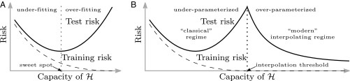
Fig. 1. Curves for training risk (dashed line) and test risk (solid line). (A) The classical U-shaped risk curve arising from the bias–variance trade-off. (B) The double-descent risk curve, which incorporates the U-shaped risk curve (i.e., the “classical” regime) together with the observed behavior from using high-capacity function classes (i.e., the “modern” interpolating regime), separated by the interpolation threshold. The predictors to the right of the interpolation threshold have zero training risk.
图 1|训练风险(虚线)和测试风险(实线)的曲线。(A) 由偏置–方差权衡得到的经典 U 形风险曲线。(B) 双下降风险曲线,它把 U 形风险曲线(即“经典”区间)与使用高容量函数类时所观察到的行为(即“现代”插值区间)合在一起,两者由插值阈值隔开。插值阈值右侧的预测器训练风险为零。
However, practitioners routinely use modern machine-learning methods, such as large neural networks and other nonlinear predictors that have very low or zero training risk. Despite the high function class capacity and near-perfect fit to training data, these predictors often give very accurate predictions on new data. Indeed, this behavior has guided a best practice in deep learning for choosing neural network architectures, specifically that the network should be large enough to permit effortless zero-loss training (called interpolation) of the training data (4). Moreover, in direct challenge to the bias–variance trade-off philosophy, recent empirical evidence indicates that neural networks and kernel machines trained to interpolate the training data obtain near-optimal test results even when the training data are corrupted with high levels of noise (5, 6).
然而,实践者日常使用的现代机器学习方法,例如大型神经网络以及其他非线性预测器,训练风险往往非常低,甚至为零。尽管函数类容量很高、对训练数据的拟合也近乎完美,这些预测器常常仍能在新数据上给出非常准确的预测。事实上,这一现象已经引导了深度学习中选择网络架构的一条最佳实践,即网络应当足够大,以便能够不费力地把训练数据的训练损失降到零(称为插值)(4)。此外,直接挑战偏置–方差权衡这一观念的是:近来的经验证据表明,即使训练数据被加上很高水平的噪声,训练到插值的神经网络和核机器仍能得到接近最优的测试结果(5, 6)。
The main finding of this work is a pattern in how performance on unseen data depends on model capacity and the mechanism underlying its emergence. This dependence, empirically witnessed with important model classes including neural networks and a range of datasets, is summarized in the “double-descent” risk curve shown in Fig. 1B. The curve subsumes the classical U-shaped risk curve from Fig. 1A by extending it beyond the point of interpolation.
本文的主要发现,是未见数据上的性能如何依赖于模型容量,以及这一规律出现的机制。这一依赖关系在包括神经网络在内的重要模型类以及一系列数据集上都可以经验地看到,概括为图 1B 所示的“双下降”风险曲线。这条曲线通过把经典的 U 形风险曲线延伸到插值点以外,把图 1A 中的曲线包含了进来。
When function class capacity is below the “interpolation threshold,” learned predictors exhibit the classical U-shaped curve from Fig. 1A. (In this paper, function class capacity is identified with the number of parameters needed to specify a function within the class.) The bottom of the U is achieved at the sweet spot which balances the fit to the training data and the susceptibility to overfitting: To the left of the sweet spot, predictors are underfitted, and immediately to the right, predictors are overfitted. When we increase the function class capacity high enough (e.g., by increasing the number of features or the size of the neural network architecture), the learned predictors achieve (near) perfect fits to the training data—i.e., interpolation. Although the learned predictors obtained at the interpolation threshold typically have high risk, we show that increasing the function class capacity beyond this point leads to decreasing risk, typically going below the risk achieved at the sweet spot in the “classical” regime.
当函数类容量低于“插值阈值”时,学到的预测器呈现出图 1A 中的经典 U 形曲线。(在本文中,函数类容量被等同于指定该类中一个函数所需的参数个数。)U 形的底部出现在平衡了对训练数据的拟合与对过拟合的敏感程度的甜区:甜区左侧的预测器欠拟合,紧靠右侧的预测器则过拟合。当把函数类容量提得足够高(例如通过增加特征数或增大神经网络架构)时,学到的预测器会对训练数据达到(近乎)完美的拟合,也就是插值。尽管在插值阈值处得到的预测器通常风险很高,我们表明,越过这一点继续增加函数类容量会导致风险下降,而且通常会降到低于“经典”区间里甜区所达到的风险。
All of the learned predictors to the right of the interpolation threshold fit the training data perfectly and have zero empirical risk. So why should some—in particular, those from richer functions classes—have lower test risk than others? The answer is that the capacity of the function class does not necessarily reflect how well the predictor matches the inductive bias appropriate for the problem at hand. For the learning problems we consider (a range of real-world datasets as well as synthetic data), the inductive bias that seems appropriate is the regularity or smoothness of a function as measured by a certain function space norm. Choosing the smoothest function that perfectly fits observed data is a form of Occam’s razor: The simplest explanation compatible with the observations should be preferred (cf. refs. 7 and 8). By considering larger function classes, which contain more candidate predictors compatible with the data, we are able to find interpolating functions that have smaller norm and are thus “simpler.” Thus, increasing function class capacity improves performance of classifiers.
插值阈值右侧的所有学到的预测器都完美拟合训练数据,经验风险为零。那么,为什么其中一些——尤其是来自更丰富函数类的那些——测试风险会比其他的更低?答案是:函数类的容量并不一定反映预测器与当前问题所适合的归纳偏置(inductive bias)匹配得有多好。对本文考虑的学习问题(一系列真实世界数据集以及合成数据)而言,看来合适的归纳偏置,是用某个函数空间范数来度量的函数正则性或平滑性。在完美拟合观测数据的函数中选择最平滑的那一个,是一种奥卡姆剃刀:应当优先选择与观测相容的最简单解释(参见文献 7 和 8)。通过考虑更大的函数类,其中包含更多与数据相容的候选预测器,我们就能够找到范数更小、因而更“简单”的插值函数。因此,增加函数类容量会改善分类器的性能。
Related ideas have been considered in the context of margins theory (7, 9, 10), where a larger function class may permit the discovery of a classifier with a larger margin. While the margins theory can be used to study classification, it does not apply to regression and also does not predict the second descent beyond the interpolation threshold. Recently, there has been an emerging recognition that certain interpolating predictors (not based on ERM) can indeed be provably statistically optimal or near optimal (11, 12), which is compatible with our empirical observations in the interpolating regime.
相关想法也曾在间隔理论(margins theory)的语境中被讨论过(7, 9, 10):更大的函数类 可能使人们发现间隔更大的分类器。间隔理论可以用来研究分类,但不适用于回归,也不能预测插值阈值之后的第二次下降。近来人们开始认识到,某些并非基于 ERM 的插值预测器确实可以在统计上被证明是最优或接近最优的(11, 12),这与我们在插值区间中的经验观察是相容的。
In the remainder of this article, we discuss empirical evidence for the double-descent curve and the mechanism for its emergence and conclude with some final observations and parting thoughts.
在本文的其余部分,我们讨论双下降曲线的经验证据及其出现机制,并在最后给出若干观察和结束语。
Neural Networks
神经网络
In this section, we discuss the double-descent risk curve in the context of neural networks.
本节讨论神经网络语境中的双下降风险曲线。
Random Fourier Features.
随机傅里叶特征。
We first consider a popular class of nonlinear parametric models called random Fourier features (RFF) (13), which can be viewed as a class of 2-layer neural networks with fixed weights in the first layer. The RFF model family with (complex-valued) parameters consists of functions of the form
我们首先考虑一类常用的非线性参数模型,称为随机傅里叶特征(random Fourier features,RFF)(13),它可以被看作第一层权重固定的两层神经网络。具有 个(复值)参数的 RFF 模型族 ,由如下形式的函数 组成
and the vectors are sampled independently from the standard normal distribution in . (We consider as a class of real-valued functions with real-valued parameters by taking real and imaginary parts separately.) Note that is a randomized function class, but as , the function class becomes a closer and closer approximation to the reproducing kernel Hilbert space (RKHS) corresponding to the Gaussian kernel, denoted by . While it is possible to directly use [e.g., as is done with kernel machines (14)], the random classes are computationally attractive to use when the sample size is large but the number of parameters is small compared with .
并且向量 是从 上的标准正态分布独立抽样得到的。(我们把实部和虚部分开处理,从而把 视为具有 个实值参数的实值函数类。)需要注意的是, 是随机的函数类,但当 时,这个函数类会越来越接近对应于高斯核的再生核希尔伯特空间(RKHS),记为 。虽然可以直接使用 [例如核机器所做的那样(14)],但当样本量 很大、而参数个数 相对于 较小时,随机类 在计算上更有吸引力。
Our learning procedure using is as follows. Given data from , we find the predictor via ERM with squared loss. That is, we minimize the empirical risk objective over all functions . When the minimizer is not unique (as is always the case when ), we choose the minimizer whose coefficients have the minimum norm. This choice of norm is intended as an approximation to the RKHS norm , which is generally difficult to compute for arbitrary functions in . For problems with multiple outputs (e.g., multiclass classification), we use functions with vector-valued outputs and the sum of the squared losses for each output.
我们使用 的学习程序如下。给定来自 的数据 ,我们用带平方损失的 ERM 在 中寻找预测器 。也就是说,在所有函数 上最小化经验风险目标 。当最小化器不唯一时(当 时总是如此),我们选择系数 具有最小 范数的那个最小化器。选择这一范数,是为了近似 RKHS 范数 ,而后者对 中的任意函数通常难以计算。对具有多个输出的问题(例如多类分类),我们使用向量值输出的函数,并把各个输出的平方损失加总。
In Fig. 2, we show the test risk of the predictors learned using on a subset of the popular dataset of handwritten digits called MNIST. Fig. 2 also shows the norm of the function coefficients, as well as the training risk. We see that for small values of , the test risk shows the classical U-shaped curve consistent with the bias–variance trade-off, with a peak occurring at the interpolation threshold . Some statistical analyses of RFF suggest choosing to obtain good test risk guarantees (15).
在图 2 中,我们展示了用 在流行的手写数字数据集 MNIST 的一个子集上学到的预测器的测试风险。图 2 还给出了函数系数的 范数以及训练风险。可以看到,当 较小时,测试风险呈现出与偏置–方差权衡一致的经典 U 形曲线,峰值出现在插值阈值 处。对 RFF 的一些统计分析建议取 ,以获得良好的测试风险保证(15)。
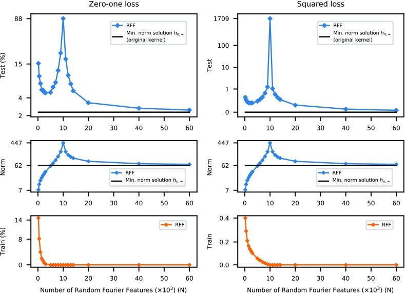
Fig. 2. Double-descent risk curve for the RFF model on MNIST. Shown are test risks (log scale), coefficient norms (log scale), and training risks of the RFF model predictors learned on a subset of MNIST (, 10 classes). The interpolation threshold is achieved at .
图 2|RFF 模型在 MNIST 上的双下降风险曲线。图中给出在 MNIST 一个子集(,10 类)上学到的 RFF 模型预测器 的测试风险(对数坐标)、系数 范数(对数坐标)以及训练风险。插值阈值在 处达到。
The interpolation regime connected with modern practice is shown to the right of the interpolation threshold, with . The model class that achieves interpolation with fewest parameters ( random features) yields the least accurate predictor. (In fact, it has no predictive ability for classification.) But as the number of features increases beyond , the accuracy improves dramatically, exceeding that of the predictor corresponding to the bottom of the U-shaped curve. The plot also shows that the predictor obtained from (the kernel machine) outperforms the predictors from for any finite .
与现代实践相联系的插值区间显示在插值阈值的右侧,此时 。以最少参数实现插值的模型类( 个随机特征)给出的预测器最不准确。(事实上,它对分类没有预测能力。)但当特征数增加到超过 时,精度会显著改善,并超过 U 形曲线底部所对应的预测器。图中还显示,由 (核机器)得到的预测器 ,其表现优于任何有限 下的 预测器。
What structural mechanisms account for the double-descent shape? When the number of features is much smaller than the sample size, , classical statistical arguments imply that the training risk is close to the test risk. Thus, for small , adding more features yields improvements in both the training and the test risks. However, as the number of features approaches (the interpolation threshold), features not present or only weakly present in the data are forced to fit the training data nearly perfectly. This results in classical overfitting as predicted by the bias–variance trade-off and prominently manifested at the peak of the curve, where the fit becomes exact.
怎样的结构机制可以说明双下降的形状?当特征数远小于样本量,即 时,经典的统计论证意味着训练风险接近测试风险。因此,对较小的 ,增加特征会同时改善训练风险和测试风险。然而,当特征数接近 (插值阈值)时,数据中并不存在或只微弱存在的特征被强制用来近乎完美地拟合训练数据。这导致偏置–方差权衡所预言的经典过拟合,并在曲线的峰值处突出表现出来,此时拟合变为精确拟合。
To the right of the interpolation threshold, all function classes are rich enough to achieve zero training risk. For the classes that we consider, there is no guarantee that the most regular, smallest norm predictor consistent with training data (namely , which is in ) is contained in the class for any finite . But increasing allows us to construct progressively better approximations to that smallest norm function. Thus, we expect to have learned predictors with largest norm at the interpolation threshold and for the norm of to decrease monotonically as increases, thus explaining the second descent segment of the curve. This is what we observe in Fig. 2, and indeed has better accuracy than all for any finite . Favoring small norm interpolating predictors turns out to be a powerful inductive bias on MNIST and other real and synthetic datasets (6). For noiseless data, we make this claim mathematically precise in SI Appendix.
在插值阈值右侧,所有函数类都丰富到足以把训练风险做到零。对本文考虑的类 而言,并不能保证与训练数据相容的最正则、最小范数预测器(也就是属于 的 )对任何有限的 都包含在 中。但增大 使我们能够逐步更好地逼近那个最小范数函数。因此,我们预期在插值阈值处学到的预测器范数最大,而 的范数会随着 增大而单调下降,从而解释曲线的第二段下降。这正是我们在图 2 中看到的,而且 的精度的确好于任何有限 下的 。偏好小范数插值预测器,在 MNIST 以及其他真实和合成数据集上被证明是一种有力的归纳偏置(6)。对无噪声数据,我们在《SI Appendix》中把这一论断写得在数学上更精确。
Additional empirical evidence for the same double-descent behavior using other datasets is presented in SI Appendix. For instance, we demonstrate double descent for rectified linear unit (ReLU) random feature models, a class of ReLU neural networks with a setting similar to that of RFF. We also describe a simple synthetic model, which can be regarded as a 1D version of the RFF model, where we observe the same double-descent behavior.
使用其他数据集得到的、同样支持双下降行为的额外经验证据见《SI Appendix》。例如,我们为修正线性单元(ReLU)随机特征模型展示了双下降,这是一类设定与 RFF 类似的 ReLU 神经网络。我们还描述了一个简单的合成模型,可以看作 RFF 模型的一维版本,在其中同样观察到了双下降行为。
Neural Networks and Backpropagation.
神经网络与反向传播。
In general multilayer neural networks (beyond RFF or ReLU random feature models), a learning algorithm will tune all of the weights to fit the training data, typically using versions of stochastic gradient descent (SGD), with backpropagation to compute partial derivatives. This flexibility increases the representational power of neural networks, but also makes ERM generally more difficult to implement. Nevertheless, as shown in Fig. 3, we observe that increasing the number of parameters in fully connected 2-layer neural networks leads to a risk curve qualitatively similar to that observed with RFF models. That the test risk improves beyond the interpolation threshold is compatible with the conjectured “small norm” inductive biases of the common training algorithms for neural networks (16, 17). We note that this transition from under- to overparameterized regimes for neural networks was also previously observed by refs. 18–21. In particular, ref. 21 draws a connection to the physical phenomenon of “jamming” in particle systems.
在一般的多层神经网络中(超出 RFF 或 ReLU 随机特征模型),学习算法会调整全部权重以拟合训练数据,通常使用随机梯度下降(SGD)的各种形式,并用反向传播计算偏导数。这种灵活性增加了神经网络的表示能力,但也使 ERM 一般来说更难实现。尽管如此,如图 3 所示,我们观察到,增加全连接两层神经网络的参数个数,会得到与 RFF 模型定性相似的风险曲线。测试风险在插值阈值之后仍会改善,这与关于神经网络常用训练算法具有“小范数”归纳偏置的猜想是相容的(16, 17)。我们注意到,神经网络从欠参数化到过参数化区间的这一转变,此前也由文献 18–21 观察到。尤其是文献 21,把它与粒子系统中的“堵塞”(jamming)物理现象联系起来。
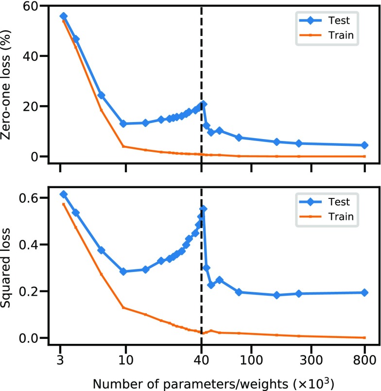
Fig. 3. Double-descent risk curve for a fully connected neural network on MNIST. Shown are training and test risks of a network with a single layer of hidden units, learned on a subset of MNIST (, , classes). The number of parameters is . The interpolation threshold (black dashed line) is observed at .
图 3|全连接神经网络在 MNIST 上的双下降风险曲线。图中给出在 MNIST 一个子集(,, 类)上学习的、具有单层 个隐单元的网络的训练风险和测试风险。参数个数为 。插值阈值(黑色虚线)出现在 处。
The computational complexity of ERM with neural networks makes the double-descent risk curve difficult to observe. Indeed, in the classical underparameterized regime (), the nonconvexity of the ERM optimization problem causes the behavior of local search-based heuristics, like SGD, to be highly sensitive to their initialization. Thus, if only suboptimal solutions are found for the ERM optimization problems, increasing the size of a neural network architecture may not always lead to a corresponding decrease in the training risk. This suboptimal behavior can lead to high variability in both the training and test risks that masks the double-descent curve.
神经网络上 ERM 的计算复杂性,使得双下降风险曲线不容易被观察到。事实上,在经典的欠参数化区间()里,ERM 优化问题的非凸性会使基于局部搜索的启发式方法(如 SGD)的行为对初始化高度敏感。因此,如果只找到了 ERM 优化问题的次优解,增大神经网络架构的规模未必总能带来训练风险的相应下降。这种次优行为会在训练风险和测试风险中造成很高的变异性,从而把双下降曲线掩盖掉。
It is common to use neural networks with an extremely large number of parameters (22). But to achieve interpolation for a single output (regression or 2-class classification) one expects to need at least as many parameters as there are data points. Moreover, if the prediction problem has more than one output (as in multiclass classification), then the number of parameters needed should be multiplied by the number of outputs. This is indeed the case empirically for neural networks shown in Fig. 3. Thus, for instance, datasets as large as ImageNet (23), which has examples and classes, may require networks with parameters to achieve interpolation; this is larger than many neural network models for ImageNet (22). In such cases, the classical regime of the U-shaped risk curve is more appropriate to understand generalization. For smaller datasets, these large neural networks would be firmly in the overparameterized regime, and simply training to obtain zero training risk often results in good test performance (5).
使用参数极多的神经网络是常见做法(22)。但要对单个输出(回归或两类分类)实现插值,人们预期至少需要与数据点数一样多的参数。而且,如果预测问题有不止一个输出(如多类分类),所需参数个数还应乘以输出个数。图 3 中的神经网络在经验上正是如此。因此,例如 ImageNet(23)这样约有 个样本、约 个类别的数据集,可能需要约 个参数的网络才能实现插值;这比许多用于 ImageNet 的神经网络模型都更大(22)。在这些情形里,用经典的 U 形风险曲线区间来理解泛化更为合适。对更小的数据集,这些大型神经网络会稳稳地处在过参数化区间,仅仅训练到训练风险为零,往往就能得到良好的测试表现(5)。
Additional results with neural networks are given in SI Appendix.
神经网络的其他结果见《SI Appendix》。
Decision Trees and Ensemble Methods
决策树与集成方法
Does the double-descent risk curve manifest with other prediction methods besides neural networks? We give empirical evidence that the families of functions explored by boosting with decision trees and random forests also show similar generalization behavior to that of neural nets, both before and after the interpolation threshold.
双下降风险曲线是否也会出现在神经网络以外的其他预测方法上?我们给出经验证据表明:用决策树做提升(boosting)以及随机森林所探索的函数族,在插值阈值之前和之后,都表现出与神经网络相似的泛化行为。
AdaBoost and random forests have recently been investigated in the interpolation regime by ref. 24 for classification. In particular, they give empirical evidence that, when AdaBoost and random forests are used with maximally large (interpolating) decision trees, the flexibility of the fitting methods yields interpolating predictors that are more robust to noise in the training data than the predictors produced by rigid, noninterpolating methods (e.g., AdaBoost or random forests with shallow trees). This in turn is said to yield better generalization. The averaging of the (near) interpolating trees ensures that the resulting function is substantially smoother than any individual tree, which aligns with an inductive bias that is compatible with many real-world problems.
文献 24 近来在分类的插值区间中考察了 AdaBoost 和随机森林。他们尤其给出经验证据表明:当 AdaBoost 和随机森林与尽可能大的(可插值的)决策树一起使用时,这些拟合方法的灵活性会产生比僵硬的非插值方法(例如使用浅树的 AdaBoost 或随机森林)对训练数据中的噪声更稳健的插值预测器,并进而被说成能带来更好的泛化。对(近乎)插值的树做平均,会确保得到的函数比任何单棵树都平滑得多,这与许多真实世界问题所适合的归纳偏置是一致的。
We can understand these flexible fitting methods in the context of the double-descent risk curve. Observe that the size of a decision tree (controlled by the number of leaves) is a natural way to parameterize the function class capacity: Trees with only 2 leaves correspond to 2-piecewise constant functions with an axis-aligned boundary, while trees with leaves can interpolate training examples. It is a classical observation that the U-shaped bias–variance trade-off curve manifests in many problems when the class capacity is considered this way (2). (The interpolation threshold may be reached with fewer than leaves in many cases, but is clearly an upper bound.) To further enlarge the function class, we consider ensembles (averages) of several interpolating trees.* So, beyond the interpolation threshold, we use the number of such trees to index the class capacity. When we view the risk curve as a function of class capacity defined in this hybrid fashion, we see the double-descent curve appear just as with neural networks (Fig. 4 and SI Appendix). We observe a similar phenomenon using boosting (26, 27), another popular ensemble method; the results are reported in SI Appendix.
我们可以在双下降风险曲线的语境中理解这些灵活的拟合方法。可以看到,决策树的规模(由叶子数控制)是参数化函数类容量的一种自然方式:只有 2 片叶子的树对应于边界与坐标轴对齐的两段常值函数,而有 片叶子的树可以插值 个训练样本。一个经典观察是:当这样来看待类容量时,许多问题上都会出现 U 形的偏置–方差权衡曲线(2)。(在许多情形里,插值阈值可能在少于 片叶子时就已经达到,但 显然是一个上界。)为了进一步扩大函数类,我们考虑若干棵插值树的集成(平均)。* 于是,在插值阈值之外,我们用这类树的数目来标记类容量。当我们把风险曲线看作以这种混合方式定义的类容量的函数时,就会像在神经网络中一样看到双下降曲线(图 4 及《SI Appendix》)。使用另一种流行的集成方法 提升(26, 27),我们也观察到类似现象;结果见《SI Appendix》。
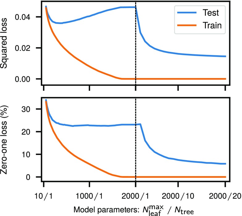
Fig. 4. Double-descent risk curve for random forests on MNIST. The double-descent risk curve is observed for random forests with increasing model complexity trained on a subset of MNIST (, 10 classes). Its complexity is controlled by the number of trees and the maximum number of leaves allowed for each tree .
图 4|随机森林在 MNIST 上的双下降风险曲线。在 MNIST 一个子集(,10 类)上训练、模型复杂度逐步增加的随机森林,表现出双下降风险曲线。其复杂度由树的数目 以及每棵树允许的最大叶子数 控制。
Concluding Thoughts
结语
The double-descent risk curve introduced in this paper reconciles the U-shaped curve predicted by the bias–variance trade-off and the observed behavior of rich models used in modern machine-learning practice. The posited mechanism that underlies its emergence is based on common inductive biases and hence can explain its appearance (and, we argue, ubiquity) in machine-learning applications.
本文引入的双下降风险曲线,调和了偏置–方差权衡所预言的 U 形曲线,与现代机器学习实践中所用丰富模型的观察行为。我们提出的、作为其出现基础的机制,建立在常见的归纳偏置之上,因而可以解释它在机器学习应用中的出现(以及,我们认为,它的普遍性)。
We conclude with some final remarks.
我们以若干最后的评论作结。
Historical Absence.
历史上为何少见。
The double-descent behavior may have been historically overlooked on account of several cultural and practical barriers. Observing the double-descent curve requires a parametric family of spaces with functions of arbitrary complexity. The linear settings studied extensively in classical statistics usually assume a small, fixed set of features and hence fixed fitting capacity. Richer families of function classes are typically used in the context of nonparametric statistics, where smoothing and regularization are almost always used (28). Regularization, of all forms, can both prevent interpolation and change the effective capacity of the function class, thus attenuating or masking the interpolation peak.
双下降行为在历史上可能由于若干文化和实践上的障碍而被忽视。要观察到双下降曲线,需要一个能够包含任意复杂度函数的参数化空间族。经典统计学中被广泛研究的线性设定,通常假定特征集合很小且固定,因而拟合容量也是固定的。更丰富的函数类通常出现在非参数统计中,而那里几乎总是使用平滑和正则化(28)。各种形式的正则化既可以阻止插值,也可以改变函数类的有效容量,从而减弱或掩盖插值峰值。
The RFF model is a popular and flexible parametric family. However, these models were originally proposed as a computationally favorable alternative to kernel machines. This computational advantage over traditional kernel methods holds only for , and hence models at or beyond the interpolation threshold are typically not considered.
RFF 模型是一类流行且灵活的参数族。不过,这些模型最初是作为核机器在计算上更有利的替代方案被提出的。相对传统核方法的这一计算优势仅在 时成立,因此位于或超过插值阈值的模型通常不被考虑。
The situation with general multilayer neural networks is slightly different and more involved. Due to the nonconvexity of the ERM optimization problem, solutions in the classical underparameterized regime are highly sensitive to initialization. Moreover, as we have seen, the peak at the interpolation threshold is observed within a narrow range of parameters. Sampling of the parameter space that misses that range may lead to the misleading impression that increasing the size of the network simply improves performance. Finally, in practice, training of neural networks is typically stopped as soon as (an estimate of) the test risk fails to improve. This early stopping has a strong regularizing effect that, as discussed above, makes it difficult to observe the interpolation peak.
一般多层神经网络的情况稍有不同,也更复杂。由于 ERM 优化问题的非凸性,经典欠参数化区间中的解对初始化高度敏感。此外,如我们已经看到的,插值阈值处的峰值只在很窄的参数范围内被观察到。对参数空间的抽样如果错过了这一范围,可能会造成一种误导性印象,即增大网络规模只会改善性能。最后,在实践中,神经网络的训练通常会在(对)测试风险(的估计)不再改善时立刻停止。这种早停具有很强的正则化效果,如上所述,会使得插值峰值难以被观察到。
Inductive Bias.
归纳偏置。
In this paper, we have dealt with several types of methods for choosing interpolating solutions. For random Fourier features, solutions are constructed explicitly by minimum norm linear regression in the feature space. As the number of features tends to infinity they approach the minimum functional norm solution in the reproducing kernel Hilbert space, a solution which maximizes functional smoothness subject to the interpolation constraints. For neural networks, the inductive bias owes to the specific training procedure used, which is typically SGD. When all but the final layer of the network are fixed (as in RFF models), SGD initialized at zero also converges to the minimum norm solution. While the behavior of SGD for more general neural networks is not fully understood, there is significant empirical and some theoretical evidence (e.g., ref. 16) that a similar minimum norm inductive bias is present. Yet another type of inductive bias related to averaging is used in random forests. Averaging potentially nonsmooth interpolating trees leads to an interpolating solution with a higher degree of smoothness; this averaged solution performs better than any individual interpolating tree.
在本文中,我们处理了若干类选择插值解的方法。对随机傅里叶特征,解是在特征空间中用最小范数线性回归显式构造的。当特征数趋于无穷时,它们会趋近再生核希尔伯特空间中的最小函数范数解,这个解在插值约束下使函数平滑性最大。对神经网络而言,归纳偏置来自所使用的具体训练程序,通常是 SGD。当网络除最后一层以外都被固定时(如在 RFF 模型中),从零初始化的 SGD 也会收敛到最小范数解。虽然更一般神经网络上 SGD 的行为尚未被完全理解,但已有大量经验证据和一些理论证据(例如文献 16)表明,类似的最小范数归纳偏置是存在的。随机森林中还使用了另一种与平均有关的归纳偏置。把可能并不平滑的插值树加以平均,会得到平滑程度更高的插值解;这个平均解的表现好于任何单棵插值树。
Remarkably, for kernel machines all 3 methods lead to the same minimum norm solution. Indeed, the minimum norm interpolating classifier, , can be obtained directly by explicit norm minimization (solving an explicit system of linear equations), through SGD, or by averaging trajectories of Gaussian processes [computing the posterior mean (29)].
值得注意的是,对核机器而言,这 3 种方法都会导向同一个最小范数解。事实上,最小范数插值分类器 既可以通过显式的范数最小化直接得到(求解一个显式的线性方程组),也可以通过 SGD 得到,还可以通过对高斯过程轨迹取平均得到[计算后验均值(29)]。
Optimization and Practical Considerations.
优化与实践上的考虑。
In our experiments, appropriately chosen “modern” models usually outperform the optimal classical model on the test set. But another important practical advantage of overparameterized models is in optimization. There is a growing understanding that larger models are “easy” to optimize as local methods, such as SGD, converge to global minima of the training risk in overparameterized regimes (e.g., ref. 30). Thus, large interpolating models can have low test risk and be easy to optimize at the same time, in particular with SGD (31). It is likely that the models to the left of the interpolation peak have optimization properties qualitatively different from those to the right, a distinction of significant practical import.
在我们的实验中,适当选择的“现代”模型通常在测试集上优于最优的经典模型。但过参数化模型的另一个重要实践优势在于优化。人们日益认识到,更大的模型“更容易”优化,因为在过参数化区间里,SGD 这类局部方法会收敛到训练风险的全局最小值(例如文献 30)。因此,大型插值模型可以同时具有较低的测试风险,并且——尤其是用 SGD 时——更容易优化(31)。插值峰值左侧的模型,其优化性质很可能与右侧有质的不同,这一区分具有重要的实践意义。
Outlook.
展望。
The classical U-shaped bias–variance trade-off curve has shaped our view of model selection and directed applications of learning algorithms in practice. The understanding of model performance developed in this work delineates the limits of classical analyses and opens additional lines of inquiry to study and compare computational, statistical, and mathematical properties of the classical and modern regimes in machine learning. We hope that this perspective, in turn, will help practitioners choose models and algorithms for optimal performance.
经典的 U 形偏置–方差权衡曲线,塑造了我们对模型选择的看法,并引导了学习算法在实践中的应用。本文所发展的对模型性能的理解,划出了经典分析的限度,并开辟了更多研究路径,去比较机器学习中经典区间与现代区间在计算、统计和数学上的性质。我们希望,这一视角反过来也能帮助实践者选择模型与算法,以获得最优性能。
Acknowledgments
致谢
M.B. was supported by NSF Grant RI-1815697. D.H. was supported by NSF Grant CCF-1740833 and a Sloan Research Fellowship.
M.B. 得到 NSF 基金 RI-1815697 的资助。D.H. 得到 NSF 基金 CCF-1740833 以及一项 Sloan Research Fellowship 的资助。
Footnotes
脚注
The authors declare no conflict of interest.
作者声明不存在利益冲突。
This article is a PNAS Direct Submission.
本文为 PNAS Direct Submission。
*These trees are trained in the way proposed in random forest except without bootstrap resampling. This is similar to the PERT method of ref. 25.
*这些树按随机森林中提出的方式训练,但不做自助法重抽样。这与文献 25 中的 PERT 方法类似。
This article contains supporting information online at www.pnas.org/lookup/suppl/doi:10.1073/pnas.1903070116/-/DCSupplemental.
References
参考文献
[1] Geman S., Bienenstock E., Doursat R., Neural networks and the bias/variance dilemma. Neural Comput. 4, 1–58 (1992).
[2] Hastie T., Tibshirani R., Friedman J., The Elements of Statistical Learning (Springer, 2001), vol. 1.
[3] Gigerenzer G., Brighton H., Homo heuristicus: Why biased minds make better inferences. Top. Cognit. Sci. 1, 107–143 (2009). [DOI] [PubMed]
[5] Zhang C., Bengio S., Hardt M., Recht B., Vinyals O., “Understanding deep learning requires rethinking generalization” in Proceedings of International Conference on Learning Representations (International Conference on Learning Representations, 2017).
[6] Belkin M., Ma S., Mandal S., “To understand deep learning we need to understand kernel learning” in Proceedings of the 35th International Conference on Machine Learning, Dy J., Krause A., Eds. (Proceedings of Machine Learning Research, Stockholm, Sweden 2018:), vol. 80, pp. 541–549.
[7] Vapnik V. N., The Nature of Statistical Learning Theory (Springer, 1995).
[8] Blumer A., Ehrenfeucht A., Haussler D., Warmuth M. K., Occam’s razor. Inf. Process. Lett. 24, 377–380 (1987).
[9] Bartlett P. L., The sample complexity of pattern classification with neural networks: The size of the weights is more important than the size of the network. IEEE Trans. Inf. Theory 44, 525–536 (1998).
[10] Schapire R. E., Freund Y., Bartlett P., Lee W. S., Boosting the margin: A new explanation for the effectiveness of voting methods. Ann. Stat. 26, 1651–1686 (1998).
[11] Belkin M., Hsu D., Mitra P., “Overfitting or perfect fitting? Risk bounds for classification and regression rules that interpolate” in Advances in Neural Information Processing Systems, Bengio S., Wallach H., Larochelle H., Grauman K., Cesa-Bianchi N., Garnett R., Eds. (Curran Associates, Inc., 2018), pp. 2300–2311.
[12] Belkin M., Rakhlin A., Tsybakov A. B., “Does data interpolation contradict statistical optimality?” in Proceedings of Machine Learning Research, K. Chaudhuri, M. Sugiyama, Eds. (Proceedings of Machine Learning Research, 2019), vol. 89, pp. 1611–1619.
[13] Rahimi A., Recht B., “Random features for large-scale kernel machines” in Advances in Neural Information Processing Systems, Platt J. C., Koller D., Singer Y., Roweis S. T., Eds. (Curran Associates, Inc., 2008), pp. 1177–1184.
[14] Boser B. E., Guyon I. M., Vapnik V. N., “A training algorithm for optimal margin classifiers” in Proceedings of the Fifth Annual Workshop on Computational Learning Theory (ACM, New York, NY, 1992), pp. 144–152.
[15] Rudi A., Rosasco L., “Generalization properties of learning with random features” in Advances in Neural Information Processing Systems, Guyon I., Luxburg U. V., Bengio S., Wallach H., Fergus R., Vishwanathan S., Garnett R., Eds. (Curran Associates, Inc., New York, NY, 2017), pp. 3215–3225.
[16] Gunasekar S., Woodworth B. E., Bhojanapalli S., Neyshabur B., Srebro N., “Implicit regularization in matrix factorization” in Advances in Neural Information Processing Systems, Guyon I., Luxburg U. V., Bengio S., Wallach H., Fergus R., Vishwanathan S., Garnett R., Eds. (Curran Associates, Inc., New York, NY, 2017), pp. 6151–6159.
[17] Li Y., Ma T., Zhang H., “Algorithmic regularization in over-parameterized matrix sensing and neural networks with quadratic activations” in Proceedings of the 31st Conference On Learning Theory, Bubeck S., Perchet V., Rigollet P., Eds. (Proceedings of Machine Learning Research, 2018;), vol. 75, pp. 2–47.
[18] Bös S., Opper M., “Dynamics of training” in Advances in Neural Information Processing Systems, Mozer M. C., Jordan M. I., Petsche T., Eds. (MIT Press, 1997), pp. 141–147.
[19] Advani M. S., Saxe A. M., High-dimensional dynamics of generalization error in neural networks. arXiv:1710.03667 (10 October 2017). [DOI] [PMC free article] [PubMed]
[20] Neal B., et al., A modern take on the bias-variance tradeoff in neural networks. arXiv:1810.08591 (25 January 2019).
[21] Spigler S., et al., A jamming transition from under-to over-parametrization affects loss landscape and generalization. arXiv:1810.09665 (22 October 2018).
[22] Canziani A., Paszke A., Culurciello E., An analysis of deep neural network models for practical applications. arXiv:1605.07678 (24 May 2016).
[23] Russakovsky O., et al., ImageNet large scale visual recognition challenge. Int. J. Comput. Vis. 115, 211–252 (2015).
[24] Wyner A. J., Olson M., Bleich J., Mease D., Explaining the success of adaboost and random forests as interpolating classifiers. J. Mach. Learn. Res. 18, 1–33(2017).
[25] Cutler A., Zhao G., Pert-perfect random tree ensembles. Comput. Sci. Stat. 33, 490–497 (2001).
[26] Friedman J. H., Greedy function approximation: A gradient boosting machine. Ann. Stat. 29, 1189–1232 (2001).
[27] Bühlmann P., Yu B., Boosting with the loss: Regression and classification. J. Am. Stat. Assoc. 98, 324–339 (2003).
[28] Wasserman L., All of Nonparametric Statistics (Springer, 2006).
[29] Rasmussen C. E., “Gaussian processes in machine learning” in Advanced Lectures on Machine Learning, Bousquet O., von Luxburg U., Rätsch G., Eds. (Springer, Berlin, 2004), pp. 63–71.
[30] Soltanolkotabi M., Javanmard A., Lee J. D., Theoretical insights into the optimization landscape of over-parameterized shallow neural networks. IEEE Trans. Inf. Theory 65, 742–769 (2018).
[31] Ma S., Bassily R., Belkin M., “The power of interpolation: Understanding the effectiveness of SGD in modern over-parametrized learning” in Proceedings of the 35th International Conference on Machine Learning, Proceedings of Machine Learning Research, Dy J., Krause A., eds. (PMLR, Stockholmsmässan, Stockholm, Sweden, 2018), vol. 80, pp. 3325–3334.