Off-Policy Deep Reinforcement Learning without Exploration
Off-Policy Deep Reinforcement Learning without Exploration
无需探索的离策略深度强化学习
Scott Fujimoto Affiliation: Department of Computer Science, McGill University, Montreal, Canada Affiliation: Mila Québec AI Institute Correspondence to: scott.fujimoto@mail.mcgill.ca David Meger Affiliation: Department of Computer Science, McGill University, Montreal, Canada Affiliation: Mila Québec AI Institute Doina Precup Affiliation: Department of Computer Science, McGill University, Montreal, Canada Affiliation: Mila Québec AI Institute
Off-Policy Deep Reinforcement Learning without Exploration: Supplementary Material
无需探索的离策略深度强化学习:补充材料
Scott Fujimoto Affiliation: Department of Computer Science, McGill University, Montreal, Canada Affiliation: Mila Québec AI Institute Correspondence to: scott.fujimoto@mail.mcgill.ca David Meger Affiliation: Department of Computer Science, McGill University, Montreal, Canada Affiliation: Mila Québec AI Institute Doina Precup Affiliation: Department of Computer Science, McGill University, Montreal, Canada Affiliation: Mila Québec AI Institute
Abstract
摘要
Many practical applications of reinforcement learning constrain agents to learn from a fixed batch of data which has already been gathered, without offering further possibility for data collection. In this paper, we demonstrate that due to errors introduced by extrapolation, standard off-policy deep reinforcement learning algorithms, such as DQN and DDPG, are incapable of learning without data correlated to the distribution under the current policy, making them ineffective for this fixed batch setting. We introduce a novel class of off-policy algorithms, batch-constrained reinforcement learning, which restricts the action space in order to force the agent towards behaving close to on-policy with respect to a subset of the given data. We present the first continuous control deep reinforcement learning algorithm which can learn effectively from arbitrary, fixed batch data, and empirically demonstrate the quality of its behavior in several tasks.
许多实际强化学习应用要求智能体只能从已经采集好的固定批次数据中学习,无法再继续采集。本文表明:由于外推引入的误差,标准离策略深度强化学习算法(如 DQN 与 DDPG)若缺少与当前策略分布相关的数据,就无法有效学习,因而在这种固定批次设定下失效。我们提出一类新的离策略算法——批次约束强化学习:通过限制动作空间,迫使智能体相对给定数据的某个子集表现得接近同策略。我们给出首个能从任意固定批次数据有效学习的连续控制深度强化学习算法,并在多项任务上实证展示其行为质量。
Keywords:
marginparsep has been altered. topmargin has been altered. marginparwidth has been altered. marginparpush has been altered.
关键词:
marginparsep has been altered. topmargin has been altered. marginparwidth has been altered. marginparpush has been altered.
The page layout violates the ICML style.
页面布局违反了 ICML 样式。
Please do not change the page layout, or include packages like geometry, savetrees, or fullpage, which change it for you.
请勿更改页面布局,也不要引入 geometry、savetrees 或 fullpage 等会替你改布局的宏包。
We’re not able to reliably undo arbitrary changes to the style. Please remove the offending package(s), or layout-changing commands and try again.
我们无法可靠地撤销对样式的任意改动。请移除相关宏包或改布局的命令后再试。
1 Introduction
1 引言
Batch reinforcement learning, the task of learning from a fixed dataset without further interactions with the environment, is a crucial requirement for scaling reinforcement learning to tasks where the data collection procedure is costly, risky, or time-consuming. Off-policy batch reinforcement learning has important implications for many practical applications. It is often preferable for data collection to be performed by some secondary controlled process, such as a human operator or a carefully monitored program. If assumptions on the quality of the behavioral policy can be made, imitation learning can be used to produce strong policies. However, most imitation learning algorithms are known to fail when exposed to suboptimal trajectories, or require further interactions with the environment to compensate (Hester et al. 2017; Sun et al. 2018; Cheng et al. 2018). On the other hand, batch reinforcement learning offers a mechanism for learning from a fixed dataset without restrictions on the quality of the data.
批次强化学习——在固定数据集上学习、不再与环境交互——是把强化学习扩展到数据采集昂贵、危险或耗时任务上的关键需求。离策略批次强化学习对许多实际应用有重要含义。数据采集往往更适合由某种受控的次级过程完成,例如人类操作员或受仔细监控的程序。若能对行为策略质量做假设,可用模仿学习得到强策略。但多数模仿学习算法在接触次优轨迹时会失败,或需要继续与环境交互来补偿(Hester et al. 2017;Sun et al. 2018;Cheng et al. 2018)。另一方面,批次强化学习提供了从固定数据集学习、且不对数据质量设限的机制。
Most modern off-policy deep reinforcement learning algorithms fall into the category of growing batch learning (Lange et al. 2012), in which data is collected and stored into an experience replay dataset (Lin 1992), which is used to train the agent before further data collection occurs. However, we find that these “off-policy” algorithms can fail in the batch setting, becoming unsuccessful if the dataset is uncorrelated to the true distribution under the current policy. Our most surprising result shows that off-policy agents perform dramatically worse than the behavioral agent when trained with the same algorithm on the same dataset.
多数现代离策略深度强化学习算法属于增长批次学习(Lange et al. 2012):数据被采集并存入经验回放数据集(Lin 1992),用于训练智能体后再继续采集。但我们发现这些「离策略」算法在批次设定下会失败——若数据集与当前策略下的真实分布不相关,就学不好。最令人惊讶的结果是:用同一算法、同一数据集训练时,离策略智能体的表现会大幅差于行为智能体。
This inability to learn truly off-policy is due to a fundamental problem with off-policy reinforcement learning we denote extrapolation**error, a phenomenon in which unseen state-action pairs are erroneously estimated to have unrealistic values. Extrapolation error can be attributed to a mismatch in the distribution of data induced by the policy and the distribution of data contained in the batch. As a result, it may be impossible to learn a value function for a policy which selects actions not contained in the batch.
这种无法真正离策略学习的原因,在于我们称为外推误差的离策略强化学习基本问题:未见过的状态–动作对被错误估计为不切实际的价值。外推误差可归因于策略诱导的数据分布与批次中数据分布的失配。因此,若策略选择的动作不在批次中,可能根本无法为其学到价值函数。
To overcome extrapolation error in off-policy learning, we introduce batch-constrained reinforcement learning, where agents are trained to maximize reward while minimizing the mismatch between the state-action visitation of the policy and the state-action pairs contained in the batch. Our deep reinforcement learning algorithm, Batch-Constrained deep Q-learning (BCQ), uses a state-conditioned generative model to produce only previously seen actions. This generative model is combined with a Q-network, to select the highest valued action which is similar to the data in the batch. Under mild assumptions, we prove this batch-constrained paradigm is necessary for unbiased value estimation from incomplete datasets for finite deterministic MDPs.
为克服离策略学习中的外推误差,我们引入批次约束强化学习:训练智能体最大化回报的同时,最小化策略的状态–动作访问与批次中状态–动作对之间的失配。我们的深度强化学习算法——批次约束深度 Q 学习(BCQ)——用状态条件生成模型只产生先前见过的动作。该生成模型与 Q 网络结合,选出与批次数据相似且价值最高的动作。在温和假设下,我们证明:对有限确定性 MDP,要从不完整数据集得到无偏价值估计,这种批次约束范式是必要的。
Unlike any previous continuous control deep reinforcement learning algorithms, BCQ is able to learn successfully without interacting with the environment by considering extrapolation error. Our algorithm is evaluated on a series of batch reinforcement learning tasks in MuJoCo environments (Todorov et al. 2012; Brockman et al. 2016), where extrapolation error is particularly problematic due to the high-dimensional continuous action space, which is impossible to sample exhaustively. Our algorithm offers a unified view on imitation and off-policy learning, and is capable of learning from purely expert demonstrations, as well as from finite batches of suboptimal data, without further exploration. We remark that BCQ is only one way to approach batch-constrained reinforcement learning in a deep setting, and we hope that it will be serve as a foundation for future algorithms. To ensure reproducibility, we provide precise experimental and implementation details, and our code is made available (https://github.com/sfujim/BCQ).
与以往任何连续控制深度强化学习算法不同,BCQ 通过考虑外推误差,无需与环境交互即可成功学习。算法在 MuJoCo 环境(Todorov et al. 2012;Brockman et al. 2016)的一系列批次强化学习任务上评测;高维连续动作空间无法穷尽采样,外推误差在此尤为严重。我们的算法统一了模仿学习与离策略学习的视角,既能从纯专家示范学习,也能从有限批次的次优数据学习,而无需继续探索。需要指出,BCQ 只是深度设定下实现批次约束强化学习的一种方式,我们希望它能成为未来算法的基础。为确保可复现,我们提供精确实验与实现细节,并公开代码(https://github.com/sfujim/BCQ)。
2 Background
2 背景
In reinforcement learning, an agent interacts with its environment, typically assumed to be a Markov decision process (MDP) , with state space , action space , and transition dynamics . At each discrete time step, the agent receives a reward for performing action in state and arriving at the state . The goal of the agent is to maximize the expectation of the sum of discounted rewards, known as the return , which weighs future rewards with respect to the discount factor .
强化学习中,智能体与环境交互;环境通常假设为马尔可夫决策过程(MDP),含状态空间 、动作空间 与转移动力学 。在每个离散时间步,智能体在状态 执行动作 并到达 时获得奖励 。目标是最大化折扣奖励之和的期望,即回报 ,其中未来奖励由折扣因子 加权。
The agent selects actions with respect to a policy , which exhibits a distribution over the states visited by the policy. Each policy has a corresponding value function , the expected return when following the policy after taking action in state . For a given policy , the value function can be computed through the Bellman operator :
智能体按策略 选动作;该策略在其访问的状态 上诱导分布 。每个策略 对应价值函数 ,即在状态 采取动作 后再遵循该策略的期望回报。对给定策略 ,价值函数可通过 Bellman 算子 计算:
The Bellman operator is a contraction for with unique fixed point (Bertsekas & Tsitsiklis 1996). is known as the optimal value function, which has a corresponding optimal policy obtained through greedy action choices. For large or continuous state and action spaces, the value can be approximated with neural networks, e.g. using the Deep Q-Network algorithm (DQN) (Mnih et al. 2015). In DQN, the value function is updated using the target:
对 ,Bellman 算子是压缩映射,有唯一不动点 (Bertsekas & Tsitsiklis 1996)。 称为最优价值函数,对应通过贪婪选动作得到的最优策略。对大或连续的状态与动作空间,可用神经网络近似价值,例如 Deep Q-Network 算法(DQN)(Mnih et al. 2015)。在 DQN 中,价值函数 用如下目标更新:
Q-learning is an off-policy algorithm (Sutton & Barto 1998), meaning the target can be computed without consideration of how the experience was generated. In principle, off-policy reinforcement learning algorithms are able to learn from data collected by any behavioral policy. Typically, the loss is minimized over mini-batches of tuples of the agent’s past data, , sampled from an experience replay dataset (Lin 1992). For shorthand, we often write if there exists a transition tuple containing in the batch , and similarly for or . In batch reinforcement learning, we assume is fixed and no further interaction with the environment occurs. To further stabilize learning, a target network with frozen parameters , is used in the learning target. The parameters of the target network are updated to the current network parameters after a fixed number of time steps, or by averaging for some small (Lillicrap et al. 2015).
Q-learning 是离策略算法(Sutton & Barto 1998),意味着计算目标时无需考虑经验如何产生。原则上,离策略强化学习算法可从任意行为策略采集的数据中学习。通常,损失在智能体历史数据的小批次元组 上最小化,这些元组从经验回放数据集 (Lin 1992)中采样。为简写,若批次 中存在含 的转移元组,则写 ;对 或 同理。在批次强化学习中,我们假设 固定且不再与环境交互。为进一步稳定学习,学习目标中使用参数冻结的目标网络 。目标网络参数 在固定步数后更新为当前网络参数 ,或以小 做平均 (Lillicrap et al. 2015)。
In a continuous action space, the analytic maximum of Equation (2) is intractable. In this case, actor-critic methods are commonly used, where action selection is performed through a separate policy network , known as the actor, and updated with respect to a value estimate, known as the critic (Sutton & Barto 1998; Konda & Tsitsiklis 2003). This policy can be updated following the deterministic policy gradient theorem (Silver et al. 2014):
在连续动作空间中,公式 (2) 的解析最大值不可求。此时常用 actor-critic:由独立的策略网络 (actor)选动作,并相对价值估计(critic)更新(Sutton & Barto 1998;Konda & Tsitsiklis 2003)。该策略可按确定性策略梯度定理(Silver et al. 2014)更新:
which corresponds to learning an approximation to the maximum of , by propagating the gradient through both and . When combined with off-policy deep Q-learning to learn , this algorithm is referred to as Deep Deterministic Policy Gradients (DDPG) (Lillicrap et al. 2015).
这对应于通过把梯度同时经 与 回传,学习对 最大值的近似。与用离策略深度 Q 学习来学 相结合时,该算法称为深度确定性策略梯度(DDPG)(Lillicrap et al. 2015)。
3 Extrapolation Error
3 外推误差
Extrapolation error is an error in off-policy value learning which is introduced by the mismatch between the dataset and true state-action visitation of the current policy. The value estimate is affected by extrapolation error during a value update where the target policy selects an unfamiliar action at the next state in the backed-up value estimate, such that is unlikely, or not contained, in the dataset. The cause of extrapolation error can be attributed to several related factors:
外推误差是离策略价值学习中的误差,由数据集与当前策略真实状态–动作访问之间的失配引入。当价值更新时,目标策略在下一状态 选出不熟悉的动作 ,使备份价值估计中的 在数据集中不太可能出现或不存在,则 会受外推误差影响。外推误差的成因可归为若干相关因素:
Absent Data. If any state-action pair is unavailable, then error is introduced as some function of the amount of similar data and approximation error. This means that the estimate of may be arbitrarily bad without sufficient data near .
数据缺失。 若任一状态–动作对 不可用,则误差是相似数据量与逼近误差的某种函数。这意味着若 附近数据不足, 的估计可能任意差。
Model Bias. When performing off-policy Q-learning with a batch , the Bellman operator is approximated by sampling transitions tuples from to estimate the expectation over . However, for a stochastic MDP, without infinite state-action visitation, this produces a biased estimate of the transition dynamics:
模型偏差。 用批次 做离策略 Q 学习时,Bellman 算子 通过从 采样转移元组 来近似对 的期望。但对随机 MDP,若没有无穷的状态–动作访问,这会对转移动力学产生有偏估计:
where the expectation is with respect to transitions in the batch , rather than the true MDP.
其中期望相对批次 中的转移,而非真实 MDP。
Training Mismatch. Even with sufficient data, in deep Q-learning systems, transitions are sampled uniformly from the dataset, giving a loss weighted with respect to the likelihood of data in the batch:
训练失配。 即便数据充足,在深度 Q 学习系统中,转移从数据集均匀采样,损失按批次中数据的似然加权:
If the distribution of data in the batch does not correspond with the distribution under the current policy, the value function may be a poor estimate of actions selected by the current policy, due to the mismatch in training.
若批次中数据分布与当前策略下的分布不一致,由于训练失配,价值函数可能对当前策略所选动作给出很差的估计。
We remark that re-weighting the loss in Equation (5) with respect to the likelihood under the current policy can still result in poor estimates if state-action pairs with high likelihood under the current policy are not found in the batch. This means only a subset of possible policies can be evaluated accurately. As a result, learning a value estimate with off-policy data can result in large amounts of extrapolation error if the policy selects actions which are not similar to the data found in the batch. In the following section, we discuss how state of the art off-policy deep reinforcement learning algorithms fail to address the concern of extrapolation error, and demonstrate the implications in practical examples.
需要指出:即便把公式 (5) 的损失按当前策略下的似然重加权,若当前策略下高似然的状态–动作对不在批次中,估计仍可能很差。这意味着只有一部分可能策略能被准确评估。因此,用离策略数据学习价值估计时,若策略选择与批次数据不相似的动作,可能产生大量外推误差。下一节讨论当前最先进的离策略深度强化学习算法如何未能解决外推误差,并在实际例子中展示其影响。
3.1 Extrapolation Error in Deep Reinforcement Learning
3.1 深度强化学习中的外推误差
Deep Q-learning algorithms (Mnih et al. 2015) have been labeled as off-policy due to their connection to off-policy Q-learning (Watkins 1989). However, these algorithms tend to use near-on-policy exploratory policies, such as -greedy, in conjunction with a replay buffer (Lin 1992). As a result, the generated dataset tends to be heavily correlated to the current policy. In this section, we examine how these off-policy algorithms perform when learning with uncorrelated datasets. Our results demonstrate that the performance of a state of the art deep actor-critic algorithm, DDPG (Lillicrap et al. 2015), deteriorates rapidly when the data is uncorrelated and the value estimate produced by the deep Q-network diverges. These results suggest that off-policy deep reinforcement learning algorithms are ineffective when learning truly off-policy.
深度 Q 学习算法(Mnih et al. 2015)因其与离策略 Q-learning(Watkins 1989)的联系而被标为离策略。但这些算法往往配合回放缓冲使用近同策略的探索策略,如 -greedy(Lin 1992)。因此生成的数据集往往与当前策略高度相关。本节考察这些离策略算法在不相关数据集上学习时的表现。结果表明:当前先进的深度 actor-critic 算法 DDPG(Lillicrap et al. 2015)在数据不相关时表现迅速恶化,深度 Q 网络产生的价值估计发散。这些结果说明,离策略深度强化学习算法在真正离策略学习时是无效的。
Our practical experiments examine three different batch settings in OpenAI gym’s Hopper-v1 environment (Todorov et al. 2012; Brockman et al. 2016), which we use to train an off-policy DDPG agent with no interaction with the environment. Experiments with additional environments and specific details can be found in the Supplementary Material.
实际实验在 OpenAI gym 的 Hopper-v1 环境(Todorov et al. 2012;Brockman et al. 2016)上考察三种批次设定,用其训练离策略 DDPG 智能体且不与环境交互。更多环境与具体细节见补充材料。
(a) Final buffer performance
Batch 1 (Final buffer). We train a DDPG agent for 1 million time steps, adding Gaussian noise to actions for high exploration, and store all experienced transitions. This collection procedure creates a dataset with a diverse set of states and actions, with the aim of sufficient coverage.
批次 1(最终缓冲)。 训练一个 DDPG 智能体 100 万步,对动作加 高斯噪声以增强探索,并存储全部经历的转移。该采集过程旨在得到状态与动作多样、覆盖充分的数据集。
Batch 2 (Concurrent). We concurrently train the off-policy and behavioral DDPG agents, for 1 million time steps. To ensure sufficient exploration, a standard Gaussian noise is added to actions taken by the behavioral policy. Each transition experienced by the behavioral policy is stored in a buffer replay, which both agents learn from. As a result, both agents are trained with the identical dataset.
批次 2(并发)。 同时训练离策略与行为 DDPG 智能体共 100 万步。为保证充分探索,行为策略动作加标准 高斯噪声。行为策略经历的每次转移存入回放缓冲,两个智能体都从中学习。因此两者用同一数据集训练。
Batch 3 (Imitation). A trained DDPG agent acts as an expert, and is used to collect a dataset of 1 million transitions.
批次 3(模仿)。 训练好的 DDPG 智能体充当专家,采集 100 万次转移的数据集。
In Figure 1, we graph the performance of the agents as they train with each batch, as well as their value estimates. Straight lines represent the average return of episodes contained in the batch. Additionally, we graph the learning performance of the behavioral agent for the relevant tasks.
在图 1 中,我们绘制各批次训练过程中智能体的表现及其价值估计。直线表示批次中所含回合的平均回报。此外还绘制相关任务上行为智能体的学习曲线。
Our experiments demonstrate several surprising facts about off-policy deep reinforcement learning agents. In each task, the off-policy agent performances significantly worse than the behavioral agent. Even in the concurrent experiment, where both agents are trained with the same dataset, there is a large gap in performance in every single trial. This result suggests that differences in the state distribution under the initial policies is enough for extrapolation error to drastically offset the performance of the off-policy agent. Additionally, the corresponding value estimate exhibits divergent behavior, while the value estimate of the behavioral agent is highly stable. In the final buffer experiment, the off-policy agent is provided with a large and diverse dataset, with the aim of providing sufficient coverage of the initial policy. Even in this instance, the value estimate is highly unstable, and the performance suffers. In the imitation setting, the agent is provided with expert data. However, the agent quickly learns to take non-expert actions, under the guise of optimistic extrapolation. As a result, the value estimates rapidly diverge and the agent fails to learn.
实验揭示了关于离策略深度强化学习智能体的若干令人惊讶的事实。在每项任务上,离策略智能体都显著差于行为智能体。即便在并发实验中两者用同一数据集训练,每次试验仍有很大表现差距。这表明初始策略下状态分布的差异就足以让外推误差大幅抵消离策略智能体的表现。同时,对应的价值估计呈现发散行为,而行为智能体的价值估计高度稳定。在最终缓冲实验中,离策略智能体得到大而多样的数据集,本意是充分覆盖初始策略;即便如此,价值估计仍高度不稳,表现受损。在模仿设定中,智能体得到专家数据,却很快在乐观外推的假象下学会采取非专家动作,价值估计迅速发散,学习失败。
Although extrapolation error is not necessarily positively biased, when combined with maximization in reinforcement learning algorithms, extrapolation error provides a source of noise that can induce a persistent overestimation bias (Thrun & Schwartz 1993; Van Hasselt et al. 2016; Fujimoto et al. 2018). In an on-policy setting, extrapolation error may be a source of beneficial exploration through an implicit “optimism in the face of uncertainty” strategy (Lai & Robbins 1985; Jaksch et al. 2010). In this case, if the value function overestimates an unknown state-action pair, the policy will collect data in the region of uncertainty, and the value estimate will be corrected. However, when learning off-policy, or in a batch setting, extrapolation error will never be corrected due to the inability to collect new data.
尽管外推误差未必带正偏,但与强化学习算法中的最大化结合时,它会成为噪声源,诱发持续的高估偏差(Thrun & Schwartz 1993;Van Hasselt et al. 2016;Fujimoto et al. 2018)。在同策略设定下,外推误差可能通过隐式「面对不确定性时乐观」策略成为有益探索(Lai & Robbins 1985;Jaksch et al. 2010):若价值函数高估未知状态–动作对,策略会在不确定区域采集数据,价值估计得到校正。但在离策略或批次设定下,因无法采集新数据,外推误差永远得不到校正。
These experiments show extrapolation error can be highly detrimental to learning off-policy in a batch reinforcement learning setting. While the continuous state space and multi-dimensional action space in MuJoCo environments are contributing factors to extrapolation error, the scale of these tasks is small compared to real world settings. As a result, even with a sufficient amount of data collection, extrapolation error may still occur due to the concern of catastrophic forgetting (McCloskey & Cohen 1989; Goodfellow et al. 2013). Consequently, off-policy reinforcement learning algorithms used in the real-world will require practical guarantees without exhaustive amounts of data.
这些实验表明,外推误差对批次强化学习设定下的离策略学习极为有害。MuJoCo 环境的连续状态空间与多维动作空间虽是外推误差的促成因素,但这些任务的规模相对真实世界仍偏小。因此,即便采集了足够数据,仍可能因灾难性遗忘(McCloskey & Cohen 1989;Goodfellow et al. 2013)出现外推误差。结果是,用于真实世界的离策略强化学习算法需要在不依赖穷尽数据量的前提下给出实用保证。
4 Batch-Constrained Reinforcement Learning
4 批次约束强化学习
Current off-policy deep reinforcement learning algorithms fail to address extrapolation error by selecting actions with respect to a learned value estimate, without consideration of the accuracy of the estimate. As a result, certain out-of-distribution actions can be erroneously extrapolated to higher values. However, the value of an off-policy agent can be accurately evaluated in regions where data is available. We propose a conceptually simple idea: to avoid extrapolation error a policy should induce a similar state-action visitation to the batch. We denote policies which satisfy this notion as batch-constrained. To optimize off-policy learning for a given batch, batch-constrained policies are trained to select actions with respect to three objectives:
当前离策略深度强化学习算法按学到的价值估计选动作,不考虑估计是否准确,因而未能解决外推误差。结果是某些分布外动作会被错误外推到更高价值。但在有数据的区域,离策略智能体的价值可以被准确评估。我们提出一个概念上简单的想法:为避免外推误差,策略应诱导与批次相似的状态–动作访问。满足这一概念的策略称为批次约束策略。为对给定批次优化离策略学习,批次约束策略按三个目标选动作:
(1) Minimize the distance of selected actions to the data in the batch.
(1) 最小化所选动作与批次数据之间的距离。
(2) Lead to states where familiar data can be observed.
(2) 导向可观察到熟悉数据的状态。
(3) Maximize the value function.
(3) 最大化价值函数。
We note the importance of objective (1) above the others, as the value function and estimates of future states may be arbitrarily poor without access to the corresponding transitions. That is, we cannot correctly estimate (2) and (3) unless (1) is sufficiently satisfied. As a result, we propose optimizing the value function, along with some measure of future certainty, with a constraint limiting the distance of selected actions to the batch. This is achieved in our deep reinforcement learning algorithm through a state-conditioned generative model, to produce likely actions under the batch. This generative model is combined with a network which aims to optimally perturb the generated actions in a small range, along with a Q-network, used to select the highest valued action. Finally, we train a pair of Q-networks, and take the minimum of their estimates during the value update. This update penalizes states which are unfamiliar, and pushes the policy to select actions which lead to certain data.
我们强调目标 (1) 相对其他目标的重要性:若无法访问相应转移,价值函数与未来状态估计可能任意差。也就是说,除非 (1) 被充分满足,否则无法正确估计 (2) 与 (3)。因此,我们建议在限制所选动作到批次距离的约束下,优化价值函数以及某种未来确定性度量。深度强化学习算法通过状态条件生成模型实现这一点,以产生批次下似然高的动作。该生成模型与一个旨在小范围内最优扰动生成动作的网络、以及用于选出最高价值动作的 Q 网络相结合。最后,我们训练一对 Q 网络,并在价值更新时取它们估计的最小值。该更新惩罚不熟悉的状态,并推动策略选择导向确定数据的动作。
We begin by analyzing the theoretical properties of batch-constrained policies in a finite MDP setting, where we are able to quantify extrapolation error precisely. We then introduce our deep reinforcement learning algorithm in detail, Batch-Constrained deep Q-learning (BCQ) by drawing inspiration from the tabular analogue.
我们先在有限 MDP 设定下分析批次约束策略的理论性质,以便精确量化外推误差。随后详细介绍受表格情形启发的深度强化学习算法——批次约束深度 Q 学习(BCQ)。
4.1 Addressing Extrapolation Error in Finite MDPs
4.1 在有限 MDP 中应对外推误差
In the finite MDP setting, extrapolation error can be described by the bias from the mismatch between the transitions contained in the buffer and the true MDP. We find that by inducing a data distribution that is contained entirely within the batch, batch-constrained policies can eliminate extrapolation error entirely for deterministic MDPs. In addition, we show that the batch-constrained variant of Q-learning converges to the optimal policy under the same conditions as the standard form of Q-learning. Moreover, we prove that for a deterministic MDP, batch-constrained Q-learning is guaranteed to match, or outperform, the behavioral policy when starting from any state contained in the batch. All of the proofs for this section can be found in the Supplementary Material.
在有限 MDP 设定下,外推误差可由缓冲中所含转移与真实 MDP 之间的偏差来描述。我们发现:通过诱导完全包含在批次内的数据分布,批次约束策略可对确定性 MDP 完全消除外推误差。此外,我们证明批次约束版 Q-learning 在与标准 Q-learning 相同的条件下收敛到最优策略。更进一步,我们证明:对确定性 MDP,从批次中任一状态出发,批次约束 Q-learning 保证匹配或超过行为策略。本节全部证明见补充材料。
A value estimate can be learned using an experience replay buffer . This involves sampling transition tuples with uniform probability, and applying the temporal difference update (Sutton 1988; Watkins 1989):
可用经验回放缓冲 学习价值估计 。做法是以均匀概率采样转移元组 ,并应用时序差分更新(Sutton 1988;Watkins 1989):
If , this is known as Q-learning. Assuming a non-zero probability of sampling any possible transition tuple from the buffer and infinite updates, Q-learning converges to the optimal value function.
若 ,即 Q-learning。假设能以非零概率从缓冲采样任意可能转移元组且更新无穷多次,则 Q-learning 收敛到最优价值函数。
We begin by showing that the value function learned with the batch corresponds to the value function for an alternate MDP . From the true MDP and initial values , we define the new MDP with the same action and state space as , along with an additional terminal state . has transition probabilities , where is the number of times the tuple is observed in . If , then , where is set to the initialized value of .
我们首先证明:用批次 学到的价值函数 对应于另一 MDP 的价值函数。从真实 MDP 与初始值 出发,定义新 MDP :动作与状态空间与 相同,并额外增加终止状态 。 的转移概率为 ,其中 是元组 在 中出现的次数。若 ,则 ,并把 设为 的初始化值。
Theorem 1. Performing Q-learning by sampling from a batch converges to the optimal value function under the MDP .
定理 1。 通过从批次 采样做 Q-learning,收敛到 MDP 下的最优价值函数。
We define as the tabular extrapolation error, which accounts for the discrepancy between the value function computed with the batch and the value function computed with the true MDP :
我们将 定义为表格外推误差,用以刻画用批次 计算的价值函数 与用真实 MDP 计算的价值函数 之间的差异:
For any policy , the exact form of can be computed through a Bellman-like equation:
对任意策略 , 的精确形式可通过类 Bellman 方程计算:
$$\begin{split}\epsilon_{\text{MDP}}(s,a)~&=\sum_{s^{\prime}}\left(p_{M}(s^{\prime}|s,a)-p_{\mathcal{B}}(s^{\prime}|s,a)\right)\
&\left(r(s,a,s^{\prime})+\gamma\sum_{a^{\prime}}\pi(a^{\prime}|s^{\prime})Q^{\pi}{\mathcal{B}}(s^{\prime},a^{\prime})\right)\
&+p{M}(s^{\prime}|s,a)\gamma\sum_{a^{\prime}}\pi(a^{\prime}|s^{\prime})\epsilon_{\text{MDP}}(s^{\prime},a^{\prime}).\end{split} \tag{8}$$
This means extrapolation error is a function of divergence in the transition distributions, weighted by value, along with the error at succeeding states. If the policy is chosen carefully, the error between value functions can be minimized by visiting regions where the transition distributions are similar. For simplicity, we denote
这意味着外推误差是转移分布差异(按价值加权)以及后续状态误差的函数。若谨慎选择策略,可通过访问转移分布相近的区域来最小化价值函数之间的误差。为简便,记
To evaluate a policy exactly at relevant state-action pairs, only is required. We can then determine the condition required to evaluate the exact expected return of a policy without extrapolation error.
要在相关状态–动作对上精确评估策略 ,只需 。由此可确定在无外推误差下精确评估策略期望回报所需的条件。
Lemma 1. For all reward functions, if and only if for all and such that and .
引理 1。 对所有奖励函数, 当且仅当对所有满足 且 的 以及所有 ,有 。
Lemma 1 states that if and exhibit the same transition probabilities in regions of relevance, the policy can be accurately evaluated. For a stochastic MDP this may require an infinite number of samples to converge to the true distribution, however, for a deterministic MDP this requires only a single transition. This means a policy which only traverses transitions contained in the batch, can be evaluated without error. More formally, we denote a policy as batch-constrained if for all where and then . Additionally, we define a batch as coherent if for all then unless is a terminal state. This condition is trivially satisfied if the data is collected in trajectories, or if all possible states are contained in the batch. With a coherent batch, we can guarantee the existence of a batch-constrained policy.
引理 1 表明:若 与 在相关区域展现相同转移概率,则策略可被准确评估。对随机 MDP,这可能需要无穷多样本才能收敛到真实分布;但对确定性 MDP,只需单次转移。这意味着只遍历批次中所含转移的策略可无误差评估。更形式地,若对所有满足 且 的 都有 ,则称策略 为批次约束。此外,若对所有 ,除非 为终止状态否则 ,则称批次 为连贯。若数据按轨迹采集,或批次包含全部可能状态,该条件平凡满足。有了连贯批次,即可保证批次约束策略存在。
Theorem 2. For a deterministic MDP and all reward functions, if and only if the policy is batch-constrained. Furthermore, if is coherent, then such a policy must exist if the start state .
定理 2。 对确定性 MDP 与所有奖励函数, 当且仅当策略 是批次约束的。此外,若 连贯,且起始状态 ,则这样的策略必然存在。
Batch-constrained policies can be used in conjunction with Q-learning to form batch-constrained Q-learning (BCQL), which follows the standard tabular Q-learning update while constraining the possible actions with respect to the batch:
批次约束策略可与 Q-learning 结合形成批次约束 Q-learning(BCQL):遵循标准表格 Q-learning 更新,同时按批次约束可能动作:
BCQL converges under the same conditions as the standard form of Q-learning, noting the batch-constraint is nonrestrictive given infinite state-action visitation.
BCQL 在与标准 Q-learning 相同的条件下收敛;注意在无穷状态–动作访问下,批次约束并无限制性。
Theorem 3. Given the Robbins-Monro stochastic convergence conditions on the learning rate , and standard sampling requirements from the environment, BCQL converges to the optimal value function $Q^{}$.*
定理 3。 给定学习率 的 Robbins-Monro 随机收敛条件,以及环境的标准采样要求,BCQL 收敛到最优价值函数 $Q^{}$。*
The more interesting property of BCQL is that for a deterministic MDP and any coherent batch , BCQL converges to the optimal batch-constrained policy such that for all and .
BCQL 更有趣的性质是:对确定性 MDP 与任意连贯批次 ,BCQL 收敛到最优批次约束策略 ,使得对所有 与 ,有 。
Theorem 4. Given a deterministic MDP and coherent batch , along with the Robbins-Monro stochastic convergence conditions on the learning rate and standard sampling requirements on the batch , BCQL converges to where $\pi^{}(s)=\argmax_{a\text{ s.t.}(s,a)\in\mathcal{B}}Q^{\pi}_{\mathcal{B}}(s,a)$ is the optimal batch-constrained policy.*
定理 4。 给定确定性 MDP 与连贯批次 ,以及学习率 的 Robbins-Monro 随机收敛条件与对批次 的标准采样要求,BCQL 收敛到 ,其中 $\pi^{}(s)=\argmax_{a\text{ s.t.}(s,a)\in\mathcal{B}}Q^{\pi}_{\mathcal{B}}(s,a)$ 是最优批次约束策略。*
This means that BCQL is guaranteed to outperform any behavioral policy when starting from any state contained in the batch, effectively outperforming imitation learning. Unlike standard Q-learning, there is no condition on state-action visitation, other than coherency in the batch.
这意味着从批次中任一状态出发,BCQL 保证超过任意行为策略,从而有效优于模仿学习。与标准 Q-learning 不同,除批次连贯性外,对状态–动作访问没有其他条件。
4.2 Batch-Constrained Deep Reinforcement Learning
4.2 批次约束深度强化学习
We introduce our approach to off-policy batch reinforcement learning, Batch-Constrained deep Q-learning (BCQ). BCQ approaches the notion of batch-constrained through a generative model. For a given state, BCQ generates plausible candidate actions with high similarity to the batch, and then selects the highest valued action through a learned Q-network. Furthermore, we bias this value estimate to penalize rare, or unseen, states through a modification to Clipped Double Q-learning (Fujimoto et al. 2018). As a result, BCQ learns a policy with a similar state-action visitation to the data in the batch, as inspired by the theoretical benefits of its tabular counterpart.
我们提出离策略批次强化学习方法——批次约束深度 Q 学习(BCQ)。BCQ 通过生成模型实现批次约束概念:对给定状态,生成与批次高度相似的候选动作,再经学到的 Q 网络选出最高价值动作。此外,我们修改 Clipped Double Q-learning(Fujimoto et al. 2018),使价值估计偏向惩罚罕见或未见状态。结果是,BCQ 学到与批次数据具有相似状态–动作访问的策略,呼应其表格对应物的理论好处。
To maintain the notion of batch-constraint, we define a similarity metric by making the assumption that for a given state , the similarity between and the state-action pairs in the batch can be modelled using a learned state-conditioned marginal likelihood . In this case, it follows that the policy maximizing would minimize the error induced by extrapolation from distant, or unseen, state-action pairs, by only selecting the most likely actions in the batch with respect to a given state. Given the difficulty of estimating in high-dimensional continuous spaces, we instead train a parametric generative model of the batch , which we can sample actions from, as a reasonable approximation to .
为维持批次约束概念,我们定义相似度量,并假设:对给定状态 , 与批次 中状态–动作对的相似性可用学到的状态条件边缘似然 建模。此时,最大化 的策略会通过只选批次中相对给定状态最可能的动作,最小化由遥远或未见状态–动作对外推引入的误差。鉴于在高维连续空间估计 很难,我们改为训练批次的参数生成模型 ,从中采样动作,作为对 的合理近似。
For our generative model we use a conditional variational auto-encoder (VAE) (Kingma & Welling 2013; Sohn et al. 2015), which models the distribution by transforming an underlying latent space[^1]. The generative model , alongside the value function , can be used as a policy by sampling actions from and selecting the highest valued action according to the value estimate . To increase the diversity of seen actions, we introduce a perturbation model , which outputs an adjustment to an action in the range . This enables access to actions in a constrained region, without having to sample from the generative model a prohibitive number of times. This results in the policy :
生成模型我们使用条件变分自编码器(VAE)(Kingma & Welling 2013;Sohn et al. 2015),通过变换潜在空间来建模分布[^1]。生成模型 与价值函数 可组成策略:从 采样 个动作,再按价值估计 选最高价值者。为增加所见动作的多样性,我们引入扰动模型 ,在 范围内对动作 输出调整。这样可在受约束区域内访问动作,而不必从生成模型采样过多次数。所得策略 为:
$$\begin{split}\pi(s)=&\argmax_{a_{i}+\xi_{\phi}(s,a_{i},\Phi)}Q_{\theta}(s,a_{i}+\xi_{\phi}(s,a_{i},\Phi)),\
&{a_{i}\sim G_{\omega}(s)}_{i=1}^{n}.\end{split} \tag{11}$$
The choice of and creates a trade-off between an imitation learning and reinforcement learning algorithm. If , and the number of sampled actions , then the policy resembles behavioral cloning and as and , then the algorithm approaches Q-learning, as the policy begins to greedily maximize the value function over the entire action space.
与 的选择在模仿学习与强化学习算法之间形成权衡。若 且采样动作数 ,策略类似于行为克隆;当 且 时,算法逼近 Q-learning,因为策略开始在整个动作空间贪婪最大化价值函数。
Input: Batch , horizon , target network update rate , mini-batch size , max perturbation , number of sampled actions , minimum weighting .
Initialize Q-networks , perturbation network , and VAE , with random parameters , , , , and target networks , with , .
for to do
Sample mini-batch of transitions from
Sample actions:
Perturb each action:
Set value target (Eqn. 13)
Update target networks:
end for
Algorithm 1 BCQ
输入: 批次 ,时域 ,目标网络更新率 ,小批次大小 ,最大扰动 ,采样动作数 ,最小权重 。
初始化 Q 网络 、扰动网络 与 VAE ,参数 、、、 随机,目标网络 、 满足 ,。
for to do
从 采样 条转移
采样 个动作:
扰动每个动作:
设价值目标 (公式 13)
更新目标网络:
end for
算法 1 BCQ
The perturbation model can be trained to maximize through the deterministic policy gradient algorithm (Silver et al. 2014) by sampling :
扰动模型 可通过确定性策略梯度算法(Silver et al. 2014),在采样 时训练以最大化 :
To penalize uncertainty over future states, we modify Clipped Double Q-learning (Fujimoto et al. 2018), which estimates the value by taking the minimum between two Q-networks . Although originally used as a countermeasure to overestimation bias (Thrun & Schwartz 1993; Van Hasselt 2010), the minimum operator also penalizes high variance estimates in regions of uncertainty, and pushes the policy to favor actions which lead to states contained in the batch. In particular, we take a convex combination of the two values, with a higher weight on the minimum, to form a learning target which is used by both Q-networks:
为惩罚对未来状态的不确定性,我们修改 Clipped Double Q-learning(Fujimoto et al. 2018):取两个 Q 网络 的最小值来估计价值。该最小值算子最初用于对抗高估偏差(Thrun & Schwartz 1993;Van Hasselt 2010),同时也惩罚不确定区域的高方差估计,并推动策略偏好导向批次中状态的动作。具体地,我们对两个价值做凸组合,并对最小值赋更高权重,形成两个 Q 网络共用的学习目标:
where corresponds to the perturbed actions, sampled from the generative model. If we set , this update corresponds to Clipped Double Q-learning. We use this weighted minimum as the constrained updates produces less overestimation bias than a purely greedy policy update, and enables control over how heavily uncertainty at future time steps is penalized through the choice of .
其中 对应从生成模型采样并经扰动的动作。若取 ,该更新即 Clipped Double Q-learning。我们使用这种加权最小值,是因为受约束更新比纯贪婪策略更新产生的高估偏差更小,并可通过 控制对未来时间步不确定性的惩罚强度。
This forms Batch-Constrained deep Q-learning (BCQ), which maintains four parametrized networks: a generative model , a perturbation model , and two Q-networks . We summarize BCQ in Algorithm 1. In the following section, we demonstrate BCQ results in stable value learning and a strong performance in the batch setting. Furthermore, we find that only a single choice of hyper-parameters is necessary for a wide range of tasks and environments.
由此构成批次约束深度 Q 学习(BCQ),维护四个参数化网络:生成模型 、扰动模型 ,以及两个 Q 网络 。算法 1 总结 BCQ。下一节表明 BCQ 带来稳定的价值学习与批次设定下的强表现。此外,我们发现对广泛任务与环境只需一组超参选择。
5 Experiments
5 实验
(a) Final buffer performance
To evaluate the effectiveness of Batch-Constrained deep Q-learning (BCQ) in a high-dimensional setting, we focus on MuJoCo environments in OpenAI gym (Todorov et al. 2012; Brockman et al. 2016). For reproducibility, we make no modifications to the original environments or reward functions. We compare our method with DDPG (Lillicrap et al. 2015), DQN (Mnih et al. 2015) using an independently discretized action space, a feed-forward behavioral cloning method (BC), and a variant with a VAE (VAE-BC), using from BCQ. Exact implementation and experimental details are provided in the Supplementary Material.
为在高维设定下评估批次约束深度 Q 学习(BCQ)的有效性,我们聚焦 OpenAI gym 中的 MuJoCo 环境(Todorov et al. 2012;Brockman et al. 2016)。为可复现,不对原始环境或奖励函数做任何修改。对比方法包括 DDPG(Lillicrap et al. 2015)、在独立离散化动作空间上的 DQN(Mnih et al. 2015)、前馈行为克隆方法(BC),以及使用 BCQ 中 的 VAE 变体(VAE-BC)。精确实现与实验细节见补充材料。
(a) Final Buffer
We evaluate each method following the three experiments defined in Section 3.1. In final buffer the off-policy agents learn from the final replay buffer gathered by training a DDPG agent over a million time steps. In concurrent the off-policy agents learn concurrently, with the same replay buffer, as the behavioral DDPG policy, and in imitation, the agents learn from a dataset collected by an expert policy. Additionally, to study the robustness of BCQ to noisy and multi-modal data, we include an imperfect demonstrations task, in which the agents are trained with a batch of 100k transitions collected by an expert policy, with two sources of noise. The behavioral policy selects actions randomly with probability and with high exploratory noise added to the remaining actions. The experimental results for these tasks are reported in Figure 2. Furthermore, the estimated values of BCQ, DDPG and DQN, and the true value of BCQ are displayed in Figure 3.
我们按第 3.1 节定义的三项实验评估各方法。在 final buffer 中,离策略智能体从训练 DDPG 一百万步后得到的最终回放缓冲学习。在 concurrent 中,离策略智能体与行为 DDPG 策略共享同一回放缓冲并发学习。在 imitation 中,智能体从专家策略采集的数据集学习。此外,为研究 BCQ 对噪声与多模态数据的稳健性,我们加入 imperfect demonstrations 任务:智能体用专家策略采集的 10 万次转移训练,并含两类噪声——行为策略以概率 随机选动作,其余动作加高探索噪声 。这些任务的实验结果见图 2。此外,BCQ、DDPG 与 DQN 的估计价值以及 BCQ 的真实价值见图 3。
Our approach, BCQ, is the only algorithm which succeeds at all tasks, matching or outperforming the behavioral policy in each instance, and outperforming all other agents, besides in the imitation learning task where behavioral cloning unsurprisingly performs the best. These results demonstrate that our algorithm can be used as a single approach for both imitation learning and off-policy reinforcement learning, with a single set of fixed hyper-parameters. Furthermore, unlike the deep reinforcement learning algorithms, DDPG and DQN, BCQ exhibits a highly stable value function in the presence of off-policy samples, suggesting extrapolation error has been successfully mitigated through the batch-constraint. In the imperfect demonstrations task, we find that both deep reinforcement learning and imitation learning algorithms perform poorly. BCQ, however, is able to strongly outperform the noisy demonstrator, disentangling poor and expert actions. Furthermore, compared to current deep reinforcement learning algorithms, which can require millions of time steps (Duan et al. 2016; Henderson et al. 2017), BCQ attains a high performance in remarkably few iterations. This suggests our approach effectively leverages expert transitions, even in the presence of noise.
我们的方法 BCQ 是唯一在全部任务上成功的算法:每次都匹配或超过行为策略,并超过所有其他智能体——除模仿学习任务上行为克隆理所当然最好之外。这些结果表明,我们的算法可用固定的一组超参,同时作为模仿学习与离策略强化学习的统一方法。此外,与深度强化学习算法 DDPG、DQN 不同,BCQ 在离策略样本下展现高度稳定的价值函数,说明外推误差已通过批次约束得到缓解。在不完美示范任务中,深度强化学习与模仿学习算法都表现不佳;BCQ 却能大幅超过嘈杂示范者,拆开差动作与专家动作。再者,相对常需数百万步的当前深度强化学习算法(Duan et al. 2016;Henderson et al. 2017),BCQ 在极少迭代内就达到高表现,说明即便存在噪声,我们的方法也能有效利用专家转移。
6 Related Work
6 相关工作
Batch Reinforcement Learning. While batch reinforcement learning algorithms have been shown to be convergent with non-parametric function approximators such as averagers (Gordon 1995) and kernel methods (Ormoneit & Sen 2002), they make no guarantees on the quality of the policy without infinite data. Other batch algorithms, such as fitted Q-iteration, have used other function approximators, including decision trees (Ernst et al. 2005) and neural networks (Riedmiller 2005), but come without convergence guarantees. Unlike many previous approaches to off-policy policy evaluation (Peshkin & Shelton 2002; Thomas et al. 2015; Liu et al. 2018), our work focuses on constraining the policy to a subset of policies which can be adequately evaluated, rather than the process of evaluation itself. Additionally, off-policy algorithms which rely on importance sampling (Precup et al. 2001; Jiang & Li 2016; Munos et al. 2016) may not be applicable in a batch setting, requiring access to the action probabilities under the behavioral policy, and scale poorly to multi-dimensional action spaces. Reinforcement learning with a replay buffer (Lin 1992) can be considered a form of batch reinforcement learning, and is a standard tool for off-policy deep reinforcement learning algorithms (Mnih et al. 2015). It has been observed that a large replay buffer can be detrimental to performance (de Bruin et al. 2015; Zhang & Sutton 2017) and the diversity of states in the buffer is an important factor for performance (de Bruin et al. 2016). Isele & Cosgun 2018 observed the performance of an agent was strongest when the distribution of data in the replay buffer matched the test distribution. These results defend the notion that extrapolation error is an important factor in the performance off-policy reinforcement learning.
批次强化学习。 批次强化学习算法已证明可与平均器(Gordon 1995)、核方法(Ormoneit & Sen 2002)等非参数函数逼近器收敛,但在无无穷数据时不对策略质量做保证。其他批次算法如 fitted Q-iteration 使用决策树(Ernst et al. 2005)与神经网络(Riedmiller 2005)等逼近器,但无收敛保证。与许多先前离策略策略评估工作(Peshkin & Shelton 2002;Thomas et al. 2015;Liu et al. 2018)不同,我们的工作聚焦于把策略约束到可被充分评估的策略子集,而非评估过程本身。此外,依赖重要性采样的离策略算法(Precup et al. 2001;Jiang & Li 2016;Munos et al. 2016)在批次设定下可能不适用:需要行为策略下的动作概率,且难以扩展到多维动作空间。带回放缓冲的强化学习(Lin 1992)可视为一种批次强化学习,也是离策略深度强化学习算法的标准工具(Mnih et al. 2015)。已有观察表明过大回放缓冲可能损害表现(de Bruin et al. 2015;Zhang & Sutton 2017),且缓冲中状态多样性是重要因素(de Bruin et al. 2016)。Isele & Cosgun 2018 观察到:当回放缓冲中数据分布匹配测试分布时,智能体表现最强。这些结果支持外推误差是离策略强化学习表现重要因素的观点。
Imitation Learning. Imitation learning and its variants are well studied problems (Schaal 1999; Argall et al. 2009; Hussein et al. 2017). Imitation has been combined with reinforcement learning, via learning from demonstrations methods (Kim et al. 2013; Piot et al. 2014; Chemali & Lazaric 2015), with deep reinforcement learning extensions (Hester et al. 2017; Večerík et al. 2017), and modified policy gradient approaches (Ho et al. 2016; Sun et al. 2017; Cheng et al. 2018; Sun et al. 2018). While effective, these interactive methods are inadequate for batch reinforcement learning as they require either an explicit distinction between expert and non-expert data, further on-policy data collection or access to an oracle. Research in imitation, and inverse reinforcement learning, with robustness to noise is an emerging area (Evans 2016; Nair et al. 2018), but relies on some form of expert data. Gao et al. 2018 introduced an imitation learning algorithm which learned from imperfect demonstrations, by favoring seen actions, but is limited to discrete actions. Our work also connects to residual policy learning (Johannink et al. 2018; Silver et al. 2018), where the initial policy is the generative model, rather than an expert or feedback controller.
模仿学习。 模仿学习及其变体是充分研究的问题(Schaal 1999;Argall et al. 2009;Hussein et al. 2017)。模仿已与强化学习结合:通过从示范学习的方法(Kim et al. 2013;Piot et al. 2014;Chemali & Lazaric 2015)、深度强化学习扩展(Hester et al. 2017;Večerík et al. 2017),以及修改的策略梯度方法(Ho et al. 2016;Sun et al. 2017;Cheng et al. 2018;Sun et al. 2018)。这些交互式方法虽有效,但对批次强化学习不够:要么需要明确区分专家与非专家数据,要么需要继续同策略采集,要么需要访问 oracle。对噪声稳健的模仿与逆强化学习是新兴方向(Evans 2016;Nair et al. 2018),但仍依赖某种形式的专家数据。Gao et al. 2018 提出通过偏好已见动作从不完美示范学习的模仿算法,但限于离散动作。我们的工作也与残差策略学习(Johannink et al. 2018;Silver et al. 2018)相关,其中初始策略是生成模型,而非专家或反馈控制器。
Uncertainty in Reinforcement Learning. Uncertainty estimates in deep reinforcement learning have generally been used to encourage exploration (Dearden et al. 1998; Strehl & Littman 2008; O’Donoghue et al. 2018; Azizzadenesheli et al. 2018). Other methods have examined approximating the Bayesian posterior of the value function (Osband et al. 2016; Osband et al. 2018; Touati et al. 2018), again using the variance to encourage exploration to unseen regions of the state space. In model-based reinforcement learning, uncertainty has been used for exploration, but also for the opposite effect–to push the policy towards regions of certainty in the model. This is used to combat the well-known problems with compounding model errors, and is present in policy search methods (Deisenroth & Rasmussen 2011; Gal et al. 2016; Higuera et al. 2018; Xu et al. 2018), or combined with trajectory optimization (Chua et al. 2018) or value-based methods (Buckman et al. 2018). Our work connects to policy methods with conservative updates (Kakade & Langford 2002), such as trust region (Schulman et al. 2015; Achiam et al. 2017; Pham et al. 2018) and information-theoretic methods (Peters & Mülling 2010; Van Hoof et al. 2017), which aim to keep the updated policy similar to the previous policy. These methods avoid explicit uncertainty estimates, and rather force policy updates into a constrained range before collecting new data, limiting errors introduced by large changes in the policy. Similarly, our approach can be thought of as an off-policy variant, where the policy aims to be kept close, in output space, to any combination of the previous policies which performed data collection.
强化学习中的不确定性。 深度强化学习中的不确定性估计通常用于鼓励探索(Dearden et al. 1998;Strehl & Littman 2008;O'Donoghue et al. 2018;Azizzadenesheli et al. 2018)。其他方法近似价值函数的贝叶斯后验(Osband et al. 2016;Osband et al. 2018;Touati et al. 2018),同样用方差鼓励探索未见状态区域。在基于模型的强化学习中,不确定性既用于探索,也用于相反效果——把策略推向模型中确定的区域。这用于对抗复合模型误差的已知问题,出现在策略搜索方法(Deisenroth & Rasmussen 2011;Gal et al. 2016;Higuera et al. 2018;Xu et al. 2018)、与轨迹优化结合(Chua et al. 2018)或与基于价值的方法结合(Buckman et al. 2018)中。我们的工作与带保守更新的策略方法(Kakade & Langford 2002)相关,如信赖域(Schulman et al. 2015;Achiam et al. 2017;Pham et al. 2018)与信息论方法(Peters & Mülling 2010;Van Hoof et al. 2017),目标是让更新后的策略与先前策略保持相似。这些方法避免显式不确定性估计,而是在采集新数据前把策略更新限制在约束范围内,以限制策略大幅变化引入的误差。类似地,我们的方法可视为一种离策略变体:策略旨在在输出空间上贴近执行过数据采集的先前策略的任意组合。
7 Conclusion
7 结论
In this work, we demonstrate a critical problem in off-policy reinforcement learning with finite data, where the value target introduces error by including an estimate of unseen state-action pairs. This phenomenon, which we denote extrapolation**error, has important implications for off-policy and batch reinforcement learning, as it is generally implausible to have complete state-action coverage in any practical setting. We present batch-constrained reinforcement learning–acting close to on-policy with respect to the available data, as an answer to extrapolation error. When extended to a deep reinforcement learning setting, our algorithm, Batch-Constrained deep Q-learning (BCQ), is the first continuous control algorithm capable of learning from arbitrary batch data, without exploration. Due to the importance of batch reinforcement learning for practical applications, we believe BCQ will be a strong foothold for future algorithms to build on, while furthering our understanding of the systematic risks in Q-learning (Thrun & Schwartz 1993; Lu et al. 2018).
本文揭示有限数据下离策略强化学习的一个关键问题:价值目标因包含未见状态–动作对的估计而引入误差。我们称该现象为外推误差;它对离策略与批次强化学习有重要含义,因为在任何实际设定中通常都不太可能有完整的状态–动作覆盖。我们提出批次约束强化学习——相对可用数据表现得接近同策略——作为应对外推误差的答案。扩展到深度强化学习设定后,我们的算法批次约束深度 Q 学习(BCQ)是首个能从任意批次数据学习、无需探索的连续控制算法。鉴于批次强化学习对实际应用的重要性,我们相信 BCQ 将成为未来算法的坚实立足点,并加深对 Q-learning 系统性风险的理解(Thrun & Schwartz 1993;Lu et al. 2018)。
References
参考文献
Achiam et al. (2017) Achiam, J., Held, D., Tamar, A., and Abbeel, P. Constrained policy optimization. In International Conference on Machine Learning , pp. 22–31, 2017.
Argall et al. (2009) Argall, B. D., Chernova, S., Veloso, M., and Browning, B. A survey of robot learning from demonstration. Robotics and Autonomous Systems , 57(5):469–483, 2009.
Azizzadenesheli et al. (2018) Azizzadenesheli, K., Brunskill, E., and Anandkumar, A. Efficient exploration through bayesian deep q-networks. arXiv preprint arXiv:1802.04412 , 2018.
Bertsekas & Tsitsiklis (1996) Bertsekas, D. P. and Tsitsiklis, J. N. Neuro-Dynamic Programming . Athena scientific Belmont, MA, 1996.
Brockman et al. (2016) Brockman, G., Cheung, V., Pettersson, L., Schneider, J., Schulman, J., Tang, J., and Zaremba, W. Openai gym, 2016.
Buckman et al. (2018) Buckman, J., Hafner, D., Tucker, G., Brevdo, E., and Lee, H. Sample-efficient reinforcement learning with stochastic ensemble value expansion. In Advances in Neural Information Processing Systems , pp. 8234–8244, 2018.
Chemali & Lazaric (2015) Chemali, J. and Lazaric, A. Direct policy iteration with demonstrations. In Proceedings of the Twenty-Fourth International Joint Conference on Artificial Intelligence , 2015.
Cheng et al. (2018) Cheng, C.-A., Yan, X., Wagener, N., and Boots, B. Fast policy learning through imitation and reinforcement. arXiv preprint arXiv:1805.10413 , 2018.
Chua et al. (2018) Chua, K., Calandra, R., McAllister, R., and Levine, S. Deep reinforcement learning in a handful of trials using probabilistic dynamics models. In Advances in Neural Information Processing Systems 31 , pp. 4759–4770, 2018.
Dayan & Watkins (1992) Dayan, P. and Watkins, C. J. C. H. Q-learning. Machine learning , 8(3):279–292, 1992.
de Bruin et al. (2015) de Bruin, T., Kober, J., Tuyls, K., and Babuška, R. The importance of experience replay database composition in deep reinforcement learning. In Deep Reinforcement Learning Workshop, NIPS , 2015.
de Bruin et al. (2016) de Bruin, T., Kober, J., Tuyls, K., and Babuška, R. Improved deep reinforcement learning for robotics through distribution-based experience retention. In IEEE/RSJ International Conference on Intelligent Robots and Systems (IROS) , pp. 3947–3952. IEEE, 2016.
Dearden et al. (1998) Dearden, R., Friedman, N., and Russell, S. Bayesian q-learning. In AAAI/IAAI , pp. 761–768, 1998.
Deisenroth & Rasmussen (2011) Deisenroth, M. and Rasmussen, C. E. Pilco: A model-based and data-efficient approach to policy search. In International Conference on Machine Learning , pp. 465–472, 2011.
Duan et al. (2016) Duan, Y., Chen, X., Houthooft, R., Schulman, J., and Abbeel, P. Benchmarking deep reinforcement learning for continuous control. In International Conference on Machine Learning , pp. 1329–1338, 2016.
Ernst et al. (2005) Ernst, D., Geurts, P., and Wehenkel, L. Tree-based batch mode reinforcement learning. Journal of Machine Learning Research , 6(Apr):503–556, 2005.
Evans (2016) Evans, O. Learning the preferences of ignorant, inconsistent agents. In AAAI , pp. 323–329, 2016.
Fujimoto et al. (2018) Fujimoto, S., van Hoof, H., and Meger, D. Addressing function approximation error in actor-critic methods. In International Conference on Machine Learning , volume 80, pp. 1587–1596. PMLR, 2018.
Gal et al. (2016) Gal, Y., McAllister, R., and Rasmussen, C. E. Improving pilco with bayesian neural network dynamics models. In Data-Efficient Machine Learning workshop, International Conference on Machine Learning , 2016.
Gao et al. (2018) Gao, Y., Lin, J., Yu, F., Levine, S., and Darrell, T. Reinforcement learning from imperfect demonstrations. arXiv preprint arXiv:1802.05313 , 2018.
Goodfellow et al. (2013) Goodfellow, I. J., Mirza, M., Xiao, D., Courville, A., and Bengio, Y. An empirical investigation of catastrophic forgetting in gradient-based neural networks. arXiv preprint arXiv:1312.6211 , 2013.
Gordon (1995) Gordon, G. J. Stable function approximation in dynamic programming. In Machine Learning Proceedings 1995 , pp. 261–268. Elsevier, 1995.
Henderson et al. (2017) Henderson, P., Islam, R., Bachman, P., Pineau, J., Precup, D., and Meger, D. Deep Reinforcement Learning that Matters. arXiv preprint arXiv:1709.06560 , 2017.
Hester et al. (2017) Hester, T., Vecerik, M., Pietquin, O., Lanctot, M., Schaul, T., Piot, B., Horgan, D., Quan, J., Sendonaris, A., Dulac-Arnold, G., et al. Deep q-learning from demonstrations. arXiv preprint arXiv:1704.03732 , 2017.
Higuera et al. (2018) Higuera, J. C. G., Meger, D., and Dudek, G. Synthesizing neural network controllers with probabilistic model based reinforcement learning. arXiv preprint arXiv:1803.02291 , 2018.
Ho et al. (2016) Ho, J., Gupta, J., and Ermon, S. Model-free imitation learning with policy optimization. In International Conference on Machine Learning , pp. 2760–2769, 2016.
Hussein et al. (2017) Hussein, A., Gaber, M. M., Elyan, E., and Jayne, C. Imitation learning: A survey of learning methods. ACM Computing Surveys (CSUR) , 50(2):21, 2017.
Isele & Cosgun (2018) Isele, D. and Cosgun, A. Selective experience replay for lifelong learning. arXiv preprint arXiv:1802.10269 , 2018.
Jaksch et al. (2010) Jaksch, T., Ortner, R., and Auer, P. Near-optimal regret bounds for reinforcement learning. Journal of Machine Learning Research , 11(Apr):1563–1600, 2010.
Jiang & Li (2016) Jiang, N. and Li, L. Doubly robust off-policy value evaluation for reinforcement learning. In International Conference on Machine Learning , pp. 652–661, 2016.
Johannink et al. (2018) Johannink, T., Bahl, S., Nair, A., Luo, J., Kumar, A., Loskyll, M., Ojea, J. A., Solowjow, E., and Levine, S. Residual reinforcement learning for robot control. arXiv preprint arXiv:1812.03201 , 2018.
Kakade & Langford (2002) Kakade, S. and Langford, J. Approximately optimal approximate reinforcement learning. In International Conference on Machine Learning , volume 2, pp. 267–274, 2002.
Kim et al. (2013) Kim, B., Farahmand, A.-m., Pineau, J., and Precup, D. Learning from limited demonstrations. In Advances in Neural Information Processing Systems , pp. 2859–2867, 2013.
Kingma & Ba (2014) Kingma, D. and Ba, J. Adam: A method for stochastic optimization. arXiv preprint arXiv:1412.6980 , 2014.
Kingma & Welling (2013) Kingma, D. P. and Welling, M. Auto-encoding variational bayes. arXiv preprint arXiv:1312.6114 , 2013.
Konda & Tsitsiklis (2003) Konda, V. R. and Tsitsiklis, J. N. On actor-critic algorithms. SIAM journal on Control and Optimization , 42(4):1143–1166, 2003.
Lai & Robbins (1985) Lai, T. L. and Robbins, H. Asymptotically efficient adaptive allocation rules. Advances in Applied Mathematics , 6(1):4–22, 1985.
Lange et al. (2012) Lange, S., Gabel, T., and Riedmiller, M. Batch reinforcement learning. In Reinforcement learning , pp. 45–73. Springer, 2012.
Lillicrap et al. (2015) Lillicrap, T. P., Hunt, J. J., Pritzel, A., Heess, N., Erez, T., Tassa, Y., Silver, D., and Wierstra, D. Continuous control with deep reinforcement learning. arXiv preprint arXiv:1509.02971 , 2015.
Lin (1992) Lin, L.-J. Self-improving reactive agents based on reinforcement learning, planning and teaching. Machine learning , 8(3-4):293–321, 1992.
Liu et al. (2018) Liu, Y., Gottesman, O., Raghu, A., Komorowski, M., Faisal, A. A., Doshi-Velez, F., and Brunskill, E. Representation balancing mdps for off-policy policy evaluation. In Advances in Neural Information Processing Systems , pp. 2644–2653, 2018.
Lu et al. (2018) Lu, T., Schuurmans, D., and Boutilier, C. Non-delusional q-learning and value-iteration. In Advances in Neural Information Processing Systems , pp. 9971–9981, 2018.
McCloskey & Cohen (1989) McCloskey, M. and Cohen, N. J. Catastrophic interference in connectionist networks: The sequential learning problem. In Psychology of Learning and Motivation , volume 24, pp. 109–165. Elsevier, 1989.
Melo (2001) Melo, F. S. Convergence of q-learning: A simple proof. Institute Of Systems and Robotics, Tech. Rep , pp. 1–4, 2001.
Mnih et al. (2015) Mnih, V., Kavukcuoglu, K., Silver, D., Rusu, A. A., Veness, J., Bellemare, M. G., Graves, A., Riedmiller, M., Fidjeland, A. K., Ostrovski, G., et al. Human-level control through deep reinforcement learning. Nature , 518(7540):529–533, 2015.
Munos et al. (2016) Munos, R., Stepleton, T., Harutyunyan, A., and Bellemare, M. Safe and efficient off-policy reinforcement learning. In Advances in Neural Information Processing Systems , pp. 1054–1062, 2016.
Nair et al. (2018) Nair, A., McGrew, B., Andrychowicz, M., Zaremba, W., and Abbeel, P. Overcoming exploration in reinforcement learning with demonstrations. In 2018 IEEE International Conference on Robotics and Automation (ICRA) , pp. 6292–6299. IEEE, 2018.
O’Donoghue et al. (2018) O’Donoghue, B., Osband, I., Munos, R., and Mnih, V. The uncertainty Bellman equation and exploration. In International Conference on Machine Learning , volume 80, pp. 3839–3848. PMLR, 2018.
Ormoneit & Sen (2002) Ormoneit, D. and Sen, Ś. Kernel-based reinforcement learning. Machine learning , 49(2-3):161–178, 2002.
Osband et al. (2016) Osband, I., Blundell, C., Pritzel, A., and Van Roy, B. Deep exploration via bootstrapped dqn. In Advances in Neural Information Processing Systems , pp. 4026–4034, 2016.
Osband et al. (2018) Osband, I., Aslanides, J., and Cassirer, A. Randomized prior functions for deep reinforcement learning. In Advances in Neural Information Processing Systems 31 , pp. 8626–8638, 2018.
Peshkin & Shelton (2002) Peshkin, L. and Shelton, C. R. Learning from scarce experience. In International Conference on Machine Learning , pp. 498–505, 2002.
Peters & Mülling (2010) Peters, J. and Mülling, K. Relative entropy policy search. In AAAI , pp. 1607–1612, 2010.
Pham et al. (2018) Pham, T.-H., De Magistris, G., Agravante, D. J., Chaudhury, S., Munawar, A., and Tachibana, R. Constrained exploration and recovery from experience shaping. arXiv preprint arXiv:1809.08925 , 2018.
Piot et al. (2014) Piot, B., Geist, M., and Pietquin, O. Boosted bellman residual minimization handling expert demonstrations. In Joint European Conference on Machine Learning and Knowledge Discovery in Databases , pp. 549–564. Springer, 2014.
Precup et al. (2001) Precup, D., Sutton, R. S., and Dasgupta, S. Off-policy temporal-difference learning with function approximation. In International Conference on Machine Learning , pp. 417–424, 2001.
Rezende et al. (2014) Rezende, D. J., Mohamed, S., and Wierstra, D. Stochastic backpropagation and approximate inference in deep generative models. arXiv preprint arXiv:1401.4082 , 2014.
Riedmiller (2005) Riedmiller, M. Neural fitted q iteration–first experiences with a data efficient neural reinforcement learning method. In European Conference on Machine Learning , pp. 317–328. Springer, 2005.
Schaal (1999) Schaal, S. Is imitation learning the route to humanoid robots? Trends in Cognitive Sciences , 3(6):233–242, 1999.
Schulman et al. (2015) Schulman, J., Levine, S., Abbeel, P., Jordan, M., and Moritz, P. Trust region policy optimization. In International Conference on Machine Learning , pp. 1889–1897, 2015.
Silver et al. (2014) Silver, D., Lever, G., Heess, N., Degris, T., Wierstra, D., and Riedmiller, M. Deterministic policy gradient algorithms. In International Conference on Machine Learning , pp. 387–395, 2014.
Silver et al. (2018) Silver, T., Allen, K., Tenenbaum, J., and Kaelbling, L. Residual policy learning. arXiv preprint arXiv:1812.06298 , 2018.
Singh et al. (2000) Singh, S., Jaakkola, T., Littman, M. L., and Szepesvári, C. Convergence results for single-step on-policy reinforcement-learning algorithms. Machine learning , 38(3):287–308, 2000.
Sohn et al. (2015) Sohn, K., Lee, H., and Yan, X. Learning structured output representation using deep conditional generative models. In Advances in Neural Information Processing Systems , pp. 3483–3491, 2015.
Strehl & Littman (2008) Strehl, A. L. and Littman, M. L. An analysis of model-based interval estimation for markov decision processes. Journal of Computer and System Sciences , 74(8):1309–1331, 2008.
Sun et al. (2017) Sun, W., Venkatraman, A., Gordon, G. J., Boots, B., and Bagnell, J. A. Deeply aggrevated: Differentiable imitation learning for sequential prediction. In International Conference on Machine Learning , pp. 3309–3318, 2017.
Sun et al. (2018) Sun, W., Bagnell, J. A., and Boots, B. Truncated horizon policy search: Combining reinforcement learning & imitation learning. arXiv preprint arXiv:1805.11240 , 2018.
Sutton (1988) Sutton, R. S. Learning to predict by the methods of temporal differences. Machine learning , 3(1):9–44, 1988.
Sutton & Barto (1998) Sutton, R. S. and Barto, A. G. Reinforcement learning: An introduction , volume 1. MIT press Cambridge, 1998.
Thomas et al. (2015) Thomas, P., Theocharous, G., and Ghavamzadeh, M. High confidence policy improvement. In International Conference on Machine Learning , pp. 2380–2388, 2015.
Thrun & Schwartz (1993) Thrun, S. and Schwartz, A. Issues in using function approximation for reinforcement learning. In Proceedings of the 1993 Connectionist Models Summer School Hillsdale, NJ. Lawrence Erlbaum , 1993.
Todorov et al. (2012) Todorov, E., Erez, T., and Tassa, Y. Mujoco: A physics engine for model-based control. In IEEE/RSJ International Conference on Intelligent Robots and Systems (IROS) , pp. 5026–5033. IEEE, 2012.
Touati et al. (2018) Touati, A., Satija, H., Romoff, J., Pineau, J., and Vincent, P. Randomized value functions via multiplicative normalizing flows. arXiv preprint arXiv:1806.02315 , 2018.
Van Hasselt (2010) Van Hasselt, H. Double q-learning. In Advances in Neural Information Processing Systems , pp. 2613–2621, 2010.
Van Hasselt et al. (2016) Van Hasselt, H., Guez, A., and Silver, D. Deep reinforcement learning with double q-learning. In AAAI , pp. 2094–2100, 2016.
Van Hoof et al. (2017) Van Hoof, H., Neumann, G., and Peters, J. Non-parametric policy search with limited information loss. The Journal of Machine Learning Research , 18(1):2472–2517, 2017.
Večerík et al. (2017) Večerík, M., Hester, T., Scholz, J., Wang, F., Pietquin, O., Piot, B., Heess, N., Rothörl, T., Lampe, T., and Riedmiller, M. Leveraging demonstrations for deep reinforcement learning on robotics problems with sparse rewards. arXiv preprint arXiv:1707.08817 , 2017.
Watkins (1989) Watkins, C. J. C. H. Learning from delayed rewards . PhD thesis, King’s College, Cambridge, 1989.
Xu et al. (2018) Xu, H., Li, Y., Tian, Y., Darrell, T., and Ma, T. Algorithmic framework for model-based reinforcement learning with theoretical guarantees. arXiv preprint arXiv:1807.03858 , 2018.
Zhang & Sutton (2017) Zhang, S. and Sutton, R. S. A deeper look at experience replay. arXiv preprint arXiv:1712.01275 , 2017.
Appendix A Missing Proofs
附录 A 缺失证明
A.1 Proofs and Details from Section 4.1
A.1 第 4.1 节的证明与细节
Definition 1. We define a coherent batch as a batch such that if then unless is a terminal state.
定义 1。 若 则除非 为终止状态否则 ,称这样的批次 为连贯批次。
Definition 2. We define as the error between the true value of a policy in the MDP and the value of when learned with a batch .
定义 2。 定义 为真实 MDP 中策略 的价值与用批次 学到的 价值之间的误差。
Definition 3. For simplicity in notation, we denote
定义 3。 为记号简便,记
To evaluate a policy exactly at relevant state-action pairs, only is required.
要在相关状态–动作对上精确评估策略 ,只需 。
Definition 4. We define the optimal batch-constrained policy such that for all and .
定义 4。 定义最优批次约束策略 ,使得对所有 与 ,有 。
Algorithm 1. Batch-Constrained Q-learning (BCQL) maintains a tabular value function for each possible state-action pair . A transition tuple is sampled from the batch with uniform probability and the following update rule is applied, with learning rate :
算法 1。 批次约束 Q-learning(BCQL)为每个可能状态–动作对 维护表格价值函数 。以均匀概率从批次 采样转移元组 ,并以学习率 应用如下更新规则:
Theorem 1. Performing Q-learning by sampling from a batch converges to the optimal value function under the MDP .
定理 1。 通过从批次 采样做 Q-learning,收敛到 MDP 下的最优价值函数。
Proof. Again, the MDP is defined by the same action and state space as , with an additional terminal state . has transition probabilities , where is the number of times the tuple is observed in . If , then , where is to the initialized value of .
证明。 同样, 由与 相同的动作与状态空间定义,并额外增加终止状态 。 的转移概率为 ,其中 是元组 在 中出现次数。若 ,则 ,并把 设为 的初始化值。
For any given MDP Q-learning converges to the optimal value function given infinite state-action visitation and some standard assumptions (see Section A.2). Now note that sampling under a batch with uniform probability satisfies the infinite state-action visitation assumptions of the MDP , where given , the probability of sampling corresponds to in the limit. We remark that for , will never be updated, and will return the initialized value, which corresponds to the terminal transition . It follows that sampling from is equivalent to sampling from the MDP , and Q-learning converges to the optimal value function under .
对任意给定 MDP,在无穷状态–动作访问与若干标准假设下,Q-learning 收敛到最优价值函数(见第 A.2 节)。注意:以均匀概率从批次 采样满足 MDP 的无穷状态–动作访问假设;给定 ,采样 的概率在极限下对应 。我们指出:对 , 永不更新,返回初始化值,对应终止转移 。因此从 采样等价于从 MDP 采样,Q-learning 收敛到 下的最优价值函数。
Remark 1. For any policy and state-action pair , the error term satisfies the following Bellman-like equation:
注记 1。 对任意策略 与状态–动作对 ,误差项 满足如下类 Bellman 方程:
$$\begin{split}\epsilon_{\text{MDP}}(s,a)=~&\sum_{s^{\prime}}\left(p_{M}(s^{\prime}|s,a)-p_{\mathcal{B}}(s^{\prime}|s,a)\right)\left(r(s,a,s^{\prime})+\gamma\sum_{a^{\prime}}\pi(a^{\prime}|s^{\prime})\left(Q^{\pi}{\mathcal{B}}(s^{\prime},a^{\prime})\right)\right)\
&+p{M}(s^{\prime}|s,a)\gamma\sum_{a^{\prime}}\pi(a^{\prime}|s^{\prime})\epsilon_{\text{MDP}}(s^{\prime},a^{\prime}).\end{split} \tag{16}$$
Proof. Proof follows by expanding each , rearranging terms and then simplifying the expression.
证明。 证明通过对每个 展开、重排项并化简表达式得到。
$$\begin{split}\epsilon_{\text{MDP}}(s,a)=&~Q^{\pi}(s,a)-Q^{\pi}{\mathcal{B}}(s,a)\
=&\sum{s^{\prime}}p_{M}(s^{\prime}|s,a)\left(r(s,a,s^{\prime})+\gamma\sum_{a^{\prime}}\pi(a^{\prime}|s^{\prime})Q^{\pi}(s^{\prime},a^{\prime})\right)-Q^{\pi}{\mathcal{B}}(s,a)\
=&\sum{s^{\prime}}p_{M}(s^{\prime}|s,a)\left(r(s,a,s^{\prime})+\gamma\sum_{a^{\prime}}\pi(a^{\prime}|s^{\prime})Q^{\pi}(s^{\prime},a^{\prime})\right)\
&-\left(\sum_{s^{\prime}}p_{\mathcal{B}}(s^{\prime}|s,a)\left(r(s,a,s^{\prime})+\gamma\sum_{a^{\prime}}\pi(a^{\prime}|s^{\prime})Q^{\pi}{\mathcal{B}}(s^{\prime},a^{\prime})\right)\right)\
=&\sum{s^{\prime}}\left(p_{M}(s^{\prime}|s,a)-p_{\mathcal{B}}(s^{\prime}|s,a)\right)r(s,a,s^{\prime})+p_{M}(s^{\prime}|s,a)\gamma\sum_{a^{\prime}}\pi(a^{\prime}|s^{\prime})\left(Q^{\pi}{\mathcal{B}}(s^{\prime},a^{\prime})+\epsilon{\text{MDP}}(s^{\prime},a^{\prime})\right)\
&-p_{\mathcal{B}}(s^{\prime}|s,a)\gamma\sum_{a^{\prime}}\pi(a^{\prime}|s^{\prime})Q^{\pi}{\mathcal{B}}(s^{\prime},a^{\prime})\
=&\sum{s^{\prime}}\left(p_{M}(s^{\prime}|s,a)-p_{\mathcal{B}}(s^{\prime}|s,a)\right)r(s,a,s^{\prime})+p_{M}(s^{\prime}|s,a)\gamma\sum_{a^{\prime}}\pi(a^{\prime}|s^{\prime})\left(Q^{\pi}{\mathcal{B}}(s^{\prime},a^{\prime})+\epsilon{\text{MDP}}(s^{\prime},a^{\prime})\right)\
&+p_{M}(s^{\prime}|s,a)\gamma\sum_{a^{\prime}}\pi(a^{\prime}|s^{\prime})\left(\epsilon_{\text{MDP}}(s^{\prime},a^{\prime})-\epsilon_{\text{MDP}}(s^{\prime},a^{\prime})\right)-p_{\mathcal{B}}(s^{\prime}|s,a)\gamma\sum_{a^{\prime}}\pi(a^{\prime}|s^{\prime})Q^{\pi}{\mathcal{B}}(s^{\prime},a^{\prime})\
=&\sum{s^{\prime}}\left(p_{M}(s^{\prime}|s,a)-p_{\mathcal{B}}(s^{\prime}|s,a)\right)\left(r(s,a,s^{\prime})+\gamma\sum_{a^{\prime}}\pi(a^{\prime}|s^{\prime})Q^{\pi}{\mathcal{B}}(s^{\prime},a^{\prime})\right)\
&+p{M}(s^{\prime}|s,a)\gamma\sum_{a^{\prime}}\pi(a^{\prime}|s^{\prime})\epsilon_{\text{MDP}}(s^{\prime},a^{\prime})\end{split} \tag{17}$$
Lemma 1. For all reward functions, if and only if for all and such that and .
引理 1。 对所有奖励函数, 当且仅当对所有满足 且 的 以及所有 ,有 。
Proof. From Remark 1, we note that the form of , since no assumptions can be made on the reward function and therefore the expression , we have that if and only if for all and .
证明。 由注记 1, 的形式中,因无法对奖励函数做假设,从而无法对表达式 做假设,故 当且仅当对所有 有 ,且 。
Now we note that if then by the relationship defined by Remark 1 and the condition on the reward function. It follows that we must have for all .
注意若 ,则由注记 1 定义的关系以及对奖励函数的条件,有 。因此必须对所有 有 。
If we have for all such that and , then for any under the given conditions, we have . Recursively expanding the term, we arrive at .
若对所有满足 且 的 都有 ,则在给定条件下对任意 有 。递归展开 项,得到 。
Theorem 2. For a deterministic MDP and all reward functions, if and only if the policy is batch-constrained. Furthermore, if is coherent, then such a policy must exist if the start state .
定理 2。 对确定性 MDP 与所有奖励函数, 当且仅当策略 是批次约束的。此外,若 连贯,且起始状态 ,则这样的策略必然存在。
Proof. The first part of the Theorem follows from Lemma 1, noting that for a deterministic policy , if then we must have for all .
证明。 定理第一部分由引理 1 推出:注意对确定性策略 ,若 ,则必须对所有 有 。
We can construct the batch-constrained policy by selecting in the state , such that . Since the MDP is deterministic and the batch is coherent, when starting from , we must be able to follow at least one trajectory until termination.
我们可构造批次约束策略:在状态 选择使 的 。由于 MDP 确定且批次连贯,从 出发至少能沿一条轨迹走到终止。
Theorem 3. Given the Robbins-Monro stochastic convergence conditions on the learning rate , and standard sampling requirements from the environment, BCQL converges to the optimal value function $Q^{}$.*
定理 3。 给定学习率 的 Robbins-Monro 随机收敛条件,以及环境的标准采样要求,BCQL 收敛到最优价值函数 $Q^{}$。*
Proof. Follows from proof of convergence of Q-learning (see Section A.2), noting the batch-constraint is non-restrictive with a batch which contains all possible transitions.
证明。 由 Q-learning 收敛证明(见第 A.2 节)推出;注意在包含全部可能转移的批次下,批次约束并无限制性。
Theorem 4. Given a deterministic MDP and coherent batch , along with the Robbins-Monro stochastic convergence conditions on the learning rate and standard sampling requirements on the batch , BCQL converges to where $\pi^{}(s)=\argmax_{a\text{ s.t.}(s,a)\in\mathcal{B}}Q^{\pi}_{\mathcal{B}}(s,a)$ is the optimal batch-constrained policy.*
定理 4。 给定确定性 MDP 与连贯批次 ,以及学习率 的 Robbins-Monro 随机收敛条件与对批次 的标准采样要求,BCQL 收敛到 ,其中 $\pi^{}(s)=\argmax_{a\text{ s.t.}(s,a)\in\mathcal{B}}Q^{\pi}_{\mathcal{B}}(s,a)$ 是最优批次约束策略。*
Proof. Results follows from Theorem 1, which states Q-learning learns the optimal value for the MDP for state-action pairs in . However, for a deterministic MDP corresponds to the true MDP in all seen state-action pairs. Noting that batch-constrained policies operate only on state-action pairs where corresponds to the true MDP, it follows that will be the optimal batch-constrained policy from the optimality of Q-learning.
证明。 结果由定理 1 推出:定理 1 表明 Q-learning 对 中的状态–动作对学到 MDP 的最优价值。但对确定性 MDP, 在所有已见状态–动作对上对应真实 MDP。注意批次约束策略只在 对应真实 MDP 的状态–动作对上运作,因此由 Q-learning 的最优性, 将是最优批次约束策略。
A.2 Sketch of the Proof of Convergence of Q-Learning
A.2 Q-learning 收敛证明概要
The proof of convergence of Q-learning relies large on the following lemma (Singh et al. 2000):
Q-learning 收敛证明很大程度上依赖如下引理(Singh et al. 2000):
Lemma 2. Consider a stochastic process where satisfy the equation:
引理 2。 考虑随机过程 ,其中 满足方程:
where and . Let be a sequence of increasing -fields such that and are -measurable and and are -measurable, . Assume that the following hold:
其中 且 。设 为递增 -域序列,使 与 为 -可测,且 与 为 -可测,。假设以下成立:
- The setis finite.
- 集合有限。
- with probabilityand.
- 以概率成立,且。
- whereandconverges towith probability.
- ,其中且以概率收敛到。
- Var, whereis some constant
- Var,其中为某常数
Where denotes the maximum norm. Then converges to with probability .
其中 表示最大范数。则 以概率 收敛到 。
Sketch of Proof of Convergence of Q-Learning. We set . Then convergence follows by satisfying the conditions of Lemma 2. Condition 1 is satisfied by the finite MDP, setting . Condition 2 is satisfied by the assumption of Robbins-Monro stochastic convergence conditions on the learning rate , setting . Condition 4 is satisfied by the bounded reward function, where , and the sequence . Finally, Condition 3 follows from the contraction of the Bellman Operator , requiring infinite state-action visitation, infinite updates and .
Q-learning 收敛证明概要。 设 。则通过满足引理 2 的条件得到收敛。条件 1 由有限 MDP 满足,取 。条件 2 由学习率 的 Robbins-Monro 随机收敛条件假设满足,取 。条件 4 由有界奖励函数满足,其中 ,序列 。最后,条件 3 由 Bellman 算子 的压缩性推出,需要无穷状态–动作访问、无穷更新以及 。
Additional and more complete details can be found in numerous resources (Dayan & Watkins 1992; Singh et al. 2000; Melo 2001).
更多更完整细节可见诸多资料(Dayan & Watkins 1992;Singh et al. 2000;Melo 2001)。
Appendix B Missing Graphs
附录 B 缺失图
B.1 Extrapolation Error in Deep Reinforcement Learning
B.1 深度强化学习中的外推误差
(a) Final buffer performance
B.2 Complete Experimental Results
B.2 完整实验结果
(a)
We present the complete set of results across each task and environment in Figure 5. These results show that BCQ successful mitigates extrapolation error and learns from a variety of fixed batch settings. Although BCQ with our current hyper-parameters was never found to fail, we noted with slight changes to hyper-parameters, BCQ failed periodically on the concurrent learning task in the HalfCheetah-v1 environment, exhibiting instability in the value function after or more iterations on some seeds. We hypothesize that this instability could occur if the generative model failed to output in-distribution actions, and could be corrected through additional training or improvements to the vanilla VAE. Interestingly, BCQ still performs well in these instances, due to the behavioral cloning-like elements in the algorithm.
我们在图 5 给出各任务与环境上的完整结果。这些结果表明 BCQ 成功缓解外推误差,并能从多种固定批次设定中学习。尽管以当前超参从未发现 BCQ 失败,但我们注意到略微改动超参时,BCQ 在 HalfCheetah-v1 环境的并发学习任务上会周期性失败:部分种子在 次或更多迭代后价值函数不稳定。我们猜测这种不稳定性可能在生成模型未能输出分布内动作时出现,可通过额外训练或改进普通 VAE 来纠正。有趣的是,即便在这些情形下 BCQ 仍表现良好,这得益于算法中的类行为克隆成分。
Appendix C Extrapolation Error in Kernel-Based Reinforcement Learning
附录 C 基于核的强化学习中的外推误差
This problem of extrapolation persists in traditional batch reinforcement learning algorithms, such as kernel-based reinforcement learning (KBRL) (Ormoneit & Sen 2002). For a given batch of transitions , non-negative density function , hyper-parameter , and norm , KBRL evaluates the value of a state-action pair (s,a) as follows:
外推问题在传统批次强化学习算法中同样存在,例如基于核的强化学习(KBRL)(Ormoneit & Sen 2002)。给定转移批次 为 、非负密度函数 、超参 与范数 ,KBRL 按如下方式评估状态–动作对 的价值:
where represents states corresponding to the action for some tuple , and . At each iteration, KBRL updates the estimates of for all following Equation (19), then updates by evaluating for all and .
其中 表示对某元组 中对应动作 的状态,且 。每次迭代中,KBRL 按公式 (19) 更新所有 的 估计,再通过对所有 与 评估 来更新 。
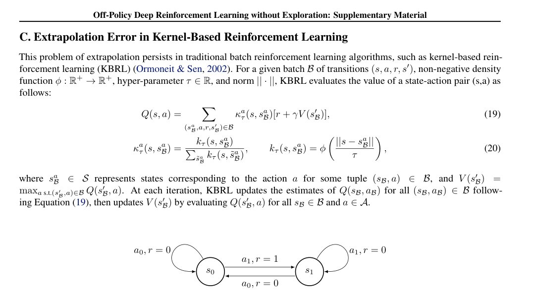
Figure 6: Toy MDP with two states and , and two actions and . Agent receives reward of for selecting at and otherwise.
图 6:两状态 、 与两动作 、 的玩具 MDP。智能体在 选 得奖励 ,其余为 。
Given access to the entire deterministic MDP, KBRL will provable converge to the optimal value, however when limited to only a subset, we find the value estimation susceptible to extrapolation. In Figure 6, we provide a deterministic two state, two action MDP in which KBRL fails to learn the optimal policy when provided with state-action pairs from the optimal policy. Given the batch , corresponding to the optimal behavior, and noting that there is only one example of each action, Equation (19) provides the following:
若能访问整个确定性 MDP,KBRL 可证明收敛到最优价值;但若仅限于子集,我们发现价值估计易受外推影响。图 6 给出一个确定性两状态、两动作 MDP:当只提供最优策略的状态–动作对时,KBRL 无法学到最优策略。给定对应最优行为的批次 ,并注意每个动作只有一个例子,公式 (19) 给出:
After sufficient iterations KBRL will converge correctly to , . However, when evaluating actions, KBRL erroneously extrapolates the values of each action , , and its behavior, , will result in the degenerate policy of continually selecting . KBRL fails this example by estimating the values of unseen state-action pairs. In methods where the extrapolated estimates can be included into the learning update, such fitted Q-iteration or DQN (Ernst et al. 2005; Mnih et al. 2015), this could cause an unbounded sequence of value estimates, as demonstrated by our results in Section 3.1.
足够迭代后 KBRL 会正确收敛到 、。但在评估动作时,KBRL 错误外推各动作价值 、,其行为 会得到持续选择 的退化策略。KBRL 因估计未见状态–动作对的价值而在此例失败。在外推估计可被纳入学习更新的方法中,如 fitted Q-iteration 或 DQN(Ernst et al. 2005;Mnih et al. 2015),这可能导致价值估计的无界序列,正如第 3.1 节结果所示。
Appendix D Additional Experiments
附录 D 额外实验
D.1 Ablation Study of Perturbation Model
D.1 扰动模型消融研究
BCQ includes a perturbation model which outputs a small residual update to the actions sampled by the generative model in the range . This enables the policy to select actions which may not have been sampled by the generative model. If , then all actions can be plausibly selected by the model, similar to standard deep reinforcement learning algorithms, such as DQN and DDPG (Mnih et al. 2015; Lillicrap et al. 2015). In Figure 7 we examine the performance and value estimates of BCQ when varying the hyper-parameter , which corresponds to how much the model is able to move away from the actions sampled by the generative model.
BCQ 包含扰动模型 ,在 范围内对生成模型采样的动作输出小的残差更新。这使策略能选择生成模型可能未采样到的动作。若 ,则模型可合理解释地选出全部动作,类似标准深度强化学习算法如 DQN 与 DDPG(Mnih et al. 2015;Lillicrap et al. 2015)。图 7 考察改变超参 (对应模型可离开生成模型采样动作多远)时 BCQ 的表现与价值估计。
(a)
We observe a clear drop in performance with the increase of , along with an increase in instability in the value function. Given that the data is based on expert performance, this is consistent with our understanding of extrapolation error. With larger the agent learns to take actions that are further away from the data in the batch after erroneously overestimating the value of suboptimal actions. This suggests the ideal value of should be small enough to stay close to the generated actions, but large enough such that learning can be performed when exploratory actions are included in the dataset.
我们观察到:随着 增大,表现明显下降,价值函数不稳定性增加。鉴于数据基于专家表现,这与我们对外推误差的理解一致。更大的 使智能体在错误高估次优动作后,学会采取离批次数据更远的动作。这表明 的理想值应足够小以贴近生成动作,又足够大以便数据集含探索动作时仍能学习。
D.2 Uncertainty Estimation for Batch-Constrained Reinforcement Learning
D.2 用于批次约束强化学习的不确定性估计
Section 4.2 proposes using generation as a method for constraining the output of the policy to eliminate actions which are unlikely under the batch. However, a more natural approach would be through approximate uncertainty-based methods (Osband et al. 2016; Gal et al. 2016; Azizzadenesheli et al. 2018). These methods are well-known to be effective for exploration, however we examine their properties for the exploitation where we would like to avoid uncertain actions.
第 4.2 节提出用生成作为约束策略 输出、以消除批次下不太可能动作的方法。但更自然的做法或许是近似基于不确定性的方法(Osband et al. 2016;Gal et al. 2016;Azizzadenesheli et al. 2018)。这些方法以探索闻名有效,我们则考察它们在利用中的性质——此时我们希望避开不确定动作。
To measure the uncertainty of the value network, we use ensemble-based methods, with an ensemble of size and to mimic the models used by Buckman et al. 2018 and Osband et al. 2016 respectively. Each network is trained with separate mini-batches, following the standard deep Q-learning update with a target network. These networks use the default architecture and hyper-parameter choices as defined in Section G. The policy is trained to minimize the standard deviation across the ensemble:
为度量价值网络的不确定性,我们使用基于集成的方法,集成大小分别为 与 ,以分别模仿 Buckman et al. 2018 与 Osband et al. 2016 所用模型。每个网络用独立小批次训练,遵循带目标网络的标准深度 Q 学习更新。这些网络使用第 G 节定义的默认架构与超参。策略 训练为最小化集成上的标准差 :
If the ensembles were a perfect estimate of the uncertainty, the policy would learn to select the most certain action for a given state, minimizing the extrapolation error and effectively imitating the data in the batch.
若集成是不确定性的完美估计,策略会学会对给定状态选最确定的动作,从而最小化外推误差并有效模仿批次数据。
To test these uncertainty-based methods, we examine their performance on the imitation task in the Hopper-v1 environment (Todorov et al. 2012; Brockman et al. 2016). In which a dataset of 1 million expert transitions are provided to the agents. Additional experimental details can be found in Section F. The performance, alongside the value estimates of the agents are displayed in Figure 8.
为测试这些基于不确定性的方法,我们在 Hopper-v1 环境(Todorov et al. 2012;Brockman et al. 2016)的 imitation 任务上考察其表现:向智能体提供 100 万次专家转移。更多实验细节见第 F 节。智能体表现与价值估计见图 8。
(a) Imitation performance
We find that neither ensemble method is sufficient to constrain the action space to only the expert actions. However, the value function is stabilized, suggesting that ensembles are an effective strategy for eliminating outliers or large deviations in the value from erroneous extrapolation. Unsurprisingly, the large ensemble provides a more accurate estimate of the uncertainty. While scaling the size of the ensemble to larger values could possibly enable an effective batch-constraint, increasing the size of the ensemble induces a large computational cost. Finally, in this task, where only expert data is provided, the policy can attempt to imitate the data without consideration of the value, however in other tasks, a weighting between value and uncertainty would need to be carefully tuned. On the other hand, BCQ offers a computational cheap approach without requirements for difficult hyper-parameter tuning.
我们发现两种集成方法都不足以把动作空间约束到仅专家动作。但价值函数得到稳定,说明集成是消除错误外推带来的离群或大幅价值偏离的有效策略。不出所料,更大集成对不确定性估计更准。把集成规模扩到更大或许能实现有效批次约束,但增大集成会带来高计算成本。最后,在只提供专家数据的该任务中,策略可试图模仿数据而不考虑价值;但在其他任务中,价值与不确定性之间的加权需要仔细调节。相比之下,BCQ 提供计算便宜、无需困难超参调节的方法。
D.3 Random Behavioral Policy Study
D.3 随机行为策略研究
The experiments in Section 3.1 and 5 use a learned, or partially learned, behavioral policy for data collection. This is a necessary requirement for learning meaningful behavior, as a random policy generally fails to provide sufficient coverage over the state space. However, in simple toy problems, such as the pendulum swing-up task and the reaching task with a two-joint arm from OpenAI gym (Brockman et al. 2016), a random policy can sufficiently explore the environment, enabling us to examine the properties of algorithms with entirely non-expert data.
第 3.1 节与第 5 节实验使用学到的或部分学到的行为策略采集数据。这对学到有意义行为是必要的,因为随机策略通常无法充分覆盖状态空间。但在简单玩具问题中,如 OpenAI gym(Brockman et al. 2016)的钟摆摆起任务与两关节臂到达任务,随机策略可充分探索环境,使我们能在完全非专家数据上考察算法性质。
In Figure 9, we examine the performance of our algorithm, BCQ, as well as DDPG (Lillicrap et al. 2015), on these two toy problems, when learning off-policy from a small batch of 5000 time steps, collected entirely by a random policy. We find that both BCQ and DDPG are able to learn successfully in these off-policy tasks. These results suggest that BCQ is less restrictive than imitation learning algorithms, which require expert data to learn. We also find that unlike previous environments, given the small scale of the state and action space, the random policy is able to provide sufficient coverage for DDPG to learn successfully.
图 9 考察我们的算法 BCQ 以及 DDPG(Lillicrap et al. 2015)在这两个玩具问题上的表现:从一个完全由随机策略采集的 5000 步小批次中离策略学习。我们发现 BCQ 与 DDPG 都能在这些离策略任务上成功学习。这些结果表明 BCQ 比需要专家数据才能学习的模仿学习算法限制更少。我们还发现:与先前环境不同,给定状态与动作空间的小规模,随机策略能为 DDPG 提供充分覆盖以成功学习。
(a) Random behavioral performance
Appendix E Missing Background
附录 E 缺失背景
E.1 Variational Auto-Encoder
E.1 变分自编码器
A variational auto-encoder (VAE) (Kingma & Welling 2013) is a generative model which aims to maximize the marginal log-likelihood where , the dataset. While computing the marginal likelihood is intractable in nature, we can instead optimize the variational lower-bound:
变分自编码器(VAE)(Kingma & Welling 2013)是旨在最大化边缘对数似然 的生成模型,其中 为数据集。尽管计算边缘似然本质上不可行,我们可改为优化变分下界:
where is chosen a prior, generally the multivariate normal distribution . We define the posterior as the encoder and as the decoder. Simply put, this means a VAE is an auto-encoder, where a given sample is passed through the encoder to produce a random latent vector , which is given to the decoder to reconstruct the original sample . The VAE is trained on a reconstruction loss, and a KL-divergence term according to the distribution of the latent vectors. To perform gradient descent on the variational lower bound we can use the re-parametrization trick (Kingma & Welling 2013; Rezende et al. 2014):
其中 取为先验,一般为多元正态 。我们将后验 定义为编码器, 为解码器。简单说,VAE 是自编码器:给定样本 经编码器产生随机潜向量 ,再交给解码器重建原样本 。VAE 按重建损失以及相对潜向量分布的 KL 散度项训练。要对变分下界做梯度下降,可用重参数化技巧(Kingma & Welling 2013;Rezende et al. 2014):
This formulation allows for back-propagation through stochastic nodes, by noting and can be represented by deterministic functions. During inference, random values of are sampled from the multivariate normal and passed through the decoder to produce samples .
该形式允许通过随机节点反向传播,因为 与 可由确定性函数表示。推断时从多元正态采样随机 ,经解码器产生样本 。
Appendix F Experimental Details
附录 F 实验细节
Each environment is run for 1 million time steps, unless stated otherwise, with evaluations every 5000 time steps, where an evaluation measures the average reward from 10 episodes with no exploration noise. Our results are reported over 5 random seeds of the behavioral policy, OpenAI Gym simulator and network initialization. Value estimates are averaged over mini-batches of and sampled every iterations. The true value is estimated by sampling state-action pairs from the buffer replay and computing the discounted return by running the episode until completion while following the current policy.
除非另有说明,每个环境运行 100 万时间步,每 5000 步评估一次;评估度量 10 个回合、无探索噪声的平均奖励。结果在行为策略、OpenAI Gym 模拟器与网络初始化的 5 个随机种子上报告。价值估计在大小为 的小批次上平均,每 次迭代采样一次。真实价值通过从回放缓冲采样 个状态–动作对,并按当前策略跑完回合计算折扣回报来估计。
Each agent is trained after each episode by applying one training iteration per each time step in the episode. The agent is trained with transition tuples sampled from an experience replay that is defined by each experiment. We define four possible experiments. Unless stated otherwise, default implementation settings, as defined in Section G, are used.
每个智能体在每回合结束后训练:对该回合每个时间步施加一次训练迭代。智能体用从各实验定义的经验回放中采样的转移元组 训练。我们定义四种可能实验。除非另有说明,使用第 G 节定义的默认实现设定。
Batch 1 (Final buffer). We train a DDPG (Lillicrap et al. 2015) agent for 1 million time steps, adding large amounts of Gaussian noise to induce exploration, and store all experienced transitions in a buffer replay. This training procedure creates a buffer replay with a diverse set of states and actions. A second, randomly initialized agent is trained using the 1 million stored transitions.
批次 1(最终缓冲)。 训练一个 DDPG(Lillicrap et al. 2015)智能体 100 万步,加入大量高斯噪声 以诱导探索,并将全部经历的转移存入回放缓冲。该训练过程产生状态与动作多样的回放缓冲。再用这 100 万条存储转移训练第二个随机初始化的智能体。
Batch 2 (Concurrent learning). We simultaneously train two agents for 1 million time steps, the first DDPG agent, performs data collection and each transition is stored in a buffer replay which both agents learn from. This means the behavioral agent learns from the standard training regime for most off-policy deep reinforcement learning algorithms, and the second agent is learning off-policy, as the data is collected without direct relationship to its current policy. Batch 2 differs from Batch 1 as the agents are trained with the same version of the buffer, while in Batch 1 the agent learns from the final buffer replay after the behavioral agent has finished training.
批次 2(并发学习)。 同时训练两个智能体共 100 万步:第一个 DDPG 智能体负责数据采集,每次转移存入两个智能体都从中学习的回放缓冲。这意味着行为智能体按多数离策略深度强化学习算法的标准训练体制学习,第二个智能体则在离策略学习,因为数据的采集与其当前策略无直接关系。批次 2 与批次 1 的不同在于:智能体用同一版本缓冲训练;而批次 1 中智能体在行为智能体训练结束后,从最终回放缓冲学习。
Batch 3 (Imitation). A DDPG agent is trained for 1 million time steps. The trained agent then acts as an expert policy, and is used to collect a dataset of 1 million transitions. This dataset is used to train a second, randomly initialized agent. In particular, we train DDPG across 15 seeds, and select the 5 top performing seeds as the expert policies.
批次 3(模仿)。 训练一个 DDPG 智能体 100 万步。训练好的智能体充当专家策略,用于采集 100 万次转移的数据集。该数据集用于训练第二个随机初始化的智能体。具体地,我们在 15 个种子上训练 DDPG,并选取表现最好的 5 个种子作为专家策略。
Batch 4 (Imperfect demonstrations). The expert policies from Batch 3 are used to collect a dataset of 100k transitions, while selecting actions randomly with probability and adding Gaussian noise to the remaining actions. This dataset is used to train a second, randomly initialized agent.
批次 4(不完美示范)。 用批次 3 的专家策略采集 10 万次转移的数据集,同时以概率 随机选动作,并对其余动作加高斯噪声 。该数据集用于训练第二个随机初始化的智能体。
Appendix G Implementation Details
附录 G 实现细节
Across all methods and experiments, for fair comparison, each network generally uses the same hyper-parameters and architecture, which are defined in Table 1 and Figure 10 respectively. The value functions follow the standard practice (Mnih et al. 2015) in which the Bellman update differs for terminal transitions. When the episode ends by reaching some terminal state, the value is set to in the learning target :
为公平对比,所有方法与实验中,每个网络一般使用相同超参与架构,分别见表 1 与图 10。价值函数遵循标准做法(Mnih et al. 2015):对终止转移,Bellman 更新不同。当回合因到达某终止状态而结束时,学习目标 中价值设为 :
$$y=\begin{cases}r&\text{if terminal }s^{\prime}\
r+\gamma Q_{\theta^{\prime}}(s^{\prime},a^{\prime})&\text{else}\
\end{cases} \tag{25}$$
Where the termination signal from time-limited environments is ignored, thus we only consider a state terminal if max horizon.
其中忽略来自有时限环境的终止信号,因而仅当 最大时域时才将状态 视为终止。
| Hyper-parameter | Value |
|---|---|
| Optimizer | Adam (Kingma & Ba 2014) |
| Learning Rate | |
| Batch Size | |
| Normalized Observations | False |
| Gradient Clipping | False |
| Discount Factor | |
| Target Update Rate () | |
| Exploration Policy |
Table 1: Default hyper-parameters.
| Hyper-parameter | Value |
|---|---|
| Optimizer | Adam (Kingma & Ba 2014) |
| Learning Rate | |
| Batch Size | |
| Normalized Observations | False |
| Gradient Clipping | False |
| Discount Factor | |
| Target Update Rate () | |
| Exploration Policy |
表 1:默认超参。
(input dimension, 400) ReLU (400, 300) RelU (300, output dimension)
(input dimension, 400)
ReLU
(400, 300)
RelU
(300, output dimension)
Figure 10: Default network architecture, based on DDPG (Lillicrap et al. 2015). All actor networks are followed by a tanh max action size
(input dimension, 400) ReLU (400, 300) RelU (300, output dimension)
(input dimension, 400)
ReLU
(400, 300)
RelU
(300, output dimension)
图 10:默认网络架构,基于 DDPG(Lillicrap et al. 2015)。所有 actor 网络后接 tanh · 最大动作幅度
BCQ. BCQ uses four main networks: a perturbation model , a state-conditioned VAE and a pair of value networks . Along with three corresponding target networks . Each network, other than the VAE follows the default architecture (Figure 10) and the default hyper-parameters (Table 1). For , the constraint is implemented through a tanh activation multiplied by following the final layer.
BCQ。 BCQ 使用四个主网络:扰动模型 、状态条件 VAE ,以及一对价值网络 。另有三个对应目标网络 。除 VAE 外,每个网络遵循默认架构(图 10)与默认超参(表 1)。对 ,约束 通过末层后的 tanh 激活再乘以 实现。
As suggested by Fujimoto et al. 2018, the perturbation model is trained only with respect to , following the deterministic policy gradient algorithm (Silver et al. 2014), by performing a residual update on a single action sampled from the generative model:
如 Fujimoto et al. 2018 所建议,扰动模型只相对 训练,遵循确定性策略梯度算法(Silver et al. 2014),对从生成模型采样的单个动作做残差更新:
$$\begin{split}\phi&\leftarrow\argmax_{\phi}\sum_{(s,a)\in\mathcal{B}}Q_{\theta_{1}}(s,a+\xi_{\phi}(s,a,\Phi)),\
&a\sim G_{\omega}(s).\end{split} \tag{26}$$
To penalize uncertainty over future states, we train a pair of value estimates and take a weighted minimum between the two values as a learning target for both networks. First actions are sampled with respect to the generative model, and then adjusted by the target perturbation model, before passed to each target Q-network:
为惩罚对未来状态的不确定性,我们训练一对价值估计 ,并取两价值的加权最小值作为两个网络共用的学习目标 。先按生成模型采样 个动作,再由目标扰动模型调整,然后送入各目标 Q 网络:
$$\begin{split}y&=r+\gamma\max_{ai}\left[\lambda\min_{j=1,2}Q_{\theta^{\prime}{j}}(s^{\prime},\tilde{a}{i})+(1-\lambda)\max_{j=1,2}Q_{\theta^{\prime}{j}}(s^{\prime},\tilde{a}{i})\right],\
&{\tilde{a}{i}=a{i}+\xi_{\phi^{\prime}}(s,a_{i},\Phi)}{i=0}^{n},\qquad{a{i}\sim G_{\omega}(s^{\prime})}{i=0}^{n},\
&\mathcal{L}{\text{value,i}}=\sum_{(s,a,r,s^{\prime})\in\mathcal{B}}(y-Q_{\theta_{i}}(s,a))^{2}.\end{split} \tag{27}$$
Both networks are trained with the same target , where .
两个网络用同一目标 训练,其中 。
The VAE is defined by two networks, an encoder and decoder , where . The encoder takes a state-action pair and outputs the mean and standard deviation of a Gaussian distribution . The state , along with a latent vector is sampled from the Gaussian, is passed to the decoder which outputs an action. Each network follows the default architecture (Figure 10), with two hidden layers of size , rather than and . The VAE is trained with respect to the mean squared error of the reconstruction along with a KL regularization term:
VAE 由两个网络定义:编码器 与解码器 ,其中 。编码器接受状态–动作对,输出高斯分布 的均值 与标准差 。状态 与从该高斯采样的潜向量 一起送入解码器 ,输出一个动作。每个网络遵循默认架构(图 10),但两层隐层大小为 ,而非 与 。VAE 按重建均方误差以及 KL 正则项训练:
Noting the Gaussian form of both distributions, the KL divergence term can be simplified (Kingma & Welling 2013):
注意两种分布的高斯形式,KL 散度项可化简(Kingma & Welling 2013):
where denotes the dimensionality of . For each experiment, is set to twice the dimensionality of the action space. The KL divergence term in is normalized across experiments by setting . During inference with the VAE, the latent vector is clipped to a range of to limit generalization beyond previously seen actions. For the small scale experiments in Supplementary Material D.3, regularization with weight was used for the VAE to compensate for the small number of samples. The other networks remain unchanged. In the value network update (Equation 27), the VAE is sampled multiple times and passed to both the perturbation model and each Q-network. For each state in the mini-batch the VAE is sampled times. This can be implemented efficiently by passing a latent vector with batch size batch size, effectively , to the VAE and treating the output as a new mini-batch for the perturbation model and each Q-network. When running the agent in the environment, we sample from the VAE times, perturb each action with and sample the highest valued action with respect to .
其中 表示 的维数。每个实验中 取为动作空间维数的两倍。通过设 , 中的 KL 散度项在各实验间归一化。用 VAE 推断时,潜向量 被裁剪到 ,以限制超出先前所见动作的泛化。对补充材料 D.3 的小规模实验,VAE 使用权重 的 正则以补偿样本数少。其他网络保持不变。在价值网络更新(公式 27)中,VAE 被多次采样并送入扰动模型与各 Q 网络。对小批次中每个状态,VAE 采样 次。这可通过向 VAE 传入批次大小为 · 批次大小(即有效为 )的潜向量,并把输出当作扰动模型与各 Q 网络的新小批次来高效实现。在环境中运行智能体时,我们从 VAE 采样 10 次,用 扰动每个动作,并相对 采样最高价值动作。
DDPG. Our DDPG implementation deviates from some of the default architecture and hyper-parameters to mimic the original implementation more closely (Lillicrap et al. 2015). In particular, the action is only passed to the critic at the second layer (Figure 11), the critic uses regularization with weight , and the actor uses a reduced learning rate of .
DDPG。 我们的 DDPG 实现偏离部分默认架构与超参,以更贴近原实现(Lillicrap et al. 2015)。具体地,动作仅在第二层传入 critic(图 11),critic 使用权重 的 正则,actor 使用降低后的学习率 。
(state dimension, 400) ReLU (400 + action dimension, 300) RelU (300, 1)
(state dimension, 400)
ReLU
(400 + action dimension, 300)
RelU
(300, 1)
Figure 11: DDPG Critic Network Architecture.
(state dimension, 400) ReLU (400 + action dimension, 300) RelU (300, 1)
(state dimension, 400)
ReLU
(400 + action dimension, 300)
RelU
(300, 1)
图 11:DDPG Critic 网络架构。
As done by Fujimoto et al. 2018, our DDPG agent randomly selects actions for the first 10k time steps for HalfCheetah-v1, and 1k time steps for Hopper-v1 and Walker2d-v1. This was found to improve performance and reduce the likelihood of local minima in the policy during early iterations.
如 Fujimoto et al. 2018 所做,我们的 DDPG 智能体在 HalfCheetah-v1 前 10k 步、Hopper-v1 与 Walker2d-v1 前 1k 步随机选动作。这被发现可改善表现并降低早期迭代中策略落入局部极小的可能性。
DQN. Given the high dimensional nature of the action space of the experimental environments, our DQN implementation selects actions over an independently discretized action space. Each action dimension is discretized separately into possible actions, giving possible actions, where is the dimensionality of the action-space. A given state-action pair then corresponds to a set of state-sub-action pairs , where bins and dimensions. In each DQN update, all state-sub-action pairs are updated with respect to the average value of the target state-sub-action pairs . The learning update of the discretized DQN is as follows:
DQN。 鉴于实验环境动作空间的高维性质,我们的 DQN 实现在独立离散化的动作空间上选动作。每个动作维单独离散为 个可能动作,共 个可能动作,其中 为动作空间维数。给定状态–动作对 对应一组状态–子动作对 ,其中 为分箱, 为维。每次 DQN 更新中,所有状态–子动作对 相对目标状态–子动作对 的平均价值更新。离散化 DQN 的学习更新如下:
Where is chosen by selecting the corresponding bin in the discretized action space for each dimension . For clarity, we provide the exact DQN network architecture in Figure 12.
其中 通过对每个维 在离散动作空间中选择对应分箱 得到。为清晰起见,我们在图 12 给出精确的 DQN 网络架构。
(state dimension, 400) ReLU (400, 300) RelU (300, 10 action dimension)
(state dimension, 400)
ReLU
(400, 300)
RelU
(300, 10 action dimension)
Figure 12: DQN Network Architecture.
(state dimension, 400) ReLU (400, 300) RelU (300, 10 action dimension)
(state dimension, 400)
ReLU
(400, 300)
RelU
(300, 10 action dimension)
图 12:DQN 网络架构。
Behavioral Cloning. We use two behavioral cloning methods, VAE-BC and BC. VAE-BC is implemented and trained exactly as defined for BCQ. BC uses a feed-forward network with the default architecture and hyper-parameters, and trained with a mean-squared error reconstruction loss.
行为克隆。 我们使用两种行为克隆方法:VAE-BC 与 BC。VAE-BC 的实现与训练完全同 BCQ 中定义的 。BC 使用默认架构与超参的前馈网络,并以均方误差重建损失训练。