Barlow Twins: Self-Supervised Learning via Redundancy Reduction
Barlow Twins: Self-Supervised Learning via Redundancy Reduction
Abstract
摘要
Self-supervised learning (SSL) is rapidly closing the gap with supervised methods on large computer vision benchmarks. A successful approach to SSL is to learn embeddings which are invariant to distortions of the input sample. However, a recurring issue with this approach is the existence of trivial constant solutions. Most current methods avoid such solutions by careful implementation details. We propose an objective function that naturally avoids collapse by measuring the cross-correlation matrix between the outputs of two identical networks fed with distorted versions of a sample, and making it as close to the identity matrix as possible. This causes the embedding vectors of distorted versions of a sample to be similar, while minimizing the redundancy between the components of these vectors. The method is called BARLOW TWINS, owing to neuroscientist H. Barlow's redundancy-reduction principle applied to a pair of identical networks. BARLOW TWINS does not require large batches nor asymmetry between the network twins such as a predictor network, gradient stopping, or a moving average on the weight updates. Intriguingly it benefits from very high-dimensional output vectors. BARLOW TWINS outperforms previous methods on ImageNet for semi-supervised classification in the low-data regime, and is on par with current state of the art for ImageNet classification with a linear classifier head, and for transfer tasks of classification and object detection.
自监督学习(SSL)在大型计算机视觉基准上,正迅速缩小与有监督方法的差距。一类成功的做法,是学习对输入样本的扰动保持不变的嵌入。不过,这条路线反复遇到一个问题:存在平凡的常数解。现有方法大多靠仔细设计的实现细节来避开这类解。我们提出一种目标函数,通过度量两个相同网络在同一样本的扰动版本上的输出互相关矩阵、并使其尽可能接近单位矩阵,从而自然避免坍缩。这样做会让同一样本不同扰动版本的嵌入向量彼此相似,同时尽量降低这些向量各分量之间的冗余。该方法称作 BARLOW TWINS,得名于神经科学家 H. Barlow 的冗余减少原则,并把它用到一对相同网络上。BARLOW TWINS 不需要大批次,也不需要孪生网络之间的不对称,例如预测网络、停止梯度,或权重更新上的滑动平均。一个有意思的现象是,它还能从非常高维的输出向量中受益。在 ImageNet 的低数据半监督分类上,BARLOW TWINS 优于已有方法;在带线性分类头的 ImageNet 分类,以及分类和目标检测等迁移任务上,它与当时的最先进结果相当。
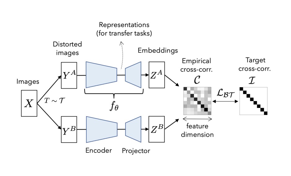
Figure 1. BARLOW TWINS's objective function measures the cross-correlation matrix between the embeddings of two identical networks fed with distorted versions of a batch of samples, and tries to make this matrix close to the identity. This causes the embedding vectors of distorted versions of a sample to be similar, while minimizing the redundancy between the components of these vectors. BARLOW TWINS is competitive with state-of-the-art methods for self-supervised learning while being conceptually simpler, naturally avoiding trivial constant (i.e. collapsed) embeddings, and being robust to the training batch size.
图 1:BARLOW TWINS 的目标函数度量两个相同网络的嵌入之间的互相关矩阵,这两个网络分别接收一个批次样本的扰动版本,并试图让该矩阵接近单位矩阵。这样做会让同一样本不同扰动版本的嵌入向量彼此相似,同时尽量降低这些向量各分量之间的冗余。BARLOW TWINS 在概念上更简单,能自然避免平凡的常数(即坍缩)嵌入,并且对训练批次大小稳健,同时与自监督学习的最先进方法具有竞争力。
- Introduction
- 引言
Self-supervised learning aims to learn useful representations of the input data without relying on human annotations. Recent advances in self-supervised learning for visual data (Caron et al., 2020; Chen et al., 2020a; Grill et al., 2020; He et al., 2019; Misra & van der Maaten, 2019) show that it is possible to learn self-supervised representations that are competitive with supervised representations. A common underlying theme that unites these methods is that they all aim to learn representations that are invariant under different distortions (also referred to as 'data augmentations'). This is typically achieved by maximizing similarity of representations obtained from different distorted versions of a sample using a variant of Siamese networks (Hadsell et al., 2006). As there are trivial solutions to this problem, like a constant representation, these methods rely on different mechanisms to learn useful representations.
自监督学习的目标,是在不依赖人工标注的情况下,学习对输入数据有用的表征。视觉数据自监督学习的近期进展(Caron et al., 2020; Chen et al., 2020a; Grill et al., 2020; He et al., 2019; Misra & van der Maaten, 2019)表明,有可能学到与有监督表征相竞争的自监督表征。这些方法有一个共同主题:都力求学习在不同扰动(也称作“数据增强”)下保持不变的表征。实现方式通常是,用某种孪生网络变体(Hadsell et al., 2006),最大化同一样本不同扰动版本所得表征之间的相似性。由于这个问题存在平凡解,例如常数表征,这些方法要依靠不同机制才能学到有用的表征。
Contrastive methods like SIMCLR (Chen et al., 2020a) define 'positive' and 'negative' sample pairs which are treated differently in the loss function. Additionally, they can also use asymmetric learning updates wherein momentum encoders (He et al., 2019) are updated separately from the main network. Clustering methods use one distorted sample to compute 'targets' for the loss, and another distorted version of the sample to predict these targets, followed by an alternate optimization scheme like k-means in DEEPCLUSTER (Caron et al., 2018) or non-differentiable operators in SWAV (Caron et al., 2020) and SELA (Asano et al., 2020). In another recent line of work, BYOL (Grill et al., 2020) and SIMSIAM (Chen & He, 2020), both the network architecture and parameter updates are modified to introduce asymmetry. The network architecture is modified to be asymmetric using a special 'predictor' network and the parameter updates are asymmetric such that the model parameters are only updated using one distorted version of the input, while the representations from another distorted version are used as a fixed target. (Chen & He, 2020) conclude that the asymmetry of the learning update, 'stop-gradient', is critical to preventing trivial solutions.
像 SIMCLR(Chen et al., 2020a)这样的对比方法会定义“正”样本对和“负”样本对,并在损失函数中区别对待。此外,它们也可以采用不对称的学习更新,让动量编码器(He et al., 2019)与主网络分开更新。聚类方法用一个扰动样本计算损失的“目标”,再用该样本的另一个扰动版本去预测这些目标,随后进行交替优化,例如 DEEPCLUSTER 中的 k-means(Caron et al., 2018),或 SWAV(Caron et al., 2020)和 SELA(Asano et al., 2020)中的不可微算子。在另一类近期工作中,BYOL(Grill et al., 2020)和 SIMSIAM(Chen & He, 2020)同时修改网络结构和参数更新,以引入不对称。网络结构通过一个专门的“预测”网络变得不对称;参数更新也不对称:模型参数只根据输入的一个扰动版本来更新,另一个扰动版本的表征则用作固定目标。(Chen & He, 2020)的结论是,学习更新上的不对称,即“停止梯度”(stop-gradient),对防止平凡解至关重要。
In this paper, we propose a new method, BARLOW TWINS, which applies redundancy-reduction — a principle first proposed in neuroscience — to self-supervised learning. In his influential article Possible Principles Underlying the Transformation of Sensory Messages (Barlow, 1961), neuroscientist H. Barlow hypothesized that the goal of sensory processing is to recode highly redundant sensory inputs into a factorial code (a code with statistically independent components). This principle has been fruitful in explaining the organization of the visual system, from the retina to cortical areas (see (Barlow, 2001) for a review and (Lindsey et al., 2020; Ocko et al., 2018; Schwartz & Simoncelli, 2001) for recent efforts), and has led to a number of algorithms for supervised and unsupervised learning (Ballé et al., 2017; Deco & Parra, 1997; Földiák, 1990; Linsker, 1988; Redlich, 1993a;b; Schmidhuber et al., 1996). Based on this principle, we propose an objective function which tries to make the cross-correlation matrix computed from twin embeddings as close to the identity matrix as possible. BARLOW TWINS is conceptually simple, easy to implement and learns useful representations as opposed to trivial solutions. Compared to other methods, it does not require large batches (Chen et al., 2020a), nor does it require any asymmetric mechanisms like prediction networks (Grill et al., 2020), momentum encoders (He et al., 2019), non-differentiable operators (Caron et al., 2020) or stop-gradients (Chen & He, 2020). Intriguingly, BARLOW TWINS strongly benefits from the use of very high-dimensional embeddings. BARLOW TWINS outperforms previous methods on ImageNet for semi-supervised classification in the low-data regime (55% top-1 accuracy for 1% labels), and is on par with current state of the art for ImageNet classification with a linear classifier head, as well as for a number of transfer tasks of classification and object detection.
本文提出一种新方法 BARLOW TWINS,把冗余减少——这一首先在神经科学中提出的原则——用于自监督学习。在那篇有影响的文章 Possible Principles Underlying the Transformation of Sensory Messages(Barlow, 1961)中,神经科学家 H. Barlow 提出:感官加工的目标,是把高度冗余的感官输入重新编码成因子码(各分量统计独立的编码)。这一原则在解释视觉系统从视网膜到皮层的组织方式上颇有成效(综述见 (Barlow, 2001),近期工作见 (Lindsey et al., 2020; Ocko et al., 2018; Schwartz & Simoncelli, 2001)),并引出一批有监督与无监督学习算法(Ballé et al., 2017; Deco & Parra, 1997; Földiák, 1990; Linsker, 1988; Redlich, 1993a;b; Schmidhuber et al., 1996)。基于这一原则,我们提出一种目标函数,试图让由孪生嵌入算得的互相关矩阵尽可能接近单位矩阵。BARLOW TWINS 在概念上简单、易于实现,并且学到的是有用表征而非平凡解。与其他方法相比,它不需要大批次(Chen et al., 2020a),也不需要预测网络(Grill et al., 2020)、动量编码器(He et al., 2019)、不可微算子(Caron et al., 2020)或停止梯度(Chen & He, 2020)这类不对称机制。一个有意思的现象是,BARLOW TWINS 能从非常高维的嵌入中显著受益。在 ImageNet 的低数据半监督分类上,BARLOW TWINS 优于已有方法(1% 标注时 Top-1 准确率为 55%);在带线性分类头的 ImageNet 分类,以及若干分类和目标检测迁移任务上,它与当时的最先进结果相当。
*Equal contribution 1Facebook AI Research 2New York University, NY, USA. Correspondence to: Jure Zbontar jzb@fb.com, Li Jing ljng@fb.com, Ishan Misra imisra@fb.com, Yann LeCun yann@fb.com, Stéphane Deny stephane.deny.pro@gmail.com.
Proceedings of the 38 International Conference on Machine Learning, PMLR 139, 2021. Copyright 2021 by the author(s).
Code and pre-trained models (in PyTorch) are available at https://github.com/facebookresearch/barlowtwins
代码与预训练模型(PyTorch)见 https://github.com/facebookresearch/barlowtwins
- Method
- 方法
2.1. Description of BARLOW TWINS
2.1. BARLOW TWINS 的描述
Like other methods for SSL (Caron et al., 2020; Chen et al., 2020a; Grill et al., 2020; He et al., 2019; Misra & van der Maaten, 2019), BARLOW TWINS operates on a joint embedding of distorted images (Fig. 1). More specifically, it produces two distorted views for all images of a batch sampled from a dataset. The distorted views are obtained via a distribution of data augmentations . The two batches of distorted views and are then fed to a function , typically a deep network with trainable parameters , producing batches of embeddings and respectively. To simplify notations, and are assumed to be mean-centered along the batch dimension, such that each unit has mean output 0 over the batch.
与其他自监督学习方法一样(Caron et al., 2020; Chen et al., 2020a; Grill et al., 2020; He et al., 2019; Misra & van der Maaten, 2019),BARLOW TWINS 作用于扰动图像的联合嵌入(图 1)。更具体地说,它对从数据集中采样的一个批次 中的所有图像,各产生两个扰动视图。这些扰动视图由数据增强分布 得到。随后,两个扰动视图批次 和 被送入函数 (通常是带可训练参数 的深度网络),分别得到嵌入批次 和 。为简化记号,假定 和 已沿批次维做了均值中心化,从而使每个单元在批次上的平均输出为 0。
BARLOW TWINS distinguishes itself from other methods by its innovative loss function :
BARLOW TWINS 与其他方法的不同之处,在于它创新的损失函数 :
where is a positive constant trading off the importance of the first and second terms of the loss, and where is the cross-correlation matrix computed between the outputs of the two identical networks along the batch dimension:
其中 是权衡损失第一项与第二项重要性的正常数, 是沿批次维、在两个相同网络的输出之间计算的互相关矩阵:
where indexes batch samples and index the vector dimension of the networks' outputs. is a square matrix with size the dimensionality of the network's output, and with values comprised between -1 (i.e. perfect anti-correlation) and 1 (i.e. perfect correlation).
其中 标示批次中的样本,、 标示网络输出的向量维度。 是方阵,边长等于网络输出的维度,取值介于 -1(即完全反相关)和 1(即完全相关)之间。
Intuitively, the invariance term of the objective, by trying to equate the diagonal elements of the cross-correlation matrix to 1, makes the embedding invariant to the distortions applied. The redundancy reduction term, by trying to equate the off-diagonal elements of the cross-correlation matrix to 0, decorrelates the different vector components of the embedding. This decorrelation reduces the redundancy between output units, so that the output units contain non-redundant information about the sample.
直观上,目标中的不变性项试图让互相关矩阵的对角元等于 1,从而使嵌入对所施加的扰动保持不变。冗余减少项则试图让互相关矩阵的非对角元等于 0,从而解除嵌入中不同向量分量之间的相关。这种去相关降低了输出单元之间的冗余,使各输出单元包含关于该样本的非冗余信息。
More formally, BARLOW TWINS's objective function can be understood through the lens of information theory, and specifically as an instanciation of the Information Bottleneck (IB) objective (Tishby & Zaslavsky, 2015; Tishby et al., 2000). Applied to self-supervised learning, the IB objective consists in finding a representation that conserves as much information about the sample as possible while being the least possible informative about the specific distortions applied to that sample. The mathematical connection between BARLOW TWINS's objective function and the IB principle is explored in Appendix A.
更形式地说,BARLOW TWINS 的目标函数可以从信息论的角度来理解,具体而言,它是信息瓶颈(Information Bottleneck, IB)目标的一个实例(Tishby & Zaslavsky, 2015; Tishby et al., 2000)。用于自监督学习时,IB 目标是要找到这样一种表征:尽可能多地保留关于样本的信息,同时尽可能少地包含关于施加在该样本上的特定扰动的信息。BARLOW TWINS 的目标函数与 IB 原则之间的数学联系,在附录 A 中讨论。
BARLOW TWINS' objective function has similarities with existing objective functions for SSL. For example, the redundancy reduction term plays a role similar to the contrastive term in the INFONCE objective (Oord et al., 2018), as discussed in detail in Section 5. However, important conceptual differences in these objective functions result in practical advantages of our method compared to INFONCE-based methods, namely that (1) our method does not require a large number of negative samples and can thus operate on small batches (2) our method benefits from very high-dimensional embeddings. Alternatively, the redundancy reduction term can be viewed as a soft-whitening constraint on the embeddings, connecting our method to a recently proposed method performing a hard-whitening operation on the embeddings (Ermolov et al., 2020), as discussed in Section 5. However, our method performs better than current hard-whitening methods.
BARLOW TWINS 的目标函数与已有的自监督学习目标有相似之处。例如,冗余减少项所起的作用,类似于 INFONCE 目标中的对比项(Oord et al., 2018),第 5 节会详细讨论。不过,这些目标函数在概念上的重要差异,也带来了我们的方法相对于基于 INFONCE 的方法的实际优点,即:(1) 我们的方法不需要大量负样本,因而可以在小批次上运行;(2) 我们的方法能从非常高维的嵌入中受益。另外,冗余减少项也可以看成对嵌入的一种软白化约束,从而把我们的方法与最近提出的、对嵌入做硬白化操作的方法(Ermolov et al., 2020)联系起来,见第 5 节。不过,我们的方法优于目前的硬白化方法。
The pseudocode for BARLOW TWINS is shown as Algorithm 1.
BARLOW TWINS 的伪代码见算法 1。
Algorithm 1 PyTorch-style pseudocode for Barlow Twins.
# f: encoder network
# lambda: weight on the off-diagonal terms
# N: batch size
# D: dimensionality of the embeddings
#
# mm: matrix-matrix multiplication
# off_diagonal: off-diagonal elements of a matrix
# eye: identity matrix

for x in loader: # load a batch with N samples
    # two randomly augmented versions of x
    y_a, y_b = augment(x)

    # compute embeddings
    z_a = f(y_a) # NxD
    z_b = f(y_b) # NxD

    # normalize repr. along the batch dimension
    z_a_norm = (z_a - z_a.mean(0)) / z_a.std(0) # NxD
    z_b_norm = (z_b - z_b.mean(0)) / z_b.std(0) # NxD

    # cross-correlation matrix
    c = mm(z_a_norm.T, z_b_norm) / N # DxD

    # loss
    c_diff = (c - eye(D)).pow(2) # DxD
    # multiply off-diagonal elems of c_diff by lambda
    off_diagonal(c_diff).mul_(lambda)
    loss = c_diff.sum()

    # optimization step
    loss.backward()
    optimizer.step()
算法 1 Barlow Twins 的 PyTorch 风格伪代码。
# f: 编码器网络
# lambda: 非对角项的权重
# N: 批次大小
# D: 嵌入的维度
#
# mm: 矩阵-矩阵乘法
# off_diagonal: 矩阵的非对角元
# eye: 单位矩阵

for x in loader: # 载入一个含 N 个样本的批次
    # x 的两个随机增强版本
    y_a, y_b = augment(x)

    # 计算嵌入
    z_a = f(y_a) # NxD
    z_b = f(y_b) # NxD

    # 沿批次维归一化表征
    z_a_norm = (z_a - z_a.mean(0)) / z_a.std(0) # NxD
    z_b_norm = (z_b - z_b.mean(0)) / z_b.std(0) # NxD

    # 互相关矩阵
    c = mm(z_a_norm.T, z_b_norm) / N # DxD

    # 损失
    c_diff = (c - eye(D)).pow(2) # DxD
    # 将 c_diff 的非对角元乘以 lambda
    off_diagonal(c_diff).mul_(lambda)
    loss = c_diff.sum()

    # 优化步骤
    loss.backward()
    optimizer.step()
2.2. Implementation Details
2.2. 实现细节
Image augmentations Each input image is transformed twice to produce the two distorted views shown in Figure 1. The image augmentation pipeline consists of the following transformations: random cropping, resizing to , horizontal flipping, color jittering, converting to grayscale, Gaussian blurring, and solarization. The first two transformations (cropping and resizing) are always applied, while the last five are applied randomly, with some probability. This probability is different for the two distorted views in the last two transformations (blurring and solarization). We use the same augmentation parameters as BYOL (Grill et al., 2020).
图像增强。每张输入图像会被变换两次,以产生图 1 中所示的两个扰动视图。图像增强流水线包含以下变换:随机裁剪、缩放到 、水平翻转、颜色抖动、转为灰度、高斯模糊,以及日晒化(solarization)。前两个变换(裁剪和缩放)总会施加,后五个则以一定概率随机施加。对最后两个变换(模糊和日晒化),两个扰动视图所用的概率不同。我们使用与 BYOL(Grill et al., 2020)相同的增强参数。
Architecture The encoder consists of a ResNet-50 network (He et al., 2016) (without the final classification layer, 2048 output units) followed by a projector network. The projector network has three linear layers, each with 8192 output units. The first two layers of the projector are followed by a batch normalization layer and rectified linear units. We call the output of the encoder the 'representations' and the output of the projector the 'embeddings'. The representations are used for downstream tasks and the embeddings are fed to the loss function of BARLOW TWINS.
架构。编码器由一个 ResNet-50 网络(He et al., 2016)(去掉最后的分类层,输出 2048 个单元)后接一个投影网络组成。投影网络有三个线性层,每层 8192 个输出单元。投影网络的前两层之后接批归一化层和修正线性单元。我们把编码器的输出称作“表征”,把投影网络的输出称作“嵌入”。表征用于下游任务,嵌入则送入 BARLOW TWINS 的损失函数。
Optimization We follow the optimization protocol described in BYOL (Grill et al., 2020). We use the LARS optimizer (You et al., 2017) and train for 1000 epochs with a batch size of 2048. We however emphasize that our model works well with batches as small as 256 (see Ablations). We use a learning rate of 0.2 for the weights and 0.0048 for the biases and batch normalization parameters. We multiply the learning rate by the batch size and divide it by 256. We use a learning rate warm-up period of 10 epochs, after which we reduce the learning rate by a factor of 1000 using a cosine decay schedule (Loshchilov & Hutter, 2016). We ran a search for the trade-off parameter of the loss function and found the best results for . We use a weight decay parameter of . The biases and batch normalization parameters are excluded from LARS adaptation and weight decay. Training is distributed across 32 V100 GPUs and takes approximately 124 hours. For comparison, our reimplementation of BYOL trained with a batch size of 4096 takes 113 hours on the same hardware.
优化。我们沿用 BYOL(Grill et al., 2020)中描述的优化协议。我们使用 LARS 优化器(You et al., 2017),训练 1000 个周期,批次大小为 2048。不过我们要强调,模型在批次小到 256 时仍然表现良好(见消融实验)。权重的学习率为 0.2,偏置和批归一化参数的学习率为 0.0048。我们把学习率乘以批次大小再除以 256。学习率有 10 个周期的预热,之后用余弦衰减计划(Loshchilov & Hutter, 2016)把学习率缩小 1000 倍。我们搜索了损失函数的权衡参数 ,在 时得到最好结果。权重衰减参数取 。偏置和批归一化参数不参与 LARS 自适应和权重衰减。训练分布在 32 块 V100 GPU 上,大约需要 124 小时。作为比较,我们重实现的 BYOL 在批次大小 4096、同一硬件上训练需要 113 小时。
- Results
- 结果
We follow standard practice (Goyal et al., 2019) and evaluate our representations by transfer learning to different datasets and tasks in computer vision. Our network is pre-trained using self-supervised learning on the training set of the ImageNet ILSVRC-2012 dataset (Deng et al., 2009) (without labels). We evaluate our model on a variety of tasks such as image classification and object detection, and using fixed representations from the network or finetuning it. We provide the hyperparameters for all the transfer learning experiments in the Appendix.
我们沿用通行做法(Goyal et al., 2019),通过把表征迁移到计算机视觉中不同的数据集和任务上来评估。网络在 ImageNet ILSVRC-2012 数据集(Deng et al., 2009)的训练集上用自监督学习预训练(不使用标签)。我们在图像分类、目标检测等多种任务上评估模型,既使用网络的固定表征,也对网络做微调。各迁移学习实验的超参数见附录。
3.1. Linear and Semi-Supervised Evaluations on ImageNet
3.1. 在 ImageNet 上的线性评估与半监督评估
Linear evaluation on ImageNet We train a linear classifier on ImageNet on top of fixed representations of a ResNet-50 pretrained with our method. The top-1 and top-5 accuracies obtained on the ImageNet validation set are reported in Table 1. Our method obtains a top-1 accuracy of 73.2% which is comparable to the state-of-the-art methods.
ImageNet 上的线性评估。我们在用本方法预训练的 ResNet-50 的固定表征之上,于 ImageNet 上训练一个线性分类器。在 ImageNet 验证集上得到的 Top-1 和 Top-5 准确率见表 1。我们的方法取得 73.2% 的 Top-1 准确率,与最先进的方法相当。
Table 1. Top-1 and top-5 accuracies (in %) under linear evaluation on ImageNet. All models use a ResNet-50 encoder. Top-3 best self-supervised methods are underlined.
| Method | Top-1 | Top-5 |
|---|---|---|
| Supervised | 76.5 | |
| MoCo | 60.6 | |
| PIRL | 63.6 | - |
| SIMCLR | 69.3 | 89.0 |
| MoCo v2 | 71.1 | 90.1 |
| SIMSIAM | 71.3 | - |
| SWAV (w/o multi-crop) | 71.8 | - |
| BYOL | 74.3 | 91.6 |
| SWAV | 75.3 | - |
| BARLOW TWINS (ours) | 73.2 | 91.0 |
表 1。在 ImageNet 线性评估下的 Top-1 与 Top-5 准确率(单位:%)。所有模型都使用 ResNet-50 编码器。最好的 3 个自监督方法加了下划线。
| 方法 | Top-1 | Top-5 |
|---|---|---|
| Supervised | 76.5 | |
| MoCo | 60.6 | |
| PIRL | 63.6 | - |
| SIMCLR | 69.3 | 89.0 |
| MoCo v2 | 71.1 | 90.1 |
| SIMSIAM | 71.3 | - |
| SWAV (w/o multi-crop) | 71.8 | - |
| BYOL | 74.3 | 91.6 |
| SWAV | 75.3 | - |
| BARLOW TWINS (ours) | 73.2 | 91.0 |
Semi-supervised training on ImageNet We fine-tune a ResNet-50 pretrained with our method on a subset of ImageNet. We use subsets of size 1% and 10% using the same split as SIMCLR. The semi-supervised results obtained on the ImageNet validation set are reported in Table 2. Our method is either on par (when using 10% of the data) or slightly better (when using 1% of the data) than competing methods.
ImageNet 上的半监督训练。我们在 ImageNet 的一个子集上,微调用本方法预训练的 ResNet-50。我们使用大小为 1% 和 10% 的子集,划分与 SIMCLR 相同。在 ImageNet 验证集上得到的半监督结果见表 2。我们的方法在使用 10% 数据时与竞争方法相当,在使用 1% 数据时略好。
Table 2. Semi-supervised learning on ImageNet using 1% and 10% training examples. Results for the supervised method are from (Zhai et al., 2019). Best results are in bold.
| Method | Top-1 | Top-1 | Top-5 | Top-5 |
|---|---|---|---|---|
| 1% | 10% | 1% | 10% | |
| Supervised | 25.4 | 56.4 | 48.4 | 80.4 |
| PIRL | - | - | 57.2 | 83.8 |
| SIMCLR | 48.3 | 65.6 | 75.5 | 87.8 |
| BYOL | 53.2 | 68.8 | 78.4 | 89.0 |
| SWAV | 53.9 | 70.2 | 78.5 | 89.9 |
| BARLOW TWINS (ours) | 55.0 | 69.7 | 79.2 | 89.3 |
表 2。在 ImageNet 上使用 1% 和 10% 训练样本的半监督学习。有监督方法的结果来自 (Zhai et al., 2019)。最好结果以粗体标出。
| 方法 | Top-1 | Top-1 | Top-5 | Top-5 |
|---|---|---|---|---|
| 1% | 10% | 1% | 10% | |
| Supervised | 25.4 | 56.4 | 48.4 | 80.4 |
| PIRL | - | - | 57.2 | 83.8 |
| SIMCLR | 48.3 | 65.6 | 75.5 | 87.8 |
| BYOL | 53.2 | 68.8 | 78.4 | 89.0 |
| SWAV | 53.9 | 70.2 | 78.5 | 89.9 |
| BARLOW TWINS (ours) | 55.0 | 69.7 | 79.2 | 89.3 |
3.2. Transfer to other datasets and tasks
3.2. 向其他数据集和任务迁移
Image classification with fixed features We follow the setup from (Misra & van der Maaten, 2019) and train a linear classifier on fixed image representations, i.e., the parameters of the ConvNet remain unchanged. We use a diverse set of datasets for this evaluation - Places-205 (Zhou et al., 2014) for scene classification, VOC07 (Everingham et al., 2010) for multi-label image classification, and iNaturalist2018 (Van Horn et al., 2018) for fine-grained image classification. We report our results in Table 3. BARLOW TWINS performs competitively against prior work, and outperforms SimCLR and MoCo-v2 on most datasets.
用固定特征做图像分类。我们沿用 (Misra & van der Maaten, 2019) 的设置,在固定的图像表征上训练线性分类器,即卷积网络的参数保持不变。评估使用一组多样化的数据集:Places-205(Zhou et al., 2014)用于场景分类,VOC07(Everingham et al., 2010)用于多标签图像分类,iNaturalist2018(Van Horn et al., 2018)用于细粒度图像分类。结果见表 3。BARLOW TWINS 与已有工作相比具有竞争力,并在大多数数据集上超过 SimCLR 和 MoCo-v2。
Table 3. Transfer learning: image classification. We benchmark learned representations on the image classification task by training linear classifiers on fixed features. We report top-1 accuracy on Places-205 and iNat18 datasets, and classification mAP on VOC07. Top-3 best self-supervised methods are underlined.
| Method | Places-205 | VOC07 | iNat18 |
|---|---|---|---|
| Supervised | 53.2 | 87.5 | 46.7 |
| SimCLR | 52.5 | 85.5 | 37.2 |
| MoCo-v2 | 51.8 | 86.4 | 38.6 |
| SwAV (w/o multi-crop) | 52.8 | 86.4 | 39.5 |
| SwAV | 56.7 | 88.9 | 48.6 |
| BYOL | 54.0 | 86.6 | 47.6 |
| BARLOW TWINS (ours) | 54.1 | 86.2 | 46.5 |
表 3。迁移学习:图像分类。我们通过在固定特征上训练线性分类器,在图像分类任务上评测所学表征。我们报告 Places-205 和 iNat18 数据集上的 Top-1 准确率,以及 VOC07 上的分类 mAP。最好的 3 个自监督方法加了下划线。
| 方法 | Places-205 | VOC07 | iNat18 |
|---|---|---|---|
| Supervised | 53.2 | 87.5 | 46.7 |
| SimCLR | 52.5 | 85.5 | 37.2 |
| MoCo-v2 | 51.8 | 86.4 | 38.6 |
| SwAV (w/o multi-crop) | 52.8 | 86.4 | 39.5 |
| SwAV | 56.7 | 88.9 | 48.6 |
| BYOL | 54.0 | 86.6 | 47.6 |
| BARLOW TWINS (ours) | 54.1 | 86.2 | 46.5 |
Object Detection and Instance Segmentation We evaluate our representations for the localization based tasks of object detection and instance segmentation. We use the VOC07+12 (Everingham et al., 2010) and COCO (Lin et al., 2014) datasets following the setup in (He et al., 2019) which finetunes the ConvNet parameters. Our results in Table 4 indicate that BARLOW TWINS performs comparably or better than state-of-the-art representation learning methods for these localization tasks.
目标检测与实例分割。我们在基于定位的目标检测和实例分割任务上评估表征。我们使用 VOC07+12(Everingham et al., 2010)和 COCO(Lin et al., 2014)数据集,并沿用 (He et al., 2019) 中微调卷积网络参数的设置。表 4 中的结果表明,在这些定位任务上,BARLOW TWINS 与最先进的表征学习方法相当,或更好。
Table 4. Transfer learning: object detection and instance segmentation. We benchmark learned representations on the object detection task on VOC07+12 using Faster R-CNN (Ren et al., 2015) and on the detection and instance segmentation task on COCO using Mask R-CNN (He et al., 2017). All methods use the C4 backbone variant (Wu et al., 2019) and models on COCO are finetuned using the schedule. Best results are in bold.
| Method | VOC07+12 det | COCO det | COCO instance seg | ||||||
|---|---|---|---|---|---|---|---|---|---|
| AP | AP | AP | AP | AP | AP | AP | AP | AP | |
| Sup. | 53.5 | 81.3 | 58.8 | 38.2 | 58.2 | 41.2 | 33.3 | 54.7 | 35.2 |
| MoCo-v2 | 57.4 | 82.5 | 64.0 | 39.3 | 58.9 | 42.5 | 34.4 | 55.8 | 36.5 |
| SwAV | 56.1 | 82.6 | 62.7 | 38.4 | 58.6 | 41.3 | 33.8 | 55.2 | 35.9 |
| SimSiam | 57 | 82.4 | 63.7 | 39.2 | 59.3 | 42.1 | 34.4 | 56.0 | 36.7 |
| BT (ours) | 56.8 | 82.6 | 63.4 | 39.2 | 59.0 | 42.5 | 34.3 | 56.0 | 36.5 |
表 4。迁移学习:目标检测与实例分割。我们在 VOC07+12 上用 Faster R-CNN(Ren et al., 2015)评测目标检测,在 COCO 上用 Mask R-CNN(He et al., 2017)评测检测与实例分割。所有方法都使用 C4 骨干变体(Wu et al., 2019),COCO 上的模型按 计划微调。最好结果以粗体标出。
| 方法 | VOC07+12 det | COCO det | COCO instance seg | ||||||
|---|---|---|---|---|---|---|---|---|---|
| AP | AP | AP | AP | AP | AP | AP | AP | AP | |
| Sup. | 53.5 | 81.3 | 58.8 | 38.2 | 58.2 | 41.2 | 33.3 | 54.7 | 35.2 |
| MoCo-v2 | 57.4 | 82.5 | 64.0 | 39.3 | 58.9 | 42.5 | 34.4 | 55.8 | 36.5 |
| SwAV | 56.1 | 82.6 | 62.7 | 38.4 | 58.6 | 41.3 | 33.8 | 55.2 | 35.9 |
| SimSiam | 57 | 82.4 | 63.7 | 39.2 | 59.3 | 42.1 | 34.4 | 56.0 | 36.7 |
| BT (ours) | 56.8 | 82.6 | 63.4 | 39.2 | 59.0 | 42.5 | 34.3 | 56.0 | 36.5 |
- Ablations
- 消融实验
For all ablation studies, BARLOW TWINS was trained for 300 epochs instead of 1000 epochs in the previous section. A linear evaluation on ImageNet of this baseline model yielded a 71.4% top-1 accuracy and a 90.2% top-5 accuracy. For all the ablations presented we report the top-1 and top-5 accuracy of training linear classifiers on the 2048 dimensional res5 features using the ImageNet train set.
在全部消融研究中,BARLOW TWINS 训练 300 个周期,而不是上一节中的 1000 个周期。对该基线模型在 ImageNet 上做线性评估,得到 71.4% 的 Top-1 准确率和 90.2% 的 Top-5 准确率。对所有给出的消融,我们报告在 ImageNet 训练集上、用 2048 维 res5 特征训练线性分类器的 Top-1 和 Top-5 准确率。
Loss Function Ablations We alter our loss function (eqn. 1) in several ways to test the necessity of each term of the loss function, and to experiment with different practices popular in other loss functions for SSL, such as INFONCE. Table 5 recapitulates the different loss functions tested along with their results on a linear evaluation benchmark of Imagenet. First we find that removing the invariance term (on-diagonal term) or the redundancy reduction term (off-diagonal term) of our loss function leads to worse/-collapsed solutions, as expected. We then study the effect of different normalization strategies. We first try to normalize the embeddings along the feature dimension so that they lie on the unit sphere, as it is common practice for losses measuring a cosine similarity (Chen et al., 2020a; Grill et al., 2020; Wang & Isola, 2020). Specifically, we first normalize the embeddings along the batch dimension (with mean subtraction), then normalize the embeddings along the feature dimension (without mean subtraction), and finally we measure the (unnormalized) covariance matrix instead of the (normalized) cross-correlation matrix in eqn. 2. The performance is slightly reduced. Second, we try to remove batch-normalization operations in the two hidden layers of the projector network MLP. The performance is barely affected. Third, in addition to removing the batch-normalization in the hidden layers, we replace the cross-correlation matrix in eqn. 2 by the cross-covariance matrix (which means the features are no longer normalized along the batch dimension). The performance is substantially reduced. We finally try a cross-entropy loss with temperature, for which the on-diagonal term and off-diagonal term is controlled by a temperature hyperparameter and coefficient : . The performance is reduced.
损失函数消融。我们以多种方式改写损失函数(公式 1),以检验损失中每一项是否必要,并试验其他自监督损失函数中常见的做法,例如 INFONCE。表 5 汇总了所测试的不同损失函数,以及它们在 ImageNet 线性评估基准上的结果。首先我们发现,去掉损失中的不变性项(对角项)或冗余减少项(非对角项),会如预期那样得到更差或坍缩的解。我们接着研究不同归一化策略的影响。我们先尝试沿特征维归一化嵌入,使它们落在单位球面上,这是度量余弦相似度的损失中的常见做法(Chen et al., 2020a; Grill et al., 2020; Wang & Isola, 2020)。具体而言,我们先沿批次维归一化嵌入(含减均值),再沿特征维归一化嵌入(不含减均值),最后度量(未归一化的)协方差矩阵,以代替公式 2 中(归一化的)互相关矩阵。性能略有下降。第二,我们尝试去掉投影网络 MLP 两个隐藏层中的批归一化操作。性能几乎不受影响。第三,在去掉隐藏层批归一化之外,我们还把公式 2 中的互相关矩阵换成互协方差矩阵(这意味着特征不再沿批次维归一化)。性能明显下降。我们最后试验带温度的交叉熵损失,其对角项和非对角项由温度超参数 和系数 控制:。性能有所下降。
Table 5. Loss function explorations. We ablate the invariance and redundancy terms in our proposed loss and observe that both terms are necessary for good performance. We also experiment with different normalization schemes and a cross-entropy loss and observe reduced performance.
| Loss function | Top-1 | Top-5 |
|---|---|---|
| Baseline | 71.4 | 90.2 |
| Only invariance term (on-diag term) | 57.3 | 80.5 |
| Only red. red. term (off-diag term) | 0.1 | 0.5 |
| Normalization along feature dim. | 69.8 | 88.8 |
| No BN in MLP | 71.2 | 89.7 |
| No BN in MLP + no Normalization | 53.4 | 76.7 |
| Cross-entropy with temp. | 63.3 | 85.7 |
表 5。损失函数探索。我们对所提损失中的不变性项和冗余项做消融,并观察到两项对取得良好性能都是必要的。我们还试验了不同的归一化方案以及交叉熵损失,并观察到性能下降。
| 损失函数 | Top-1 | Top-5 |
|---|---|---|
| Baseline | 71.4 | 90.2 |
| Only invariance term (on-diag term) | 57.3 | 80.5 |
| Only red. red. term (off-diag term) | 0.1 | 0.5 |
| Normalization along feature dim. | 69.8 | 88.8 |
| No BN in MLP | 71.2 | 89.7 |
| No BN in MLP + no Normalization | 53.4 | 76.7 |
| Cross-entropy with temp. | 63.3 | 85.7 |
Robustness to Batch Size The INFONCE loss that draws negative examples from the minibatch suffer performance drops when the batch size is reduced (e.g. SIMCLR (Chen et al., 2020a)). We thus sought to test the robustness of BARLOW TWINS to small batch sizes. In order to adapt our model to different batch sizes, we performed a grid search on LARS learning rates for each batch size. We find that, unlike SIMCLR, our model is robust to small batch sizes (Fig. 2), with a performance almost unaffected for a batch as small as 256. In comparison the accuracy for SimCLR drops about 4 p.p. for batch size 256. This robustness to small batch size, also found in non-contrastive methods such as BYOL, further demonstrates that our method is not only conceptually (see Discussion) but also empirically different than the INFONCE objective.
对批次大小的稳健性。从小批次中抽取负例的 INFONCE 损失,在批次变小时会出现性能下降(例如 SIMCLR(Chen et al., 2020a))。因此,我们希望检验 BARLOW TWINS 对小批次的稳健性。为使模型适应不同批次大小,我们对每个批次大小做了 LARS 学习率的网格搜索。我们发现,与 SIMCLR 不同,我们的模型对小批次是稳健的(图 2),批次小到 256 时性能几乎不受影响。相比之下,SimCLR 在批次大小为 256 时准确率大约下降 4 个百分点。这种对小批次的稳健性,在 BYOL 等非对比方法中也能见到,进一步说明我们的方法不仅在概念上(见讨论),而且在经验上也不同于 INFONCE 目标。
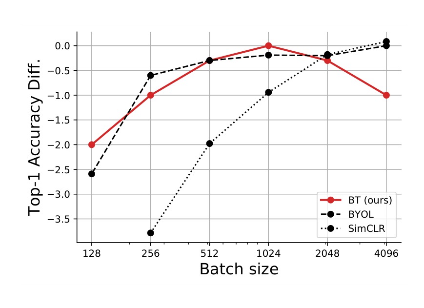
Figure 2. Effect of batch size. To compare the effect of the batch size across methods, for each method we report the difference between the top-1 accuracy at a given batch size and the best obtained accuracy among all batch size tested. BYOL: best accuracy is 72.5% for a batch size of 4096 (data from (Grill et al., 2020) fig. 3A). SIMCLR: best accuracy is 67.1% for a batch size of 4096 (data from (Chen et al., 2020a) fig. 9, model trained for 300 epochs). BARLOW TWINS: best accuracy is 71.7% for a batch size of 1024.
图 2:批次大小的影响。为了比较不同方法受批次大小的影响,对每种方法,我们报告给定批次大小下的 Top-1 准确率,与所有测试批次大小中得到的最佳准确率之差。BYOL:最佳准确率为 72.5%,对应批次大小 4096(数据来自 (Grill et al., 2020) 图 3A)。SIMCLR:最佳准确率为 67.1%,对应批次大小 4096(数据来自 (Chen et al., 2020a) 图 9,模型训练 300 个周期)。BARLOW TWINS:最佳准确率为 71.7%,对应批次大小 1024。
Effect of Removing Augmentations We find that our model is not robust to removing some types of data augmentations, like SIMCLR but unlike BYOL (Fig. 3). While this can be seen as a disadvantage of our method compared to BYOL, it can also be argued that the representations learned by our method are better controlled by the specific set of distortions used, as opposed to BYOL for which the invariances learned seem generic and intriguingly independent of the specific distortions used.
去掉增强的影响。我们发现,模型对去掉某些类型的数据增强并不稳健,这一点像 SIMCLR,而不像 BYOL(图 3)。虽然这可以看作我们的方法相对 BYOL 的一个缺点,但也可以说,我们的方法所学表征更好地受所用特定扰动集合的控制;相比之下,BYOL 学到的不变性显得更为一般,并且有意思的是,似乎并不依赖于所用的特定扰动。
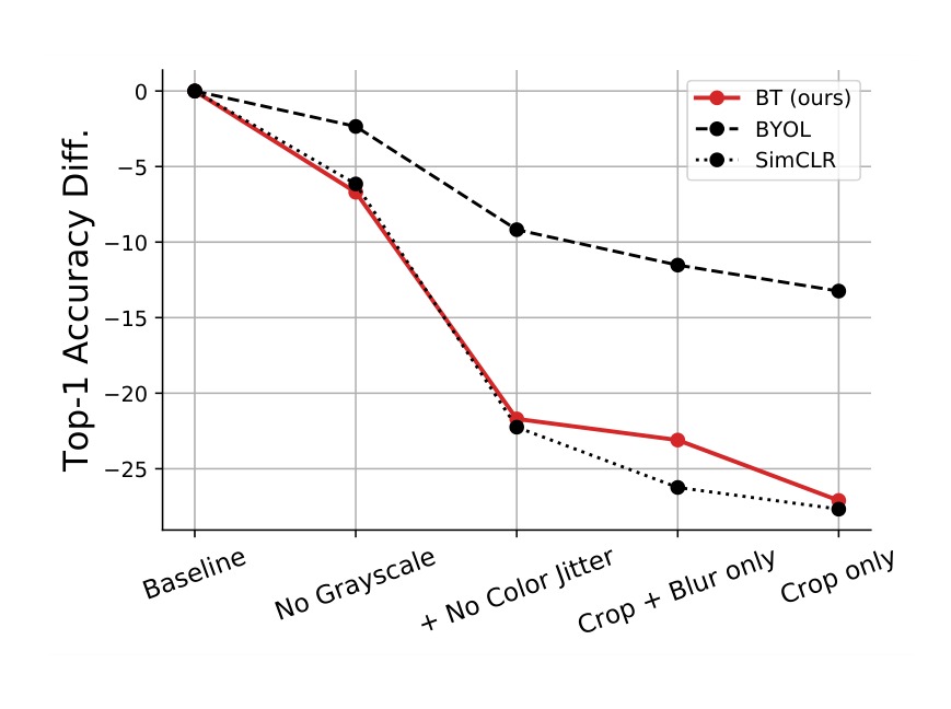
Figure 3. Effect of progressively removing data augmentations. Data for BYOL and SIMCLR (repro) is from (Grill et al., 2020) fig 3b.
图 3:逐步去掉数据增强的影响。BYOL 和 SIMCLR(复现)的数据来自 (Grill et al., 2020) 图 3b。
Projector Network Depth & Width For other SSL methods, such as BYOL and SIMCLR, the projector network drastically reduces the dimensionality of the ResNet output. In stark contrast, we find that BARLOW TWINS performs better when the dimensionality of the projector network output is very large. Other methods rapidly saturate when the dimensionality of the output increases, but our method keeps improving with all output dimensionality tested (Fig. 4). This result is quite surprising because the output of the ResNet is kept fixed to 2048, which acts as a dimensionality bottleneck in our model and sets the limit of the intrinsic dimensionality of the representation. In addition, similarly to other methods, we find that our model performs better when the projector network has more layers, with a saturation of the performance for 3 layers.
投影网络的深度与宽度。对 BYOL 和 SIMCLR 等其他自监督学习方法,投影网络会大幅降低 ResNet 输出的维度。与之形成鲜明对照的是,我们发现,当投影网络输出的维度非常大时,BARLOW TWINS 表现更好。其他方法在输出维度增大时很快饱和,而我们的方法在所测试的全部输出维度上持续提升(图 4)。这一结果相当出人意料,因为 ResNet 的输出仍固定为 2048,在我们的模型中构成维度瓶颈,并限定了表征的内在维度。此外,与其他方法类似,我们发现投影网络层数更多时模型表现更好,性能在 3 层时饱和。
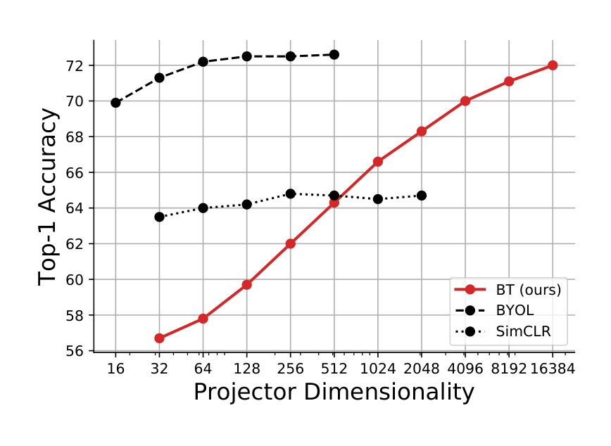
Figure 4. Effect of the dimensionality of the last layer of the projector network on performance. The parameter is kept fix for all dimensionalities tested. Data for SIMCLR is from (Chen et al., 2020a) fig 8; Data for BYOL is from (Grill et al., 2020) Table 14b.
图 4:投影网络最后一层维度对性能的影响。对所有测试的维度, 保持固定。SIMCLR 的数据来自 (Chen et al., 2020a) 图 8;BYOL 的数据来自 (Grill et al., 2020) 表 14b。
Breaking Symmetry Many SSL methods (e.g. BYOL, SIMSIAM, SWAV) rely on different symmetry-breaking mechanisms to avoid trivial solutions. Our loss function avoids these trivial solutions by construction, even in the case of symmetric networks. It is however interesting to ask whether breaking symmetry can further improve the performance of our network. Following SIMSIAM and BYOL, we experiment with adding a predictor network composed of 2 fully connected layers of size 8192 to one of the network (with batch normalization followed by a ReLU nonlinearity in the hidden layer) and/or a stop-gradient mechanism on the other network. We find that these asymmetries slightly decrease the performance of our network (see Table 6).
打破对称。许多自监督学习方法(例如 BYOL、SIMSIAM、SWAV)依靠不同的破对称机制来避免平凡解。我们的损失函数在构造上就避免了这些平凡解,即使网络是对称的。不过,仍然值得问:打破对称能否进一步提升我们网络的性能。沿用 SIMSIAM 和 BYOL,我们试验给其中一个网络加上由 2 个大小为 8192 的全连接层组成的预测网络(隐藏层中批归一化后接 ReLU 非线性),并且/或者在另一个网络上使用停止梯度机制。我们发现,这些不对称会略微降低网络的性能(见表 6)。
Table 6. Effect of asymmetric settings
| case | stop-gradient | predictor | Top-1 | Top-5 |
|---|---|---|---|---|
| Baseline | - | - | 71.4 | 90.2 |
| (a) | ✓ | - | 70.5 | 89.0 |
| (b) | - | ✓ | 70.2 | 89.0 |
| (c) | ✓ | ✓ | 61.3 | 83.5 |
表 6。不对称设置的影响
| 情形 | stop-gradient | predictor | Top-1 | Top-5 |
|---|---|---|---|---|
| Baseline | - | - | 71.4 | 90.2 |
| (a) | ✓ | - | 70.5 | 89.0 |
| (b) | - | ✓ | 70.2 | 89.0 |
| (c) | ✓ | ✓ | 61.3 | 83.5 |
BYOL with a larger projector/predictor/embedding For a fair comparison with BYOL, we also evaluated BYOL with a wider and/or deeper projector head (3-layer MLP), a wider and/or deeper predictor head, and a larger dimensionality of the embedding. BYOL did not improve under these conditions (see Table 7).
使用更大投影头 / 预测头 / 嵌入的 BYOL。为了与 BYOL 公平比较,我们也评估了使用更宽和/或更深投影头(3 层 MLP)、更宽和/或更深预测头,以及更大嵌入维度的 BYOL。在这些条件下,BYOL 并没有提升(见表 7)。
Table 7. Wider and/or deeper projector and predictor heads and larger dimensionality of the embedding did not improve the performance of BYOL.
| Projector | Predictor | Acc1 | Description |
|---|---|---|---|
| 4096-256 | 4096-256 | 74.1% | baseline |
| 4096-4096-256 | 4096-256 | 74.0% | 3 layer proj, 2 layer pred, 256-d repr. |
| 4096-4096-256 | 4096-4096-256 | 73.2% | 3 layer proj, 3 layer pred, 256-d repr. |
| 4096-4096-512 | 4096-512 | 73.7% | 3 layer proj, 2 layer pred, 512-d repr. |
| 4096-4096-512 | 4096-4096-512 | 73.2% | 3 layer proj, 3 layer pred, 512-d repr. |
| 8192-8192-8192 | 8192-8192 | 72.3% | same proj as BT, 2 layer pred, 8192-d repr. |
表 7。更宽和/或更深的投影头与预测头,以及更大的嵌入维度,并没有提升 BYOL 的性能。
| 投影头 | 预测头 | Acc1 | 说明 |
|---|---|---|---|
| 4096-256 | 4096-256 | 74.1% | 基线 |
| 4096-4096-256 | 4096-256 | 74.0% | 3 层投影头,2 层预测头,256 维表征 |
| 4096-4096-256 | 4096-4096-256 | 73.2% | 3 层投影头,3 层预测头,256 维表征 |
| 4096-4096-512 | 4096-512 | 73.7% | 3 层投影头,2 层预测头,512 维表征 |
| 4096-4096-512 | 4096-4096-512 | 73.2% | 3 层投影头,3 层预测头,512 维表征 |
| 8192-8192-8192 | 8192-8192 | 72.3% | 与 BT 相同的投影头,2 层预测头,8192 维表征 |
Sensitivity to . We also explored the sensitivity of BARLOW TWINS to the hyperparameter , which trades off the desiderata of invariance and informativeness of the embeddings. We find that BARLOW TWINS is not very sensitive to this hyperparameter (Fig. 5).
对 的敏感性。我们还探索了 BARLOW TWINS 对超参数 的敏感性,该参数权衡嵌入的不变性与信息量这两项要求。我们发现,BARLOW TWINS 对这一超参数并不十分敏感(图 5)。
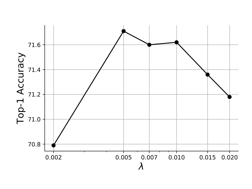
Figure 5. Sensitivity of BARLOW TWINS to the hyperparameter
图 5:BARLOW TWINS 对超参数 的敏感性
- Discussion
- 讨论
BARLOW TWINS learns self-supervised representations through a joint embedding of distorted images, with an objective function that maximizes similarity between the embedding vectors while reducing redundancy between their components. Our method does not require large batches of samples, nor does it require any particular asymmetry in the twin network structure. We discuss next the similarities and differences between our method and prior art, both from a conceptual and an empirical standpoint. For ease of comparison, all objective functions are recast with a common set of notations. The discussion ends with future directions.
BARLOW TWINS 通过对扰动图像做联合嵌入来学习自监督表征,其目标函数在最大化嵌入向量之间相似性的同时,减少它们各分量之间的冗余。我们的方法不需要大批次样本,也不需要孪生网络结构中任何特定的不对称。接下来,我们从概念和经验两方面讨论本方法与已有工作的异同。为便于比较,所有目标函数都改写成同一套记号。讨论以未来方向作结。
5.1. Comparison with Prior Art
5.1. 与已有工作的比较
infoNCE The INFONCE loss, where NCE stands for Noise-Contrastive Estimation (Gutmann & Hyvärinen, 2010), is a popular type of contrastive loss function used for self-supervised learning (e.g. (Chen et al., 2020a; He et al., 2019; Hénaff et al., 2019; Oord et al., 2018)). It can be instantiated as:
infoNCE。INFONCE 损失中的 NCE 代表噪声对比估计(Noise-Contrastive Estimation)(Gutmann & Hyvärinen, 2010),是自监督学习中一类常用的对比损失函数(例如 (Chen et al., 2020a; He et al., 2019; Hénaff et al., 2019; Oord et al., 2018))。它可以写成:
where and are the twin network outputs, indexes the sample in a batch, indexes the vector component of the output, and is a positive constant called temperature in analogy to statistical physics.
其中 和 是孪生网络的输出, 标示批次中的样本, 标示输出的向量分量, 是一个正常数,类比统计物理而称作温度。
For ready comparison, we rewrite BARLOW TWINS loss function with the same notations:
为便于直接比较,我们用同一套记号改写 BARLOW TWINS 的损失函数:
Both BARLOW TWINS' and INFONCE's objective functions have two terms, the first aiming at making the embeddings invariant to the distortions fed to the twin networks, the second aiming at maximizing the variability of the embedding learned. Another common point between the two losses is that they both rely on batch statistics to measure this variability. However, the INFONCE objective maximizes the variability of the embeddings by maximizing the pairwise distance between all pairs of samples, whereas our method does so by decorrelating the components of the embeddings vectors.
BARLOW TWINS 和 INFONCE 的目标函数都有两项:第一项旨在使嵌入对送入孪生网络的扰动保持不变,第二项旨在最大化所学嵌入的变异性。两个损失的另一个共同点是,它们都依靠批次统计量来度量这种变异性。不过,INFONCE 目标通过最大化所有样本对之间的成对距离来加大嵌入的变异性,而我们的方法则通过解除嵌入向量各分量之间的相关来做到这一点。
The contrastive term in INFONCE can be interpreted as a non-parametric estimation of the entropy of the distribution of embeddings (Wang & Isola, 2020). An issue that arises with non-parametric entropy estimators is that they are prone to the curse of dimensionality: they can only be estimated reliably in a low-dimensional setting, and they typically require a large number of samples.
INFONCE 中的对比项可以解释为对嵌入分布熵的非参数估计(Wang & Isola, 2020)。非参数熵估计器会遇到的一个问题是,它们容易受到维度灾难的影响:只有在低维设定下才能可靠估计,而且通常需要大量样本。
In contrast, our loss can be interpreted as a proxy entropy estimator of the distribution of embeddings under a Gaussian parametrization (see Appendix A). Thanks to this simplified parametrization, the variability of the embedding can be estimated from much fewer samples, and on very large-dimensional embeddings. Indeed, in the ablation studies that we perform, we find that (1) our method is robust to small batches unlike the popular INFONCE-based method SIMCLR, and (2) our method benefits from using very large dimensional embeddings, unlike INFONCE-based methods which do not see a benefit in increasing the dimensionality of the output.
相比之下,我们的损失可以解释为在高斯参数化下、对嵌入分布熵的一种代理估计(见附录 A)。得益于这一简化的参数化,嵌入的变异性可以从少得多的样本上估计,并且可以在非常高维的嵌入上估计。的确,在我们所做的消融研究中发现:(1) 与流行的基于 INFONCE 的方法 SIMCLR 不同,我们的方法对小批次是稳健的;(2) 我们的方法能从使用非常高维的嵌入中受益,而基于 INFONCE 的方法增加输出维度并看不到好处。
Our loss presents several other interesting differences with infoNCE:
我们的损失与 infoNCE 还有另外几点有意思的差异:
- In INFONCE, the embeddings are typically normalized along the feature dimension to compute a cosine similarity between embedded samples. We normalize the embeddings along the batch dimension instead.
- 在 INFONCE 中,嵌入通常沿特征维归一化,以便计算嵌入样本之间的余弦相似度。我们则沿批次维归一化嵌入。
- In our method, there is a parameter that trades off how much emphasis is put on the invariance term vs. the redundancy reduction term. This parameter can be interpreted as the trade-off parameter in the Information Bottleneck framework (see Appendix A). This parameter is not present in INFONCE.
- 在我们的方法中,有一个参数 ,用来权衡不变性项与冗余减少项各自的分量。该参数可以解释为信息瓶颈框架中的权衡参数(见附录 A)。INFONCE 中没有这一参数。
- INFONCE also has a hyperparameter, the temperature, which can be interpreted as the width of the kernel in a non-parametric kernel density estimation of entropy, and practically weighs the relative importance of the hardest negative samples present in the batch (Chen et al., 2020a).
- INFONCE 也有一个超参数,即温度,它可以解释为对熵做非参数核密度估计时核的宽度,并在实际上权衡批次中最难负样本的相对重要性(Chen et al., 2020a)。
A number of alternative methods to ours have been proposed to alleviate the reliance on large batches of the INFONCE loss. For example, MoCo (Chen et al., 2020b; He et al., 2019) builds a dynamic dictionary of negative samples with a queue and a moving-averaged encoder. This enables building a large and consistent dictionary on-the-fly that facilitates contrastive unsupervised learning. MoCo typically needs to store sample embeddings. In contrast, our method does not require such a large dictionary, since it works well with a relatively small batch size (e.g. 256).
已有若干替代方法被提出,以减轻 INFONCE 损失对大批次的依赖。例如,MoCo(Chen et al., 2020b; He et al., 2019)用一个队列和滑动平均编码器,构建负样本的动态词典。这能够即时建成一个规模大且一致的词典,从而便于对比无监督学习。MoCo 通常需要存储超过 个样本嵌入。相比之下,我们的方法不需要如此大的词典,因为它在相对较小的批次(例如 256)上就能表现良好。
Asymmetric Twins BOOTSTRAP-YOUR-OWN-LATENT (aka BYOL) (Grill et al., 2020) and SIMSIAM (Chen & He, 2020) are two recent methods which use a simple cosine similarity between twin embeddings as an objective function, without any contrastive term:
不对称孪生网络。BOOTSTRAP-YOUR-OWN-LATENT(又称 BYOL)(Grill et al., 2020)和 SIMSIAM(Chen & He, 2020)是两种近期方法,它们用孪生嵌入之间简单的余弦相似度作为目标函数,没有任何对比项:
Surprisingly, these methods successfully avoid trivial solutions by introducing some asymmetry in the architecture and learning procedure of the twin networks. For example, BYOL uses a predictor network which breaks the symmetry between the two networks, and also enforces an exponential moving average on the target network weights to slow down the progression of the weights on the target network. Combined together, these two mechanisms surprisingly avoid trivial solutions. The reasons behind this success are the subject of recent theoretical and empirical studies (Chen & He, 2020; Fetterman & Albrecht, 2020; Richemond et al., 2020; Tian et al., 2020). In particular, the ablation study (Chen & He, 2020) shows that the moving average is not necessary, but that stop-gradient on one of the branch and the presence of the predictor network are two crucial elements to avoid collapse. Other works show that batch normalization (Fetterman & Albrecht, 2020; Tian et al., 2020) or alternatively group normalization (Richemond et al., 2020) could play an important role in avoiding collapse.
出人意料的是,这些方法通过在孪生网络的结构和学习程序中引入某种不对称,成功地避免了平凡解。例如,BYOL 使用一个预测网络来打破两个网络之间的对称,并且对目标网络的权重施加指数滑动平均,以减缓目标网络权重的进展。这两种机制合在一起,竟然避免了平凡解。这一成功背后的原因,是近期理论和经验研究的对象(Chen & He, 2020; Fetterman & Albrecht, 2020; Richemond et al., 2020; Tian et al., 2020)。特别是,(Chen & He, 2020)的消融表明,滑动平均并不是必要的,但在其中一条分支上使用停止梯度,以及存在预测网络,是避免坍缩的两个关键因素。其他工作表明,批归一化(Fetterman & Albrecht, 2020; Tian et al., 2020),或者群归一化(Richemond et al., 2020),可能在避免坍缩中起重要作用。
Like our method, these asymmetric methods do not require large batches, since in their case there is no interaction between batch samples in the objective function.
与我们的方法一样,这些不对称方法也不需要大批次,因为在它们的情形中,目标函数里批次样本之间没有相互作用。
It should be noted however that these asymmetric methods cannot be described as the optimization of an overall learning objective. Instead, there exists trivial solutions to the learning objective that these methods avoid via particular implementation choices and/or the result of non-trivial learning dynamics. In contrast, our method avoids trivial solutions by construction, making our method conceptually simpler and more principled than these alternatives (until their principle is discovered, see (Tian et al., 2021) for an early attempt).
不过应当指出,这些不对称方法不能被描述成对某个总体学习目标的优化。相反,学习目标存在平凡解,而这些方法是通过特定的实现选择,和/或不平凡的学习动力学结果,来避开这些解的。相比之下,我们的方法在构造上就避免了平凡解,因而在概念上比这些替代方法更简单,也更有原则(直到它们的原则被发现为止,早期尝试见 (Tian et al., 2021))。
Whitening In a concurrent work, (Ermolov et al., 2020) propose W-MSE. Acting on the embeddings from identical twin networks, this method performs a differentiable whitening operation (via Cholesky decomposition) of each batch of embeddings before computing a simple cosine similarity between the whitened embeddings of the twin networks. In contrast, the redundancy reduction term in our loss encourages the whitening of the batch embeddings as a soft constraint. The current W-MSE model achieves 66.3% top-1 accuracy on the Imagenet linear evaluation benchmark. It is an interesting direction for future studies to determine whether improved versions of this hard-whitening strategy could also lead to state-of-the-art results on these large-scale computer vision benchmarks.
白化。在一项同时期的工作中,(Ermolov et al., 2020)提出了 W-MSE。该方法作用于来自相同孪生网络的嵌入,对每个批次的嵌入做可微白化操作(通过 Cholesky 分解),然后再计算孪生网络白化嵌入之间简单的余弦相似度。相比之下,我们损失中的冗余减少项,是把批次嵌入的白化作为软约束来鼓励的。当前的 W-MSE 模型在 ImageNet 线性评估基准上取得 66.3% 的 Top-1 准确率。改进后的硬白化策略能否也在这些大规模计算机视觉基准上达到最先进结果,是值得未来研究的一个方向。
Clustering These methods, such as DEEPCLUSTER (Caron et al., 2018), SWAV (Caron et al., 2020), SELA (Asano et al., 2020), perform contrastive-like comparisons without the requirement to compute all pairwise distances. Specifically, these methods simultaneously cluster the data while enforcing consistency between cluster assignments produced for different distortions of the same image, instead of comparing features directly as in contrastive learning. Clustering methods are also prone to collapse, e.g., empty clusters in k-means and avoiding them relies on careful implementation details. Online clustering methods like SWAV can be trained with large and small batches but require storing features when the number of clusters is much larger than the batch size. Clustering methods can also be combined with contrastive learning (Li et al., 2021) to prevent collapse.
聚类。这类方法,例如 DEEPCLUSTER(Caron et al., 2018)、SWAV(Caron et al., 2020)、SELA(Asano et al., 2020),进行类似对比的比较,但不必计算所有成对距离。具体而言,这些方法在对数据聚类的同时,强制同一图像不同扰动所产生的聚类分配保持一致,而不是像对比学习那样直接比较特征。聚类方法也容易坍缩,例如 k-means 中的空簇,避开它们要靠仔细的实现细节。像 SWAV 这样的在线聚类方法可以用大批次和小批次训练,但当簇数远大于批次大小时,需要存储特征。聚类方法也可以与对比学习结合(Li et al., 2021),以防止坍缩。
Noise As Targets This method (Bojanowski & Joulin, 2017) learns to map samples to fixed random targets on the unit sphere, which can be interpreted as a form of whitening. This objective uses a single network, and hence does not leverage the distortions induced by twin networks. Pre-defining random targets might limit the flexibility of the representation that can be learned.
以噪声为目标。该方法(Bojanowski & Joulin, 2017)学习把样本映射到单位球面上固定的随机目标,这可以解释为一种白化。这一目标只使用单个网络,因而没有利用孪生网络所引入的扰动。预先定义随机目标,可能会限制所能学习的表征的灵活性。
IMAX In the early days of SSL, (Becker & Hinton, 1992; Zemel & Hinton, 1990) proposed a loss function between twin networks given by:
IMAX。在自监督学习的早期,(Becker & Hinton, 1992; Zemel & Hinton, 1990)提出了孪生网络之间的如下损失函数:
where denotes the determinant of a matrix, is the covariance matrix of the difference of the outputs of the twin networks and the covariance of the sum of these outputs. It can be shown that this objective maximizes the information between the twin network representations under the assumptions that the two representations are noisy versions of the same underlying Gaussian signal, and that the noise is independant, additive and Gaussian. This objective is similar to ours in the sense that there is one term that encourages the two representations to be similar and another term that encourages the units to be decorrelated. However, unlike IMAX, our objective is not directly an information quantity, and we have an extra trade-off parameter that trades off the two terms of our loss. The IMAX objective was used in early work so it is not clear whether it can scale to large computer vision tasks. Our attempts to make it work on ImageNet were not successful.
其中 表示矩阵的行列式, 是孪生网络输出之差的协方差矩阵, 是这些输出之和的协方差。可以证明,在两个表征是同一潜在高斯信号的含噪版本、且噪声独立、加性且为高斯的假定下,这一目标最大化孪生网络表征之间的信息。该目标与我们的目标相似之处在于:有一项鼓励两个表征相似,另一项鼓励各单元去相关。不过,与 IMAX 不同,我们的目标并不是直接的信息量,并且我们还有一个额外的权衡参数 来权衡损失中的两项。IMAX 目标用在早期工作中,因此尚不清楚它能否扩展到大型计算机视觉任务。我们试图让它在 ImageNet 上奏效,但没有成功。
5.2. Future Directions
5.2. 未来方向
We observe a steady improvement of the performance of our method as we increase the dimensionality of the embeddings (i.e. of the last layer of the projector network). This intriguing result is in stark contrast with other popular methods for SSL, such as SIMCLR (Chen et al., 2020a) and BYOL (Grill et al., 2020), for which increasing the dimensionality of the embeddings rapidly saturates performance. It is a promising avenue to continue this exploration for even higher dimensional embeddings (), but this would require the development of new methods or alternative hardware to accommodate the memory requirements of operating on such large embeddings.
我们观察到,随着嵌入维度(即投影网络最后一层的维度)增加,本方法的性能稳步提升。这一有意思的结果,与 SIMCLR(Chen et al., 2020a)和 BYOL(Grill et al., 2020)等其他流行的自监督学习方法形成鲜明对照:对后者而言,增大嵌入维度后性能很快饱和。继续把这一探索推向更高维的嵌入()是一条有前景的路线,但这需要发展新的方法或改用其他硬件,以应对在如此大的嵌入上运算的内存需求。
Our method is just one possible instanciation of the Information Bottleneck principle applied to SSL. We believe that further refinements of the proposed loss function and algorithm could lead to more efficient solutions and even better performances. For example, the redundancy reduction term is currently computed from the off-diagonal terms of the cross-correlation matrix between the twin network embeddings, but alternatively it could be computed from the off-diagonal terms of the auto-correlation matrix of a single network's embedding. Our preliminary analyses seem to indicate that this alternative leads to similar performances (not shown). A modified loss could also be applied to the (unnormalized) cross-covariance matrix instead of the (normalized) cross-correlation matrix (see Ablations for preliminary analyses).
我们的方法只是把信息瓶颈原则用于自监督学习的一种可能实例。我们相信,对所提损失函数和算法做进一步改进,有可能得到更高效的方案,以及更好的性能。例如,冗余减少项目前是由孪生网络嵌入之间互相关矩阵的非对角项计算的,但也可以改由单个网络嵌入的自相关矩阵的非对角项来计算。我们的初步分析似乎表明,这一替代方案会带来相近的性能(未展示)。也可以把修改后的损失作用于(未归一化的)互协方差矩阵,而不是(归一化的)互相关矩阵(初步分析见消融实验)。
Acknowledgements
致谢
We thank Pascal Vincent, Yubei Chen and Samuel Ocko for helpful insights on the mathematical connection to the infoNCE loss, Robert Geirhos and Adrien Bardes for extra analyses not included in the manuscript and Xinlei Chen, Mathilde Caron, Armand Joulin, Reuben Feinman and Ulisse Ferrari for useful comments on the manuscript.
我们感谢 Pascal Vincent、Yubei Chen 和 Samuel Ocko 就与 infoNCE 损失的数学联系提供的有益见解,感谢 Robert Geirhos 和 Adrien Bardes 所做的、未收入本稿的额外分析,并感谢 Xinlei Chen、Mathilde Caron、Armand Joulin、Reuben Feinman 和 Ulisse Ferrari 对稿件的有用意见。
References
参考文献
Asano, Y. M., Rupprecht, C., and Vedaldi, A. Self-labelling via simultaneous clustering and representation learning. International Conference on Learning Representations (ICLR), 2020.
Ballé, J., Laparra, V., and Simoncelli, E. P. End-to-end Optimized Image Compression. In International Conference on Learning Representations (ICLR), 2017.
Barlow, H. Redundancy reduction revisited. Network (Bristol, England), 12(3):241–253, August 2001. ISSN 0954-898X.
Barlow, H. B. Possible Principles Underlying the Transformations of Sensory Messages. In Sensory Communication. The MIT Press, 1961.
Becker, S. and Hinton, G. E. Self-organizing neural network that discovers surfaces in random-dot stereograms. Nature, 355(6356):161–163, January 1992.
Bojanowski, P. and Joulin, A. Unsupervised learning by predicting noise. In Proceedings of the International Conference on Machine Learning (ICML), 2017.
Caron, M., Bojanowski, P., Joulin, A., and Douze, M. Deep clustering for unsupervised learning of visual features. In Proceedings of the European Conference on Computer Vision (ECCV), 2018.
Caron, M., Misra, I., Mairal, J., Goyal, P., Bojanowski, P., and Joulin, A. Unsupervised learning of visual features by contrasting cluster assignments. In NeurIPS, 2020.
Chen, T., Kornblith, S., Norouzi, M., and Hinton, G. A simple framework for contrastive learning of visual representations. arXiv preprint arXiv:2002.05709, 2020a.
Chen, X. and He, K. Exploring simple siamese representation learning. arXiv preprint arXiv:2011.10566, 2020.
Chen, X., Fan, H., Girshick, R., and He, K. Improved baselines with momentum contrastive learning. arXiv preprint arXiv:2003.04297, 2020b.
Deco, G. and Parra, L. Non-linear Feature Extraction by Redundancy Reduction in an Unsupervised Stochastic Neural Network. Neural Networks, 10(4):683–691, June 1997. ISSN 0893-6080. doi: 10.1016/S0893-6080(96)00110-4.
Deng, J., Dong, W., Socher, R., Li, L.-J., Li, K., and Fei-Fei, L. Imagenet: A large-scale hierarchical image database. In Proceedings of the Conference on Computer Vision and Pattern Recognition (CVPR), 2009.
Ermolov, A., Siarohin, A., Sangineto, E., and Sebe, N. Whitening for Self-Supervised Representation Learning. arXiv preprint arXiv:2007.06346, 2020.
Everingham, M., Van Gool, L., Williams, C. K., Winn, J., and Zisserman, A. The pascal visual object classes (voc) challenge. International journal of computer vision, 88(2):303–338, 2010.
Fetterman, A. and Albrecht, J. Understanding self-supervised and contrastive learning with “Bootstrap Your Own Latent” (BYOL). Untitled AI, August 2020.
Földiák, P. Forming sparse representations by local anti-Hebbian learning. Biological Cybernetics, 64(2):165–170, December 1990. ISSN 1432-0770. doi: 10.1007/BF02331346.
Goyal, P., Mahajan, D., Gupta, A., and Misra, I. Scaling and benchmarking self-supervised visual representation learning. Proceedings of the International Conference on Computer Vision (ICCV), 2019.
Grill, J.-B., Strub, F., Altché, F., Tallec, C., Richemond, P. H., Buchatskaya, E., Doersch, C., Pires, B. A., Guo, Z. D., Azar, M. G., et al. Bootstrap your own latent: A new approach to self-supervised learning. In NeurIPS, 2020.
Gutmann, M. and Hyvärinen, A. Noise-contrastive estimation: A new estimation principle for unnormalized statistical models. In Proceedings of the Thirteenth International Conference on Artificial Intelligence and Statistics. JMLR Workshop and Conference Proceedings, 2010.
Hadsell, R., Chopra, S., and LeCun, Y. Dimensionality reduction by learning an invariant mapping. In Proceedings of the Conference on Computer Vision and Pattern Recognition (CVPR), 2006.
He, K., Zhang, X., Ren, S., and Sun, J. Deep residual learning for image recognition. In Proceedings of the Conference on Computer Vision and Pattern Recognition (CVPR), 2016.
He, K., Gkioxari, G., Dollár, P., and Girshick, R. Mask r-cnn. In Proceedings of the International Conference on Computer Vision (ICCV), 2017.
He, K., Fan, H., Wu, Y., Xie, S., and Girshick, R. Momentum contrast for unsupervised visual representation learning. arXiv preprint arXiv:1911.05722, 2019.
Hénaff, O. J., Razavi, A., Doersch, C., Eslami, S., and Oord, A. v. d. Data-efficient image recognition with contrastive predictive coding. arXiv preprint arXiv:1905.09272, 2019.
Li, Y., Hu, P., Liu, Z., Peng, D., Zhou, J. T., and Peng, X. Contrastive clustering. In AAAI, 2021.
Lin, T.-Y., Maire, M., Belongie, S., Hays, J., Perona, P., Ramanan, D., Dollár, P., and Zitnick, C. L. Microsoft coco: Common objects in context. In Proceedings of the European Conference on Computer Vision (ECCV), 2014.
Lindsey, J., Ocko, S. A., Ganguli, S., and Deny, S. A unified theory of early visual representations from retina to cortex through anatomically constrained deep CNNs. In ICLR, 2020.
Linsker, R. Self-organization in a perceptual network. Computer, 21(3):105–117, March 1988. ISSN 1558-0814. doi: 10.1109/2.36. Conference Name: Computer.
Loshchilov, I. and Hutter, F. Sgdr: Stochastic gradient descent with warm restarts. arXiv preprint arXiv:1608.03983, 2016.
Misra, I. and van der Maaten, L. Self-supervised learning of pretext-invariant representations. arXiv preprint arXiv:1912.01991, 2019.
Ocko, S., Lindsey, J., Ganguli, S., and Deny, S. The emergence of multiple retinal cell types through efficient coding of natural movies. In NeurIPS, 2018.
Oord, A. v. d., Li, Y., and Vinyals, O. Representation learning with contrastive predictive coding. arXiv preprint arXiv:1807.03748, 2018.
Redlich, A. N. Redundancy Reduction as a Strategy for Unsupervised Learning. Neural Computation, 5(2):289–304, March 1993a. ISSN 0899-7667. doi: 10.1162/neco.1993.5.2.289. Conference Name: Neural Computation.
Redlich, A. N. Supervised Factorial Learning. Neural Computation, 5(5):750–766, September 1993b. ISSN 0899-7667, 1530-888X. doi: 10.1162/neco.1993.5.5.750.
Ren, S., He, K., Girshick, R., and Sun, J. Faster r-cnn: Towards real-time object detection with region proposal networks. In Advances in Neural Information Processing Systems (NeurIPS), 2015.
Richemond, P. H., Grill, J.-B., Altché, F., Tallec, C., Strub, F., Brock, A., Smith, S., De, S., Pascanu, R., Piot, B., and Valko, M. BYOL works even without batch statistics. arXiv preprint arXiv:2010.10241, 2020.
Schmidhuber, J., Eldracher, M., and Foltin, B. Semilinear Predictability Minimization Produces Well-Known Feature Detectors. Neural Computation, 8(4):773–786, May 1996. ISSN 0899-7667. doi: 10.1162/neco.1996.8.4.773. Conference Name: Neural Computation.
Schwartz, O. and Simoncelli, E. P. Natural signal statistics and sensory gain control. Nature Neuroscience, 4(8):819–825, August 2001. ISSN 1546-1726. doi: 10.1038/90526. Number: 8 Publisher: Nature Publishing Group.
Tian, Y., Yu, L., Chen, X., and Ganguli, S. Understanding Self-supervised Learning with Dual Deep Networks. arXiv preprint arXiv:2010.00578, 2020.
Tian, Y., Chen, X., and Ganguli, S. Understanding self-supervised Learning Dynamics without Contrastive Pairs. arXiv:2102.06810 [cs], February 2021. arXiv: 2102.06810.
Tishby, N. and Zaslavsky, N. Deep Learning and the Information Bottleneck Principle. arXiv preprint arXiv:1503.02406, 2015.
Tishby, N., Pereira, F. C., and Bialek, W. The information bottleneck method. arXiv preprint arXiv:physics/0004057, 2000.
Van Horn, G., Mac Aodha, O., Song, Y., Cui, Y., Sun, C., Shepard, A., Adam, H., Perona, P., and Belongie, S. The inaturalist species classification and detection dataset. In Proceedings of the Conference on Computer Vision and Pattern Recognition (CVPR), 2018.
Wang, T. and Isola, P. Understanding Contrastive Representation Learning through Alignment and Uniformity on the Hypersphere. arXiv preprint arXiv:2005.10242, 2020.
Wu, Y., Kirillov, A., Massa, F., Lo, W.-Y., and Girshick, R. Detectron2. https://github.com/facebookresearch/detectron2, 2019.
You, Y., Gitman, I., and Ginsburg, B. Large batch training of convolutional networks. arXiv preprint arXiv:1708.03888, 2017.
Zemel, R. and Hinton, G. E. Discovering viewpoint-invariant relationships that characterize objects. In NeurIPS, 1990.
Zhai, X., Oliver, A., Kolesnikov, A., and Beyer, L. S4l: Self-supervised semi-supervised learning. In Proceedings of the IEEE/CVF International Conference on Computer Vision, pp. 1476–1485, 2019.
Zhou, B., Lapedriza, A., Xiao, J., Torralba, A., and Oliva, A. Learning deep features for scene recognition using places database. In Advances in Neural Information Processing Systems (NeurIPS), 2014.