Guiding a Diffusion Model with a Bad Version of Itself

用自身较差版本引导扩散模型

Tero Karras Affiliation:  NVIDIA    Miika Aittala Affiliation:  NVIDIA    Tuomas Kynkäänniemi Affiliation:  Aalto University    Jaakko Lehtinen Affiliation:  NVIDIA, Aalto University    Timo Aila Affiliation:  NVIDIA    Samuli Laine Affiliation:  NVIDIA

Abstract

摘要

The primary axes of interest in image-generating diffusion models are image quality, the amount of variation in the results, and how well the results align with a given condition, e.g., a class label or a text prompt. The popular classifier-free guidance approach uses an unconditional model to guide a conditional model, leading to simultaneously better prompt alignment and higher-quality images at the cost of reduced variation. These effects seem inherently entangled, and thus hard to control. We make the surprising observation that it is possible to obtain disentangled control over image quality without compromising the amount of variation by guiding generation using a smaller, less-trained version of the model itself rather than an unconditional model. This leads to significant improvements in ImageNet generation, setting record FIDs of 1.01 for $64{\times}64$ and 1.25 for $512{\times}512$, using publicly available networks. Furthermore, the method is also applicable to unconditional diffusion models, drastically improving their quality.

图像生成扩散模型的主要关注轴包括图像质量、结果多样性，以及结果与给定条件（如类别标签或文本提示）的对齐程度。流行的无分类器引导（classifier-free guidance）用无条件模型去引导条件模型，能同时提升提示对齐与图像质量，却以牺牲多样性为代价。这些效应似乎纠缠在一起，因而难以分别控制。我们观察到一个出人意料的现象：不必用无条件模型，而用主模型自身一个更小、训练更不充分的版本来引导生成，就能在不牺牲多样性的前提下，单独调控图像质量。这在 ImageNet 生成上带来显著提升，使用公开可用网络分别把 $64{\times}64$ 与 $512{\times}512$ 的 FID 刷到 1.01 与 1.25 的纪录。此外，该方法同样适用于无条件扩散模型，并大幅提升其质量。

1 Introduction

1 引言

Denoising diffusion models [15, 46, 47, 48, 49] generate synthetic images by reversing a stochastic corruption process. Essentially, an image is revealed from pure noise by denoising it little by little in successive steps. A neural network that implements the denoiser (equivalently [53], the score function [20]) is a central design element, and various architectures have been proposed (e.g., [2, 7, 9, 19, 21, 24, 38]). Equally important are the details of the multi-step denoising process that corresponds mathematically to solving an ordinary [35, 47] or a stochastic [49] differential equation, for which many different parameterizations, solvers, and step schedules have been evaluated [22, 23, 30, 43, 57]. To control the output image, the denoiser is typically conditioned on a class label, an embedding of a text prompt, or some other form of conditioning input [36, 41, 45, 56].

去噪扩散模型 [15, 46, 47, 48, 49] 通过反转随机腐蚀过程来生成合成图像。本质上，图像是从纯噪声中逐步去噪、一点一点显露出来的。实现去噪器（等价地 [53]，即得分函数 [20]）的神经网络是核心设计要素，已有多种架构被提出（例如 [2, 7, 9, 19, 21, 24, 38]）。同样重要的是多步去噪过程的细节：它在数学上对应求解常微分方程 [35, 47] 或随机微分方程 [49]，人们已评估过许多参数化、求解器与步长安排 [22, 23, 30, 43, 57]。为控制输出图像，去噪器通常以类别标签、文本提示的嵌入或其他形式的条件输入为条件 [36, 41, 45, 56]。

The training objective of a diffusion model aims to cover the entire (conditional) data distribution. This causes problems in low-probability regions: The model gets heavily penalized for not representing them, but it does not have enough data to learn to generate good images corresponding to them. Classifier-free guidance (CFG) [16] has become the standard method for “lowering the sampling temperature”, i.e., focusing the generation on well-learned high-probability regions. By training a denoiser network to operate in both conditional and unconditional setting, the sampling process can be steered away from the unconditional result — in effect, the unconditional generation task specifies a result to avoid. This results in better prompt alignment and improved image quality, where the former effect is due to CFG implicitly raising the conditional part of the probability density to a power greater than one [10].

扩散模型的训练目标旨在覆盖整个（条件）数据分布。这在低概率区域会带来麻烦：模型若不表征这些区域会受到重罚，却又没有足够数据学会生成对应的好图像。无分类器引导（CFG） [16] 已成为「降低采样温度」、即把生成聚焦到学得较好的高概率区域的标准方法。通过让去噪网络同时在条件与无条件下工作，采样过程可被推离无条件结果——无条件生成任务实质上指定了一个要避开的结果。这带来更好的提示对齐与更高的图像质量；其中对齐效果来自 CFG 隐式地把条件部分的概率密度抬到大于一的幂次 [10]。

However, CFG has drawbacks that limit its usage as a general low-temperature sampling method. First, it is applicable only for conditional generation, as the guidance signal is based on the difference between conditional and unconditional denoising results. Second, because the unconditional and conditional denoisers are trained to solve a different task, the sampling trajectory can overshoot the desired conditional distribution, which leads to skewed and often overly simplified image compositions [27]. Finally, the prompt alignment and quality improvement effects cannot be controlled separately, and it remains unclear how exactly they relate to each other.

然而 CFG 有若干缺陷，限制了它作为通用低温采样方法的用途。首先，它只适用于条件生成，因为引导信号依赖条件与无条件去噪结果之差。其次，无条件与条件去噪器被训练去解决不同任务，采样轨迹可能冲过期望的条件分布，导致构图偏斜、往往过度简化 [27]。最后，提示对齐与质量提升无法分开控制，二者究竟如何关联也仍不清楚。

In this paper, we provide new insights into why CFG improves image quality and show how this effect can be separated out into a novel method that we call autoguidance. Our method does not suffer from the task discrepancy problem because we use an inferior version of the main model itself as the guiding model, with unchanged conditioning. This guiding model can be obtained by simply limiting, e.g., model capacity and/or training time. We validate the effectiveness of autoguidance in various synthetic test cases as well as in practical image synthesis in class-conditional and text-conditional settings. In addition, our method enables guidance for unconditional synthesis. In quantitative tests, the generated image distributions are improved considerably when measured using FID [13] and FDDINOv2 [51] metrics, setting new records in ImageNet-512 and ImageNet-64 generation.

本文给出新的洞见：为何 CFG 能提升图像质量，以及如何把这一效应分离成我们称为 autoguidance（自引导）的新方法。由于我们用主模型自身的较差版本作引导模型、且条件保持不变，该方法不受任务不一致问题的困扰。引导模型只需限制模型容量与/或训练时间即可得到。我们在多种合成测试以及类别条件、文本条件等实用图像合成设定中验证了自引导的有效性；此外，它还能为无条件合成提供引导。定量测试中，生成图像分布在 FID [13] 与 FDDINOv2 [51] 上显著改善，并在 ImageNet-512 与 ImageNet-64 上创下新纪录。

Our implementation and pre-trained models are available at https://github.com/NVlabs/edm2

实现与预训练模型见 https://github.com/NVlabs/edm2

2 Background

2 背景

Denoising diffusion.

Denoising diffusion generates samples from a distribution $p_{\text{data}}(\mathbf{x})$ by iteratively denoising a sample of pure white noise, such that a noise-free random data sample is gradually revealed [15]. The idea is to consider heat diffusion of $p_{\text{data}}(\mathbf{x})$ into a sequence of increasingly smoothed densities $p(\mathbf{x};\sigma)=p_{\text{data}}(\mathbf{x})\ast\mathcal{N}(\mathbf{x};\mathbf{0},\sigma^{2}\mathbf{I})$. For a large enough $\sigma_{\text{max}}$, we have $p(\mathbf{x};\sigma_{\text{max}})\approx\mathcal{N}(\mathbf{x};\mathbf{0},\sigma_{\text{max}}^{2}\mathbf{I})$, from which we can trivially sample by drawing normally distributed white noise. The resulting sample is then evolved backward towards low noise levels by a probability flow ODE [23, 47, 49]

去噪扩散。

去噪扩散通过迭代去噪纯白噪声样本，从分布 $p_{\text{data}}(\mathbf{x})$ 中采样，从而逐步揭示无噪声的随机数据样本 [15]。思路是把 $p_{\text{data}}(\mathbf{x})$ 的热扩散写成一串越来越平滑的密度 $p(\mathbf{x};\sigma)=p_{\text{data}}(\mathbf{x})\ast\mathcal{N}(\mathbf{x};\mathbf{0},\sigma^{2}\mathbf{I})$。对足够大的 $\sigma_{\text{max}}$，有 $p(\mathbf{x};\sigma_{\text{max}})\approx\mathcal{N}(\mathbf{x};\mathbf{0},\sigma_{\text{max}}^{2}\mathbf{I})$，可直接抽取正态白噪声作为样本。随后用概率流 ODE [23, 47, 49] 把该样本向低噪声水平反向演化

$$\displaystyle\mathrm{d}\mathbf{x}_{\sigma} \\ \displaystyle\,=\,-\sigma\smash{\nabla_{\hskip-0.98329pt\mathbf{x}_{\sigma}}\hskip-2.5pt}\log p(\mathbf{x}_{\sigma};\sigma)~\mathrm{d}\sigma \tag{1}$$

that maintains the property $\mathbf{x}_{\sigma}\sim p(\mathbf{x}_{\sigma};\sigma\big)$ for every $\sigma\in[0,\sigma_{\text{max}}]$. Upon reaching $\sigma=0$, we obtain $\mathbf{x}_{0}\sim p(\mathbf{x}_{0};0)=p_{\text{data}}(\mathbf{x}_{0})$ as desired.

该方程对每个 $\sigma\in[0,\sigma_{\text{max}}]$ 保持性质 $\mathbf{x}_{\sigma}\sim p(\mathbf{x}_{\sigma};\sigma)$。到达 $\sigma=0$ 时，即得期望的 $\mathbf{x}_{0}\sim p(\mathbf{x}_{0};0)=p_{\text{data}}(\mathbf{x}_{0})$。

In practice, the ODE is solved numerically by stepping along the trajectory defined by Equation 1. This requires evaluating the so-called score function [20] $\smash{\nabla_{\hskip-0.98329pt\mathbf{x}}\hskip-0.50003pt}\log p(\mathbf{x};\sigma)$ for a given sample $\mathbf{x}$ and noise level $\sigma$ at each step. Rather surprisingly, we can approximate this vector using a neural network $D_{\theta}(\mathbf{x};\sigma)$ parameterized by weights $\theta$ trained for the denoising task

实践中，沿式 1 定义的轨迹数值求解 ODE。每一步都需要在给定样本 $\mathbf{x}$ 与噪声水平 $\sigma$ 处评估所谓得分函数 [20] $\smash{\nabla_{\hskip-0.98329pt\mathbf{x}}\hskip-0.50003pt}\log p(\mathbf{x};\sigma)$。相当出人意料的是，可用参数为 $\theta$、为去噪任务训练的神经网络 $D_{\theta}(\mathbf{x};\sigma)$ 来近似该向量

$$\displaystyle\theta \\ \displaystyle\,=\,\argmin_{\theta}\mathbb{E}_{\mathbf{y}\sim p_{\text{data}},\sigma\sim p_{\text{train}},\mathbf{n}\sim\mathcal{N}(\mathbf{0},\sigma^{2}\mathbf{I})}\lVert D_{\theta}(\mathbf{y}+\mathbf{n};\sigma)-\boldsymbol{y}\rVert^{2}_{2}\text{,} \tag{2}$$

where $p_{\text{train}}$ controls the noise level distribution during training. Given $D_{\theta}$, we can estimate $\smash{\nabla_{\hskip-0.98329pt\mathbf{x}}\hskip-0.50003pt}\log p(\mathbf{x};\sigma)\approx(D_{\theta}(\mathbf{x};\sigma)-\mathbf{x})/\sigma^{2}$, up to approximation errors due to, e.g., finite capacity or training time [23, 53]. As such, we are free to interpret the network as predicting either a denoised sample or a score vector, whichever is more convenient for the analysis at hand. Many reparameterizations and practical ODE solvers are possible, as enumerated by Karras et al. [23]. We follow their recommendations, including the schedule $\sigma(t)=t$ that lets us parameterize the ODE directly via noise level $\sigma$ instead of a separate time variable $t$.

其中 $p_{\text{train}}$ 控制训练时的噪声水平分布。给定 $D_{\theta}$，可估计 $\smash{\nabla_{\hskip-0.98329pt\mathbf{x}}\hskip-0.50003pt}\log p(\mathbf{x};\sigma)\approx(D_{\theta}(\mathbf{x};\sigma)-\mathbf{x})/\sigma^{2}$，近似误差来自有限容量或训练时间等 [23, 53]。因此，把网络解读成预测去噪样本或得分向量均可，视分析方便而定。Karras 等人 [23] 列举了许多重参数化与实用 ODE 求解器；我们沿用其建议，包括调度 $\sigma(t)=t$，从而可直接用噪声水平 $\sigma$ 参数化 ODE，而不另设时间变量 $t$。

In most applications, each data sample $\mathbf{x}$ is associated with a label $\mathbf{c}$, representing, e.g., a class index or a text prompt. At generation time, we control the outcome by choosing a label $\mathbf{c}$ and seeking a sample from the conditional distribution $p(\mathbf{x}|\mathbf{c};\sigma)$ with $\sigma=0$. In practice, this is achieved by training a denoiser network $D_{\theta}(\mathbf{x};\sigma,\mathbf{c})$ that accepts $\mathbf{c}$ as an additional conditioning input.

多数应用中，每个数据样本 $\mathbf{x}$ 关联一个标签 $\mathbf{c}$，例如类别索引或文本提示。生成时选定标签 $\mathbf{c}$，并寻求 $\sigma=0$ 时条件分布 $p(\mathbf{x}|\mathbf{c};\sigma)$ 的样本。实践上，通过训练接受 $\mathbf{c}$ 作为额外条件输入的去噪网络 $D_{\theta}(\mathbf{x};\sigma,\mathbf{c})$ 实现。

Classifier-free guidance.

For complex visual datasets, the generated images often fail to reproduce the clarity of the training images due to approximation errors made by finite-capacity networks. A broadly used trick called classifier-free guidance (CFG) [16] pushes the samples towards higher likelihood of the class label, sacrificing variety for “more canonical” images that the network appears to be better capable of handling.

无分类器引导。

对复杂视觉数据集，生成图像往往因有限容量网络的近似误差而无法再现训练图像的清晰度。广泛使用的技巧 无分类器引导（CFG） [16] 把样本推向类别标签更高似然的区域，牺牲多样性以换取网络更擅长处理的「更典型」图像。

In a general setting, guidance in a diffusion model involves two denoiser networks $D_{0}(\mathbf{x};\sigma,\mathbf{c})$ and $D_{1}(\mathbf{x};\sigma,\mathbf{c})$. The guiding effect is achieved by extrapolating between the two denoising results by a factor $w$:

一般设定下，扩散模型中的引导涉及两个去噪网络 $D_{0}(\mathbf{x};\sigma,\mathbf{c})$ 与 $D_{1}(\mathbf{x};\sigma,\mathbf{c})$。引导效果通过对两路去噪结果按因子 $w$ 外推 实现：

$$\displaystyle D_{w}(\mathbf{x};\sigma,\mathbf{c}) \\ \displaystyle\,=\,wD_{1}(\mathbf{x};\sigma,\mathbf{c})+(1-w)D_{0}(\mathbf{x};\sigma,\mathbf{c})\text{.} \tag{3}$$

Trivially, setting $w=0$ or $w=1$ recovers the output of $D_{0}$ and $D_{1}$, respectively, while choosing $w>1$ over-emphasizes the output of $D_{1}$. Recalling the equivalence of denoisers and scores [53], we can write

显然，$w=0$ 或 $w=1$ 分别恢复 $D_{0}$ 与 $D_{1}$ 的输出，而 $w>1$ 则过度强调 $D_{1}$。回忆去噪器与得分的等价性 [53]，可写成

$$\displaystyle D_{w}(\mathbf{x};\sigma,\mathbf{c}) \\ \displaystyle\,\approx\,\mathbf{x}+\sigma^{2}\smash{\nabla_{\hskip-0.98329pt\mathbf{x}}\hskip-0.50003pt}\log\underbrace{\left(p_{0}(\mathbf{x}|\mathbf{c};\sigma)\left[\frac{p_{1}(\mathbf{x}|\mathbf{c};\sigma)}{p_{0}(\mathbf{x}|\mathbf{c};\sigma)}\right]^{w}\right)}_{{\propto:~p_{w}(\mathbf{x}|\mathbf{c};\,\sigma)}}\text{.} \tag{4}$$

Thus, guidance grants us access to the score of the density $p_{w}(\mathbf{x}|\mathbf{c};\sigma)$ implied in the parentheses. This score can be further written as [10, 16]

因此，引导让我们得以访问括号内隐含密度 $p_{w}(\mathbf{x}|\mathbf{c};\sigma)$ 的得分。该得分还可进一步写成 [10, 16]

$$\displaystyle\smash{\nabla_{\hskip-0.98329pt\mathbf{x}}\hskip-0.50003pt}\log p_{w}(\mathbf{x}|\mathbf{c};\sigma) \\ \displaystyle\,=\,\smash{\nabla_{\hskip-0.98329pt\mathbf{x}}\hskip-0.50003pt}\log p_{1}(\mathbf{x}|\mathbf{c};\sigma)+(w-1)\smash{\nabla_{\hskip-0.98329pt\mathbf{x}}\hskip-0.50003pt}\log\frac{p_{1}(\mathbf{x}|\mathbf{c};\sigma)}{p_{0}(\mathbf{x}|\mathbf{c};\sigma)}\text{.} \tag{5}$$

Substituting this expression into the ODE of Equation 1, this yields the standard evolution for generating images from $p_{1}$, plus a perturbation that increases (for $w>1$) the ratio of $p_{1}$ and $p_{0}$ as evaluated at the sample. The latter can be interpreted as increasing the likelihood that a hypothetical classifier would attribute for the sample having come from density $p_{1}$ rather than $p_{0}$.

把该表达式代入式 1 的 ODE，得到从 $p_{1}$ 生成图像的标准演化，外加一项扰动：对 $w>1$，它增大样本处 $p_{1}$ 与 $p_{0}$ 的比值。后者可解读为提高一个假想分类器把该样本判为来自 $p_{1}$ 而非 $p_{0}$ 的似然。

In CFG, we train an auxiliary unconditional denoiser $D_{\theta}(\mathbf{x};\sigma)$ to denoise the distribution $p(\mathbf{x};\sigma)$ marginalized over $\mathbf{c}$, and use this as $D_{0}$. In practice, this is typically [16] done using the same network $D_{\theta}$ with an empty conditioning label, setting $D_{0}\coloneqq D_{\theta}(\mathbf{x};\sigma,\emptyset)$ and $D_{1}\coloneqq D_{\theta}(\mathbf{x};\sigma,\mathbf{c})$. By Bayes’ rule, the extrapolated score vector becomes $\smash{\nabla_{\hskip-0.98329pt\mathbf{x}}\hskip-0.50003pt}\log p(\mathbf{x}|\mathbf{c};\sigma)+(w-1)\smash{\nabla_{\hskip-0.98329pt\mathbf{x}}\hskip-0.50003pt}\log p(\mathbf{c}|\mathbf{x};\sigma)$. During sampling, this guides the image to more strongly align with the specified class $\mathbf{c}$.

在 CFG 中，我们训练一个辅助 无条件 去噪器 $D_{\theta}(\mathbf{x};\sigma)$，对边缘化掉 $\mathbf{c}$ 的分布 $p(\mathbf{x};\sigma)$ 去噪，并把它用作 $D_{0}$。实践中通常 [16] 用同一网络 $D_{\theta}$、配上空条件标签实现，即 $D_{0}\coloneqq D_{\theta}(\mathbf{x};\sigma,\emptyset)$、$D_{1}\coloneqq D_{\theta}(\mathbf{x};\sigma,\mathbf{c})$。由贝叶斯法则，外推得分向量变为 $\smash{\nabla_{\hskip-0.98329pt\mathbf{x}}\hskip-0.50003pt}\log p(\mathbf{x}|\mathbf{c};\sigma)+(w-1)\smash{\nabla_{\hskip-0.98329pt\mathbf{x}}\hskip-0.50003pt}\log p(\mathbf{c}|\mathbf{x};\sigma)$。采样时，这把图像推向与指定类别 $\mathbf{c}$ 更强对齐。

It would be tempting to conclude that solving the diffusion ODE with the score function of Equation 5 produces samples from the data distribution specified by $p_{w}(\mathbf{x}|\mathbf{c};0)$. Unfortunately this is not the case, because $p_{w}(\mathbf{x}|\mathbf{c};\sigma)$ does not represent a valid heat diffusion of $p_{w}(\mathbf{x}|\mathbf{c};0)$ [58]. Therefore, solving the ODE does not, in fact, follow the density. Instead, the samples are blindly pushed towards higher values of the implied density at each noise level during sampling. This can lead to distorted sampling trajectories, greatly exaggerated truncation, and mode dropping in the results [27], as well as over-saturation of colors [45]. Nonetheless, the improvement in image quality is often remarkable, and high guidance values are commonly used despite the drawbacks (e.g., [14, 39, 41, 45]).

人们很容易下结论：用式 5 的得分函数求解扩散 ODE，就会得到由 $p_{w}(\mathbf{x}|\mathbf{c};0)$ 指定的数据分布样本。遗憾的是，情况并非如此，因为 $p_{w}(\mathbf{x}|\mathbf{c};\sigma)$ 并不是 $p_{w}(\mathbf{x}|\mathbf{c};0)$ 的有效热扩散 [58]。因此求解 ODE 实际上并不追随该密度；样本只是在每个噪声水平被盲目推向隐含密度的更高值。这会导致采样轨迹扭曲、过度截断与结果中的模态丢失 [27]，以及颜色过饱和 [45]。尽管如此，图像质量的提升往往仍很显著，实践中即便有这些缺陷也常使用高引导值（例如 [14, 39, 41, 45]）。

3 Why does CFG improve image quality?

3 为何 CFG 能提升图像质量？

We begin by identifying the mechanism by which CFG improves image quality instead of only affecting prompt alignment. To illustrate why unguided diffusion models often produce unsatisfactory images, and how CFG remedies the problem, we study a 2D toy example where a small-scale denoiser network is trained to perform conditional diffusion in a synthetic dataset (Figure 1). The dataset is designed to exhibit low local dimensionality (i.e., highly anisotropic and narrow support) and hierarchical emergence of local detail upon noise removal. These are both properties that can be expected from the actual manifold of realistic images [5, 40]. For details of the setup, see Appendix C.

我们首先厘清：CFG 除影响提示对齐外，究竟靠什么机制提升图像质量。为说明无引导扩散为何常产出不理想图像、以及 CFG 如何补救，我们研究一个二维玩具例子：在合成数据集上训练小规模去噪网络做条件扩散（图 1）。该数据集被设计成具有低局部维数（高度各向异性且支撑很窄），以及去噪时局部细节的层次涌现——两者都是现实图像流形可预期的性质 [5, 40]。设置细节见附录 C。

Score matching leads to outliers.

Compared to sampling directly from the underlying distribution (Figure 1(a)), the unguided diffusion in Figure 1(b) produces a large number of extremely unlikely samples outside the bulk of the distribution. In the image generation setting, these would correspond to unrealistic and broken images.

得分匹配导致离群点。

相对直接从底层分布采样（图 1(a)），图 1(b) 的无引导扩散产生大量极不可能、落在分布主体之外的样本。在图像生成设定中，它们对应不真实、破损的图像。

We argue that the outliers stem from the limited capability of the score network combined with the score matching objective. It is well known that maximum likelihood (ML) estimation leads to a “conservative” fit of the data distribution [3] in the sense that the model attempts to cover all training samples. This is because the underlying Kullback–Leibler divergence incurs extreme penalties if the model severely underestimates the likelihood of any training sample. While score matching is generally not equal to ML estimation, they are closely related [15, 32, 49] and appear to exhibit broadly similar behavior. For example, it is known that for a multivariate Gaussian model, the optimal score matching fit coincides with the ML estimate [20]. Figures 2(a) and 2(b) show the learned score field and implied density in our toy example for two models of different capacity at an intermediate noise level. The stronger model envelops the data more tightly, while the weaker model’s density is more spread out.

我们认为离群点来自得分网络的有限能力与得分匹配目标的结合。众所周知，最大似然（ML）估计会对数据分布给出「保守」拟合 [3]：模型试图覆盖所有训练样本。因为若严重低估任一训练样本的似然，底层 Kullback–Leibler 散度会施加极端惩罚。得分匹配一般不等于 ML 估计，但二者密切相关 [15, 32, 49]，行为也大致相似。例如，对多元高斯模型，最优得分匹配拟合与 ML 估计重合 [20]。图 2(a)(b) 显示玩具例子中两个不同容量模型在中等噪声水平下的学得分场与隐含密度：更强模型更紧地包住数据，更弱模型密度更铺开。

Ground truth​​

No guidance​

Classifier-free​

guidance

Naive truncation​​

Autoguidance

(ours)

(a) Ground truth​​

真实分布　　无引导　　无分类器引导　　朴素截断　　自引导（本文）

(a) 真实分布

(a) $p_{1}(\mathbf{x}|\mathbf{c};\sigma_{\text{mid}})$

From the perspective of image generation, a tendency to cover the entire training data becomes a problem: The model ends up producing strange and unlikely images from the data distribution’s extremities that are not learnt accurately but included just to avoid the high loss penalties. Furthermore, during training, the network has only seen real noisy images as inputs, and during sampling it may not be prepared to deal with the unlikely samples it is handed down from the higher noise levels.

从图像生成角度看，试图覆盖全部训练数据会成问题：模型最终会从数据分布边缘——学得不准、只为避免高损失惩罚才被纳入——生成奇怪且不可能的图像。此外，训练时网络只见过真实噪声图像作输入；采样时，它可能未准备好处理从更高噪声水平传下来的那些不可能样本。

CFG eliminates outliers.

The effect of applying classifier-free guidance during generation is demonstrated in Figure 1(c). As expected, the samples avoid the class boundary (i.e., there are no samples in the vicinity of the gray area), and entire branches of the distribution are dropped. We also observe a second phenomenon, where the samples have been pulled in towards the core of the manifold, and away from the low-probability intermediate regions. Seeing that this eliminates the unlikely outlier samples, we attribute the image quality improvement to it. However, mere boosting of the class likelihood does not explain this increased concentration.

CFG 消除离群点。

图 1(c) 展示生成时施加无分类器引导的效果。如预期，样本避开类别边界（灰色区域附近没有样本），分布的整支也被丢掉。我们还观察到第二现象：样本被拉向流形核心，离开低概率的中间区域。这消除了不可能的离群样本，我们把图像质量提升归因于此。然而，仅提升类别似然并不能解释这种更强的集中。

We argue that this phenomenon stems from a quality difference between the conditional and unconditional denoiser networks. The denoiser $D_{0}$ faces a more difficult task of the two: It has to generate from all classes at once, whereas $D_{1}$ can focus on a single class for any specific sample. Given the more difficult task, and typically only a small slice of the training budget, the network $D_{0}$ attains a worse fit to the data.[^1] This difference in accuracy is apparent in respective plots of the learned densities in Figures 2(a) and 2(b).

我们认为该现象来自条件与无条件去噪网络之间的质量差。去噪器 $D_{0}$ 面临二者中更难的任务：它必须一次生成所有类别，而 $D_{1}$ 对任一具体样本只需专注单一类别。任务更难，且通常只分到一小部分训练预算，$D_{0}$ 对数据的拟合更差。[^1] 图 2(a)(b) 中各自学到密度的对比清楚显示了这种精度差。

From our interpretation in Section 2, it follows that CFG is not only boosting the likelihood of the sample having come from the class $\mathbf{c}$, but also that of having come from the higher-quality implied distribution. Recall that guidance boils down to an additional force (Equation 5) that pulls the samples towards higher values of $\log\left[p_{1}(\mathbf{x}|\mathbf{c};\sigma)/p_{0}(\mathbf{x}|\mathbf{c};\sigma)\right]$. Plotting this ratio for our toy example in Figure 2(c), along with corresponding gradients that guidance contributes to the ODE vector field, we see that the ratio generally decreases with distance from the manifold due to the denominator $p_{0}$ representing a more spread-out distribution, and hence falling off slower than the numerator $p_{1}$. Consequently, the gradients point inward towards the data manifold. Each contour of the density ratio corresponds to a specific likelihood that a hypothetical classifier would assign on a sample being drawn from $p_{1}$ instead of $p_{0}$. Because the contours roughly follow the local orientation and branching of the data manifold, pushing samples deeper into the ‘‘good side’’ concentrates them at the manifold.[^2]

按第 2 节的解读，CFG 不仅在提升样本来自类别 $\mathbf{c}$ 的似然，也在提升它来自更高质量隐含分布的似然。回忆引导归结为额外的力（式 5），把样本拉向 $\log\left[p_{1}(\mathbf{x}|\mathbf{c};\sigma)/p_{0}(\mathbf{x}|\mathbf{c};\sigma)\right]$ 的更高值。在玩具例子图 2(c) 中画出该比值，以及引导贡献给 ODE 向量场的对应梯度：因分母 $p_{0}$ 代表更铺开的分布、衰减慢于分子 $p_{1}$，该比值一般随离流形距离增大而减小；于是梯度指向数据流形内侧。密度比的每条等高线对应假想分类器把样本判为来自 $p_{1}$ 而非 $p_{0}$ 的某一似然。因为这些等高线大致追随数据流形的局部朝向与分叉，把样本推向「好的一侧」会使它们在流形上集中。[^2]

Discussion.

We can expect the two models to suffer from inability to fit at similar places, but to a different degree. The predictions of the denoisers will disagree more decisively in these regions. As such, CFG can be seen as a form of adaptive truncation that identifies when a sample is likely to be under-fit and pushes it towards the general direction of better samples. Figures 2(d) and 2(e) show the effect over the course of generation: The truncation “overshoots” the correction and produces a narrower distribution than the ground truth, but in practice this does not appear to have an adverse effect on the images.

讨论。

可预期两模型会在相近位置遭遇拟合不足，只是程度不同。在这些区域，去噪器预测的分歧会更决断。因此 CFG 可被看成一种自适应截断：识别样本可能欠拟合时，把它推向更好样本的大致方向。图 2(d)(e) 展示生成过程中的效果：截断「冲过头」，得到比真实分布更窄的分布，但实践中这对图像似乎并无负面影响。

In contrast, a naive attempt at achieving this kind of truncation — inspired by, e.g., the truncation trick in GANs [4, 33] or lowering temperature in generative language models — would counteract the smoothing by uniformly lengthening the score vectors by a factor $w>1$. This is illustrated in Figure 1(d), where the samples are indeed concentrated in high-probability regions, but in an isotropic fashion that leaves the outer branches empty. In practice, images generated this way tend to show reduced variation, oversimplified details, and monotone texture.

相比之下，朴素实现这类截断——例如受 GAN 中的 truncation trick [4, 33] 或生成语言模型降温启发——会把得分向量统一乘以 $w>1$ 来抵消平滑。图 1(d) 显示样本确被集中到高概率区，但是各向同性的，外部分支被留空。实践中这样生成的图像往往多样性降低、细节过度简化、纹理单调。

4 Our method

4 我们的方法

We propose to isolate the image quality improvement effect by directly guiding a high-quality model $D_{1}$ with a poor model $D_{0}$ trained on the same task, conditioning, and data distribution, but suffering from certain additional degradations, such as low capacity and/or under-training. We call this procedure autoguidance, as the model is guided with an inferior version of itself.

我们提出：直接用在同一任务、同一条件与同一数据分布上训练、但额外承受容量偏低与/或欠训练等退化的差模型 $D_{0}$，去引导高质量模型 $D_{1}$，从而把图像质量提升效应单独剥离出来。我们称该过程为 autoguidance（自引导），因为模型是被自身较差版本所引导。

In the context of our 2D toy example, this turns out to work surprisingly well. Figure 1(e) demonstrates the effect of using a smaller $D_{0}$ with fewer training iterations. As desired, the samples are pulled close to the distribution without systematically dropping any part of it.

在二维玩具例子中，这出奇地好用。图 1(e) 展示用更小、训练迭代更少的 $D_{0}$ 的效果：如所愿，样本被拉近分布，却不系统丢掉任何部分。

To analyze why this technique works, recall that under limited model capacity, score matching tends to over-emphasize low-probability (i.e., implausible and under-trained) regions of the data distribution. Exactly where and how the problems appear depend on various factors such as network architecture, dataset, training details, etc., and we cannot expect to identify and characterize the specific issues a priori. However, we can expect a weaker version of the same model to make broadly similar errors in the same regions, only stronger. Autoguidance seeks to identify and reduce the errors made by the stronger model by measuring its difference to the weaker model’s prediction, and boosting it. When the two models agree, the perturbation is insignificant, but when they disagree, the difference indicates the general direction towards better samples.

要分析为何有效，请回忆：在有限模型容量下，得分匹配往往过度强调数据分布的低概率（即不可信、欠训练）区域。问题具体出现在何处、如何表现，取决于网络架构、数据集、训练细节等，我们无法先验地识别与刻画。但可预期同一模型的更弱版本会在相同区域犯大体相似、只是更强的错误。自引导试图通过度量强模型与弱模型预测之差并加以放大，来识别并削弱强模型的错误。两模型一致时，扰动可忽略；不一致时，差值指示通往更好样本的大致方向。

As such, we can expect autoguidance to work if the two models suffer from degradations that are compatible with each other. Since any $D_{1}$ can be expected to suffer from, e.g., lack of capacity and lack of training — at least to some degree — it makes sense to choose $D_{0}$ so that it further exacerbates these aspects.

因此，若两模型承受彼此相容的退化，可预期自引导有效。既然任一 $D_{1}$ 至少在某种程度上会受容量不足与训练不足之苦，选择进一步加剧这些方面的 $D_{0}$ 是合理的。

In practice, models that are trained separately or for a different number of iterations differ not only in accuracy of fit, but also in terms of random initialization, shuffling of the training data, etc. For guidance to be successful, the quality gap should be large enough to make the systematic spreading-out of the density outweigh these random effects.

实践中，分开训练或训练迭代数不同的模型，不仅拟合精度不同，随机初始化、训练数据打乱等也不同。要使引导成功，质量差距须足够大，使密度系统性铺开的效应压过这些随机效应。

Study on synthetic degradations.

To validate our hypothesis that the two models must suffer from the same kind of degradations, we perform a controlled experiment using synthetic corruptions applied to a well-trained real-world image diffusion model. We create the main and guiding networks, $D_{1}$ and $D_{0}$, by applying different degrees of a synthetic corruption to the base model. This construction allows us to use the untouched base model as grounding when measuring the FID effect of the various combinations of corruptions applied to $D_{1}$ and $D_{0}$. We find that as long as the degradations are compatible, autoguidance largely undoes the damage caused by the corruptions:

合成退化研究。

为验证「两模型须承受同类退化」的假设，我们对训练良好的真实图像扩散模型施加合成腐蚀，做受控实验。通过对基座模型施加不同程度的合成腐蚀，构造主网络与引导网络 $D_{1}$、$D_{0}$。这样可用未动过的基座模型作基准，度量施加到 $D_{1}$ 与 $D_{0}$ 的各种腐蚀组合的 FID 效果。我们发现：只要退化相容，自引导大体能撤销腐蚀造成的损害：

• • Base model: As the base model, we use EDM2-S trained on ImageNet-512 without dropout (FID = 2.56).
• • Dropout: We construct $D_{1}$ by applying 5% dropout to the base model in a post-hoc fashion (FID = 4.98), and $D_{0}$ by applying 10% dropout to the base model (FID = 15.00). Applying autoguidance, we reach the best result (FID = 2.55) with $w=2.25$, matching the base model’s FID.
• • Input noise: We construct $D_{1}$ by modifying the base model to add noise to the input images so that their noise level is increased by 10% (FID = 3.96). The $\sigma$ conditioning input of the denoiser is adjusted accordingly. The guiding model $D_{0}$ is constructed similarly, but with a noise level increase of 20% (FID = 9.73). Applying autoguidance, we reach the best result (FID = 2.56) with $w=2.00$, again matching the base model’s FID.
• • Mismatched degradations: If we corrupt $D_{1}$ by dropout and $D_{0}$ by input noise, or vice versa, guidance does not improve the results at all; in these cases, the best FID is obtained by setting $w=1$, i.e., by disabling guidance and using the less corrupted $D_{1}$ exclusively.

• • 基座模型： 以在 ImageNet-512 上无 dropout 训练的 EDM2-S 为基座（FID = 2.56）。
• • Dropout： 事后对基座施加 5% dropout 得 $D_{1}$（FID = 4.98），施加 10% dropout 得 $D_{0}$（FID = 15.00）。自引导在 $w=2.25$ 达到最佳（FID = 2.55），与基座 FID 持平。
• • 输入噪声： 修改基座，使输入图像噪声水平提高 10% 得 $D_{1}$（FID = 3.96），并相应调整去噪器的 $\sigma$ 条件输入；$D_{0}$ 同理但提高 20%（FID = 9.73）。自引导在 $w=2.00$ 达到最佳（FID = 2.56），再次与基座持平。
• • 不匹配的退化： 若 $D_{1}$ 用 dropout、$D_{0}$ 用输入噪声（或反过来），引导完全不改善结果；这些情形下最佳 FID 来自 $w=1$，即关闭引导、只用腐蚀较轻的 $D_{1}$。

While this experiment corroborates our main hypothesis, we do not suggest that guiding with these synthetic degradations would be useful in practice. A realistic diffusion model will not suffer from these particular degradations, so creating a guiding model by introducing them would not yield consistent truncation towards the data manifold.

该实验印证了主要假设，但我们并不建议实践中用这些合成退化来引导。现实扩散模型不会遭受这些特定退化，引入它们来造引导模型不会带来朝向数据流形的一致截断。

5 Results

5 结果

	Method	FID	$w$	EMAm	EMAg	FDDINOv2	$w$	EMAm	EMAg
512$\times$512	EDM2-S	[24]	2.56	–	0.130	–	68.64	–	0.190	–
+ Classifier-free guidance	[24]	2.23	1.40	0.025	0.025	52.32	1.90	0.085	0.085
+ Guidance interval	[27]	1.68	2.10	0.025	0.025	46.25	3.20	0.085	0.085
+ Autoguidance (XS, $T/16$)	Ours	1.34	2.10	0.070	0.125	36.67	2.45	0.120	0.165
− Same EMA for both		1.53	1.95	0.050	0.050	40.81	2.25	0.115	0.115
− Reduce training only		1.51	2.20	0.090	0.130	42.27	2.55	0.130	0.170
− Reduce capacity only		2.13	1.80	0.120	0.160	59.89	1.90	0.140	0.085
EDM2-XXL	[24]	1.91	–	0.070	–	42.84	–	0.150	–
+ Classifier-free guidance	[24]	1.81	1.20	0.015	0.015	33.09	1.70	0.015	0.015
+ Guidance interval	[27]	1.40	2.00	0.015	0.015	29.16	2.90	0.015	0.015
+ Autoguidance (M, $T/3.5$)	Ours	1.25	2.05	0.075	0.155	24.18	2.30	0.130	0.205
	EDM2-S, unconditional		11.67	–	0.145	–	209.53	–	0.170	–
	+ Autoguidance (XS, $T/16$)	Ours	3.86	2.85	0.070	0.110	90.39	2.90	0.090	0.125
64$\times$64	RIN	[21]	1.23	–	0.033	–	–	–	–	–
EDM2-S	[24]	1.58	–	0.075	–	58.52	–	0.160	–
+ Classifier-free guidance		1.48	1.15	0.030	0.030	41.84	1.85	0.040	0.040
+ Autoguidance (XS, $T/8$)	Ours	1.01	1.70	0.045	0.110	31.85	2.20	0.105	0.175

Table 1: Results on ImageNet-512 and ImageNet-64. The parameters of autoguidance refer to the capacity and amount training received by the guiding model. The latter is given relative to the number of training images shown to the main model ($T$). The columns EMAm and EMAg indicate the length parameter of the post-hoc EMA technique [24] for the main and guiding model, respectively.

	方法	FID	$w$	EMAm	EMAg	FDDINOv2	$w$	EMAm	EMAg
512$\times$512	EDM2-S	[24]	2.56	–	0.130	–	68.64	–	0.190	–
+ 无分类器引导	[24]	2.23	1.40	0.025	0.025	52.32	1.90	0.085	0.085
+ 引导区间	[27]	1.68	2.10	0.025	0.025	46.25	3.20	0.085	0.085
+ 自引导（XS，$T/16$）	本文	1.34	2.10	0.070	0.125	36.67	2.45	0.120	0.165
− 两者共用同一 EMA		1.53	1.95	0.050	0.050	40.81	2.25	0.115	0.115
− 仅缩短训练		1.51	2.20	0.090	0.130	42.27	2.55	0.130	0.170
− 仅降低容量		2.13	1.80	0.120	0.160	59.89	1.90	0.140	0.085
EDM2-XXL	[24]	1.91	–	0.070	–	42.84	–	0.150	–
+ 无分类器引导	[24]	1.81	1.20	0.015	0.015	33.09	1.70	0.015	0.015
+ 引导区间	[27]	1.40	2.00	0.015	0.015	29.16	2.90	0.015	0.015
+ 自引导（M，$T/3.5$）	本文	1.25	2.05	0.075	0.155	24.18	2.30	0.130	0.205
	EDM2-S，无条件		11.67	–	0.145	–	209.53	–	0.170	–
	+ 自引导（XS，$T/16$）	本文	3.86	2.85	0.070	0.110	90.39	2.90	0.090	0.125
64$\times$64	RIN	[21]	1.23	–	0.033	–	–	–	–	–
EDM2-S	[24]	1.58	–	0.075	–	58.52	–	0.160	–
+ 无分类器引导		1.48	1.15	0.030	0.030	41.84	1.85	0.040	0.040
+ 自引导（XS，$T/8$）	本文	1.01	1.70	0.045	0.110	31.85	2.20	0.105	0.175

表 1：ImageNet-512 与 ImageNet-64 上的结果。自引导参数指引导模型的容量及其所受训练量；后者相对主模型所见训练图像数（$T$）给出。列 EMAm、EMAg 分别表示主模型与引导模型事后 EMA 技术 [24] 的长度参数。

Our primary evaluation is carried out using ImageNet (ILSVRC2012) [8] at two resolutions: $512{\times}512$ and $64{\times}64$. For ImageNet-512 we use latent diffusion [42], while ImageNet-64 works directly on RGB pixels. We take the current state-of-the-art diffusion model EDM2 [24] as our baseline.[^3] We use the EDM2-S and EDM2-XXL models with default sampling parameters: 32 deterministic steps with a $2^{\text{nd}}$ order Heun sampler [23]. For most setups, a pre-trained model is publicly available, and in the remaining cases we train the models ourselves using the official implementation (Appendix B).

主要评估在 ImageNet（ILSVRC2012） [8] 的两个分辨率上进行：$512{\times}512$ 与 $64{\times}64$。ImageNet-512 用潜空间扩散 [42]，ImageNet-64 直接在 RGB 像素上工作。以当前最先进的扩散模型 EDM2 [24] 为基线。[^3] 我们使用 EDM2-S 与 EDM2-XXL，默认采样参数：32 步确定性、$2^{\text{nd}}$ 阶 Heun 采样器 [23]。多数设定有公开预训练模型；其余情形用官方实现自行训练（附录 B）。

We use two degradations for the guiding model: shorter training time and reduced capacity compared to the main model. We obtain the best results by having both of these enabled. With EDM2-S, for example, we use an XS-sized guiding model that receives $1/16$th of the training iterations of the main model. We ablate the relative importance of the degradations as well as the sensitivity to these specific choices in Section 5.1. As the EDM2 networks are known to be sensitive to the guidance weight and EMA length [24], we search the optimal values for each case using a grid search.

引导模型采用两种退化：相对主模型更短的训练时间与更小的容量。二者同时启用时效果最好。例如对 EDM2-S，我们用 XS 规模引导模型，训练迭代为主模型的 $1/16$。第 5.1 节消融各退化的相对重要性以及对这些具体选择的敏感度。因 EDM2 网络对引导权重与 EMA 长度敏感 [24]，我们对每种情形用网格搜索最优值。

Table 1 shows that our method improves FID [13] and FDDINOv2 [51] considerably. Using the small model (EDM2-S) in ImageNet-512, our autoguidance improves FID from 2.56 to 1.34. This beats the 1.68 achieved by the concurrently proposed CFG + Guidance Interval [27], and is the best result reported for this dataset regardless of the model size. Using the largest model (EDM2-XXL) further improves the record to 1.25. The FDDINOv2 records are similarly improved, with the large model lowering the record from 29.16 to 24.18. In ImageNet-64, the improvement is even larger; in this dataset, we set the new record FID and FDDINOv2 of 1.01 and 31.85, respectively.

表 1 显示我们的方法大幅改善 FID [13] 与 FDDINOv2 [51]。ImageNet-512 上用小模型（EDM2-S），自引导把 FID 从 2.56 提到 1.34，优于同期提出的 CFG + 引导区间 [27] 的 1.68，且无论模型大小，都是该数据集已报道的最佳结果。用最大模型（EDM2-XXL）进一步把纪录推到 1.25。FDDINOv2 纪录同样刷新，大模型把纪录从 29.16 降到 24.18。ImageNet-64 上提升更大；我们分别把 FID 与 FDDINOv2 新纪录定为 1.01 与 31.85。

A particular strength of autoguidance is that it can be applied to unconditional models as well. While conditional ImageNet generation may be getting close to saturation, the unconditional results remain surprisingly poor. EDM2-S achieves a FID of 11.67 in the unconditional setting, indicating that practically none of the generated images are of presentable quality. Enabling autoguidance lowers the FID substantially to 3.86, and the improvement in FDDINOv2 is similarly significant.

自引导的一个特别优势是也能用于无条件模型。条件 ImageNet 生成或许已接近饱和，无条件结果却仍出奇地差。EDM2-S 在无条件设定下 FID 为 11.67，几乎没有可展示质量的生成图。启用自引导后 FID 大幅降到 3.86，FDDINOv2 的改善同样显著。

5.1 Ablations

5.1 消融

Table 1 further shows that it is beneficial to allow independent EMA lengths for the main and guiding models. When both are forced to use the same EMA, FID worsens from 1.34 to 1.53 in ImageNet-512 (EDM2-S). We also measure the effect of each degradation (reduced training time, capacity) in isolation. If we set the guiding model to the same capacity as the main model and only train it for a shorter time, FID worsens to 1.51. If we instead train the reduced-capacity guiding model for as long as the main model, FID suffers a lot more, to 2.13. We can thus conclude that both degradations are beneficial and orthogonal, but a majority of the improvement comes from reduced training of the guiding model. Notably, all these ablations still outperform standard CFG in terms of FID.

表 1 进一步显示：允许主模型与引导模型使用独立 EMA 长度是有益的。若强制二者同一 EMA，ImageNet-512（EDM2-S）上 FID 从 1.34 恶化到 1.53。我们也单独测量每种退化（缩短训练、降低容量）的效果。若引导模型容量与主模型相同、仅训练更短，FID 恶化到 1.51；若降低容量的引导模型训练与主模型一样久，FID 恶化更多，到 2.13。因此可结论：两种退化都有益且正交，但大部分提升来自缩短引导模型的训练。值得注意的是，这些消融在 FID 上仍全部优于标准 CFG。

Figure  probes the sensitivity to various hyperparameters. Our best result is obtained by training the guiding model $1/16$th as much as the main model, in terms of images shown during training. Further halving the training budget is almost equally good, while doubling the amount of training starts to slowly compromise the results. The results are quite insensitive to the choice of the guidance weight. In terms of the capacity of the guiding model, one step smaller (XS for EDM2-S) gave the best result. Two steps smaller (XXS) was also better than no capacity reduction (S), but started to show excessive sensitivity to the guidance weight. The results are also sensitive to the EMA length, similarly to the original EDM2. Post-hoc EMA [24] allows us to search the optimal parameters at a feasible cost.

图中探测对各类超参的敏感度。最佳结果来自引导模型训练图像数为主模型的 $1/16$。再减半训练预算几乎同样好，而加倍训练则开始缓慢损害结果。结果对引导权重的选择相当不敏感。就引导模型容量而言，小一档（对 EDM2-S 用 XS）效果最好；小两档（XXS）也优于不降容量（S），但开始对引导权重过度敏感。结果也对 EMA 长度敏感，与原始 EDM2 类似。事后 EMA [24] 让我们能以可承受代价搜索最优参数。

We also explored several other degradations for the guiding model but did not find them to be beneficial. First, we tried reducing the amount of training data used for the guiding model, but this did not seem to improve the results over the baseline. Second, applying guidance interval [27] on top of our method reduced its benefits to some extent, suggesting that autoguidance is helpful at all noise levels. Third, deriving the guiding model from the main model using synthetic degradations did not work at all, providing further evidence that the guiding model needs to exhibit the same kinds of degradations that the main model suffers from. Fourth, we found that if the main model had been quantized, e.g., to improve inference speed, quantizing it to an even lower precision did not yield a useful guiding model.

我们还探索了引导模型的若干其他退化，但未发现它们有益。第一，减少引导模型所用训练数据量，似乎不比基线更好。第二，在我们方法之上再叠引导区间 [27] 会在一定程度上削弱收益，暗示自引导在所有噪声水平都有帮助。第三，用合成退化从主模型派生引导模型完全无效，进一步证明引导模型须展现主模型所遭受的同类退化。第四，若主模型已被量化（例如为加快推理），再量化到更低精度并不能得到有用的引导模型。

One limitation of autoguidance is the need to train a separate guiding model. That said, the additional training cost can be quite modest when using a smaller model and shorter training time for the guiding model. For example, the EDM2-M model trains approximately $2.7\times$ as fast as EDM2-XXL per iteration, and we train it for 1/3.5 of iterations, so the additional cost is around +11%. For the EDM2-S/XS pair used in most of our experiments, the added training cost is only +3.6%.

自引导的一个局限是需要另训引导模型。不过，若引导模型更小、训练更短，额外训练成本可以相当克制。例如 EDM2-M 每迭代约比 EDM2-XXL 快 $2.7\times$，我们只训 $1/3.5$ 的迭代，额外成本约 +11%。多数实验用的 EDM2-S/XS 对，额外训练成本仅 +3.6%。

5.2 Qualitative results

5.2 定性结果

INVISIBLE

$w=1$$w=2$$w=3$ $w=1$$w=2$$w=3$ OursCFG OursCFG

OursCFG

OursCFG

Figure 3: Example results for the Tree frog, Palace, Mushroom, Castle classes of ImageNet-512 using EDM2-S. Guidance weight increases to the right; rows are classifier-free guidance and our method.

图 3：用 EDM2-S 在 ImageNet-512 的 Tree frog、Palace、Mushroom、Castle 类别上的示例。引导权重向右增大；行分别为无分类器引导与我们的方法。

Figure 3 shows examples of generated images for ImageNet-512. Both CFG and our method tend to improve the perceptual quality of images, guiding the results towards clearer realizations as the guidance weight increases. However, CFG seems to have a tendency to head towards a more limited number of canonical images [27] per class, while our method produces a wider gamut of image compositions. An example is the atypical image of a Palace at $w=1$, which CFG converts to a somewhat idealized depiction as $w$ increases. Sometimes the unguided sample contains incompatible elements of multiple possible images, such as the Castle image, which includes a rough sketch of two or three castles of unrelated styles. In this instance, CFG apparently struggles to decide what to do, whereas our method first builds the large red element into a castle, and with increased guidance focuses on the red foreground object. A higher number of possible output images is consistent with a lower FID, implying better coverage of the training data.

图 3 给出 ImageNet-512 的生成示例。CFG 与我们的方法都倾向于提升感知质量，随引导权重增大把结果导向更清晰的实现。但 CFG 似乎更倾向每个类别走向数量更有限的典型图像 [27]，而我们的方法产出更广的构图光谱。例如 $w=1$ 时一张非典型 Palace 图，CFG 随 $w$ 增大把它变成偏理想化的描绘。有时无引导样本含多幅可能图像的不兼容元素，如 Castle 图里粗略勾出两三个无关风格的城堡；此例中 CFG 似乎难以决定做什么，而我们的方法先把大红元素建成城堡，再随引导加强聚焦红色前景物体。可能输出图像更多与更低 FID 一致，意味着对训练数据覆盖更好。

Increasing CFG weight

Increasing guidance weight for our method

Interpolation between CFG and our method

Figure 4: Results for DeepFloyd IF [50] using the prompt “A blue jay standing on a large basket of rainbow macarons”. The rows correspond to guidance weights $w\in\{1,2,3,4\}$. The leftmost column shows results for CFG and the rightmost for autoguidance (XL-sized model guided by M-sized one). The middle columns correspond to blending between the two. See Appendix A for more examples.

增大 CFG 权重　　增大我们方法的引导权重　　CFG 与我们方法之间的插值

图 4：DeepFloyd IF [50] 在提示 “A blue jay standing on a large basket of rainbow macarons” 上的结果。行对应引导权重 $w\in\{1,2,3,4\}$。最左列为 CFG，最右列为自引导（XL 模型由 M 模型引导）。中间列对应二者混合。更多示例见附录 A。

In order to study our method in the context of large-scale image generators, we apply it to DeepFloyd IF [50]. We choose this baseline because multiple differently-sized models are publicly available. Ideally we could have also used an earlier snapshot as the guiding model, but those were not available. DeepFloyd IF generates images as a cascade of three diffusion models: a base model and two super-resolution stages. We apply our method to the base model only, while the subsequent stages always use CFG. Figure 4 demonstrates the effect of CFG, our method, and their various combinations. To combine autoguidance with CFG, we extend Equation 3 to cover multiple guiding models as proposed by Liu et al. [31] and distribute the total guidance weight among them using linear interpolation (see Appendix B.2 for details). While CFG improves the image quality significantly, it also simplifies the style and layout of the image towards a canonical depiction. Our method similarly improves the image quality, but it better preserves the image’s style and visual complexity. We hope that using both guiding methods simultaneously will serve as a new, useful artistic control.

为在大规模图像生成器语境中研究本方法，我们把它用到 DeepFloyd IF [50]。选择该基线是因为有多个不同规模的公开模型。理想情况下也可用更早快照作引导模型，但那些不可得。DeepFloyd IF 以三级扩散级联生成图像：一个基座模型与两个超分阶段。我们只对基座模型应用本方法，后续阶段始终用 CFG。图 4 展示 CFG、我们的方法及其多种组合的效果。为把自引导与 CFG 结合，我们按 Liu 等人 [31] 的建议把式 3 扩展到多个引导模型，并用线性插值在其间分配总引导权重（细节见附录 B.2）。CFG 显著提升图像质量，但也把风格与布局简化向典型描绘；我们的方法同样提升质量，却更好地保留风格与视觉复杂度。我们希望同时使用两种引导能成为新的、有用的艺术控制手段。

6 Discussion and Future work

6 讨论与未来工作

We have shown that classifier-free guidance entangles several phenomena together, and that a different perspective together with simple practical changes opens up an entire new design space. In addition to removing the superfluous connection to conditioning, this enables significantly better results.

我们已表明无分类器引导把若干现象纠缠在一起；换一个视角，加上简单的实践改动，就能打开一整片新设计空间。除去掉与条件的多余绑定外，这还带来显著更好的结果。

Potential directions for future work include formally proving the conditions that allow autoguidance to be beneficial, and deriving good rules of thumb for selecting the best guiding model. Our suggestion — an early snapshot of a smaller model — is easy to satisfy in principle, but these are not available for current large-scale image generators in practice. Such generators are also often trained in successive stages where the training data may change at some point, causing potential distribution shifts between snapshots that would violate our assumptions. Various modifications to guidance [1, 17, 18] can be seen as inducing degradations through perturbation of attention maps or denoiser inputs. Whether these approaches could provide additional benefits in our setup remains an open question. Autoguidance also bears conceptual similarity to contrastive decoding [29] used in large language models to reduce the repetitiveness of generations, and there may be opportunities for sharing observations between the two domains.

未来工作的可能方向包括：形式证明自引导有益的条件，以及推导选择最佳引导模型的好经验法则。我们的建议——更小模型的早期快照——原则上容易满足，但对当前大规模图像生成器实践中往往不可得。这类生成器也常分阶段训练，训练数据可能中途变化，造成快照间潜在分布偏移，从而违背我们的假设。对引导的各种改动 [1, 17, 18] 可看成通过对注意力图或去噪器输入施加扰动来诱导退化；这些途径能否在我们设定中带来额外收益仍是开放问题。自引导与大语言模型中用于降低生成重复性的对比解码 [29] 也有概念相似性，两域之间或有可共享的观察。

Recently, several studies [6, 11, 27, 44, 54] have reduced the downsides of CFG by making the guidance weight noise level-dependent. A key benefit from these schedules appears to be the suppression of CFG at high noise levels, where its image quality benefit is overshadowed by the undesirable reduction in variation that is caused by large differences in the content of the differently conditioned distributions. In contrast, autoguidance is not expected to suffer from this problem at high noise levels, as both models target the same distribution. So far we have compared autoguidance only with the interval method [27], which we did not find beneficial in combination. A further study on the various possible combinations, in terms of quantitative performance as well as artistic control, is a natural next step. It could also be interesting to further isolate the origin of the improvement using alternative metrics, such as precision and recall [28], Human Preference Score [55], or PickScore [26].

近来若干研究 [6, 11, 27, 44, 54] 通过让引导权重依赖噪声水平来减轻 CFG 的副作用。这些调度的关键收益似乎是在高噪声水平抑制 CFG——那里图像质量收益被「不同条件分布内容差异大所造成的多样性下降」所淹没。相比之下，自引导在高噪声水平不应受此困扰，因为两模型瞄准同一分布。迄今我们只与区间方法 [27] 比较，且未发现组合有益。进一步从定量表现与艺术控制两方面研究各种可能组合，是自然的下一步。用精度与召回 [28]、Human Preference Score [55] 或 PickScore [26] 等替代指标进一步隔离提升来源，也会很有意思。

Acknowledgments

致谢

We thank David Luebke, Janne Hellsten, Ming-Yu Liu, and Alex Keller for discussions and comments, and Tero Kuosmanen and Samuel Klenberg for maintaining our compute infrastructure.

感谢 David Luebke、Janne Hellsten、Ming-Yu Liu 与 Alex Keller 的讨论与意见，以及 Tero Kuosmanen 与 Samuel Klenberg 维护我们的计算基础设施。

References

参考文献

Appendices

附录

[1] D. Ahn, H. Cho, J. Min, W. Jang, J. Kim, S. Kim, H. H. Park, K. H. Jin, and S. Kim. Self-rectifying diffusion sampling with perturbed-attention guidance. In Proc. ECCV , 2024.

[2] F. Bao, S. Nie, K. Xue, Y. Cao, C. Li, H. Su, and J. Zhu. All are worth words: A ViT backbone for diffusion models. In Proc. CVPR , 2023.

[3] C. M. Bishop. Neural networks for pattern recognition . Oxford University Press, USA, 1995.

[4] A. Brock, J. Donahue, and K. Simonyan. Large scale GAN training for high fidelity natural image synthesis. In Proc. ICLR , 2019.

[5] B. C. A. Brown, A. L. Caterini, B. L. Ross, J. C. Cresswell, and G. Loaiza-Ganem. Verifying the union of manifolds hypothesis for image data. In Proc. ICLR , 2023.

[6] H. Chang, H. Zhang, J. Barber, A. Maschinot, J. Lezama, L. Jiang, M.-H. Yang, K. Murphy, W. T. Freeman, M. Rubinstein, Y. Li, and D. Krishnan. Muse: Text-to-image generation via masked generative transformers. In Proc. ICML , 2023.

[7] K. Crowson, S. A. Baumann, A. Birch, T. M. Abraham, D. Z. Kaplan, and E. Shippole. Scalable high-resolution pixel-space image synthesis with hourglass diffusion transformers. In Proc. ICML , 2024.

[8] J. Deng, W. Dong, R. Socher, L.-J. Li, K. Li, and L. Fei-Fei. ImageNet: A large-scale hierarchical image database. In Proc. CVPR , 2009.

[9] P. Dhariwal and A. Nichol. Diffusion models beat GANs on image synthesis. In Proc. NeurIPS , 2021.

[10] S. Dieleman. Guidance: A cheat code for diffusion models. Blog post. https://sander.ai/2022/05/ 26/guidance.html , 2022.

[11] S. Gao, P. Zhou, M.-M. Cheng, and S. Yan. MDTv2: Masked diffusion transformer is a strong image synthesizer. In Proc. ICCV , 2023.

[12] D. Hendrycks and K. Gimpel. Gaussian error linear units (GELUs). CoRR , abs/1606.08415, 2016.

[13] M. Heusel, H. Ramsauer, T. Unterthiner, B. Nessler, and S. Hochreiter. GANs trained by a two time-scale update rule converge to a local Nash equilibrium. In Proc. NIPS , 2017.

[14] J. Ho, W. Chan, C. Saharia, J. Whang, R. Gao, A. Gritsenko, D. P. Kingma, B. Poole, M. Norouzi, D. J. Fleet, and T. Salimans. Imagen Video: High definition video generation with diffusion models. CoRR , abs/2210.02303, 2022.

[15] J. Ho, A. Jain, and P. Abbeel. Denoising diffusion probabilistic models. In Proc. NeurIPS , 2020.

[16] J. Ho and T. Salimans. Classifier-free diffusion guidance. In Proc. NeurIPS 2021 Workshop on Deep Generative Models and Downstream Applications , 2021.

[17] S. Hong. Smoothed energy guidance: Guiding diffusion models with reduced energy curvature of attention. In Proc. NeurIPS , 2024.

[18] S. Hong, G. Lee, W. Jang, and S. Kim. Improving sample quality of diffusion models using self-attention guidance. In Proc. ICCV , 2023.

[19] E. Hoogeboom, J. Heek, and T. Salimans. Simple diffusion: End-to-end diffusion for high resolution images. In Proc. ICML , 2023.

[20] A. Hyvärinen. Estimation of non-normalized statistical models by score matching. JMLR , 6(24):695–709, 2005.

[21] A. Jabri, D. J. Fleet, and T. Chen. Scalable adaptive computation for iterative generation. In Proc. ICML , 2023.

[22] A. Jolicoeur-Martineau, K. Li, R. Piché-Taillefer, T. Kachman, and I. Mitliagkas. Gotta go fast when generating data with score-based models. CoRR , abs/2105.14080, 2021.

[23] T. Karras, M. Aittala, T. Aila, and S. Laine. Elucidating the design space of diffusion-based generative models. In Proc. NeurIPS , 2022.

[24] T. Karras, M. Aittala, J. Lehtinen, J. Hellsten, T. Aila, and S. Laine. Analyzing and improving the training dynamics of diffusion models. In Proc. CVPR , 2024.

[25] D. Kim, Y. Kim, S. J. Kwon, W. Kang, and I.-C. Moon. Refining generative process with discriminator guidance in score-based diffusion models. In Proc. ICML , 2023.

[26] Y. Kirstain, A. Polyak, U. Singer, S. Matiana, J. Penna, and O. Levy. Pick-a-Pic: An open dataset of user preferences for text-to-image generation. In Proc. NeurIPS , 2023.

[27] T. Kynkäänniemi, M. Aittala, T. Karras, S. Laine, T. Aila, and J. Lehtinen. Applying guidance in a limited interval improves sample and distribution quality in diffusion models. In Proc. NeurIPS , 2024.

[28] T. Kynkäänniemi, T. Karras, S. Laine, J. Lehtinen, and T. Aila. Improved precision and recall metric for assessing generative models. In Proc. NeurIPS , 2019.

[29] X. L. Li, A. Holtzman, D. Fried, P. Liang, J. Eisner, T. Hashimoto, L. Zettlemoyer, and M. Lewis. Contrastive decoding: Open-ended text generation as optimization. In Proc. ACL , 2023.

[30] L. Liu, Y. Ren, Z. Lin, and Z. Zhao. Pseudo numerical methods for diffusion models on manifolds. In Proc. ICLR , 2022.

[31] N. Liu, S. Li, Y. Du, A. Torralba, and J. B. Tenenbaum. Compositional visual generation with composable diffusion models. In Proc. ECCV , 2022.

[32] S. Lyu. Interpretation and generalization of score matching. In Proc. UAI , 2009.

[33] M. Marchesi. Megapixel size image creation using generative adversarial networks. CoRR , abs/1706.00082, 2017.

[34] P. Mishkin, L. Ahmad, M. Brundage, G. Krueger, and G. Sastry. DALL ⋅ \cdot E 2 preview – risks and limitations. OpenAI , 2022.

[35] A. Nichol and P. Dhariwal. Improved denoising diffusion probabilistic models. In Proc. ICML , 2021.

[36] A. Nichol, P. Dhariwal, A. Ramesh, P. Shyam, P. Mishkin, B. McGrew, I. Sutskever, and M. Chen. GLIDE: Towards photorealistic image generation and editing with text-guided diffusion models. In Proc. ICML , 2022.

[37] M. Oquab, T. Darcet, T. Moutakanni, H. V. Vo, M. Szafraniec, V. Khalidov, P. Fernandez, D. Haziza, F. Massa, A. El-Nouby, M. Assran, N. Ballas, W. Galuba, R. Howes, P.-Y. Huang, S.-W. Li, I. Misra, M. Rabbat, V. Sharma, G. Synnaeve, H. Xu, H. Jegou, J. Mairal, P. Labatut, A. Joulin, and P. Bojanowski. DINOv2: Learning robust visual features without supervision. TMLR , 2024.

[38] W. Peebles and S. Xie. Scalable diffusion models with transformers. In Proc. ICCV , 2023.

[39] B. Poole, A. Jain, J. T. Barron, and B. Mildenhall. DreamFusion: Text-to-3D using 2D diffusion. In Proc. ICLR , 2023.

[40] P. Pope, C. Zhu, A. Abdelkader, M. Goldblum, and T. Goldstein. The intrinsic dimension of images and its impact on learning. In Proc. ICLR , 2021.

[41] A. Ramesh, P. Dhariwal, A. Nichol, C. Chu, and M. Chen. Hierarchical text-conditional image generation with CLIP latents. CoRR , abs/2204.06125, 2022.

[42] R. Rombach, A. Blattmann, D. Lorenz, P. Esser, and B. Ommer. High-resolution image synthesis with latent diffusion models. In Proc. CVPR , 2022.

[43] A. Sabour, S. Fidler, and K. Kreis. Align your steps: Optimizing sampling schedules in diffusion models. In Proc. ICML , 2024.

[44] S. Sadat, J. Buhmann, D. Bradley, O. Hilliges, and R. M. Weber. CADS: Unleashing the diversity of diffusion models through condition-annealed sampling. In Proc. ICLR , 2024.

[45] C. Saharia, W. Chan, S. Saxena, L. Li, J. Whang, E. Denton, S. K. S. Ghasemipour, B. K. Ayan, S. S. Mahdavi, R. G. Lopes, T. Salimans, J. Ho, D. J. Fleet, and M. Norouzi. Photorealistic text-to-image diffusion models with deep language understanding. In Proc. NeurIPS , 2022.

[46] J. Sohl-Dickstein, E. Weiss, N. Maheswaranathan, and S. Ganguli. Deep unsupervised learning using nonequilibrium thermodynamics. In Proc. ICML , 2015.

[47] J. Song, C. Meng, and S. Ermon. Denoising diffusion implicit models. In Proc. ICLR , 2021.

[48] Y. Song and S. Ermon. Generative modeling by estimating gradients of the data distribution. In Proc. NeurIPS , 2019.

[49] Y. Song, J. Sohl-Dickstein, D. P. Kingma, A. Kumar, S. Ermon, and B. Poole. Score-based generative modeling through stochastic differential equations. In Proc. ICLR , 2021.

[50] Stability AI. DeepFloyd IF. GitHub repository. https://github.com/deep-floyd/IF , 2023.

[51] G. Stein, J. C. Cresswell, R. Hosseinzadeh, Y. Sui, B. L. Ross, V. Villecroze, Z. Liu, A. L. Caterini, J. E. T. Taylor, and G. Loaiza-Ganem. Exposing flaws of generative model evaluation metrics and their unfair treatment of diffusion models. In Proc. NeurIPS , 2023.

[52] C. Szegedy, V. Vanhoucke, S. Ioffe, J. Shlens, and Z. Wojna. Rethinking the Inception architecture for computer vision. In Proc. CVPR , 2016.

[53] P. Vincent. A connection between score matching and denoising autoencoders. Neural Computation , 23(7):1661–1674, 2011.

[54] X. Wang, N. Dufour, N. Andreou, M.-P. Cani, V. F. Abrevaya, D. Picard, and V. Kalogeiton. Analysis of classifier-free guidance weight schedulers. TMLR , 2024.

[55] X. Wu, Y. Hao, K. Sun, Y. Chen, F. Zhu, R. Zhao, and H. Li. Human Preference Score v2: A solid benchmark for evaluating human preferences of text-to-image synthesis. CoRR , abs/2306.09341, 2023.

[56] L. Zhang, A. Rao, and M. Agrawala. Adding conditional control to text-to-image diffusion models. In Proc. ICCV , 2023.

[57] Q. Zhang and Y. Chen. Fast sampling of diffusion models with exponential integrator. In Proc. ICLR , 2023.

[58] C. Zheng and Y. Lan. Characteristic guidance: Non-linear correction for diffusion model at large guidance scale. In Proc. ICML , 2024.

Appendix A Additional results

附录 A 补充结果

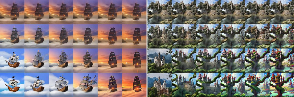
Figure 5 shows additional results using DeepFloyd IF, similar to Figure 4.

图 5 给出与图 4 类似的 DeepFloyd IF 补充结果。

Interpolation between CFG and our method Increasing CFG weight Increasing guidance weight for our method “A pirate ship sailing through clouds instead of the ocean” Increasing CFG weight Increasing guidance weight for our method “A fairytale castle floating in the sky, tethered by ancient vines”

Increasing CFG weight

Increasing guidance weight for our method

Increasing CFG weight

Increasing guidance weight for our method

Figure 5: Additional results for DeepFloyd IF [50]. The rows correspond to guidance weights $w\in\{1,2,3,4\}$. CFG and our method (XL-sized model guided by M-sized one) on the leftmost and rightmost column, respectively. The middle columns correspond to blending between the two.

CFG 与我们方法之间的插值　　增大 CFG 权重　　增大我们方法的引导权重

“A pirate ship sailing through clouds instead of the ocean”

“A fairytale castle floating in the sky, tethered by ancient vines”

图 5：DeepFloyd IF [50] 的补充结果。行对应引导权重 $w\in\{1,2,3,4\}$。CFG 与我们的方法（XL 由 M 引导）分别在最左与最右列；中间列为二者混合。

Figure 6 plots FID and FDDINOv2 as functions of guidance weight, showing that autoguidance is less sensitive to the exact choice of $w$ than CFG. Figure 7 shows example grids that demonstrate that autoguidance retains much higher variation than CFG. Figure 8 provides additional visualizations from our toy example, showing how the implied densities evolve during inference with CFG and autoguidance.

图 6 把 FID 与 FDDINOv2 画成引导权重的函数，显示自引导对 $w$ 的精确选择不如 CFG 敏感。图 7 的示例网格表明自引导保留的多样性远高于 CFG。图 8 为我们玩具例子提供额外可视化，展示推理过程中 CFG 与自引导下隐含密度如何演化。

2.23

1.68

1.34

52.32

46.25

36.67

(a) FID

(a) FID

Ours CFG

Figure 7: Resulting variation for CFG and our method in Tree frog, Minibus, Mushroom classes of ImageNet-512 using EDM2-S (FDDINOv2-optimized). In this image, we have exaggerated the amount of guidance ($w=4$) to make its effect on variation more clearly visible. This causes excessive saturation and other image artifacts, but clearly shows that CFG steers towards canonical templates, while our method preserves much greater variation.

图 7：用 EDM2-S（按 FDDINOv2 优化）在 ImageNet-512 的 Tree frog、Minibus、Mushroom 类别上，CFG 与我们方法所得的结果多样性。本图夸大引导量（$w=4$）以便更清楚看见对多样性的影响。这会造成过度饱和等伪影，但清楚显示 CFG 驶向典型模板，而我们的方法保留大得多的多样性。

$\sigma=0$

(a) $p_{1}(\mathbf{x}|\mathbf{c};\sigma)$

(b) CFG $p_{0}(\mathbf{x};\sigma)$

(c) Autoguidance $p_{0}(\mathbf{x}|\mathbf{c};\sigma)$

(d) CFG ratio $p_{1}/p_{0}$

(e) Autoguidance ratio $p_{1}/p_{0}$

$\sigma=0.5$

$\sigma=0.25$

$\sigma=0.08$

$\sigma=0.03$

$\sigma=0.01$

Figure 8: Progression of implied learned densities during sampling over various $\sigma$ in a setup similar to Figure 2. Contours of the corresponding ground truth distributions are also shown. (a) Main model density $p_{1}(\mathbf{x}|\mathbf{c};\sigma)$. (b) Unconditional guiding model density $p_{0}(\mathbf{x};\sigma)$ in CFG. (c) Conditional guiding model density $p_{0}(\mathbf{x}|\mathbf{c};\sigma)$ in autoguidance. (d) With CFG, guidance towards higher ratio $p_{1}/p_{0}$ pushes samples towards top right, especially at high $\sigma$ (top rows). (e) With autoguidance, this anomalous effect does not occur and samples cover the entire class $\mathbf{c}$.

图 8：与图 2 类似设定下，采样过程中各 $\sigma$ 处隐含学得密度的进展；同时给出对应真实分布的等高线。(a) 主模型密度 $p_{1}(\mathbf{x}|\mathbf{c};\sigma)$。(b) CFG 中无条件引导模型密度 $p_{0}(\mathbf{x};\sigma)$。(c) 自引导中条件引导模型密度 $p_{0}(\mathbf{x}|\mathbf{c};\sigma)$。(d) CFG 下，朝向更高比值 $p_{1}/p_{0}$ 的引导把样本推向右上，尤其在高 $\sigma$（上行）。(e) 自引导下无此异常效应，样本覆盖整个类别 $\mathbf{c}$。

Appendix B Implementation details

附录 B 实现细节

We performed our main experiments on top of the publicly available EDM2 [24] codebase[^4] using NVIDIA A100 GPUs, Python 3.11.7, PyTorch 2.2.0, CUDA 11.8, and CuDNN 8.9.7. Since our method only involves using a different guiding model during sampling, we were able to perform all measurements using the existing command-line scripts. We only had to modify one line of code in the sampling loop to pass in the class label to the guiding network in addition to the main network. Algorithm 1 demonstrates the steps needed to reproduce one of our results from Table 1; the rest can be reproduced by repeating the same steps with different models and hyperparameters as indicated in the table. For the four cases where a pre-trained model was unavailable, we trained the models ourselves as detailed in Algorithm 2.

主要实验基于公开可用的 EDM2 [24] 代码库[^4]，使用 NVIDIA A100 GPU、Python 3.11.7、PyTorch 2.2.0、CUDA 11.8 与 CuDNN 8.9.7。因方法只涉及采样时换用不同引导模型，所有度量均可用现有命令行脚本完成。我们只需改采样循环中的一行代码，使类别标签同时传给引导网络与主网络。算法 1 演示复现表 1 中某一结果所需步骤；其余结果用表中所示不同模型与超参重复相同步骤即可。对四个无预训练模型的情形，我们按算法 2 自行训练。

B.1 Hyperparameter search

B.1 超参搜索

We optimized the autoguidance parameters for each configuration in Table 1 and Figure  using automated grid search. We performed the search separately for FID and FDDINOv2 across the space of five parameters:

我们对表 1 与图中各配置的自引导参数做自动化网格搜索优化。对 FID 与 FDDINOv2 分别在五维参数空间中搜索：

• • Model capacity: All available model capacities (EDM2-XXS, EDM2-XS, etc.) up to and including the capacity of the main model.
• • Training time: Number of training images in powers of two. We found that the sweet spot was always within the range $\{2^{26},2^{27},2^{28},2^{29}\}$ — there was no need to go for lower or higher values.
• • Guidance weight: All values within $[1.00,3.50]$ at regular intervals of $0.05$.
• • EMA lengths: All values within $[0.010,0.250]$ at regular intervals of $0.005$. We treated the EMA length of the main model and the guiding model as two separate parameters.

• • 模型容量： 所有可用容量（EDM2-XXS、EDM2-XS 等），上限为主模型容量。
• • 训练时间： 训练图像数取二的幂。我们发现甜点始终落在 $\{2^{26},2^{27},2^{28},2^{29}\}$——无需更低或更高。
• • 引导权重： $[1.00,3.50]$ 内以 $0.05$ 为间隔的全部取值。
• • EMA 长度： $[0.010,0.250]$ 内以 $0.005$ 为间隔的全部取值。主模型与引导模型的 EMA 长度作为两个独立参数。

In order to reduce the computational workload, we pruned the search space by considering only a local neighborhood of parameters around the best FID or FDDINOv2 found thus far. Whenever the result improved, we placed a new local grid around the corresponding parameters, resulting in gradual convergence towards the global optimum. Once we reached the optimum, we further re-evaluated the nearby parameter choices two more times to account for the effect of random noise. As such, each result reported in Table 1 and Figure  represents the best of three evaluations. The typical range of random variation is indicated by the shaded regions in Figure .

为降低计算量，我们只在迄今最佳 FID 或 FDDINOv2 附近的局部邻域内剪枝搜索空间。结果一改善，就在对应参数周围放新的局部网格，逐步收敛到全局最优。到达最优后，再对邻近参数选择额外评估两次，以计入随机噪声。因此表 1 与图中每个结果代表三次评估中的最佳。随机波动的典型范围由图中阴影区域标出。

In total, the grid search resulted in roughly 30,000 metric evaluations across all of our configurations. In each metric evaluation, the main cost comes from generating 50,000 random images, which takes around 30–60 minutes using eight A100 GPUs and consumes approximately 2–5 kWh of energy, depending on model size. The overall energy consumption of our entire project was thus in the ballpark of 60–150 MWh.

网格搜索在全部配置上共产生约 3 万次度量评估。每次评估的主要成本是生成 5 万张随机图像：八张 A100 约需 30–60 分钟，能耗约 2–5 kWh，视模型大小而定。整个项目总能耗约在 60–150 MWh 量级。

B.2 DeepFloyd IF experiments

B.2 DeepFloyd IF 实验

In order to apply CFG and autoguidance simultaneously, we extend Equation 3 to cover multiple guiding models as proposed by Liu et al. [31]. In this case, we have three models: the main model $D_{\text{m}}$, an unconditional model $D_{\text{u}}$, and a reduced-capacity conditional model $D_{\text{c}}$. The guided denoising result is then defined as

为同时施加 CFG 与自引导，我们按 Liu 等人 [31] 把式 3 扩展到多个引导模型。此时有三个模型：主模型 $D_{\text{m}}$、无条件模型 $D_{\text{u}}$、以及降容量的条件模型 $D_{\text{c}}$。引导后的去噪结果定义为

$$\displaystyle D_{w}(\mathbf{x};\sigma,\mathbf{c}) \\ \displaystyle\,\coloneqq\,D_{\text{m}}(\mathbf{x};\sigma,\mathbf{c})\,+\!\!\sum_{i\in\{\text{u},\text{c}\}}\!(w_{i}-1)\big(D_{\text{m}}(\mathbf{x};\sigma,\mathbf{c})-D_{i}(\mathbf{x};\sigma,\mathbf{c})\big)\text{,} \tag{6}$$

where $w_{\text{u}}$ and $w_{\text{c}}$ correspond to the guidance weights for CFG and autoguidance, respectively. To interpolate between the two methods, we further define $w_{\text{u}}\coloneqq(1-\alpha)(w-1)+1$ and $w_{\text{c}}\coloneqq\alpha(w-1)+1$, where $w$ indicates the desired total amount of guidance and $\alpha\in[0,1]$ is a linear interpolation factor.

其中 $w_{\text{u}}$、$w_{\text{c}}$ 分别对应 CFG 与自引导的引导权重。为在两方法间插值，进一步定义 $w_{\text{u}}\coloneqq(1-\alpha)(w-1)+1$、$w_{\text{c}}\coloneqq\alpha(w-1)+1$，其中 $w$ 为期望的总引导量，$\alpha\in[0,1]$ 为线性插值因子。

DeepFloyd IF [50] uses a three-stage cascade: a base model followed by two super-resolution stages. We apply our method only to the base model, while the super-resolution stages always use CFG with their default weights (4 and 9). We use their Stochastic DDPM sampler with default settings: 100, 75, 50 steps for the base model and subsequent super-resolution stages, respectively. Dynamic thresholding [45] is used for all stages.

DeepFloyd IF [50] 使用三级级联：基座模型后接两个超分阶段。我们只对基座模型应用本方法；超分阶段始终用默认权重（4 与 9）的 CFG。采样器用其 Stochastic DDPM，默认设置：基座与后续超分阶段分别为 100、75、50 步。各阶段均使用动态阈值 [45]。

1 # Download EDM2 source code.
2 git clone https://github.com/NVlabs/edm2.git
3 cd edm2
4 git checkout 32ecad3
5
6 # Patch the sampler so that class labels are passed in to the guiding network.
7 sed -i ’s/gnet(x, t)/gnet(x, t, labels)/g’ generate_images.py
8
9 # Download the necessary EDM2 models.
10 rclone copy --progress --http-url https://nvlabs-fi-cdn.nvidia.com/edm2
11 :http:raw-snapshots/edm2-img512-s/ raw-snapshots/edm2-img512-s/
12 rclone copy --progress --http-url https://nvlabs-fi-cdn.nvidia.com/edm2
13 :http:raw-snapshots/edm2-img512-xs/ raw-snapshots/edm2-img512-xs/
14
15 # Reconstruct the corresponding post-hoc EMA models.
16 python reconstruct_phema.py --indir=raw-snapshots/edm2-img512-s --outdir=autoguidance/phema
17 --outprefix=img512-s --outkimg=2147483 --outstd=0.070
18 python reconstruct_phema.py --indir=raw-snapshots/edm2-img512-xs --outdir=autoguidance/phema
19 --outprefix=img512-xs --outkimg=134217 --outstd=0.125
20
21 # Generate 50,000 images using 8 GPUs.
22 torchrun --standalone --nproc_per_node=8 generate_images.py --seeds=0-49999 --subdirs
23 --outdir=autoguidance/images/img512-s --net=autoguidance/phema/img512-s-2147483-0.070.pkl
24 --gnet=autoguidance/phema/img512-xs-0134217-0.125.pkl --guidance=2.10
25
26 # Calculate FID.
27 python calculate_metrics.py calc --images=autoguidance/images/img512-s
28 --ref=https://nvlabs-fi-cdn.nvidia.com/edm2/dataset-refs/img512.pkl

Algorithm 1   $/$Reproducing our FID result for the “Autoguidance (XS, $T/16$)” row in Table 1.

算法 1　复现表 1 中「自引导（XS，$T/16$）」行 FID 结果的步骤。

Appendix C Details of the 2D toy example

附录 C 二维玩具例子细节

In this section, we describe the construction of the 2D toy dataset used in the analysis of Section 3, as well as the associated model architecture, training setup, and sampling parameters. The related code is available at https://github.com/NVlabs/edm2

本节描述第 3 节分析所用二维玩具数据集的构造，以及相关模型架构、训练设置与采样参数。相关代码见 https://github.com/NVlabs/edm2

Dataset.

For each of the two classes $\mathbf{c}$, we model the fractal-like data distribution as a mixture of Gaussians $\mathcal{M}_{\mathbf{c}}=\big(\{\phi_{i}\},\{\mathbf{\mu}_{i}\},\{\mathbf{\Sigma}_{i}\}\big)$, where $\phi_{i}$, $\mathbf{\mu}_{i}$, and $\mathbf{\Sigma}_{i}$ represent the weight, mean, and $2{\times}2$ covariance matrix of each component $i$, respectively. This lets us calculate the ground truth scores and probability densities analytically and, consequently, to visualize them without making any additional assumptions. The probability density for a given class is given by

数据集。

对两个类别 $\mathbf{c}$ 中的每一个，我们把分形式数据分布建模为高斯混合 $\mathcal{M}_{\mathbf{c}}=\big(\{\phi_{i}\},\{\mathbf{\mu}_{i}\},\{\mathbf{\Sigma}_{i}\}\big)$，其中 $\phi_{i}$、$\mathbf{\mu}_{i}$、$\mathbf{\Sigma}_{i}$ 分别是各分量 $i$ 的权重、均值与 $2{\times}2$ 协方差。这样可解析计算真实得分与概率密度，从而在可视化时无需额外假设。给定类别的概率密度为

$$\displaystyle p_{\text{data}}(\mathbf{x}|\mathbf{c}) \\ \displaystyle\,=\,\sum_{i\in\mathcal{M}_{\mathbf{c}}}\!\phi_{i}\,\mathcal{N}(\mathbf{x};\mathbf{\mu}_{i},\mathbf{\Sigma}_{i})\text{,}\hskip 8.53581pt\text{where} \\ \displaystyle\mathcal{N}(\mathbf{x};\mathbf{\mu},\mathbf{\Sigma}) \\ \displaystyle\,=\,\frac{1}{\sqrt{(2\pi)^{2}\det(\mathbf{\Sigma})}}\exp\bigg(\!-\frac{1}{2}(\mathbf{x}-\mathbf{\mu})^{\top}\mathbf{\Sigma}^{-1}(\mathbf{x}-\mathbf{\mu})\bigg)\text{.} \tag{7}$$

Applying heat diffusion to $p_{\text{data}}(\mathbf{x}|\mathbf{c})$, we obtain a sequence of increasingly smoothed densities $p(\mathbf{x}|\mathbf{c};\sigma)$ parameterized by noise level $\sigma$:

对 $p_{\text{data}}(\mathbf{x}|\mathbf{c})$ 施加热扩散，得到由噪声水平 $\sigma$ 参数化的一串越来越平滑的密度 $p(\mathbf{x}|\mathbf{c};\sigma)$：

$$\displaystyle p(\mathbf{x}|\mathbf{c};\sigma) \\ \displaystyle\,=\,\sum_{i\in\mathcal{M}_{\mathbf{c}}}\!\phi_{i}\,\mathcal{N}\big(\mathbf{x};\mathbf{\mu}_{i},\mathbf{\Sigma}^{\ast}_{i,\sigma}\big)\text{,}\hskip 8.53581pt\text{where}\hskip 5.69054pt\mathbf{\Sigma}^{\ast}_{i,\sigma}=\,\mathbf{\Sigma}_{i}+\sigma^{2}\mathbf{I}\text{.} \tag{9}$$

The score function of $p(\mathbf{x}|\mathbf{c};\sigma)$ is then given by

$p(\mathbf{x}|\mathbf{c};\sigma)$ 的得分函数于是为

$$\displaystyle\smash{\nabla_{\hskip-0.98329pt\mathbf{x}}\hskip-0.50003pt}\log p(\mathbf{x}|\mathbf{c};\sigma) \\ \displaystyle\,=\,\frac{\sum_{i\in\mathcal{M}_{\mathbf{c}}}\phi_{i}\,\mathcal{N}\big(\mathbf{x};\mathbf{\mu}_{i},\mathbf{\Sigma}^{\ast}_{i,\sigma}\big)\,\big(\mathbf{\Sigma}^{\ast}_{i,\sigma}\big)^{-1}\big(\mathbf{\mu}_{i}-\mathbf{x}\big)}{\sum_{i\in\mathcal{M}_{\mathbf{c}}}\phi_{i}\,\mathcal{N}\big(\mathbf{x};\mathbf{\mu}_{i},\mathbf{\Sigma}^{\ast}_{i,\sigma}\big)}\text{.} \tag{10}$$

1 # Unconditional EDM2-S with ImageNet-512, used as a main model in Table 1.
2 torchrun --nnodes=4 --nproc_per_node=8 train_edm2.py
3 --outdir=autoguidance/train/img512-s-uncond --data=datasets/img512-sd.zip --cond=0
4 --preset=edm2-img512-s --duration=2048Mi
5
6 # Unconditional EDM2-XS with ImageNet-64, used as a guiding model in Table 1.
7 torchrun --nnodes=4 --nproc_per_node=8 train_edm2.py
8 --outdir=autoguidance/train/img64-xs-uncond --data=datasets/img64.zip --cond=0
9 --preset=edm2-img64-s --channels=128 --lr=0.0120 --duration=2048Mi
10
11 # Conditional EDM2-XS with ImageNet-64, used as a guiding model in Table 1.
12 torchrun --nnodes=4 --nproc_per_node=8 train_edm2.py
13 --outdir=autoguidance/train/img64-xs --data=datasets/img64.zip --cond=1
14 --preset=edm2-img64-s --channels=128 --lr=0.0120 --duration=512Mi
15
16 # Conditional EDM2-XXS with ImageNet-512, used as a guiding model in Figure 3b.
17 torchrun --nnodes=4 --nproc_per_node=8 train_edm2.py
18 --outdir=autoguidance/train/img512-xxs --data=datasets/img512-sd.zip --cond=1
19 --preset=edm2-img512-xs --channels=64 --lr=0.0170 --duration=512Mi

Algorithm 2   $/$Training the additional EDM2 models needed in Section 5.

算法 2　训练第 5 节所需额外 EDM2 模型的步骤。

We construct $\mathcal{M}_{\mathbf{c}}$ to represent a thin tree-like structure by starting with one main “branch” and recursively subdividing it into smaller ones. Each branch is represented by 8 anisotropic Gaussian components and the subdivision is performed 6 times, decaying $\phi$ after each subdivision and slightly randomizing the lengths and orientations of the two resulting sub-branches. This yields $127{\times}8=1016$ components per class and $1016{\times}2=2032$ components in total. We define the coordinate system so that the mean and standard deviation of $p_{\text{data}}$, marginalized over $\mathbf{c}$, are equal to $0$ and $\sigma_{\text{data}}=0.5$ along each axis, respectively, matching the recommendations by Karras et al. [23].

我们把 $\mathcal{M}_{\mathbf{c}}$ 构造成细树状结构：从一根主「枝」开始，递归细分为更小枝。每枝由 8 个各向异性高斯分量表示，细分进行 6 次，每次细分后衰减 $\phi$，并略微随机化两根子枝的长度与朝向。每类得到 $127{\times}8=1016$ 个分量，合计 $1016{\times}2=2032$ 个。坐标系定义为：对 $\mathbf{c}$ 边缘化后的 $p_{\text{data}}$ 在各轴上均值与标准差分别为 $0$ 与 $\sigma_{\text{data}}=0.5$，以匹配 Karras 等人 [23] 的建议。

Models.

We implement the denoiser models $D_{0}$ and $D_{1}$ as simple multi-layer perceptrons, utilizing the magnitude-preserving design principles from EDM2 [24]. To be able to visualize the implied probability densities in Figure 2, we design the model interface so that for a given noisy sample, each model outputs a single scalar representing the logarithm of the corresponding unnormalized probability density, as opposed to directly outputting the denoised sample or the score vector. Concretely, let us denote the output of a given model by $G_{\theta}(\mathbf{x};\sigma,\mathbf{c})$. The corresponding normalized probability density is then given by

模型。

去噪模型 $D_{0}$、$D_{1}$ 实现为简单多层感知机，采用 EDM2 [24] 的保模长设计原则。为能在图 2 中可视化隐含概率密度，我们把模型接口设计成：对给定噪声样本，每个模型输出一个标量，表示对应未归一化概率密度的对数，而不是直接输出去噪样本或得分向量。具体地，记给定模型输出为 $G_{\theta}(\mathbf{x};\sigma,\mathbf{c})$。对应归一化概率密度为

$$\displaystyle p_{\theta}(\mathbf{x}|\mathbf{c};\sigma) \\ \displaystyle\,=\,\exp\big(G_{\theta}(\mathbf{x};\sigma,\mathbf{c})\big)\,\Big/\int\exp\big(G_{\theta}(\mathbf{x};\sigma,\mathbf{c})\big)\,\mathrm{d}\mathbf{x}\text{.} \tag{11}$$

By virtue of defining $G_{\theta}$ this way, we can derive the score vector, and by extension, the denoised sample, from $G_{\theta}$ through automatic differentiation:

凭借如此定义 $G_{\theta}$，可通过自动微分从 $G_{\theta}$ 导出得分向量，进而导出去噪样本：

$$\displaystyle\smash{\nabla_{\hskip-0.98329pt\mathbf{x}}\hskip-0.50003pt}\log p_{\theta}(\mathbf{x}|\mathbf{c};\sigma) \\ \displaystyle\,=\,\smash{\nabla_{\hskip-0.98329pt\mathbf{x}}\hskip-0.50003pt}\,G_{\theta}(\mathbf{x};\sigma,\mathbf{c}) \\ \displaystyle D_{\theta}(\mathbf{x};\sigma,\mathbf{c}) \\ \displaystyle\,=\,\mathbf{x}+\sigma^{2}\smash{\nabla_{\hskip-0.98329pt\mathbf{x}}\hskip-0.50003pt}\,G_{\theta}(\mathbf{x};\sigma,\mathbf{c})\text{.} \tag{12}$$

Besides Equation 12, we also tried out the alternative formulations where the model outputs the score vector or the denoised sample directly. The results produced by all these variants were qualitatively more or less identical; we chose to go with the formulation above purely for convenience.

除式 12 外，我们也试过让模型直接输出得分向量或去噪样本的替代形式。各变体结果在定性上大体相同；选上述形式纯粹为了方便。

To connect the above definition of $G_{\theta}$ to the raw network layers, we apply preconditioning using the same general principles as in EDM [23]. Denoting the function represented by the raw network layers as $F_{\theta}$, we define $G_{\theta}$ as

为把上述 $G_{\theta}$ 定义接到原始网络层，我们采用与 EDM [23] 相同的一般预条件化原则。记原始网络层表示的函数为 $F_{\theta}$，定义 $G_{\theta}$ 为

$$\displaystyle G_{\theta}(\mathbf{x};\sigma,\mathbf{c}) \\ \displaystyle\,=\,-\frac{1}{2}\left\lVert\mathbf{x}^{\ast}\right\rVert_{2}^{2}-\frac{g_{\theta}}{\sigma n}\,\sum_{i=1}^{n}F_{\theta,i}\Big(\mathbf{x}^{\ast};\,\frac{1}{4}\log\sigma,\,\mathbf{c}\Big)^{2}\text{,}\hskip 8.53581pt\text{where}\hskip 5.69054pt\mathbf{x}^{\ast}\,=\,\frac{\mathbf{x}}{\sqrt{\sigma^{2}+\sigma_{\text{data}}^{2}}} \tag{14}$$

and the sum is taken over the $n$ output features of $F_{\theta}$. We scale the output of $F_{\theta}$ by a learned scaling factor $g_{\theta}$ that we initialize to zero.

求和遍及 $F_{\theta}$ 的 $n$ 个输出特征。我们用学到的缩放因子 $g_{\theta}$ 缩放 $F_{\theta}$ 的输出，并初始化为零。

The goal of Equation 14 is to satisfy the following three requirements:

式 14 的目标是满足以下三点：

• • The input of $F_{\theta}$ should have zero mean and unit magnitude. This is achieved through the division by $\sqrt{\sigma^{2}+\sigma_{\text{data}}^{2}}$.
• • After initialization, $G_{\theta}$ should represent the best possible first-order approximation of the correct solution. This is achieved through the $-\tfrac{1}{2}\left\lVert\mathbf{x}^{\ast}\right\rVert_{2}^{2}$ term, as well as the fact that $g_{\theta}=0$ after initialization.
• • After training, $\sqrt{g_{\theta}}\cdot F_{\theta}$ should have approximately unit magnitude. This is achieved through the division by $\sigma n$.

• • $F_{\theta}$ 的输入应有零均值与单位模长。这通过除以 $\sqrt{\sigma^{2}+\sigma_{\text{data}}^{2}}$ 实现。
• • 初始化后，$G_{\theta}$ 应表示正确解的最佳一阶近似。这通过 $-\tfrac{1}{2}\left\lVert\mathbf{x}^{\ast}\right\rVert_{2}^{2}$ 项以及初始化后 $g_{\theta}=0$ 实现。
• • 训练后，$\sqrt{g_{\theta}}\cdot F_{\theta}$ 应近似有单位模长。这通过除以 $\sigma n$ 实现。

In practice, we use an MLP with one input layer and four hidden layers, interspersed with SiLU [12] activation functions and implemented using the magnitude-preserving primitives from EDM2 [24]. The input is a 4-dimensional vector $\big[\mathbf{x}^{\ast}_{x};\mathbf{x}^{\ast}_{y};\tfrac{1}{4}\log\sigma;1\big]$ and the output of each hidden layer has $n$ features, where $n=64$ for $D_{1}$ and $32$ for $D_{0}$.

实践中用带一个输入层与四个隐藏层的 MLP，层间插入 SiLU [12] 激活，并用 EDM2 [24] 的保模长原语实现。输入为 4 维向量 $\big[\mathbf{x}^{\ast}_{x};\mathbf{x}^{\ast}_{y};\tfrac{1}{4}\log\sigma;1\big]$，每个隐藏层输出 $n$ 个特征，其中 $D_{1}$ 取 $n=64$，$D_{0}$ 取 $32$。

Training.

Given that we have the exact score function of the ground truth distribution readily available (Equation 9), we train the models using exact score matching [20] for simplicity and increased robustness. We thus define the loss function as

训练。

鉴于真实分布的精确得分函数现成可用（式 9），为简单与更稳健，我们用精确得分匹配 [20] 训练模型。损失函数定义为

$$\displaystyle\mathcal{L}(\theta) \\ \displaystyle\,=\,\mathbb{E}_{\sigma\sim p_{\text{train}},\mathbf{x}\sim p(\mathbf{x};\,\sigma)}\,\sigma^{2}\big\lVert\smash{\nabla_{\hskip-0.98329pt\mathbf{x}}\hskip-0.50003pt}\log p_{\theta}(\mathbf{x};\sigma)-\smash{\nabla_{\hskip-0.98329pt\mathbf{x}}\hskip-0.50003pt}\log p(\mathbf{x};\sigma)\big\rVert^{2}_{2}\text{,} \tag{15}$$

where $\sigma\sim p_{\text{train}}$ is realized as $\log(\sigma)\sim\mathcal{N}(P_{\text{mean}},P_{\text{std}})$ [23]. As an alternative to exact score matching, we also experimented with the more commonly used denoising score matching, but did not observe any noticeable differences in model behavior or training dynamics.

其中 $\sigma\sim p_{\text{train}}$ 实现为 $\log(\sigma)\sim\mathcal{N}(P_{\text{mean}},P_{\text{std}})$ [23]。作为精确得分匹配的替代，我们也试过更常用的去噪得分匹配，但未观察到模型行为或训练动态有明显差异。

We train $D_{1}$ for 4096 iterations using a batch size of 4096 samples, and $D_{0}$ for 512 iterations. We set $P_{\text{mean}}\!=-2.3$ and $P_{\text{std}}\!=1.5$, and use $\alpha_{\text{ref}}/\sqrt{\max(t/t_{\text{ref}},1)}$ learning rate decay schedule with $\alpha_{\text{ref}}\!=0.01$ and $t_{\text{ref}}\!=512$ iterations, along with a power function EMA profile [24] with $\sigma_{\text{rel}}\!=0.010$. Overall, the setup is robust with respect to the hyperparameters; the phenomena illustrated in Figures 1 and 2 remain unchanged across a wide range of parameter choices.

我们训练 $D_{1}$ 共 4096 次迭代、批大小 4096；$D_{0}$ 训练 512 次迭代。设 $P_{\text{mean}}\!=-2.3$、$P_{\text{std}}\!=1.5$，并用 $\alpha_{\text{ref}}/\sqrt{\max(t/t_{\text{ref}},1)}$ 学习率衰减，其中 $\alpha_{\text{ref}}\!=0.01$、$t_{\text{ref}}\!=512$ 次迭代，以及幂函数 EMA 曲线 [24]（$\sigma_{\text{rel}}\!=0.010$）。总体而言，设置对超参稳健；图 1、图 2 所示现象在很宽的参数选择范围内保持不变。

Sampling.

We use the standard EDM sampler [23] with $N=32$ Heun steps ($\text{NFE}=63$), $\sigma_{\text{min}}\!=0.002$, $\sigma_{\text{max}}\!=5$, and $\rho=7$. We chose the values of $N$ and $\sigma_{\text{max}}$ to be much higher than what is actually needed for this dataset in order to avoid potential discretization errors from affecting our conclusions. In Figure 1, we set $w=4$ for CFG and $w=3$ for autoguidance, and multiply the score vectors (Equation 12) by $1.40$ for naive truncation. In Figure 2, we set $w=4$ and $\sigma_{\text{mid}}\!=0.03$.

采样。

我们使用标准 EDM 采样器 [23]：$N=32$ 步 Heun（$\text{NFE}=63$），$\sigma_{\text{min}}\!=0.002$，$\sigma_{\text{max}}\!=5$，$\rho=7$。刻意把 $N$ 与 $\sigma_{\text{max}}$ 取得远高于该数据集实际所需，以免离散化误差影响结论。图 1 中 CFG 取 $w=4$、自引导取 $w=3$，朴素截断把得分向量（式 12）乘以 $1.40$。图 2 中取 $w=4$、$\sigma_{\text{mid}}\!=0.03$。

Appendix D Broader societal impact

附录 D 更广泛的社会影响

Generative modeling, including images and videos, has significant misuse potential. It can trigger negative consequences within the society in several ways. The primary concerns include various types of disinformation, but also the potential to amplify stereotypes and unwanted biases [34]. Our improvements to the sample quality can make the results even more believable, even when used for disinformation. That said, we do not unlock any novel uses of the technology.

生成建模（含图像与视频）有显著滥用潜力，可能以多种方式对社会造成负面影响。主要担忧包括各类虚假信息，以及放大刻板印象与不良偏见 [34]。我们对样本质量的提升可能使结果更可信，即便被用于虚假信息。不过，我们并未解锁该技术的任何全新用途。

Appendix E Licenses

附录 E 许可

• • EDM2 models [24]: Creative Commons BY-NC-SA 4.0 license
• • DeepFloyd IF models [50]: Modified MIT license
• • Stable Diffusion VAE model [42]: CreativeML Open RAIL++-M license
• • InceptionV3 model [52]: Apache 2.0 license
• • DINOv2 model [37]: Apache 2.0 license
• • ImageNet dataset [8]: Custom non-commercial license

• • EDM2 模型 [24]：Creative Commons BY-NC-SA 4.0 许可
• • DeepFloyd IF 模型 [50]：Modified MIT 许可
• • Stable Diffusion VAE 模型 [42]：CreativeML Open RAIL++-M 许可
• • InceptionV3 模型 [52]：Apache 2.0 许可
• • DINOv2 模型 [37]：Apache 2.0 许可
• • ImageNet 数据集 [8]：定制非商业许可