AutoAugment: Learning Augmentation Strategies From Data
AutoAugment: Learning Augmentation Strategies from Data
Google Brain
^{∗} Work performed as a member of the Google Brain Residency Program.
^{†} Equal contribution.
Abstract
摘要
Data augmentation is an effective technique for improving the accuracy of modern image classifiers. However, current data augmentation implementations are manually designed. In this paper, we describe a simple procedure called AutoAugment to automatically search for improved data augmentation policies. In our implementation, we have designed a search space where a policy consists of many sub-policies, one of which is randomly chosen for each image in each mini-batch. A sub-policy consists of two operations, each operation being an image processing function such as translation, rotation, or shearing, and the probabilities and magnitudes with which the functions are applied. We use a search algorithm to find the best policy such that the neural network yields the highest validation accuracy on a target dataset. Our method achieves state-of-the-art accuracy on CIFAR-10, CIFAR-100, SVHN, and ImageNet (without additional data). On ImageNet, we attain a Top-1 accuracy of 83.5% which is 0.4% better than the previous record of 83.1%. On CIFAR-10, we achieve an error rate of 1.5%, which is 0.6% better than the previous state-of-the-art. Augmentation policies we find are transferable between datasets. The policy learned on ImageNet transfers well to achieve significant improvements on other datasets, such as Oxford Flowers, Caltech-101, Oxford-IIT Pets, FGVC Aircraft, and Stanford Cars.
数据增广是提高现代图像分类器精度的有效技术。然而,当前的数据增广实现都是手工设计的。本文描述一种称为 AutoAugment 的简单程序,用来自动搜索更好的数据增广策略。在我们的实现中,搜索空间里的一条策略由许多条子策略组成,每张图像在每个小批量里会随机选用其中一条。每条子策略包含两个操作,每个操作都是平移、旋转或剪切这类图像处理函数,并带有施加该函数的概率和幅度。我们用搜索算法寻找最好的策略,使得神经网络在目标数据集上达到最高的验证精度。本方法在 CIFAR-10、CIFAR-100、SVHN 和 ImageNet(不使用额外数据)上达到了当时最高的精度。在 ImageNet 上,我们得到 83.5% 的 Top-1 精度,比此前 83.1% 的纪录高出 0.4%。在 CIFAR-10 上,错误率为 1.5%,比此前最好结果低 0.6%。我们找到的增广策略可以在数据集之间迁移。在 ImageNet 上学到的策略迁移到牛津花、Caltech-101、牛津宠物(Oxford-IIT Pets)、FGVC 飞行器和斯坦福汽车等数据集上,也能带来显著改善。
1. Introduction
1. 引言
Deep neural nets are powerful machine learning systems that tend to work well when trained on massive amounts of data. Data augmentation is an effective technique to increase both the amount and diversity of data by randomly “augmenting” it [3, 54, 29]; in the image domain, common augmentations include translating the image by a few pixels, or flipping the image horizontally. Intuitively, data augmentation is used to teach a model about invariances in the data domain: classifying an object is often insensitive to horizontal flips or translation. Network architectures can also be used to hardcode invariances: convolutional networks bake in translation invariance [16, 32, 25, 29]. However, using data augmentation to incorporate potential invariances can be easier than hardcoding invariances into the model architecture directly.
深度神经网络是强大的机器学习系统,在海量数据上训练时往往表现很好。数据增广通过随机“扩增”数据,是同时增加数据数量和多样性的有效技术 [3, 54, 29];在图像领域,常见增广包括把图像平移几个像素,或做水平翻转。直观上,数据增广是用来让模型学习数据域中的不变性:对物体分类通常对水平翻转或平移并不敏感。网络架构也可以用来把不变性写死:卷积网络就把平移不变性做进了模型里 [16, 32, 25, 29]。不过,用数据增广来纳入潜在的不变性,往往比把这些不变性直接写进模型架构更容易。
| Dataset | GPU hours | Best published results | Our results |
|---|---|---|---|
| CIFAR-10 | 5000 | 2.1 | 1.5 |
| CIFAR-100 | 0 | 12.2 | 10.7 |
| SVHN | 1000 | 1.3 | 1.0 |
| Stanford Cars | 0 | 5.9 | 5.2 |
| ImageNet | 15000 | 3.9 | 3.5 |
Table 1. Error rates (%) from this paper compared to the best results so far on five datasets (Top-5 for ImageNet, Top-1 for the others). Previous best result on Stanford Cars fine-tuned weights originally trained on a larger dataset [66], whereas we use a randomly initialized network. Previous best results on other datasets only include models that were not trained on additional data, for a single evaluation (without ensembling). See Tables 2,3, and 4 for more detailed comparison. GPU hours are estimated for an NVIDIA Tesla P100.
| 数据集 | GPU 小时 | 此前最好发表结果 | 本文结果 |
|---|---|---|---|
| CIFAR-10 | 5000 | 2.1 | 1.5 |
| CIFAR-100 | 0 | 12.2 | 10.7 |
| SVHN | 1000 | 1.3 | 1.0 |
| Stanford Cars | 0 | 5.9 | 5.2 |
| ImageNet | 15000 | 3.9 | 3.5 |
表 1. 本文将五个数据集上的错误率(%)与迄今最好结果相比较(ImageNet 为 Top-5,其余为 Top-1)。斯坦福汽车上此前最好结果微调的是原先在更大数据集上训练过的权重 [66],而我们使用随机初始化的网络。其他数据集上此前最好结果只计入未使用额外数据训练、且为单次评估(不做集成)的模型。更详细的比较见本文表 2、3 和 4。GPU 小时按 NVIDIA Tesla P100 估计。
Yet a large focus of the machine learning and computer vision community has been to engineer better network architectures (e.g., [55, 59, 20, 58, 64, 19, 72, 23, 48]). Less attention has been paid to finding better data augmentation methods that incorporate more invariances. For instance, on ImageNet, the data augmentation approach by [29], introduced in 2012, remains the standard with small changes. Even when augmentation improvements have been found for a particular dataset, they often do not transfer to other datasets as effectively. For example, horizontal flipping of images during training is an effective data augmentation method on CIFAR-10, but not on MNIST, due to the different symmetries present in these datasets. The need for automatically learned data-augmentation has been raised recently as an important unsolved problem [57].
然而,机器学习和计算机视觉社区相当大的精力一直放在设计更好的网络架构上(例如 [55, 59, 20, 58, 64, 19, 72, 23, 48])。对寻找能纳入更多不变性的更好数据增广方法,关注要少得多。例如在 ImageNet 上,[29] 于 2012 年提出的数据增广做法经过少量修改后,至今仍是标准做法。即便为某个数据集找到了更好的增广,它们也往往不能同样有效地迁移到其他数据集。例如,训练时对图像做水平翻转在 CIFAR-10 上是有效的数据增广,但在 MNIST 上并非如此,因为这些数据集中的对称性不同。近来已有工作把自动学习数据增广列为一项重要的未解问题 [57]。
In this paper, we aim to automate the process of finding an effective data augmentation policy for a target dataset. In our implementation (Section 3), each policy expresses several choices and orders of possible augmentation operations, where each operation is an image processing function (e.g., translation, rotation, or color normalization), the probabilities of applying the function, and the magnitudes with which they are applied. We use a search algorithm to find the best choices and orders of these operations such that training a neural network yields the best validation accuracy. In our experiments, we use Reinforcement Learning [71] as the search algorithm, but we believe the results can be further improved if better algorithms are used [48, 39].
本文的目标,是把为给定目标数据集寻找有效数据增广策略的过程自动化。在我们的实现中(第 3 节),每条策略表达了对可能增广操作的若干选择与顺序,其中每个操作都是一种图像处理函数(例如平移、旋转或颜色归一化),并带有施加该函数的概率以及施加时的幅度。我们用搜索算法寻找这些操作的最佳选择与顺序,使得训练神经网络能得到最好的验证精度。实验中我们用强化学习 [71] 作为搜索算法,但我们相信,如果采用更好的算法,结果还可以进一步提高 [48, 39]。
Our extensive experiments show that AutoAugment achieves excellent improvements in two use cases: 1) AutoAugment can be applied directly on the dataset of interest to find the best augmentation policy (AutoAugment-direct) and 2) learned policies can be transferred to new datasets (AutoAugment-transfer). Firstly, for direct application, our method achieves state-of-the-art accuracy on datasets such as CIFAR-10, reduced CIFAR-10, CIFAR-100, SVHN, reduced SVHN, and ImageNet (without additional data). On CIFAR-10, we achieve an error rate of 1.5%, which is 0.6% better than the previous state-of-the-art [48]. On SVHN, we improve the state-of-the-art error rate from 1.3% [12] to 1.0%. On reduced datasets, our method achieves performance comparable to semi-supervised methods without using any unlabeled data. On ImageNet, we achieve a Top-1 accuracy of 83.5% which is 0.4% better than the previous record of 83.1%. Secondly, if direct application is too expensive, transferring an augmentation policy can be a good alternative. For transferring an augmentation policy, we show that policies found on one task can generalize well across different models and datasets. For example, the policy found on ImageNet leads to significant improvements on a variety of FGVC datasets. Even on datasets for which fine-tuning weights pre-trained on ImageNet does not help significantly [26], e.g. Stanford Cars [27] and FGVC Aircraft [38], training with the ImageNet policy reduces test set error by 1.2% and 1.8%, respectively. This result suggests that transferring data augmentation policies offers an alternative method for standard weight transfer learning. A summary of our results is shown in Table 1.
大量实验表明,AutoAugment 在两种使用情形下都能带来出色的改善:1)可以直接在感兴趣的数据集上应用,以寻找最好的增广策略(AutoAugment-direct);2)学到的策略可以迁移到新的数据集(AutoAugment-transfer)。首先,就直接应用而言,本方法在 CIFAR-10、缩小的 CIFAR-10、CIFAR-100、SVHN、缩小的 SVHN 以及 ImageNet(不使用额外数据)等数据集上达到了当时最高精度。在 CIFAR-10 上,错误率为 1.5%,比此前最好结果低 0.6% [48]。在 SVHN 上,我们把当时最好错误率从 1.3% [12] 降到 1.0%。在缩小的数据集上,本方法在不使用任何未标注数据的情况下,达到了与半监督方法相当的表现。在 ImageNet 上,我们得到 83.5% 的 Top-1 精度,比此前 83.1% 的纪录高出 0.4%。其次,如果直接应用代价太高,迁移一条增广策略可以是很好的替代方案。就策略迁移而言,我们表明在一个任务上找到的策略可以很好地泛化到不同模型和数据集。例如,在 ImageNet 上找到的策略,在多种 FGVC 数据集上带来了显著改善。即便在微调 ImageNet 预训练权重帮助并不显著的数据集上 [26],例如斯坦福汽车 [27] 和 FGVC 飞行器 [38],用 ImageNet 策略训练仍分别把测试错误率降低了 1.2% 和 1.8%。这一结果说明,迁移数据增广策略为常规的权重迁移学习提供了一种替代方法。结果摘要见表 1。
2. Related Work
2. 相关工作
Common data augmentation methods for image recognition have been designed manually and the best augmentation strategies are dataset-specific. For example, on MNIST, most top-ranked models use elastic distortions, scale, translation, and rotation [54, 8, 62, 52]. On natural image datasets, such as CIFAR-10 and ImageNet, random cropping, image mirroring and color shifting / whitening are more common [29]. As these methods are designed manually, they require expert knowledge and time. Our approach of learning data augmentation policies from data in principle can be used for any dataset, not just one.
图像识别中常见的数据增广方法都是手工设计的,最好的增广策略往往因数据集而异。例如在 MNIST 上,多数名列前茅的模型使用弹性形变、缩放、平移和旋转 [54, 8, 62, 52]。在 CIFAR-10 和 ImageNet 这类自然图像数据集上,更常见的是随机裁剪、图像镜像以及颜色偏移/白化 [29]。由于这些方法靠手工设计,需要专家知识和时间。我们这种从数据中学习数据增广策略的方法,原则上可用于任意数据集,而不仅限于某一个。
This paper introduces an automated approach to find data augmentation policies from data. Our approach is inspired by recent advances in architecture search, where reinforcement learning and evolution have been used to discover model architectures from data [71, 4, 72, 7, 35, 13, 34, 46, 49, 63, 48, 9]. Although these methods have improved upon human-designed architectures, it has not been possible to beat the 2% error-rate barrier on CIFAR-10 using architecture search alone.
本文提出一种从数据中自动寻找数据增广策略的方法。这一思路受到近来架构搜索进展的启发,那里强化学习与进化已被用来从数据中发现模型架构 [71, 4, 72, 7, 35, 13, 34, 46, 49, 63, 48, 9]。尽管这些方法已经改进了人工设计的架构,但仅靠架构搜索仍未能突破 CIFAR-10 上 2% 错误率的壁垒。
Previous attempts at learned data augmentations include Smart Augmentation, which proposed a network that automatically generates augmented data by merging two or more samples from the same class [33]. Tran et al. used a Bayesian approach to generate data based on the distribution learned from the training set [61]. DeVries and Taylor used simple transformations in the learned feature space to augment data [11].
此前学习数据增广的尝试包括 Smart Augmentation,它提出用一个网络通过合并两个或多个同类样本来自动生成增广数据 [33]。Tran 等人使用贝叶斯方法,基于从训练集学到的分布来生成数据 [61]。DeVries 和 Taylor 则在学到的特征空间中用简单变换来增广数据 [11]。
Generative adversarial networks have also been used for the purpose of generating additional data (e.g., [45, 41, 70, 2, 56]). The key difference between our method and generative models is that our method generates symbolic transformation operations, whereas generative models, such as GANs, generate the augmented data directly. An exception is work by Ratner et al., who used GANs to generate sequences that describe data augmentation strategies [47].
生成对抗网络也被用来生成额外数据(例如 [45, 41, 70, 2, 56])。我们的方法与生成模型的关键区别在于:我们生成的是符号化的变换操作,而 GAN 这类生成模型直接生成增广后的数据。一个例外是 Ratner 等人的工作,他们用 GAN 来生成描述数据增广策略的序列 [47]。
3. AutoAugment: Searching for best Augmentation policies Directly on the Dataset of Interest
3. AutoAugment:直接在目标数据集上搜索最佳增广策略
We formulate the problem of finding the best augmentation policy as a discrete search problem (see Figure 1). Our method consists of two components: A search algorithm and a search space. At a high level, the search algorithm (implemented as a controller RNN) samples a data augmentation policy S, which has information about what image processing operation to use, the probability of using the operation in each batch, and the magnitude of the operation. Key to our method is the fact that the policy S will be used to train a neural network with a fixed architecture, whose validation accuracy R will be sent back to update the controller. Since R is not differentiable, the controller will be updated by policy gradient methods. In the following section we will describe the two components in detail.
我们把寻找最佳增广策略的问题表述为一个离散搜索问题(见图 1)。本方法由两个部分组成:搜索算法和搜索空间。在较高层面上,搜索算法(实现为一个控制器 RNN)采样一条数据增广策略 ,其中包含使用哪种图像处理操作、在每个批量中使用该操作的概率,以及该操作的幅度。本方法的关键在于:策略 将被用来训练一个架构固定的神经网络,其验证精度 会送回以更新控制器。由于 不可微,控制器将用策略梯度方法来更新。下一节我们将详细描述这两个部分。
Search space details: In our search space, a policy consists of 5 sub-policies with each sub-policy consisting of two image operations to be applied in sequence. Additionally, each operation is also associated with two hyperparameters: 1) the probability of applying the operation, and 2) the magnitude of the operation. Figure 2 shows an example of a policy with 5-sub-policies in our search space. The first sub-policy specifies a sequential application of ShearX followed by Invert. The probability of applying ShearX is 0.9, and when applied, has a magnitude of 7 out of 10. We then apply Invert with probability of 0.8. The Invert operation does not use the magnitude information. We emphasize that these operations are applied in the specified order.
搜索空间细节:在我们的搜索空间中,一条策略由 5 条子策略组成,每条子策略包含两个依次施加的图像操作。此外,每个操作还带有两个超参数:1)施加该操作的概率;2)该操作的幅度。图 2 给出了我们搜索空间中一条含 5 条子策略的策略示例。第一条子策略指定先施加 ShearX,再施加 Invert。施加 ShearX 的概率为 0.9,一旦施加,幅度为 10 档中的 7。随后以 0.8 的概率施加 Invert。Invert 操作不使用幅度信息。我们强调,这些操作按指定顺序施加。
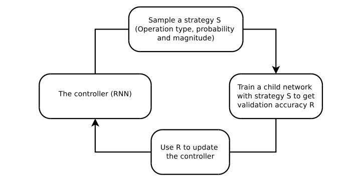
Figure 1. Overview of our framework of using a search method (e.g., Reinforcement Learning) to search for better data augmentation policies. A controller RNN predicts an augmentation policy from the search space. A child network with a fixed architecture is trained to convergence achieving accuracy R. The reward R will be used with the policy gradient method to update the controller so that it can generate better policies over time.
图 1|用某种搜索方法(例如强化学习)搜索更好数据增广策略的框架概览。控制器 RNN 从搜索空间中预测一条增广策略。一个架构固定的子网络被训练到收敛,得到精度 。奖励 将与策略梯度方法一起用来更新控制器,使其随着时间生成更好的策略。
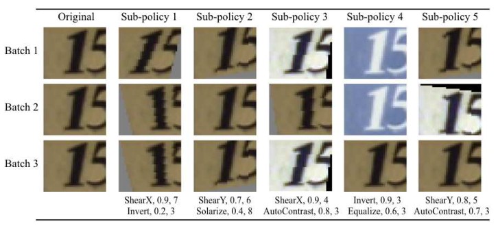
Figure 2. One of the policies found on SVHN, and how it can be used to generate augmented data given an original image used to train a neural network. The policy has 5 sub-policies. For every image in a mini-batch, we choose a sub-policy uniformly at random to generate a transformed image to train the neural network. Each sub-policy consists of 2 operations, each operation is associated with two numerical values: the probability of calling the operation, and the magnitude of the operation. There is a probability of calling an operation, so the operation may not be applied in that mini-batch. However, if applied, it is applied with the fixed magnitude. We highlight the stochasticity in applying the sub-policies by showing how one image can be transformed differently in different mini-batches, even with the same sub-policy. As explained in the text, on SVHN, geometric transformations are picked more often by AutoAugment. It can be seen why Invert is a commonly selected operation on SVHN, since the numbers in the image are invariant to that transformation.
图 2|在 SVHN 上找到的一条策略,以及如何用它在给定用于训练神经网络的原始图像上生成增广数据。该策略有 5 条子策略。对小批量中的每张图像,我们均匀随机选择一条子策略,生成变换后的图像来训练网络。每条子策略包含 2 个操作,每个操作带有两个数值:调用该操作的概率,以及该操作的幅度。由于存在调用概率,该操作在那个小批量中可能并不被施加;但一旦施加,就使用固定的幅度。我们通过展示同一张图像即使使用同一条子策略,在不同小批量中也可以被变换成不同样子,来突出施加子策略时的随机性。如正文所述,在 SVHN 上 AutoAugment 更常选择几何变换。也可以看出 Invert 为何在 SVHN 上常被选中:因为图像中的数字对该变换是不变的。
The operations we used in our experiments are from PIL, a popular Python image library.^{1} For generality, we considered all functions in PIL that accept an image as input and output an image. We additionally used two other promising augmentation techniques: Cutout [12] and SamplePairing [24]. The operations we searched over are ShearX/Y, TranslateX/Y, Rotate, AutoContrast, Invert, Equalize, Solarize, Posterize, Contrast, Color, Brightness, Sharpness, Cutout [12], Sample Pairing [24].^{2} In total, we have 16 operations in our search space. Each operation also comes with a default range of magnitudes, which will be described in more detail in Section 4. We discretize the range of magnitudes into 10 values (uniform spacing) so that we can use a discrete search algorithm to find them. Similarly, we also discretize the probability of applying that operation into 11 values (uniform spacing). Finding each sub-policy becomes a search problem in a space of (16×10×11)^{2} possibilities. Our goal, however, is to find 5 such sub-policies concurrently in order to increase diversity. The search space with 5 sub-policies then has roughly (16×10×11)^{10} ≈ 2.9×10^{32} possibilities.
我们实验中使用的操作来自流行的 Python 图像库 PIL。^{1} 为了具有一般性,我们考虑了 PIL 中所有以图像为输入并以图像为输出的函数。此外还使用了另外两种有前景的增广技术:Cutout [12] 和 SamplePairing [24]。我们搜索的操作是 ShearX/Y、TranslateX/Y、Rotate、AutoContrast、Invert、Equalize、Solarize、Posterize、Contrast、Color、Brightness、Sharpness、Cutout [12]、Sample Pairing [24]。^{2} 搜索空间中一共有 16 种操作。每种操作还带有默认的幅度范围,将在第 4 节中更详细说明。我们把幅度范围离散成 10 个值(均匀间隔),以便用离散搜索算法来寻找。类似地,我们也把施加该操作的概率离散成 11 个值(均匀间隔)。于是,寻找每条子策略变成了在 种可能中的搜索问题。不过,我们的目标是同时找到 5 条这样的子策略,以增加多样性。带有 5 条子策略的搜索空间大约有 种可能。
^{2} Details about these operations are listed in Table 1 in the Appendix.
The 16 operations we used and their default range of values are shown in Table 1 in the Appendix. Notice that there is no explicit “Identity” operation in our search space; this operation is implicit, and can be achieved by calling an operation with probability set to be 0.
我们使用的 16 种操作及其默认取值范围列在附录的表 1 中。注意,我们的搜索空间中没有显式的“恒等”操作;这一操作是隐含的,可以通过把某个操作的概率设为 0 来实现。
Search algorithm details: The search algorithm that we used in our experiment uses Reinforcement Learning, inspired by [71, 4, 72, 5]. The search algorithm has two components: a controller, which is a recurrent neural network, and the training algorithm, which is the Proximal Policy Optimization algorithm [53]. At each step, the controller predicts a decision produced by a softmax; the prediction is then fed into the next step as an embedding. In total the controller has 30 softmax predictions in order to predict 5 sub-policies, each with 2 operations, and each operation requiring an operation type, magnitude and probability.
搜索算法细节:我们实验中使用的搜索算法采用强化学习,其思路受到 [71, 4, 72, 5] 的启发。该搜索算法有两个部分:一个控制器,它是循环神经网络;以及训练算法,即近端策略优化算法 [53]。在每一步,控制器通过一个 softmax 预测一个决策;该预测再作为嵌入送入下一步。控制器一共有 30 个 softmax 预测,用来预测 5 条子策略,每条含 2 个操作,每个操作需要操作类型、幅度和概率。
The training of controller RNN: The controller is trained with a reward signal, which is how good the policy is in improving the generalization of a “child model” (a neural network trained as part of the search process). In our experiments, we set aside a validation set to measure the generalization of a child model. A child model is trained with augmented data generated by applying the 5 sub-policies on the training set (that does not contain the validation set). For each example in the mini-batch, one of the 5 sub-policies is chosen randomly to augment the image. The child model is then evaluated on the validation set to measure the accuracy, which is used as the reward signal to train the recurrent network controller. On each dataset, the controller samples about 15,000 policies.
控制器 RNN 的训练:控制器用一个奖励信号来训练,即该策略在改善“子模型”(作为搜索过程一部分而训练的神经网络)泛化方面有多好。在我们的实验中,会留出一份验证集来衡量子模型的泛化。子模型用把 5 条子策略施加在训练集(不含验证集)上所生成的增广数据来训练。对小批量中的每个样本,随机选择 5 条子策略之一来增广该图像。随后在验证集上评估子模型以得到精度,并以此作为奖励信号来训练循环网络控制器。在每个数据集上,控制器大约采样 15,000 条策略。
Architecture of controller RNN and training hyperparameters: We follow the training procedure and hyperparameters from [72] for training the controller. More concretely, the controller RNN is a one-layer LSTM [21] with 100 hidden units at each layer and 2 × 5B softmax predictions for the two convolutional cells (where B is typically 5) associated with each architecture decision. Each of the 10B predictions of the controller RNN is associated with a probability. The joint probability of a child network is the product of all probabilities at these 10B softmaxes. This joint probability is used to compute the gradient for the controller RNN. The gradient is scaled by the validation accuracy of the child network to update the controller RNN such that the controller assigns low probabilities for bad child networks and high probabilities for good child networks. Similar to [72], we employ Proximal Policy Optimization (PPO) [53] with learning rate 0.00035. To encourage exploration we also use an entropy penalty with a weight of 0.00001. In our implementation, the baseline function is an exponential moving average of previous rewards with a weight of 0.95. The weights of the controller are initialized uniformly between -0.1 and 0.1. We choose to train the controller using PPO out of convenience, although prior work had shown that other methods (e.g. augmented random search and evolutionary strategies) can perform as well or even slightly better [30].
控制器 RNN 的架构与训练超参数:我们沿用 [72] 中的训练程序和超参数来训练控制器。更具体地说,控制器 RNN 是一层 LSTM [21],每层有 100 个隐单元,并且对与每个架构决策相关的两个卷积细胞有 个 softmax 预测(其中 通常为 5)。控制器 RNN 的这 个预测每个都对应一个概率。子网络的联合概率是这 个 softmax 上所有概率的乘积。这一联合概率被用来计算控制器 RNN 的梯度。该梯度再按子网络的验证精度缩放,以更新控制器 RNN,使控制器对差的子网络赋予低概率、对好的子网络赋予高概率。与 [72] 类似,我们使用近端策略优化(PPO)[53],学习率为 0.00035。为了鼓励探索,我们还使用权重为 0.00001 的熵惩罚。在我们的实现中,基线函数是此前奖励的指数移动平均,权重为 0.95。控制器的权重在 -0.1 到 0.1 之间均匀初始化。我们选择用 PPO 训练控制器是出于方便,尽管已有工作表明其他方法(例如增强随机搜索和进化策略)可以做得同样好,甚至略好 [30]。
At the end of the search, we concatenate the sub-policies from the best 5 policies into a single policy (with 25 sub-policies). This final policy with 25 sub-policies is used to train the models for each dataset.
搜索结束时,我们把最好的 5 条策略中的子策略拼接成一条策略(共 25 条子策略)。这条含 25 条子策略的最终策略,被用来训练各个数据集上的模型。
The above search algorithm is one of many possible search algorithms we can use to find the best policies. It might be possible to use a different discrete search algorithm such as genetic programming [48] or even random search [6] to improve the results in this paper.
上述搜索算法只是我们可以用来寻找最佳策略的多种可能搜索算法之一。或许也可以使用不同的离散搜索算法,例如遗传规划 [48],甚至随机搜索 [6],来改进本文的结果。
4. Experiments and Results
4. 实验与结果
Summary of Experiments. In this section, we empirically investigate the performance of AutoAugment in two use cases: AutoAugment-direct and AutoAugment-transfer. First, we will benchmark AutoAugment with direct search for best augmentation policies on highly competitive datasets: CIFAR-10 [28], CIFAR-100 [28], SVHN [42] (Section 4.1), and ImageNet [10] (Section 4.2) datasets. Our results show that a direct application of AutoAugment improves significantly the baseline models and produces state-of-the-art accuracies on these challenging datasets. Next, we will study the transferability of augmentation policies between datasets. More concretely, we will transfer the best augmentation policies found on ImageNet to fine-grained classification datasets such as Oxford 102 Flowers, Caltech-101, Oxford-IIIT Pets, FGVC Aircraft, Stanford Cars (Section 4.3). Our results also show that augmentation policies are surprisingly transferable and yield significant improvements on strong baseline models on these datasets. Finally, in Section 5, we will compare AutoAugment against other automated data augmentation methods and show that AutoAugment is significantly better.
实验摘要。本节从经验上考察 AutoAugment 在两种使用情形下的表现:AutoAugment-direct 和 AutoAugment-transfer。首先,我们将在竞争性很强的数据集上,用直接搜索最佳增广策略的方式对 AutoAugment 做基准测试:CIFAR-10 [28]、CIFAR-100 [28]、SVHN [42](第 4.1 节)以及 ImageNet [10](第 4.2 节)。结果表明,直接应用 AutoAugment 显著改善了基线模型,并在这些有挑战性的数据集上达到了当时最高精度。接下来,我们将研究增广策略在数据集之间的可迁移性。更具体地说,我们会把在 ImageNet 上找到的最佳增广策略迁移到牛津 102 花、Caltech-101、牛津宠物(Oxford-IIIT Pets)、FGVC 飞行器、斯坦福汽车等细粒度分类数据集上(第 4.3 节)。结果也表明,增广策略出人意料地可迁移,并在这些数据集上的强基线模型中带来显著改善。最后,在第 5 节中,我们将把 AutoAugment 与其他自动化数据增广方法相比较,并表明 AutoAugment 明显更好。
4.1. CIFAR-10, CIFAR-100, SVHN Results
4.1. CIFAR-10、CIFAR-100、SVHN 结果
Although CIFAR-10 has 50,000 training examples, we perform the search for the best policies on a smaller dataset we call “reduced CIFAR-10”, which consists of 4,000 randomly chosen examples, to save time for training child models during the augmentation search process (We find that the resulting policies do not seem to be sensitive to this number). We find that for a fixed amount of training time, it is more useful to allow child models to train for more epochs rather than train for fewer epochs with more training data. For the child model architecture we use small Wide-ResNet-40-2 (40 layers - widening factor of 2) model [67], and train for 120 epochs. The use of a small Wide-ResNet is for computational efficiency as each child model is trained from scratch to compute the gradient update for the controller. We use a weight decay of 10^{-4}, learning rate of 0.01, and a cosine learning decay with one annealing cycle [36].
虽然 CIFAR-10 有 50,000 个训练样本,但为了节省增广搜索过程中训练子模型的时间,我们在一个称为“缩小的 CIFAR-10”的更小数据集上搜索最佳策略,它由随机选取的 4,000 个样本组成(我们发现,得到的策略对这个数目似乎并不敏感)。我们还发现,在固定的训练时间下,让子模型训练更多轮次,比用更多训练数据但训练更少轮次更有用。子模型架构我们使用较小的 Wide-ResNet-40-2(40 层,加宽因子为 2)模型 [67],并训练 120 个轮次。使用较小的 Wide-ResNet 是为了计算效率,因为每个子模型都要从头训练,以便计算控制器的梯度更新。我们使用 的权重衰减、0.01 的学习率,以及带一个退火周期的余弦学习率衰减 [36]。
The policies found during the search on reduced CIFAR-10 are later used to train final models on CIFAR-10, reduced CIFAR-10, and CIFAR-100. As mentioned above, we concatenate sub-policies from the best 5 policies to form a single policy with 25 sub-policies, which is used for all of AutoAugment experiments on the CIFAR datasets.
在缩小的 CIFAR-10 上搜索得到的策略,随后被用来在 CIFAR-10、缩小的 CIFAR-10 以及 CIFAR-100 上训练最终模型。如上所述,我们把最好的 5 条策略中的子策略拼接成一条含 25 条子策略的策略,并用于 CIFAR 数据集上的全部 AutoAugment 实验。
The baseline pre-processing follows the convention for state-of-the-art CIFAR-10 models: standardizing the data, using horizontal flips with 50% probability, zero-padding and random crops, and finally Cutout with 16x16 pixels [17, 65, 48, 72]. The AutoAugment policy is applied in addition to the standard baseline pre-processing: on one image, we first apply the baseline augmentation provided by the existing baseline methods, then apply the AutoAugment policy, then apply Cutout. We did not optimize the Cutout region size, and use the suggested value of 16 pixels [12]. Note that since Cutout is an operation in the search space, Cutout may be used twice on the same image: the first time with learned region size, and the second time with fixed region size. In practice, as the probability of the Cutout operation in the first application is small, Cutout is often used once on a given image.
基线预处理遵循当时最好的 CIFAR-10 模型的惯例:对数据做标准化,以 50% 的概率做水平翻转,零填充和随机裁剪,最后使用 16×16 像素的 Cutout [17, 65, 48, 72]。AutoAugment 策略是在标准基线预处理之外再施加的:对一张图像,我们先施加已有基线方法提供的基线增广,再施加 AutoAugment 策略,然后施加 Cutout。我们没有优化 Cutout 区域大小,而是使用建议的 16 像素 [12]。需要注意的是,由于 Cutout 也是搜索空间中的一种操作,同一张图像上 Cutout 可能被使用两次:第一次使用学到的区域大小,第二次使用固定的区域大小。在实践中,由于第一次施加时 Cutout 操作的概率较小,一张给定图像上 Cutout 往往只被使用一次。
On CIFAR-10, AutoAugment picks mostly color-based transformations. For example, the most commonly picked transformations on CIFAR-10 are Equalize, AutoContrast, Color, and Brightness (refer to Table 1 in the Appendix for their descriptions). Geometric transformations like ShearX and ShearY are rarely found in good policies. Furthermore, the transformation Invert is almost never applied in a successful policy. The policy found on CIFAR-10 is included in the Appendix. Below, we describe our results on the CIFAR datasets using the policy found on reduced CIFAR-10. All of the reported results are averaged over 5 runs.
在 CIFAR-10 上,AutoAugment 大多选择基于颜色的变换。例如,在 CIFAR-10 上最常被选中的变换是 Equalize、AutoContrast、Color 和 Brightness(其说明见附录表 1)。ShearX 和 ShearY 这类几何变换很少出现在好的策略中。此外,Invert 变换几乎从不被用在成功的策略里。在 CIFAR-10 上找到的策略收录在附录中。下面,我们描述用在缩小的 CIFAR-10 上找到的策略,在 CIFAR 数据集上得到的结果。所报告的结果均对 5 次运行取平均。
CIFAR-10 Results. In Table 2, we show the test set accuracy on different neural network architectures. We implement the Wide-ResNet-28-10 [67], Shake-Shake [17] and ShakeDrop [65] models in TensorFlow[1], and find the weight decay and learning rate hyperparameters that give the best validation set accuracy for regular training with baseline augmentation. Other hyperparameters are the same as reported in the papers introducing the models [67, 17, 65], with the exception of using a cosine learning decay for the Wide-ResNet-28-10. We then use the same model and hyperparameters to evaluate the test set accuracy of AutoAugment. For AmoebaNets, we use the same hyperparameters that were used in [48] for both baseline augmentation and AutoAugment. As can be seen from the table, we achieve an error rate of 1.5% with the Shake-Drop [65] model, which is 0.6% better than the state-of-the-art [48]. Notice that this gain is much larger than the previous gains obtained by AmoebaNet-B against ShakeDrop (+0.2%), and by ShakeDrop against Shake-Shake (+0.2%). Ref. [68] reports an improvement of 1.1% for a Wide-ResNet-28-10 model trained on CIFAR-10.
CIFAR-10 结果。在表 2 中,我们给出不同神经网络架构上的测试集精度。我们在 TensorFlow[1] 中实现了 Wide-ResNet-28-10 [67]、Shake-Shake [17] 和 ShakeDrop [65] 模型,并寻找在使用基线增广的常规训练中给出最佳验证集精度的权重衰减和学习率超参数。其他超参数与引入这些模型的论文中所报告的相同 [67, 17, 65],例外是 Wide-ResNet-28-10 使用了余弦学习率衰减。然后我们用同一模型和超参数评估 AutoAugment 的测试集精度。对 AmoebaNets,基线增广和 AutoAugment 都使用与 [48] 中相同的超参数。从表中可以看到,我们用 ShakeDrop [65] 模型达到了 1.5% 的错误率,比当时最好结果低 0.6% [48]。需要注意的是,这一增益远大于此前 AmoebaNet-B 相对 ShakeDrop 的增益(+0.2%),以及 ShakeDrop 相对 Shake-Shake 的增益(+0.2%)。文献 [68] 报告,在 CIFAR-10 上训练的 Wide-ResNet-28-10 模型有 1.1% 的改善。
We also evaluate our best model trained with AutoAugment on a recently proposed CIFAR-10 test set [50]. Recht et al. [50] report that Shake-Shake (26 2x64d) + Cutout performs best on this new dataset, with an error rate of 7.0% (4.1% higher relative to error rate on the original CIFAR-10 test set). Furthermore, PyramidNet+ShakeDrop achieves an error rate of 7.7% on the new dataset (4.6% higher relative to the original test set). Our best model, Pyramid-Net+ShakeDrop trained with AutoAugment achieves an error rate of 4.4% (2.9% higher than the error rate on the original set). Compared to other models evaluated on this new dataset, our model exhibits a significantly smaller drop in accuracy.
我们还在一套新近提出的 CIFAR-10 测试集上 [50] 评估了用 AutoAugment 训练的最佳模型。Recht 等人 [50] 报告,Shake-Shake (26 2x64d) + Cutout 在这一新数据集上表现最好,错误率为 7.0%(相对原来的 CIFAR-10 测试集错误率高出 4.1%)。此外,PyramidNet+ShakeDrop 在新数据集上的错误率为 7.7%(相对原测试集高出 4.6%)。我们最好的模型,即用 AutoAugment 训练的 PyramidNet+ShakeDrop,错误率为 4.4%(比在原测试集上的错误率高 2.9%)。与在这一新数据集上评估的其他模型相比,我们的模型精度下降明显更小。
CIFAR-100 Results. We also train models on CIFAR-100 with the same AutoAugment policy found on reduced-CIFAR-10; results are shown in Table 2. Again, we achieve the state-of-art result on this dataset, beating the previous record of 12.19% error rate by ShakeDrop regularization [65].
CIFAR-100 结果。我们还用在缩小的 CIFAR-10 上找到的同一条 AutoAugment 策略,在 CIFAR-100 上训练模型;结果见表 2。我们再次在该数据集上达到了当时最好的结果,超过了 ShakeDrop 正则化此前 12.19% 错误率的纪录 [65]。
Finally, we apply the same AutoAugment policy to train models on reduced CIFAR-10 (the same 4,000 example training set that we use to find the best policy). Similar to the experimental convention used by the semi-supervised learning community [60, 40, 51, 31, 44] we train on 4,000 labeled samples. But we do not use the 46,000 unlabeled samples during training. Our results shown in Table 2. We note that the improvement in accuracy due to AutoAugment is more significant on the reduced dataset compared to the full dataset. As the size of the training set grows, we expect that the effect of data-augmentation will be reduced. However, in the next sections we show that even for larger datasets like SVHN and ImageNet, AutoAugment can still lead to improvements in generalization accuracy.
最后,我们把同一条 AutoAugment 策略用于在缩小的 CIFAR-10 上训练模型(也就是用来寻找最佳策略的那同一份 4,000 个样本的训练集)。与半监督学习社区的实验惯例类似 [60, 40, 51, 31, 44],我们在 4,000 个带标签样本上训练,但训练中不使用那 46,000 个未标注样本。结果见表 2。我们注意到,与完整数据集相比,AutoAugment 在缩小数据集上带来的精度改善更为显著。随着训练集变大,我们预期数据增广的作用会减弱。不过,在接下来的几节中我们将表明,即便对 SVHN 和 ImageNet 这样更大的数据集,AutoAugment 仍然能够改善泛化精度。
SVHN Results We experimented with the SVHN dataset [42], which has 73,257 training examples (also called “core training set”), and 531,131 additional training examples. The test set has 26,032 examples. To save time during the search, we created a reduced SVHN dataset of 1,000 examples sampled randomly from the core training set. We use AutoAugment to find the best policies. The model architecture and training procedure of the child models are identical to the above experiments with CIFAR-10.
SVHN 结果。我们在 SVHN 数据集 [42] 上做了实验,该数据集有 73,257 个训练样本(也称为“核心训练集”),以及 531,131 个额外训练样本。测试集有 26,032 个样本。为了节省搜索时间,我们从核心训练集中随机抽样,构造了一个含 1,000 个样本的缩小 SVHN 数据集。我们用 AutoAugment 寻找最佳策略。子模型的架构和训练程序与上面 CIFAR-10 的实验相同。
The policies picked on SVHN are different than the transformations picked on CIFAR-10. For example, the most commonly picked transformations on SVHN are Invert, Equalize, ShearX/Y, and Rotate. As mentioned above, the transformation Invert is almost never used on CIFAR-10, yet it is very common in successful SVHN policies. Intuitively, this makes sense since the specific color of numbers is not as important as the relative color of the number and its background. Furthermore, geometric transformations ShearX/Y are two of the most popular transformations on SVHN. This also can be understood by general properties of images in SVHN: house numbers are often naturally sheared and skewed in the dataset, so it is helpful to learn the invariance to such transformations via data augmentation. Five successful sub-policies are visualized on SVHN examples in Figure 2.
在 SVHN 上选出的策略,与在 CIFAR-10 上选出的变换不同。例如,SVHN 上最常被选中的变换是 Invert、Equalize、ShearX/Y 和 Rotate。如上所述,Invert 变换在 CIFAR-10 上几乎从不用到,却在成功的 SVHN 策略中非常常见。直观上这说得通,因为数字的具体颜色不如数字与其背景的相对颜色来得重要。此外,几何变换 ShearX/Y 是 SVHN 上最受欢迎的两种变换。这也可用 SVHN 中图像的一般性质来理解:数据集里的门牌号常常天然带有剪切和歪斜,因此通过数据增广来学习对这些变换的不变性是有帮助的。图 2 在 SVHN 样本上可视化了五条成功的子策略。
After the end of the search, we concatenate the 5 best policies and apply them to train architectures that already perform well on SVHN using standard augmentation policies. For full training, we follow the common procedure mentioned in the Wide-ResNet paper [67] of using the core training set and the extra data. The validation set is constructed by setting aside the last 7325 samples of the training set. We tune the weight decay and learning rate on the validation set performance. Other hyperparameters and training details are identical to the those in the papers introducing the models [67, 17]. One exception is that we trained the Shake-Shake model only for 160 epochs (as opposed to 1,800), due to the large size of the full SVHN dataset. Baseline pre-processing involves standardizing the data and applying Cutout with a region size of 20x20 pixels, following the procedure outlined in [12]. AutoAugment results combine the baseline pre-processing with the policy learned on SVHN. One exception is that we do not use Cutout on reduced SVHN as it lowers the accuracy significantly. The summary of the results in this experiment are shown in Table 2. As can be seen from the table, we achieve state-of-the-art accuracy using both models.
搜索结束后,我们把最好的 5 条策略拼接起来,用来训练在标准增广策略下已经在 SVHN 上表现良好的架构。完整训练时,我们遵循 Wide-ResNet 论文 [67] 中提到的常用做法,同时使用核心训练集和额外数据。验证集由训练集最后 7,325 个样本留出构成。我们根据验证集表现来调节权重衰减和学习率。其他超参数和训练细节与引入这些模型的论文相同 [67, 17]。一个例外是,由于完整 SVHN 数据集很大,Shake-Shake 模型我们只训练了 160 个轮次(而不是 1,800 个)。基线预处理包括对数据做标准化,并按照 [12] 中的程序施加区域大小为 20×20 像素的 Cutout。AutoAugment 的结果是把基线预处理与在 SVHN 上学到的策略结合起来。一个例外是,我们在缩小的 SVHN 上不使用 Cutout,因为它会显著降低精度。本实验的结果摘要见表 2。从表中可以看到,两种模型我们都达到了当时最高精度。
| Dataset | Model | Baseline | Cutout [12] | AutoAugment |
|---|---|---|---|---|
| CIFAR-10 | Wide-ResNet-28-10 [67] | 3.9 | 3.1 | 2.6±0.1 |
| Shake-Shake (26 2x32d) [17] | 3.6 | 3.0 | 2.5±0.1 | |
| Shake-Shake (26 2x96d) [17] | 2.9 | 2.6 | 2.0±0.1 | |
| Shake-Shake (26 2x112d) [17] | 2.8 | 2.6 | 1.9±0.1 | |
| AmoebaNet-B (6,128) [48] | 3.0 | 2.1 | 1.8±0.1 | |
| PyramidNet+ShakeDrop [65] | 2.7 | 2.3 | 1.5 ± 0.1 | |
| Reduced CIFAR-10 | Wide-ResNet-28-10 [67] | 18.8 | 16.5 | 14.1±0.3 |
| Shake-Shake (26 2x96d) [17] | 17.1 | 13.4 | 10.0 ± 0.2 | |
| CIFAR-100 | Wide-ResNet-28-10 [67] | 18.8 | 18.4 | 17.1±0.3 |
| Shake-Shake (26 2x96d) [17] | 17.1 | 16.0 | 14.3±0.2 | |
| PyramidNet+ShakeDrop [65] | 14.0 | 12.2 | 10.7 ± 0.2 | |
| SVHN | Wide-ResNet-28-10 [67] | 1.5 | 1.3 | 1.1 |
| Shake-Shake (26 2x96d) [17] | 1.4 | 1.2 | 1.0 | |
| Reduced SVHN | Wide-ResNet-28-10 [67] | 13.2 | 32.5 | 8.2 |
| Shake-Shake (26 2x96d) [17] | 12.3 | 24.2 | 5.9 |
Table 2. Test set error rates (%) on CIFAR-10, CIFAR-100, and SVHN datasets. Lower is better. All the results of the baseline models, and baseline models with Cutout are replicated in our experiments and match the previously reported results [67, 17, 65, 12]. Two exceptions are Shake-Shake (26 2x112d), which has more filters than the biggest model in [17] – 112 vs 96, and Shake-Shake models trained on SVHN, these results were not previously reported. See text for more details.
| 数据集 | 模型 | 基线 | Cutout [12] | AutoAugment |
|---|---|---|---|---|
| CIFAR-10 | Wide-ResNet-28-10 [67] | 3.9 | 3.1 | 2.6±0.1 |
| Shake-Shake (26 2x32d) [17] | 3.6 | 3.0 | 2.5±0.1 | |
| Shake-Shake (26 2x96d) [17] | 2.9 | 2.6 | 2.0±0.1 | |
| Shake-Shake (26 2x112d) [17] | 2.8 | 2.6 | 1.9±0.1 | |
| AmoebaNet-B (6,128) [48] | 3.0 | 2.1 | 1.8±0.1 | |
| PyramidNet+ShakeDrop [65] | 2.7 | 2.3 | 1.5 ± 0.1 | |
| 缩小的 CIFAR-10 | Wide-ResNet-28-10 [67] | 18.8 | 16.5 | 14.1±0.3 |
| Shake-Shake (26 2x96d) [17] | 17.1 | 13.4 | 10.0 ± 0.2 | |
| CIFAR-100 | Wide-ResNet-28-10 [67] | 18.8 | 18.4 | 17.1±0.3 |
| Shake-Shake (26 2x96d) [17] | 17.1 | 16.0 | 14.3±0.2 | |
| PyramidNet+ShakeDrop [65] | 14.0 | 12.2 | 10.7 ± 0.2 | |
| SVHN | Wide-ResNet-28-10 [67] | 1.5 | 1.3 | 1.1 |
| Shake-Shake (26 2x96d) [17] | 1.4 | 1.2 | 1.0 | |
| 缩小的 SVHN | Wide-ResNet-28-10 [67] | 13.2 | 32.5 | 8.2 |
| Shake-Shake (26 2x96d) [17] | 12.3 | 24.2 | 5.9 |
表 2. CIFAR-10、CIFAR-100 和 SVHN 数据集上的测试集错误率(%)。越低越好。基线模型以及带 Cutout 的基线模型的全部结果都在我们的实验中得到复现,并与先前报告的结果一致 [67, 17, 65, 12]。两个例外是 Shake-Shake (26 2x112d)——它比 [17] 中最大的模型有更多滤波器,112 对 96——以及在 SVHN 上训练的 Shake-Shake 模型,这些结果此前没有报告过。更多细节见正文。
We also test the best policies on reduced SVHN (the same 1,000 example training set where the best policies are found). AutoAugment results on the reduced set are again comparable to the leading semi-supervised methods, which range from 5.42% to 3.86% [40]. (see Table 2). We see again that AutoAugment leads to more significant improvements on the reduced dataset than the full dataset.
我们还在缩小的 SVHN 上测试了最佳策略(也就是找到最佳策略时所用的那同一份 1,000 个样本的训练集)。缩小集上的 AutoAugment 结果再次与领先的半监督方法相当,后者的范围是 5.42% 到 3.86% [40](见表 2)。我们再次看到,与完整数据集相比,AutoAugment 在缩小数据集上带来的改善更为显著。
4.2. ImageNet Results
4.2. ImageNet 结果
Similar to above experiments, we use a reduced subset of the ImageNet training set, with 120 classes (randomly chosen) and 6,000 samples, to search for policies. We train a Wide-ResNet 40-2 using cosine decay for 200 epochs. A weight decay of 10^{-5} was used along with a learning rate of 0.1. The best policies found on ImageNet are similar to those found on CIFAR-10, focusing on color-based transformations. One difference is that a geometric transformation, Rotate, is commonly used on ImageNet policies. One of the best policies is visualized in Figure 3.
与上面的实验类似,我们使用 ImageNet 训练集的一个缩小子集来搜索策略,其中包含随机选取的 120 个类别、共 6,000 个样本。我们用余弦衰减训练 Wide-ResNet 40-2,共 200 个轮次。使用 的权重衰减,学习率为 0.1。在 ImageNet 上找到的最佳策略与在 CIFAR-10 上找到的类似,同样侧重于基于颜色的变换。一个不同之处是,几何变换 Rotate 在 ImageNet 策略中也常被使用。其中一条最好的策略可视化在图 3 中。
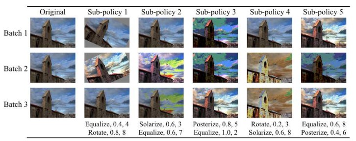
Figure 3. One of the successful policies on ImageNet. As described in the text, most of the policies found on ImageNet used color-based transformations.
图 3|ImageNet 上一条成功的策略。如正文所述,在 ImageNet 上找到的大多数策略使用基于颜色的变换。
Again, we combine the 5 best policies for a total of 25 sub-policies to create the final policy for ImageNet training. We then train on the full ImageNet from scratch with this policy using the ResNet-50 and ResNet-200 models for 270 epochs. We use a batch size of 4096 and a learning rate of 1.6. We decay the learning rate by 10-fold at epochs 90, 180, and 240. For baseline augmentation, we use the standard Inception-style pre-processing which involves scaling pixel values to [-1,1], horizontal flips with 50% probability, and random distortions of colors [22, 59]. For models trained with AutoAugment, we use the baseline pre-processing and the policy learned on ImageNet. We find that removing the random distortions of color does not change the results for AutoAugment.
同样,我们把最好的 5 条策略合并,总共得到 25 条子策略,作为 ImageNet 训练的最终策略。然后我们用该策略从零开始在完整 ImageNet 上训练 ResNet-50 和 ResNet-200 模型,共 270 个轮次。批量大小为 4096,学习率为 1.6。我们在第 90、180 和 240 个轮次把学习率衰减 10 倍。基线增广使用标准的 Inception 风格预处理,包括把像素值缩放到 [-1,1]、以 50% 的概率做水平翻转,以及对颜色做随机扰动 [22, 59]。对用 AutoAugment 训练的模型,我们使用基线预处理以及在 ImageNet 上学到的策略。我们发现,去掉颜色的随机扰动并不会改变 AutoAugment 的结果。
| Model | Inception Pre-processing [59] | AutoAugment ours |
|---|---|---|
| ResNet-50 | 76.3 / 93.1 | 77.6 / 93.8 |
| ResNet-200 | 78.5 / 94.2 | 80.0 / 95.0 |
| AmoebaNet-B (6,190) | 82.2 / 96.0 | 82.8 / 96.2 |
| AmoebaNet-C (6,228) | 83.1 / 96.1 | 83.5 / 96.5 |
Table 3. Validation set Top-1 / Top-5 accuracy (%) on ImageNet. Higher is better. ResNet-50 with baseline augmentation result is taken from [20]. AmoebaNet-B,C results with Inception-style pre-processing are replicated in our experiments and match the previously reported result by [48]. There exists a better result of 85.4% Top-1 error rate [37] but their method makes use of a large amount of weakly labeled extra data. Ref. [68] reports an improvement of 1.5% for a ResNet-50 model.
| 模型 | Inception 预处理 [59] | AutoAugment(本文) |
|---|---|---|
| ResNet-50 | 76.3 / 93.1 | 77.6 / 93.8 |
| ResNet-200 | 78.5 / 94.2 | 80.0 / 95.0 |
| AmoebaNet-B (6,190) | 82.2 / 96.0 | 82.8 / 96.2 |
| AmoebaNet-C (6,228) | 83.1 / 96.1 | 83.5 / 96.5 |
表 3. ImageNet 验证集上的 Top-1 / Top-5 精度(%)。越高越好。带基线增广的 ResNet-50 结果取自 [20]。带 Inception 风格预处理的 AmoebaNet-B、C 结果在我们的实验中得到复现,并与 [48] 先前报告的结果一致。存在一个更好的 85.4% Top-1 错误率结果 [37],但他们的方法使用了大量弱标注的额外数据。文献 [68] 报告,一个 ResNet-50 模型有 1.5% 的改善。
Our ImageNet results are shown in Table 3. As can be seen from the results, AutoAugment improves over the widely-used Inception Pre-processing [59] across a wide range of models, from ResNet-50 to the state-of-art AmoebaNets [48]. Secondly, applying AutoAugment to AmoebaNet-C improves its top-1 and top-5 accuracy from 83.1% / 96.1% to 83.5% / 96.5%. This improvement is remarkable given that the best augmentation policy was discovered on 5,000 images. We expect the results to be even better when more compute is available so that AutoAugment can use more images to discover even better augmentation policies. The accuracy of 83.5% / 96.5% is also the new state-of-art top-1/top-5 accuracy on this dataset (without multicrop / ensembling).
我们的 ImageNet 结果见表 3。从表中可以看到,从 ResNet-50 到当时最好的 AmoebaNets [48],AutoAugment 在很宽的模型范围内都改善了被广泛使用的 Inception 预处理 [59]。其次,把 AutoAugment 用到 AmoebaNet-C 上,将其 Top-1 和 Top-5 精度从 83.1% / 96.1% 提高到 83.5% / 96.5%。考虑到最佳增广策略是在 5,000 张图像上发现的,这一改善相当可观。我们预期,当有更多计算资源、从而使 AutoAugment 能用更多图像去发现更好的增广策略时,结果还会更好。83.5% / 96.5% 的精度也是该数据集上新的当时最高 Top-1 / Top-5 精度(不做多裁剪 / 集成)。
4.3. The Transferability of Learned Augmentation policies to Other Datasets
4.3. 学到的增广策略向其他数据集的可迁移性
In the above, we applied AutoAugment directly to find augmentation policies on the dataset of interest (AutoAugment-direct). In many cases, such application of AutoAugment can be resource-intensive. Here we seek to understand if it is possible to transfer augmentation policies from one dataset to another (which we call AutoAugment-transfer). If such transfer happens naturally, the resource requirements won’t be as intensive as applying AutoAugment directly. Also if such transfer happens naturally, we also have clear evidence that AutoAugment does not “overfit” to the dataset of interest and that AutoAugment indeed finds generic transformations that can be applied to all kinds of problems.
在上面,我们直接应用 AutoAugment,在感兴趣的数据集上寻找增广策略(AutoAugment-direct)。在许多情形里,这样应用 AutoAugment 可能很耗费资源。这里我们想了解,是否有可能把增广策略从一个数据集迁移到另一个数据集(我们称之为 AutoAugment-transfer)。如果这种迁移能够自然发生,资源需求就不会像直接应用 AutoAugment 那样密集。而且,如果这种迁移能够自然发生,我们也有明确证据表明 AutoAugment 并没有对感兴趣的数据集“过拟合”,并且 AutoAugment 的确找到了可以应用到各类问题上的通用变换。
To evaluate the transferability of the policy found on ImageNet, we use the same policy that is learned on ImageNet (and used for the results on Table 3) on five FGVC datasets with image size similar to ImageNet. These datasets are challenging as they have relatively small sets of training examples while having a large number of classes.
为了评估在 ImageNet 上找到的策略的可迁移性,我们把在 ImageNet 上学到的、并用于表 3 结果的同一条策略,用到五个图像尺寸与 ImageNet 相近的 FGVC 数据集上。这些数据集具有挑战性,因为它们的训练样本相对较少,同时类别数很多。
| Dataset | Train Size | Classes | Baseline | AutoAugment-transfer |
|---|---|---|---|---|
| Oxford 102 Flowers [43] | 2,040 | 102 | 6.7 | 4.6 |
| Caltech-101 [15] | 3,060 | 102 | 19.4 | 13.1 |
| Oxford-IIIT Pets [14] | 3,680 | 37 | 13.5 | 11.0 |
| FGVC Aircraft [38] | 6,667 | 100 | 9.1 | 7.3 |
| Stanford Cars [27] | 8,144 | 196 | 6.4 | 5.2 |
Table 4. Test set Top-1 error rates (%) on FGVC datasets for Inception v4 models trained from scratch with and without AutoAugment-transfer. Lower rates are better. AutoAugment-transfer results use the policy found on ImageNet. Baseline models used Inception pre-processing.
| 数据集 | 训练集大小 | 类别数 | 基线 | AutoAugment-transfer |
|---|---|---|---|---|
| Oxford 102 Flowers [43] | 2,040 | 102 | 6.7 | 4.6 |
| Caltech-101 [15] | 3,060 | 102 | 19.4 | 13.1 |
| Oxford-IIIT Pets [14] | 3,680 | 37 | 13.5 | 11.0 |
| FGVC Aircraft [38] | 6,667 | 100 | 9.1 | 7.3 |
| Stanford Cars [27] | 8,144 | 196 | 6.4 | 5.2 |
表 4. 从零训练的 Inception v4 模型在 FGVC 数据集上、使用与不使用 AutoAugment-transfer 时的测试集 Top-1 错误率(%)。越低越好。AutoAugment-transfer 的结果使用在 ImageNet 上找到的策略。基线模型使用 Inception 预处理。
For all of the datasets listed in Table 4, we train a Inception v4 [58] for 1,000 epochs, using a cosine learning rate decay with one annealing cycle. The learning rate and weight decay are chosen based on the validation set performance. We then combine the training set and the validation set and train again with the chosen hyperparameters. The image size is set to 448x448 pixels. The policies found on ImageNet improve the generalization accuracy of all of the FGVC datasets significantly. To the best of our knowledge, our result on the Stanford Cars dataset is the lowest error rate achieved on this dataset although we train the network weights from scratch. Previous state-of-the-art fine-tuned pre-trained weights on ImageNet and used deep layer aggregation to attain a 5.9% error rate [66].
对表 4 中列出的全部数据集,我们训练一个 Inception v4 [58],共 1,000 个轮次,使用带一个退火周期的余弦学习率衰减。学习率和权重衰减根据验证集表现来选择。随后我们把训练集和验证集合并,再用选定的超参数重新训练。图像大小设为 448×448 像素。在 ImageNet 上找到的策略显著改善了所有这些 FGVC 数据集的泛化精度。据我们所知,尽管我们是从零训练网络权重,斯坦福汽车数据集上的这一结果是该数据集上达到的最低错误率。此前最好结果是在 ImageNet 预训练权重上做微调,并使用深层聚合,达到 5.9% 的错误率 [66]。
5. Discussion
5. 讨论
In this section, we compare our search to previous attempts at automated data augmentation methods. We also discuss the dependence of our results on some of the design decisions we have made through several ablation experiments.
本节把我们的搜索与此前自动化数据增广方法的尝试相比较。我们还通过若干消融实验,讨论结果对我们所做某些设计决策的依赖。
AutoAugment vs. other automated data augmentation methods: Most notable amongst many previous data augmentation methods is the work of [47]. The setup in [47] is similar to GANs [18]: a generator learns to propose augmentation policy (a sequence of image processing operations) such that the augmented images can fool a discriminator. The difference of our method to theirs is that our method tries to optimize classification accuracy directly whereas their method just tries to make sure the augmented images are similar to the current training images.
AutoAugment 与其他自动化数据增广方法:在许多先前的数据增广方法中,最值得注意的是 [47] 的工作。[47] 中的设定类似于 GAN [18]:一个生成器学习提出增广策略(一系列图像处理操作),使得增广后的图像能够骗过判别器。我们的方法与他们的不同之处在于:我们的方法试图直接优化分类精度,而他们的方法只是试图保证增广后的图像与当前训练图像相似。
To make the comparison fair, we carried out experiments similar to that described in [47]. We trained a ResNet-32 and a ResNet-56 using the same policy from Section 4.1, to compare our method to the results from [47]. By training a ResNet-32 with Baseline data augmentation, we achieve the same error as [47] did with ResNet-56 (called Heur. in [47]). For this reason, we trained both a ResNet-32 and a ResNet-56. We show that for both models, AutoAugment leads to higher improvement (∼3.0%).
为了使比较公平,我们进行了与 [47] 中描述类似的实验。我们用第 4.1 节中的同一条策略训练 ResNet-32 和 ResNet-56,以便把本方法与 [47] 的结果相比较。用基线数据增广训练 ResNet-32 时,我们达到了与 [47] 用 ResNet-56 相同的错误率(在 [47] 中称为 Heur.)。因此,我们同时训练了 ResNet-32 和 ResNet-56。我们表明,对这两种模型,AutoAugment 都带来了更高的改善(约 3.0%)。
| Method | Baseline | Augmented | Improvement ∆ |
|---|---|---|---|
| LSTM [47] | 7.7 | 6.0 | 1.6 |
| MF [47] | 7.7 | 5.6 | 2.1 |
| AutoAugment (ResNet-32) | 7.7 | 4.5 | 3.2 |
| AutoAugment (ResNet-56) | 6.6 | 3.6 | 3.0 |
Table 5. The test set error rates (%) on CIFAR-10 with different approaches for automated data augmentation. The MF and LSTM results are taken from [47], and they are for a ResNet-56.
| 方法 | 基线 | 增广后 | 改善 ∆ |
|---|---|---|---|
| LSTM [47] | 7.7 | 6.0 | 1.6 |
| MF [47] | 7.7 | 5.6 | 2.1 |
| AutoAugment (ResNet-32) | 7.7 | 4.5 | 3.2 |
| AutoAugment (ResNet-56) | 6.6 | 3.6 | 3.0 |
表 5. 不同自动化数据增广方法在 CIFAR-10 上的测试集错误率(%)。MF 和 LSTM 的结果取自 [47],它们针对的是 ResNet-56。
Relation between training steps and number of sub-policies: An important aspect of our work is the stochastic application of sub-policies during training. Every image is only augmented by one of the many sub-policies available in each mini-batch, which itself has further stochasticity since each transformation has a probability of application associated with it. We find that this stochasticity requires a certain number of epochs per sub-policy for AutoAugment to be effective. Since the child models are each trained with 5 sub-policies, they need to be trained for more than 80-100 epochs before the model can fully benefit from all of the sub-policies. This is the reason we choose to train our child models for 120 epochs. Each sub-policy needs to be applied a certain number of times before the model benefits from it. After the policy is learned, the full model is trained for longer (e.g. 1800 epochs for Shake-Shake on CIFAR-10, and 270 epochs for ResNet-50 on ImageNet), which allows us to use more sub-policies.
训练步数与子策略数目的关系:我们工作的一个重要方面,是训练过程中子策略的随机施加。每张图像在每个小批量里只被许多可用子策略中的一条所增广,而这条子策略本身还有进一步的随机性,因为每种变换都带有施加概率。我们发现,这种随机性要求每个子策略对应一定数目的训练轮次,AutoAugment 才能有效。由于每个子模型都用 5 条子策略训练,它们需要训练超过 80–100 个轮次,模型才能充分受益于全部子策略。这就是我们选择把子模型训练 120 个轮次的原因。每条子策略都需要被施加一定次数,模型才能从中受益。策略学到之后,完整模型会训练更长时间(例如 CIFAR-10 上的 Shake-Shake 为 1800 个轮次,ImageNet 上的 ResNet-50 为 270 个轮次),这使我们能够使用更多子策略。
Transferability across datasets and architectures: It is important to note that the policies described above transfer well to many model architectures and datasets. For example, the policy learned on Wide-ResNet-40-2 and reduced CIFAR-10 leads to the improvements described on all of the other model architectures trained on full CIFAR-10 and CIFAR-100. Similarly, a policy learned on Wide-ResNet-40-2 and reduced ImageNet leads to significant improvements on Inception v4 trained on FGVC datasets that have different data and class distributions. AutoAugment policies are never found to hurt the performance of models even if they are learned on a different dataset, which is not the case for Cutout on reduced SVHN (Table 2). We present the best policy on ImageNet and SVHN in the Appendix, which can hopefully help researchers improve their generalization accuracy on relevant image classification tasks.
跨数据集与跨架构的可迁移性:需要指出的是,上面描述的策略可以很好地迁移到许多模型架构和数据集。例如,在 Wide-ResNet-40-2 和缩小的 CIFAR-10 上学到的策略,带来了在完整 CIFAR-10 和 CIFAR-100 上训练的所有其他模型架构中所描述的那些改善。类似地,在 Wide-ResNet-40-2 和缩小的 ImageNet 上学到的策略,在数据分布和类别分布都不同的 FGVC 数据集上训练的 Inception v4 上也带来了显著改善。即使策略是在不同数据集上学到的,也从未发现 AutoAugment 策略会损害模型性能,而这并不是 Cutout 在缩小的 SVHN 上的情况(表 2)。我们在附录中给出了 ImageNet 和 SVHN 上的最佳策略,希望能帮助研究者提高相关图像分类任务上的泛化精度。
Despite the observed transferability, we find that policies learned on data distributions closest to the target yield the best performance: when training on SVHN, using the best policy learned on reduced CIFAR-10 does slightly improve generalization accuracy compared to the baseline augmentation, but not as significantly as applying the SVHN-learned policy.
尽管观察到了可迁移性,我们发现在最接近目标的数据分布上学到的策略会给出最好的表现:在 SVHN 上训练时,使用在缩小的 CIFAR-10 上学到的最佳策略,相比基线增广会略微改善泛化精度,但不如施加在 SVHN 上自己学到的策略来得显著。
5.1. Ablation experiments
5.1. 消融实验
Changing the number of sub-policies: Our hypothesis is that as we increase the number of sub-policies, the neural network is trained on the same points with a greater diversity of augmentation, which should increase the generalization accuracy. To test this hypothesis, we investigate the average validation accuracy of fully-trained Wide-ResNet-28-10 models on CIFAR-10 as a function of the number of sub-policies used in training. We randomly select sub-policy sets from a pool of 500 good sub-policies, and train the Wide-ResNet-28-10 model for 200 epochs with each of these sub-policy sets. For each set size, we sampled sub-policies five different times for better statistics. The training details of the model are the same as above for Wide-ResNet-28-10 trained on CIFAR-10. Figure 4 shows the average validation set accuracy as a function of the number of sub-policies used in training, confirming that the validation accuracy improves with more sub-policies up to about 20 sub-policies.
改变子策略的数目:我们的假设是,随着子策略数目增加,神经网络会在相同的点上接受更多样的增广训练,从而应能提高泛化精度。为了检验这一假设,我们考察在 CIFAR-10 上充分训练的 Wide-ResNet-28-10 模型的平均验证精度,如何随训练中使用的子策略数目变化。我们从 500 条较好的子策略池中随机选取子策略集合,并用每个这样的子策略集合把 Wide-ResNet-28-10 模型训练 200 个轮次。对每种集合大小,我们把子策略采样五次,以得到更好的统计。模型的训练细节与上面在 CIFAR-10 上训练 Wide-ResNet-28-10 时相同。图 4 给出平均验证集精度随训练中所用子策略数目的变化,确认验证精度会随着子策略增多而提高,直到大约 20 条子策略。
Randomizing the probabilities and magnitudes in the augmentation policy: We take the AutoAugment policy on CIFAR-10 and randomize the probabilities and magnitudes of each operation in it. We train a Wide-ResNet-28-10 [67], using the same training procedure as before, for 20 different instances of the randomized probabilities and magnitudes. We find the average error to be 3.0% (with a standard deviation of 0.1%), which is 0.4% worse than the result achieved with the original AutoAugment policy (see Table 2).
随机化增广策略中的概率和幅度:我们取 CIFAR-10 上的 AutoAugment 策略,并随机化其中每个操作的概率和幅度。我们用与此前相同的训练程序,对 20 组不同的随机化概率和幅度,训练 Wide-ResNet-28-10 [67]。我们发现平均错误率为 3.0%(标准差为 0.1%),比使用原来的 AutoAugment 策略所得到的结果差 0.4%(见表 2)。
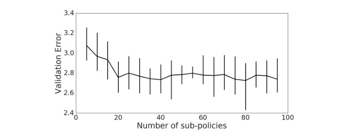
Figure 4. Validation error (averaged over 5 runs) of Wide-ResNet-28-10 trained on CIFAR-10 as a function of number of randomly selected sub-policies (out of a pool of 500 good sub-policies) used in training with AutoAugment. Bars represent the range of validation errors for each number.
图 4|在 CIFAR-10 上训练的 Wide-ResNet-28-10 的验证错误率(对 5 次运行取平均),随 AutoAugment 训练中使用的、从 500 条较好子策略池中随机选取的子策略数目变化。误差条表示每个数目下验证错误率的范围。
Performance of random policies: Next, we randomize the whole policy, the operations as well as the probabilities and magnitudes. Averaged over 20 runs, this experiment yields an average accuracy of 3.1% (with a standard deviation of 0.1%), which is slightly worse than randomizing only the probabilities and magnitudes. The best random policy achieves achieves an error of 3.0% (when average over 5 independent runs). This shows that even AutoAugment with randomly sampled policy leads to appreciable improvements.
随机策略的表现:接下来,我们随机化整条策略,包括操作以及概率和幅度。对 20 次运行取平均,该实验得到的平均错误率为 3.1%(标准差为 0.1%),略差于只随机化概率和幅度。最好的随机策略达到 3.0% 的错误率(对 5 次独立运行取平均)。这表明,即便是带有随机采样策略的 AutoAugment,也能带来可观的改善。
The ablation experiments indicate that even data augmentation policies that are randomly sampled from our search space can lead to improvements on CIFAR-10 over the baseline augmentation policy. However, the improvements exhibited by random policies are less than those shown by the AutoAugment policy (2.6% ± 0.1% vs. 3.0% ± 0.1% error rate). Furthermore, the probability and magnitude information learned within the AutoAugment policy seem to be important, as its effectiveness is reduced significantly when those parameters are randomized. We emphasize again that we trained our controller using RL out of convenience, augmented random search and evolutionary strategies can be used just as well. The main contribution of this paper is in our approach to data augmentation and in the construction of the search space; not in discrete optimization methodology.
消融实验表明,即便是从我们的搜索空间中随机采样的数据增广策略,也能在 CIFAR-10 上相对基线增广策略带来改善。不过,随机策略所表现出的改善小于 AutoAugment 策略(错误率为 2.6% ± 0.1% 对 3.0% ± 0.1%)。此外,AutoAugment 策略中学到的概率和幅度信息看来是重要的,因为当这些参数被随机化时,其有效性会显著下降。我们再次强调,用强化学习训练控制器是出于方便,增强随机搜索和进化策略同样可以使用。本文的主要贡献在于我们对数据增广的处理方式以及搜索空间的构造,而不在离散优化方法本身。
6. Acknowledgments
6. 致谢
We thank Alok Aggarwal, Gabriel Bender, Yanping Huang, Pieter-Jan Kindermans, Simon Kornblith, Augustus Odena, Avital Oliver, Colin Raffel, and Jonathan Shlens for helpful discussions.
我们感谢 Alok Aggarwal、Gabriel Bender、Yanping Huang、Pieter-Jan Kindermans、Simon Kornblith、Augustus Odena、Avital Oliver、Colin Raffel 和 Jonathan Shlens 的有益讨论。
References
参考文献
[1] M. Abadi, P. Barham, J. Chen, Z. Chen, A. Davis, J. Dean, M. Devin, S. Ghemawat, G. Irving, M. Isard, M. Kudlur, J. Levenberg, R. Monga, S. Moore, D. G. Murray, B. Steiner, P. Tucker, V. Vasudevan, P. Warden, M. Wicke, Y. Yu, and X. Zheng. Tensorflow: A system for large-scale machine learning. In Proceedings of the 12th USENIX Conference on Operating Systems Design and Implementation, OSDI’16, pages 265–283, Berkeley, CA, USA, 2016. USENIX Association. 5
[2] A. Antoniou, A. Storkey, and H. Edwards. Data augmentation generative adversarial networks. arXiv preprint arXiv:1711.04340, 2017. 2
[3] H. S. Baird. Document image defect models. In Structured Document Image Analysis, pages 546–556. Springer, 1992. 1
[4] B. Baker, O. Gupta, N. Naik, and R. Raskar. Designing neural network architectures using reinforcement learning. In International Conference on Learning Representations, 2017. 2, 3
[5] I. Bello, B. Zoph, V. Vasudevan, and Q. V. Le. Neural optimizer search with reinforcement learning. In International Conference on Machine Learning, 2017. 3
[6] J. Bergstra and Y. Bengio. Random search for hyperparameter optimization. Journal of Machine Learning Research, 13(Feb):281–305, 2012. 4
[7] A. Brock, T. Lim, J. M. Ritchie, and N. Weston. Smash: one-shot model architecture search through hypernetworks. In International Conference on Learning Representations, 2017. 2
[8] D. Ciregan, U. Meier, and J. Schmidhuber. Multi-column deep neural networks for image classification. In Proceedings of IEEE Conference on Computer Vision and Pattern Recognition, pages 3642–3649. IEEE, 2012. 2
[9] E. D. Cubuk, B. Zoph, S. S. Schoenholz, and Q. V. Le. Intriguing properties of adversarial examples. arXiv preprint arXiv:1711.02846, 2017. 2
[10] J. Deng, W. Dong, R. Socher, L.-J. Li, K. Li, and L. Fei-Fei. Imagenet: A large-scale hierarchical image database. In Proceedings of IEEE Conference on Computer Vision and Pattern Recognition (CVPR), 2009. 4
[11] T. DeVries and G. W. Taylor. Dataset augmentation in feature space. arXiv preprint arXiv:1702.05538, 2017. 2
[12] T. DeVries and G. W. Taylor. Improved regularization of convolutional neural networks with cutout. arXiv preprint arXiv:1708.04552, 2017. 2, 3, 4, 5, 6, 13
[13] T. Elsken, J.-H. Metzen, and F. Hutter. Simple and efficient architecture search for convolutional neural networks. arXiv preprint arXiv:1711.04528, 2017. 2
[14] Y. Em, F. Gag, Y. Lou, S. Wang, T. Huang, and L.-Y. Duan. Incorporating intra-class variance to fine-grained visual recognition. In Multimedia and Expo (ICME), 2017 IEEE International Conference on, pages 1452–1457. IEEE, 2017. 7
[15] L. Fei-Fei, R. Fergus, and P. Perona. Learning generative visual models from few training examples: An incremental bayesian approach tested on 101 object categories. Computer vision and Image understanding, 106(1):59–70, 2007. 7
[16] K. Fukushima and S. Miyake. Neocognitron: A self-organizing neural network model for a mechanism of visual pattern recognition. In Competition and cooperation in neural nets, pages 267–285. Springer, 1982. 1
[17] X. Gastaldi. Shake-shake regularization. arXiv preprint arXiv:1705.07485, 2017. 4, 5, 6
[18] I. Goodfellow, J. Pouget-Abadie, M. Mirza, B. Xu, D. Warde-Farley, S. Ozair, A. Courville, and Y. Bengio. Generative adversarial nets. In Advances in neural information processing systems, pages 2672–2680, 2014. 7
[19] D. Han, J. Kim, and J. Kim. Deep pyramidal residual networks. In Proceedings of IEEE Conference on Computer Vision and Pattern Recognition (CVPR), pages 6307–6315. IEEE, 2017. 1
[20] K. He, X. Zhang, S. Ren, and J. Sun. Deep residual learning for image recognition. In Proceedings of the IEEE Conference on Computer Vision and Pattern Recognition (CVPR), pages 770–778, 2016. 1, 6
[21] S. Hochreiter and J. Schmidhuber. Long short-term memory. Neural computation, 9(8):1735–1780, 1997. 4
[22] A. G. Howard. Some improvements on deep convolutional neural network based image classification. arXiv preprint arXiv:1312.5402, 2013. 6
[23] J. Hu, L. Shen, and G. Sun. Squeeze-and-excitation networks. arXiv preprint arXiv:1709.01507, 2017. 1
[24] H. Inoue. Data augmentation by pairing samples for images classification. arXiv preprint arXiv:1801.02929, 2018. 3, 13
[25] K. Jarrett, K. Kavukcuoglu, Y. LeCun, et al. What is the best multi-stage architecture for object recognition? In Proceedings of IEEE Conference on Computer Vision and Pattern Recognition, pages 2146–2153. IEEE, 2009. 1
[26] S. Kornblith, J. Shlens, and Q. V. Le. Do better imagenet models transfer better? arXiv preprint arXiv:1805.08974, 2018. 2
[27] J. Krause, J. Deng, M. Stark, and L. Fei-Fei. Collecting a large-scale dataset of fine-grained cars. In Second Workshop on Fine-Grained Visual Categorization, 2013. 2, 7
[28] A. Krizhevsky and G. Hinton. Learning multiple layers of features from tiny images. Technical report, University of Toronto, 2009. 4
[29] A. Krizhevsky, I. Sutskever, and G. E. Hinton. Imagenet classification with deep convolutional neural networks. In Advances in Neural Information Processing Systems, 2012. 1, 2
[30] M. Kumar, G. E. Dahl, V. Vasudevan, and M. Norouzi. Parallel architecture and hyperparameter search via successive halving and classification. arXiv preprint arXiv:1805.10255, 2018. 4
[31] S. Laine and T. Aila. Temporal ensembling for semi-supervised learning. arXiv preprint arXiv:1610.02242, 2016. 5
[32] Y. LeCun, L. Bottou, Y. Bengio, and P. Haffner. Gradient-based learning applied to document recognition. Proceedings of the IEEE, 86(11):2278–2324, 1998. 1
[33] J. Lemley, S. Bazrafkan, and P. Corcoran. Smart augmentation learning an optimal data augmentation strategy. IEEE Access, 5:5858–5869, 2017. 2
[34] C. Liu, B. Zoph, J. Shlens, W. Hua, L.-J. Li, L. Fei-Fei, A. Yuille, J. Huang, and K. Murphy. Progressive neural architecture search. arXiv preprint arXiv:1712.00559, 2017. 2
[35] H. Liu, K. Simonyan, O. Vinyals, C. Fernando, and K. Kavukcuoglu. Hierarchical representations for efficient architecture search. In International Conference on Learning Representations, 2018. 2
[36] I. Loshchilov and F. Hutter. SGDR: Stochastic gradient descent with warm restarts. arXiv preprint arXiv:1608.03983, 2016. 4
[37] D. Mahajan, R. Girshick, V. Ramanathan, K. He, M. Paluri, Y. Li, A. Bharambe, and L. van der Maaten. Exploring the limits of weakly supervised pretraining. arXiv preprint arXiv:1805.00932, 2018. 6
[38] S. Maji, E. Rahtu, J. Kannala, M. Blaschko, and A. Vedaldi. Fine-grained visual classification of aircraft. arXiv preprint arXiv:1306.5151, 2013. 2, 7
[39] H. Mania, A. Guy, and B. Recht. Simple random search provides a competitive approach to reinforcement learning. arXiv preprint arXiv:1803.07055, 2018. 2
[40] T. Miyato, S.-i. Maeda, M. Koyama, and S. Ishii. Virtual adversarial training: a regularization method for supervised and semi-supervised learning. In International Conference on Learning Representations, 2016. 5, 6
[41] S. Mun, S. Park, D. K. Han, and H. Ko. Generative adversarial network based acoustic scene training set augmentation and selection using svm hyper-plane. In Detection and Classification of Acoustic Scenes and Events Workshop, 2017. 2
[42] Y. Netzer, T. Wang, A. Coates, A. Bissacco, B. Wu, and A. Y. Ng. Reading digits in natural images with unsupervised feature learning. In NIPS Workshop on Deep Learning and Unsupervised Feature Learning, 2011. 4, 5
[43] M.-E. Nilsback and A. Zisserman. Automated flower classification over a large number of classes. In Computer Vision, Graphics & Image Processing, 2008. ICVGIP’08. Sixth Indian Conference on, pages 722–729. IEEE, 2008. 7
[44] A. Oliver, A. Odena, C. Raffel, E. D. Cubuk, and I. J. Goodfellow. Realistic evaluation of deep semi-supervised learning algorithms. arXiv preprint arXiv:1804.09170, 2018. 5
[45] L. Perez and J. Wang. The effectiveness of data augmentation in image classification using deep learning. arXiv preprint arXiv:1712.04621, 2017. 2
[46] H. Pham, M. Y. Guan, B. Zoph, Q. V. Le, and J. Dean. Efficient neural architecture search via parameter sharing. In International Conference on Machine Learning, 2018. 2
[47] A. J. Ratner, H. Ehrenberg, Z. Hussain, J. Dunnmon, and C. R´e. Learning to compose domain-specific transformations for data augmentation. In Advances in Neural Information Processing Systems, pages 3239–3249, 2017. 2, 7
[48] E. Real, A. Aggarwal, Y. Huang, and Q. V. Le. Regularized evolution for image classifier architecture search. arXiv preprint arXiv:1802.01548, 2018. 1, 2, 4, 5, 6
[49] E. Real, S. Moore, A. Selle, S. Saxena, Y. L. Suematsu, J. Tan, Q. Le, and A. Kurakin. Large-scale evolution of image classifiers. In International Conference on Machine Learning, 2017. 2
[50] B. Recht, R. Roelofs, L. Schmidt, and V. Shankar. Do cifar-10 classifiers generalize to cifar-10? arXiv preprint arXiv:1806.00451, 2018. 5
[51] M. Sajjadi, M. Javanmardi, and T. Tasdizen. Regularization with stochastic transformations and perturbations for deep semi-supervised learning. In Advances in Neural Information Processing Systems, pages 1163–1171, 2016. 5
[52] I. Sato, H. Nishimura, and K. Yokoi. Apac: Augmented pattern classification with neural networks. arXiv preprint arXiv:1505.03229, 2015. 2
[53] J. Schulman, F. Wolski, P. Dhariwal, A. Radford, and O. Klimov. Proximal policy optimization algorithms. arXiv preprint arXiv:1707.06347, 2017. 3, 4
[54] P. Y. Simard, D. Steinkraus, J. C. Platt, et al. Best practices for convolutional neural networks applied to visual document analysis. In Proceedings of International Conference on Document Analysis and Recognition, 2003. 1, 2
[55] K. Simonyan and A. Zisserman. Very deep convolutional networks for large-scale image recognition. Advances in Neural Information Processing Systems, 2015. 1
[56] L. Sixt, B. Wild, and T. Landgraf. Rendergan: Generating realistic labeled data. arXiv preprint arXiv:1611.01331, 2016. 2
[57] I. Sutskever, J. Schulman, T. Salimans, and D. Kingma. Requests For Research 2.0. https://blog.openai. com/requests-for-research-2, 2018. 1
[58] C. Szegedy, S. Ioffe, V. Vanhoucke, and A. A. Alemi. Inception-v4, inception-resnet and the impact of residual connections on learning. In AAAI, 2017. 1, 7
[59] C. Szegedy, W. Liu, Y. Jia, P. Sermanet, S. Reed, D. Anguelov, D. Erhan, V. Vanhoucke, A. Rabinovich, et al. Going deeper with convolutions. In Proceedings of the IEEE Conference on Computer Vision and Pattern Recognition (CVPR), 2015. 1, 6
[60] A. Tarvainen and H. Valpola. Mean teachers are better role models: Weight-averaged consistency targets improve semi-supervised deep learning results. In Advances in neural information processing systems, pages 1195–1204, 2017. 5
[61] T. Tran, T. Pham, G. Carneiro, L. Palmer, and I. Reid. A bayesian data augmentation approach for learning deep models. In Advances in Neural Information Processing Systems, pages 2794–2803, 2017. 2
[62] L. Wan, M. Zeiler, S. Zhang, Y. Le Cun, and R. Fergus. Regularization of neural networks using dropconnect. In International Conference on Machine Learning, pages 1058–1066, 2013. 2
[63] L. Xie and A. Yuille. Genetic CNN. In Proceedings of IEEE Conference on Computer Vision and Pattern Recognition, 2017. 2
[64] S. Xie, R. Girshick, P. Doll´ar, Z. Tu, and K. He. Aggregated residual transformations for deep neural networks. In Proceedings of IEEE Conference on Computer Vision and Pattern Recognition (CVPR), pages 5987–5995, 2017. 1
[65] Y. Yamada, M. Iwamura, and K. Kise. Shakedrop regularization. arXiv preprint arXiv:1802.02375, 2018. 4, 5, 6
[66] F. Yu, D. Wang, and T. Darrell. Deep layer aggregation. arXiv preprint arXiv:1707.06484, 2017. 1, 7
[67] S. Zagoruyko and N. Komodakis. Wide residual networks. In British Machine Vision Conference, 2016. 4, 5, 6, 8
[68] H. Zhang, M. Cisse, Y. N. Dauphin, and D. Lopez-Paz. mixup: Beyond empirical risk minimization. arXiv preprint arXiv:1710.09412, 2017. 5, 6, 13
[69] Z. Zhong, L. Zheng, G. Kang, S. Li, and Y. Yang. Random erasing data augmentation. arXiv preprint arXiv:1708.04896, 2017. 13
[70] X. Zhu, Y. Liu, Z. Qin, and J. Li. Data augmentation in emotion classification using generative adversarial networks. arXiv preprint arXiv:1711.00648, 2017. 2
[71] B. Zoph and Q. V. Le. Neural architecture search with reinforcement learning. In International Conference on Learning Representations, 2017. 2, 3
[72] B. Zoph, V. Vasudevan, J. Shlens, and Q. V. Le. Learning transferable architectures for scalable image recognition. In Proceedings of IEEE Conference on Computer Vision and Pattern Recognition, 2017. 1, 2, 3, 4