Mastering the game of Go without human knowledge

不借助人类知识精通围棋

David Silver*, Julian Schrittwieser*, Karen Simonyan*, Ioannis Antonoglou, Aja Huang, Arthur Guez, Thomas Hubert, Lucas Baker, Matthew Lai, Adrian Bolton, Yutian Chen, Timothy Lillicrap, Fan Hui, Laurent Sifre, George van den Driessche, Thore Graepel, Demis Hassabis.

DeepMind, 5 New Street Square, London EC4A 3TW.

*These authors contributed equally to this work.

A long-standing goal of artificial intelligence is an algorithm that learns, tabula rasa, superhuman proficiency in challenging domains. Recently, AlphaGo became the first program to defeat a world champion in the game of Go. The tree search in AlphaGo evaluated positions and selected moves using deep neural networks. These neural networks were trained by supervised learning from human expert moves, and by reinforcement learning from self-play. Here, we introduce an algorithm based solely on reinforcement learning, without human data, guidance, or domain knowledge beyond game rules. AlphaGo becomes its own teacher: a neural network is trained to predict AlphaGo's own move selections and also the winner of AlphaGo's games. This neural network improves the strength of tree search, resulting in higher quality move selection and stronger self-play in the next iteration. Starting tabula rasa, our new program AlphaGo Zero achieved superhuman performance, winning 100-0 against the previously published, champion-defeating AlphaGo.

人工智能的一个长期目标，是让算法从一张白纸（tabula rasa）出发，在高难度领域达到超人水平。不久前，AlphaGo 成为第一个在围棋中击败世界冠军的程序。它的树搜索用深度神经网络来评估局面、选择着法。这些网络既用人类高手的着法做监督学习，也用自我对弈做强化学习。本文提出一种只靠强化学习的算法，不使用人类数据、人工指导，也不使用规则之外的领域知识。AlphaGo 成为自己的老师：一个神经网络被训练去预测 AlphaGo 自己选出的着法，以及对局的胜者。这个网络会增强树搜索，从而在下一轮迭代里选出更好的着法、下出更强的自我对弈。新程序 AlphaGo Zero 从白纸起步，达到了超人水平，并以 100 比 0 击败此前发表、曾战胜世界冠军的 AlphaGo。

Much progress towards artificial intelligence has been made using supervised learning systems that are trained to replicate the decisions of human experts. However, expert data is often expensive, unreliable, or simply unavailable. Even when reliable data is available it may impose a ceiling on the performance of systems trained in this manner. In contrast, reinforcement learning systems are trained from their own experience, in principle allowing them to exceed human capabilities, and to operate in domains where human expertise is lacking. Recently, there has been rapid progress towards this goal, using deep neural networks trained by reinforcement learning. These systems have outperformed humans in computer games such as Atari and 3D virtual environments. However, the most challenging domains in terms of human intellect — such as the game of Go, widely viewed as a grand challenge for artificial intelligence — require precise and sophisticated lookahead in vast search spaces. Fully general methods have not previously achieved human-level performance in these domains.

面向人工智能的许多进展，来自训练系统去复现人类专家决策的监督学习。不过，专家数据往往昂贵、不可靠，甚至根本拿不到。即便有可靠数据，按这种方式训练的系统也可能被数据本身钉死在一个上限上。相比之下，强化学习系统从自身经验中训练，原则上可以超过人类能力，也能在缺少人类专长的领域运作。近来，用强化学习训练深度神经网络，在这条路上进展很快。这些系统已经在 Atari 等电子游戏和三维虚拟环境中超过人类。可是，就人类智识而言最具挑战的领域——例如被广泛视为人工智能重大考验的围棋——需要在巨大搜索空间里做精确而复杂的前瞻。此前，完全通用的方法还没有在这些领域达到人类水平。

AlphaGo was the first program to achieve superhuman performance in Go. The published version, which we refer to as AlphaGo Fan, defeated the European champion Fan Hui in October 2015. AlphaGo Fan utilised two deep neural networks: a policy network that outputs move probabilities, and a value network that outputs a position evaluation. The policy network was trained initially by supervised learning to accurately predict human expert moves, and was subsequently refined by policy-gradient reinforcement learning. The value network was trained to predict the winner of games played by the policy network against itself. Once trained, these networks were combined with a Monte-Carlo Tree Search (MCTS) to provide a lookahead search, using the policy network to narrow down the search to high-probability moves, and using the value network (in conjunction with Monte-Carlo rollouts using a fast rollout policy) to evaluate positions in the tree. A subsequent version, which we refer to as AlphaGo Lee, used a similar approach (see Methods), and defeated Lee Sedol, the winner of 18 international titles, in March 2016.

AlphaGo 是第一个在围棋中达到超人水平的程序。已发表的版本我们称作 AlphaGo Fan，它在 2015 年 10 月击败了欧洲冠军 Fan Hui。AlphaGo Fan 使用两个深度神经网络：输出着法概率的策略网络，以及输出局面评估的价值网络。策略网络先用监督学习准确预测人类高手着法，再通过策略梯度强化学习加以改进。价值网络则训练去预测策略网络自我对弈的胜者。训练完成后，这两个网络与蒙特卡洛树搜索（MCTS）结合，提供前瞻搜索：策略网络把搜索收窄到高概率着法，价值网络（再配合用快速走子策略做的蒙特卡洛走子）评估树中的局面。随后的版本我们称作 AlphaGo Lee，方法相近（见 Methods），并在 2016 年 3 月击败了拥有 18 个国际冠军头衔的 Lee Sedol。

Our program, AlphaGo Zero, differs from AlphaGo Fan and AlphaGo Lee in several important aspects. First and foremost, it is trained solely by self-play reinforcement learning, starting from random play, without any supervision or use of human data. Second, it only uses the black and white stones from the board as input features. Third, it uses a single neural network, rather than separate policy and value networks. Finally, it uses a simpler tree search that relies upon this single neural network to evaluate positions and sample moves, without performing any Monte-Carlo rollouts. To achieve these results, we introduce a new reinforcement learning algorithm that incorporates lookahead search inside the training loop, resulting in rapid improvement and precise and stable learning. Further technical differences in the search algorithm, training procedure and network architecture are described in Methods.

我们的程序 AlphaGo Zero 与 AlphaGo Fan、AlphaGo Lee 有几处重要不同。首先也是最主要的一点：它只靠自我对弈强化学习训练，从随机走子出发，不用任何监督，也不使用人类数据。第二，输入特征只用棋盘上的黑白子。第三，它使用单一神经网络，而不再分开策略网络和价值网络。最后，它的树搜索更简单，只靠这一个网络评估局面并采样着法，不再做任何蒙特卡洛走子。为了达到这些结果，我们提出一种把前瞻搜索嵌进训练循环的新强化学习算法，学习既快又稳定、精度也高。搜索算法、训练流程和网络结构上的更多技术差异见 Methods。

Reinforcement Learning in AlphaGo Zero

AlphaGo Zero 中的强化学习

Our new method uses a deep neural network $f_\theta$ with parameters $\theta$. This neural network takes as an input the raw board representation $s$ of the position and its history, and outputs both move probabilities and a value, $(p, v) = f_\theta(s)$. The vector of move probabilities $p$ represents the probability of selecting each move (including pass), $p_a = \Pr(a|s)$. The value $v$ is a scalar evaluation, estimating the probability of the current player winning from position $s$. This neural network combines the roles of both policy network and value network into a single architecture. The neural network consists of many residual blocks of convolutional layers with batch normalisation and rectifier non-linearities (see Methods).

我们的新方法使用带参数 $\theta$ 的深度神经网络 $f_\theta$。网络的输入是局面及其历史的原始棋盘表示 $s$，输出则同时给出着法概率和价值，$(p, v) = f_\theta(s)$。着法概率向量 $p$ 表示选择每一步（包括停着）的概率，$p_a = \Pr(a|s)$。价值 $v$ 是一个标量评估，估计当前执棋方从局面 $s$ 获胜的概率。这个网络把策略网络和价值网络的角色合并进同一套结构。网络由许多带批归一化和整流非线性的卷积残差块组成（见 Methods）。

The neural network in AlphaGo Zero is trained from games of self-play by a novel reinforcement learning algorithm. In each position $s$, an MCTS search is executed, guided by the neural network $f_\theta$. The MCTS search outputs probabilities $\pi$ of playing each move. These search probabilities usually select much stronger moves than the raw move probabilities $p$ of the neural network $f_\theta(s)$; MCTS may therefore be viewed as a powerful policy improvement operator. Self-play with search — using the improved MCTS-based policy to select each move, then using the game winner $z$ as a sample of the value — may be viewed as a powerful policy evaluation operator. The main idea of our reinforcement learning algorithm is to use these search operators repeatedly in a policy iteration procedure: the neural network's parameters are updated to make the move probabilities and value $(p, v) = f_\theta(s)$ more closely match the improved search probabilities and self-play winner $(\pi, z)$; these new parameters are used in the next iteration of self-play to make the search even stronger. Figure 1 illustrates the self-play training pipeline.

AlphaGo Zero 的神经网络通过一种新的强化学习算法，从自我对弈中训练。在每个局面 $s$ 上，会执行一次由神经网络 $f_\theta$ 引导的 MCTS 搜索。搜索输出每一步的落子概率 $\pi$。这些搜索概率通常比网络原始输出 $p = f_\theta(s)$ 选出的着法更强；因此可以把 MCTS 看成强大的策略改进算子。带搜索的自我对弈——用改进后的 MCTS 策略选择每一步，再用对局胜者 $z$ 作为价值的一个样本——则可看成强大的策略评估算子。这一强化学习算法的核心，是在策略迭代里反复使用这些搜索算子：更新网络参数，使着法概率和价值 $(p, v) = f_\theta(s)$ 更接近改进后的搜索概率与自我对弈胜者 $(\pi, z)$；新参数再用于下一轮自我对弈，让搜索变得更强。图 1 展示了这条自我对弈训练流水线。

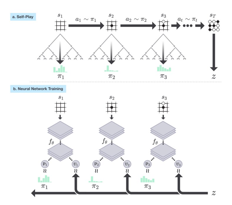
Figure 1: Self-play reinforcement learning in AlphaGo Zero. a The program plays a game $s_1, \ldots, s_T$ against itself. In each position $s_t$, a Monte-Carlo tree search (MCTS) $\alpha_\theta$ is executed (see Figure 2) using the latest neural network $f_\theta$. Moves are selected according to the search probabilities computed by the MCTS, $a_t \sim \pi_t$. The terminal position $s_T$ is scored according to the rules of the game to compute the game winner $z$. b Neural network training in AlphaGo Zero. The neural network takes the raw board position $s_t$ as its input, passes it through many convolutional layers with parameters $\theta$, and outputs both a vector $p_t$, representing a probability distribution over moves, and a scalar value $v_t$, representing the probability of the current player winning in position $s_t$. The neural network parameters $\theta$ are updated so as to maximise the similarity of the policy vector $p_t$ to the search probabilities $\pi_t$, and to minimise the error between the predicted winner $v_t$ and the game winner $z$ (see Equation 1). The new parameters are used in the next iteration of self-play a.

图 1：AlphaGo Zero 中的自我对弈强化学习。a 程序自己与自己下一局棋 $s_1, \ldots, s_T$。在每个局面 $s_t$，用最新的神经网络 $f_\theta$ 执行一次蒙特卡洛树搜索（MCTS）$\alpha_\theta$（见图 2）。着法按 MCTS 算出的搜索概率选取，$a_t \sim \pi_t$。终局 $s_T$ 按规则计分，得到胜者 $z$。b AlphaGo Zero 中的神经网络训练。网络把原始棋盘局面 $s_t$ 作为输入，经过许多带参数 $\theta$ 的卷积层，同时输出表示着法分布的向量 $p_t$，以及表示当前执棋方在 $s_t$ 获胜概率的标量 $v_t$。更新参数 $\theta$，使策略向量 $p_t$ 尽量接近搜索概率 $\pi_t$，并减小预测胜者 $v_t$ 与对局胜者 $z$ 之间的误差（见公式 1）。新参数用于下一轮自我对弈 a。

The Monte-Carlo tree search uses the neural network $f_\theta$ to guide its simulations (see Figure 2). Each edge $(s, a)$ in the search tree stores a prior probability $P(s, a)$, a visit count $N(s, a)$, and an action-value $Q(s, a)$. Each simulation starts from the root state and iteratively selects moves that maximise an upper confidence bound $Q(s, a) + U(s, a)$, where $U(s, a) \propto P(s, a)/(1 + N(s, a))$, until a leaf node $s'$ is encountered. This leaf position is expanded and evaluated just once by the network to generate both prior probabilities and evaluation, $(P(s', \cdot), V(s')) = f_\theta(s')$. Each edge $(s, a)$ traversed in the simulation is updated to increment its visit count $N(s, a)$, and to update its action-value to the mean evaluation over these simulations, $Q(s, a) = \frac{1}{N(s, a)} \sum_{s'|s,a \rightarrow s'} V(s')$, where $s, a \rightarrow s'$ indicates that a simulation eventually reached $s'$ after taking move $a$ from position $s$.

蒙特卡洛树搜索用神经网络 $f_\theta$ 引导模拟（见图 2）。搜索树的每条边 $(s, a)$ 保存先验概率 $P(s, a)$、访问次数 $N(s, a)$ 和动作价值 $Q(s, a)$。每次模拟从根节点出发，迭代选择使上置信界 $Q(s, a) + U(s, a)$ 最大的着法，其中 $U(s, a) \propto P(s, a)/(1 + N(s, a))$，直到遇到叶节点 $s'$。这个叶子局面只被网络评估一次，同时给出先验概率和评估，$(P(s', \cdot), V(s')) = f_\theta(s')$。模拟中经过的每条边 $(s, a)$ 都会增加访问次数 $N(s, a)$，并把动作价值更新为这些模拟评估的均值 $Q(s, a) = \frac{1}{N(s, a)} \sum_{s'|s,a \rightarrow s'} V(s')$，其中 $s, a \rightarrow s'$ 表示一次模拟在局面 $s$ 走出 $a$ 之后最终到达了 $s'$。

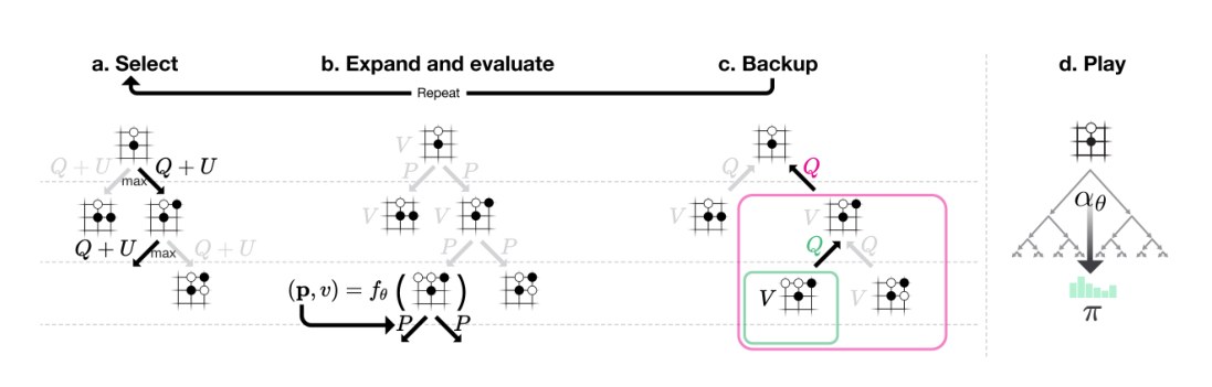
Figure 2: Monte-Carlo tree search in AlphaGo Zero. a Each simulation traverses the tree by selecting the edge with maximum action-value $Q$, plus an upper confidence bound $U$ that depends on a stored prior probability $P$ and visit count $N$ for that edge (which is incremented once traversed). b The leaf node is expanded and the associated position $s$ is evaluated by the neural network $(P(s, \cdot), V(s)) = f_\theta(s)$; the vector of $P$ values are stored in the outgoing edges from $s$. c Action-values $Q$ are updated to track the mean of all evaluations $V$ in the subtree below that action. d Once the search is complete, search probabilities $\pi$ are returned, proportional to $N^{1/\tau}$, where $N$ is the visit count of each move from the root state and $\tau$ is a parameter controlling temperature.

图 2：AlphaGo Zero 中的蒙特卡洛树搜索。a 每次模拟沿树下行，选择动作价值 $Q$ 加上置信上界 $U$ 最大的边；$U$ 取决于该边保存的先验概率 $P$ 和访问次数 $N$（经过时递增）。b 扩展叶节点，并用神经网络评估对应局面 $s$，得到 $(P(s, \cdot), V(s)) = f_\theta(s)$；$P$ 向量存入 $s$ 的出边。c 动作价值 $Q$ 更新为该动作子树中所有评估 $V$ 的均值。d 搜索结束后返回搜索概率 $\pi$，与 $N^{1/\tau}$ 成正比，其中 $N$ 是根节点各着法的访问次数，$\tau$ 是控制温度的参数。

MCTS may be viewed as a self-play algorithm that, given neural network parameters $\theta$ and a root position $s$, computes a vector of search probabilities recommending moves to play, $\pi = \alpha_\theta(s)$, proportional to the exponentiated visit count for each move, $\pi_a \propto N(s, a)^{1/\tau}$, where $\tau$ is a temperature parameter.

MCTS 也可以看成一种自我对弈算法：给定网络参数 $\theta$ 和根局面 $s$，它算出一个推荐着法的搜索概率向量 $\pi = \alpha_\theta(s)$，与各着法访问次数的幂次成正比，$\pi_a \propto N(s, a)^{1/\tau}$，其中 $\tau$ 是温度参数。

The neural network is trained by a self-play reinforcement learning algorithm that uses MCTS to play each move. First, the neural network is initialised to random weights $\theta_0$. At each subsequent iteration $i \ge 1$, games of self-play are generated (Figure 1a). At each time-step $t$, an MCTS search $\pi_t = \alpha_{\theta_{i-1}}(s_t)$ is executed using the previous iteration of neural network $f_{\theta_{i-1}}$, and a move is played by sampling the search probabilities $\pi_t$. A game terminates at step $T$ when both players pass, when the search value drops below a resignation threshold, or when the game exceeds a maximum length; the game is then scored to give a final reward of $r_T \in \{-1, +1\}$ (see Methods for details). The data for each time-step $t$ is stored as $(s_t, \pi_t, z_t)$ where $z_t = \pm r_T$ is the game winner from the perspective of the current player at step $t$. In parallel (Figure 1b), new network parameters $\theta_i$ are trained from data $(s, \pi, z)$ sampled uniformly among all time-steps of the last iteration(s) of self-play. The neural network $(p, v) = f_{\theta_i}(s)$ is adjusted to minimise the error between the predicted value $v$ and the self-play winner $z$, and to maximise the similarity of the neural network move probabilities $p$ to the search probabilities $\pi$. Specifically, the parameters $\theta$ are adjusted by gradient descent on a loss function $l$ that sums over mean-squared error and cross-entropy losses respectively,

神经网络由一种用 MCTS 走出每一步的自我对弈强化学习算法来训练。网络先初始化为随机权重 $\theta_0$。之后每次迭代 $i \ge 1$，都会生成自我对弈棋局（图 1a）。在每个时刻 $t$，用上一轮网络 $f_{\theta_{i-1}}$ 执行一次 MCTS 搜索 $\pi_t = \alpha_{\theta_{i-1}}(s_t)$，再按搜索概率 $\pi_t$ 采样走出一步。对局在第 $T$ 步结束：双方都停着、搜索价值低于认输阈值，或对局超过最大长度；随后计分，给出终局奖励 $r_T \in \{-1, +1\}$（细节见 Methods）。每个时刻 $t$ 的数据存为 $(s_t, \pi_t, z_t)$，其中 $z_t = \pm r_T$ 是从该时刻执棋方视角看到的胜者。与此并行（图 1b），新参数 $\theta_i$ 从最近一轮或几轮自我对弈所有时刻中均匀抽样的数据 $(s, \pi, z)$ 上训练。网络 $(p, v) = f_{\theta_i}(s)$ 被调整，以减小预测价值 $v$ 与自我对弈胜者 $z$ 之间的误差，并增大网络着法概率 $p$ 与搜索概率 $\pi$ 的相似度。具体来说，参数 $\theta$ 对同时包含均方误差和交叉熵的损失函数 $l$ 做梯度下降，

$$(p, v) = f_{\theta}(s), \qquad l = (z - v)^{2} - \pi^{\top} \log p + c\|\theta\|^{2} \tag{1}$$

where $c$ is a parameter controlling the level of $L_2$ weight regularisation (to prevent overfitting).

其中 $c$ 是控制 $L_2$ 权重正则强度的参数（用来防止过拟合）。

Empirical Analysis of AlphaGo Zero Training

AlphaGo Zero 训练的实证分析

We applied our reinforcement learning pipeline to train our program AlphaGo Zero. Training started from completely random behaviour and continued without human intervention for approximately 3 days. Over the course of training, 4.9 million games of self-play were generated, using 1,600 simulations for each MCTS, which corresponds to approximately 0.4s thinking time per move. Parameters were updated from 700,000 mini-batches of 2,048 positions. The neural network contained 20 residual blocks (see Methods for further details).

我们用这条强化学习流水线训练了程序 AlphaGo Zero。训练从完全随机的行为起步，在没有人工干预的情况下持续大约 3 天。训练过程中生成了 490 万局自我对弈，每次 MCTS 使用 1,600 次模拟，大约相当于每步思考 0.4 秒。参数由 70 万个大小为 2,048 个局面的小批量更新。神经网络包含 20 个残差块（更多细节见 Methods）。

Figure 3a shows the performance of AlphaGo Zero during self-play reinforcement learning, as a function of training time, on an Elo scale. Learning progressed smoothly throughout training, and did not suffer from the oscillations or catastrophic forgetting suggested in prior literature. Surprisingly, AlphaGo Zero outperformed AlphaGo Lee after just 36 hours; for comparison, AlphaGo Lee was trained over several months. After 72 hours, we evaluated AlphaGo Zero against the exact version of AlphaGo Lee that defeated Lee Sedol, under the 2 hour time controls and match conditions as were used in the man-machine match in Seoul (see Methods). AlphaGo Zero used a single machine with 4 Tensor Processing Units (TPUs), while AlphaGo Lee was distributed over many machines and used 48 TPUs. AlphaGo Zero defeated AlphaGo Lee by 100 games to 0 (see Extended Data Figure 5 and Supplementary Information).

图 3a 按 Elo 标尺给出 AlphaGo Zero 在自我对弈强化学习中随训练时间变化的表现。整个训练过程学习曲线平滑，并没有出现文献中提到的振荡或灾难性遗忘。出人意料的是，AlphaGo Zero 只用 36 小时就超过了 AlphaGo Lee；作为对照，AlphaGo Lee 的训练持续了几个月。72 小时之后，我们让 AlphaGo Zero 对阵击败 Lee Sedol 的那个精确版本的 AlphaGo Lee，用时和比赛条件与首尔人机大战相同（见 Methods）：每方 2 小时。AlphaGo Zero 跑在一台配有 4 块张量处理单元（TPU）的机器上，而 AlphaGo Lee 分布在多台机器上、使用 48 块 TPU。AlphaGo Zero 以 100 局全胜击败 AlphaGo Lee（见扩展数据图 5 和补充材料）。

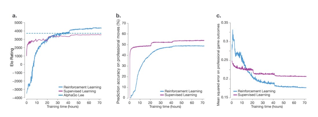
Figure 3: Empirical evaluation of AlphaGo Zero. a Performance of self-play reinforcement learning. The plot shows the performance of each MCTS player $\alpha_{\theta_i}$ from each iteration $i$ of reinforcement learning in AlphaGo Zero. Elo ratings were computed from evaluation games between different players, using 0.4 seconds of thinking time per move (see Methods). For comparison, a similar player trained by supervised learning from human data, using the KGS data-set, is also shown. b Prediction accuracy on human professional moves. The plot shows the accuracy of the neural network $f_{\theta_i}$, at each iteration of self-play $i$, in predicting human professional moves from the GoKifu data-set. The accuracy measures the percentage of positions in which the neural network assigns the highest probability to the human move. The accuracy of a neural network trained by supervised learning is also shown. c Mean-squared error (MSE) on human professional game outcomes. The plot shows the MSE of the neural network $f_{\theta_i}$, at each iteration of self-play $i$, in predicting the outcome of human professional games from the GoKifu data-set. The MSE is between the actual outcome $z \in \{-1, +1\}$ and the neural network value $v$, scaled by a factor of $1/4$ to the range $[0, 1]$. The MSE of a neural network trained by supervised learning is also shown.

图 3：AlphaGo Zero 的实证评估。a 自我对弈强化学习的表现。图中给出强化学习每次迭代 $i$ 对应的 MCTS 棋手 $\alpha_{\theta_i}$ 的表现。Elo 等级分由不同棋手之间的评估对局计算，每步思考 0.4 秒（见 Methods）。作为对照，图中也画出了一个用 KGS 数据集、从人类数据做监督学习训练的类似棋手。b 预测人类职业棋手着法的准确率。图中给出每次自我对弈迭代 $i$ 的网络 $f_{\theta_i}$ 在 GoKifu 数据集上预测人类职业着法的准确率。准确率定义为网络把最高概率赋给人类着法的局面所占比例。图中也画出了监督学习训练的网络的准确率。c 对人类职业对局结果的均方误差（MSE）。图中给出每次迭代 $i$ 的网络 $f_{\theta_i}$ 在 GoKifu 数据集上预测人类职业对局结果的 MSE。MSE 计算的是真实结果 $z \in \{-1, +1\}$ 与网络价值 $v$ 之间的误差，并乘以 $1/4$ 缩放到 $[0, 1]$。图中也画出了监督学习网络的 MSE。

To assess the merits of self-play reinforcement learning, compared to learning from human data, we trained a second neural network (using the same architecture) to predict expert moves in the KGS data-set; this achieved state-of-the-art prediction accuracy compared to prior work (see Extended Data Table 1 and 2 respectively). Supervised learning achieved better initial performance, and was better at predicting the outcome of human professional games (Figure 3). Notably, although supervised learning achieved higher move prediction accuracy, the self-learned player performed much better overall, defeating the human-trained player within the first 24 hours of training. This suggests that AlphaGo Zero may be learning a strategy that is qualitatively different to human play.

为了比较自我对弈强化学习与从人类数据学习的优劣，我们用同一套结构训练了第二个神经网络，用来预测 KGS 数据集中的高手着法；其预测准确率优于先前工作（分别见扩展数据表 1 和表 2）。监督学习起步更快，也更擅长预测人类职业对局的胜负（图 3）。值得注意的是，尽管监督学习的着法预测准确率更高，自我学成的棋手整体表现却好得多，并在训练的前 24 小时内就击败了用人类数据训练的棋手。这说明 AlphaGo Zero 学到的策略，在性质上可能与人类棋风不同。

To separate the contributions of architecture and algorithm, we compared the performance of the neural network architecture in AlphaGo Zero with the previous neural network architecture used in AlphaGo Lee (see Figure 4). Four neural networks were created, using either separate policy and value networks, as in AlphaGo Lee, or combined policy and value networks, as in AlphaGo Zero; and using either the convolutional network architecture from AlphaGo Lee or the residual network architecture from AlphaGo Zero. Each network was trained to minimise the same loss function (Equation 1) using a fixed data-set of self-play games generated by AlphaGo Zero after 72 hours of self-play training. Using a residual network was more accurate, achieved lower error, and improved performance in AlphaGo by over 600 Elo. Combining policy and value together into a single network slightly reduced the move prediction accuracy, but reduced the value error and boosted playing performance in AlphaGo by around another 600 Elo. This is partly due to improved computational efficiency, but more importantly the dual objective regularises the network to a common representation that supports multiple use cases.

为了把结构贡献和算法贡献分开，我们比较了 AlphaGo Zero 的网络结构与 AlphaGo Lee 此前使用的网络结构（见图 4）。一共训练了四个网络：策略网络与价值网络可以像 AlphaGo Lee 那样分开，也可以像 AlphaGo Zero 那样合并；卷积结构则可以采用 AlphaGo Lee 的普通卷积，或 AlphaGo Zero 的残差网络。每个网络都在同一损失函数（公式 1）上训练，数据是 AlphaGo Zero 自我对弈 72 小时后生成的固定自我对弈棋谱。使用残差网络更准确、误差更低，并使 AlphaGo 的棋力提高超过 600 Elo。把策略和价值合并进同一个网络，会略微降低着法预测准确率，但减小了价值误差，并使棋力再提高大约 600 Elo。这部分来自计算效率的提升，更重要的是双重目标把网络正则到一套能同时服务多种用途的公共表示上。

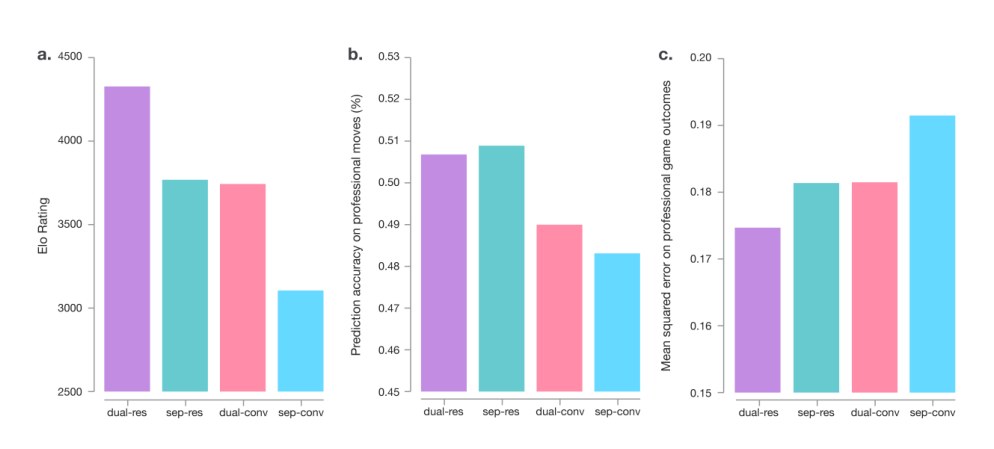
Figure 4: Comparison of neural network architectures in AlphaGo Zero and AlphaGo Lee. Comparison of neural network architectures using either separate ("sep") or combined policy and value networks ("dual"), and using either convolutional ("conv") or residual networks ("res"). The combinations "dual-res" and "sep-conv" correspond to the neural network architectures used in AlphaGo Zero and AlphaGo Lee respectively. Each network was trained on a fixed data-set generated by a previous run of AlphaGo Zero. a Each trained network was combined with AlphaGo Zero's search to obtain a different player. Elo ratings were computed from evaluation games between these different players, using 5 seconds of thinking time per move. b Prediction accuracy on human professional moves (from the GoKifu data-set) for each network architecture. c Mean-squared error on human professional game outcomes (from the GoKifu data-set) for each network architecture.

图 4：AlphaGo Zero 与 AlphaGo Lee 的神经网络结构比较。比较时分别采用分开（"sep"）或合并（"dual"）的策略与价值网络，以及普通卷积（"conv"）或残差网络（"res"）。组合 "dual-res" 和 "sep-conv" 分别对应 AlphaGo Zero 和 AlphaGo Lee 使用的网络结构。每个网络都在先前一次 AlphaGo Zero 运行生成的固定数据集上训练。a 每个训练好的网络都与 AlphaGo Zero 的搜索结合，得到不同的棋手。Elo 等级分由这些棋手之间的评估对局计算，每步思考 5 秒。b 各网络结构在人类职业着法（GoKifu 数据集）上的预测准确率。c 各网络结构在人类职业对局结果（GoKifu 数据集）上的均方误差。

Knowledge Learned by AlphaGo Zero

AlphaGo Zero 学到的围棋知识

AlphaGo Zero discovered a remarkable level of Go knowledge during its self-play training process. This included fundamental elements of human Go knowledge, and also non-standard strategies beyond the scope of traditional Go knowledge.

在自我对弈训练过程中，AlphaGo Zero 发现了相当丰富的围棋知识。其中既包括人类围棋知识的基本要素，也有超出传统围棋知识范围的非标准策略。

Figure 5 shows a timeline indicating when professional joseki (corner sequences) were discovered (Figure 5a, Extended Data Figure 1); ultimately AlphaGo Zero preferred new joseki variants that were previously unknown (Figure 5b, Extended Data Figure 2). Figure 5c and the Supplementary Information show several fast self-play games played at different stages of training. Tournament length games played at regular intervals throughout training are shown in Extended Data Figure 3 and Supplementary Information. AlphaGo Zero rapidly progressed from entirely random moves towards a sophisticated understanding of Go concepts including fuseki (opening), tesuji (tactics), life-and-death, ko (repeated board situations), yose (endgame), capturing races, sente (initiative), shape, influence and territory, all discovered from first principles. Surprisingly, shicho ("ladder" capture sequences that may span the whole board) — one of the first elements of Go knowledge learned by humans — were only understood by AlphaGo Zero much later in training.

图 5 用时间线标出职业定式（角部变化）被发现的时间（图 5a，扩展数据图 1）；最终 AlphaGo Zero 更偏好此前不为人知的新定式变体（图 5b，扩展数据图 2）。图 5c 和补充材料给出了训练不同阶段的若干快速自我对弈对局。训练过程中定期进行的比赛时长对局见扩展数据图 3 和补充材料。AlphaGo Zero 很快从完全随机的着法，发展到对布局（fuseki）、手筋（tesuji）、死活、劫（重复出现的棋形）、官子（yose）、对杀、先手（sente）、棋形、厚势和实地等概念有细致理解，而且都是从第一性原理中自己发现的。出人意料的是，征子（可能贯穿全盘的“梯子”吃子）——人类最早学会的围棋知识之一——直到训练相当晚的阶段才被 AlphaGo Zero 理解。

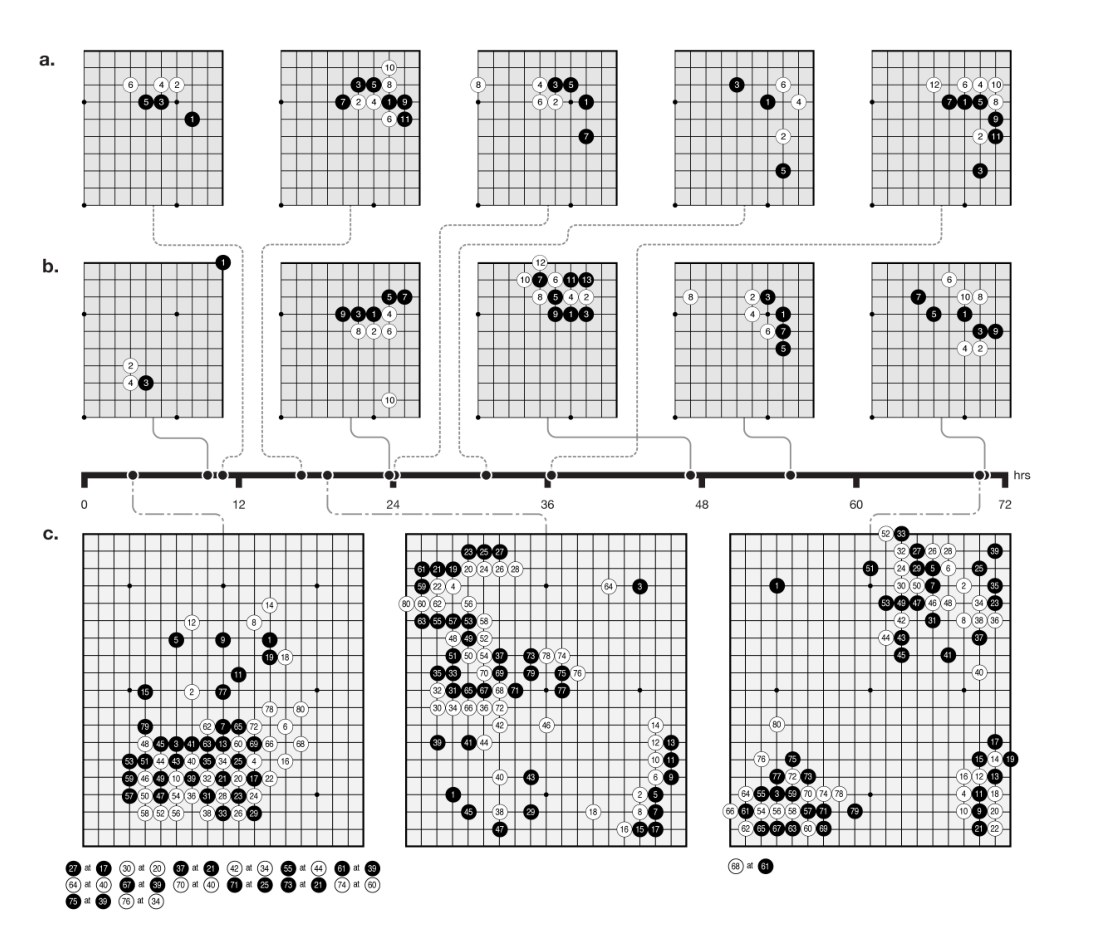
Figure 5: Go knowledge learned by AlphaGo Zero. a Five human joseki (common corner sequences) discovered during AlphaGo Zero training. The associated timestamps indicate the first time each sequence occurred (taking account of rotation and reflection) during self-play training. Extended Data Figure 1 provides the frequency of occurrence over training for each sequence. b Five joseki favoured at different stages of self-play training. Each displayed corner sequence was played with the greatest frequency, among all corner sequences, during an iteration of self-play training. The timestamp of that iteration is indicated on the timeline. At 10 hours a weak corner move was preferred. At 47 hours the 3-3 invasion was most frequently played. This joseki is also common in human professional play; however AlphaGo Zero later discovered and preferred a new variation. Extended Data Figure 2 provides the frequency of occurrence over time for all five sequences and the new variation. c The first 80 moves of three self-play games that were played at different stages of training, using 1,600 simulations (around 0.4s) per search. At 3 hours, the game focuses greedily on capturing stones, much like a human beginner. At 19 hours, the game exhibits the fundamentals of life-and-death, influence and territory. At 70 hours, the game is beautifully balanced, involving multiple battles and a complicated ko fight, eventually resolving into a half-point win for white. See Supplementary Information for the full games.

图 5：AlphaGo Zero 学到的围棋知识。a 训练过程中发现的五种人类定式（常见角部变化）。时间戳标出每种变化在自我对弈训练中首次出现的时刻（已考虑旋转和镜像）。扩展数据图 1 给出每种变化在训练中出现的频率。b 自我对弈训练不同阶段最受偏爱的五种定式。图中展示的每种角部变化，都是某次自我对弈迭代中在所有角部变化里出现频率最高的。该次迭代的时间标在时间线上。10 小时时，程序偏好一种较弱的角部着法。47 小时时，最常下的是三三入侵。这一套定式在人类职业对局中也很常见；不过 AlphaGo Zero 后来发现并更偏好一种新变化。扩展数据图 2 给出全部五种变化以及新变体随时间的出现频率。c 训练不同阶段三局自我对弈的前 80 手，每次搜索使用 1,600 次模拟（大约 0.4 秒）。3 小时时，对局贪婪地忙于吃子，很像人类初学者。19 小时时，棋已经具备死活、厚势和实地的基本要素。70 小时时，对局极为均衡，包含多处战斗和复杂的劫争，最终白棋以半目获胜。完整对局见补充材料。

Final Performance of AlphaGo Zero

AlphaGo Zero 的最终表现

We subsequently applied our reinforcement learning pipeline to a second instance of AlphaGo Zero using a larger neural network and over a longer duration. Training again started from completely random behaviour and continued for approximately 40 days. Over the course of training, 29 million games of self-play were generated. Parameters were updated from 3.1 million mini-batches of 2,048 positions each. The neural network contained 40 residual blocks. The learning curve is shown in Figure 6a. Games played at regular intervals throughout training are shown in Extended Data Figure 4 and Supplementary Information.

随后，我们把同一条强化学习流水线用到第二个 AlphaGo Zero 实例上，网络更大、训练时间也更长。训练再次从完全随机的行为起步，持续大约 40 天。训练过程中生成了 2900 万局自我对弈。参数由 310 万个大小为 2,048 个局面的小批量更新。神经网络包含 40 个残差块。学习曲线见图 6a。训练过程中定期进行的对局见扩展数据图 4 和补充材料。

We evaluated the fully trained AlphaGo Zero using an internal tournament against AlphaGo Fan, AlphaGo Lee, and several previous Go programs. We also played games against the strongest existing program, AlphaGo Master — a program based on the algorithm and architecture presented in this paper but utilising human data and features (see Methods) — which defeated the strongest human professional players 60–0 in online games in January 2017. In our evaluation, all programs were allowed 5 seconds of thinking time per move; AlphaGo Zero and AlphaGo Master each played on a single machine with 4 TPUs; AlphaGo Fan and AlphaGo Lee were distributed over 176 GPUs and 48 TPUs respectively. We also included a player based solely on the raw neural network of AlphaGo Zero; this player simply selected the move with maximum probability.

我们用内部循环赛评估训练完成的 AlphaGo Zero，对手包括 AlphaGo Fan、AlphaGo Lee 以及若干此前的围棋程序。我们也对阵了当时最强的程序 AlphaGo Master——它基于本文给出的算法和结构，但仍使用人类数据和特征（见 Methods）——该程序曾在 2017 年 1 月的网上对局中以 60 比 0 击败最强的人类职业棋手。评估中，所有程序每步有 5 秒思考时间；AlphaGo Zero 和 AlphaGo Master 各自跑在一台配有 4 块 TPU 的机器上；AlphaGo Fan 和 AlphaGo Lee 则分别分布在 176 块 GPU 和 48 块 TPU 上。我们还加入了一个只使用 AlphaGo Zero 原始神经网络的棋手：它直接选择概率最大的着法。

Figure 6b shows the performance of each program on an Elo scale. The raw neural network, without using any lookahead, achieved an Elo rating of 3,055. AlphaGo Zero achieved a rating of 5,185, compared to 4,858 for AlphaGo Master, 3,739 for AlphaGo Lee and 3,144 for AlphaGo Fan. Finally, we evaluated AlphaGo Zero head to head against AlphaGo Master in a 100 game match with 2 hour time controls. AlphaGo Zero won by 89 games to 11 (see Extended Data Figure 6 and Supplementary Information).

图 6b 按 Elo 标尺给出各程序的表现。不做任何前瞻、只靠原始神经网络的棋手，Elo 等级分为 3,055。AlphaGo Zero 达到 5,185，相较之下 AlphaGo Master 为 4,858，AlphaGo Lee 为 3,739，AlphaGo Fan 为 3,144。最后，我们让 AlphaGo Zero 与 AlphaGo Master 进行 100 局、每方 2 小时的对决。AlphaGo Zero 以 89 比 11 获胜（见扩展数据图 6 和补充材料）。

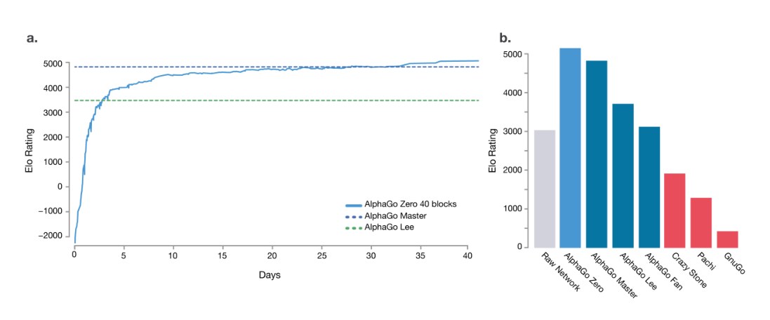
Figure 6: Performance of AlphaGo Zero. a Learning curve for AlphaGo Zero using larger 40 block residual network over 40 days. The plot shows the performance of each player $\alpha_{\theta_i}$ from each iteration $i$ of our reinforcement learning algorithm. Elo ratings were computed from evaluation games between different players, using 0.4 seconds per search (see Methods). b Final performance of AlphaGo Zero. AlphaGo Zero was trained for 40 days using a 40 residual block neural network. The plot shows the results of a tournament between: AlphaGo Zero, AlphaGo Master (defeated top human professionals 60-0 in online games), AlphaGo Lee (defeated Lee Sedol), AlphaGo Fan (defeated Fan Hui), as well as previous Go programs Crazy Stone, Pachi and GnuGo. Each program was given 5 seconds of thinking time per move. AlphaGo Zero and AlphaGo Master played on a single machine on the Google Cloud; AlphaGo Fan and AlphaGo Lee were distributed over many machines. The raw neural network from AlphaGo Zero is also included, which directly selects the move $a$ with maximum probability $p_a$, without using MCTS. Programs were evaluated on an Elo scale: a 200 point gap corresponds to a 75% probability of winning.

图 6：AlphaGo Zero 的表现。a 使用更大的 40 块残差网络、训练 40 天的 AlphaGo Zero 学习曲线。图中给出强化学习算法每次迭代 $i$ 对应棋手 $\alpha_{\theta_i}$ 的表现。Elo 等级分由不同棋手之间的评估对局计算，每次搜索 0.4 秒（见 Methods）。b AlphaGo Zero 的最终表现。AlphaGo Zero 使用 40 个残差块的网络训练了 40 天。图中给出循环赛结果，参赛者包括：AlphaGo Zero、AlphaGo Master（曾在网上对局中以 60 比 0 击败顶尖职业棋手）、AlphaGo Lee（击败 Lee Sedol）、AlphaGo Fan（击败 Fan Hui），以及此前的围棋程序 Crazy Stone、Pachi 和 GnuGo。每个程序每步有 5 秒思考时间。AlphaGo Zero 和 AlphaGo Master 跑在 Google Cloud 的单机上；AlphaGo Fan 和 AlphaGo Lee 分布在多台机器上。图中也包括 AlphaGo Zero 的原始神经网络，它不使用 MCTS，直接选择概率 $p_a$ 最大的着法 $a$。程序按 Elo 标尺评估：200 分的差距对应大约 75% 的胜率。

Conclusion

结论

Our results comprehensively demonstrate that a pure reinforcement learning approach is fully feasible, even in the most challenging of domains: it is possible to train to superhuman level, without human examples or guidance, given no knowledge of the domain beyond basic rules. Furthermore, a pure reinforcement learning approach requires just a few more hours to train, and achieves much better asymptotic performance, compared to training on human expert data. Using this approach, AlphaGo Zero defeated the strongest previous versions of AlphaGo, which were trained from human data using handcrafted features, by a large margin.

我们的结果相当完整地表明，纯强化学习即使在最具挑战的领域也完全可行：在只知道基本规则、没有任何人类范例或指导的情况下，仍然可以训练到超人水平。而且，与在人类高手数据上训练相比，纯强化学习只需再多花几个小时，渐近表现却好得多。用这种方法，AlphaGo Zero 以很大优势击败了此前最强的、用人类数据和手工特征训练的各版 AlphaGo。

Humankind has accumulated Go knowledge from millions of games played over thousands of years, collectively distilled into patterns, proverbs and books. In the space of a few days, starting tabula rasa, AlphaGo Zero was able to rediscover much of this Go knowledge, as well as novel strategies that provide new insights into the oldest of games.

人类从数千年来数百万局棋中积累围棋知识，并把它们提炼成棋形、口诀和书籍。只用几天时间，从一张白纸出发，AlphaGo Zero 就重新发现了其中的大部分知识，还找到了能为这门最古老的博弈提供新见解的新策略。

Methods

Reinforcement learning

强化学习

Policy iteration is a classic algorithm that generates a sequence of improving policies, by alternating between policy evaluation — estimating the value function of the current policy — and policy improvement — using the current value function to generate a better policy. A simple approach to policy evaluation is to estimate the value function from the outcomes of sampled trajectories. A simple approach to policy improvement is to select actions greedily with respect to the value function. In large state spaces, approximations are necessary to evaluate each policy and to represent its improvement.

策略迭代是一种经典算法：它在策略评估——估计当前策略的价值函数——和策略改进——用当前价值函数生成更好的策略——之间交替，从而得到一系列逐渐变强的策略。一种简单的策略评估做法，是用采样轨迹的结果来估计价值函数。一种简单的策略改进做法，是相对价值函数贪婪地选择动作。在大型状态空间里，评估每个策略并表示它的改进都需要近似。

Classification-based reinforcement learning improves the policy using a simple Monte-Carlo search. Many rollouts are executed for each action; the action with the maximum mean value provides a positive training example, while all other actions provide negative training examples; a policy is then trained to classify actions as positive or negative, and used in subsequent rollouts. This may be viewed as a precursor to the policy component of AlphaGo Zero's training algorithm when $\tau \rightarrow 0$.

基于分类的强化学习用一次简单的蒙特卡洛搜索来改进策略。对每个动作执行多次走子；均值最大的动作作为正例，其余动作作为负例；再训练一个策略把动作分为正负两类，并用于后续走子。当 $\tau \rightarrow 0$ 时，这可以看成 AlphaGo Zero 训练算法中策略部分的前身。

A more recent instantiation, classification-based modified policy iteration (CBMPI), also performs policy evaluation by regressing a value function towards truncated rollout values, similar to the value component of AlphaGo Zero; this achieved state-of-the-art results in the game of Tetris. However, this prior work was limited to simple rollouts and linear function approximation using handcrafted features.

更新近的一个实例是基于分类的修正策略迭代（CBMPI），它还通过把价值函数回归到截断走子的价值上来做策略评估，这与 AlphaGo Zero 的价值部分相似；该方法在俄罗斯方块上取得了当时最好的结果。不过，这一先前工作仍局限于简单走子，以及使用手工特征的线性函数近似。

The AlphaGo Zero self-play algorithm can similarly be understood as an approximate policy iteration scheme in which MCTS is used for both policy improvement and policy evaluation. Policy improvement starts with a neural network policy, executes an MCTS based on that policy's recommendations, and then projects the (much stronger) search policy back into the function space of the neural network. Policy evaluation is applied to the (much stronger) search policy: the outcomes of self-play games are also projected back into the function space of the neural network. These projection steps are achieved by training the neural network parameters to match the search probabilities and self-play game outcome respectively.

AlphaGo Zero 的自我对弈算法同样可以理解成一种近似策略迭代：MCTS 同时用于策略改进和策略评估。策略改进从神经网络策略出发，基于该策略的建议执行一次 MCTS，再把（强得多的）搜索策略投影回神经网络的函数空间。策略评估则作用在（强得多的）搜索策略上：自我对弈的胜负结果同样被投影回神经网络的函数空间。这些投影步骤，是通过训练网络参数去拟合搜索概率和自我对弈结果来完成的。

Guo et al. also project the output of MCTS into a neural network, either by regressing a value network towards the search value, or by classifying the action selected by MCTS. This approach was used to train a neural network for playing Atari games; however, the MCTS was fixed — there was no policy iteration — and did not make any use of the trained networks.

Guo 等人同样把 MCTS 的输出投影进神经网络，做法要么是让价值网络回归搜索价值，要么是分类 MCTS 选出的动作。这一思路曾用来训练玩 Atari 游戏的神经网络；不过那里的 MCTS 是固定的——没有策略迭代——也没有使用训练得到的网络。

Self-play reinforcement learning in games

博弈中的自我对弈强化学习

Our approach is most directly applicable to zero-sum games of perfect information. We follow the formalism of alternating Markov games described in previous work, noting that algorithms based on value or policy iteration extend naturally to this setting.

我们的方法最直接适用于完全信息零和博弈。我们沿用先前工作中交替马尔可夫博弈的形式化，并指出基于价值或策略迭代的算法可以自然推广到这一设定。

Self-play reinforcement learning has previously been applied to the game of Go. NeuroGo used a neural network to represent a value function, using a sophisticated architecture based on Go knowledge regarding connectivity, territory and eyes. This neural network was trained by temporal-difference learning to predict territory in games of self-play, building on prior work. A related approach, RLGO, represented the value function instead by a linear combination of features, exhaustively enumerating all $3 \times 3$ patterns of stones; it was trained by temporal-difference learning to predict the winner in games of self-play. Both NeuroGo and RLGO achieved a weak amateur level of play.

自我对弈强化学习此前已经用于围棋。NeuroGo 用神经网络表示价值函数，结构相当精巧，并嵌入了关于连通、实地和眼位的围棋知识。该网络用时序差分学习，在自我对弈中预测实地，建立在更早工作之上。相关方法 RLGO 则用特征的线性组合表示价值函数，穷尽枚举所有 $3 \times 3$ 的棋子模式；它用时序差分学习预测自我对弈的胜者。NeuroGo 和 RLGO 都只达到较弱的业余水平。

Monte-Carlo tree search (MCTS) may also be viewed as a form of self-play reinforcement learning. The nodes of the search tree contain the value function for the positions encountered during search; these values are updated to predict the winner of simulated games of self-play. MCTS programs have previously achieved strong amateur level in Go, but used substantial domain expertise: a fast rollout policy, based on handcrafted features, that evaluates positions by running simulations until the end of the game; and a tree policy, also based on handcrafted features, that selects moves within the search tree.

蒙特卡洛树搜索（MCTS）也可以看成一种自我对弈强化学习。搜索树的节点保存搜索中遇到的局面的价值函数；这些价值被更新，用来预测模拟自我对弈的胜者。MCTS 程序此前已经在围棋中达到较强的业余水平，但用了不少领域专长：一种基于手工特征的快速走子策略，通过对局模拟到终局来评估局面；以及同样基于手工特征、在搜索树内选择着法的树策略。

Self-play reinforcement learning approaches have achieved high levels of performance in other games: chess, checkers, backgammon, othello, Scrabble and most recently poker. In all of these examples, a value function was trained by regression or temporal-difference learning from training data generated by self-play. The trained value function was used as an evaluation function in an alpha-beta search, a simple Monte-Carlo search, or counterfactual regret minimisation. However, these methods utilised handcrafted input features or handcrafted feature templates. In addition, the learning process used supervised learning to initialise weights, hand-selected weights for piece values, handcrafted restrictions on the action space, or used pre-existing computer programs as training opponents or to generate game records.

自我对弈强化学习在其他博弈中也达到了很高的水平：国际象棋、跳棋、西洋双陆、奥赛罗、Scrabble，以及最近的扑克。这些例子都是用回归或时序差分学习，从自我对弈产生的数据中训练价值函数。训练好的价值函数再作为评估函数，用于 alpha-beta 搜索、简单的蒙特卡洛搜索，或反事实后悔最小化。不过，这些方法使用了手工输入特征或手工特征模板。此外，学习过程还用监督学习初始化权重、手工选定棋子分值、手工限制动作空间，或者把已有计算机程序当作训练对手或用来生成棋谱。

Many of the most successful and widely used reinforcement learning methods were first introduced in the context of zero-sum games: temporal-difference learning was first introduced for a checkers-playing program, while MCTS was introduced for the game of Go. However, very similar algorithms have subsequently proven highly effective in video games, robotics, industrial control, and online recommendation systems.

许多最成功、也最常用的强化学习方法，最初都是在零和博弈里提出的：时序差分学习最早出现在一个跳棋程序中，MCTS 则是为围棋提出的。不过，非常相近的算法后来在电子游戏、机器人、工业控制和在线推荐系统中也非常有效。

AlphaGo versions

AlphaGo 的多个版本

We compare three distinct versions of AlphaGo (plus AlphaGo Zero, described in this paper):

我们比较 AlphaGo 的三个不同版本（再加上本文描述的 AlphaGo Zero）：

1. AlphaGo Fan is the previously published program that played against Fan Hui in October 2015. This program was distributed over many machines using 176 GPUs.

1. AlphaGo Fan 是此前发表、于 2015 年 10 月对阵 Fan Hui 的程序。该程序分布在多台机器上，使用 176 块 GPU。

2. AlphaGo Lee is the program that defeated Lee Sedol 4–1 in March, 2016. It was previously unpublished but is similar in most regards to AlphaGo Fan. However, we highlight several key differences to facilitate a fair comparison. First, the value network was trained from the outcomes of fast games of self-play by AlphaGo, rather than games of self-play by the policy network; this procedure was iterated several times — an initial step towards the tabula rasa algorithm presented in this paper. Second, the policy and value networks were larger than those described in the original paper — using 12 convolutional layers of 256 planes respectively — and were trained for more iterations. This player was also distributed over many machines using 48 TPUs, rather than GPUs, enabling it to evaluate neural networks faster during search.

2. AlphaGo Lee 是 2016 年 3 月以 4 比 1 击败 Lee Sedol 的程序。它此前并未发表，在多数方面与 AlphaGo Fan 相近。不过，为便于公平比较，我们指出几处关键差异。第一，价值网络是从 AlphaGo 的快速自我对弈结果中训练的，而不是从策略网络的自我对弈中训练；这一流程迭代了多次——已经朝着本文提出的白纸算法迈出了第一步。第二，策略网络和价值网络都比原论文描述的更大——各使用 12 层、每层 256 个平面的卷积——并且训练了更多轮。这个棋手同样分布在多台机器上，使用 48 块 TPU 而不是 GPU，从而能在搜索中更快地评估神经网络。

3. AlphaGo Master is the program that defeated top human players by 60–0 in January, 2017. It was previously unpublished but uses the same neural network architecture, reinforcement learning algorithm, and MCTS algorithm as described in this paper. However, it uses the same handcrafted features and rollouts as AlphaGo Lee and training was initialised by supervised learning from human data.

3. AlphaGo Master 是 2017 年 1 月以 60 比 0 击败顶尖人类棋手的程序。它此前并未发表，但使用了本文描述的同一套神经网络结构、强化学习算法和 MCTS 算法。不过，它沿用了 AlphaGo Lee 的手工特征和走子，并且训练由人类数据上的监督学习初始化。

4. AlphaGo Zero is the program described in this paper. It learns from self-play reinforcement learning, starting from random initial weights, without using rollouts, with no human supervision, and using only the raw board history as input features. It uses just a single machine in the Google Cloud with 4 TPUs (AlphaGo Zero could also be distributed but we chose to use the simplest possible search algorithm).

4. AlphaGo Zero 就是本文描述的程序。它从随机初始权重出发，通过自我对弈强化学习来学习，不使用走子，没有人类监督，输入特征只用原始棋盘历史。它只使用 Google Cloud 上配有 4 块 TPU 的单机（AlphaGo Zero 也可以分布式运行，但我们选择了尽可能简单的搜索算法）。

Domain Knowledge

领域知识

Our primary contribution is to demonstrate that superhuman performance can be achieved without human domain knowledge. To clarify this contribution, we enumerate the domain knowledge that AlphaGo Zero uses, explicitly or implicitly, either in its training procedure or its Monte-Carlo tree search; these are the items of knowledge that would need to be replaced for AlphaGo Zero to learn a different (alternating Markov) game.

我们的主要贡献，是表明不借助人类领域知识也可以达到超人水平。为把这一点说清楚，我们列举 AlphaGo Zero 在训练流程或蒙特卡洛树搜索中显式或隐式使用的领域知识；若要让 AlphaGo Zero 学习另一种（交替马尔可夫）博弈，就需要替换这些知识条目。

1. AlphaGo Zero is provided with perfect knowledge of the game rules. These are used during MCTS, to simulate the positions resulting from a sequence of moves, and to score any simulations that reach a terminal state. Games terminate when both players pass, or after $19 \cdot 19 \cdot 2 = 722$ moves. In addition, the player is provided with the set of legal moves in each position.

1. AlphaGo Zero 被给予关于规则的完备知识。这些规则在 MCTS 中用来模拟一串着法之后的局面，并对到达终局的模拟计分。对局在双方都停着，或走满 $19 \cdot 19 \cdot 2 = 722$ 手时结束。此外，棋手在每个局面都会得到合法着法集合。

2. AlphaGo Zero uses Tromp-Taylor scoring during MCTS simulations and self-play training. This is because human scores (Chinese, Japanese or Korean rules) are not well-defined if the game terminates before territorial boundaries are resolved. However, all tournament and evaluation games were scored using Chinese rules.

2. 在 MCTS 模拟和自我对弈训练中，AlphaGo Zero 使用 Tromp-Taylor 计分。这是因为如果对局在地界尚未闭合时结束，人类使用的计分（中国、日本或韩国规则）并不良定义。不过，所有循环赛和评估对局都按中国规则计分。

3. The input features describing the position are structured as a $19 \times 19$ image; i.e. the neural network architecture is matched to the grid-structure of the board.

3. 描述局面的输入特征被组织成 $19 \times 19$ 的图像；也就是说，神经网络结构与棋盘的网格结构相匹配。

4. The rules of Go are invariant under rotation and reflection; this knowledge has been utilised in AlphaGo Zero both by augmenting the data set during training to include rotations and reflections of each position, and to sample random rotations or reflections of the position during MCTS (see Search Algorithm). Aside from komi, the rules of Go are also invariant to colour transposition; this knowledge is exploited by representing the board from the perspective of the current player (see Neural network architecture).

4. 围棋规则在旋转和镜像下不变；AlphaGo Zero 利用了这一点：训练时把每个局面的旋转和镜像加入数据集，并在 MCTS 中对局面随机采样旋转或镜像（见搜索算法）。除贴目外，围棋规则对黑白对调也保持不变；这一点通过从当前执棋方的视角表示棋盘来利用（见神经网络结构）。

AlphaGo Zero does not use any form of domain knowledge beyond the points listed above. It only uses its deep neural network to evaluate leaf nodes and to select moves (see section below). It does not use any rollout policy or tree policy, and the MCTS is not augmented by any other heuristics or domain-specific rules. No legal moves are excluded — even those filling in the player's own eyes (a standard heuristic used in all previous programs).

除上面列出的几点外，AlphaGo Zero 不再使用任何形式的领域知识。它只用深度神经网络评估叶节点并选择着法（见下一节）。它不使用任何走子策略或树策略，MCTS 也没有附加其他启发式或领域特定规则。任何合法着法都不会被排除——包括填自己的眼（这是此前所有程序都使用的标准启发式）。

The algorithm was started with random initial parameters for the neural network. The neural network architecture (see Neural Network Architecture) is based on the current state of the art in image recognition, and hyperparameters for training were chosen accordingly (see Self-Play Training Pipeline). MCTS search parameters were selected by Gaussian process optimisation, so as to optimise self-play performance of AlphaGo Zero using a neural network trained in a preliminary run. For the larger run (40 block, 40 days), MCTS search parameters were re-optimised using the neural network trained in the smaller run (20 block, 3 days). The training algorithm was executed autonomously without human intervention.

算法从神经网络的随机初始参数起步。网络结构（见神经网络结构）基于当时图像识别的先进做法，训练超参数也据此选定（见自我对弈训练流水线）。MCTS 搜索参数由高斯过程优化选定，目标是优化一次预实验中训练出的网络所对应的 AlphaGo Zero 自我对弈表现。在更大规模的运行（40 个残差块，40 天）中，搜索参数用较小规模运行（20 个残差块，3 天）训练出的网络重新优化。训练算法自动执行，没有人工干预。

Self-Play Training Pipeline

自我对弈训练流水线

AlphaGo Zero's self-play training pipeline consists of three main components, all executed asynchronously in parallel. Neural network parameters $\theta_i$ are continually optimised from recent self-play data; AlphaGo Zero players $\alpha_{\theta_i}$ are continually evaluated; and the best performing player so far, $\alpha_{\theta^*}$, is used to generate new self-play data.

AlphaGo Zero 的自我对弈训练流水线由三个主要部分组成，它们异步并行执行。神经网络参数 $\theta_i$ 持续用最近的自我对弈数据优化；AlphaGo Zero 棋手 $\alpha_{\theta_i}$ 持续接受评估；迄今表现最好的棋手 $\alpha_{\theta^*}$ 则用来生成新的自我对弈数据。

Optimisation

优化

Each neural network $f_{\theta_i}$ is optimised on the Google Cloud using TensorFlow, with 64 GPU workers and 19 CPU parameter servers. The batch-size is 32 per worker, for a total mini-batch size of 2,048. Each mini-batch of data is sampled uniformly at random from all positions from the most recent 500,000 games of self-play. Neural network parameters are optimised by stochastic gradient descent with momentum and learning rate annealing, using the loss in Equation 1. The learning rate is annealed according to the standard schedule in Extended Data Table 3. The momentum parameter is set to 0.9. The cross-entropy and mean-squared error losses are weighted equally (this is reasonable because rewards are unit scaled, $r \in \{-1, +1\}$) and the $L_2$ regularisation parameter is set to $c = 10^{-4}$. The optimisation process produces a new checkpoint every 1,000 training steps. This checkpoint is evaluated by the evaluator and it may be used for generating the next batch of self-play games, as we explain next.

每个神经网络 $f_{\theta_i}$ 在 Google Cloud 上用 TensorFlow 优化，使用 64 个 GPU worker 和 19 个 CPU 参数服务器。每个 worker 的批大小为 32，总的小批量大小为 2,048。每个小批量从最近 50 万局自我对弈的全部局面中均匀随机抽样。网络参数用带动量和学习率退火的随机梯度下降，按公式 1 的损失进行优化。学习率按扩展数据表 3 中的标准日程退火。动量参数设为 0.9。交叉熵损失和均方误差损失等权（这是合理的，因为奖励是单位尺度，$r \in \{-1, +1\}$），$L_2$ 正则参数设为 $c = 10^{-4}$。优化过程每 1,000 个训练步产生一个新的检查点。评估器会评估这个检查点，它也可能被用来生成下一批自我对弈，如下所述。

Evaluator

评估器

To ensure we always generate the best quality data, we evaluate each new neural network checkpoint against the current best network $f_{\theta^*}$ before using it for data generation. The neural network $f_{\theta_i}$ is evaluated by the performance of an MCTS search $\alpha_{\theta_i}$ that uses $f_{\theta_i}$ to evaluate leaf positions and prior probabilities (see Search Algorithm). Each evaluation consists of 400 games, using an MCTS with 1,600 simulations to select each move, using an infinitesimal temperature $\tau \rightarrow 0$ (i.e. we deterministically select the move with maximum visit count, to give the strongest possible play). If the new player wins by a margin of $> 55\%$ (to avoid selecting on noise alone) then it becomes the best player $\alpha_{\theta^*}$, and is subsequently used for self-play generation, and also becomes the baseline for subsequent comparisons.

为了始终生成质量最好的数据，我们在把每个新的神经网络检查点用于数据生成之前，先让它与当前最佳网络 $f_{\theta^*}$ 对阵评估。网络 $f_{\theta_i}$ 的评估，依据的是使用 $f_{\theta_i}$ 评估叶子局面并给出先验概率的 MCTS 搜索 $\alpha_{\theta_i}$ 的表现（见搜索算法）。每次评估包含 400 局，用 1,600 次模拟的 MCTS 选择每一步，并采用无穷小温度 $\tau \rightarrow 0$（也就是确定性选择访问次数最多的着法，以给出最强棋力）。如果新棋手的胜率高出 $55\%$ 以上（以免只是选中了噪声），它就成为最佳棋手 $\alpha_{\theta^*}$，随后用于生成自我对弈，并成为之后比较的基线。

Self-Play

自我对弈

The best current player $\alpha_{\theta^*}$, as selected by the evaluator, is used to generate data. In each iteration, $\alpha_{\theta^*}$ plays 25,000 games of self-play, using 1,600 simulations of MCTS to select each move (this requires approximately 0.4s per search). For the first 30 moves of each game, the temperature is set to $\tau = 1$; this selects moves proportionally to their visit count in MCTS, and ensures a diverse set of positions are encountered. For the remainder of the game, an infinitesimal temperature is used, $\tau \rightarrow 0$. Additional exploration is achieved by adding Dirichlet noise to the prior probabilities in the root node $s_0$, specifically $P(s, a) = (1 - \epsilon) p_a + \epsilon \eta_a$, where $\eta \sim \mathrm{Dir}(0.03)$ and $\epsilon = 0.25$; this noise ensures that all moves may be tried, but the search may still overrule bad moves. In order to save computation, clearly lost games are resigned. The resignation threshold $v_{\mathrm{resign}}$ is selected automatically to keep the fraction of false positives (games that could have been won if AlphaGo had not resigned) below 5%. To measure false positives, we disable resignation in 10% of self-play games and play until termination.

由评估器选出的当前最佳棋手 $\alpha_{\theta^*}$ 用来生成数据。每次迭代中，$\alpha_{\theta^*}$ 进行 25,000 局自我对弈，每步用 1,600 次 MCTS 模拟来选择着法（大约需要 0.4 秒一次搜索）。每局前 30 手把温度设为 $\tau = 1$；这样会按 MCTS 访问次数成比例地选择着法，并保证遇到多样化的局面。余下部分使用无穷小温度 $\tau \rightarrow 0$。额外的探索来自在根节点 $s_0$ 的先验概率上加入狄利克雷噪声，具体为 $P(s, a) = (1 - \epsilon) p_a + \epsilon \eta_a$，其中 $\eta \sim \mathrm{Dir}(0.03)$，$\epsilon = 0.25$；这种噪声保证所有着法都可能被尝试，但搜索仍然可以否决坏棋。为了节省计算，明显已负的对局会认输。认输阈值 $v_{\mathrm{resign}}$ 自动选定，使假阳性（若 AlphaGo 不认输本可能赢下的对局）比例低于 5%。为测量假阳性，我们在 10% 的自我对弈中关闭认输，并下到终局。

Supervised Learning

监督学习

For comparison, we also trained neural network parameters $\theta_{SL}$ by supervised learning. The neural network architecture was identical to AlphaGo Zero. Mini-batches of data $(s, \pi, z)$ were sampled at random from the KGS data-set, setting $\pi_a = 1$ for the human expert move $a$. Parameters were optimised by stochastic gradient descent with momentum and learning rate annealing, using the same loss as in Equation 1, but weighting the mean-squared error component by a factor of 0.01. The learning rate was annealed according to the standard schedule in Extended Data Table 3. The momentum parameter was set to 0.9, and the $L_2$ regularisation parameter was set to $c = 10^{-4}$.

作为对照，我们也用监督学习训练了网络参数 $\theta_{SL}$。网络结构与 AlphaGo Zero 相同。小批量数据 $(s, \pi, z)$ 从 KGS 数据集中随机抽样，对人类高手着法 $a$ 设 $\pi_a = 1$。参数用带动量和学习率退火的随机梯度下降优化，损失与公式 1 相同，但均方误差项的权重设为 0.01。学习率按扩展数据表 3 中的标准日程退火。动量参数设为 0.9，$L_2$ 正则参数设为 $c = 10^{-4}$。

By using a combined policy and value network architecture, and by using a low weight on the value component, it was possible to avoid overfitting to the values (a problem described in prior work). After 72 hours the move prediction accuracy exceeded the state of the art reported in previous work, reaching 60.4% on the KGS test set; the value prediction error was also substantially better than previously reported. The validation set was composed of professional games from GoKifu. Accuracies and mean squared errors are reported in Extended Data Table 1 and Extended Data Table 2 respectively.

借助合并的策略与价值网络结构，并把价值项的权重设得很低，可以避免对价值过拟合（先前工作中描述过这一问题）。72 小时后，着法预测准确率超过了先前工作报告的最好水平，在 KGS 测试集上达到 60.4%；价值预测误差也明显好于此前报告。验证集由 GoKifu 中的职业对局组成。准确率和均方误差分别见扩展数据表 1 和扩展数据表 2。

Search Algorithm

搜索算法

AlphaGo Zero uses a much simpler variant of the asynchronous policy and value MCTS algorithm (APV-MCTS) used in AlphaGo Fan and AlphaGo Lee. Each node $s$ in the search tree contains edges $(s, a)$ for all legal actions $a \in A(s)$. Each edge stores a set of statistics, $\{N(s, a), W(s, a), Q(s, a), P(s, a)\}$, where $N(s, a)$ is the visit count, $W(s, a)$ is the total action-value, $Q(s, a)$ is the mean action-value, and $P(s, a)$ is the prior probability of selecting that edge. Multiple simulations are executed in parallel on separate search threads. The algorithm proceeds by iterating over three phases (a–c in Figure 2), and then selects a move to play (d in Figure 2).

AlphaGo Zero 使用的是 AlphaGo Fan 和 AlphaGo Lee 中异步策略与价值 MCTS 算法（APV-MCTS）的一个简化很多的变体。搜索树中的每个节点 $s$ 包含所有合法动作 $a \in A(s)$ 对应的边 $(s, a)$。每条边保存一组统计量 $\{N(s, a), W(s, a), Q(s, a), P(s, a)\}$，其中 $N(s, a)$ 是访问次数，$W(s, a)$ 是总动作价值，$Q(s, a)$ 是平均动作价值，$P(s, a)$ 是选择该边的先验概率。多次模拟在不同的搜索线程上并行执行。算法在三个阶段之间迭代（图 2 中的 a–c），然后选出要下的着法（图 2 中的 d）。

Select (Figure 2a). The selection phase is almost identical to AlphaGo Fan; we recapitulate here for completeness. The first in-tree phase of each simulation begins at the root node of the search tree, $s_0$, and finishes when the simulation reaches a leaf node $s_L$ at time-step $L$. At each of these time-steps, $t < L$, an action is selected according to the statistics in the search tree, $a_t = \arg\max_a \bigl(Q(s_t, a) + U(s_t, a)\bigr)$, using a variant of the PUCT algorithm, $U(s, a) = c_{\mathrm{puct}} P(s, a) \frac{\sqrt{\sum_b N(s, b)}}{1 + N(s, a)}$, where $c_{\mathrm{puct}}$ is a constant determining the level of exploration; this search control strategy initially prefers actions with high prior probability and low visit count, but asymptotically prefers actions with high action-value.

选择（图 2a）。选择阶段与 AlphaGo Fan 几乎相同；为完整起见在此复述。每次模拟的第一段在树内进行，从搜索树的根节点 $s_0$ 开始，到时刻 $L$ 到达叶节点 $s_L$ 结束。在这些时刻 $t < L$，根据树中的统计量选择动作 $a_t = \arg\max_a \bigl(Q(s_t, a) + U(s_t, a)\bigr)$，使用的是 PUCT 算法的一个变体：$U(s, a) = c_{\mathrm{puct}} P(s, a) \frac{\sqrt{\sum_b N(s, b)}}{1 + N(s, a)}$，其中 $c_{\mathrm{puct}}$ 是决定探索程度的常数；这种搜索控制策略一开始偏好先验概率高、访问次数低的动作，但渐近地偏好动作价值高的动作。

Expand and evaluate (Figure 2b). The leaf node $s_L$ is added to a queue for neural network evaluation, $(d_i(p), v) = f_\theta(d_i(s_L))$, where $d_i$ is a dihedral reflection or rotation selected uniformly at random from $i \in [1..8]$. Positions in the queue are evaluated by the neural network using a mini-batch size of 8; the search thread is locked until evaluation completes. The leaf node is expanded and each edge $(s_L, a)$ is initialised to $\{N(s_L, a) = 0, W(s_L, a) = 0, Q(s_L, a) = 0, P(s_L, a) = p_a\}$; the value $v$ is then backed up.

扩展与评估（图 2b）。叶节点 $s_L$ 被加入神经网络评估队列，$(d_i(p), v) = f_\theta(d_i(s_L))$，其中 $d_i$ 是从 $i \in [1..8]$ 中均匀随机选取的一个二面体反射或旋转。队列中的局面由神经网络按小批量大小 8 进行评估；搜索线程会锁定，直到评估完成。叶节点被扩展，每条边 $(s_L, a)$ 初始化为 $\{N(s_L, a) = 0, W(s_L, a) = 0, Q(s_L, a) = 0, P(s_L, a) = p_a\}$；随后回传价值 $v$。

Backup (Figure 2c). The edge statistics are updated in a backward pass through each step $t \le L$. The visit counts are incremented, $N(s_t, a_t) = N(s_t, a_t) + 1$, and the action-value is updated to the mean value, $W(s_t, a_t) = W(s_t, a_t) + v$, $Q(s_t, a_t) = W(s_t, a_t) / N(s_t, a_t)$. We use virtual loss to ensure each thread evaluates different nodes.

回传（图 2c）。边统计量沿每个步骤 $t \le L$ 反向更新。访问次数递增，$N(s_t, a_t) = N(s_t, a_t) + 1$，动作价值更新为均值，$W(s_t, a_t) = W(s_t, a_t) + v$，$Q(s_t, a_t) = W(s_t, a_t) / N(s_t, a_t)$。我们使用虚拟损失，以确保各线程评估不同的节点。

Play (Figure 2d). At the end of the search AlphaGo Zero selects a move $a$ to play in the root position $s_0$, proportional to its exponentiated visit count, $\pi(a|s_0) = N(s_0, a)^{1/\tau} / \sum_b N(s_0, b)^{1/\tau}$, where $\tau$ is a temperature parameter that controls the level of exploration. The search tree is reused at subsequent time-steps: the child node corresponding to the played action becomes the new root node; the subtree below this child is retained along with all its statistics, while the remainder of the tree is discarded. AlphaGo Zero resigns if its root value and best child value are lower than a threshold value $v_{\mathrm{resign}}$.

落子（图 2d）。搜索结束时，AlphaGo Zero 在根局面 $s_0$ 按访问次数的幂次成比例地选择要下的着法 $a$，$\pi(a|s_0) = N(s_0, a)^{1/\tau} / \sum_b N(s_0, b)^{1/\tau}$，其中 $\tau$ 是控制探索程度的温度参数。搜索树会在后续时刻复用：与已下出的动作对应的子节点成为新的根节点；该子节点以下的子树及其全部统计量保留，树的其余部分丢弃。如果根节点价值和最佳子节点价值都低于阈值 $v_{\mathrm{resign}}$，AlphaGo Zero 就会认输。

Compared to the MCTS in AlphaGo Fan and AlphaGo Lee, the principal differences are that AlphaGo Zero does not use any rollouts; it uses a single neural network instead of separate policy and value networks; leaf nodes are always expanded, rather than using dynamic expansion; each search thread simply waits for the neural network evaluation, rather than performing evaluation and backup asynchronously; and there is no tree policy. A transposition table was also used in the large (40 block, 40 day) instance of AlphaGo Zero.

与 AlphaGo Fan 和 AlphaGo Lee 中的 MCTS 相比，主要差别在于：AlphaGo Zero 不使用任何走子；它用单一神经网络代替分开的策略网络和价值网络；叶节点总是被扩展，而不是动态扩展；每个搜索线程只是等待神经网络评估，而不是异步地做评估和回传；并且没有树策略。在大规模（40 个残差块，40 天）的 AlphaGo Zero 实例中，还使用了置换表。

Neural Network Architecture

神经网络结构

The input to the neural network is a $19 \times 19 \times 17$ image stack comprising 17 binary feature planes. 8 feature planes $X_t$ consist of binary values indicating the presence of the current player's stones ($X_t^i = 1$ if intersection $i$ contains a stone of the player's colour at time-step $t$; 0 if the intersection is empty, contains an opponent stone, or if $t < 0$). A further 8 feature planes, $Y_t$, represent the corresponding features for the opponent's stones. The final feature plane, $C$, represents the colour to play, and has a constant value of either 1 if black is to play or 0 if white is to play. These planes are concatenated together to give input features $s_t = [X_t, Y_t, X_{t-1}, Y_{t-1}, \ldots, X_{t-7}, Y_{t-7}, C]$. History features $X_t, Y_t$ are necessary because Go is not fully observable solely from the current stones, as repetitions are forbidden; similarly, the colour feature $C$ is necessary because the komi is not observable.

神经网络的输入是一个 $19 \times 19 \times 17$ 的图像堆栈，包含 17 个二值特征平面。8 个特征平面 $X_t$ 用二值表示当前执棋方的棋子是否存在（若交叉点 $i$ 在时刻 $t$ 上有己方颜色的子，则 $X_t^i = 1$；若该点为空、是对方的子，或 $t < 0$，则为 0）。另外 8 个特征平面 $Y_t$ 表示对方棋子的对应特征。最后一个特征平面 $C$ 表示轮到谁下，取恒定值：黑走为 1，白走为 0。这些平面拼接后得到输入特征 $s_t = [X_t, Y_t, X_{t-1}, Y_{t-1}, \ldots, X_{t-7}, Y_{t-7}, C]$。历史特征 $X_t, Y_t$ 是必要的，因为仅凭当前棋子并不能完全观察围棋，禁全同是其中的原因；同样，颜色特征 $C$ 也是必要的，因为贴目无法从棋盘上直接看到。

The input features $s_t$ are processed by a residual tower that consists of a single convolutional block followed by either 19 or 39 residual blocks. The convolutional block applies the following modules: (1) a convolution of 256 filters of kernel size $3 \times 3$ with stride 1; (2) batch normalisation; (3) a rectifier non-linearity. Each residual block applies the following modules sequentially to its input: (1) a convolution of 256 filters of kernel size $3 \times 3$ with stride 1; (2) batch normalisation; (3) a rectifier non-linearity; (4) a convolution of 256 filters of kernel size $3 \times 3$ with stride 1; (5) batch normalisation; (6) a skip connection that adds the input to the block; (7) a rectifier non-linearity.

输入特征 $s_t$ 由一座残差塔处理：先是一个卷积块，再接 19 或 39 个残差块。卷积块依次使用以下模块：（1）256 个卷积核、核大小 $3 \times 3$、步幅为 1 的卷积；（2）批归一化；（3）整流非线性。每个残差块对其输入依次使用以下模块：（1）256 个卷积核、核大小 $3 \times 3$、步幅为 1 的卷积；（2）批归一化；（3）整流非线性；（4）256 个卷积核、核大小 $3 \times 3$、步幅为 1 的卷积；（5）批归一化；（6）把输入加到该块输出上的跳跃连接；（7）整流非线性。

The output of the residual tower is passed into two separate "heads" for computing the policy and value respectively. The policy head applies the following modules: (1) a convolution of 2 filters of kernel size $1 \times 1$ with stride 1; (2) batch normalisation; (3) a rectifier non-linearity; (4) a fully connected linear layer that outputs a vector of size $19^2 + 1 = 362$ corresponding to logit probabilities for all intersections and the pass move. The value head applies the following modules: (1) a convolution of 1 filter of kernel size $1 \times 1$ with stride 1; (2) batch normalisation; (3) a rectifier non-linearity; (4) a fully connected linear layer to a hidden layer of size 256; (5) a rectifier non-linearity; (6) a fully connected linear layer to a scalar; (7) a tanh non-linearity outputting a scalar in the range $[-1, 1]$.

残差塔的输出分别送入两个“头”，用来计算策略和价值。策略头使用以下模块：（1）2 个卷积核、核大小 $1 \times 1$、步幅为 1 的卷积；（2）批归一化；（3）整流非线性；（4）一个全连接线性层，输出长度为 $19^2 + 1 = 362$ 的向量，对应所有交叉点以及停着的 logit 概率。价值头使用以下模块：（1）1 个卷积核、核大小 $1 \times 1$、步幅为 1 的卷积；（2）批归一化；（3）整流非线性；（4）接到大小为 256 的隐藏层的全连接线性层；（5）整流非线性；（6）接到标量的全连接线性层；（7）输出范围在 $[-1, 1]$ 的 tanh 非线性。

The overall network depth, in the 20 or 40 block network, is 39 or 79 parameterised layers respectively for the residual tower, plus an additional 2 layers for the policy head and 3 layers for the value head. We note that a different variant of residual networks was simultaneously applied to computer Go and achieved amateur dan-level performance; however this was restricted to a single-headed policy network trained solely by supervised learning.

就整体网络深度而言，20 块或 40 块的网络中，残差塔分别有 39 或 79 个带参数的层，此外策略头再加 2 层，价值头再加 3 层。需要指出，另一种残差网络变体也几乎同时被用到计算机围棋中，并达到了业余段位水平；不过那只是一个单头策略网络，并且完全用监督学习训练。

Neural Network Architecture Comparison

神经网络结构比较

Figure 4 shows the results of a comparison between network architectures. Specifically, we compared four different neural networks: (1) dual-res: the network contains a 20-block residual tower, as described above, followed by both a policy head and a value head. This is the architecture used in AlphaGo Zero. (2) sep-res: the network contains two 20-block residual towers. The first tower is followed by a policy head and the second tower is followed by a value head. (3) dual-conv: the network contains a non-residual tower of 12 convolutional blocks, followed by both a policy head and a value head. (4) sep-conv: the network contains two non-residual towers of 12 convolutional blocks. The first tower is followed by a policy head and the second tower is followed by a value head. This is the architecture used in AlphaGo Lee.

图 4 给出网络结构比较的结果。我们具体比较了四种不同的神经网络：（1）dual-res：网络包含一座上文所述的 20 块残差塔，随后同时接策略头和价值头。这是 AlphaGo Zero 使用的结构。（2）sep-res：网络包含两座 20 块残差塔。第一座后面接策略头，第二座后面接价值头。（3）dual-conv：网络包含一座由 12 个卷积块组成的非残差塔，随后同时接策略头和价值头。（4）sep-conv：网络包含两座由 12 个卷积块组成的非残差塔。第一座后面接策略头，第二座后面接价值头。这是 AlphaGo Lee 使用的结构。

Each network was trained on a fixed data-set containing the final 2 million games of self-play data generated by a previous run of AlphaGo Zero, using stochastic gradient descent with the annealing rate, momentum, and regularisation hyperparameters described for the supervised learning experiment; however, cross-entropy and mean-squared error components were weighted equally, since more data was available.

每个网络都在一个固定数据集上训练，数据是先前一次 AlphaGo Zero 运行生成的最后 200 万局自我对弈，优化使用随机梯度下降，退火速率、动量和正则超参数与监督学习实验中描述的相同；不过交叉熵和均方误差项等权，因为可用的数据更多。

Evaluation

评估

We evaluated the relative strength of AlphaGo Zero (Figure 3a and 6) by measuring the Elo rating of each player. We estimate the probability that player $a$ will defeat player $b$ by a logistic function $p(a \text{ defeats } b) = 1 / (1 + \exp(c_{\mathrm{elo}}(e(b) - e(a))))$, and estimate the ratings $e(\cdot)$ by Bayesian logistic regression, computed by the BayesElo program using the standard constant $c_{\mathrm{elo}} = 1/400$.

我们通过测量每个棋手的 Elo 等级分来评估 AlphaGo Zero 的相对棋力（图 3a 和图 6）。我们用 logistic 函数估计棋手 $a$ 击败棋手 $b$ 的概率 $p(a \text{ defeats } b) = 1 / (1 + \exp(c_{\mathrm{elo}}(e(b) - e(a))))$，并用贝叶斯 logistic 回归估计等级分 $e(\cdot)$，由 BayesElo 程序计算，标准常数为 $c_{\mathrm{elo}} = 1/400$。

Elo ratings were computed from the results of a 5 second per move tournament between AlphaGo Zero, AlphaGo Master, AlphaGo Lee, and AlphaGo Fan. The raw neural network from AlphaGo Zero was also included in the tournament. The Elo ratings of AlphaGo Fan, Crazy Stone, Pachi and GnuGo were anchored to the tournament values from prior work, and correspond to the players reported in that work. The results of the matches of AlphaGo Fan against Fan Hui and AlphaGo Lee against Lee Sedol were also included to ground the scale to human references, as otherwise the Elo ratings of AlphaGo are unrealistically high due to self-play bias.

Elo 等级分来自 AlphaGo Zero、AlphaGo Master、AlphaGo Lee 和 AlphaGo Fan 之间每步 5 秒的循环赛结果。AlphaGo Zero 的原始神经网络也参加了循环赛。AlphaGo Fan、Crazy Stone、Pachi 和 GnuGo 的 Elo 等级分锚定到先前工作中的循环赛数值，并对应那篇工作中报告的棋手。AlphaGo Fan 对阵 Fan Hui、以及 AlphaGo Lee 对阵 Lee Sedol 的比赛结果也被纳入，以便把标尺锚定到人类参照；否则由于自我对弈偏差，AlphaGo 的 Elo 等级分会高得不现实。

The Elo ratings in Figure 3a, 4a and 6a were computed from the results of evaluation games between each iteration of player $\alpha_{\theta_i}$ during self-play training. Further evaluations were also performed against baseline players with Elo ratings anchored to the previously published values.

图 3a、图 4a 和图 6a 中的 Elo 等级分，来自自我对弈训练中每次迭代的棋手 $\alpha_{\theta_i}$ 之间的评估对局。我们还对 Elo 锚定到先前发表数值的基线棋手做了进一步评估。

We measured the head-to-head performance of AlphaGo Zero against AlphaGo Lee, and the 40 block instance of AlphaGo Zero against AlphaGo Master, using the same player and match conditions as were used against Lee Sedol in Seoul, 2016. Each player received 2 hours of thinking time plus 3 byoyomi periods of 60 seconds per move. All games were scored using Chinese rules with a komi of 7.5 points.

我们测量了 AlphaGo Zero 对阵 AlphaGo Lee，以及 40 块残差块实例的 AlphaGo Zero 对阵 AlphaGo Master 的直接对抗表现，棋手设置和比赛条件与 2016 年首尔对阵 Lee Sedol 时相同。每方有 2 小时思考时间，外加 3 次每步 60 秒的读秒。所有对局按中国规则计分，贴目 7.5 目。

Data Availability

数据可用性

The datasets used for validation and testing are the GoKifu dataset (available from http://gokifu.com/) and the KGS dataset (available from https://u-go.net/gamerecords/).

用于验证和测试的数据集是 GoKifu 数据集（见 http://gokifu.com/）和 KGS 数据集（见 https://u-go.net/gamerecords/）。

Supplementary Information is available in the online version of the paper.

补充材料见论文网络版。

Acknowledgements We thank A. Cain for work on the visuals; A. Barreto, G. Ostrovski, T. Ewalds, T. Schaul, J. Oh and N. Heess for reviewing the paper; and the rest of the DeepMind team for their support.

致谢 我们感谢 A. Cain 在视觉呈现上的工作；感谢 A. Barreto、G. Ostrovski、T. Ewalds、T. Schaul、J. Oh 和 N. Heess 审阅论文；并感谢 DeepMind 团队其他人的支持。

Author Contributions D.S., J.S., K.S., I.A., A.G., L.S. and T.H. designed and implemented the reinforcement learning algorithm in AlphaGo Zero. A.H., J.S., M.L., D.S. designed and implemented the search in AlphaGo Zero. L.B., J.S., A.H, F.H., T.H., Y.C, D.S. designed and implemented the evaluation framework for AlphaGo Zero. D.S., A.B., F.H., A.G., T.L., T.G., L.S., G.v.d.D., D.H. managed and advised on the project. D.S., T.G., A.G. wrote the paper.

Author Information Reprints and permissions information is available at www.nature.com/reprints. The authors declare no competing financial interests. Readers are welcome to comment on the online version of the paper. Correspondence and requests for materials should be addressed to D.S. (davidsilver@google.com).

References

1. Friedman, J., Hastie, T. & Tibshirani, R. The Elements of Statistical Learning: Data Mining, Inference, and Prediction (Springer-Verlag, 2009).

2. LeCun, Y., Bengio, Y. & Hinton, G. Deep learning. Nature 521, 436–444 (2015).

3. Krizhevsky, A., Sutskever, I. & Hinton, G. ImageNet classification with deep convolutional neural networks. In Advances in Neural Information Processing Systems, 1097–1105 (2012).

4. He, K., Zhang, X., Ren, S. & Sun, J. Deep residual learning for image recognition. In IEEE Conference on Computer Vision and Pattern Recognition, 770–778 (2016).

5. Hayes-Roth, F., Waterman, D. & Lenat, D. Building expert systems (Addison-Wesley, 1984).

6. Mnih, V. et al. Human-level control through deep reinforcement learning. Nature 518, 529–533 (2015).

7. Guo, X., Singh, S. P., Lee, H., Lewis, R. L. & Wang, X. Deep learning for real-time Atari game play using offline Monte-Carlo tree search planning. In Advances in Neural Information Processing Systems, 3338–3346 (2014).

8. Mnih, V. et al. Asynchronous methods for deep reinforcement learning. In International Conference on Machine Learning, 1928–1937 (2016).

9. Jaderberg, M. et al. Reinforcement learning with unsupervised auxiliary tasks. International Conference on Learning Representations (2017).

10. Dosovitskiy, A. & Koltun, V. Learning to act by predicting the future. In International Conference on Learning Representations (2017).

11. Mandziuk, J. Computational intelligence in mind games. In Challenges for Computational Intelligence, 407–442 (2007).

12. Silver, D. et al. Mastering the game of Go with deep neural networks and tree search. Nature 529, 484–489 (2016).

13. Coulom, R. Efficient selectivity and backup operators in Monte-Carlo tree search. In International Conference on Computers and Games, 72–83 (2006).

14. Kocsis, L. & Szepesvari, C. Bandit based Monte-Carlo planning. In 15th European Conference on Machine Learning, 282–293 (2006).

15. Browne, C. et al. A survey of Monte-Carlo tree search methods. IEEE Transactions of Computational Intelligence and AI in Games 4, 1–43 (2012).

16. Fukushima, K. Neocognitron: A self-organizing neural network model for a mechanism of pattern recognition unaffected by shift in position. Biological Cybernetics 36, 193–202 (1980).

17. LeCun, Y. & Bengio, Y. Convolutional networks for images, speech, and time series. In Arbib, M. (ed.) The Handbook of Brain Theory and Neural Networks, chap. 3, 276–278 (MIT Press, 1995).

18. Ioffe, S. & Szegedy, C. Batch normalization: Accelerating deep network training by reducing internal covariate shift. In International Conference on Machine Learning, 448–456 (2015).

19. Hahnloser, R. H. R., Sarpeshkar, R., Mahowald, M. A., Douglas, R. J. & Seung, H. S. Digital selection and analogue amplification coexist in a cortex-inspired silicon circuit. Nature 405, 947–951 (2000).

20. Howard, R. Dynamic Programming and Markov Processes (MIT Press, 1960).

21. Sutton, R. & Barto, A. Reinforcement Learning: an Introduction (MIT Press, 1998).

22. Bertsekas, D. P. Approximate policy iteration: a survey and some new methods. Journal of Control Theory and Applications 9, 310–335 (2011).

23. Scherrer, B. Approximate policy iteration schemes: A comparison. In International Conference on Machine Learning, 1314–1322 (2014).

24. Rosin, C. D. Multi-armed bandits with episode context. Annals of Mathematics and Artificial Intelligence 61, 203–230 (2011).

25. Coulom, R. Whole-history rating: A Bayesian rating system for players of time-varying strength. In International Conference on Computers and Games, 113–124 (2008).

26. Laurent, G. J., Matignon, L. & Le Fort-Piat, N. The world of Independent learners is not Markovian. International Journal of Knowledge-Based and Intelligent Engineering Systems 15, 55–64 (2011).

27. Foerster, J. N. et al. Stabilising experience replay for deep multi-agent reinforcement learning. In International Conference on Machine Learning (2017).

28. Heinrich, J. & Silver, D. Deep reinforcement learning from self-play in imperfect-information games. In NIPS Deep Reinforcement Learning Workshop (2016).

29. Jouppi, N. P., Young, C., Patil, N. et al. In-datacenter performance analysis of a tensor processing unit. In Proceedings of the 44th Annual International Symposium on Computer Architecture, ISCA '17, 1–12 (ACM, 2017).

30. Maddison, C. J., Huang, A., Sutskever, I. & Silver, D. Move evaluation in Go using deep convolutional neural networks. In International Conference on Learning Representations (2015).

31. Clark, C. & Storkey, A. J. Training deep convolutional neural networks to play Go. In International Conference on Machine Learning, 1766–1774 (2015).

32. Tian, Y. & Zhu, Y. Better computer Go player with neural network and long-term prediction. In International Conference on Learning Representations (2016).

33. Cazenave, T. Residual networks for computer Go. IEEE Transactions on Computational Intelligence and AI in Games (2017).

34. Huang, A. AlphaGo Master online series of games (2017). URL: https://deepmind.com/research/alphago/match-archive/master.