Mastering the game of Go with deep neural networks and tree search

用深度神经网络与树搜索精通围棋

David Silver1*, Aja Huang1*, Chris J. Maddison1, Arthur Guez1, Laurent Sifre1, George van den Driessche1, Julian Schrittwieser1, Ioannis Antonoglou1, Veda Panneershelvam1, Marc Lanctot1, Sander Dieleman1, Dominik Grewe1, John Nham2, Nal Kalchbrenner1, Ilya Sutskever2, Timothy Lillicrap1, Madeleine Leach1, Koray Kavukcuoglu1, Thore Graepel1 & Demis Hassabis1

The game of Go has long been viewed as the most challenging of classic games for artificial intelligence owing to its enormous search space and the difficulty of evaluating board positions and moves. Here we introduce a new approach to computer Go that uses ‘value networks’ to evaluate board positions and ‘policy networks’ to select moves. These deep neural networks are trained by a novel combination of supervised learning from human expert games, and reinforcement learning from games of self-play. Without any lookahead search, the neural networks play Go at the level of state-of-the-art Monte Carlo tree search programs that simulate thousands of random games of self-play. We also introduce a new search algorithm that combines Monte Carlo simulation with value and policy networks. Using this search algorithm, our program AlphaGo achieved a 99.8% winning rate against other Go programs, and defeated the human European Go champion by 5 games to 0. This is the first time that a computer program has defeated a human professional player in the full-sized game of Go, a feat previously thought to be at least a decade away.

围棋长期以来被视为经典博弈里对人工智能最难的一项，原因在于搜索空间极大，局面与落子也很难评估。我们提出一种新的计算机围棋方法：用“价值网络”评估局面，用“策略网络”选择落子。这些深度神经网络通过一种新的组合来训练——既有来自人类高手对局的监督学习，也有来自自我对弈的强化学习。即便不做前瞻搜索，这些神经网络的棋力也达到了会模拟数千局随机自我对弈的最先进蒙特卡洛树搜索程序的水平。我们还提出一种把蒙特卡洛模拟与价值、策略网络结合起来的新搜索算法。使用这一算法，我们的程序 AlphaGo 对其他围棋程序的胜率达到 99.8%，并以 5 比 0 击败欧洲围棋冠军。这是计算机程序第一次在完整 19 路围棋中击败职业棋手，而这一成就此前被认为至少还要再等十年。

1Google DeepMind, 5 New Street Square, London EC4A 3TW, UK. 2Google, 1600 Amphitheatre Parkway, Mountain View, California 94043, USA.
*These authors contributed equally to this work.

All games of perfect information have an optimal value function, $v^*(s)$, which determines the outcome of the game, from every board position or state $s$, under perfect play by all players. These games may be solved by recursively computing the optimal value function in a search tree containing approximately $b^d$ possible sequences of moves, where $b$ is the game’s breadth (number of legal moves per position) and $d$ is its depth (game length). In large games, such as chess ($b \approx 35$, $d \approx 80$)$^1$ and especially Go ($b \approx 250$, $d \approx 150$)$^1$, exhaustive search is infeasible$^{2,3}$, but the effective search space can be reduced by two general principles. First, the depth of the search may be reduced by position evaluation: truncating the search tree at state $s$ and replacing the subtree below $s$ by an approximate value function $v(s) \approx v^*(s)$ that predicts the outcome from state $s$. This approach has led to superhuman performance in chess$^4$, checkers$^5$ and othello$^6$, but it was believed to be intractable in Go due to the complexity of the game$^7$. Second, the breadth of the search may be reduced by sampling actions from a policy $p(a|s)$ that is a probability distribution over possible moves $a$ in position $s$. For example, Monte Carlo rollouts$^8$ search to maximum depth without branching at all, by sampling long sequences of actions for both players from a policy $p$. Averaging over such rollouts can provide an effective position evaluation, achieving superhuman performance in backgammon$^8$ and Scrabble$^9$, and weak amateur level play in Go$^{10}$.

所有完全信息博弈都有一个最优价值函数 $v^*(s)$，它在双方都完美行棋时，从每一个局面或状态 $s$ 出发决定对局结果。这类博弈可以通过在搜索树里递归计算最优价值函数来求解，树中大约有 $b^d$ 种可能的着法序列，其中 $b$ 是博弈的宽度（每个局面的合法着法数），$d$ 是深度（对局长度）。在国际象棋（$b \approx 35$，$d \approx 80$）$^1$ 这类大型博弈里，尤其是围棋（$b \approx 250$，$d \approx 150$）$^1$，穷尽搜索不可行$^{2,3}$，但可以用两条一般原则缩小有效搜索空间。第一，用局面评估来降低搜索深度：在状态 $s$ 处截断搜索树，并把 $s$ 以下的子树替换成一个近似价值函数 $v(s) \approx v^*(s)$，用来预测从 $s$ 出发的结果。这一做法已经在国际象棋$^4$、跳棋$^5$ 和奥赛罗$^6$ 中带来超人表现，但由于围棋本身的复杂性，人们曾认为它对围棋行不通$^7$。第二，可以从策略 $p(a|s)$ 中采样动作来降低搜索宽度，该策略是局面 $s$ 上可能着法 $a$ 的概率分布。例如，蒙特卡洛走子$^8$ 完全不分支，一直搜索到最大深度，双方都从策略 $p$ 中采样长串动作。对这样的走子取平均，可以给出有效的局面评估，在西洋双陆棋$^8$ 和 Scrabble$^9$ 中达到超人水平，在围棋中则达到较弱的业余水平$^{10}$。

Monte Carlo tree search (MCTS)$^{11,12}$ uses Monte Carlo rollouts to estimate the value of each state in a search tree. As more simulations are executed, the search tree grows larger and the relevant values become more accurate. The policy used to select actions during search is also improved over time, by selecting children with higher values. Asymptotically, this policy converges to optimal play, and the evaluations converge to the optimal value function$^{12}$. The strongest current Go programs are based on MCTS, enhanced by policies that are trained to predict human expert moves$^{13}$. These policies are used to narrow the search to a beam of high-probability actions, and to sample actions during rollouts. This approach has achieved strong amateur play$^{13–15}$. However, prior work has been limited to shallow policies$^{13–15}$ or value functions$^{16}$ based on a linear combination of input features.

蒙特卡洛树搜索（MCTS）$^{11,12}$ 用蒙特卡洛走子来估计搜索树中每个状态的价值。随着模拟次数增加，搜索树变大，相关价值也更准确。搜索中用来选择动作的策略也会随时间改进，方法是选择价值更高的子节点。在极限意义下，这一策略收敛到最优行棋，评估则收敛到最优价值函数$^{12}$。目前最强的围棋程序以 MCTS 为基础，并用训练来预测人类高手着法的策略加以增强$^{13}$。这些策略把搜索收窄到一束高概率动作，并在走子时采样动作。这一路线已经达到很强的业余水平$^{13–15}$。不过，先前工作仍局限于浅层策略$^{13–15}$，或基于输入特征线性组合的价值函数$^{16}$。

Recently, deep convolutional neural networks have achieved unprecedented performance in visual domains: for example, image classification$^{17}$, face recognition$^{18}$, and playing Atari games$^{19}$. They use many layers of neurons, each arranged in overlapping tiles, to construct increasingly abstract, localized representations of an image$^{20}$. We employ a similar architecture for the game of Go. We pass in the board position as a $19 \times 19$ image and use convolutional layers to construct a representation of the position. We use these neural networks to reduce the effective depth and breadth of the search tree: evaluating positions using a value network, and sampling actions using a policy network.

近年来，深度卷积神经网络在视觉领域取得了前所未有的表现，例如图像分类$^{17}$、人脸识别$^{18}$ 以及玩 Atari 游戏$^{19}$。它们使用许多层神经元，每一层都排布成相互重叠的小块，从而构造出越来越抽象、局部化的图像表示$^{20}$。我们为围棋采用了类似的结构：把棋盘局面当作一张 $19 \times 19$ 的图像输入，用卷积层构造局面表示。我们用这些神经网络来降低搜索树的有效深度与宽度：用价值网络评估局面，用策略网络采样动作。

We train the neural networks using a pipeline consisting of several stages of machine learning (Fig. 1). We begin by training a supervised learning (SL) policy network $p_\sigma$ directly from expert human moves. This provides fast, efficient learning updates with immediate feedback and high-quality gradients. Similar to prior work$^{13,15}$, we also train a fast policy $p_\pi$ that can rapidly sample actions during rollouts. Next, we train a reinforcement learning (RL) policy network $p_\rho$ that improves the SL policy network by optimizing the final outcome of games of self-play. This adjusts the policy towards the correct goal of winning games, rather than maximizing predictive accuracy. Finally, we train a value network $v_\theta$ that predicts the winner of games played by the RL policy network against itself. Our program AlphaGo efficiently combines the policy and value networks with MCTS.

我们用一条由若干机器学习阶段组成的流水线来训练这些神经网络（图 1）。首先，直接从人类高手着法训练一个监督学习（SL）策略网络 $p_\sigma$。这样可以得到快速、高效的学习更新，反馈即时，梯度质量也高。与先前工作$^{13,15}$ 类似，我们还训练一个快速策略 $p_\pi$，以便在走子时迅速采样动作。接下来，我们训练一个强化学习（RL）策略网络 $p_\rho$，通过优化自我对弈的最终结果来改进 SL 策略网络。这会把策略推向“赢棋”这一正确目标，而不是最大化预测准确率。最后，我们训练价值网络 $v_\theta$，用来预测 RL 策略网络自我对弈的胜者。我们的程序 AlphaGo 把策略网络、价值网络与 MCTS 高效地结合在一起。

Supervised learning of policy networks

策略网络的监督学习

For the first stage of the training pipeline, we build on prior work on predicting expert moves in the game of Go using supervised learning$^{13,21–24}$. The SL policy network $p_\sigma(a|s)$ alternates between convolutional layers with weights $\sigma$, and rectifier nonlinearities. A final softmax layer outputs a probability distribution over all legal moves $a$. The input $s$ to the policy network is a simple representation of the board state (see Extended Data Table 2). The policy network is trained on randomly sampled state-action pairs $(s, a)$, using stochastic gradient ascent to maximize the likelihood of the human move $a$ selected in state $s$

训练流水线的第一阶段，我们建立在用监督学习预测围棋高手着法的先前工作之上$^{13,21–24}$。SL 策略网络 $p_\sigma(a|s)$ 在带权重 $\sigma$ 的卷积层与整流非线性之间交替。最后的 softmax 层输出所有合法着法 $a$ 上的概率分布。策略网络的输入 $s$ 是棋盘状态的一种简单表示（见扩展数据表 2）。策略网络在随机采样的状态–动作对 $(s, a)$ 上训练，用随机梯度上升最大化人类在状态 $s$ 所选着法 $a$ 的似然

$$\Delta\sigma \propto \frac{\partial \log p_\sigma(a|s)}{\partial \sigma}$$

We trained a 13-layer policy network, which we call the SL policy network, from 30 million positions from the KGS Go Server. The network predicted expert moves on a held out test set with an accuracy of 57.0% using all input features, and 55.7% using only raw board position and move history as inputs, compared to the state-of-the-art from other research groups of 44.4% at date of submission$^{24}$ (full results in Extended Data Table 3). Small improvements in accuracy led to large improvements in playing strength (Fig. 2a); larger networks achieve better accuracy but are slower to evaluate during search. We also trained a faster but less accurate rollout policy $p_\pi(a|s)$, using a linear softmax of small pattern features (see Extended Data Table 4) with weights $\pi$; this achieved an accuracy of 24.2%, using just 2 μs to select an action, rather than 3 ms for the policy network.

我们用 KGS 围棋服务器上的 3000 万个局面，训练了一个 13 层的策略网络，称为 SL 策略网络。该网络在留出测试集上预测高手着法：使用全部输入特征时准确率为 57.0%，只用原始棋盘局面与着法历史时为 55.7%；提交时其他研究组的最优结果是 44.4%$^{24}$（完整结果见扩展数据表 3）。准确率上很小的改进就会带来棋力的大幅提升（图 2a）；更大的网络准确率更高，但在搜索中评估更慢。我们还训练了更快但更不准的走子策略 $p_\pi(a|s)$，它是带权重 $\pi$ 的小型模式特征的线性 softmax（见扩展数据表 4）；准确率为 24.2%，选出一个动作只需 2 微秒，而策略网络需要 3 毫秒。

Reinforcement learning of policy networks

策略网络的强化学习

The second stage of the training pipeline aims at improving the policy network by policy gradient reinforcement learning (RL)$^{25,26}$. The RL policy network $p_\rho$ is identical in structure to the SL policy network, and its weights $\rho$ are initialized to the same values, $\rho = \sigma$. We play games between the current policy network $p_\rho$ and a randomly selected previous iteration of the policy network. Randomizing from a pool of opponents in this way stabilizes training by preventing overfitting to the current policy. We use a reward function $r(s)$ that is zero for all non-terminal time steps $t < T$. The outcome $z_t = \pm r(s_T)$ is the terminal reward at the end of the game from the perspective of the current player at time step $t$: $+1$ for winning and $-1$ for losing. Weights are then updated at each time step $t$ by stochastic gradient ascent in the direction that maximizes expected outcome$^{25}$

训练流水线的第二阶段，目标是用策略梯度强化学习（RL）$^{25,26}$ 改进策略网络。RL 策略网络 $p_\rho$ 与 SL 策略网络结构相同，权重 $\rho$ 初始化为相同的值，$\rho = \sigma$。我们让当前策略网络 $p_\rho$ 与随机选出的、该策略网络先前某一迭代对弈。这样从对手池中随机化，可以避免过拟合到当前策略，从而稳定训练。我们使用的奖励函数 $r(s)$ 在所有非终止时间步 $t < T$ 上都为零。结果 $z_t = \pm r(s_T)$ 是对局结束时、从时间步 $t$ 的当前棋手视角看到的终止奖励：赢为 $+1$，输为 $-1$。随后在每个时间步 $t$，沿最大化期望结果的方向做随机梯度上升来更新权重$^{25}$

$$\Delta\rho \propto \frac{\partial \log p_\rho(a_t|s_t)}{\partial \rho} z_t$$

We evaluated the performance of the RL policy network in game play, sampling each move $a_t \sim p_\rho(\cdot|s_t)$ from its output probability distribution over actions. When played head-to-head, the RL policy network won more than 80% of games against the SL policy network. We also tested against the strongest open-source Go program, Pachi$^{14}$, a sophisticated Monte Carlo search program, ranked at 2 amateur dan on KGS, that executes 100,000 simulations per move. Using no search at all, the RL policy network won 85% of games against Pachi. In comparison, the previous state-of-the-art, based only on supervised learning of convolutional networks, won 11% of games against Pachi$^{23}$ and 12% against a slightly weaker program, Fuego$^{24}$.

我们在对弈中评估 RL 策略网络的表现，每一步从它输出的动作概率分布中采样 $a_t \sim p_\rho(\cdot|s_t)$。正面交锋时，RL 策略网络对 SL 策略网络的胜率超过 80%。我们还对当时最强的开源围棋程序 Pachi$^{14}$ 做了测试：这是一个精巧的蒙特卡洛搜索程序，在 KGS 上排名业余 2 段，每步执行 10 万次模拟。完全不使用搜索时，RL 策略网络对 Pachi 的胜率为 85%。相比之下，此前仅基于卷积网络监督学习的最优结果，对 Pachi 的胜率为 11%$^{23}$，对稍弱的程序 Fuego 为 12%$^{24}$。

Reinforcement learning of value networks

价值网络的强化学习

The final stage of the training pipeline focuses on position evaluation, estimating a value function $v^p(s)$ that predicts the outcome from position $s$ of games played by using policy $p$ for both players$^{28–30}$

训练流水线的最后阶段关注局面评估，估计价值函数 $v^p(s)$，用来预测双方都使用策略 $p$ 时从局面 $s$ 出发的对局结果$^{28–30}$

$$v^p(s) = \mathbb{E}[z_t \mid s_t = s, a_{t\ldots T} \sim p]$$

Ideally, we would like to know the optimal value function under perfect play $v^*(s)$; in practice, we instead estimate the value function $v^{p_\rho}(s)$ for our strongest policy, using the RL policy network $p_\rho$. We approximate the value function using a value network $v_\theta(s)$ with weights $\theta$, $v_\theta(s) \approx v^{p_\rho}(s) \approx v^*(s)$. This neural network has a similar architecture to the policy network, but outputs a single prediction instead of a probability distribution. We train the weights of the value network by regression on state-outcome pairs $(s, z)$, using stochastic gradient descent to minimize the mean squared error (MSE) between the predicted value $v_\theta(s)$, and the corresponding outcome $z$

理想情况下，我们希望知道完美行棋下的最优价值函数 $v^*(s)$；实践中，我们改为用最强策略——RL 策略网络 $p_\rho$——估计价值函数 $v^{p_\rho}(s)$。我们用带权重 $\theta$ 的价值网络 $v_\theta(s)$ 来近似该价值函数，$v_\theta(s) \approx v^{p_\rho}(s) \approx v^*(s)$。这个神经网络与策略网络结构相近，但输出的是单个预测而不是概率分布。我们在状态–结果对 $(s, z)$ 上做回归来训练价值网络的权重，用随机梯度下降最小化预测价值 $v_\theta(s)$ 与相应结果 $z$ 之间的均方误差（MSE）

$$\Delta\theta \propto \frac{\partial v_\theta(s)}{\partial \theta}\bigl(z - v_\theta(s)\bigr)$$

The naive approach of predicting game outcomes from data consisting of complete games leads to overfitting. The problem is that successive positions are strongly correlated, differing by just one stone, but the regression target is shared for the entire game. When trained on the KGS data set in this way, the value network memorized the game outcomes rather than generalizing to new positions, achieving a minimum MSE of 0.37 on the test set, compared to 0.19 on the training set. To mitigate this problem, we generated a new self-play data set consisting of 30 million distinct positions, each sampled from a separate game. Each game was played between the RL policy network and itself until the game terminated. Training on this data set led to MSEs of 0.226 and 0.234 on the training and test set respectively, indicating minimal overfitting. Figure 2b shows the position evaluation accuracy of the value network, compared to Monte Carlo rollouts using the fast rollout policy $p_\pi$; the value function was consistently more accurate. A single evaluation of $v_\theta(s)$ also approached the accuracy of Monte Carlo rollouts using the RL policy network $p_\rho$, but using 15,000 times less computation.

从完整对局组成的数据里预测对局结果，这种朴素做法会导致过拟合。问题在于相继局面强相关，往往只差一子，而回归目标却整局共用。按这种方式在 KGS 数据集上训练时，价值网络记住的是对局结果，而不是泛化到新局面：测试集上最低 MSE 为 0.37，训练集上为 0.19。为缓解这一问题，我们生成了一个新的自我对弈数据集，包含 3000 万个互不相同的局面，每个局面采样自一局独立对弈。每局由 RL 策略网络与自己对弈直到终局。在这个数据集上训练后，训练集与测试集上的 MSE 分别为 0.226 与 0.234，表明过拟合很小。图 2b 给出价值网络的局面评估准确率，并与使用快速走子策略 $p_\pi$ 的蒙特卡洛走子比较；价值函数始终更准。对 $v_\theta(s)$ 做一次评估，也接近使用 RL 策略网络 $p_\rho$ 做蒙特卡洛走子的准确率，但计算量少 15,000 倍。

Searching with policy and value networks

结合策略网络与价值网络的搜索

AlphaGo combines the policy and value networks in an MCTS algorithm (Fig. 3) that selects actions by lookahead search. Each edge $(s, a)$ of the search tree stores an action value $Q(s, a)$, visit count $N(s, a)$, and prior probability $P(s, a)$. The tree is traversed by simulation (that is, descending the tree in complete games without backup), starting from the root state. At each time step $t$ of each simulation, an action $a_t$ is selected from state $s_t$

AlphaGo 在一种靠前瞻搜索选择动作的 MCTS 算法中结合策略网络与价值网络（图 3）。搜索树的每条边 $(s, a)$ 存储动作价值 $Q(s, a)$、访问次数 $N(s, a)$ 以及先验概率 $P(s, a)$。树通过模拟来遍历（也就是在完整对局中向下走、先不回传），从根状态出发。每次模拟的每个时间步 $t$，从状态 $s_t$ 中选出动作 $a_t$

$$a_t = \arg\max_a \bigl(Q(s_t, a) + u(s_t, a)\bigr)$$

so as to maximize action value plus a bonus

以便最大化动作价值加上一项奖励

$$u(s, a) \propto \frac{P(s, a)}{1 + N(s, a)}$$

that is proportional to the prior probability but decays with repeated visits to encourage exploration. When the traversal reaches a leaf node $s_L$ at step $L$, the leaf node may be expanded. The leaf position $s_L$ is processed just once by the SL policy network $p_\sigma$. The output probabilities are stored as prior probabilities $P$ for each legal action $a$, $P(s, a) = p_\sigma(a|s)$. The leaf node is evaluated in two very different ways: first, by the value network $v_\theta(s_L)$; and second, by the outcome $z_L$ of a random rollout played out until terminal step $T$ using the fast rollout policy $p_\pi$; these evaluations are combined, using a mixing parameter $\lambda$, into a leaf evaluation $V(s_L)$

该项与先验概率成正比，但会随重复访问而衰减，以鼓励探索。当遍历在第 $L$ 步到达叶节点 $s_L$ 时，该叶节点可以被扩展。叶局面 $s_L$ 只被 SL 策略网络 $p_\sigma$ 处理一次。输出概率作为每条合法动作 $a$ 的先验概率存储，$P(s, a) = p_\sigma(a|s)$。叶节点用两种很不相同的方式评估：第一，用价值网络 $v_\theta(s_L)$；第二，用快速走子策略 $p_\pi$ 随机走子到终止步 $T$ 得到的结果 $z_L$。这两种评估用混合参数 $\lambda$ 合成叶评估 $V(s_L)$

$$V(s_L) = (1-\lambda)\, v_\theta(s_L) + \lambda z_L$$

At the end of simulation, the action values and visit counts of all traversed edges are updated. Each edge accumulates the visit count and mean evaluation of all simulations passing through that edge

模拟结束时，所有经过边的动作价值与访问次数都会更新。每条边累积经过它的所有模拟的访问次数与平均评估

$$N(s, a) = \sum_{i=1}^{n} \mathbf{1}(s, a, i)$$

$$Q(s, a) = \frac{1}{N(s, a)} \sum_{i=1}^{n} \mathbf{1}(s, a, i)\, V(s_L^i)$$

where $s_L^i$ is the leaf node from the $i$th simulation, and $\mathbf{1}(s, a, i)$ indicates whether an edge $(s, a)$ was traversed during the $i$th simulation. Once the search is complete, the algorithm chooses the most visited move from the root position.

其中 $s_L^i$ 是第 $i$ 次模拟的叶节点，$\mathbf{1}(s, a, i)$ 表示第 $i$ 次模拟是否经过边 $(s, a)$。搜索完成后，算法从根局面选择被访问最多的着法。

It is worth noting that the SL policy network $p_\sigma$ performed better in AlphaGo than the stronger RL policy network $p_\rho$, presumably because humans select a diverse beam of promising moves, whereas RL optimizes for the single best move. However, the value function $v_\theta(s) \approx v^{p_\rho}(s)$ derived from the stronger RL policy network performed better in AlphaGo than a value function $v_\theta(s) \approx v^{p_\sigma}(s)$ derived from the SL policy network.

值得注意的是，SL 策略网络 $p_\sigma$ 在 AlphaGo 里表现优于更强的 RL 策略网络 $p_\rho$，原因大概是人类会选出一束多样且有希望的着法，而 RL 优化的是单一最佳着法。不过，由更强的 RL 策略网络导出的价值函数 $v_\theta(s) \approx v^{p_\rho}(s)$，在 AlphaGo 里优于由 SL 策略网络导出的价值函数 $v_\theta(s) \approx v^{p_\sigma}(s)$。

Evaluating policy and value networks requires several orders of magnitude more computation than traditional search heuristics. To efficiently combine MCTS with deep neural networks, AlphaGo uses an asynchronous multi-threaded search that executes simulations on CPUs, and computes policy and value networks in parallel on GPUs. The final version of AlphaGo used 40 search threads, 48 CPUs, and 8 GPUs. We also implemented a distributed version of AlphaGo that exploited multiple machines, 40 search threads, 1,202 CPUs and 176 GPUs. The Methods section provides full details of asynchronous and distributed MCTS.

评估策略网络与价值网络所需的计算量，比传统搜索启发式高出几个数量级。为了把 MCTS 与深度神经网络高效结合起来，AlphaGo 使用异步多线程搜索：在 CPU 上执行模拟，并在 GPU 上并行计算策略网络与价值网络。最终版 AlphaGo 使用 40 个搜索线程、48 个 CPU 与 8 个 GPU。我们还实现了分布式版本的 AlphaGo，利用多台机器、40 个搜索线程、1,202 个 CPU 与 176 个 GPU。异步与分布式 MCTS 的完整细节见方法部分。

Evaluating the playing strength of AlphaGo

评估 AlphaGo 的棋力

To evaluate AlphaGo, we ran an internal tournament among variants of AlphaGo and several other Go programs, including the strongest commercial programs Crazy Stone$^{13}$ and Zen, and the strongest open source programs Pachi$^{14}$ and Fuego$^{15}$. All of these programs are based on high-performance MCTS algorithms. In addition, we included the open source program GnuGo, a Go program using state-of-the-art search methods that preceded MCTS. All programs were allowed 5 s of computation time per move.

为评估 AlphaGo，我们在 AlphaGo 的不同变体以及其他若干围棋程序之间举办了内部循环赛，其中包括最强的商业程序 Crazy Stone$^{13}$ 与 Zen，以及最强的开源程序 Pachi$^{14}$ 与 Fuego$^{15}$。这些程序都以高性能 MCTS 算法为基础。此外，我们还纳入了开源程序 GnuGo，它使用的是 MCTS 出现之前的先进搜索方法。所有程序每步允许 5 秒计算时间。

The results of the tournament (see Fig. 4a) suggest that single-machine AlphaGo is many dan ranks stronger than any previous Go program, winning 494 out of 495 games (99.8%) against other Go programs. To provide a greater challenge to AlphaGo, we also played games with four handicap stones (that is, free moves for the opponent); AlphaGo won 77%, 86%, and 99% of handicap games against Crazy Stone, Zen and Pachi, respectively. The distributed version of AlphaGo was significantly stronger, winning 77% of games against single-machine AlphaGo and 100% of its games against other programs.

循环赛结果（见图 4a）表明，单机 AlphaGo 比此前任何围棋程序都强出许多段：对其他围棋程序 495 局中赢了 494 局（99.8%）。为给 AlphaGo 更大挑战，我们还下了让四子的对局（也就是给对手的免费着手）；AlphaGo 对 Crazy Stone、Zen 与 Pachi 的让子胜率分别为 77%、86% 与 99%。分布式版本的 AlphaGo 明显更强，对单机 AlphaGo 的胜率为 77%，对其他程序则为 100%。

We also assessed variants of AlphaGo that evaluated positions using just the value network ($\lambda = 0$) or just rollouts ($\lambda = 1$) (see Fig. 4b). Even without rollouts AlphaGo exceeded the performance of all other Go programs, demonstrating that value networks provide a viable alternative to Monte Carlo evaluation in Go. However, the mixed evaluation ($\lambda = 0.5$) performed best, winning $\geq 95\%$ of games against other variants. This suggests that the two position-evaluation mechanisms are complementary: the value network approximates the outcome of games played by the strong but impractically slow $p_\rho$, while the rollouts can precisely score and evaluate the outcome of games played by the weaker but faster rollout policy $p_\pi$. Figure 5 visualizes the evaluation of a real game position by AlphaGo.

我们还评估了只使用价值网络（$\lambda = 0$）或只使用走子（$\lambda = 1$）来评估局面的 AlphaGo 变体（见图 4b）。即便没有走子，AlphaGo 也超过了所有其他围棋程序，表明价值网络为围棋中的蒙特卡洛评估提供了一种可行替代。不过，混合评估（$\lambda = 0.5$）表现最好，对其他变体的胜率 $\geq 95\%$。这说明两种局面评估机制是互补的：价值网络近似由虽强但慢到不实用的 $p_\rho$ 所下对局的结果，而走子则能精确计分并评估由较弱但更快的走子策略 $p_\pi$ 所下对局的结果。图 5 可视化了 AlphaGo 对一个真实对局局面的评估。

Finally, we evaluated the distributed version of AlphaGo against Fan Hui, a professional 2 dan, and the winner of the 2013, 2014 and 2015 European Go championships. Over 5–9 October 2015 AlphaGo and Fan Hui competed in a formal five-game match. AlphaGo won the match 5 games to 0 (Fig. 6 and Extended Data Table 1). This is the first time that a computer Go program has defeated a human professional player, without handicap, in the full game of Go—a feat that was previously believed to be at least a decade away$^{3,7,31}$.

最后，我们让分布式版本的 AlphaGo 对阵樊麾：他是职业二段，也是 2013、2014 与 2015 年欧洲围棋锦标赛冠军。2015 年 10 月 5 日至 9 日，AlphaGo 与樊麾进行了正式的五番棋。AlphaGo 以 5 比 0 获胜（图 6 与扩展数据表 1）。这是计算机围棋程序第一次在没有让子的完整围棋对局中击败人类职业棋手——这一成就此前被认为至少还要再等十年$^{3,7,31}$。

Discussion

讨论

In this work we have developed a Go program, based on a combination of deep neural networks and tree search, that plays at the level of the strongest human players, thereby achieving one of artificial intelligence’s “grand challenges”$^{31–33}$. We have developed, for the first time, effective move selection and position evaluation functions for Go, based on deep neural networks that are trained by a novel combination of supervised and reinforcement learning. We have introduced a new search algorithm that successfully combines neural network evaluations with Monte Carlo rollouts. Our program AlphaGo integrates these components together, at scale, in a high-performance tree search engine.

这项工作中，我们开发了一个基于深度神经网络与树搜索相结合的围棋程序，棋力达到最强人类棋手的水平，从而实现了人工智能的“重大挑战”之一$^{31–33}$。我们第一次为围棋开发出有效的着法选择与局面评估函数，它们建立在由监督学习和强化学习新组合训练出的深度神经网络之上。我们提出了一种成功地把神经网络评估与蒙特卡洛走子结合起来的新搜索算法。我们的程序 AlphaGo 在高性能树搜索引擎中，把这些组件规模化地整合在一起。

During the match against Fan Hui, AlphaGo evaluated thousands of times fewer positions than Deep Blue did in its chess match against Kasparov$^4$; compensating by selecting those positions more intelligently, using the policy network, and evaluating them more precisely, using the value network—an approach that is perhaps closer to how humans play. Furthermore, while Deep Blue relied on a handcrafted evaluation function, the neural networks of AlphaGo are trained directly from gameplay purely through general-purpose supervised and reinforcement learning methods.

在与樊麾的比赛中，AlphaGo 评估的局面数比 Deep Blue 在对阵卡斯帕罗夫的国际象棋比赛中少了数千倍$^4$；它用策略网络更智能地选出那些局面，再用价值网络更精确地评估它们，以此来弥补——这种做法也许更接近人类的下棋方式。此外，Deep Blue 依赖手工设计的评估函数，而 AlphaGo 的神经网络则纯粹通过通用的监督学习与强化学习方法，直接从对局中训练而来。

Go is exemplary in many ways of the difficulties faced by artificial intelligence$^{33,34}$: a challenging decision-making task, an intractable search space, and an optimal solution so complex it appears infeasible to directly approximate using a policy or value function. The previous major breakthrough in computer Go, the introduction of MCTS, led to corresponding advances in many other domains; for example, general game-playing, classical planning, partially observed planning, scheduling, and constraint satisfaction$^{35,36}$. By combining tree search with policy and value networks, AlphaGo has finally reached a professional level in Go, providing hope that human-level performance can now be achieved in other seemingly intractable artificial intelligence domains.

围棋在许多方面都典型地体现了人工智能面临的困难$^{33,34}$：这是一项有挑战的决策任务，搜索空间难以处理，最优解又复杂到看起来无法直接用策略或价值函数去近似。计算机围棋此前的重大突破——MCTS 的引入——曾带动许多其他领域的相应进展，例如一般博弈、经典规划、部分可观察规划、调度以及约束满足$^{35,36}$。通过把树搜索与策略、价值网络结合起来，AlphaGo 终于在围棋上达到了职业水平，也让人看到希望：在其他看似难以处理的人工智能领域，现在同样有可能达到人类水平的表现。

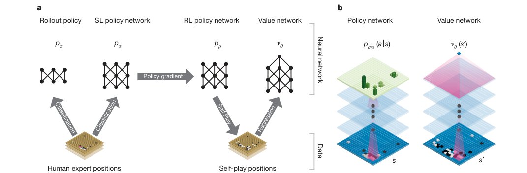
Figure 1 | Neural network training pipeline and architecture. a, A fast rollout policy $p_\pi$ and supervised learning (SL) policy network $p_\sigma$ are trained to predict human expert moves in a data set of positions. A reinforcement learning (RL) policy network $p_\rho$ is initialized to the SL policy network, and is then improved by policy gradient learning to maximize the outcome (that is, winning more games) against previous versions of the policy network. A new data set is generated by playing games of self-play with the RL policy network. Finally, a value network $v_\theta$ is trained by regression to predict the expected outcome (that is, whether the current player wins) in positions from the self-play data set. b, Schematic representation of the neural network architecture used in AlphaGo. The policy network takes a representation of the board position $s$ as its input, passes it through many convolutional layers with parameters $\sigma$ (SL policy network) or $\rho$ (RL policy network), and outputs a probability distribution $p_\sigma(a|s)$ or $p_\rho(a|s)$ over legal moves $a$, represented by a probability map over the board. The value network similarly uses many convolutional layers with parameters $\theta$, but outputs a scalar value $v_\theta(s')$ that predicts the expected outcome in position $s'$.

图 1 | 神经网络训练流水线与结构。a，快速走子策略 $p_\pi$ 与监督学习（SL）策略网络 $p_\sigma$ 在一个局面数据集上训练，以预测人类高手着法。强化学习（RL）策略网络 $p_\rho$ 初始化为 SL 策略网络，再用策略梯度学习改进，以最大化对策略网络先前版本的对局结果（也就是赢下更多对局）。随后用 RL 策略网络进行自我对弈，生成新的数据集。最后，价值网络 $v_\theta$ 通过回归训练，预测自我对弈数据集中各局面的期望结果（也就是当前棋手是否获胜）。b，AlphaGo 所用神经网络结构的示意图。策略网络以棋盘局面 $s$ 的表示作为输入，经过许多带参数 $\sigma$（SL 策略网络）或 $\rho$（RL 策略网络）的卷积层，输出合法着法 $a$ 上的概率分布 $p_\sigma(a|s)$ 或 $p_\rho(a|s)$，表示为棋盘上的概率图。价值网络同样使用许多带参数 $\theta$ 的卷积层，但输出标量价值 $v_\theta(s')$，预测局面 $s'$ 的期望结果。

Figure 2 | Strength and accuracy of policy and value networks. a, Plot showing the playing strength of policy networks as a function of their training accuracy. Policy networks with 128, 192, 256 and 384 convolutional filters per layer were evaluated periodically during training; the plot shows the winning rate of AlphaGo using that policy network against the match version of AlphaGo. b, Comparison of evaluation accuracy between the value network and rollouts with different policies. Positions and outcomes were sampled from human expert games. Each position was evaluated by a single forward pass of the value network $v_\theta$, or by the mean outcome of 100 rollouts, played out using either uniform random rollouts, the fast rollout policy $p_\pi$, the SL policy network $p_\sigma$ or the RL policy network $p_\rho$. The mean squared error between the predicted value and the actual game outcome is plotted against the stage of the game (how many moves had been played in the given position).

图 2 | 策略网络与价值网络的棋力与准确率。a，策略网络棋力随训练准确率变化的图。每层分别有 128、192、256 与 384 个卷积滤波器的策略网络在训练过程中被定期评估；图中给出使用该策略网络的 AlphaGo 对阵比赛版本 AlphaGo 的胜率。b，价值网络与不同策略走子之间的评估准确率比较。局面与结果采样自人类高手对局。每个局面由价值网络 $v_\theta$ 的单次前向传播评估，或由 100 次走子的平均结果评估，走子分别使用均匀随机走子、快速走子策略 $p_\pi$、SL 策略网络 $p_\sigma$ 或 RL 策略网络 $p_\rho$。预测价值与实际对局结果之间的均方误差，按对局阶段（该局面已经下了多少手）画出。

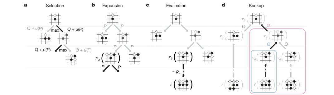
Figure 3 | Monte Carlo tree search in AlphaGo. a, Each simulation traverses the tree by selecting the edge with maximum action value $Q$, plus a bonus $u(P)$ that depends on a stored prior probability $P$ for that edge. b, The leaf node may be expanded; the new node is processed once by the policy network $p_\sigma$ and the output probabilities are stored as prior probabilities $P$ for each action. c, At the end of a simulation, the leaf node is evaluated in two ways: using the value network $v_\theta$; and by running a rollout to the end of the game with the fast rollout policy $p_\pi$, then computing the winner with function $r$. d, Action values $Q$ are updated to track the mean value of all evaluations $r(\cdot)$ and $v_\theta(\cdot)$ in the subtree below that action.

图 3 | AlphaGo 中的蒙特卡洛树搜索。a，每次模拟通过选择动作价值 $Q$ 加上奖励 $u(P)$ 最大的边来遍历树，该奖励依赖于这条边存储的先验概率 $P$。b，叶节点可以被扩展；新节点由策略网络 $p_\sigma$ 处理一次，输出概率作为每个动作的先验概率 $P$ 存储。c，一次模拟结束时，叶节点用两种方式评估：使用价值网络 $v_\theta$；以及用快速走子策略 $p_\pi$ 走到终局，再用函数 $r$ 计算胜者。d，动作价值 $Q$ 被更新，以跟踪该动作以下子树中所有评估 $r(\cdot)$ 与 $v_\theta(\cdot)$ 的平均值。

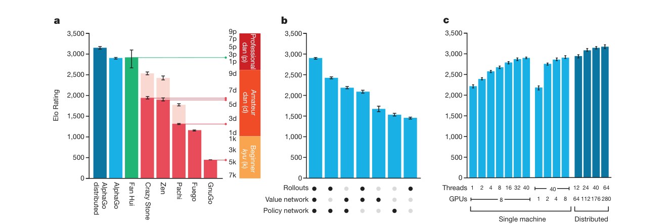
Figure 4 | Tournament evaluation of AlphaGo. a, Results of a tournament between different Go programs (see Extended Data Tables 6–11). Each program used approximately 5 s computation time per move. To provide a greater challenge to AlphaGo, some programs (pale upper bars) were given four handicap stones (that is, free moves at the start of every game) against all opponents. Programs were evaluated on an Elo scale$^{37}$: a 230 point gap corresponds to a 79% probability of winning, which roughly corresponds to one amateur dan rank advantage on KGS$^{38}$; an approximate correspondence to human ranks is also shown, horizontal lines show KGS ranks achieved online by that program. Games against the human European champion Fan Hui were also included; these games used longer time controls. 95% confidence intervals are shown. b, Performance of AlphaGo, on a single machine, for different combinations of components. The version solely using the policy network does not perform any search. c, Scalability study of MCTS in AlphaGo with search threads and GPUs, using asynchronous search (light blue) or distributed search (dark blue), for 2 s per move.

图 4 | AlphaGo 的循环赛评估。a，不同围棋程序之间循环赛的结果（见扩展数据表 6–11）。每个程序每步大约使用 5 秒计算时间。为给 AlphaGo 更大挑战，一些程序（浅色上段）对所有对手让四子（也就是每局开始时的免费着手）。程序按 Elo 分评估$^{37}$：230 分的差距对应 79% 的胜率，大约相当于 KGS 上一个业余段位的优势$^{38}$；图中也给出与人类段位的大致对应，水平线表示该程序在网上达到的 KGS 段位。对阵人类欧洲冠军樊麾的对局也包括在内；这些对局使用更长的时限。图中给出 95% 置信区间。b，单机 AlphaGo 在不同组件组合下的表现。只使用策略网络的版本不做任何搜索。c，AlphaGo 中 MCTS 随搜索线程与 GPU 变化的可扩展性研究，使用异步搜索（浅蓝色）或分布式搜索（深蓝色），每步 2 秒。

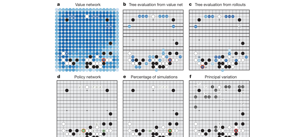
Figure 5 | How AlphaGo (black, to play) selected its move in an informal game against Fan Hui. For each of the following statistics, the location of the maximum value is indicated by an orange circle. a, Evaluation of all successors $s'$ of the root position $s$, using the value network $v_\theta(s')$; estimated winning percentages are shown for the top evaluations. b, Action values $Q(s, a)$ for each edge $(s, a)$ in the tree from root position $s$; averaged over value network evaluations only ($\lambda = 0$). c, Action values $Q(s, a)$, averaged over rollout evaluations only ($\lambda = 1$). d, Move probabilities directly from the SL policy network, $p_\sigma(a|s)$; reported as a percentage (if above 0.1%). e, Percentage frequency with which actions were selected from the root during simulations. f, The principal variation (path with maximum visit count) from AlphaGo’s search tree. The moves are presented in a numbered sequence. AlphaGo selected the move indicated by the red circle; Fan Hui responded with the move indicated by the white square; in his post-game commentary he preferred the move (labelled 1) predicted by AlphaGo.

图 5 | AlphaGo（执黑，该下）如何在与樊麾的一局非正式对局中选择着法。对下面每一项统计，最大值的位置用橙色圆圈标出。a，用价值网络 $v_\theta(s')$ 评估根局面 $s$ 的所有后继 $s'$；对评估最高的着法标出估计胜率。b，从根局面 $s$ 出发的树中每条边 $(s, a)$ 的动作价值 $Q(s, a)$；只对价值网络评估取平均（$\lambda = 0$）。c，动作价值 $Q(s, a)$，只对走子评估取平均（$\lambda = 1$）。d，直接来自 SL 策略网络的着法概率 $p_\sigma(a|s)$；以百分比给出（若高于 0.1%）。e，模拟中从根节点选出各动作的频率百分比。f，AlphaGo 搜索树中的主要变化（访问次数最大的路径）。着法按编号顺序给出。AlphaGo 选择了红圈标出的着法；樊麾应以白方块标出的着法；在赛后解说中，他更倾向于 AlphaGo 预测的那手（标为 1）。

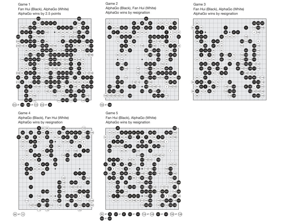
Figure 6 | Games from the match between AlphaGo and the European champion, Fan Hui. Moves are shown in a numbered sequence corresponding to the order in which they were played. Repeated moves on the same intersection are shown in pairs below the board. The first move number in each pair indicates when the repeat move was played, at an intersection identified by the second move number (see Supplementary Information).

图 6 | AlphaGo 与欧洲冠军樊麾对局中的棋谱。着法按实际落子顺序编号给出。同一交叉点上的重复落子在棋盘下方成对标出。每对中的第一个手数表示重复落子发生的时机，交叉点由第二个手数标明（见补充信息）。

Online Content Methods, along with any additional Extended Data display items and Source Data, are available in the online version of the paper; references unique to these sections appear only in the online paper.

在线内容 方法部分，以及任何额外的扩展数据展示项与源数据，可在论文的在线版本中获得；这些部分独有的参考文献只出现在在线论文中。

Received 11 November 2015; accepted 5 January 2016.

2015 年 11 月 11 日收到；2016 年 1 月 5 日接受。

Acknowledgements We thank Fan Hui for agreeing to play against AlphaGo; T. Manning for refereeing the match; R. Munos and T. Schaul for helpful discussions and advice; A. Cain and M. Cant for work on the visuals; P. Dayan, G. Wayne, D. Kumaran, D. Purves, H. van Hasselt, A. Barreto and G. Ostrovski for reviewing the paper; and the rest of the DeepMind team for their support, ideas and encouragement.

致谢 我们感谢樊麾同意与 AlphaGo 对弈；感谢 T. Manning 担任比赛裁判；感谢 R. Munos 与 T. Schaul 的有益讨论与建议；感谢 A. Cain 与 M. Cant 在可视化方面的工作；感谢 P. Dayan、G. Wayne、D. Kumaran、D. Purves、H. van Hasselt、A. Barreto 与 G. Ostrovski 审阅本文；并感谢 DeepMind 团队其余成员的支持、想法与鼓励。

Author Contributions A.H., G.v.d.D., J.S., I.A., M.La., A.G., T.G. and D.S. designed and implemented the search in AlphaGo. C.J.M., A.G., L.S., A.H., I.A., V.P., S.D., D.G., N.K., I.S., K.K. and D.S. designed and trained the neural networks in AlphaGo. J.S., J.N., A.H. and D.S. designed and implemented the evaluation framework for AlphaGo. D.S., M.Le., T.L., T.G., K.K. and D.H. managed and advised on the project. D.S., T.G., A.G. and D.H. wrote the paper.

Author Information Reprints and permissions information is available at www.nature.com/reprints. The authors declare no competing financial interests. Readers are welcome to comment on the online version of the paper. Correspondence and requests for materials should be addressed to D.S. (davidsilver@google.com) or D.H. (demishassabis@google.com).

METHODS

方法

Problem setting

问题设定

Many games of perfect information, such as chess, checkers, othello, backgammon and Go, may be defined as alternating Markov games$^{39}$. In these games, there is a state space $\mathcal{S}$ (where state includes an indication of the current player to play); an action space $\mathcal{A}(s)$ defining the legal actions in any given state $s \in \mathcal{S}$; a state transition function $f(s, a, \xi)$ defining the successor state after selecting action $a$ in state $s$ and random input $\xi$ (for example, dice); and finally a reward function $r_i(s)$ describing the reward received by player $i$ in state $s$. We restrict our attention to two-player zero-sum games, $r_1(s) = -r_2(s) = r(s)$, with deterministic state transitions, $f(s, a, \xi) = f(s, a)$, and zero rewards except at a terminal time step $T$. The outcome of the game $z_t = \pm r(s_T)$ is the terminal reward at the end of the game from the perspective of the current player at time step $t$. A policy $p(a|s)$ is a probability distribution over legal actions $a \in \mathcal{A}(s)$. A value function is the expected outcome if all actions for both players are selected according to policy $p$, that is, $v^p(s) = \mathbb{E}[z_t \mid s_t = s, a_{t\ldots T} \sim p]$. Zero-sum games have a unique optimal value function $v^*(s)$ that determines the outcome from state $s$ following perfect play by both players.

许多完全信息博弈，如国际象棋、跳棋、奥赛罗、西洋双陆棋与围棋，都可以定义为交替马尔可夫博弈$^{39}$。在这些博弈中，有状态空间 $\mathcal{S}$（状态中包含当前该谁下）；动作空间 $\mathcal{A}(s)$ 给出任一状态 $s \in \mathcal{S}$ 中的合法动作；状态转移函数 $f(s, a, \xi)$ 给出在状态 $s$ 选择动作 $a$ 并接受随机输入 $\xi$（例如骰子）后的后继状态；最后还有奖励函数 $r_i(s)$，描述棋手 $i$ 在状态 $s$ 收到的奖励。我们只关注双人零和博弈，$r_1(s) = -r_2(s) = r(s)$，状态转移是确定性的，$f(s, a, \xi) = f(s, a)$，除终止时间步 $T$ 外奖励为零。对局结果 $z_t = \pm r(s_T)$ 是终局时从时间步 $t$ 的当前棋手视角看到的终止奖励。策略 $p(a|s)$ 是合法动作 $a \in \mathcal{A}(s)$ 上的概率分布。价值函数是双方所有动作都按策略 $p$ 选择时的期望结果，即 $v^p(s) = \mathbb{E}[z_t \mid s_t = s, a_{t\ldots T} \sim p]$。零和博弈有唯一的最优价值函数 $v^*(s)$，它决定双方完美行棋时从状态 $s$ 出发的结果。

Prior work

先前工作

The optimal value function can be computed recursively by minimax (or equivalently negamax) search$^{40}$. Most games are too large for exhaustive minimax tree search; instead, the game is truncated by using an approximate value function $v(s) \approx v^*(s)$ in place of terminal rewards. Depth-first minimax search with alpha–beta pruning$^{40}$ has achieved superhuman performance in chess$^4$, checkers$^5$ and othello$^6$, but it has not been effective in Go$^7$.

最优价值函数可以通过极小极大（或等价的负极大）搜索递归计算$^{40}$。大多数博弈都太大，无法做穷尽的极小极大树搜索；于是用近似价值函数 $v(s) \approx v^*(s)$ 代替终止奖励来截断对局。带 alpha–beta 剪枝的深度优先极小极大搜索$^{40}$ 已在国际象棋$^4$、跳棋$^5$ 和奥赛罗$^6$ 中达到超人表现，但在围棋中并不有效$^7$。

Reinforcement learning can learn to approximate the optimal value function directly from games of self-play$^{39}$. The majority of prior work has focused on a linear combination $v_\theta(s) = \phi(s) \cdot \theta$ of features $\phi(s)$ with weights $\theta$. Weights were trained using temporal-difference learning$^{41}$ in chess$^{42,43}$, checkers$^{44,45}$ and Go$^{30}$; or using linear regression in othello$^6$ and Scrabble$^9$. Temporal-difference learning has also been used to train a neural network to approximate the optimal value function, achieving superhuman performance in backgammon$^{46}$; and achieving weak kyu-level performance in small-board Go$^{28,29,47}$ using convolutional networks.

强化学习可以直接从自我对弈中学习近似最优价值函数$^{39}$。先前工作大多关注特征 $\phi(s)$ 与权重 $\theta$ 的线性组合 $v_\theta(s) = \phi(s) \cdot \theta$。权重在国际象棋$^{42,43}$、跳棋$^{44,45}$ 与围棋$^{30}$ 中用时序差分学习$^{41}$ 训练；在奥赛罗$^6$ 与 Scrabble$^9$ 中则用线性回归。时序差分学习也被用来训练神经网络以近似最优价值函数，在西洋双陆棋中达到超人表现$^{46}$；在小组棋盘围棋中，用卷积网络达到了较弱的级位水平$^{28,29,47}$。

An alternative approach to minimax search is Monte Carlo tree search (MCTS)$^{11,12}$, which estimates the optimal value of interior nodes by a double approximation, $V_n(s) \approx v^{P_n}(s) \approx v^*(s)$. The first approximation, $V_n(s) \approx v^{P_n}(s)$, uses $n$ Monte Carlo simulations to estimate the value function of a simulation policy $P_n$. The second approximation, $v^{P_n}(s) \approx v^*(s)$, uses a simulation policy $P_n$ in place of minimax optimal actions. The simulation policy selects actions according to a search control function $\arg\max_a(Q_n(s, a) + u(s, a))$, such as UCT$^{12}$, that selects children with higher action values, $Q_n(s, a) = -V_n(f(s, a))$, plus a bonus $u(s, a)$ that encourages exploration; or in the absence of a search tree at state $s$, it samples actions from a fast rollout policy $p_\pi(a|s)$. As more simulations are executed and the search tree grows deeper, the simulation policy becomes informed by increasingly accurate statistics. In the limit, both approximations become exact and MCTS (for example, with UCT) converges$^{12}$ to the optimal value function $\lim_{n\to\infty} V_n(s) = \lim_{n\to\infty} v^{P_n}(s) = v^*(s)$. The strongest current Go programs are based on MCTS$^{13–15,36}$.

相对极小极大搜索的另一条路线是蒙特卡洛树搜索（MCTS）$^{11,12}$，它通过双重近似来估计内部节点的最优价值，$V_n(s) \approx v^{P_n}(s) \approx v^*(s)$。第一个近似 $V_n(s) \approx v^{P_n}(s)$ 用 $n$ 次蒙特卡洛模拟来估计模拟策略 $P_n$ 的价值函数。第二个近似 $v^{P_n}(s) \approx v^*(s)$ 用模拟策略 $P_n$ 代替极小极大最优动作。模拟策略按搜索控制函数 $\arg\max_a(Q_n(s, a) + u(s, a))$ 选择动作，例如 UCT$^{12}$，它选择动作价值 $Q_n(s, a) = -V_n(f(s, a))$ 更高的子节点，再加上鼓励探索的奖励 $u(s, a)$；若状态 $s$ 处还没有搜索树，则从快速走子策略 $p_\pi(a|s)$ 中采样动作。随着模拟增多、搜索树加深，模拟策略会得到越来越准确的统计量。在极限下，两个近似都变为精确，MCTS（例如配合 UCT）收敛$^{12}$ 到最优价值函数 $\lim_{n\to\infty} V_n(s) = \lim_{n\to\infty} v^{P_n}(s) = v^*(s)$。目前最强的围棋程序都以 MCTS 为基础$^{13–15,36}$。

MCTS has previously been combined with a policy that is used to narrow the beam of the search tree to high-probability moves$^{13}$; or to bias the bonus term towards high-probability moves$^{48}$. MCTS has also been combined with a value function that is used to initialize action values in newly expanded nodes$^{16}$, or to mix Monte Carlo evaluation with minimax evaluation$^{49}$. By contrast, AlphaGo’s use of value functions is based on truncated Monte Carlo search algorithms$^{8,9}$, which terminate rollouts before the end of the game and use a value function in place of the terminal reward. AlphaGo’s position evaluation mixes full rollouts with truncated rollouts, resembling in some respects the well-known temporal-difference learning algorithm TD($\lambda$). AlphaGo also differs from prior work by using slower but more powerful representations of the policy and value function; evaluating deep neural networks is several orders of magnitude slower than linear representations and must therefore occur asynchronously.

此前，MCTS 曾与策略结合，用来把搜索树的束宽收窄到高概率着法$^{13}$，或把奖励项偏向高概率着法$^{48}$。MCTS 也曾与价值函数结合，用来初始化新扩展节点中的动作价值$^{16}$，或把蒙特卡洛评估与极小极大评估混合$^{49}$。相比之下，AlphaGo 对价值函数的使用建立在截断蒙特卡洛搜索算法$^{8,9}$ 之上：在终局前结束走子，并用价值函数代替终止奖励。AlphaGo 的局面评估把完整走子与截断走子混合起来，在某些方面类似于著名的时序差分学习算法 TD($\lambda$)。AlphaGo 与先前工作的另一不同之处，是使用更慢但更强的策略与价值函数表示；评估深度神经网络比线性表示慢几个数量级，因此必须异步进行。

The performance of MCTS is to a large degree determined by the quality of the rollout policy. Prior work has focused on handcrafted patterns$^{50}$ or learning rollout policies by supervised learning$^{13}$, reinforcement learning$^{16}$, simulation balancing$^{51,52}$ or online adaptation$^{30,53}$; however, it is known that rollout-based position evaluation is frequently inaccurate$^{54}$. AlphaGo uses relatively simple rollouts, and instead addresses the challenging problem of position evaluation more directly using value networks.

MCTS 的表现在很大程度上取决于走子策略的质量。先前工作关注手工设计的模式$^{50}$，或通过监督学习$^{13}$、强化学习$^{16}$、模拟平衡$^{51,52}$ 或在线适应$^{30,53}$ 来学习走子策略；不过，人们已经知道基于走子的局面评估常常不准$^{54}$。AlphaGo 使用相对简单的走子，转而用价值网络更直接地处理局面评估这一难题。

Search algorithm

搜索算法

To efficiently integrate large neural networks into AlphaGo, we implemented an asynchronous policy and value MCTS algorithm (APV-MCTS). Each node $s$ in the search tree contains edges $(s, a)$ for all legal actions $a \in \mathcal{A}(s)$. Each edge stores a set of statistics, $\{P(s,a), N_v(s,a), N_r(s,a), W_v(s,a), W_r(s,a), Q(s,a)\}$, where $P(s, a)$ is the prior probability, $W_v(s, a)$ and $W_r(s, a)$ are Monte Carlo estimates of total action value, accumulated over $N_v(s, a)$ and $N_r(s, a)$ leaf evaluations and rollout rewards, respectively, and $Q(s, a)$ is the combined mean action value for that edge. Multiple simulations are executed in parallel on separate search threads. The APV-MCTS algorithm proceeds in the four stages outlined in Fig. 3.

为了把大型神经网络高效地纳入 AlphaGo，我们实现了一种异步的策略与价值 MCTS 算法（APV-MCTS）。搜索树中的每个节点 $s$ 包含所有合法动作 $a \in \mathcal{A}(s)$ 对应的边 $(s, a)$。每条边存储一组统计量 $\{P(s,a), N_v(s,a), N_r(s,a), W_v(s,a), W_r(s,a), Q(s,a)\}$，其中 $P(s, a)$ 是先验概率，$W_v(s, a)$ 与 $W_r(s, a)$ 分别是在 $N_v(s, a)$ 次叶评估与 $N_r(s, a)$ 次走子奖励上累积的总动作价值的蒙特卡洛估计，$Q(s, a)$ 则是该边的合成平均动作价值。多次模拟在不同搜索线程上并行执行。APV-MCTS 算法按图 3 所示的四个阶段进行。

Selection (Fig. 3a). The first in-tree phase of each simulation begins at the root of the search tree and finishes when the simulation reaches a leaf node at time step $L$. At each of these time steps, $t < L$, an action is selected according to the statistics in the search tree, $a_t = \arg\max_a\bigl(Q(s_t, a) + u(s_t, a)\bigr)$, using a variant of the PUCT algorithm$^{48}$, $u(s,a) = c_{\mathrm{puct}} P(s,a)\frac{\sqrt{\sum_b N_r(s,b)}}{1+N_r(s,a)}$, where $c_{\mathrm{puct}}$ is a constant determining the level of exploration; this search control strategy initially prefers actions with high prior probability and low visit count, but asymptotically prefers actions with high action value.

选择（图 3a）。每次模拟的第一段树内阶段从搜索树的根开始，到模拟在时间步 $L$ 到达叶节点时结束。在这些时间步 $t < L$ 的每一步，根据搜索树中的统计量选择动作 $a_t = \arg\max_a\bigl(Q(s_t, a) + u(s_t, a)\bigr)$，使用的是 PUCT 算法$^{48}$ 的一种变体，$u(s,a) = c_{\mathrm{puct}} P(s,a)\frac{\sqrt{\sum_b N_r(s,b)}}{1+N_r(s,a)}$，其中 $c_{\mathrm{puct}}$ 是决定探索程度的常数；这一搜索控制策略起初偏好先验概率高、访问次数低的动作，但在极限下偏好动作价值高的动作。

Evaluation (Fig. 3c). The leaf position $s_L$ is added to a queue for evaluation $v_\theta(s_L)$ by the value network, unless it has previously been evaluated. The second rollout phase of each simulation begins at leaf node $s_L$ and continues until the end of the game. At each of these time-steps, $t \geq L$, actions are selected by both players according to the rollout policy, $a_t \sim p_\pi(\cdot|s_t)$. When the game reaches a terminal state, the outcome $z_t = \pm r(s_T)$ is computed from the final score.

评估（图 3c）。除非叶局面 $s_L$ 此前已被评估，否则将它加入队列，等待价值网络计算 $v_\theta(s_L)$。每次模拟的第二段走子阶段从叶节点 $s_L$ 开始，一直持续到终局。在这些时间步 $t \geq L$，双方都按走子策略选择动作，$a_t \sim p_\pi(\cdot|s_t)$。对局到达终止状态时，由最终分数计算出发 $z_t = \pm r(s_T)$。

Backup (Fig. 3d). At each in-tree step $t \leq L$ of the simulation, the rollout statistics are updated as if it has lost $n_{vl}$ games, $N_r(s_t, a_t) \leftarrow N_r(s_t, a_t) + n_{vl}$; $W_r(s_t, a_t) \leftarrow W_r(s_t, a_t) - n_{vl}$; this virtual loss$^{55}$ discourages other threads from simultaneously exploring the identical variation. At the end of the simulation, the rollout statistics are updated in a backward pass through each step $t \leq L$, replacing the virtual losses by the outcome, $N_r(s_t, a_t) \leftarrow N_r(s_t, a_t) - n_{vl} + 1$; $W_r(s_t, a_t) \leftarrow W_r(s_t, a_t) + n_{vl} + z_t$. Asynchronously, a separate backward pass is initiated when the evaluation of the leaf position $s_L$ completes. The output of the value network $v_\theta(s_L)$ is used to update value statistics in a second backward pass through each step $t \leq L$, $N_v(s_t, a_t) \leftarrow N_v(s_t, a_t) + 1$, $W_v(s_t, a_t) \leftarrow W_v(s_t, a_t) + v_\theta(s_L)$. The overall evaluation of each state action is a weighted average of the Monte Carlo estimates, $Q(s,a) = (1-\lambda)\frac{W_v(s,a)}{N_v(s,a)} + \lambda\frac{W_r(s,a)}{N_r(s,a)}$, that mixes together the value network and rollout evaluations with weighting parameter $\lambda$. All updates are performed lock-free$^{56}$.

回传（图 3d）。在模拟的每个树内步骤 $t \leq L$，走子统计量先按输掉 $n_{vl}$ 局来更新，$N_r(s_t, a_t) \leftarrow N_r(s_t, a_t) + n_{vl}$；$W_r(s_t, a_t) \leftarrow W_r(s_t, a_t) - n_{vl}$；这种虚拟损失$^{55}$ 会阻止其他线程同时探索同一变化。模拟结束时，走子统计量沿每个步骤 $t \leq L$ 反向更新，用结果替换虚拟损失：$N_r(s_t, a_t) \leftarrow N_r(s_t, a_t) - n_{vl} + 1$；$W_r(s_t, a_t) \leftarrow W_r(s_t, a_t) + n_{vl} + z_t$。与此同时，当叶局面 $s_L$ 的评估完成时，会启动另一次反向传递。价值网络的输出 $v_\theta(s_L)$ 用于在第二次反向传递中更新每个步骤 $t \leq L$ 的价值统计量，$N_v(s_t, a_t) \leftarrow N_v(s_t, a_t) + 1$，$W_v(s_t, a_t) \leftarrow W_v(s_t, a_t) + v_\theta(s_L)$。每个状态–动作的总体评估是这些蒙特卡洛估计的加权平均，$Q(s,a) = (1-\lambda)\frac{W_v(s,a)}{N_v(s,a)} + \lambda\frac{W_r(s,a)}{N_r(s,a)}$，用权重参数 $\lambda$ 把价值网络评估与走子评估混合起来。所有更新都是无锁的$^{56}$。

Expansion (Fig. 3b). When the visit count exceeds a threshold, $N_r(s, a) > n_{\mathrm{thr}}$, the successor state $s' = f(s, a)$ is added to the search tree. The new node is initialized to $\{N(s', a) = N_r(s', a) = 0, W(s', a) = W_r(s', a) = 0, P(s', a) = p_\tau(a|s')\}$, using a tree policy $p_\tau(a|s')$ (similar to the rollout policy but with more features, see Extended Data Table 4) to provide placeholder prior probabilities for action selection. The position $s'$ is also inserted into a queue for asynchronous GPU evaluation by the policy network. Prior probabilities are computed by the SL policy network $p_\sigma^\beta(\cdot|s')$ with a softmax temperature set to $\beta$; these replace the placeholder prior probabilities, $P(s', a) \leftarrow p_\sigma^\beta(a|s')$, using an atomic update. The threshold $n_{\mathrm{thr}}$ is adjusted dynamically to ensure that the rate at which positions are added to the policy queue matches the rate at which the GPUs evaluate the policy network. Positions are evaluated by both the policy network and the value network using a mini-batch size of 1 to minimize end-to-end evaluation time.

扩展（图 3b）。当访问次数超过阈值 $N_r(s, a) > n_{\mathrm{thr}}$ 时，后继状态 $s' = f(s, a)$ 被加入搜索树。新节点初始化为 $\{N(s', a) = N_r(s', a) = 0, W(s', a) = W_r(s', a) = 0, P(s', a) = p_\tau(a|s')\}$，用树策略 $p_\tau(a|s')$（与走子策略类似但特征更多，见扩展数据表 4）为动作选择提供占位的先验概率。局面 $s'$ 也会插入队列，供策略网络在 GPU 上异步评估。先验概率由 softmax 温度设为 $\beta$ 的 SL 策略网络 $p_\sigma^\beta(\cdot|s')$ 计算；它们通过原子更新替换占位先验，$P(s', a) \leftarrow p_\sigma^\beta(a|s')$。阈值 $n_{\mathrm{thr}}$ 动态调节，以保证加入策略队列的局面速率与 GPU 评估策略网络的速率相匹配。策略网络与价值网络评估局面时都使用大小为 1 的小批次，以尽量缩短端到端评估时间。

We also implemented a distributed APV-MCTS algorithm. This architecture consists of a single master machine that executes the main search, many remote worker CPUs that execute asynchronous rollouts, and many remote worker GPUs that execute asynchronous policy and value network evaluations. The entire search tree is stored on the master, which only executes the in-tree phase of each simulation. The leaf positions are communicated to the worker CPUs, which execute the rollout phase of simulation, and to the worker GPUs, which compute network features and evaluate the policy and value networks. The prior probabilities of the policy network are returned to the master, where they replace placeholder prior probabilities at the newly expanded node. The rewards from rollouts and the value network outputs are each returned to the master, and backed up the originating search path.

我们还实现了分布式 APV-MCTS 算法。这一架构由一台执行主搜索的主机器、许多执行异步走子的远程工作 CPU，以及许多执行异步策略与价值网络评估的远程工作 GPU 组成。整棵搜索树存放在主机器上，主机器只执行每次模拟的树内阶段。叶局面被传送给执行走子阶段的工作 CPU，以及计算网络特征并评估策略与价值网络的工作 GPU。策略网络的先验概率返回给主机器，替换新扩展节点上的占位先验。走子奖励与价值网络输出也各自返回主机器，并沿原来的搜索路径回传。

At the end of search AlphaGo selects the action with maximum visit count; this is less sensitive to outliers than maximizing action value$^{15}$. The search tree is reused at subsequent time steps: the child node corresponding to the played action becomes the new root node; the subtree below this child is retained along with all its statistics, while the remainder of the tree is discarded. The match version of AlphaGo continues searching during the opponent’s move. It extends the search if the action maximizing visit count and the action maximizing action value disagree. Time controls were otherwise shaped to use most time in the middle-game$^{57}$. AlphaGo resigns when its overall evaluation drops below an estimated 10% probability of winning the game, that is, $\max_a Q(s, a) < -0.8$. AlphaGo does not employ the all-moves-as-first$^{10}$ or rapid action value estimation$^{58}$ heuristics used in the majority of Monte Carlo Go programs; when using policy networks as prior knowledge, these biased heuristics do not appear to give any additional benefit. In addition AlphaGo does not use progressive widening$^{13}$, dynamic komi$^{59}$ or an opening book$^{60}$. The parameters used by AlphaGo in the Fan Hui match are listed in Extended Data Table 5.

搜索结束时，AlphaGo 选择访问次数最大的动作；这比最大化动作价值对离群值更不敏感$^{15}$。搜索树在后续时间步被复用：与已下动作对应的子节点成为新的根节点；该子节点以下的子树及其全部统计量被保留，树的其余部分则丢弃。比赛版本的 AlphaGo 在对手思考时继续搜索。如果最大化访问次数的动作与最大化动作价值的动作不一致，它会延长搜索。除此之外，时限安排成把大部分时间用在中盘$^{57}$。当总体评估降到估计胜率低于 10% 时，也就是 $\max_a Q(s, a) < -0.8$ 时，AlphaGo 认输。AlphaGo 不采用大多数蒙特卡洛围棋程序使用的“所有着法视作先着”$^{10}$ 或快速动作价值估计$^{58}$ 启发式；在用策略网络作为先验知识时，这些有偏启发式似乎不会再带来额外好处。此外，AlphaGo 也不使用渐进加宽$^{13}$、动态贴目$^{59}$ 或开局库$^{60}$。樊麾比赛中 AlphaGo 使用的参数见扩展数据表 5。

Rollout policy

走子策略

The rollout policy $p_\pi(a|s)$ is a linear softmax policy based on fast, incrementally computed, local pattern-based features consisting of both ‘response’ patterns around the previous move that led to state $s$, and ‘non-response’ patterns around the candidate move $a$ in state $s$. Each non-response pattern is a binary feature matching a specific $3 \times 3$ pattern centred on $a$, defined by the colour (black, white, empty) and liberty count (1, 2, $\geq 3$) for each adjacent intersection. Each response pattern is a binary feature matching the colour and liberty count in a 12-point diamond-shaped pattern$^{21}$ centred around the previous move. Additionally, a small number of handcrafted local features encode common-sense Go rules (see Extended Data Table 4). Similar to the policy network, the weights $\pi$ of the rollout policy are trained from 8 million positions from human games on the Tygem server to maximize log likelihood by stochastic gradient descent. Rollouts execute at approximately 1,000 simulations per second per CPU thread on an empty board.

References

- Allis, L. V. Searching for Solutions in Games and Artificial Intelligence. PhD thesis, Univ. Limburg, Maastricht, The Netherlands (1994).
- van den Herik, H., Uiterwijk, J. W. & van Rijswijck, J. Games solved: now and in the future. Artif. Intell. 134, 277–311 (2002).
- Schaeffer, J. The games computers (and people) play. Advances in Computers 52, 189–266 (2000).
- Campbell, M., Hoane, A. & Hsu, F. Deep Blue. Artif. Intell. 134, 57–83 (2002).
- Schaeffer, J. et al. A world championship caliber checkers program. Artif. Intell. 53, 273–289 (1992).
- Buro, M. From simple features to sophisticated evaluation functions. In 1st International Conference on Computers and Games, 126–145 (1999).
- Müller, M. Computer Go. Artif. Intell. 134, 145–179 (2002).
- Tesauro, G. & Galperin, G. On-line policy improvement using Monte-Carlo search. In Advances in Neural Information Processing, 1068–1074 (1996).
- Sheppard, B. World-championship-caliber Scrabble. Artif. Intell. 134, 241–275 (2002).
- Bouzy, B. & Helmstetter, B. Monte-Carlo Go developments. In 10th International Conference on Advances in Computer Games, 159–174 (2003).
- Coulom, R. Efficient selectivity and backup operators in Monte-Carlo tree search. In 5th International Conference on Computers and Games, 72–83 (2006).
- Kocsis, L. & Szepesvári, C. Bandit based Monte-Carlo planning. In 15th European Conference on Machine Learning, 282–293 (2006).
- Coulom, R. Computing Elo ratings of move patterns in the game of Go. ICGA J. 30, 198–208 (2007).
- Baudiš, P. & Gailly, J.-L. Pachi: State of the art open source Go program. In Advances in Computer Games, 24–38 (Springer, 2012).
- Enzenberger, M., Müller, M., Arneson, B. & Segal, R. Fuego – an open-source framework for board games and Go engine based on Monte-Carlo tree search. IEEE Trans. Comput. Intell. AI in Games 2, 259–270 (2010).
- Gelly, S. & Silver, D. Combining online and offline learning in UCT. In 17th International Conference on Machine Learning, 273–280 (2007).
- Krizhevsky, A., Sutskever, I. & Hinton, G. ImageNet classification with deep convolutional neural networks. In Advances in Neural Information Processing Systems, 1097–1105 (2012).
- Lawrence, S., Giles, C. L., Tsoi, A. C. & Back, A. D. Face recognition: a convolutional neural-network approach. IEEE Trans. Neural Netw. 8, 98–113 (1997).
- Mnih, V. et al. Human-level control through deep reinforcement learning. Nature 518, 529–533 (2015).
- LeCun, Y., Bengio, Y. & Hinton, G. Deep learning. Nature 521, 436–444 (2015).
- Stern, D., Herbrich, R. & Graepel, T. Bayesian pattern ranking for move prediction in the game of Go. In International Conference of Machine Learning, 873–880 (2006).
- Sutskever, I. & Nair, V. Mimicking Go experts with convolutional neural networks. In International Conference on Artificial Neural Networks, 101–110 (2008).
- Maddison, C. J., Huang, A., Sutskever, I. & Silver, D. Move evaluation in Go using deep convolutional neural networks. 3rd International Conference on Learning Representations (2015).
- Clark, C. & Storkey, A. J. Training deep convolutional neural networks to play go. In 32nd International Conference on Machine Learning, 1766–1774 (2015).
- Williams, R. J. Simple statistical gradient-following algorithms for connectionist reinforcement learning. Mach. Learn. 8, 229–256 (1992).
- Sutton, R., McAllester, D., Singh, S. & Mansour, Y. Policy gradient methods for reinforcement learning with function approximation. In Advances in Neural Information Processing Systems, 1057–1063 (2000).
- Sutton, R. & Barto, A. Reinforcement Learning: an Introduction (MIT Press, 1998).
- Schraudolph, N. N., Dayan, P. & Sejnowski, T. J. Temporal difference learning of position evaluation in the game of Go. Adv. Neural Inf. Process. Syst. 6, 817–824 (1994).
- Enzenberger, M. Evaluation in Go by a neural network using soft segmentation. In 10th Advances in Computer Games Conference, 97–108 (2003).
- Silver, D., Sutton, R. & Müller, M. Temporal-difference search in computer Go. Mach. Learn. 87, 183–219 (2012).
- Levinovitz, A. The mystery of Go, the ancient game that computers still can’t win. Wired Magazine (2014).
- Mechner, D. All Systems Go. The Sciences 38, 32–37 (1998).
- Mandziuk, J. Computational intelligence in mind games. In Challenges for Computational Intelligence, 407–442 (2007).
- Berliner, H. A chronology of computer chess and its literature. Artif. Intell. 10, 201–214 (1978).
- Browne, C. et al. A survey of Monte-Carlo tree search methods. IEEE Trans. Comput. Intell. AI in Games 4, 1–43 (2012).
- Gelly, S. et al. The grand challenge of computer Go: Monte Carlo tree search and extensions. Commun. ACM 55, 106–113 (2012).
- Coulom, R. Whole-history rating: A Bayesian rating system for players of time-varying strength. In International Conference on Computers and Games, 113–124 (2008).
- KGS. Rating system math. http://www.gokgs.com/help/rmath.html.
- Littman, M. L. Markov games as a framework for multi-agent reinforcement learning. In 11th International Conference on Machine Learning, 157–163 (1994).
- Knuth, D. E. & Moore, R. W. An analysis of alpha-beta pruning. Artif. Intell. 6, 293–326 (1975).
- Sutton, R. Learning to predict by the method of temporal differences. Mach. Learn. 3, 9–44 (1988).
- Baxter, J., Tridgell, A. & Weaver, L. Learning to play chess using temporal differences. Mach. Learn. 40, 243–263 (2000).
- Veness, J., Silver, D., Blair, A. & Uther, W. Bootstrapping from game tree search. In Advances in Neural Information Processing Systems (2009).
- Samuel, A. L. Some studies in machine learning using the game of checkers II - recent progress. IBM J. Res. Develop. 11, 601–617 (1967).
- Schaeffer, J., Hlynka, M. & Jussila, V. Temporal difference learning applied to a high-performance game-playing program. In 17th International Joint Conference on Artificial Intelligence, 529–534 (2001).
- Tesauro, G. TD-gammon, a self-teaching backgammon program, achieves master-level play. Neural Comput. 6, 215–219 (1994).
- Dahl, F. Honte, a Go-playing program using neural nets. In Machines that learn to play games, 205–223 (Nova Science, 1999).
- Rosin, C. D. Multi-armed bandits with episode context. Ann. Math. Artif. Intell. 61, 203–230 (2011).
- Lanctot, M., Winands, M. H. M., Pepels, T. & Sturtevant, N. R. Monte Carlo tree search with heuristic evaluations using implicit minimax backups. In IEEE Conference on Computational Intelligence and Games, 1–8 (2014).
- Gelly, S., Wang, Y., Munos, R. & Teytaud, O. Modification of UCT with patterns in Monte-Carlo Go. Tech. Rep. 6062, INRIA (2006).
- Silver, D. & Tesauro, G. Monte-Carlo simulation balancing. In 26th International Conference on Machine Learning, 119 (2009).
- Huang, S.-C., Coulom, R. & Lin, S.-S. Monte-Carlo simulation balancing in practice. In 7th International Conference on Computers and Games, 81–92 (Springer-Verlag, 2011).
- Baier, H. & Drake, P. D. The power of forgetting: improving the last-good-reply policy in Monte Carlo Go. IEEE Trans. Comput. Intell. AI in Games 2, 303–309 (2010).
- Huang, S. & Müller, M. Investigating the limits of Monte-Carlo tree search methods in computer Go. In 8th International Conference on Computers and Games, 39–48 (2013).
- Segal, R. B. On the scalability of parallel UCT. Computers and Games 6515, 36–47 (2011).
- Enzenberger, M. & Müller, M. A lock-free multithreaded Monte-Carlo tree search algorithm. In 12th Advances in Computer Games Conference, 14–20 (2009).
- Huang, S.-C., Coulom, R. & Lin, S.-S. Time management for Monte-Carlo tree search applied to the game of Go. In International Conference on Technologies and Applications of Artificial Intelligence, 462–466 (2010).
- Gelly, S. & Silver, D. Monte-Carlo tree search and rapid action value estimation in computer Go. Artif. Intell. 175, 1856–1875 (2011).
- Baudiš, P. Balancing MCTS by dynamically adjusting the komi value. ICGA J. 34, 131 (2011).
- Baier, H. & Winands, M. H. Active opening book application for Monte-Carlo tree search in 19×19 Go. In Benelux Conference on Artificial Intelligence, 3–10 (2011).
- Dean, J. et al. Large scale distributed deep networks. In Advances in Neural Information Processing Systems, 1223–1231 (2012).
- Go ratings. http://www.goratings.org.