AlphaFold: Improved protein structure prediction using potentials from deep learning

AlphaFold：用深度学习势能改进蛋白质结构预测

Andrew W. Senior$^{1*}$, Richard Evans$^{1*}$, John Jumper$^{1*}$, James Kirkpatrick$^{1*}$, Laurent Sifre$^{1*}$, Tim Green$^1$, Chongli Qin$^1$, Augustin Žídek$^1$, Alexander W. R. Nelson$^1$, Alex Bridgland$^1$, Hugo Penedones$^1$, Stig Petersen$^1$, Karen Simonyan$^1$, Steve Crossan$^1$, Pushmeet Kohli$^1$, David T. Jones$^{2,3}$, David Silver$^1$, Koray Kavukcuoglu$^1$, Demis Hassabis$^1$

$^1$DeepMind, London, UK

$^2$The Francis Crick Institute, London, UK

$^3$University College London, London, UK

$^*$These authors contributed equally to this work.

Protein structure prediction aims to determine the three-dimensional shape of a protein from its amino acid sequence$^1$. This problem is of fundamental importance to biology as the structure of a protein largely determines its function$^2$ but can be hard to determine experimentally. In recent years, considerable progress has been made by leveraging genetic information: analysing the co-variation of homologous sequences can allow one to infer which amino acid residues are in contact, which in turn can aid structure prediction$^3$. In this work, we show that we can train a neural network to accurately predict the distances between pairs of residues in a protein which convey more about structure than contact predictions. With this information we construct a potential of mean force$^4$ that can accurately describe the shape of a protein. We find that the resulting potential can be optimised by a simple gradient descent algorithm, to realise structures without the need for complex sampling procedures. The resulting system, named AlphaFold, has been shown to achieve high accuracy, even for sequences with relatively few homologous sequences. In the most recent Critical Assessment of Protein Structure Prediction$^5$ (CASP13), a blind assessment of the state of the field of protein structure prediction, AlphaFold created high-accuracy structures (with TM-scores$^\dagger$ of 0.7 or higher) for 24 out of 43 free modelling domains whereas the next best method, using sampling and contact information, achieved such accuracy for only 14 out of 43 domains.

蛋白质结构预测的目标，是根据氨基酸序列确定蛋白质的三维形状$^1$。这个问题对生物学具有根本重要性：蛋白质的结构在很大程度上决定其功能$^2$，但实验测定往往很困难。近年来，借助遗传信息已取得可观进展：分析同源序列的共变异，可以推断哪些氨基酸残基彼此接触，进而帮助结构预测$^3$。本文表明，我们可以训练神经网络，准确预测蛋白质中残基对之间的距离；这类距离所携带的结构信息，比接触预测更丰富。据此，我们构造了一种平均力势（potential of mean force）$^4$，能够准确描述蛋白质的形状。我们发现，只需用简单的梯度下降算法优化这一势能，就可以得到三维结构，而不必依赖复杂的采样步骤。由此得到的系统被命名为 AlphaFold，即便在同源序列相对较少的情况下，也能达到很高的精度。在最近一次蛋白质结构预测关键评估$^5$（CASP13）——该领域的盲测评估——中，AlphaFold 在 43 个自由建模结构域里把 24 个做到了高精度（TM-score$^\dagger$ 不低于 0.7）；当时次优的方法依靠采样和接触信息，只达到 14/43。

AlphaFold represents a significant advance in protein structure prediction. We expect the increased accuracy of structure predictions for proteins to enable insights in understanding the function and malfunction of these proteins, especially in cases where no homologous proteins have been experimentally determined$^7$.

AlphaFold 代表了蛋白质结构预测的一次显著进展。我们预期，预测精度的提高将有助于理解这些蛋白质的功能与失能机制，尤其是在尚无同源蛋白质实验结构的情形下$^7$。

$^\dagger$Template Modelling score$^6$, between 0 and 1, measures the degree of match of the overall (backbone) shape of a proposed structure to a native structure.

$^\dagger$模板建模分数（Template Modelling score，TM-score）$^6$介于 0 与 1 之间，衡量所提出结构的整体（骨架）形状与天然结构的吻合程度。

Proteins are at the core of most biological processes. Since the function of a protein is dependent on its structure, understanding protein structure has been a grand challenge in biology for decades. While several experimental structure determination techniques have been developed and improved in accuracy, they remain difficult and time-consuming$^2$. As a result, decades of theoretical work has attempted to predict protein structure from amino acid sequences.

蛋白质处于大多数生物过程的核心。蛋白质的功能依赖于其结构，因此理解蛋白质结构几十年来一直是生物学的重大挑战。虽然多种实验测定结构的技术已经发展起来，精度也在提高，但这些方法仍然困难且耗时$^2$。因此，几十年来已有大量理论研究尝试从氨基酸序列预测蛋白质结构。

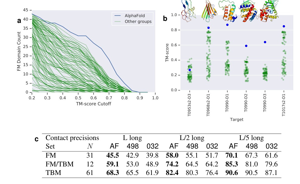
Fig. 1 | AlphaFold’s performance in the CASP13 assessment. (a) Number of free modelling (FM + FM/TBM) domains predicted to a given TM-score threshold for AlphaFold and the other 97 groups. (b) For the six new folds identified by the CASP13 assessors, AlphaFold’s TM-score compared with the other groups, with native structures. The structure of T1017s2-D1 is unavailable for publication. (c) Precisions for long-range contact prediction in CASP13 for the most probable $L$, $L/2$ or $L/5$ contacts, where $L$ is the length of the domain. The distance distributions used by AlphaFold (AF) in CASP13, thresholded to contact predictions, are compared with submissions by the two best-ranked contact prediction methods in CASP13: 498 (RaptorX-Contact$^8$) and 032 (TripletRes$^9$), on “all groups” targets, excluding T0999.

图 1｜AlphaFold 在 CASP13 评估中的表现。(a) 对 AlphaFold 以及其他 97 支队伍，达到给定 TM-score 阈值的自由建模（FM + FM/TBM）结构域数量。(b) 对 CASP13 评估人认定的 6 种新折叠，比较 AlphaFold 与其他队伍的 TM-score，并给出天然结构。T1017s2-D1 的结构不便公开发表。(c) CASP13 中长程接触预测的精度，分别取最可能的 $L$、$L/2$ 或 $L/5$ 个接触，其中 $L$ 是结构域长度。将 AlphaFold（AF）在 CASP13 中使用的距离分布按阈值转为接触预测后，与当时排名最高的两种接触预测方法的提交结果比较：498（RaptorX-Contact$^8$）和 032（TripletRes$^9$），对象为 “all groups” 靶标，不含 T0999。

Set	$N$	AF ($L$ long)	498 ($L$ long)	032 ($L$ long)	AF ($L/2$ long)	498 ($L/2$ long)	032 ($L/2$ long)	AF ($L/5$ long)	498 ($L/5$ long)	032 ($L/5$ long)
FM	31	45.5	42.9	39.8	58.0	55.1	51.7	70.1	67.3	61.6
FM/TBM	12	59.1	53.0	48.9	74.2	64.5	64.2	85.3	81.0	79.6
TBM	61	68.3	65.5	61.9	82.4	80.3	76.4	90.6	90.5	87.1

Table in Fig. 1c: Precisions for long-range contact prediction in CASP13.

Set	$N$	AF ($L$ long)	498 ($L$ long)	032 ($L$ long)	AF ($L/2$ long)	498 ($L/2$ long)	032 ($L/2$ long)	AF ($L/5$ long)	498 ($L/5$ long)	032 ($L/5$ long)
FM	31	45.5	42.9	39.8	58.0	55.1	51.7	70.1	67.3	61.6
FM/TBM	12	59.1	53.0	48.9	74.2	64.5	64.2	85.3	81.0	79.6
TBM	61	68.3	65.5	61.9	82.4	80.3	76.4	90.6	90.5	87.1

图 1c 中的表： CASP13 长程接触预测精度。

CASP$^5$ is a biennial blind protein structure prediction assessment run by the structure prediction community to benchmark progress in accuracy. In 2018, AlphaFold joined 97 groups from around the world in entering CASP13. Each group submitted up to 5 structure predictions for each of 84 protein sequences whose experimentally-determined structures were sequestered. Assessors divided the proteins into 104 domains for scoring and classified each as being amenable to template-based modelling (TBM, where a protein with a similar sequence has a known structure, and that homologous structure is modified in accordance with the sequence differences) or requiring free modelling (FM, when no homologous structure is available), with an intermediate (FM/TBM) category. Figure 1a shows that AlphaFold stands out in performance above the other entrants, predicting more FM domains to high accuracy than any other system, particularly in the 0.6–0.7 TM-score range.

CASP$^5$ 是由结构预测社区组织的两年一次盲测评估，用来衡量精度方面的进展。2018 年，AlphaFold 与来自世界各地的 97 支队伍一起参加了 CASP13。每支队伍要为 84 条蛋白质序列各提交至多 5 个结构预测，这些序列的实验结构在评估期间是封存的。评估人把蛋白质划分成 104 个结构域来打分，并把每个结构域归为两类：适合模板建模（TBM，即已有序列相似的蛋白质已知结构，再按序列差异去修改这个同源结构），或需要自由建模（FM，即没有可用的同源结构），另有中间类别（FM/TBM）。图 1a 显示，AlphaFold 的表现明显高出其他参赛者，把更多 FM 结构域做到了高精度，尤其是在 0.6–0.7 的 TM-score 区间。

The assessors ranked the 98 participating groups by the summed, capped $z$-scores of the structures, separated according to category. AlphaFold achieved a summed $z$-score of 52.8 in the FM category (best-of-5) vs 36.6 for the next closest group (322)$^\ddagger$. Combining FM and TBM/FM categories, AlphaFold scored 68.3 vs 48.2. AlphaFold is able to predict previously unknown folds to high accuracy as shown in Figure 1b. Despite using only free modelling techniques and not using templates, AlphaFold also scored well in the TBM category according to the assessors’ formula 0-capped $z$-score, ranking fourth by the top-1 model or first by the best-of-5 models. Much of the accuracy of AlphaFold is due to the accuracy of the distance predictions, which is evident from the high precision of the contact predictions of Table 1c.

评估人按各类别把结构的加总、截断 $z$ 分数加起来，对 98 支参赛队伍排序。AlphaFold 在 FM 类别（五选一最优）上的加总 $z$ 分数为 52.8，次近的队伍（322）为 36.6$^\ddagger$。把 FM 与 TBM/FM 两类合计，AlphaFold 为 68.3，对方为 48.2。如图 1b 所示，AlphaFold 能够以较高精度预测此前未知的折叠。尽管只用了自由建模技术、没有使用模板，AlphaFold 按评估人公式计算的 0 截断 $z$ 分数在 TBM 类别中也表现很好：按第一模型排第四，按五选一最优则排第一。AlphaFold 的精度很大程度上来自距离预测的精度，这从 Table 1c 中接触预测的高精确率就可以看出。

$^\ddagger$Results from http://predictioncenter.org/casp13/zscores_final.cgi?formula=assessors

$^\ddagger$结果来自 http://predictioncenter.org/casp13/zscores_final.cgi?formula=assessors

The most successful free modelling approaches so far$^{10–12}$ have relied on fragment assembly to determine the shape of the protein of interest. In these approaches a structure is created through a stochastic sampling process, such as simulated annealing$^{13}$, that minimises a statistical potential derived from summary statistics extracted from structures in the Protein Data Bank (PDB$^{14}$). In fragment assembly, a structure hypothesis is repeatedly modified, typically by changing the shape of a short section, retaining changes which lower the potential, ultimately leading to low potential structures. Simulated annealing requires many thousands of such moves and must be repeated many times to have good coverage of low-potential structures.

迄今最成功的自由建模方法$^{10–12}$，主要依靠片段组装来确定目标蛋白质的形状。这类方法通过随机采样过程——例如模拟退火$^{13}$——生成结构，并最小化由蛋白质数据银行（PDB$^{14}$）中结构的汇总统计量导出的统计势。在片段组装中，结构假设会被反复修改，通常是改变一小段的形状，保留能降低势能的改动，最终得到低势能结构。模拟退火需要成千上万次这样的移动，并且必须重复多次，才能较好地覆盖低势能结构。

In recent years, structure prediction accuracy has improved through the use of evolutionary covariation data$^{15}$ found in sets of related sequences. Sequences similar to the target sequence are found by searching large datasets of protein sequences derived from DNA sequencing and aligned to the target sequence to make a multiple sequence alignment (MSA). Correlated changes in two amino acid residue positions across the sequences of the MSA can be used to infer which residues might be in contact. Contacts are typically defined to occur when the $\beta$-carbon atoms of two residues are within 8 Å of one another. Several methods have been used to predict the probability that a pair of residues is in contact based on features computed from MSAs$^{16–19}$ including neural networks$^{20–23}$. Contact predictions are incorporated in structure prediction by modifying the statistical potential to guide the folding process to structures that satisfy more of the predicted contacts$^{12,24}$. Previous work$^{25,26}$ has made predictions of the distance between residues, particularly for distance geometry approaches$^{8,27–29}$. Neural network distance predictions without covariation features were used to make the EPAD potential$^{26}$ which was used for ranking structure hypotheses and the QUARK pipeline$^{12}$ used a template-based distance profile restraint for template-based modelling.

近年来，利用相关序列集合中的进化共变异数据$^{15}$，结构预测精度得到了提高。人们在由 DNA 测序得到的大规模蛋白质序列库中搜索与目标序列相似的序列，并与目标序列对齐，构成多序列比对（MSA）。MSA 各序列在两个氨基酸残基位置上的协同变化，可用来推断哪些残基可能相互接触。接触通常定义为两个残基的 $\beta$-碳原子相距在 8 Å 以内。已有多种方法根据从 MSA 算出的特征来预测残基对处于接触的概率$^{16–19}$，其中也包括神经网络$^{20–23}$。把接触预测纳入结构预测时，通常是修改统计势，引导折叠过程走向满足更多预测接触的结构$^{12,24}$。先前工作$^{25,26}$已经预测过残基之间的距离，尤其是在距离几何方法中$^{8,27–29}$。不使用共变异特征的神经网络距离预测被用来构造 EPAD 势$^{26}$，用于给结构假设排序；QUARK 流程$^{12}$则在模板建模中使用了基于模板的距离谱约束。

In this work we present a new, deep-learning, approach to protein structure prediction, whose stages are illustrated in Figure 2a. We show that it is possible to construct a learned, protein-specific potential by training a neural network (Fig. 2b) to make accurate predictions about the structure of the protein given its sequence, and to predict the structure itself accurately by minimising the potential by gradient descent (Fig. 2c). The neural network predictions include backbone torsion angles and pairwise distances between residues. Distance predictions provide more specific information about the structure than contact predictions and provide a richer training signal for the neural network. Predicting distances, rather than contacts as in most prior work, models detailed interactions rather than simple binary decisions. By jointly predicting many distances, the network can propagate distance information respecting covariation, local structure and residue identities to nearby residues. The predicted probability distributions can be combined to form a simple, principled protein-specific potential. We show that with gradient descent, it is simple to find a set of torsion angles that minimise this protein-specific potential using only limited sampling. We also show that whole chains can be optimised together, avoiding the need for segmenting long proteins into hypothesised domains which are modelled independently.

本文提出一种新的、基于深度学习的蛋白质结构预测方法，各阶段如图 2a 所示。我们表明：可以训练神经网络（图 2b），在给定序列的条件下对蛋白质结构作出准确预测，从而构造出学得的、针对该蛋白质的势能，再通过梯度下降最小化这一势能（图 2c），就能准确预测结构本身。神经网络的预测包括骨架扭角以及残基之间的成对距离。与接触预测相比，距离预测能给出更具体的结构信息，也给网络提供了更丰富的训练信号。预测距离而不是像多数先前工作那样预测接触，建模的是细致的相互作用，而不是简单的二元判定。通过联合预测许多距离，网络可以把兼顾共变异、局部结构和残基身份的距离信息传播到邻近残基。这些预测的概率分布可以组合起来，形成一个简单而有原则的蛋白质专属势。我们表明，用梯度下降只需有限采样，就可以找到一组使该蛋白质专属势取最小的扭角。我们还表明，整条链可以一起优化，不必再把长蛋白质切成假设的、再分别建模的结构域。

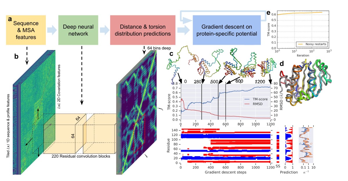
Fig. 2 | The folding process illustrated for CASP13 target T0986s2. (Length $L = 155$) (a) Steps of structure prediction. (b) The neural network predicts the entire $L \times L$ distogram based on MSA features, accumulating separate predictions for $64 \times 64$-residue regions. (c) One iteration of gradient descent (1 200 steps) is shown, with TM-score and RMSD plotted against step number with five snapshots of the structure. The secondary structure (from SST$^{30}$) is also shown (helix in blue, strand in red) along with the the native secondary structure (SS), the network’s secondary structure prediction probabilities and the uncertainty in torsion angle predictions (as $\kappa^{-1}$ of the von Mises distributions fitted to the predictions for $\phi$ and $\psi$). While each step of gradient descent greedily lowers the potential, large global conformation changes are effected, resulting in a well-packed chain. (d) shows the final first submission overlaid on the native structure (in grey). (e) shows the average (across the test set, $n = 377$) TM-score of the lowest-potential structure against the number of repeats of gradient descent (log scale).

图 2｜以 CASP13 靶标 T0986s2 说明折叠过程。（长度 $L = 155$）(a) 结构预测的各个步骤。(b) 神经网络根据 MSA 特征预测整张 $L \times L$ 距离图（distogram），并把对 $64 \times 64$ 残基区域的分别预测累积起来。(c) 展示一轮梯度下降（1 200 步），把 TM-score 和 RMSD 对步数作图，并给出五个结构快照。同时还给出二级结构（来自 SST$^{30}$；螺旋为蓝色，折叠股为红色），以及天然二级结构（SS）、网络的二级结构预测概率，和扭角预测的不确定性（对 $\phi$ 与 $\psi$ 的预测拟合 von Mises 分布后，取 $\kappa^{-1}$）。尽管梯度下降的每一步都在贪心地降低势能，仍能实现大幅度的整体构象变化，最终得到堆积良好的链。(d) 给出最终的第一提交结构，叠放在天然结构（灰色）上。(e) 给出测试集（$n = 377$）上最低势能结构的平均 TM-score 随梯度下降重复次数的变化（对数坐标）。

The central component of AlphaFold is a convolutional neural network which is trained on PDB structures to predict the distances $d_{ij}$ between the C$_\beta$ atoms of pairs, $ij$, of a protein’s residues. Based on a representation of the protein’s amino acid sequence, $\mathcal{S}$, and features derived from the sequence’s MSA, the network, similar in structure to those used for image recognition tasks$^{31}$, predicts a discrete probability distribution $P(d_{ij} \mid \mathcal{S}, \mathrm{MSA}(\mathcal{S}))$ for every $ij$ pair in a $64 \times 64$ residue region, as shown in Fig. 2b. The full set of distance distribution predictions is constructed by averaging predictions for overlapping regions and is termed a distogram (from distance histogram). Figure 3 shows an example distogram prediction for one CASP protein, T0955. The modes of the distribution (Fig. 3c) can be seen to closely match the true distances (Fig. 3b). Example distributions for all distances to one residue (29) are shown in Fig. 3c. Further analysis of how the network predicts the distances is shown in Methods Figure 14.

AlphaFold 的核心组件是一个卷积神经网络，在 PDB 结构上训练，用来预测蛋白质残基对 $ij$ 的 C$_\beta$ 原子之间的距离 $d_{ij}$。该网络的结构与图像识别任务中使用的网络类似$^{31}$，它根据蛋白质氨基酸序列 $\mathcal{S}$ 的表示以及由该序列 MSA 得到的特征，在 $64 \times 64$ 残基区域内为每一对 $ij$ 预测一个离散概率分布 $P(d_{ij} \mid \mathcal{S}, \mathrm{MSA}(\mathcal{S}))$，如图 2b 所示。对重叠区域的预测取平均，就得到完整的距离分布预测集合，称为距离图（distogram，由 distance histogram 而来）。图 3 给出了 CASP 蛋白质 T0955 的距离图预测示例。可以看到，分布的众数（图 3c）与真实距离（图 3b）非常接近。残基 29 到所有其他残基的距离分布示例见图 3c。关于网络如何预测这些距离的进一步分析，见方法部分的图 14。

In order to realise structures that conform to the distance predictions, we construct a smooth potential $V_{\mathrm{distance}}$ by fitting a spline to the negative log probabilities, and summing across all the residue pairs. We parameterise protein structures by the backbone torsion angles $(\boldsymbol{\phi}, \boldsymbol{\psi})$ of all residues and build a differentiable model of protein geometry $\mathbf{x} = G(\boldsymbol{\phi}, \boldsymbol{\psi})$ to compute the C$_\beta$ coordinates, $\mathbf{x}$, and thus the inter-residue distances, $d_{ij} = \lVert \mathbf{x}_i - \mathbf{x}_j \rVert$, for each structure, and express $V_{\mathrm{distance}}$ as a function of $\boldsymbol{\phi}$ and $\boldsymbol{\psi}$. For a protein with $L$ residues, this potential accumulates $L^2$ terms from marginal distribution predictions. To correct for the over-representation of the prior we subtract a reference distribution$^{32}$ from the distance potential in the log domain. The reference distribution models the distance distributions $P(d_{ij} \mid \mathrm{length})$ independent of the protein sequence and is computed by training a small version of the distance prediction neural network on the same structures, without sequence or MSA input features. A separate output head of the contact prediction network is trained to predict discrete probability distributions of backbone torsion angles $P(\phi_i, \psi_i \mid \mathcal{S}, \mathrm{MSA}(\mathcal{S}))$. After fitting a von Mises distribution, this is used to add a smooth torsion modelling term $V_{\mathrm{torsion}} = -\sum \log p_{\mathrm{vonMises}}(\phi_i, \psi_i \mid \mathcal{S}, \mathrm{MSA}(\mathcal{S}))$ to the potential. Finally, to prevent steric clashes, we add Rosetta’s $V_{\mathrm{score2\_smooth}}$$^{10}$ to the potential, as this incorporates a van der Waals term. We used multiplicative weights for each of the three terms in the potential, but no weighting noticeably outperformed equal weighting.

为了得到符合距离预测的结构，我们把负对数概率用样条拟合，再对所有残基对求和，从而构造出平滑势 $V_{\mathrm{distance}}$。我们用全部残基的骨架扭角 $(\boldsymbol{\phi}, \boldsymbol{\psi})$ 来参数化蛋白质结构，并建立可微的蛋白质几何模型 $\mathbf{x} = G(\boldsymbol{\phi}, \boldsymbol{\psi})$，用以计算 C$_\beta$ 坐标 $\mathbf{x}$，进而得到每个结构的残基间距离 $d_{ij} = \lVert \mathbf{x}_i - \mathbf{x}_j \rVert$，再把 $V_{\mathrm{distance}}$ 写成 $\boldsymbol{\phi}$ 与 $\boldsymbol{\psi}$ 的函数。对一条有 $L$ 个残基的蛋白质，该势会从边缘分布预测中累积 $L^2$ 项。为校正先验被过度表示的问题，我们在对数域中从距离势里减去一个参照分布$^{32}$。这个参照分布刻画的是不依赖于蛋白质序列的距离分布 $P(d_{ij} \mid \mathrm{length})$，其做法是在同一批结构上训练一个较小的距离预测网络，但不提供序列或 MSA 输入特征。接触预测网络另有一个输出头，用来预测骨架扭角的离散概率分布 $P(\phi_i, \psi_i \mid \mathcal{S}, \mathrm{MSA}(\mathcal{S}))$。拟合 von Mises 分布后，再用它给总势加上平滑的扭角建模项 $V_{\mathrm{torsion}} = -\sum \log p_{\mathrm{vonMises}}(\phi_i, \psi_i \mid \mathcal{S}, \mathrm{MSA}(\mathcal{S}))$。最后，为防止立体碰撞，我们把 Rosetta 的 $V_{\mathrm{score2\_smooth}}$$^{10}$ 加入势能，因为它包含范德瓦尔斯项。我们对势能中这三项使用了乘性权重，但没有任何加权明显优于等权。

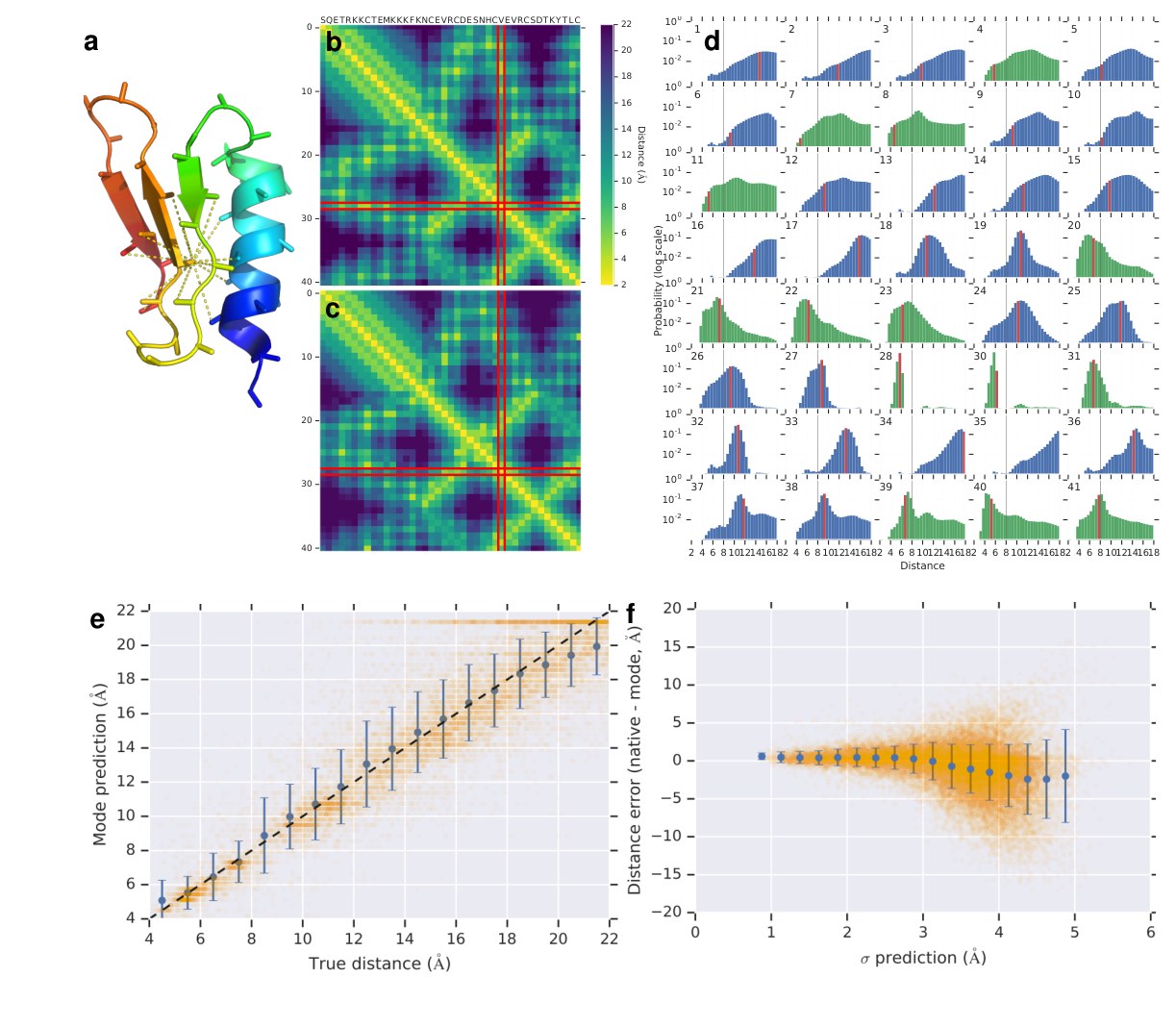
Fig. 3 | Predicted distance distributions compared with true distances. Above, for CASP target T0955 ($L = 41$): (a) Native structure showing distances under 8 Å from C$_\beta$ of residue 29. (b) Native inter-residue distances and (c) the mode of the distance predictions, highlighting residue 29. (d) The predicted probability distributions for distances of residue 29 to all other residues. The bin corresponding to the native distance is highlighted in red, 8 Å drawn in black. True contacts’ distributions are plotted in green, non-contacts in blue. Below, for CASP target T0990 ($L = 552$): (e) the mode of the predicted distance plotted against the true distance for all residue pairs with distances $\le 22$ Å, excluding distributions with standard deviation $> 3.5$ Å. The blue error bars show mean and standard deviation calculated for 1 Å bins. (f) The error of the mode distance prediction vs the standard deviation of the distance distributions, excluding pairs with native distances $>22$ Å). Mean and standard deviations are shown for 0.25 Å bins. The distogram is shown in Figure 7 in Methods.

图 3｜预测的距离分布与真实距离的比较。上半部分针对 CASP 靶标 T0955（$L = 41$）：(a) 天然结构，标出距残基 29 的 C$_\beta$ 不足 8 Å 的距离。(b) 天然残基间距离，以及 (c) 距离预测的众数，并突出残基 29。(d) 残基 29 到所有其他残基的预测距离概率分布。与天然距离对应的箱用红色标出，8 Å 用黑线标出。真接触的分布绘成绿色，非接触绘成蓝色。下半部分针对 CASP 靶标 T0990（$L = 552$）：(e) 对距离 $\le 22$ Å 的所有残基对，把预测距离的众数对真实距离作图，并排除标准差 $> 3.5$ Å 的分布。蓝色误差条给出按 1 Å 分箱计算的均值与标准差。(f) 众数距离预测的误差对距离分布标准差作图，排除天然距离 $>22$ Å 的残基对）。均值与标准差按 0.25 Å 分箱给出。距离图见方法部分的图 7。

Since all the terms in the combined potential $V_{\mathrm{total}}(\boldsymbol{\phi}, \boldsymbol{\psi})$ are differentiable functions of $(\boldsymbol{\phi}, \boldsymbol{\psi})$, it can be optimised with respect to these variables by gradient descent. Here we use L-BFGS$^{33}$. Structures are initialised by sampling torsion values from $P(\phi_i, \psi_i \mid \mathcal{S}, \mathrm{MSA}(\mathcal{S}))$. Figure 2c illustrates a single gradient descent trajectory minimising the potential, showing how this greedy optimisation process leads to increasing accuracy and large-scale conformation changes. Secondary structure is partly set by the initialisation, since some areas of secondary structure are predicted accurately, leading to low-variance torsion angle distributions. Overall accuracy (TM-score) improves quickly and after a few hundred steps of gradient descent has converged to a local optimum.

由于组合势 $V_{\mathrm{total}}(\boldsymbol{\phi}, \boldsymbol{\psi})$ 中的所有项都是 $(\boldsymbol{\phi}, \boldsymbol{\psi})$ 的可微函数，可以用梯度下降对这些变量做优化。这里我们使用 L-BFGS$^{33}$。结构的初始化，是从 $P(\phi_i, \psi_i \mid \mathcal{S}, \mathrm{MSA}(\mathcal{S}))$ 中采样扭角。图 2c 展示了一条最小化该势的梯度下降轨迹，说明这种贪心优化如何带来精度提升和大幅度构象变化。二级结构有一部分在初始化时就已经确定，因为某些二级结构区域预测较准，扭角分布的方差因此较低。整体精度（TM-score）提高很快，经过几百步梯度下降后就会收敛到一个局部最优。

We repeat the optimisation from sampled initialisations, leading to a pool of low potential structures from which further structure initialisations are sampled, with added backbone torsion noise (‘noisy restarts’), leading to more structures to be added to the pool. After only a few hundred cycles the optimisation converges and the lowest potential structure is chosen as the best candidate structure. Figure 2e shows the progress in the accuracy of the best-scoring structures over multiple restarts of the gradient descent process, showing that after a few iterations the optimisation has converged. Noisy restarts enable slightly higher TM-score structures to be found than when continuing to sample from the predicted torsion distributions (average of 0.641 vs 0.636 on our test set).

我们从采样得到的初始化反复做优化，形成一个低势能结构池，再从中采样新的结构初始化，并给骨架扭角加上噪声（“带噪声的重启”），从而把更多结构加入该池。只需几百轮，优化就会收敛，此时取势能最低的结构作为最佳候选。图 2e 给出多次重启梯度下降过程中最高分结构的精度变化，表明迭代几次后优化即已收敛。与继续从预测的扭角分布中采样相比，带噪声的重启能找到 TM-score 略高的结构（在我们的测试集上平均为 0.641 对 0.636）。

A key component of AlphaFold’s overall accuracy is that accurate distance predictions convey more information about structure than contact predictions. Figure 3e shows that the predictions of distance correlate well with the true distance. It can be seen from Figure 3f that the network is also modelling the uncertainty in its predictions. When the standard deviation of the predicted distribution is low, the predictions are more accurate. This is also evident in the predicted distributions of Figure 3d, where more confident predictions of the distance distribution (higher peak and lower standard deviation of the distribution) tend to be more accurate, with the true distance close to the peak. Broader, less-confidently-predicted distributions still assign probability to the correct value even when it is not close to the peak. The high accuracy of the distance predictions and consequently the contact predictions (Table 1c) comes from a combination of factors in the design of the neural network and its training, including predicting distances instead of contacts, data augmentation, feature representation, auxiliary losses, cropping and data curation. (See Methods section.)

AlphaFold 整体精度的一个关键，在于准确的距离预测比接触预测传达了更多结构信息。图 3e 表明，距离预测与真实距离相关性很好。从图 3f 还可以看出，网络也在对其预测的不确定性建模。当预测分布的标准差较低时，预测通常更准。这一点在图 3d 的预测分布里同样明显：更有把握的距离分布预测（峰值更高、分布的标准差更低）往往更准，真实距离靠近峰值。较宽、把握较小的分布即便峰值不靠近真值，仍会把概率分给正确取值。距离预测以及由此得到的接触预测（Table 1c）之所以精度高，来自神经网络设计及其训练中的多种因素，包括预测距离而非接触、数据增强、特征表示、辅助损失、裁剪以及数据整理。（见方法部分。）

Figure 4a shows that the distogram accuracy (measured by distogram lDDT$_{12}$, defined in Methods) correlates well with the TM-score of the final realised structures. Figure 4b shows the effect of changing the construction of the potential. Removing the distance potential entirely gives a TM-score of 0.266. Reducing the resolution of the distogram representation below 6 bins by averaging adjacent bins causes the TM-score to degrade. Removing the torsion potential, reference correction or $V_{\mathrm{score2\_smooth}}$ degrade the accuracy only slightly. A final ‘relaxation’ (side-chain packing interleaved with gradient descent) with Rosetta$^{10}$, using a combination of the Talaris2014 potential and a spline fit of our reference-corrected distance potential adds side-chain atom coordinates, and yields a small average improvement of 0.007 TM-score.

图 4a 表明，距离图精度（以方法部分定义的 distogram lDDT$_{12}$ 衡量）与最终实现结构的 TM-score 相关性很好。图 4b 给出了改变势能构造方式的影响。把距离势完全去掉，TM-score 只有 0.266。若把相邻箱平均，使距离图表示的分辨率降到 6 个箱以下，TM-score 会下降。去掉扭角势、参照校正或 $V_{\mathrm{score2\_smooth}}$，精度只略有下降。最后用 Rosetta$^{10}$ 做一次“弛豫”（把侧链堆积与梯度下降交错进行），势能为 Talaris2014 势与对我们做过参照校正的距离势的样条拟合的组合，这样可以补上侧链原子坐标，并使 TM-score 平均再提高 0.007。

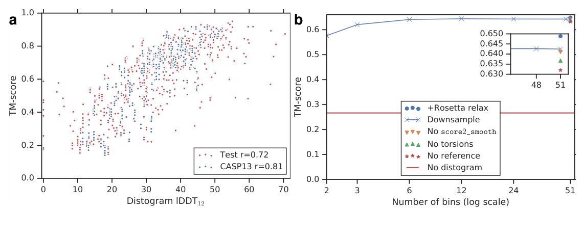
Fig. 4 | TM-scores vs the accuracy of the distogram, and the TM scores’ dependency on different components of the potential. (a) TM-score vs distogram lDDT$_{12}$ with Pearson’s correlation coefficients, for both CASP13 ($n = 108$) and test ($n = 377$) datasets. (b) Average TM-score over the test set ($n = 377$) vs number of histogram bins used when downsampling the distogram, compared with removing different components of the potential, or adding Rosetta relaxation.

图 4｜TM-score 与距离图精度的关系，以及 TM-score 对势能不同组成部分的依赖。(a) TM-score 对 distogram lDDT$_{12}$ 作图，并给出 Pearson 相关系数，数据集为 CASP13（$n = 108$）和测试集（$n = 377$）。(b) 测试集（$n = 377$）上的平均 TM-score 对降采样距离图时所用直方图箱数作图，并与去掉势能的不同组成部分、或加入 Rosetta 弛豫相比较。

We have shown that a carefully designed deep-learning system can provide accurate predictions of inter-residue distances and be used to construct a protein-specific potential which represents protein structure. Furthermore we have shown that this potential can be simply optimised with gradient descent to achieve accurate structure predictions. While free modelling predictions only rarely approach the accuracy of experimental structures, the CASP13 assessment shows that the AlphaFold system achieves unprecedented free modelling accuracy and that this free modelling method can match the performance of template modelling approaches without using templates and is starting to reach the accuracy needed for biological understanding (see Methods). We hope that the methods we have described can be developed further and applied to benefit all areas of protein science with more accurate predictions for sequences of unknown structure.

我们表明，一套精心设计的深度学习系统能够准确预测残基间距离，并用来构造表示蛋白质结构的专属势。我们还表明，只需用梯度下降优化这一势能，就可以得到准确的结构预测。自由建模预测虽然还很少能接近实验结构的精度，但 CASP13 评估表明，AlphaFold 系统达到了前所未有的自由建模精度；这种不使用模板的自由建模方法，已能与模板建模方法的表现相当，并开始接近生物学理解所需的精度（见方法）。我们希望这里描述的方法能够继续发展，并以对未知结构序列更准确的预测，服务于蛋白质科学的各个领域。

References

参考文献

1. Dill, K., Ozkan, S. B., Shell, M. & Weikl, T. The protein folding problem. Annu. Rev. Biophys. 37, 289–316 (2008).

2. Dill, K. & MacCallum, J. The protein-folding problem, 50 years on. Science 338, 1042–1046 (2012).

3. Schaarschmidt, J., Monastyrskyy, B., Kryshtafovych, A. & Bonvin, A. M. Assessment of contact predictions in CASP12: Co-evolution and deep learning coming of age. Proteins 86, 51–66 (2018).

4. Kirkwood, J. Statistical mechanics of fluid mixtures. J. Chem. Phys. 3, 300–313 (1935).

5. Moult, J., Fidelis, K., Kryshtafovych, A., Schwede, T. & Tramontano, A. Critical assessment of methods of protein structure prediction (CASP)—Round XII. Proteins: Structure, Function, and Bioinformatics 86, 7–15 (2018).

6. Zhang, Y. & Skolnick, J. Scoring function for automated assessment of protein structure template quality. Proteins 57, 702–710 (2004).

7. Zhang, Y. Protein structure prediction: when is it useful? Current opinion in structural biology 19, 145–155 (2009).

8. Xu, J. Protein structure modeling by predicted distance instead of contacts in CASP13 Abstracts Dec. 1, 2018 (2018), 146–7.

9. Zhang, C., Li, Y., Yu, D. & Zhang, Y. Contact map prediction by deep residual fully convolutional neural network with only evolutionary coupling features derived from deep multiple sequence alignment in CASP13 Abstracts Dec. 1, 2018 (2018), 181–2.

10. Das, R. & Baker, D. Macromolecular modeling with Rosetta. Annu. Rev. Biochem. 77, 363–382 (2008).

11. Jones, D. T. Predicting novel protein folds by using FRAGFOLD. Proteins 45, 127–132 (2001).

12. Zhang, C., Mortuza, S., He, B., Wang, Y. & Zhang, Y. Template-based and free modeling of I-TASSER and QUARK pipelines using predicted contact maps in CASP12. Proteins 86, 136–151 (2018).

13. Kirkpatrick, S., Gelatt, C. & Vecchi, M. Optimization by simulated annealing. Science 220, 671–680 (1983).

14. Gilliland, G. et al. The Protein Data Bank. Nucleic Acids Res. 28, 235–242 (2000).

15. Altschuh, D., Lesk, A., Bloomer, A. & Klug, A. Correlation of co-ordinated amino acid substitutions with function in viruses related to tobacco mosaic virus. J. Mol. Biol. 193, 693–707 (1987).

16. Ovchinnikov, S., Kamisetty, H. & Baker, D. Robust and accurate prediction of residue–residue interactions across protein interfaces using evolutionary information. Elife 3, e02030 (2014).

17. Seemayer, S., Gruber, M. & Söding, J. CCMpred—fast and precise prediction of protein residue–residue contacts from correlated mutations. Bioinformatics 30, 3128–3130 (2014).

18. Morcos, F. et al. Direct-coupling analysis of residue coevolution captures native contacts across many protein families. PNAS 108, E1293–E1301. ISSN: 0027-8424 (2011).

19. Jones, D. T., Buchan, D. W., Cozzetto, D. & Pontil, M. PSICOV: Precise structural contact prediction using sparse inverse covariance estimation on large multiple sequence alignments. Bioinformatics 28, 184–190 (2011).

20. Skwark, M., Raimondi, D., Michel, M. & Elofsson, A. Improved Contact Predictions Using the Recognition of Protein Like Contact Patterns. PLOS Computational Biology 10, 1–14 (2014).

21. Jones, D., Singh, T., Kosciolek, T. & Tetchner, S. MetaPSICOV: Combining coevolution methods for accurate prediction of contacts and long range hydrogen bonding in proteins. Bioinformatics 31, 999–1006 (2015).

22. Wang, S., Sun, S., Li, Z., Zhang, R. & Xu, J. Accurate De Novo Prediction of Protein Contact Map by Ultra-Deep Learning Model. PLoS Comput. Biol. 13, 999–1006 (2017).

23. Jones, D. T. & Kandathil, S. M. High precision in protein contact prediction using fully convolutional neural networks and minimal sequence features. Bioinformatics 1, 8 (2018).

24. Ovchinnikov, S. et al. Improved de novo structure prediction in CASP 11 by incorporating coevolution information into Rosetta. Proteins 84, 67–75 (2016).

25. Aszódi, A. & Taylor, W. R. Estimating polypeptide $\alpha$-carbon distances from multiple sequence alignments. J. Math. Chem. 17, 167–184 (1995).

26. Zhao, F. & Xu, J. A position-specific distance-dependent statistical potential for protein structure and functional study. Structure 20, 1118–1126 (2012).

27. Aszodi, A., Gradwell, M. & Taylor, W. Global fold determination from a small number of distance restraints. J. Mol. Biol. 251, 308–326 (1995).

28. Kandathil, S., Greener, J. & Jones, D. DMPfold: a new deep learning-based method for protein tertiary structure prediction and model refinement in CASP13 Abstracts Dec. 1, 2018 (2018), 84–5.

29. Xu, J. Distance-based Protein Folding Powered by Deep Learning. arXiv preprint arXiv:1811.03481 (2018).

30. Konagurthu, A. S., Lesk, A. M. & Allison, L. Minimum message length inference of secondary structure from protein coordinate data. Bioinformatics 28, i97–i105 (2012).

31. He, K., Zhang, X., Ren, S. & Sun, J. Deep Residual Learning for Image Recognition. arXiv preprint arXiv:1512.03385 abs/1512.03385 (2015).

32. Simons, K., Kooperberg, C., Huang, E. & Baker, D. Assembly of Protein Tertiary Structures from Fragments with Similar Local Sequences using Simulated Annealing and Bayesian Scoring Functions. J. Mol. Biol. 268, 209–225 (1997).

33. Liu, D. C. & Nocedal, J. On the limited memory BFGS method for large scale optimization. Math. Program. 45, 503–528 (1989).

1 Methods

1 方法

Figure 5 shows the steps involved in MSA construction, feature extraction, distance prediction, potential construction and structure realisation.

图 5 给出了 MSA 构建、特征抽取、距离预测、势能构造以及结构实现所涉及的各个步骤。

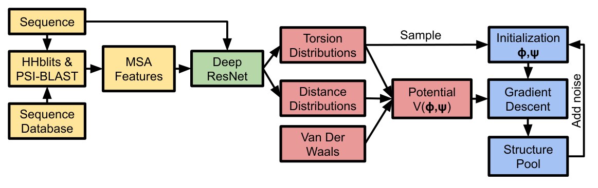
Fig. 5 | A schematic of the folding system. Feature extraction stages are shown in yellow, structure-prediction neural network in green, potential construction in red and structure realisation in blue.

图 5｜折叠系统示意图。特征抽取阶段为黄色，结构预测神经网络为绿色，势能构造为红色，结构实现为蓝色。

Data Our models are trained on structures extracted from the Protein Data Bank$^1$. We extract non-redundant domains by utilising the CATH$^2$ 35% sequence similarity cluster representatives. This gives 31 247 domains, which are split into train, and test sets (29 427 and 1 820 proteins respectively) keeping all domains from the same homologous superfamily (H-level in the CATH classification) in the same partition. The CATH superfamilies of FM domains from CASP11 and CASP12 were also excluded from the training set. From the test set, we take a single domain per homologous superfamily to create the 377 domain subset used for the results presented here. We note that accuracies for this set are higher than for the CASP13 test domains.

数据 我们的模型在从蛋白质数据银行（Protein Data Bank）$^1$ 抽取的结构上训练。我们利用 CATH$^2$ 的 35% 序列相似性聚类代表，抽取非冗余结构域，共得到 31 247 个结构域，再划分成训练集与测试集（分别为 29 427 和 1 820 个蛋白质），并把同一同源超家族（CATH 分类中的 H 级）的所有结构域放在同一分区。CASP11 和 CASP12 中 FM 结构域所属的 CATH 超家族也被排除在训练集之外。我们从测试集里每个同源超家族只取一个结构域，构成这里报告结果所用的 377 个结构域子集。需要说明的是，该集合上的精度高于 CASP13 测试结构域。

CASP13 submission results are drawn from the CASP13 results pages with additional results shown for the CASP13 dataset for “all groups” chains, scored on CASP13 PDB files, by CASP domain definitions. Contact prediction accuracies are recomputed from the group 032 and 498 submissions (as RR files), compared with the distogram predictions used by AlphaFold for CASP13 submissions. Contact prediction probabilities are obtained from the distograms by summing the probability mass in each distribution below 8 Å.

CASP13 提交结果取自 CASP13 结果页面；另外还给出了 CASP13 数据集上 “all groups” 链的补充结果，按 CASP 的结构域定义、在 CASP13 的 PDB 文件上计分。接触预测精度根据 032 组和 498 组的提交（RR 文件）重新计算，并与 AlphaFold 在 CASP13 提交中使用的距离图预测相比较。接触预测概率由距离图得到：把每个分布中 8 Å 以下的概率质量加起来。

For each training sequence, we search for and align similar protein sequences in the Uniclust30$^3$ dataset with HHblits$^4$ and use the returned MSA to generate profile features with the position-specific substitution probabilities for each residue as well as covariation features — the parameters of a regularised pseudolikelihood-trained Potts model similar to CCMPred$^5$. CCMPred uses the Frobenius norm of the parameters, but we feed both this norm (1 feature) as well as the raw parameters (484 features) into the network for each residue pair $ij$. In addition we provide the network with features explicitly representing gaps and deletions in the MSA. To make the network better able to make predictions for shallow MSAs, and as a form of data augmentation, we take a sample of half the sequences from the the HHblits MSA before computing the MSA-based features. Our training set contains 10 such samples for each domain. We extract additional profile features using PSI-BLAST$^6$.

对每条训练序列，我们用 HHblits$^4$ 在 Uniclust30$^3$ 数据集中搜索并对齐相似蛋白质序列，再用得到的 MSA 生成轮廓特征（每个残基的位置特异替换概率）以及共变异特征——即与 CCMPred$^5$ 类似、用正则化伪似然训练的 Potts 模型参数。CCMPred 使用这些参数的 Frobenius 范数，而我们则对每个残基对 $ij$，把该范数（1 维特征）和原始参数（484 维特征）都送入网络。此外，我们还向网络提供显式表示 MSA 中空位与缺失的特征。为了让网络在浅 MSA 上也能更好地预测，并作为一种数据增强，我们在计算基于 MSA 的特征之前，从 HHblits MSA 中抽取一半序列作为样本。每个结构域的训练集包含 10 个这样的样本。我们还用 PSI-BLAST$^6$ 抽取额外的轮廓特征。

The distance prediction neural network was trained with the following input features (with number of features).

距离预测神经网络使用下列输入特征进行训练（括号内为特征数）。

• Number of HHblits alignments (1D scalar)

• HHblits 比对条数（一维标量）

• Sequence-length features: 1-hot amino acid type (21D), Profiles: PSI-BLAST (21D), HHblits profile (22D), non-gapped profile (21D), HHblits bias, HMM profile (30D) Potts model bias (22D); Deletion probability (1D); residue index (integer index of residue number, consecutive except for multi-segment domains, encoded as 5 least-significant bits and a scalar);

• 序列长度特征：氨基酸类型的 one-hot（21 维），轮廓：PSI-BLAST（21 维）、HHblits 轮廓（22 维）、无空位轮廓（21 维）、HHblits 偏置、HMM 轮廓（30 维）、Potts 模型偏置（22 维）；缺失概率（1 维）；残基索引（残基编号的整数索引，除多段结构域外连续，编码为 5 个最低有效位再加一个标量）；

• Sequence-length-squared features: Potts model parameters (484D, fitted with 500 iterations of gradient descent using Nesterov momentum 0.99, without sequence reweighting); Frobenius norm (1D); Gap matrix (1D)

• 序列长度平方特征：Potts 模型参数（484 维，用 Nesterov 动量 0.99 做 500 次梯度下降拟合，不对序列重新加权）；Frobenius 范数（1 维）；空位矩阵（1 维）

Distogram prediction The inter-residue distances are predicted by a deep neural network. The architecture is a deep two-dimensional dilated convolutional residual network. Xu et al.$^7$ used a two-dimensional residual network preceded by one-dimensional embedding layers for contact prediction. Our network is two-dimensional throughout and uses 220 residual blocks$^8$ with dilated convolutions$^9$. Each residual block, illustrated in Figure 6 consists of a sequence of neural network layers$^{10}$, interleaving three batchnorm layers; two $1\times 1$ projection layers; a $3\times 3$ dilated convolution layer and ELU$^{11}$ nonlinearities. Successive layers cycle through dilations of 1, 2, 4, 8 pixels to allow propagation of information quickly across the cropped region. At the final layer, a position-specific bias was used, so the biases were indexed by residue-offset (capped at 32) and bin number.

距离图预测 残基间距离由一个深度神经网络预测。网络结构是深层的二维膨胀卷积残差网络。Xu 等人$^7$ 在接触预测中使用了前面加有一维嵌入层的二维残差网络。我们的网络全程都是二维的，并使用 220 个带膨胀卷积$^9$ 的残差块$^8$。每个残差块如图 6 所示，由一串神经网络层$^{10}$ 构成，交错安排三个批归一化层、两个 $1\times 1$ 投影层、一个 $3\times 3$ 膨胀卷积层，以及 ELU$^{11}$ 非线性。相邻层的膨胀率在 1、2、4、8 个像素间循环，以便信息能够迅速在裁剪区域中传播。最后一层使用位置特异偏置，因此偏置按残基偏移（上限为 32）和箱编号索引。

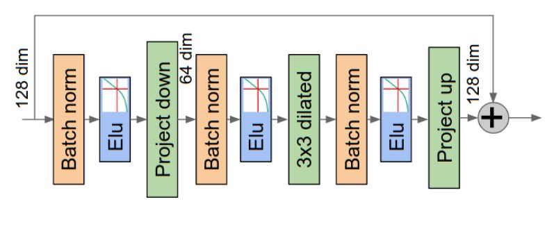
Fig. 6 | The layers used in one block of the deep residual convolutional network. The dilated convolution is applied on reduced-dimensional features. The output of the block is added to the representation from the previous layer. The residual network’s bypass connections allow gradients to pass back through the network undiminished, permitting the training of very deep networks.

图 6｜深度残差卷积网络中一个块所用的各层。膨胀卷积作用在降维后的特征上。该块的输出加到上一层的表示上。残差网络的旁路连接使梯度可以不受衰减地回传到网络中，从而能够训练非常深的网络。

The network is trained with stochastic gradient descent using a cross-entropy loss. The target is a quantisation of the distance between the residues’ C$_\beta$ atoms (C$_\alpha$ for glycine). We quantise the range 2–22 Å into 64 equal bins. The input to the network consists of a two-dimensional array of features where each $i, j$ feature is the concatenation of the 1-dimensional features for both $i$ and $j$ as well as the two-dimensional features for $i, j$.

网络用随机梯度下降训练，损失函数为交叉熵。训练目标是残基 C$_\beta$ 原子之间距离的量化（甘氨酸则用 C$_\alpha$）。我们把 2–22 Å 的范围等分成 64 个箱。网络的输入是一个二维特征阵列，其中每个 $i, j$ 特征是 $i$ 与 $j$ 各自的一维特征以及 $i, j$ 的二维特征的拼接。

Individual training runs were cross-validated with early stopping using 27 CASP11 FM domains as a validation set. Models were selected by cross-validation on 27 CASP12 FM domains.

各次训练用 27 个 CASP11 FM 结构域作为验证集，以早停做交叉验证。模型则按在 27 个 CASP12 FM 结构域上的交叉验证来选择。

Neural network hyperparameters

神经网络超参数

• $7 \times 4$ Blocks with 256 channels, cycling through dilations 1, 2, 4, 8

• $7 \times 4$ 个块，256 个通道，膨胀率在 1、2、4、8 间循环

• $48 \times 4$ Blocks with 128 channels, cycling through dilations 1, 2, 4, 8

• $48 \times 4$ 个块，128 个通道，膨胀率在 1、2、4、8 间循环

• Optimisation: Synchronized stochastic gradient descent

• 优化：同步随机梯度下降

• Batch size: batch of 4 crops on each of 8 GPU workers

• 批大小：8 个 GPU worker 上各 4 个裁块一批

• 0.85 Dropout keep probability

• Dropout 保留概率 0.85

• Nonlinearity: ELU

• 非线性：ELU

• Learning rate 0.06

• 学习率 0.06

• Auxilliary loss weights: Secondary structure: 0.005; Accessible surface area: 0.001. These auxilliary losses were cut by a factor 10 after 100 000 steps.

• 辅助损失权重：二级结构 0.005；可及表面积 0.001。这些辅助损失在 100 000 步之后减小到原来的 1/10。

• Learning rate decayed by 50% at 150 000, 200 000, 250 000 and 350 000 steps.

• 学习率在第 150 000、200 000、250 000 和 350 000 步时各衰减 50%。

• Training time: about 5 days for 600 000 steps

• 训练时间：约 5 天，共 600 000 步

To constrain memory usage and avoid overfitting, the network is always trained on $64 \times 64$ regions of the distance matrix, that is the pairwise distances between 64 consecutive residues and another group of 64 consecutive residues. For each training domain, the entire distance matrix is split into non-overlapping $64 \times 64$ crops. By training off-diagonal crops, the interaction between residues further apart than 64 residues can be modelled. Each crop consists of the distance matrix which represents the juxtaposition of two 64-residue fragments. Jones and Kandathil$^{12}$ have shown that contact prediction needs only a limited context window. We note that the distance predictions close to the diagonal $i = j$, encode predictions of the local structure of the protein, and for any cropped region the distances are governed by the local structure of the two fragments represented by the $i$ and $j$ ranges of the crop. Augmenting the inputs with the on-diagonal 2D input features that correspond to both the $i$ and $j$ ranges provides additional information to predict the structure of each fragment and thus distances between them. It can be seen that if the fragment structures can be well predicted (for instance if they are confidently predicted as helices or sheets) then prediction of a single contact between the fragments will strongly constrain the distances between all other pairs.

为了控制显存占用并避免过拟合，网络始终在距离矩阵的 $64 \times 64$ 区域上训练，也就是 64 个连续残基与另一组 64 个连续残基之间的成对距离。对每个训练结构域，整张距离矩阵被切成互不重叠的 $64 \times 64$ 裁块。通过对角线以外的裁块训练，可以建模相距超过 64 个残基的相互作用。每个裁块对应的距离矩阵，表示两段 64 残基片段的并置。Jones 和 Kandathil$^{12}$ 已经表明，接触预测只需要有限的上下文窗口。我们注意到，靠近对角线 $i = j$ 的距离预测编码的是蛋白质局部结构的预测；对任意裁块，其中的距离由该裁块 $i$、$j$ 范围所代表的两段片段的局部结构决定。把与 $i$、$j$ 范围相对应的对角二维输入特征补充进输入，可以为预测各片段结构、进而预测片段间距离提供额外信息。可以看出，如果片段结构能够被很好地预测（例如被有把握地预测为螺旋或折叠片），那么只要再预测片段之间的一个接触，就会强烈约束所有其他残基对的距离。

Randomising the offset of the crops each time a domain is used in training leads to a form of data augmentation where a single protein can generate many thousands of different training examples. This is further enhanced by adding noise to the atom coordinates, proportional to the ground truth resolution leading to variation in the target distances. Data augmentation (MSA subsampling and coordinate noise), together with dropout, prevents the network from overfitting to the training data.

每次把一个结构域用于训练时，随机化裁块的偏移，就形成一种数据增强：单个蛋白质可以产生成千上万个不同的训练样本。再按真实分辨率的比例给原子坐标加噪声，使目标距离产生变化，可以进一步增强这一点。数据增强（MSA 子采样和坐标噪声）再加上 dropout，可以防止网络在训练数据上过拟合。

To predict the distance distribution for all $L \times L$ residue pairs, many $64 \times 64$ crops are combined. To avoid edge effects, several such tilings are produced with different offsets and averaged together, with a heavier weighting for the predictions near the centre of the crop. To improve accuracy further, predictions from an ensemble of four separate models, trained independently with slightly different hyperparameters, are averaged together. Figure 7 shows an example of true distances (a) and the mode of the distogram prediction (b) for a three-domain CASP13 target.

为了预测全部 $L \times L$ 残基对的距离分布，需要把许多 $64 \times 64$ 裁块组合起来。为避免边缘效应，会用不同偏移做出若干次这样的铺贴再取平均，并对靠近裁块中心的预测给予更大权重。为进一步提高精度，还把四个独立训练、超参数略有不同的模型组成集成，对它们的预测再取平均。图 7 给出了一个三结构域 CASP13 靶标的示例：真实距离 (a) 与距离图预测的众数 (b)。

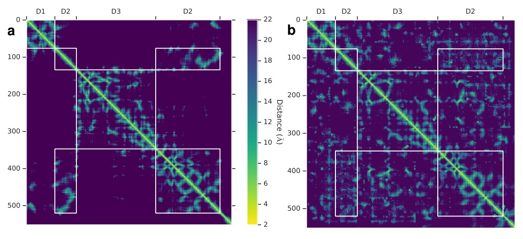
Fig. 7 | True distances (a) and modes of the predicted distogram (b) for CASP13 target T0990. CASP divides this chain into 3 domains as shown (D3 is inserted in D2) for which there are 39, 36 and 42 HHblits alignments respectively (from the CASP website).

图 7｜CASP13 靶标 T0990 的真实距离 (a) 与预测距离图的众数 (b)。如图所示，CASP 把这条链分成 3 个结构域（D3 插入在 D2 中），各自分别有 39、36 和 42 条 HHblits 比对（来自 CASP 网站）。

Since the network has a rich representation capable of incorporating both profile and covariation features of the MSA, we argue that the network can be used to predict secondary structure directly. By mean- and max-pooling the 2D activations of the penultimate layer of the network separately in both $i$ and $j$, we add an additional 1-dimensional output head to the network which predicts 8-class secondary structure labels as computed by DSSP$^{13}$ for each residue in $j$ and $i$. The resulting Q3 (distinguishing the three helix / sheet / coil classes) predictions’ accuracy is 84% which is comparable to the state-of-the-art$^{14}$. The relative accessible surface area (ASA) of each residue can also be predicted.

由于网络具有丰富的表示能力，能够同时纳入 MSA 的轮廓特征和共变异特征，我们认为它也可以直接用来预测二级结构。我们对网络倒数第二层的二维激活分别在 $i$ 和 $j$ 两个方向做均值池化和最大池化，从而为网络增加一个一维输出头，用来预测 $j$ 和 $i$ 中每个残基由 DSSP$^{13}$ 算出的 8 类二级结构标签。由此得到的 Q3（区分螺旋 / 折叠片 / 卷曲三类）预测精度为 84%，与当时最好水平相当$^{14}$。每个残基的相对可及表面积（ASA）也可以预测。

The 1-dimensional pooled activations are also used to predict the marginal Ramachandran distributions: $P(\phi_i, \psi_i \mid \mathcal{S}, \mathrm{MSA}(\mathcal{S}))$, independently for each residue, as a discrete probability distribution quantised to $10^\circ$ (1296 bins). In practice during CASP13 we used distograms from a network that was trained to predict distograms, secondary structure and ASA with torsions from a second, similar network trained to predict distograms, secondary structure, ASA and torsions, since the former had been more thoroughly validated.

一维池化后的激活还被用来预测边缘 Ramachandran 分布 $P(\phi_i, \psi_i \mid \mathcal{S}, \mathrm{MSA}(\mathcal{S}))$，对每个残基独立进行，作为按 $10^\circ$ 量化的离散概率分布（共 1296 个箱）。在 CASP13 期间，实际使用的距离图来自一个训练来预测距离图、二级结构和 ASA 的网络，扭角则来自第二个类似的、训练来预测距离图、二级结构、ASA 和扭角的网络，因为前者经过了更充分的验证。

Figure 8b shows that an important factor in the accuracy of the distograms (as has previously been found with contact prediction systems) is $N_{\mathrm{eff}}$, the effective number of sequences in the MSA$^{15}$. This is the number of sequences found in the MSA, discounting redundancy at the 62% sequence identity level, which we then divide by the number of residues in the target, and is an indication of the amount of covariation information in the MSA.

图 8b 表明，距离图精度的一个重要因素（这在接触预测系统中先前也已发现）是 $N_{\mathrm{eff}}$，即 MSA 中的有效序列数$^{15}$。它是 MSA 中在 62% 序列同一性水平上去除冗余后的序列数，再除以靶标的残基数，用来衡量 MSA 中共变异信息的多少。

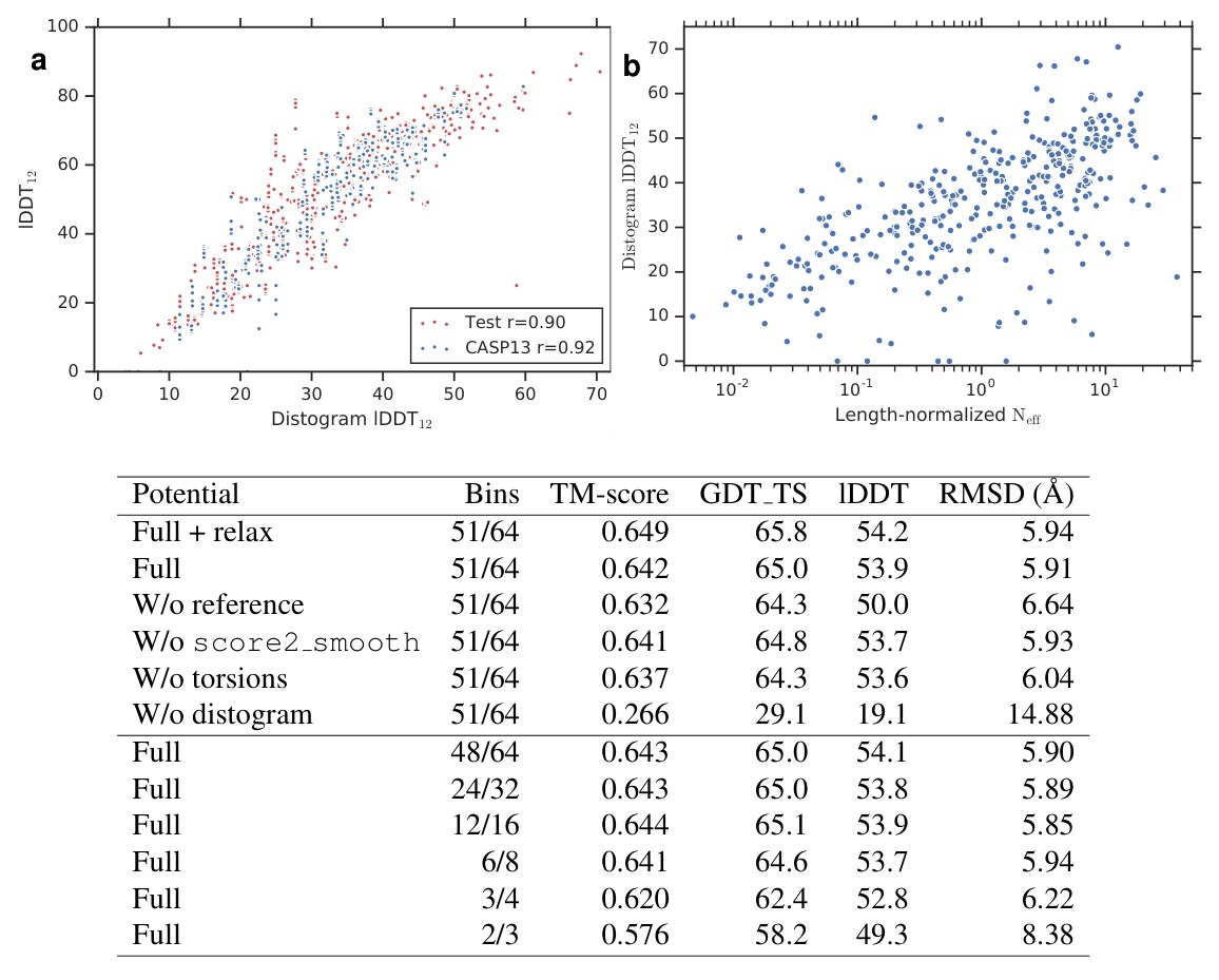
Fig. 8 | Analysis of structure accuracies. (a) lDDT vs distogram lDDT$_{12}$ (Defined below under ‘Accuracy’). The distogram accuracy predicts the realised structure’s lDDT (as well as TM-score as shown in Fig. 4a) well for both CASP13 ($n = 108$) and test ($n = 377$) datasets. Shown with Pearson’s correlation coefficients. (b) DLDDT$_{12}$ against effective number of sequences in the MSA ($N_{\mathrm{eff}}$) normalised by sequence length ($n = 377$). The number of effective sequences correlates with this measure of distogram accuracy ($r = 0.634$). (c) Structure accuracy measures, computed on the test set, for gradient descent optimisation of different forms of the potential. Above: Removing terms in the potential, also showing the effect of following optimisation with Rosetta relax. Bins shows the number of bins fitted by the spline before extrapolation and the number in the full distribution. In CASP13 splines were fitted to the first 51 of 64 bins. Below, reducing the resolution of the distogram distributions. The original 64-bin distogram predictions are repeatedly downsampled by a factor 2 by summing adjacent bins, in each case with constant extrapolation beyond 18 Å (the last $1/4$ of the bins). The final row’s two-level potential, designed to compare to contact predictions, is constructed by summing the probability mass below 8 Å and between 8–14 Å, with constant extrapolation beyond 14 Å. The TM-scores in this table are plotted in Figure 4 (b) Accuracy measures, computed on the test set ($n = 377$), for gradient descent optimisation with differently constructed potentials. The TM-scores in this table are plotted in Figure 4b.

图 8｜结构精度分析。(a) lDDT 对 distogram lDDT$_{12}$ 作图（定义见下文“精度”）。对 CASP13（$n = 108$）和测试集（$n = 377$），距离图精度都能很好地预测实现结构的 lDDT（以及图 4a 所示的 TM-score）。图中给出 Pearson 相关系数。(b) DLDDT$_{12}$ 对按序列长度归一化的 MSA 有效序列数（$N_{\mathrm{eff}}$）作图（$n = 377$）。有效序列数与这一距离图精度指标相关（$r = 0.634$）。(c) 在测试集上计算的结构精度指标，对应不同形式势能的梯度下降优化。上半部分：去掉势能中的各项，并给出优化后再做 Rosetta 弛豫的效果。Bins 表示外推之前由样条拟合的箱数，以及完整分布中的箱数。在 CASP13 中，样条拟合的是 64 个箱里的前 51 个。下半部分：降低距离图分布的分辨率。原来 64 箱的距离图预测反复按因子 2 降采样，即把相邻箱相加，每次都在 18 Å 以外做常数外推（最后 $1/4$ 的箱）。最后一行的两级势是为了与接触预测比较而设计的，做法是把 8 Å 以下以及 8–14 Å 之间的概率质量分别加总，并在 14 Å 以外做常数外推。该表中的 TM-score 绘于图 4。(b) 精度指标，在测试集（$n = 377$）上计算，对应以不同方式构造的势能的梯度下降优化。该表中的 TM-score 绘于图 4b。

Potential	Bins	TM-score	GDT TS	lDDT	RMSD (Å)
Full + relax	51/64	0.649	65.8	54.2	5.94
Full	51/64	0.642	65.0	53.9	5.91
W/o reference	51/64	0.632	64.3	50.0	6.64
W/o score2 smooth	51/64	0.641	64.8	53.7	5.93
W/o torsions	51/64	0.637	64.3	53.6	6.04
W/o distogram	51/64	0.266	29.1	19.1	14.88
Full	48/64	0.643	65.0	54.1	5.90
Full	24/32	0.643	65.0	53.8	5.89
Full	12/16	0.644	65.1	53.9	5.85
Full	6/8	0.641	64.6	53.7	5.94
Full	3/4	0.620	62.4	52.8	6.22
Full	2/3	0.576	58.2	49.3	8.38

Table in Fig. 8c: Accuracy measures, computed on the test set ($n = 377$), for gradient descent optimisation with differently constructed potentials. The TM-scores in this table are plotted in Figure 4b.

Potential	Bins	TM-score	GDT TS	lDDT	RMSD (Å)
Full + relax	51/64	0.649	65.8	54.2	5.94
Full	51/64	0.642	65.0	53.9	5.91
W/o reference	51/64	0.632	64.3	50.0	6.64
W/o score2 smooth	51/64	0.641	64.8	53.7	5.93
W/o torsions	51/64	0.637	64.3	53.6	6.04
W/o distogram	51/64	0.266	29.1	19.1	14.88
Full	48/64	0.643	65.0	54.1	5.90
Full	24/32	0.643	65.0	53.8	5.89
Full	12/16	0.644	65.1	53.9	5.85
Full	6/8	0.641	64.6	53.7	5.94
Full	3/4	0.620	62.4	52.8	6.22
Full	2/3	0.576	58.2	49.3	8.38

图 8c 中的表： 在测试集（$n = 377$）上，对以不同方式构造的势能做梯度下降优化得到的精度指标。该表中的 TM-score 绘于图 4b。

Distance potential The distogram probabilities are estimated for discrete distance bins, so to construct a differentiable potential the distribution is interpolated with a cubic spline. Because the final bin accumulates probability mass from all distances beyond 22 Å, and since greater distances are harder to predict accurately, the potential is only fit up to 18 Å (determined by cross-validation), with a constant extrapolation thereafter.

距离势 距离图概率是按离散距离箱估计的，因此要构造可微势，需用三次样条对分布做插值。由于最后一个箱会累积 22 Å 以外所有距离的概率质量，而且更远的距离更难准确预测，势能只拟合到 18 Å（由交叉验证确定），此后做常数外推。

To predict a reference distribution, a similar model is trained on the same dataset. The reference distribution is not conditioned on the sequence, but to account for the atoms between which we are predicting distances, we do provide a feature $\delta_{\alpha\beta}$ to indicate if the residue is glycine (C$_\alpha$ atom) or not (C$_\beta$) and the overall length of the protein.

为了预测参照分布，我们在同一数据集上训练一个类似的模型。参照分布不以序列为条件，但为了说明所预测距离两端是哪种原子，我们确实提供了特征 $\delta_{\alpha\beta}$，用来标明该残基是否为甘氨酸（C$_\alpha$ 原子，否则为 C$_\beta$），以及蛋白质的总长度。

A distance potential is created from the negative log likelihood of the distances, summed over all pairs of residues $i, j$.

距离势由各距离的负对数似然构成，并对所有残基对 $i, j$ 求和。

$$V_{\mathrm{distance}}(\mathbf{x}) = -\sum_{i,j,\, i \neq j} \log P(d_{ij} \mid \mathcal{S}, \mathrm{MSA}(\mathcal{S})) \tag{1}$$

With a reference state this becomes the log likelihood ratio of the distances under the full conditional model and under the background model:

引入参照态后，它变成距离在完整条件模型下与在背景模型下的对数似然比：

$$V_{\mathrm{distance}}(\mathbf{x}) = -\sum_{i,j,\, i \neq j} \log P(d_{ij} \mid \mathcal{S}, \mathrm{MSA}(\mathcal{S})) - \log P(d_{ij} \mid \mathrm{length}, \delta_{\alpha\beta}) \tag{2}$$

Torsions are modelled as a negative log likelihood under the predicted torsion distributions. Since we have marginal distribution predictions, each of which can be multimodal, it can be difficult to jointly optimise the torsions. To unify all the probability mass, at the cost of modelling fidelity of multimodal distributions, we fit a unimodal von Mises distribution to the marginal predictions. The potential is summed over all residues $i$.

扭角按预测扭角分布下的负对数似然来建模。由于我们只有边缘分布预测，而且每个都可能是多峰的，要联合优化这些扭角会比较困难。为了把全部概率质量统一起来，我们牺牲对多峰分布的刻画保真度，对边缘预测拟合单峰的 von Mises 分布。该势对所有残基 $i$ 求和。

$$V_{\mathrm{torsion}}(\boldsymbol{\phi}, \boldsymbol{\psi}) = -\sum_{i} \log p_{\mathrm{vonMises}}(\phi_i, \psi_i \mid \mathcal{S}, \mathrm{MSA}(\mathcal{S})) \tag{3}$$

Finally, to prevent steric clashes, a van der Waals term is introduced through the use of Rosetta’s $V_{\mathrm{score2\_smooth}}$.

最后，为防止立体碰撞，通过使用 Rosetta 的 $V_{\mathrm{score2\_smooth}}$ 引入范德瓦尔斯项。

Structure realisation by gradient descent To realise structures which minimise the constructed potential, we create a differentiable model of ideal protein backbone geometry, giving backbone atom coordinates as a function of the torsion angles $(\boldsymbol{\phi}, \boldsymbol{\psi})$: $\mathbf{x} = G(\boldsymbol{\phi}, \boldsymbol{\psi})$. The complete potential to be minimised is then$^*$:

用梯度下降实现结构 为了得到使所构造势能取最小的结构，我们建立了理想蛋白质骨架几何的可微模型，把骨架原子坐标写成扭角 $(\boldsymbol{\phi}, \boldsymbol{\psi})$ 的函数：$\mathbf{x} = G(\boldsymbol{\phi}, \boldsymbol{\psi})$。需要最小化的完整势因而为$^*$：

$$V_{\mathrm{total}}(\boldsymbol{\phi}, \boldsymbol{\psi}) = V_{\mathrm{distance}}(G(\boldsymbol{\phi}, \boldsymbol{\psi})) + V_{\mathrm{torsion}}(\boldsymbol{\phi}, \boldsymbol{\psi}) + V_{\mathrm{score2\_smooth}}(G(\boldsymbol{\phi}, \boldsymbol{\psi})). \tag{4}$$

$^*$While there is no guarantee that these potentials have equivalent scale, scaling parameters on the terms were introduced and chosen by cross-validation on CASP12 FM domains. In practice equal weighting for all terms was found to lead to the best results.

$^*$虽然不能保证这些势具有相当的尺度，我们仍为各项引入了缩放参数，并在 CASP12 FM 结构域上用交叉验证选定。实践中发现，对所有项等权可以得到最好结果。

Since every term in $V_{\mathrm{total}}$ is differentiable with respect to the torsion angles, given an initial set of torsions $\boldsymbol{\phi}, \boldsymbol{\psi}$ which can be sampled from the predicted torsion marginals, we can minimise $V_{\mathrm{total}}$ using a gradient descent algorithm, such as L-BFGS$^{16}$. The optimised structure is dependent on the initial conditions, so we repeat the optimisation multiple times with different initialisations. A pool of the 20 lowest-potential structures is maintained and once full, we initialise 90% of trajectories from those with $30^\circ$ noise added to the backbone torsions (the remaining 10% being sampled from the predicted torsion distributions). In CASP13 we made 5000 optimisation runs for each chain. Figure 2 shows the change in TM-score against the number of restarts. Since longer chains take longer to optimise, this work load was balanced across $(50+L)/2$ parallel workers. Figure 9 shows that this is achieved with a moderate computation budget, which can be parallelised over multiple machines.

由于 $V_{\mathrm{total}}$ 中的每一项都对扭角可微，给定一组可以从预测的扭角边缘分布中采样的初始扭角 $\boldsymbol{\phi}, \boldsymbol{\psi}$，就可以用梯度下降算法（例如 L-BFGS$^{16}$）来最小化 $V_{\mathrm{total}}$。优化得到的结构依赖于初始条件，因此我们用不同的初始化多次重复优化。我们维护一个由 20 个最低势能结构组成的池；池满之后，90% 的轨迹从这些结构初始化，并给骨架扭角加上 $30^\circ$ 噪声（其余 10% 则从预测的扭角分布中采样）。在 CASP13 中，我们对每条链做了 5000 次优化。图 2 给出了 TM-score 随重启次数的变化。由于更长的链优化更费时，这一工作负载在 $(50+L)/2$ 个并行 worker 之间做了均衡。图 9 表明，这是在中等计算预算下完成的，并且可以在多台机器上并行。

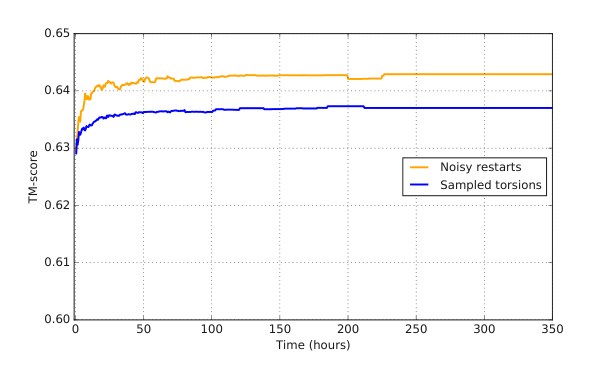
Fig. 9 | TM-score vs per-target computation time computed as an average over the test set ($n = 377$). Full optimisation with noisy restarts (orange) is compared with initialisation from sampled torsions (blue). Computation is measured as the product of the number of (CPU-based) machines and time elapsed and can be largely parallelised. Longer targets take longer to optimise.

图 9｜TM-score 对每个靶标的计算时间作图，时间为测试集（$n = 377$）上的平均值。带噪声重启的完整优化（橙色）与从采样扭角初始化（蓝色）相比较。计算量按（基于 CPU 的）机器数与所用时间的乘积来衡量，并且在很大程度上可以并行。更长的靶标优化耗时也更长。

Accuracy We compare the final structures to the experimentally determined structures to measure their accuracy using metrics such as TM-score, GDT TS$^{17}$ and RMSD. All of these accuracy measures require geometric alignment between the candidate structure and the experimental structure. An alternative accuracy measure which requires no alignment is the Local Distance Difference Test (lDDT$^{18}$) which measures the percentage of native pairwise distances $D_{ij}$ under 15 Å, with sequence offsets $\ge r$ residues, that are realised in a candidate structure (as $d_{ij}$) within a tolerance of the true value, averaging across tolerances of 0.5, 1, 2 and 4 Å (without stereochemical checks).

精度 我们把最终结构与实验测定结构相比较，用 TM-score、GDT TS$^{17}$ 和 RMSD 等指标来衡量精度。这些精度指标都需要对候选结构与实验结构做几何对齐。另一种不需要对齐的精度指标是局部距离差检验（Local Distance Difference Test，lDDT$^{18}$）：它衡量天然成对距离 $D_{ij}$ 中、距离在 15 Å 以内且序列偏移 $\ge r$ 个残基的那些，有百分之多少在候选结构里实现为 $d_{ij}$ 并且落在真值的容差范围内，再对 0.5、1、2 和 4 Å 这些容差取平均（不做立体化学检查）。

$$lDDT_r = \frac{100}{4L} \sum_{t \in \{0.5,1,2,4\}} \sum_{i=1}^{L} \frac{\sum_{j,\, |i-j|\ge r,\, D_{ij}<15} \mathbf{1}(|D_{ij}-d_{ij}|<t)}{\sum_{j,\, |i-j|\ge r,\, D_{ij}<15} 1}. \tag{5}$$

Since the distogram predicts pairwise distances, we can introduce distogram lDDT (DLDDT), a measure like lDDT computed directly from the distograms’ probabilities.

由于距离图预测的是成对距离，我们可以引入距离图 lDDT（DLDDT），这是一种类似 lDDT、但直接由距离图概率计算的指标。

$$DLDDT_r = \frac{100}{4L} \sum_{t \in \{0.5,1,2,4\}} \sum_{i=1}^{L} \frac{\sum_{j,\, |i-j|\ge r,\, D_{ij}<15} P(|D_{ij}-d_{ij}|<t \mid \mathcal{S}, \mathrm{MSA}(\mathcal{S}))}{\sum_{j,\, |i-j|\ge r,\, D_{ij}<15} 1} \tag{6}$$

Since distances between residues nearby in the sequence are often short, easier to predict and are not critical in determining the overall fold topology, we set $r = 12$, considering only those distances for residues with a sequence separation $\ge 12$. Since we predict C$_\beta$ distances, for this work we compute both lDDT and DLDDT using the C$_\beta$ distances.

由于序列上邻近的残基之间的距离往往较短、更容易预测，而且对整体折叠拓扑并不关键，我们取 $r = 12$，只考虑序列间隔 $\ge 12$ 的残基之间的距离。由于我们预测的是 C$_\beta$ 距离，本工作中的 lDDT 和 DLDDT 都用 C$_\beta$ 距离计算。

Full chains without domain segmentation Parameterising proteins of length $L$ by two torsion angles per residue, the dimension of space of structures grows as $2L$, so searching for structures of large proteins becomes much harder. Traditionally this problem is addressed by splitting longer protein chains into pieces, termed domains, which fold independently. However, the problem of domain segmentation from the sequence alone is itself difficult and error-prone. For this work, we avoided domain segmentation and folded entire chains. Typically multiple sequence alignments are based upon a given domain segmentation, but we used a sliding windows approach, computing a full-chain multiple sequence alignment to predict a baseline full-sequence distogram. We then compute MSAs for subsequences of the chain, trying windows of size 64, 128, 256 with offsets at multiples of 64. Each of these MSAs gives rise to an individual distogram corresponding to an on-diagonal square of the full-chain distogram. We average all these distograms together, weighted by the number of sequences in the MSA to produce an average full-chain distogram which is more accurate in regions where many alignments can be found.

不做结构域切分的完整链 用每个残基两个扭角来参数化长度为 $L$ 的蛋白质，结构空间的维数按 $2L$ 增长，因此搜索大型蛋白质的结构会困难得多。传统做法是把较长的蛋白质链切成称为结构域的片段，并假定它们独立折叠。然而，仅从序列做结构域切分本身就很困难，也容易出错。在本工作中，我们避免了结构域切分，直接折叠整条链。多序列比对通常依赖于给定的结构域切分，而我们采用滑动窗口方法：先计算整链的多序列比对，预测一个作为基线的全序列距离图；再对链的子序列计算 MSA，窗口大小取 64、128、256，偏移为 64 的倍数。每一个这样的 MSA 都会产生一张单独的距离图，对应于整链距离图对角线上的一个方块。我们按 MSA 中的序列数加权，把所有这些距离图平均起来，得到平均的整链距离图；在能够找到许多比对的区域，它更为准确。

CASP13 results In CASP13 the 5 AlphaFold submissions were from 3 different systems, all using potentials based on the neural network distance predictions. Before T0975, two systems based on simulated annealing and fragment assembly (and using 40 bin distance distributions) were used. From T0975 on, newly trained 64-bin distogram predictions were used and structures were generated by the gradient descent system described here (3 independent runs) as well as one of the fragment assembly systems (5 independent runs). 5 submissions were chosen from these 8 structures (the lowest potential structure generated by each independent run) with the first submission (‘top-1’) being the lowest-potential structure generated by gradient descent. The remaining four submissions were the four best other structures, with the fifth being a gradient descent structure if none had been chosen for position 2, 3 or 4. All submissions for T0999 were generated by gradient descent. Figure 10a shows the methods used for each submission, comparing with ‘back-fill’ structures generated by a single run of gradient descent for targets before T0975. Table 10b shows that the gradient descent method deployed later in CASP performed better than the fragment assembly method, in each category.

CASP13 结果 在 CASP13 中，AlphaFold 的 5 个提交来自 3 套不同系统，都使用基于神经网络距离预测的势能。在 T0975 之前，使用的是两套基于模拟退火和片段组装的系统（并用 40 箱的距离分布）。从 T0975 起，改用新训练的 64 箱距离图预测，结构则由本文所述的梯度下降系统生成（3 次独立运行），以及其中一套片段组装系统（5 次独立运行）。再从这 8 个结构（每次独立运行生成的最低势能结构）中选出 5 个提交，其中第一次提交（“top-1”）是梯度下降生成的最低势能结构。其余四次提交是另外四个最好的结构；如果第 2、3 或 4 位都没有选到梯度下降结构，则第五次提交用梯度下降结构。T0999 的全部提交都由梯度下降生成。图 10a 给出各次提交所用的方法，并与对 T0975 之前的靶标用单次梯度下降生成的“回填”结构相比较。表 10b 表明，后来在 CASP 中部署的梯度下降方法在每个类别上都优于片段组装方法。

Figure 10c compares the accuracy of the AlphaFold submissions for FM and FM/TBM domains with the next best group 322. For the CASP13 assessment full chains were relaxed with Rosetta relax with a potential of $V_{\mathrm{Talaris2014}} + 0.2 V_{\mathrm{distance}}$ (weighting determined by cross-validation) and submissions from all the systems were ranked based on this potential.

图 10c 把 AlphaFold 在 FM 和 FM/TBM 结构域上的提交精度，与次优的 322 组做比较。在 CASP13 评估中，完整链用 Rosetta relax 做了弛豫，所用势为 $V_{\mathrm{Talaris2014}} + 0.2 V_{\mathrm{distance}}$（权重由交叉验证确定），各系统的提交都按这一势能排序。

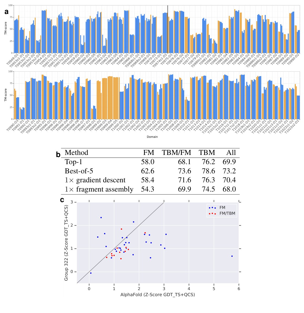
Fig. 10 | AlphaFold CASP13 results. (a) The TM-score for each of the 5 AlphaFold CASP13 submissions are shown. Simulated annealing with fragment assembly entries are shown in blue. Gradient-descent entries are shown in yellow. Gradient descent was only deployed for targets T0975 and later, so to the left of the black line we also show the results for a single, ‘back-fill’, run of gradient descent for each earlier target using the deployed system. T0999 (1589 residues) was manually segmented based on HHpred$^{19}$ homology matching. (b) Average TM-scores of the AlphaFold CASP13 submissions ($n = 104$ domains), comparing the first model submitted, the best-of-5 model (submission with highest GDT), a single run of full-chain gradient descent (a CASP13 run for T0975 and later, back-fill for earlier targets) and a single CASP13 run of fragment assembly with domain segmentation (using a gradient descent submission for T0999). (c) Assessors’ formula standardised ($z$) scores of GDT TS + QCS$^{20}$, best-of-5 for CASP FM ($n = 31$) and FM/TBM ($n = 12$) domains comparing AlphaFold with the closest competitor (group 322), coloured by domain category.

图 10｜AlphaFold 的 CASP13 结果。(a) 给出 AlphaFold 在 CASP13 中 5 次提交各自的 TM-score。模拟退火加片段组装的条目为蓝色，梯度下降条目为黄色。梯度下降只在 T0975 及之后的靶标上部署，因此在黑线左侧，我们还给出对更早靶标用已部署系统做一次“回填”梯度下降的结果。T0999（1589 个残基）是根据 HHpred$^{19}$ 同源匹配手工切分的。(b) AlphaFold CASP13 提交的平均 TM-score（$n = 104$ 个结构域），比较第一次提交的模型、五选一最优模型（GDT 最高的提交）、单次整链梯度下降（T0975 及之后为 CASP13 运行，更早靶标为回填），以及一次带结构域切分的 CASP13 片段组装运行（T0999 使用梯度下降提交）。(c) 按评估人公式计算的 GDT TS + QCS$^{20}$ 标准化（$z$）分数，取五选一最优，对象为 CASP 的 FM（$n = 31$）和 FM/TBM（$n = 12$）结构域，比较 AlphaFold 与最接近的竞争者（322 组），并按结构域类别着色。

Method	FM	TBM/FM	TBM	All
Top-1	58.0	68.1	76.2	69.9
Best-of-5	62.6	73.6	78.6	73.2
1× gradient descent	58.4	71.6	76.3	70.4
1× fragment assembly	54.3	69.9	74.5	68.0

Table in Fig. 10b: Average TM-scores of the AlphaFold CASP13 submissions ($n = 104$ domains).

Method	FM	TBM/FM	TBM	All
Top-1	58.0	68.1	76.2	69.9
Best-of-5	62.6	73.6	78.6	73.2
1× gradient descent	58.4	71.6	76.3	70.4
1× fragment assembly	54.3	69.9	74.5	68.0

图 10b 中的表： AlphaFold CASP13 提交的平均 TM-score（$n = 104$ 个结构域）。

Biological relevance There is a wide range of uses of predicted structures, all with different accuracy requirements, from generally understanding the fold shape to understanding detailed side-chain configurations in binding regions. Contact predictions alone can guide biological insight$^{21}$, for instance targeting mutations to destabilise the protein. The accuracy of the contact predictions shown in Table 1c indicates that the AlphaFold contact predictions exceed the state of the art. Here we present further results which indicate that AlphaFold’s accuracy improvements lead to more accurate interpretation of function; better interface prediction for protein-protein interaction; better binding pocket prediction and improved molecular replacement in crystallography.

生物学意义 预测结构的用途很广，对精度的要求也不相同，既包括大致理解折叠形状，也包括理解结合区域里细致的侧链构型。仅凭接触预测也可以指导生物学认识$^{21}$，例如针对会使蛋白质失稳的突变。Table 1c 中的接触预测精度表明，AlphaFold 的接触预测已经超过当时最好水平。这里我们再给出进一步结果，表明 AlphaFold 的精度提高可以带来更准确的功能解释、更好的蛋白质–蛋白质相互作用界面预测、更好的结合口袋预测，以及晶体学中更好的分子置换。

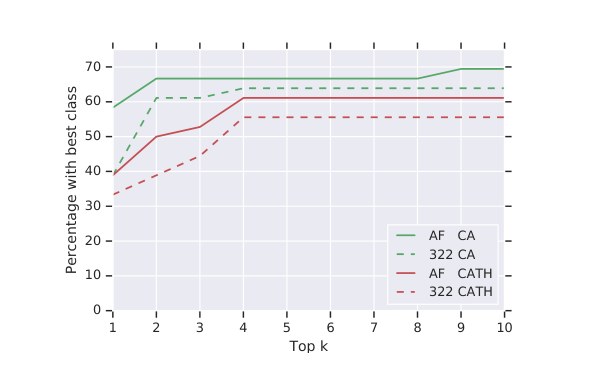
Fig. 11 | Correct fold identification by structural search in CATH. For each of the FM or TBM/FM domains, the top-1 submission and ground-truth are compared to all 30 744 CATH S40 non-redundant domains with TM-align$^{22}$. For the 36 domains where there is a good ground-truth match (score $> 0.5$), we show the percentage of decoys where a domain with the same CATH code (in red, CA in green. CAT results are close to CATH results) as the top ground-truth match is in the at-most top-$k$ matches with score $> 0.5$. Curves are shown for AlphaFold and the next-best group (322). AlphaFold predictions determine the matching fold more accurately. Determination of the matching CATH domain can give insight into the function of a new protein.

图 11｜在 CATH 中做结构检索以正确识别折叠。对每个 FM 或 TBM/FM 结构域，用 TM-align$^{22}$ 把 top-1 提交和真实结构与全部 30 744 个 CATH S40 非冗余结构域相比较。在 36 个具有良好真实匹配（分数 $> 0.5$）的结构域上，我们给出诱饵中的比例：与真实结构的最佳匹配具有相同 CATH 编码（红色；CA 为绿色。CAT 结果与 CATH 结果接近）的结构域，出现在分数 $> 0.5$ 的至多前 $k$ 个匹配中。曲线分别对应 AlphaFold 和次优组（322）。AlphaFold 的预测能更准确地确定相匹配的折叠。确定相匹配的 CATH 结构域，有助于认识新蛋白质的功能。

Often protein function can be inferred by finding homologous proteins of known function. Figure 11 shows that AlphaFold’s FM predictions give greater accuracy in structure-based search for homologous domains in the CATH database.

蛋白质功能常常可以通过寻找功能已知的同源蛋白质来推断。图 11 表明，AlphaFold 的 FM 预测在 CATH 数据库中基于结构搜寻同源结构域时精度更高。

Protein-protein interaction is an important domain for understanding protein function that has hitherto largely been limited to template-based models because of the need for high accuracy predictions, though there has been moderate success$^{23}$ in docking with predicted structures up to 6 Å RMSD. Figure 12 shows that AlphaFold’s predictions improve accuracy in the interface regions of chains in hetero-dimer structures and are likely better candidates for docking, though docking did not form part of the AlphaFold system and all submissions were for isolated chains rather than complexes.

蛋白质–蛋白质相互作用是理解蛋白质功能的重要领域，由于需要很高的预测精度，迄今在很大程度上仍局限于基于模板的模型，不过用 RMSD 不超过 6 Å 的预测结构做对接也已有中等程度的成功$^{23}$。图 12 表明，AlphaFold 的预测提高了异源二聚体结构中各链界面区域的精度，因而很可能是更好的对接候选；不过对接并不是 AlphaFold 系统的组成部分，全部提交都是孤立的链，而不是复合物。

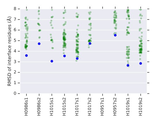
Fig. 12 | Accuracy of predictions for interfaces. For the five all-groups heterodimer CASP13 targets the full-atom RMSDs of the interface residues (residues with a ground truth inter-chain heavy atom distance $< 10$ Å) are computed for all groups’ chain submissions, relative to the target complex. Results $> 8$ Å are not shown. AlphaFold achieves consistently high accuracy interface regions and for 4 out of 5 targets predicts both chains’ interfaces below $< 5$ Å.

图 12｜界面预测的精度。对五个 all-groups 的 CASP13 异源二聚体靶标，计算所有队伍链提交中界面残基（真实结构里链间重原子距离 $< 10$ Å 的残基）相对于靶标复合物的全原子 RMSD。$> 8$ Å 的结果未画出。AlphaFold 在界面区域上始终达到较高精度，并在 5 个靶标中的 4 个上把两条链的界面都预测到 $< 5$ Å 以内。

Further evidence of AlphaFold reaching accuracy sufficient for biological relevance is shown in Figure 13. The images show the pocket in T1011 indicating that the accuracy gain in AlphaFold’s structure prediction can leads to more accurate prediction of pocket geometry and thus the binding of ligands.

图 13 给出了进一步证据，说明 AlphaFold 已达到足以具有生物学意义的精度。图中展示的是 T1011 中的口袋，表明 AlphaFold 结构预测精度的提高，可以带来对口袋几何以及因此对配体结合的更准确预测。

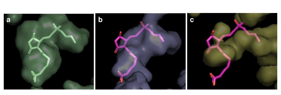
Fig. 13 | Ligand pocket visualizations for T1011 PDB 6M9T: EP3 receptor bound to misoprostol-FA$^{24}$ (a) the native structure showing the ligand in a pocket. (b) AlphaFold’s submission 5 (78.0 GDT TS) made without knowledge of the ligand shows a pocket more similar to the true pocket than that of (c) the best other submission (322 model 3, 68.7 GDT TS). Both submissions are aligned to the native using the same subset of residues from the helices close to the ligand pocket and visualized with the interior pocket together with the native ligand position.

图 13｜T1011（PDB 6M9T：与 misoprostol-FA 结合的 EP3 受体）$^{24}$ 的配体口袋可视化。(a) 天然结构，显示口袋中的配体。(b) AlphaFold 的第 5 次提交（78.0 GDT TS）在并不知道配体的情况下做出，其口袋比 (c) 其他队伍最好的提交（322 组模型 3，68.7 GDT TS）更接近真实口袋。两次提交都用靠近配体口袋的螺旋上同一组残基与天然结构对齐，并与内部口袋以及天然配体位置一起可视化。

So far only template-based predictions have been able to deliver the most accurate predictions. While AlphaFold is able to match template-based modelling without using templates, and in some cases outperform other methods (e.g. T0981-D5, 72.8 GDT TS, and T0957s1-D2, 88.0 GDT TS, two TBM-hard domains where AlphaFold’s top-1 model is 12 GDT TS better than any other top-1 submission) accuracy for FM targets still lags that for TBM targets and can still not be relied upon for detailed understanding of hard structures. In an analysis of the performance of CASP13 TBM predictions for Molecular Replacement, Read et al.$^{25}$ reported that the AlphaFold predictions (raw coordinates, without $B$-factors) led to a marginally greater log-likelihood gain (LLG) than those of any other group, indicating that these improved structures can assist in phasing for X-ray crystallography.

迄今只有基于模板的预测能够给出最准确的结果。虽然 AlphaFold 能够在不使用模板的情况下与模板建模相当，并在某些情形下超过其他方法（例如 T0981-D5，72.8 GDT TS，以及 T0957s1-D2，88.0 GDT TS；这两个 TBM-hard 结构域上，AlphaFold 的 top-1 模型比任何其他 top-1 提交高出 12 个 GDT TS），但 FM 靶标上的精度仍落后于 TBM 靶标，还不能用来可靠地细致理解困难结构。在一项关于 CASP13 TBM 预测用于分子置换的分析中，Read 等人$^{25}$ 报告，AlphaFold 的预测（原始坐标，不含 $B$ 因子）带来的对数似然增益（LLG）略高于任何其他队伍，表明这些改进后的结构可以帮助 X 射线晶体学中的相位确定。

Interpretation of distogram neural network We have shown that the deep distance prediction neural network achieves high accuracy, but we would like to understand how the network arrives at its distance predictions, and in particular to understand how the inputs to the model affect the final prediction. This might lead to understanding of the folding mechanisms or suggest improvements to the model. However, deep neural networks are complex non-linear functions of their inputs, and so this attribution problem is difficult, under-specified and an on-going topic of research. Even so, there are a number of methods for such analysis: here we apply Integrated Gradients [26] to our trained distogram network to indicate the location of input features which affect the network’s predictions of a particular distance.

对距离图神经网络的解释 我们已经表明，这个深层距离预测神经网络达到了很高的精度，但我们还希望理解网络是如何得到其距离预测的，尤其是模型的输入如何影响最终预测。这或许有助于理解折叠机制，或提示改进模型的途径。然而，深度神经网络是其输入的复杂非线性函数，因此这一归因问题很困难、也不充分确定，仍是正在研究的课题。尽管如此，已有若干方法可用于这类分析：这里我们对训练好的距离图网络应用积分梯度（Integrated Gradients）[26]，以标出影响网络对某一特定距离之预测的输入特征位置。

Given the expected value of the distance between any two residues $I$ and $J$, $d^{I,J}(x)$, we can consider its derivatives with respect to the input features $x_{i,j,c}$, where $i$ and $j$ are residue indices and $c$ is the feature channel index. The attribution function, as calculated using Integrated Gradients, of the expected distance between residues $I$ and $J$ with respect to the input features is then defined as

给定任意两个残基 $I$ 与 $J$ 之间距离的期望值 $d^{I,J}(x)$，我们可以考察它对输入特征 $x_{i,j,c}$ 的导数，其中 $i$ 和 $j$ 是残基索引，$c$ 是特征通道索引。用积分梯度计算的、残基 $I$ 与 $J$ 之间期望距离对输入特征的归因函数，于是定义为

$$S^{I,J}_{i,j,c} = (x_{i,j,c} - x'_c) \int_{\alpha=0}^{1} d\alpha\, \frac{\partial d^{I,J}(\alpha x + (1-\alpha)x')}{\partial x_{i,j,c}}, \tag{7}$$

$$\mathrm{s.t.}\ \sum_{i,j,c} S^{I,J}_{i,j,c} = d^{I,J}(x) - d^{I,J}(x'), \tag{8}$$

where $x'$ is a reference set of features; in this case we average the input features spatially:

其中 $x'$ 是一组参照特征；在这里我们对输入特征做空间平均：

$$x'_c = \frac{1}{N^2} \sum_{i=0,j=0}^{N,N} x_{i,j,c}. \tag{9}$$

The derivatives of $d$ can be calculated using backpropagation on the trained distogram network, and the integral over $\alpha$ is approximated as a numerical summation.

$d$ 的导数可以用训练好的距离图网络通过反向传播计算，对 $\alpha$ 的积分则近似为数值求和。

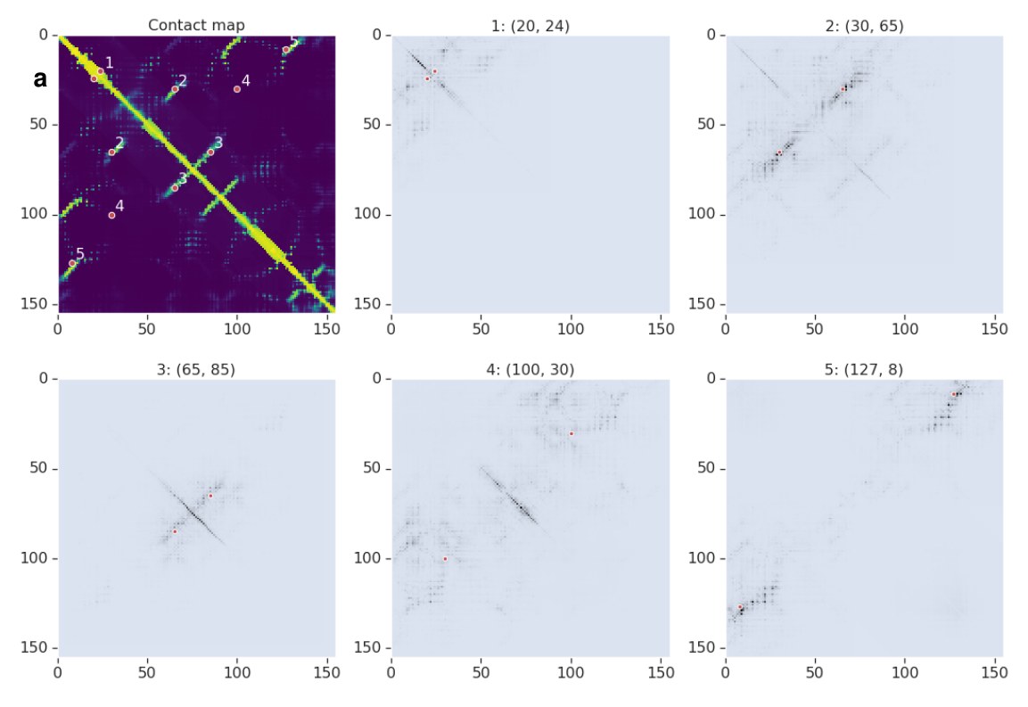
Fig. 14 | Attribution map of distogram network The contact probability map of T0986s2, and the summed absolute value of the Integrated Gradient, $\sum_c |S^{I,J}_{i,j,c}|$, of the input 2D features with respect to the expected distance between five different pairs of residues $(I, J)$: (1) a helix self-contact, (2) a long-range stand-strand contact, (3) a medium-range strand-strand contact, (4) a non-contact and (5) a very long-range strand-strand contact. Each pair is shown as two red dots on the diagrams. Darker means higher attribution weight.

图 14｜距离图网络的归因图。T0986s2 的接触概率图，以及输入二维特征相对于五对不同残基 $(I, J)$ 的期望距离的积分梯度绝对值之和 $\sum_c |S^{I,J}_{i,j,c}|$：(1) 螺旋自接触，(2) 长程折叠股–折叠股接触，(3) 中程折叠股–折叠股接触，(4) 非接触，以及 (5) 非常长程的折叠股–折叠股接触。每对在图中以两个红点标出。颜色越深表示归因权重越高。

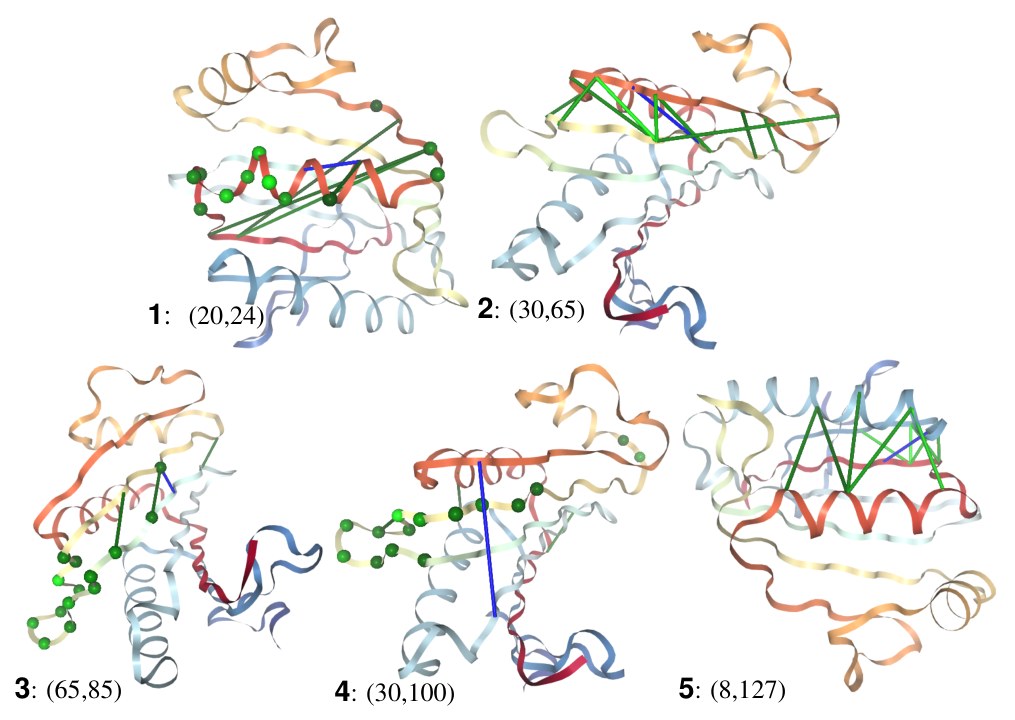
Fig. 15 | Attribution shown on predicted structure. For T0986s2 (TM-score 0.8), the top 10 input pairs, including self-pairs, with highest attribution weight for each of the five output pairs shown in Figure 14, are shown as lines (or spheres, for self-pairs) coloured by sensitivity, lighter green is more sensitive, and the output pair shown as a blue line.

图 15｜在预测结构上显示的归因。对 T0986s2（TM-score 0.8），就图 14 中所示五对输出中的每一对，把归因权重最高的前 10 个输入对（包括自身对）画成线段（自身对则画成球），颜色表示敏感度，较浅的绿色更敏感；输出对画成蓝线。

In Figure 14, plots of summed absolute Integrated Gradient, $\sum_c |S^{I,J}_{i,j,c}|$, are shown for selected $I, J$ output pairs in T0986s2 and in Figure 15, the top-10 highest attribution input pairs for each output pair are shown on top of AlphaFold’s top-1 predicted structure. The attribution maps are sparse and highly structured, closely reflecting the predicted geometry of the protein. For the four in-contact pairs presented (1, 2, 3, 5), all the highest attribution pairs are pairs within or between the secondary structure that one or both the output pair are members of. In (1) the helix residues are important as well as connections between the strands which follow either end of the helix, which might indicate strain on the helix. In (2) all the most important residue pairs connect the same two strands, whereas in (3) a mix of inter-strand pairs and strand residues are most salient. In (5) the most important pairs involve the packing of nearby secondary structure elements to the strand and helix. For the non-contacting pair (4), the most important input pairs are the residues that are geometrically between $I$ and $J$ in the predicted protein structure. Furthermore, most of the high attribution input pairs are themselves in contact.

图 14 给出了 T0986s2 中选定输出对 $I, J$ 的积分梯度绝对值之和 $\sum_c |S^{I,J}_{i,j,c}|$；图 15 则把每对输出归因最高的前 10 个输入对，画在 AlphaFold 的 top-1 预测结构上。这些归因图稀疏且结构性强，密切反映了蛋白质的预测几何。对所展示的四对接触（1、2、3、5），归因最高的对都位于输出对一方或双方所属二级结构的内部或之间。在 (1) 中，螺旋残基很重要，螺旋两端随后折叠股之间的连接也很重要，这可能表明螺旋受到应变。在 (2) 中，最重要的残基对都连接着同一对折叠股；而在 (3) 中，最显著的则是股间残基对与折叠股残基的混合。在 (5) 中，最重要的对涉及附近二级结构元件向该折叠股和螺旋的堆积。对非接触对 (4)，最重要的输入对是在预测蛋白质结构里几何上位于 $I$ 与 $J$ 之间的残基。此外，大多数高归因输入对本身也处于接触。

Since the network is tasked with predicting the spatial geometry, with no structure available at the input, these patterns of interaction indicate that the network is using intermediate predictions to discover important interactions and channelling information from related residues to refine the final prediction.

由于网络的任务是在输入端没有结构的情况下预测空间几何，这些相互作用模式表明，网络正在利用中间预测去发现重要的相互作用，并把相关残基的信息汇集起来，以改进最终预测。

References

参考文献

1. Gilliland, G. et al. The Protein Data Bank. Nucleic Acids Res. 28, 235–242 (2000).

2. Dawt1son, N. et al. CATH: An expanded resource to predict protein function through structure and sequence. Nucleic Acids Res. (2017).

3. Mirdita, M. et al. Uniclust databases of clustered and deeply annotated protein sequences and alignments. Nucleic Acids Res. 45, D170–D176 (2016).

4. Remmert, M., Biegert, A., Hauser, A. & Söding, J. HHblits: lightning-fast iterative protein sequence searching by HMM-HMM alignment. Nature Methods 9, 173 (2012).

5. Seemayer, S., Gruber, M. & Söding, J. CCMpred—fast and precise prediction of protein residue–residue contacts from correlated mutations. Bioinformatics 30, 3128–3130 (2014).

6. Altschul, S. F. et al. Gapped BLAST and PSI-BLAST: a new generation of protein database search programs. Nucleic Acids Res. 25, 3389–3402 (1997).

7. Wang, S., Sun, S., Li, Z., Zhang, R. & Xu, J. Accurate De Novo Prediction of Protein Contact Map by Ultra-Deep Learning Model. PLoS Comput. Biol. 13, 999–1006 (2017).

8. He, K., Zhang, X., Ren, S. & Sun, J. Deep Residual Learning for Image Recognition. arXiv preprint arXiv:1512.03385 abs/1512.03385 (2015).

9. Yu, F. & Koltun, V. Multi-scale context aggregation by dilated convolutions. arXiv preprint arXiv:1511.07122 (2015).

10. Oord, A. v. d. et al. Wavenet: A generative model for raw audio. arXiv preprint arXiv:1609.03499 (2016).

11. Clevert, D.-A., Unterthiner, T. & Hochreiter, S. Fast and Accurate Deep Network Learning by Exponential Linear Units (ELUs). arXiv preprint arXiv:1511.07289 (2015).

12. Jones, D. T. & Kandathil, S. M. High precision in protein contact prediction using fully convolutional neural networks and minimal sequence features. Bioinformatics 1, 8 (2018).

13. Kabsch, W. & Sander, C. Dictionary of protein secondary structure: pattern recognition of hydrogen-bonded and geometrical features. Biopolymers 22, 2577–2637 (1983).

14. Yang, Y. et al. Sixty-five years of the long march in protein secondary structure prediction: the final stretch? Briefings Bioinf. 19, 482–494. ISSN: 1467-5463 (2016).

15. Jones, D., Singh, T., Kosciolek, T. & Tetchner, S. MetaPSICOV: Combining coevolution methods for accurate prediction of contacts and long range hydrogen bonding in proteins. Bioinformatics 31, 999–1006 (2015).

16. Liu, D. C. & Nocedal, J. On the limited memory BFGS method for large scale optimization. Math. Program. 45, 503–528 (1989).

17. Zemla, A., Venclovas, C., Moult, J. & Fidelis, K. Processing and analysis of CASP3 protein structure predictions. Proteins 37, 22–29 (1999).

18. Mariani, V., Biasini, M., Barbato, A. & Schwede, T. lDDT: a local superposition-free score for comparing protein structures and models using distance difference tests. Bioinformatics 29, 2722–2728 (2013).

19. Söding, J., Biegert, A. & Lupas, A. The HHpred interactive server for protein homology detection and structure prediction. Nucleic acids research 33, W244–W248 (2005).

20. Cong, Q. et al. An automatic method for CASP9 free modeling structure prediction assessment. Bioinformatics 27, 3371–3378 (2011).

21. Kayikci, M. et al. Protein contacts atlas: visualization and analysis of non-covalent contacts in biomolecules. Nat. Struct. Mol. Biol. 25, 185–194 (2018).

22. Zhang, Y. & Skolnick, J. TM-align: A protein structure alignment algorithm based on TM-score. Nucleic Acids Research 33, 2302–2309 (2005).

23. Tovchigrechko, A., Wells, C. & Vakser, I. Docking of protein models. Protein Sci. 11, 1888–1896 (2002).

24. Audet, M. et al. Crystal structure of misoprostol bound to the labor inducer prostaglandin E$_2$ receptor. Nature chemical biology 15, 11 (2019).

25. Read, R. Molecular replacement in CASP13. In preparation (2019).

26. Sundararajan, M., Taly, A. & Yan, Q. Axiomatic Attribution for Deep Networks. CoRR abs/1703.01365 (2017).

2 Acknowledgements

2 致谢

We thank Clemens Meyer for assistance in preparing the paper; Ben Coppin, Oriol Vinyals, Marek Barwinski, Ruoxi Sun, Carl Elkin, Peter Dolan, Matthew Lai and Yujia Li for their contributions and support; Olaf Ronneberger for reviewing the paper; the rest of the DeepMind team for their support; the CASP13 organisers and the experimentalists whose structures enabled the assessment.

我们感谢 Clemens Meyer 协助准备本文；感谢 Ben Coppin、Oriol Vinyals、Marek Barwinski、Ruoxi Sun、Carl Elkin、Peter Dolan、Matthew Lai 和 Yujia Li 的贡献与支持；感谢 Olaf Ronneberger 审阅本文；感谢 DeepMind 团队其他成员的支持；并感谢 CASP13 组织者以及以其实验结构使本次评估成为可能的实验工作者。

3 Author contributions

3 作者贡献

R.E., J.J., J.K., L.S., A.S., C.Q., T.G., A.Z., A.B., H.P. and K.S. designed and built the AlphaFold system with advice from D.S., K.K. and D.H..

R.E.、J.J.、J.K.、L.S.、A.S.、C.Q.、T.G.、A.Z.、A.B.、H.P. 和 K.S. 设计并构建了 AlphaFold 系统，D.S.、K.K. 和 D.H. 提供了建议。

D.J. provided advice and guidance on protein structure prediction methodology.

D.J. 就蛋白质结构预测方法提供了建议与指导。

S.P. contributed to software engineering.

S.P. 参与了软件工程工作。

S.C., A.N., K.K. and D.H. managed the project.

S.C.、A.N.、K.K. 和 D.H. 负责项目管理。

J.K., A.S., T.G., A.Z., A.B., R.E., P.K. and J.J. analysed the CASP results for the paper.

J.K.、A.S.、T.G.、A.Z.、A.B.、R.E.、P.K. 和 J.J. 为本文分析了 CASP 结果。

A.S., J.K. wrote the paper with contributions from J.J, R.E., L.S., T.G., A.Z., D.J., P.K., K.K. and D.H.

A.S.、J.K. 撰写了本文，J.J、R.E.、L.S.、T.G.、A.Z.、D.J.、P.K.、K.K. 和 D.H. 亦有贡献。

A.S. led the team.

A.S. 领导了该团队。

4 Competing financial interests

4 竞争性经济利益

A.S., J.K., L.S., R.E., H.P., C.Q., K.S. and J.J. have filed provisional patent application 62/734,757. A.S. and J.J. have filed provisional patent application 62/734,773. A.S., J.K., T.G., J.J. L.S., R.E. and C.Q. have filed provisional patent application 62/770,490. J.J., A.S., R.E., A.B., T.G. and A.Z. have filed provisional patent application 62/774,071. The remaining authors declare no competing financial interests.

A.S.、J.K.、L.S.、R.E.、H.P.、C.Q.、K.S. 和 J.J. 已提交临时专利申请 62/734,757。A.S. 和 J.J. 已提交临时专利申请 62/734,773。A.S.、J.K.、T.G.、J.J. L.S.、R.E. 和 C.Q. 已提交临时专利申请 62/770,490。J.J.、A.S.、R.E.、A.B.、T.G. 和 A.Z. 已提交临时专利申请 62/774,071。其余作者声明不存在竞争性经济利益。

5 Materials and correspondence

5 材料与通信

Correspondence and materials requests should be sent to Andrew Senior: andrewsenior@google.com

6 Reporting summary

6 报告摘要

Further information on experimental design is available in the Nature Research Reporting Summary linked to this article.

有关实验设计的进一步信息，见本文链接的 Nature Research Reporting Summary。

7 Code availability

7 代码可用性

Upon publication we will make available source code for the distogram and torsion predictions, together with neural network weights and input data for the CASP13 targets.

发表后，我们将公开距离图与扭角预测的源代码，以及神经网络权重和 CASP13 靶标的输入数据。

We make use of several open-source libraries to conduct our experiments, particularly HHblits$^1$, PSI-BLAST$^2$ and the machine learning framework TensorFlow$^\S$ along with the TensorFlow library Sonnet$^\P$ which provides implementations of individual model components$^3$. We also used Rosetta$^4$ under license.

我们的实验使用了若干开源库，尤其是 HHblits$^1$、PSI-BLAST$^2$，以及机器学习框架 TensorFlow$^\S$ 和提供各个模型组件实现的 TensorFlow 库 Sonnet$^\P$$^3$。我们还在许可下使用了 Rosetta$^4$。

$^\S$https://github.com/tensorflow/tensorflow

$^\P$https://github.com/deepmind/sonnet

8 Data availability

8 数据可用性

The following public datasets were used in this work:

本工作使用了下列公开数据集：

• PDB 2018-03-15

• CATH 2018-03-16

• Uniclust30 2017-10

• PSI-BLAST nr dataset (as of 2017-12-15)

• PSI-BLAST nr 数据集（截至 2017-12-15）

We will make available our train/test split (CATH domain codes).

我们将公开我们的训练/测试划分（CATH 结构域编码）。

9 Extended data

9 扩展数据

The following tools and data set versions were used for the CASP system and for subsequent experiments.

CASP 系统以及随后的实验使用了下列工具和数据集版本。

• PDB 2018-03-15

• CATH 2018-03-16

• HHblits based on version 3.0-beta.3 (3 iterations, E-value 1e-3)

• 基于 3.0-beta.3 版的 HHblits（3 次迭代，E-value 1e-3）

• HHpred web server

• HHpred 网页服务器

• Uniclust30 2017-10

• PSI-BLAST version 2.6.0 nr dataset (as of 2017-12-15) (3 iterations, E-value 1e-3)

• PSI-BLAST 2.6.0 版 nr 数据集（截至 2017-12-15）（3 次迭代，E-value 1e-3）

• SST web server (March 2019)

• SST 网页服务器（2019 年 3 月）

• BioPython v1.65

• Rosetta v3.5

• PyMol for structure visualisation.

• 用于结构可视化的 PyMol。

• TM-align 20160521