Asynchronous Methods for Deep Reinforcement Learning
Asynchronous Methods for Deep Reinforcement Learning
Volodymyr Mnih 1 Adrià Puigdomènech Badia 1 Mehdi Mirza 1,2 Alex Graves 1 Tim Harley 1 Timothy P. Lillicrap 1 David Silver 1 Koray Kavukcuoglu 1 Address: 1 Google DeepMind 2 Montreal Institute for Learning Algorithms (MILA), University of Montreal
Supplementary Material for "Asynchronous Methods for Deep Reinforcement Learning"
「Asynchronous Methods for Deep Reinforcement Learning」补充材料
Volodymyr Mnih 1 Adrià Puigdomènech Badia 1 Mehdi Mirza 1,2 Alex Graves 1 Tim Harley 1 Timothy P. Lillicrap 1 David Silver 1 Koray Kavukcuoglu 1 Address: 1 Google DeepMind 2 Montreal Institute for Learning Algorithms (MILA), University of Montreal
Abstract
摘要
We propose a conceptually simple and lightweight framework for deep reinforcement learning that uses asynchronous gradient descent for optimization of deep neural network controllers. We present asynchronous variants of four standard reinforcement learning algorithms and show that parallel actor-learners have a stabilizing effect on training allowing all four methods to successfully train neural network controllers. The best performing method, an asynchronous variant of actor-critic, surpasses the current state-of-the-art on the Atari domain while training for half the time on a single multi-core CPU instead of a GPU. Furthermore, we show that asynchronous actor-critic succeeds on a wide variety of continuous motor control problems as well as on a new task of navigating random 3D mazes using a visual input.
我们提出一个概念上简单且轻量的深度强化学习框架,用异步梯度下降优化深度神经网络控制器。我们给出四种标准强化学习算法的异步变体,并表明并行 actor-learner 对训练有稳定作用,使四种方法都能成功训练神经网络控制器。表现最好的方法——actor-critic 的异步变体——在 Atari 领域超过当时最优,却只需在单台多核 CPU 上训练一半时间,而非 GPU。此外,我们表明异步 actor-critic 在多种连续电机控制问题上也成功,并在仅用视觉输入导航随机 3D 迷宫的新任务上成功。
1 Introduction
1 引言
Deep neural networks provide rich representations that can enable reinforcement learning (RL) algorithms to perform effectively. However, it was previously thought that the combination of simple online RL algorithms with deep neural networks was fundamentally unstable. Instead, a variety of solutions have been proposed to stabilize the algorithm (Riedmiller 2005; Mnih et al. 2013; Mnih et al. 2015; Van Hasselt et al. 2015; Schulman et al. 2015a). These approaches share a common idea: the sequence of observed data encountered by an online RL agent is non-stationary, and online RL updates are strongly correlated. By storing the agent’s data in an experience replay memory, the data can be batched (Riedmiller 2005; Schulman et al. 2015a) or randomly sampled (Mnih et al. 2013; Mnih et al. 2015; Van Hasselt et al. 2015) from different time-steps. Aggregating over memory in this way reduces non-stationarity and decorrelates updates, but at the same time limits the methods to off-policy reinforcement learning algorithms.
深度神经网络提供丰富表示,可使强化学习(RL)算法有效运行。但此前人们认为,简单在线 RL 算法与深度神经网络的组合本质上不稳定。于是提出了多种稳定算法的方案(Riedmiller 2005;Mnih et al. 2013;Mnih et al. 2015;Van Hasselt et al. 2015;Schulman et al. 2015a)。这些做法共享一个想法:在线 RL 智能体遇到的观测数据序列非平稳,且在线 RL 更新强相关。通过把智能体数据存入经验回放内存,数据可批处理(Riedmiller 2005;Schulman et al. 2015a)或从不同时间步随机采样(Mnih et al. 2013;Mnih et al. 2015;Van Hasselt et al. 2015)。如此在内存上聚合可降低非平稳性并去相关更新,但同时也把方法限制在离策略强化学习算法上。
Deep RL algorithms based on experience replay have achieved unprecedented success in challenging domains such as Atari 2600. However, experience replay has several drawbacks: it uses more memory and computation per real interaction; and it requires off-policy learning algorithms that can update from data generated by an older policy.
基于经验回放的深度 RL 算法在 Atari 2600 等挑战性领域取得前所未有的成功。但经验回放有若干缺点:每次真实交互消耗更多内存与计算;且需要能从更旧策略生成的数据中更新的离策略学习算法。
In this paper we provide a very different paradigm for deep reinforcement learning. Instead of experience replay, we asynchronously execute multiple agents in parallel, on multiple instances of the environment. This parallelism also decorrelates the agents’ data into a more stationary process, since at any given time-step the parallel agents will be experiencing a variety of different states. This simple idea enables a much larger spectrum of fundamental on-policy RL algorithms, such as Sarsa, n-step methods, and actor-critic methods, as well as off-policy RL algorithms such as Q-learning, to be applied robustly and effectively using deep neural networks.
本文提供一种截然不同的深度强化学习范式。我们不用经验回放,而是在环境的多个实例上并行异步执行多个智能体。这种并行也把智能体数据去相关成更平稳的过程,因为在任意给定时间步,并行智能体将经历多种不同状态。这一简单想法使更广谱的基本在策略 RL 算法——如 Sarsa、n-step 方法与 actor-critic 方法——以及 Q-learning 等离策略 RL 算法,都能用深度神经网络稳健有效地应用。
Our parallel reinforcement learning paradigm also offers practical benefits. Whereas previous approaches to deep reinforcement learning rely heavily on specialized hardware such as GPUs (Mnih et al. 2015; Van Hasselt et al. 2015; Schaul et al. 2015) or massively distributed architectures (Nair et al. 2015), our experiments run on a single machine with a standard multi-core CPU. When applied to a variety of Atari 2600 domains, on many games asynchronous reinforcement learning achieves better results, in far less time than previous GPU-based algorithms, using far less resource than massively distributed approaches. The best of the proposed methods, asynchronous advantage actor-critic (A3C), also mastered a variety of continuous motor control tasks as well as learned general strategies for exploring 3D mazes purely from visual inputs. We believe that the success of A3C on both 2D and 3D games, discrete and continuous action spaces, as well as its ability to train feedforward and recurrent agents makes it the most general and successful reinforcement learning agent to date.
我们的并行强化学习范式还有实践益处。先前深度强化学习做法严重依赖 GPU 等专用硬件(Mnih et al. 2015;Van Hasselt et al. 2015;Schaul et al. 2015)或大规模分布式架构(Nair et al. 2015),而我们的实验在配备标准多核 CPU 的单机上运行。应用于多种 Atari 2600 领域时,异步强化学习在许多游戏上以远少于先前基于 GPU 算法的时间、远少于大规模分布式做法的资源取得更好结果。所提方法中最好的异步优势 actor-critic(A3C)还掌握了多种连续电机控制任务,并仅从视觉输入学到探索 3D 迷宫的一般策略。我们相信,A3C 在 2D 与 3D 游戏、离散与连续动作空间上的成功,以及训练前馈与循环智能体的能力,使其成为迄今最通用、最成功的强化学习智能体。
2 Related Work
2 相关工作
The General Reinforcement Learning Architecture (Gorila) of (Nair et al. 2015) performs asynchronous training of reinforcement learning agents in a distributed setting. In Gorila, each process contains an actor that acts in its own copy of the environment, a separate replay memory, and a learner that samples data from the replay memory and computes gradients of the DQN loss (Mnih et al. 2015) with respect to the policy parameters. The gradients are asynchronously sent to a central parameter server which updates a central copy of the model. The updated policy parameters are sent to the actor-learners at fixed intervals. By using 100 separate actor-learner processes and 30 parameter server instances, a total of 130 machines, Gorila was able to significantly outperform DQN over 49 Atari games. On many games Gorila reached the score achieved by DQN over 20 times faster than DQN. We also note that a similar way of parallelizing DQN was proposed by (Chavez et al. 2015).
(Nair et al. 2015)的通用强化学习架构(Gorila)在分布式设定下做强化学习智能体的异步训练。在 Gorila 中,每个进程包含在自己环境副本中行动的 actor、单独的回放内存,以及从回放内存采样数据并相对策略参数计算 DQN 损失(Mnih et al. 2015)梯度的 learner。梯度被异步发送到更新模型中心副本的中央参数服务器。更新后的策略参数按固定间隔发给 actor-learner。通过使用 100 个独立 actor-learner 进程与 30 个参数服务器实例、共 130 台机器,Gorila 能在 49 个 Atari 游戏上显著超过 DQN。在许多游戏上 Gorila 达到 DQN 分数的速度比 DQN 快超过 20 倍。我们也指出,(Chavez et al. 2015)提出过类似的并行化 DQN 方式。
In earlier work, (Li & Schuurmans 2011) applied the Map Reduce framework to parallelizing batch reinforcement learning methods with linear function approximation. Parallelism was used to speed up large matrix operations but not to parallelize the collection of experience or stabilize learning. (Grounds & Kudenko 2008) proposed a parallel version of the Sarsa algorithm that uses multiple separate actor-learners to accelerate training. Each actor-learner learns separately and periodically sends updates to weights that have changed significantly to the other learners using peer-to-peer communication.
更早的工作中,(Li & Schuurmans 2011)把 MapReduce 框架用于并行化带线性函数逼近的批量强化学习方法。并行用于加速大矩阵运算,而非并行化经验收集或稳定学习。(Grounds & Kudenko 2008)提出使用多个独立 actor-learner 加速训练的并行版 Sarsa 算法。每个 actor-learner 单独学习,并周期性地用点对点通信把显著变化的权重更新发给其他 learner。
(Tsitsiklis 1994) studied convergence properties of Q-learning in the asynchronous optimization setting. These results show that Q-learning is still guaranteed to converge when some of the information is outdated as long as outdated information is always eventually discarded and several other technical assumptions are satisfied. Even earlier, (Bertsekas 1982) studied the related problem of distributed dynamic programming.
(Tsitsiklis 1994)研究了异步优化设定下 Q-learning 的收敛性质。这些结果表明:只要过时信息最终总被丢弃且满足若干其他技术假设,即使部分信息过时,Q-learning 仍保证收敛。更早地,(Bertsekas 1982)研究了相关的分布式动态规划问题。
Another related area of work is in evolutionary methods, which are often straightforward to parallelize by distributing fitness evaluations over multiple machines or threads (Tomassini 1999). Such parallel evolutionary approaches have recently been applied to some visual reinforcement learning tasks. In one example, (Koutník et al. 2014) evolved convolutional neural network controllers for the TORCS driving simulator by performing fitness evaluations on 8 CPU cores in parallel.
另一相关领域是演化方法,常可通过把适应度评估分布到多台机器或多线程上直接并行化(Tomassini 1999)。此类并行演化做法最近被用于一些视觉强化学习任务。例如,(Koutník et al. 2014)通过在 8 个 CPU 核上并行做适应度评估,为 TORCS 驾驶模拟器演化卷积神经网络控制器。
3 Reinforcement Learning Background
3 强化学习背景
We consider the standard reinforcement learning setting where an agent interacts with an environment over a number of discrete time steps. At each time step , the agent receives a state and selects an action from some set of possible actions according to its policy , where is a mapping from states to actions . In return, the agent receives the next state and receives a scalar reward . The process continues until the agent reaches a terminal state after which the process restarts. The return is the total accumulated return from time step with discount factor . The goal of the agent is to maximize the expected return from each state .
我们考虑标准强化学习设定:智能体在若干离散时间步上与环境 交互。在每个时间步 ,智能体收到状态 ,并根据其策略 从可能动作集合 中选择动作 ,其中 是从状态 到动作 的映射。作为回报,智能体收到下一状态 与标量奖励 。过程持续到智能体到达终止状态,之后过程重启。回报 是从时间步 起、折扣因子为 的总累积回报。智能体的目标是最大化每个状态 的期望回报。
The action value is the expected return for selecting action in state and following policy . The optimal value function gives the maximum action value for state and action achievable by any policy. Similarly, the value of state under policy is defined as and is simply the expected return for following policy from state .
动作价值 是在状态 选择动作 并遵循策略 的期望回报。最优价值函数 给出任何策略在状态 、动作 上可达到的最大动作价值。类似地,策略 下状态 的价值定义为 ,即从状态 遵循策略 的期望回报。
In value-based model-free reinforcement learning methods, the action value function is represented using a function approximator, such as a neural network. Let be an approximate action-value function with parameters . The updates to can be derived from a variety of reinforcement learning algorithms. One example of such an algorithm is Q-learning, which aims to directly approximate the optimal action value function: . In one-step Q-learning, the parameters of the action value function are learned by iteratively minimizing a sequence of loss functions, where the th loss function defined as
在基于价值的无模型强化学习方法中,动作价值函数用函数逼近器(如神经网络)表示。设 为带参数 的近似动作价值函数。对 的更新可从多种强化学习算法导出。此类算法的一个例子是 Q-learning,它旨在直接逼近最优动作价值函数:。在一步 Q-learning 中,动作价值函数 的参数 通过迭代最小化一系列损失函数来学习,其中第 个损失函数定义为
where is the state encountered after state .
其中 是状态 之后遇到的状态。
We refer to the above method as one-step Q-learning because it updates the action value toward the one-step return . One drawback of using one-step methods is that obtaining a reward only directly affects the value of the state action pair that led to the reward. The values of other state action pairs are affected only indirectly through the updated value . This can make the learning process slow since many updates are required the propagate a reward to the relevant preceding states and actions.
我们称上述方法为一步 Q-learning,因为它把动作价值 朝一步回报 更新。使用一步方法的一个缺点是:获得奖励 只直接影响到导致该奖励的状态动作对 的价值。其他状态动作对的价值仅通过更新后的 间接受影响。这可能使学习过程变慢,因为需要许多更新才能把奖励传播到相关的先前状态与动作。
One way of propagating rewards faster is by using -step returns (Watkins 1989; Peng & Williams 1996). In -step Q-learning, is updated toward the -step return defined as . This results in a single reward directly affecting the values of preceding state action pairs. This makes the process of propagating rewards to relevant state-action pairs potentially much more efficient.
更快传播奖励的一种方式是使用 -step 回报(Watkins 1989;Peng & Williams 1996)。在 -step Q-learning 中, 朝定义为 的 -step 回报更新。这使单个奖励 直接影响 个先前状态动作对的价值,从而使把奖励传播到相关状态–动作对的过程潜在地高效得多。
In contrast to value-based methods, policy-based model-free methods directly parameterize the policy and update the parameters by performing, typically approximate, gradient ascent on . One example of such a method is the REINFORCE family of algorithms due to Williams (Williams 1992). Standard REINFORCE updates the policy parameters in the direction , which is an unbiased estimate of . It is possible to reduce the variance of this estimate while keeping it unbiased by subtracting a learned function of the state , known as a baseline (Williams 1992), from the return. The resulting gradient is .
与基于价值的方法相对,基于策略的无模型方法直接参数化策略 ,并通过(通常近似的)对 做梯度上升来更新参数 。此类方法的一个例子是 Williams 的 REINFORCE 族算法(Williams 1992)。标准 REINFORCE 沿 方向更新策略参数 ,这是 的无偏估计。可通过从回报中减去状态的学习函数 (称为基线,Williams 1992)来降低该估计的方差并保持无偏。所得梯度为 。
A learned estimate of the value function is commonly used as the baseline leading to a much lower variance estimate of the policy gradient. When an approximate value function is used as the baseline, the quantity used to scale the policy gradient can be seen as an estimate of the advantage of action in state , or , because is an estimate of and is an estimate of . This approach can be viewed as an actor-critic architecture where the policy is the actor and the baseline is the critic (Sutton & Barto 1998; Degris et al. 2012).
价值函数的学习估计常被用作基线 ,从而得到方差低得多的策略梯度估计。当用近似价值函数作基线时,用于缩放策略梯度的量 可视为动作 在状态 上的优势估计,即 ,因为 是 的估计, 是 的估计。这一做法可视为 actor-critic 架构:策略 是 actor,基线 是 critic(Sutton & Barto 1998;Degris et al. 2012)。
4 Asynchronous RL Framework
4 异步 RL 框架
We now present multi-threaded asynchronous variants of one-step Sarsa, one-step Q-learning, n-step Q-learning, and advantage actor-critic. The aim in designing these methods was to find RL algorithms that can train deep neural network policies reliably and without large resource requirements. While the underlying RL methods are quite different, with actor-critic being an on-policy policy search method and Q-learning being an off-policy value-based method, we use two main ideas to make all four algorithms practical given our design goal.
我们现在给出一步 Sarsa、一步 Q-learning、n-step Q-learning 与优势 actor-critic 的多线程异步变体。设计这些方法的目标,是找到能可靠训练深度神经网络策略、且不要求大量资源的 RL 算法。尽管底层 RL 方法相当不同——actor-critic 是在策略的策略搜索方法,Q-learning 是离策略的基于价值方法——我们用两个主要想法,使四种算法在设计目标下都可实用。
First, we use asynchronous actor-learners, similarly to the Gorila framework (Nair et al. 2015), but instead of using separate machines and a parameter server, we use multiple CPU threads on a single machine. Keeping the learners on a single machine removes the communication costs of sending gradients and parameters and enables us to use Hogwild! (Recht et al. 2011) style updates for training.
第一,我们使用异步 actor-learner,类似 Gorila 框架(Nair et al. 2015),但不使用独立机器与参数服务器,而是在单机上使用多个 CPU 线程。把 learner 保持在单机上消除了发送梯度与参数的通信成本,并使我们能用 Hogwild!(Recht et al. 2011)风格的更新来训练。
Second, we make the observation that multiple actors-learners running in parallel are likely to be exploring different parts of the environment. Moreover, one can explicitly use different exploration policies in each actor-learner to maximize this diversity. By running different exploration policies in different threads, the overall changes being made to the parameters by multiple actor-learners applying online updates in parallel are likely to be less correlated in time than a single agent applying online updates. Hence, we do not use a replay memory and rely on parallel actors employing different exploration policies to perform the stabilizing role undertaken by experience replay in the DQN training algorithm.
第二,我们观察到:并行运行的多个 actor-learner 很可能在探索环境的不同部分。而且,可在每个 actor-learner 中显式使用不同探索策略以最大化这种多样性。通过在不同线程中运行不同探索策略,多个 actor-learner 并行施加在线更新对参数造成的总体变化,在时间上很可能比单个智能体施加在线更新更不相关。因此,我们不使用回放内存,而依赖采用不同探索策略的并行 actor 来承担 DQN 训练算法中经验回放所起的稳定作用。
In addition to stabilizing learning, using multiple parallel actor-learners has multiple practical benefits. First, we obtain a reduction in training time that is roughly linear in the number of parallel actor-learners. Second, since we no longer rely on experience replay for stabilizing learning we are able to use on-policy reinforcement learning methods such as Sarsa and actor-critic to train neural networks in a stable way. We now describe our variants of one-step Q-learning, one-step Sarsa, n-step Q-learning and advantage actor-critic.
除稳定学习外,使用多个并行 actor-learner 还有多项实践益处。第一,我们获得大致与并行 actor-learner 数量成线性的训练时间缩减。第二,由于不再依赖经验回放来稳定学习,我们能够用 Sarsa 与 actor-critic 等在策略强化学习方法以稳定方式训练神经网络。我们现在描述一步 Q-learning、一步 Sarsa、n-step Q-learning 与优势 actor-critic 的变体。
// Assume global shared , , and counter .
Initialize thread step counter
Initialize target network weights
Initialize network gradients
Get initial state
repeat
Take action with -greedy policy based on
Receive new state and reward
y=\left\{\begin{array}[]{l l}r&\text{for terminal }s^{\prime}\\ r+\gamma\max_{a^{\prime}}Q(s^{\prime},a^{\prime};\theta^{-})&\text{for non-terminal }s^{\prime}\end{array}\right.
Accumulate gradients wrt :
and
if then
Update the target network
end if
if or is terminal then
Perform asynchronous update of using .
Clear gradients .
end if
until
Algorithm 1 Asynchronous one-step Q-learning - pseudocode for each actor-learner thread.
// 假设全局共享 , , and counter .
Initialize thread step counter
Initialize target network weights
Initialize network gradients
Get initial state
repeat
Take action with -greedy policy based on
Receive new state and reward
y=\left\{\begin{array}[]{l l}r&\text{for terminal }s^{\prime}\\ r+\gamma\max_{a^{\prime}}Q(s^{\prime},a^{\prime};\theta^{-})&\text{for non-terminal }s^{\prime}\end{array}\right.
Accumulate gradients wrt :
and
if then
Update the target network
end if
if or is terminal then
Perform asynchronous update of using .
Clear gradients .
end if
until
算法 1 异步一步 Q-learning——每个 actor-learner 线程的伪代码。
Asynchronous one-step Q-learning: Pseudocode for our variant of Q-learning, which we call Asynchronous one-step Q-learning, is shown in Algorithm 1. Each thread interacts with its own copy of the environment and at each step computes a gradient of the Q-learning loss. We use a shared and slowly changing target network in computing the Q-learning loss, as was proposed in the DQN training method. We also accumulate gradients over multiple timesteps before they are applied, which is similar to using minibatches. This reduces the chances of multiple actor learners overwriting each other’s updates. Accumulating updates over several steps also provides some ability to trade off computational efficiency for data efficiency.
异步一步 Q-learning: 我们称为异步一步 Q-learning 的 Q-learning 变体伪代码见算法 1。每个线程与自己的环境副本交互,并在每步计算 Q-learning 损失的梯度。我们在计算 Q-learning 损失时使用共享且缓慢变化的目标网络,如 DQN 训练方法所提出。我们还在应用梯度前在多个时间步上累积梯度,这类似于使用 minibatch。这降低了多个 actor-learner 互相覆盖更新的机会。在若干步上累积更新也提供了在计算效率与数据效率之间折中的一定能力。
Finally, we found that giving each thread a different exploration policy helps improve robustness. Adding diversity to exploration in this manner also generally improves performance through better exploration. While there are many possible ways of making the exploration policies differ we experiment with using -greedy exploration with periodically sampled from some distribution by each thread.
最后,我们发现给每个线程不同的探索策略有助于提升稳健性。以这种方式增加探索多样性,一般也通过更好探索提升表现。虽有许多使探索策略不同的可能方式,我们实验用 -greedy 探索,并由每个线程周期性地从某分布采样 。
Asynchronous one-step Sarsa: The asynchronous one-step Sarsa algorithm is the same as asynchronous one-step Q-learning as given in Algorithm 1 except that it uses a different target value for . The target value used by one-step Sarsa is where is the action taken in state (Rummery & Niranjan 1994; Sutton & Barto 1998). We again use a target network and updates accumulated over multiple timesteps to stabilize learning.
异步一步 Sarsa: 异步一步 Sarsa 算法与算法 1 给出的异步一步 Q-learning 相同,只是对 使用不同的目标值。一步 Sarsa 使用的目标值为 ,其中 是在状态 采取的动作(Rummery & Niranjan 1994;Sutton & Barto 1998)。我们再次使用目标网络与在多个时间步上累积的更新来稳定学习。
Asynchronous n-step Q-learning: Pseudocode for our variant of multi-step Q-learning is shown in Supplementary Algorithm S2. The algorithm is somewhat unusual because it operates in the forward view by explicitly computing n-step returns, as opposed to the more common backward view used by techniques like eligibility traces (Sutton & Barto 1998). We found that using the forward view is easier when training neural networks with momentum-based methods and backpropagation through time. In order to compute a single update, the algorithm first selects actions using its exploration policy for up to steps or until a terminal state is reached. This process results in the agent receiving up to rewards from the environment since its last update. The algorithm then computes gradients for n-step Q-learning updates for each of the state-action pairs encountered since the last update. Each n-step update uses the longest possible n-step return resulting in a one-step update for the last state, a two-step update for the second last state, and so on for a total of up to updates. The accumulated updates are applied in a single gradient step.
异步 n-step Q-learning: 我们多步 Q-learning 变体的伪代码见补充算法 S2。该算法有些不同寻常,因为它以前向视角显式计算 n-step 回报,而非资格迹等技术更常用的后向视角(Sutton & Barto 1998)。我们发现,在用基于动量的方法与通过时间反向传播训练神经网络时,使用前向视角更容易。为计算单次更新,算法先用其探索策略选择动作,最多 步或直到到达终止状态。该过程使智能体自上次更新以来从环境收到最多 个奖励。算法随后为自上次更新以来遇到的每个状态–动作对计算 n-step Q-learning 更新的梯度。每个 n-step 更新使用尽可能长的 n-step 回报,从而对最后状态做一步更新、对倒数第二状态做两步更新,以此类推,总共最多 次更新。累积更新在单次梯度步中应用。
Asynchronous advantage actor-critic: The algorithm, which we call asynchronous advantage actor-critic (A3C), maintains a policy and an estimate of the value function . Like our variant of n-step Q-learning, our variant of actor-critic also operates in the forward view and uses the same mix of n-step returns to update both the policy and the value-function. The policy and the value function are updated after every actions or when a terminal state is reached. The update performed by the algorithm can be seen as where is an estimate of the advantage function given by , where can vary from state to state and is upper-bounded by . The pseudocode for the algorithm is presented in Supplementary Algorithm S3.
异步优势 actor-critic: 我们称为异步优势 actor-critic(A3C)的算法维护策略 与价值函数估计 。与我们的 n-step Q-learning 变体一样,我们的 actor-critic 变体也以前向视角运行,并用相同的 n-step 回报混合来更新策略与价值函数。每经过 个动作或到达终止状态时更新策略与价值函数。算法执行的更新可视为 ,其中 是优势函数估计,由 给出,其中 可随状态变化且以上界 为限。算法伪代码见补充算法 S3。
As with the value-based methods we rely on parallel actor-learners and accumulated updates for improving training stability. Note that while the parameters of the policy and of the value function are shown as being separate for generality, we always share some of the parameters in practice. We typically use a convolutional neural network that has one softmax output for the policy and one linear output for the value function , with all non-output layers shared.
与基于价值的方法一样,我们依赖并行 actor-learner 与累积更新来改善训练稳定性。注意:尽管为通用性将策略参数 与价值函数参数 写成分开,实践中我们总是共享部分参数。我们通常使用卷积神经网络,对策略 有一个 softmax 输出,对价值函数 有一个线性输出,所有非输出层共享。
We also found that adding the entropy of the policy to the objective function improved exploration by discouraging premature convergence to suboptimal deterministic policies. This technique was originally proposed by (Williams & Peng 1991), who found that it was particularly helpful on tasks requiring hierarchical behavior. The gradient of the full objective function including the entropy regularization term with respect to the policy parameters takes the form , where is the entropy. The hyperparameter controls the strength of the entropy regularization term.
我们还发现,把策略 的熵加入目标函数可通过抑制过早收敛到次优确定性策略来改善探索。该技术最初由(Williams & Peng 1991)提出,他们发现它对需要层次行为的任务特别有帮助。包含熵正则项的完整目标函数相对策略参数的梯度形式为 ,其中 为熵。超参 控制熵正则项的强度。
Optimization: We investigated three different optimization algorithms in our asynchronous framework – SGD with momentum, RMSProp (Tieleman & Hinton 2012) without shared statistics, and RMSProp with shared statistics. We used the standard non-centered RMSProp update given by
优化: 我们在异步框架中考察了三种不同优化算法——带动量的 SGD、无共享统计量的 RMSProp(Tieleman & Hinton 2012),以及带共享统计量的 RMSProp。我们使用标准的非中心化 RMSProp 更新:
where all operations are performed elementwise. A comparison on a subset of Atari 2600 games showed that a variant of RMSProp where statistics are shared across threads is considerably more robust than the other two methods. Full details of the methods and comparisons are included in Supplementary Section 7.
其中所有运算按元素进行。在 Atari 2600 游戏子集上的比较表明:跨线程共享统计量 的 RMSProp 变体比另外两种方法稳健得多。方法与比较的完整细节见补充第 7 节。
5 Experiments
5 实验
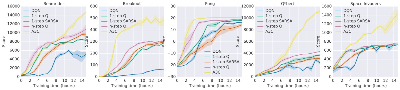
Figure 1: Learning speed comparison for DQN and the new asynchronous algorithms on five Atari 2600 games. DQN was trained on a single Nvidia K40 GPU while the asynchronous methods were trained using 16 CPU cores. The plots are averaged over 5 runs. In the case of DQN the runs were for different seeds with fixed hyperparameters. For asynchronous methods we average over the best 5 models from 50 experiments with learning rates sampled from and all other hyperparameters fixed.
图 1:DQN 与新异步算法在五个 Atari 2600 游戏上的学习速度比较。DQN 在单块 Nvidia K40 GPU 上训练,异步方法用 16 个 CPU 核训练。曲线对 5 次运行取平均。对 DQN,运行为固定超参下不同种子。对异步方法,我们从学习率按 采样、其余超参固定的 50 次实验中,对最好的 5 个模型取平均。
We use four different platforms for assessing the properties of the proposed framework. We perform most of our experiments using the Arcade Learning Environment (Bellemare et al. 2012), which provides a simulator for Atari 2600 games. This is one of the most commonly used benchmark environments for RL algorithms. We use the Atari domain to compare against state of the art results (Van Hasselt et al. 2015; Wang et al. 2015; Schaul et al. 2015; Nair et al. 2015; Mnih et al. 2015), as well as to carry out a detailed stability and scalability analysis of the proposed methods. We performed further comparisons using the TORCS 3D car racing simulator (Wymann et al. 2013). We also use two additional domains to evaluate only the A3C algorithm – Mujoco and Labyrinth. MuJoCo (Todorov 2015) is a physics simulator for evaluating agents on continuous motor control tasks with contact dynamics. Labyrinth is a new 3D environment where the agent must learn to find rewards in randomly generated mazes from a visual input. The precise details of our experimental setup can be found in Supplementary Section 8.
我们用四个不同平台评估所提框架的性质。多数实验在 Arcade Learning Environment(Bellemare et al. 2012)上进行,它提供 Atari 2600 游戏模拟器。这是 RL 算法最常用的基准环境之一。我们用 Atari 领域与当时最优结果比较(Van Hasselt et al. 2015;Wang et al. 2015;Schaul et al. 2015;Nair et al. 2015;Mnih et al. 2015),并对所提方法做详细稳定性与可扩展性分析。我们还用 TORCS 3D 赛车模拟器(Wymann et al. 2013)做进一步比较。另外两个仅用于评估 A3C 算法的领域是 Mujoco 与 Labyrinth。MuJoCo(Todorov 2015)是评估带接触动力学的连续电机控制任务上智能体的物理模拟器。Labyrinth 是新的 3D 环境,智能体必须仅从视觉输入学习在随机生成迷宫中寻找奖励。实验设定的精确细节见补充第 8 节。
5.1 Atari 2600 Games
5.1 Atari 2600 游戏
We first present results on a subset of Atari 2600 games to demonstrate the training speed of the new methods. Figure 1 compares the learning speed of the DQN algorithm trained on an Nvidia K40 GPU with the asynchronous methods trained using 16 CPU cores on five Atari 2600 games. The results show that all four asynchronous methods we presented can successfully train neural network controllers on the Atari domain. The asynchronous methods tend to learn faster than DQN, with significantly faster learning on some games, while training on only 16 CPU cores. Additionally, the results suggest that n-step methods learn faster than one-step methods on some games. Overall, the policy-based advantage actor-critic method significantly outperforms all three value-based methods.
我们首先在 Atari 2600 游戏子集上给出结果,以展示新方法的训练速度。图 1 比较了在 Nvidia K40 GPU 上训练的 DQN 与用 16 个 CPU 核训练的异步方法在五个 Atari 2600 游戏上的学习速度。结果表明,我们给出的四种异步方法都能在 Atari 领域成功训练神经网络控制器。异步方法往往比 DQN 学得更快,在某些游戏上显著更快,同时只在 16 个 CPU 核上训练。此外,结果表明 n-step 方法在某些游戏上比一步方法学得更快。总体而言,基于策略的优势 actor-critic 方法显著优于全部三种基于价值的方法。
We then evaluated asynchronous advantage actor-critic on 57 Atari games. In order to compare with the state of the art in Atari game playing, we largely followed the training and evaluation protocol of (Van Hasselt et al. 2015). Specifically, we tuned hyperparameters (learning rate and amount of gradient norm clipping) using a search on six Atari games (Beamrider, Breakout, Pong, Q*bert, Seaquest and Space Invaders) and then fixed all hyperparameters for all 57 games. We trained both a feedforward agent with the same architecture as (Mnih et al. 2015; Nair et al. 2015; Van Hasselt et al. 2015) as well as a recurrent agent with an additional 256 LSTM cells after the final hidden layer. We additionally used the final network weights for evaluation to make the results more comparable to the original results from (Bellemare et al. 2012). We trained our agents for four days using 16 CPU cores, while the other agents were trained for 8 to 10 days on Nvidia K40 GPUs. Table 1 shows the average and median human-normalized scores obtained by our agents trained by asynchronous advantage actor-critic (A3C) as well as the current state-of-the art. Supplementary Table S3 shows the scores on all games. A3C significantly improves on state-of-the-art the average score over 57 games in half the training time of the other methods while using only 16 CPU cores and no GPU. Furthermore, after just one day of training, A3C matches the average human normalized score of Dueling Double DQN and almost reaches the median human normalized score of Gorila. We note that many of the improvements that are presented in Double DQN (Van Hasselt et al. 2015) and Dueling Double DQN (Wang et al. 2015) can be incorporated to 1-step Q and n-step Q methods presented in this work with similar potential improvements.
我们随后在 57 个 Atari 游戏上评估异步优势 actor-critic。为与 Atari 游戏对弈的当时最优比较,我们大体遵循(Van Hasselt et al. 2015)的训练与评测协议。具体地,我们在六个 Atari 游戏(Beamrider、Breakout、Pong、Q*bert、Seaquest 与 Space Invaders)上搜索调超参(学习率与梯度范数裁剪量),然后对全部 57 个游戏固定所有超参。我们既训练与(Mnih et al. 2015;Nair et al. 2015;Van Hasselt et al. 2015)相同架构的前馈智能体,也训练在最终隐层后额外加 256 个 LSTM 单元的循环智能体。我们还用最终网络权重做评测,以使结果更可比于(Bellemare et al. 2012)的原始结果。我们用 16 个 CPU 核训练智能体四天,而其他智能体在 Nvidia K40 GPU 上训练 8 到 10 天。表 1 给出由异步优势 actor-critic(A3C)训练的智能体以及当时最优所获得的平均与中位人类归一化分数。补充表 S3 给出全部游戏上的分数。A3C 在其他方法一半训练时间内、仅用 16 个 CPU 核且无 GPU,显著改进了 57 个游戏上的平均分数最优水平。此外,仅训练一天后,A3C 就匹配 Dueling Double DQN 的平均人类归一化分数,并几乎达到 Gorila 的中位人类归一化分数。我们指出,Double DQN(Van Hasselt et al. 2015)与 Dueling Double DQN(Wang et al. 2015)中给出的许多改进,也可并入本文给出的 1-step Q 与 n-step Q 方法,并有类似潜在提升。
| Method | Training Time | Mean | Median |
|---|---|---|---|
| DQN | 8 days on GPU | 121.9% | 47.5% |
| Gorila | 4 days, 100 machines | 215.2% | 71.3% |
| D-DQN | 8 days on GPU | 332.9% | 110.9% |
| Dueling D-DQN | 8 days on GPU | 343.8% | 117.1% |
| Prioritized DQN | 8 days on GPU | 463.6% | 127.6% |
| A3C, FF | 1 day on CPU | 344.1% | 68.2% |
| A3C, FF | 4 days on CPU | 496.8% | 116.6% |
| A3C, LSTM | 4 days on CPU | 623.0% | 112.6% |
Table 1: Mean and median human-normalized scores on 57 Atari games using the human starts evaluation metric. Supplementary Table SS3 shows the raw scores for all games.
| Method | Training Time | Mean | Median |
|---|---|---|---|
| DQN | 8 days on GPU | 121.9% | 47.5% |
| Gorila | 4 days, 100 machines | 215.2% | 71.3% |
| D-DQN | 8 days on GPU | 332.9% | 110.9% |
| Dueling D-DQN | 8 days on GPU | 343.8% | 117.1% |
| Prioritized DQN | 8 days on GPU | 463.6% | 127.6% |
| A3C, FF | 1 day on CPU | 344.1% | 68.2% |
| A3C, FF | 4 days on CPU | 496.8% | 116.6% |
| A3C, LSTM | 4 days on CPU | 623.0% | 112.6% |
表 1:在 57 个 Atari 游戏上用 human starts 评测指标得到的平均与中位人类归一化分数。补充表 SS3 给出全部游戏的原始分数。
5.2 TORCS Car Racing Simulator
5.2 TORCS 赛车模拟器
We also compared the four asynchronous methods on the TORCS 3D car racing game (Wymann et al. 2013). TORCS not only has more realistic graphics than Atari 2600 games, but also requires the agent to learn the dynamics of the car it is controlling. At each step, an agent received only a visual input in the form of an RGB image of the current frame as well as a reward proportional to the agent’s velocity along the center of the track at the agent’s current position. We used the same neural network architecture as the one used in the Atari experiments specified in Supplementary Section 8. We performed experiments using four different settings – the agent controlling a slow car with and without opponent bots, and the agent controlling a fast car with and without opponent bots. Full results can be found in Supplementary Figure S6. A3C was the best performing agent, reaching between roughly and of the score obtained by a human tester on all four game configurations in about 12 hours of training. A video showing the learned driving behavior of the A3C agent can be found at https://youtu.be/0xo1Ldx3L5Q.
我们还在 TORCS 3D 赛车游戏(Wymann et al. 2013)上比较四种异步方法。TORCS 不仅比 Atari 2600 游戏有更真实的图形,还要求智能体学习其所控制汽车的动力学。在每一步,智能体仅收到当前帧 RGB 图像形式的视觉输入,以及与智能体当前位置沿赛道中心速度成比例的奖励。我们使用与 Atari 实验相同的神经网络架构,见补充第 8 节。我们在四种不同设定下做实验——智能体控制慢车有无对手机器人,以及控制快车有无对手机器人。完整结果见补充图 S6。A3C 是表现最好的智能体,在约 12 小时训练内,在全部四种游戏配置上达到人类测试者所得分数的大约 到 。展示 A3C 智能体所学驾驶行为的视频见 https://youtu.be/0xo1Ldx3L5Q。
5.3 Continuous Action Control Using the MuJoCo Physics Simulator
5.3 用 MuJoCo 物理模拟器做连续动作控制
We also examined a set of tasks where the action space is continuous. In particular, we looked at a set of rigid body physics domains with contact dynamics where the tasks include many examples of manipulation and locomotion. These tasks were simulated using the Mujoco physics engine. We evaluated only the asynchronous advantage actor-critic algorithm since, unlike the value-based methods, it is easily extended to continuous actions. In all problems, using either the physical state or pixels as input, Asynchronous Advantage-Critic found good solutions in less than 24 hours of training and typically in under a few hours. Some successful policies learned by our agent can be seen in the following video https://youtu.be/Ajjc08-iPx8. Further details about this experiment can be found in Supplementary Section 9.
我们还考察了一组动作空间连续的任务。具体地,我们看一组带接触动力学的刚体物理领域,任务包括许多操作与运动例子。这些任务用 Mujoco 物理引擎模拟。我们只评估异步优势 actor-critic 算法,因为与基于价值的方法不同,它易于扩展到连续动作。在所有问题上,无论用物理状态还是像素作输入,异步优势 Critic 都在不到 24 小时训练内找到好解,通常只需数小时。智能体学到的一些成功策略见视频 https://youtu.be/Ajjc08-iPx8。该实验的进一步细节见补充第 9 节。
5.4 Labyrinth
We performed an additional set of experiments with A3C on a new 3D environment called Labyrinth. The specific task we considered involved the agent learning to find rewards in randomly generated mazes. At the beginning of each episode the agent was placed in a new randomly generated maze consisting of rooms and corridors. Each maze contained two types of objects that the agent was rewarded for finding – apples and portals. Picking up an apple led to a reward of . Entering a portal led to a reward of after which the agent was respawned in a new random location in the maze and all previously collected apples were regenerated. An episode terminated after 60 seconds after which a new episode would begin. The aim of the agent is to collect as many points as possible in the time limit and the optimal strategy involves first finding the portal and then repeatedly going back to it after each respawn. This task is much more challenging than the TORCS driving domain because the agent is faced with a new maze in each episode and must learn a general strategy for exploring random mazes.
我们在称为 Labyrinth 的新 3D 环境上用 A3C 做了额外一组实验。所考虑的具体任务是智能体学习在随机生成迷宫中寻找奖励。每个回合开始时,智能体被置于由房间与走廊组成的新随机迷宫中。每个迷宫含两类智能体找到即可获奖励的物体——苹果与传送门。捡起苹果得到奖励 。进入传送门得到奖励 ,之后智能体在迷宫中新的随机位置重生,且所有先前收集的苹果重新生成。回合在 60 秒后终止,随后开始新回合。智能体目标是在时限内尽可能多得分,最优策略是先找到传送门,再在每次重生后反复回到它。该任务比 TORCS 驾驶领域更具挑战,因为智能体每个回合面对新迷宫,必须学习探索随机迷宫的一般策略。
We trained an A3C LSTM agent on this task using only RGB images as input. The final average score of around 50 indicates that the agent learned a reasonable strategy for exploring random 3D maxes using only a visual input. A video showing one of the agents exploring previously unseen mazes is included at https://youtu.be/nMR5mjCFZCw.
我们在该任务上仅用 RGB 图像作输入训练 A3C LSTM 智能体。最终平均分数约 50,表明智能体学到了仅用视觉输入探索随机 3D 迷宫的合理策略。展示其中一个智能体探索先前未见迷宫的视频见 https://youtu.be/nMR5mjCFZCw。
5.5 Scalability and Data Efficiency
5.5 可扩展性与数据效率
| Number of threads | |||||
|---|---|---|---|---|---|
| Method | 1 | 2 | 4 | 8 | 16 |
| 1-step Q | 1.0 | 3.0 | 6.3 | 13.3 | 24.1 |
| 1-step SARSA | 1.0 | 2.8 | 5.9 | 13.1 | 22.1 |
| n-step Q | 1.0 | 2.7 | 5.9 | 10.7 | 17.2 |
| A3C | 1.0 | 2.1 | 3.7 | 6.9 | 12.5 |
Table 2: The average training speedup for each method and number of threads averaged over seven Atari games. To compute the training speed-up on a single game we measured the time to required reach a fixed reference score using each method and number of threads. The speedup from using threads on a game was defined as the time required to reach a fixed reference score using one thread divided the time required to reach the reference score using threads. The table shows the speedups averaged over seven Atari games (Beamrider, Breakout, Enduro, Pong, Q*bert, Seaquest, and Space Invaders).
| Number of threads | |||||
|---|---|---|---|---|---|
| Method | 1 | 2 | 4 | 8 | 16 |
| 1-step Q | 1.0 | 3.0 | 6.3 | 13.3 | 24.1 |
| 1-step SARSA | 1.0 | 2.8 | 5.9 | 13.1 | 22.1 |
| n-step Q | 1.0 | 2.7 | 5.9 | 10.7 | 17.2 |
| A3C | 1.0 | 2.1 | 3.7 | 6.9 | 12.5 |
表 2:七个 Atari 游戏上各方法与线程数的平均训练加速。为计算单游戏训练加速,我们测量各方法与线程数达到固定参考分数所需时间。某游戏上用 线程的加速定义为用一线程达到固定参考分数所需时间除以用 线程达到参考分数所需时间。表中给出七个 Atari 游戏(Beamrider、Breakout、Enduro、Pong、Q*bert、Seaquest 与 Space Invaders)上的平均加速。

Figure 2: Scatter plots of scores obtained by asynchronous advantage actor-critic on five games (Beamrider, Breakout, Pong, Q*bert, Space Invaders) for different learning rates and random initializations. On each game, there is a wide range of learning rates for which all random initializations acheive good scores. This shows that A3C is quite robust to learning rates and initial random weights.
图 2:异步优势 actor-critic 在五个游戏(Beamrider、Breakout、Pong、Q*bert、Space Invaders)上、对 种不同学习率与随机初始化所得分数的散点图。在每个游戏上,都有很宽的学习率范围使所有随机初始化都取得好分数。这表明 A3C 对学习率与初始随机权重相当稳健。
We analyzed the effectiveness of our proposed framework by looking at how the training time and data efficiency changes with the number of parallel actor-learners. When using multiple workers in parallel and updating a shared model, one would expect that in an ideal case, for a given task and algorithm, the number of training steps to achieve a certain score would remain the same with varying numbers of workers. Therefore, the advantage would be solely due to the ability of the system to consume more data in the same amount of wall clock time and possibly improved exploration. Table 2 shows the training speed-up achieved by using increasing numbers of parallel actor-learners averaged over seven Atari games. These results show that all four methods achieve substantial speedups from using multiple worker threads, with threads leading to at least an order of magnitude speedup. This confirms that our proposed framework scales well with the number of parallel workers, making efficient use of resources.
我们通过分析训练时间与数据效率如何随并行 actor-learner 数量变化,来分析所提框架的有效性。当并行使用多个 worker 并更新共享模型时,理想情况下,对给定任务与算法,达到某一分数所需训练步数应随 worker 数量变化保持不变。因此优势将仅来自系统在相同墙钟时间内消耗更多数据的能力,以及可能改善的探索。表 2 给出在七个 Atari 游戏平均下、使用递增数量并行 actor-learner 所达到的训练加速。这些结果表明四种方法都从使用多个 worker 线程获得显著加速, 线程至少带来一个数量级加速。这证实所提框架随并行 worker 数量良好扩展,能高效利用资源。
Somewhat surprisingly, asynchronous one-step Q-learning and Sarsa algorithms exhibit superlinear speedups that cannot be explained by purely computational gains. We observe that one-step methods (one-step Q and one-step Sarsa) often require less data to achieve a particular score when using more parallel actor-learners. We believe this is due to positive effect of multiple threads to reduce the bias in one-step methods. These effects are shown more clearly in Figure 3, which shows plots of the average score against the total number of training frames for different numbers of actor-learners and training methods on five Atari games, and Figure 4, which shows plots of the average score against wall-clock time.
有些出人意料的是,异步一步 Q-learning 与 Sarsa 算法表现出超线性加速,无法仅用计算收益解释。我们观察到:一步方法(一步 Q 与一步 Sarsa)在使用更多并行 actor-learner 时,达到特定分数往往需要更少数据。我们相信这是由于多线程对降低一步方法偏置的积极作用。这些效应在图 3 中更清楚:该图给出五个 Atari 游戏上不同 actor-learner 数量与训练方法下平均分数相对总训练帧数的曲线;图 4 给出平均分数相对墙钟时间的曲线。
5.6 Robustness and Stability
5.6 稳健性与稳定性
Finally, we analyzed the stability and robustness of the four proposed asynchronous algorithms. For each of the four algorithms we trained models on five games (Breakout, Beamrider, Pong, Q*bert, Space Invaders) using different learning rates and random initializations. Figure 2 shows scatter plots of the resulting scores for A3C, while Supplementary Figure S11 shows plots for the other three methods. There is usually a range of learning rates for each method and game combination that leads to good scores, indicating that all methods are quite robust to the choice of learning rate and random initialization. The fact that there are virtually no points with scores of in regions with good learning rates indicates that the methods are stable and do not collapse or diverge once they are learning.
最后,我们分析四种所提异步算法的稳定性与稳健性。对四种算法中的每一种,我们在五个游戏(Breakout、Beamrider、Pong、Q*bert、Space Invaders)上用 种不同学习率与随机初始化训练模型。图 2 给出 A3C 所得分数的散点图,补充图 S11 给出另外三种方法的图。通常对每种方法与游戏组合都有一段学习率范围导致好分数,表明所有方法对学习率选择与随机初始化都相当稳健。在具有良好学习率的区域几乎没有分数为 的点,表明方法稳定,一旦开始学习就不会崩溃或发散。

Figure 3: Data efficiency comparison of different numbers of actor-learners for three asynchronous methods on five Atari games. The x-axis shows the total number of training epochs where an epoch corresponds to four million frames (across all threads). The y-axis shows the average score. Each curve shows the average over the three best learning rates. Single step methods show increased data efficiency from more parallel workers. Results for Sarsa are shown in Supplementary Figure S9.
图 3:三个异步方法在五个 Atari 游戏上不同 actor-learner 数量的数据效率比较。横轴为总训练 epoch 数,一个 epoch 对应四百万帧(跨所有线程)。纵轴为平均分数。每条曲线对三个最佳学习率取平均。一步方法因更多并行 worker 而显示更高数据效率。Sarsa 结果见补充图 S9。

Figure 4: Training speed comparison of different numbers of actor-learners on five Atari games. The x-axis shows training time in hours while the y-axis shows the average score. Each curve shows the average over the three best learning rates. All asynchronous methods show significant speedups from using greater numbers of parallel actor-learners. Results for Sarsa are shown in Supplementary Figure S10.
图 4:五个 Atari 游戏上不同 actor-learner 数量的训练速度比较。横轴为训练时间(小时),纵轴为平均分数。每条曲线对三个最佳学习率取平均。所有异步方法都因使用更多并行 actor-learner 而显示显著加速。Sarsa 结果见补充图 S10。
6 Conclusions and Discussion
6 结论与讨论
We have presented asynchronous versions of four standard reinforcement learning algorithms and showed that they are able to train neural network controllers on a variety of domains in a stable manner. Our results show that in our proposed framework stable training of neural networks through reinforcement learning is possible with both value-based and policy-based methods, off-policy as well as on-policy methods, and in discrete as well as continuous domains. When trained on the Atari domain using 16 CPU cores, the proposed asynchronous algorithms train faster than DQN trained on an Nvidia K40 GPU, with A3C surpassing the current state-of-the-art in half the training time.
我们给出了四种标准强化学习算法的异步版本,并表明它们能在多种领域上以稳定方式训练神经网络控制器。结果表明:在我们提出的框架中,通过强化学习稳定训练神经网络,对基于价值与基于策略的方法、离策略与在策略方法、离散与连续领域都是可能的。用 16 个 CPU 核在 Atari 领域训练时,所提异步算法比在 Nvidia K40 GPU 上训练的 DQN 更快,且 A3C 以一半训练时间超过当时最优。
One of our main findings is that using parallel actor-learners to update a shared model had a stabilizing effect on the learning process of the three value-based methods we considered. While this shows that stable online Q-learning is possible without experience replay, which was used for this purpose in DQN, it does not mean that experience replay is not useful. Incorporating experience replay into the asynchronous reinforcement learning framework could substantially improve the data efficiency of these methods by reusing old data. This could in turn lead to much faster training times in domains like TORCS where interacting with the environment is more expensive than updating the model for the architecture we used.
我们的主要发现之一是:用并行 actor-learner 更新共享模型,对我们考虑的三种基于价值方法的学习过程有稳定作用。这虽表明无经验回放的稳定在线 Q-learning 是可能的(DQN 为此使用经验回放),但并不意味着经验回放无用。把经验回放并入异步强化学习框架,可通过重用旧数据显著改善这些方法的数据效率。这进而可在 TORCS 等与环境交互比我们所用架构更新模型更昂贵的领域带来快得多的训练时间。
Combining other existing reinforcement learning methods or recent advances in deep reinforcement learning with our asynchronous framework presents many possibilities for immediate improvements to the methods we presented. While our n-step methods operate in the forward view (Sutton & Barto 1998) by using corrected n-step returns directly as targets, it has been more common to use the backward view to implicitly combine different returns through eligibility traces (Watkins 1989; Sutton & Barto 1998; Peng & Williams 1996). The asynchronous advantage actor-critic method could be potentially improved by using other ways of estimating the advantage function, such as generalized advantage estimation of (Schulman et al. 2015b). All of the value-based methods we investigated could benefit from different ways of reducing over-estimation bias of Q-values (Van Hasselt et al. 2015; Bellemare et al. 2016). Yet another, more speculative, direction is to try and combine the recent work on true online temporal difference methods (van Seijen et al. 2015) with nonlinear function approximation.
把其他现有强化学习方法或深度强化学习近期进展与我们的异步框架结合,为立即改进我们所提方法提供许多可能。我们的 n-step 方法通过直接用校正后的 n-step 回报作目标以前向视角(Sutton & Barto 1998)运行,而更常见的是用后向视角通过资格迹隐式组合不同回报(Watkins 1989;Sutton & Barto 1998;Peng & Williams 1996)。异步优势 actor-critic 方法潜在地可通过其他估计优势函数的方式改进,例如(Schulman et al. 2015b)的广义优势估计。我们考察的全部基于价值方法都可受益于降低 Q 值过高估计偏置的不同方式(Van Hasselt et al. 2015;Bellemare et al. 2016)。另一更带推测性的方向,是尝试把真正在线时序差分方法的近期工作(van Seijen et al. 2015)与非线性函数逼近结合。
In addition to these algorithmic improvements, a number of complementary improvements to the neural network architecture are possible. The dueling architecture of (Wang et al. 2015) has been shown to produce more accurate estimates of Q-values by including separate streams for the state value and advantage in the network. The spatial softmax proposed by (Levine et al. 2015) could improve both value-based and policy-based methods by making it easier for the network to represent feature coordinates.
除这些算法改进外,对神经网络架构也可能有若干互补改进。(Wang et al. 2015)的对决架构通过在网络中包含状态价值与优势的分离流,已被表明产生更准确的 Q 值估计。(Levine et al. 2015)提出的空间 softmax 可通过使网络更容易表示特征坐标,改进基于价值与基于策略的方法。
Acknowledgments
We thank Thomas Degris, Remi Munos, Marc Lanctot, Sasha Vezhnevets and Joseph Modayil for many helpful discussions, suggestions and comments on the paper. We also thank the DeepMind evaluation team for setting up the environments used to evaluate the agents in the paper.
致谢
我们感谢 Thomas Degris、Remi Munos、Marc Lanctot、Sasha Vezhnevets 与 Joseph Modayil 的许多有益讨论、建议与对论文的评论。我们也感谢 DeepMind 评测团队搭建用于评估文中智能体的环境。
References
参考文献
Bellemare et al. (2012) Bellemare, Marc G, Naddaf, Yavar, Veness, Joel, and Bowling, Michael. The arcade learning environment: An evaluation platform for general agents. Journal of Artificial Intelligence Research , 2012.
Bellemare et al. (2016) Bellemare, Marc G., Ostrovski, Georg, Guez, Arthur, Thomas, Philip S., and Munos, Rémi. Increasing the action gap: New operators for reinforcement learning. In Proceedings of the AAAI Conference on Artificial Intelligence , 2016.
Bertsekas (1982) Bertsekas, Dimitri P. Distributed dynamic programming. Automatic Control, IEEE Transactions on , 27(3):610–616, 1982.
Chavez et al. (2015) Chavez, Kevin, Ong, Hao Yi, and Hong, Augustus. Distributed deep q-learning. Technical report, Stanford University, June 2015.
Degris et al. (2012) Degris, Thomas, Pilarski, Patrick M, and Sutton, Richard S. Model-free reinforcement learning with continuous action in practice. In American Control Conference (ACC), 2012 , pp. 2177–2182. IEEE, 2012.
Grounds & Kudenko (2008) Grounds, Matthew and Kudenko, Daniel. Parallel reinforcement learning with linear function approximation. In Proceedings of the 5th, 6th and 7th European Conference on Adaptive and Learning Agents and Multi-agent Systems: Adaptation and Multi-agent Learning , pp. 60–74. Springer-Verlag, 2008.
Koutník et al. (2014) Koutník, Jan, Schmidhuber, Jürgen, and Gomez, Faustino. Evolving deep unsupervised convolutional networks for vision-based reinforcement learning. In Proceedings of the 2014 conference on Genetic and evolutionary computation , pp. 541–548. ACM, 2014.
Levine et al. (2015) Levine, Sergey, Finn, Chelsea, Darrell, Trevor, and Abbeel, Pieter. End-to-end training of deep visuomotor policies. arXiv preprint arXiv:1504.00702 , 2015.
Li & Schuurmans (2011) Li, Yuxi and Schuurmans, Dale. Mapreduce for parallel reinforcement learning. In Recent Advances in Reinforcement Learning - 9th European Workshop, EWRL 2011, Athens, Greece, September 9-11, 2011, Revised Selected Papers , pp. 309–320, 2011.
Lillicrap et al. (2015) Lillicrap, Timothy P, Hunt, Jonathan J, Pritzel, Alexander, Heess, Nicolas, Erez, Tom, Tassa, Yuval, Silver, David, and Wierstra, Daan. Continuous control with deep reinforcement learning. arXiv preprint arXiv:1509.02971 , 2015.
Mnih et al. (2013) Mnih, Volodymyr, Kavukcuoglu, Koray, Silver, David, Graves, Alex, Antonoglou, Ioannis, Wierstra, Daan, and Riedmiller, Martin. Playing atari with deep reinforcement learning. In NIPS Deep Learning Workshop . 2013.
Mnih et al. (2015) Mnih, Volodymyr, Kavukcuoglu, Koray, Silver, David, Rusu, Andrei A., Veness, Joel, Bellemare, Marc G., Graves, Alex, Riedmiller, Martin, Fidjeland, Andreas K., Ostrovski, Georg, Petersen, Stig, Beattie, Charles, Sadik, Amir, Antonoglou, Ioannis, King, Helen, Kumaran, Dharshan, Wierstra, Daan, Legg, Shane, and Hassabis, Demis. Human-level control through deep reinforcement learning. Nature , 518(7540):529–533, 02 2015. URL http://dx.doi.org/10.1038/nature14236 .
Nair et al. (2015) Nair, Arun, Srinivasan, Praveen, Blackwell, Sam, Alcicek, Cagdas, Fearon, Rory, Maria, Alessandro De, Panneershelvam, Vedavyas, Suleyman, Mustafa, Beattie, Charles, Petersen, Stig, Legg, Shane, Mnih, Volodymyr, Kavukcuoglu, Koray, and Silver, David. Massively parallel methods for deep reinforcement learning. In ICML Deep Learning Workshop . 2015.
Peng & Williams (1996) Peng, Jing and Williams, Ronald J. Incremental multi-step q-learning. Machine Learning , 22(1-3):283–290, 1996.
Recht et al. (2011) Recht, Benjamin, Re, Christopher, Wright, Stephen, and Niu, Feng. Hogwild: A lock-free approach to parallelizing stochastic gradient descent. In Advances in Neural Information Processing Systems , pp. 693–701, 2011.
Riedmiller (2005) Riedmiller, Martin. Neural fitted q iteration–first experiences with a data efficient neural reinforcement learning method. In Machine Learning: ECML 2005 , pp. 317–328. Springer Berlin Heidelberg, 2005.
Rummery & Niranjan (1994) Rummery, Gavin A and Niranjan, Mahesan. On-line q-learning using connectionist systems. 1994.
Schaul et al. (2015) Schaul, Tom, Quan, John, Antonoglou, Ioannis, and Silver, David. Prioritized experience replay. arXiv preprint arXiv:1511.05952 , 2015.
Schulman et al. (2015a) Schulman, John, Levine, Sergey, Moritz, Philipp, Jordan, Michael I, and Abbeel, Pieter. Trust region policy optimization. In International Conference on Machine Learning (ICML) , 2015a.
Schulman et al. (2015b) Schulman, John, Moritz, Philipp, Levine, Sergey, Jordan, Michael, and Abbeel, Pieter. High-dimensional continuous control using generalized advantage estimation. arXiv preprint arXiv:1506.02438 , 2015b.
Sutton & Barto (1998) Sutton, R. and Barto, A. Reinforcement Learning: an Introduction . MIT Press, 1998.
Tieleman & Hinton (2012) Tieleman, Tijmen and Hinton, Geoffrey. Lecture 6.5-rmsprop: Divide the gradient by a running average of its recent magnitude. COURSERA: Neural Networks for Machine Learning , 4, 2012.
Todorov (2015) Todorov, E. MuJoCo: Modeling, Simulation and Visualization of Multi-Joint Dynamics with Contact (ed 1.0) . Roboti Publishing, 2015.
Tomassini (1999) Tomassini, Marco. Parallel and distributed evolutionary algorithms: A review. Technical report, 1999.
Tsitsiklis (1994) Tsitsiklis, John N. Asynchronous stochastic approximation and q-learning. Machine Learning , 16(3):185–202, 1994.
Van Hasselt et al. (2015) Van Hasselt, Hado, Guez, Arthur, and Silver, David. Deep reinforcement learning with double q-learning. arXiv preprint arXiv:1509.06461 , 2015.
van Seijen et al. (2015) van Seijen, H., Rupam Mahmood, A., Pilarski, P. M., Machado, M. C., and Sutton, R. S. True Online Temporal-Difference Learning. ArXiv e-prints , December 2015.
Wang et al. (2015) Wang, Z., de Freitas, N., and Lanctot, M. Dueling Network Architectures for Deep Reinforcement Learning. ArXiv e-prints , November 2015.
Watkins (1989) Watkins, Christopher John Cornish Hellaby. Learning from delayed rewards . PhD thesis, University of Cambridge England, 1989.
Williams (1992) Williams, R.J. Simple statistical gradient-following algorithms for connectionist reinforcement learning. Machine Learning , 8(3):229–256, 1992.
Williams & Peng (1991) Williams, Ronald J and Peng, Jing. Function optimization using connectionist reinforcement learning algorithms. Connection Science , 3(3):241–268, 1991.
Wymann et al. (2013) Wymann, B., Espié, E., Guionneau, C., Dimitrakakis, C., Coulom, R., and Sumner, A. Torcs: The open racing car simulator, v1.3.5, 2013.
7 Optimization Details
7 优化细节
We investigated two different optimization algorithms with our asynchronous framework – stochastic gradient descent and RMSProp. Our implementations of these algorithms do not use any locking in order to maximize throughput when using a large number of threads.
我们在异步框架中考察了两种不同优化算法——随机梯度下降与 RMSProp。这些算法的实现对锁不做任何使用,以便在使用大量线程时最大化吞吐。
Momentum SGD: The implementation of SGD in an asynchronous setting is relatively straightforward and well studied (Recht et al. 2011). Let be the parameter vector that is shared across all threads and let be the accumulated gradients of the loss with respect to parameters computed by thread number . Each thread independently applies the standard momentum SGD update followed by with learning rate , momentum and without any locks. Note that in this setting, each thread maintains its own separate gradient and momentum vector.
动量 SGD: 异步设定下 SGD 的实现相对直接且研究充分(Recht et al. 2011)。设 为跨所有线程共享的参数向量, 为线程 计算的损失相对参数 的累积梯度。每个线程 独立应用标准动量 SGD 更新 ,随后 ,学习率为 、动量为 ,且不加锁。注意在此设定下,每个线程维护自己单独的梯度与动量向量。
RMSProp: While RMSProp (Tieleman & Hinton 2012) has been widely used in the deep learning literature, it has not been extensively studied in the asynchronous optimization setting. The standard non-centered RMSProp update is given by
RMSProp: 尽管 RMSProp(Tieleman & Hinton 2012)在深度学习文献中被广泛使用,在异步优化设定下尚未被充分研究。标准非中心化 RMSProp 更新为
where all operations are performed elementwise. In order to apply RMSProp in the asynchronous optimization setting one must decide whether the moving average of elementwise squared gradients is shared or per-thread. We experimented with two versions of the algorithm. In one version, which we refer to as RMSProp, each thread maintains its own shown in Equation S2. In the other version, which we call Shared RMSProp, the vector is shared among threads and is updated asynchronously and without locking. Sharing statistics among threads also reduces memory requirements by using one fewer copy of the parameter vector per thread.
其中所有运算按元素进行。为在异步优化设定中应用 RMSProp,必须决定逐元素平方梯度的滑动平均 是共享还是每线程一份。我们实验了算法的两个版本。在一个称为 RMSProp 的版本中,每个线程维护自己的式 S2 中的 。在另一个称为 Shared RMSProp 的版本中,向量 在线程间共享,并异步、无锁更新。在线程间共享统计量也通过每线程少用一份参数向量副本降低内存需求。
We compared these three asynchronous optimization algorithms in terms of their sensitivity to different learning rates and random network initializations. Figure S5 shows a comparison of the methods for two different reinforcement learning methods (Async -step Q and Async Advantage Actor-Critic) on four different games (Breakout, Beamrider, Seaquest and Space Invaders). Each curve shows the scores for 50 experiments that correspond to 50 different random learning rates and initializations. The x-axis shows the rank of the model after sorting in descending order by final average score and the y-axis shows the final average score achieved by the corresponding model. In this representation, the algorithm that performs better would achieve higher maximum rewards on the y-axis and the algorithm that is most robust would have its slope closest to horizontal, thus maximizing the area under the curve. RMSProp with shared statistics tends to be more robust than RMSProp with per-thread statistics, which is in turn more robust than Momentum SGD.
我们比较这三种异步优化算法对不同学习率与随机网络初始化的敏感性。图 S5 给出两种不同强化学习方法(异步 -step Q 与异步优势 Actor-Critic)在四个不同游戏(Breakout、Beamrider、Seaquest 与 Space Invaders)上的方法比较。每条曲线给出对应 50 种不同随机学习率与初始化的 50 次实验分数。横轴为按最终平均分数降序排序后的模型排名,纵轴为对应模型达到的最终平均分数。在此表示下,表现更好的算法会在纵轴上达到更高最大奖励,最稳健的算法斜率最接近水平,从而最大化曲线下面积。带共享统计量的 RMSProp 往往比每线程统计量的 RMSProp 更稳健,后者又比动量 SGD 更稳健。
8 Experimental Setup
8 实验设定
The experiments performed on a subset of Atari games (Figures 1, 3, 4 and Table 2) as well as the TORCS experiments (Figure S6) used the following setup. Each experiment used 16 actor-learner threads running on a single machine and no GPUs. All methods performed updates after every 5 actions ( and ) and shared RMSProp was used for optimization. The three asynchronous value-based methods used a shared target network that was updated every 40000 frames. The Atari experiments used the same input preprocessing as (Mnih et al. 2015) and an action repeat of 4. The agents used the network architecture from (Mnih et al. 2013). The network used a convolutional layer with 16 filters of size with stride 4, followed by a convolutional layer with with 32 filters of size with stride 2, followed by a fully connected layer with 256 hidden units. All three hidden layers were followed by a rectifier nonlinearity. The value-based methods had a single linear output unit for each action representing the action-value. The model used by actor-critic agents had two set of outputs – a softmax output with one entry per action representing the probability of selecting the action, and a single linear output representing the value function. All experiments used a discount of and an RMSProp decay factor of .
在 Atari 游戏子集上做的实验(图 1、3、4 与表 2)以及 TORCS 实验(图 S6)使用如下设定。每次实验使用在单机上运行的 16 个 actor-learner 线程,无 GPU。所有方法每 5 个动作后执行更新( 且 ),并用共享 RMSProp 优化。三种异步基于价值方法使用每 40000 帧更新一次的共享目标网络。Atari 实验使用与(Mnih et al. 2015)相同的输入预处理,动作重复为 4。智能体使用(Mnih et al. 2013)的网络架构。网络使用 16 个大小 、步长 4 的滤波器的卷积层,随后是 32 个大小 、步长 2 的滤波器的卷积层,再是 256 隐单元的全连接层。三个隐层后都跟整流非线性。基于价值方法对每个动作有一个表示动作价值的线性输出单元。actor-critic 智能体使用的模型有两组输出——对每个动作一个条目的 softmax 输出表示选择该动作的概率,以及表示价值函数的单个线性输出。所有实验使用折扣 与 RMSProp 衰减因子 。
The value based methods sampled the exploration rate from a distribution taking three values with probabilities . The values of were annealed from to respectively over the first four million frames. Advantage actor-critic used entropy regularization with a weight for all Atari and TORCS experiments. We performed a set of experiments for five Atari games and every TORCS level, each using a different random initialization and initial learning rate. The initial learning rate was sampled from a distribution and annealed to over the course of training. Note that in comparisons to prior work (Tables 1 and S3) we followed standard evaluation protocol and used fixed hyperparameters.
基于价值方法从取三个值 、概率分别为 的分布中采样探索率 。 的值在前四百万帧内分别从 退火到 。优势 actor-critic 对全部 Atari 与 TORCS 实验使用权重 的熵正则。我们对五个 Atari 游戏与每个 TORCS 关卡做一组 次实验,每次使用不同随机初始化与初始学习率。初始学习率从 分布采样,并在训练过程中退火到 。注意在与先前工作比较时(表 1 与 S3)我们遵循标准评测协议并使用固定超参。
9 Continuous Action Control Using the MuJoCo Physics Simulator
9 用 MuJoCo 物理模拟器做连续动作控制
To apply the asynchronous advantage actor-critic algorithm to the Mujoco tasks the necessary setup is nearly identical to that used in the discrete action domains, so here we enumerate only the differences required for the continuous action domains. The essential elements for many of the tasks (i.e. the physics models and task objectives) are near identical to the tasks examined in (Lillicrap et al. 2015). However, the rewards and thus performance are not comparable for most of the tasks due to changes made by the developers of Mujoco which altered the contact model.
把异步优势 actor-critic 算法应用到 Mujoco 任务时,必要设定与离散动作领域几乎相同,因此这里只枚举连续动作领域所需差异。许多任务的基本要素(即物理模型与任务目标)与(Lillicrap et al. 2015)考察的任务近乎相同。但由于 Mujoco 开发者改动接触模型所带来的变化,多数任务的奖励从而表现并不可比。
For all the domains we attempted to learn the task using the physical state as input. The physical state consisted of the joint positions and velocities as well as the target position if the task required a target. In addition, for three of the tasks (pendulum, pointmass2D, and gripper) we also examined training directly from RGB pixel inputs. In the low dimensional physical state case, the inputs are mapped to a hidden state using one hidden layer with 200 ReLU units. In the cases where we used pixels, the input was passed through two layers of spatial convolutions without any non-linearity or pooling. In either case, the output of the encoder layers were fed to a single layer of 128 LSTM cells. The most important difference in the architecture is in the the output layer of the policy network. Unlike the discrete action domain where the action output is a Softmax, here the two outputs of the policy network are two real number vectors which we treat as the mean vector and scalar variance of a multidimensional normal distribution with a spherical covariance. To act, the input is passed through the model to the output layer where we sample from the normal distribution determined by and . In practice, is modeled by a linear layer and by a SoftPlus operation, , as the activation computed as a function of the output of a linear layer. In our experiments with continuous control problems the networks for policy network and value network do not share any parameters, though this detail is unlikely to be crucial. Finally, since the episodes were typically at most several hundred time steps long, we did not use any bootstrapping in the policy or value function updates and batched each episode into a single update.
对所有领域,我们尝试用物理状态作输入学习任务。物理状态由关节位置与速度组成,若任务需要目标则还包括目标位置。此外,对三个任务(pendulum、pointmass2D 与 gripper),我们也考察直接从 RGB 像素输入训练。在低维物理状态情形,输入用一层 200 个 ReLU 单元的隐层映射到隐状态。在使用像素的情形,输入经过两层空间卷积,无非线性也无池化。无论哪种情形,编码器层输出都送入一层 128 个 LSTM 单元。架构最重要的差异在策略网络的输出层。与动作输出为 Softmax 的离散动作领域不同,此处策略网络的两个输出是两个实数向量,我们将其视为具有球面协方差的多维正态分布的均值向量 与标量方差 。行动时,输入穿过模型到达输出层,我们从由 与 确定的正态分布采样。实践中, 由线性层建模, 由 SoftPlus 运算 作为线性层输出函数的激活来建模。在连续控制问题实验中,策略网络与价值网络不共享任何参数,不过这一细节不太可能至关重要。最后,由于回合通常最多数百时间步长,我们在策略或价值函数更新中不使用任何自举,并把每个回合批成单次更新。
As in the discrete action case, we included an entropy cost which encouraged exploration. In the continuous case the we used a cost on the differential entropy of the normal distribution defined by the output of the actor network, , we used a constant multiplier of for this cost across all of the tasks examined. The asynchronous advantage actor-critic algorithm finds solutions for all the domains. Figure S8 shows learning curves against wall-clock time, and demonstrates that most of the domains from states can be solved within a few hours. All of the experiments, including those done from pixel based observations, were run on CPU. Even in the case of solving the domains directly from pixel inputs we found that it was possible to reliably discover solutions within 24 hours. Figure S7 shows scatter plots of the top scores against the sampled learning rates. In most of the domains there is large range of learning rates that consistently achieve good performance on the task.
与离散动作情形一样,我们加入鼓励探索的熵代价。在连续情形,我们对由 actor 网络输出定义的正态分布的微分熵使用代价 ,对所考察全部任务使用常数乘子 。异步优势 actor-critic 算法为所有领域找到解。图 S8 给出相对墙钟时间的学习曲线,并表明多数从状态出发的领域可在数小时内求解。所有实验——包括从基于像素观测做的实验——都在 CPU 上运行。即便在直接从像素输入求解领域的情形,我们也发现可在 24 小时内可靠发现解。图 S7 给出最高分相对采样学习率的散点图。在多数领域,有很宽的学习率范围能在任务上持续取得好表现。
// Assume global shared parameter vector .
// Assume global shared target parameter vector .
// Assume global shared counter .
Initialize thread step counter
Initialize target network parameters
Initialize thread-specific parameters
Initialize network gradients
repeat
Clear gradients
Synchronize thread-specific parameters
Get state
repeat
Take action according to the -greedy policy based on
Receive reward and new state
until terminal or
R=\left\{\begin{array}[]{l l}0&\text{for terminal }s_{t}\\ \max_{a}Q(s_{t},a;\theta^{-})&\text{for non-terminal }s_{t}\end{array}\right.
for do
Accumulate gradients wrt :
end for
Perform asynchronous update of using .
if then
end if
until
Algorithm S2 Asynchronous n-step Q-learning - pseudocode for each actor-learner thread.
// 假设全局共享 parameter vector .
// 假设全局共享 target parameter vector .
// 假设全局共享 counter .
Initialize thread step counter
Initialize target network parameters
Initialize thread-specific parameters
Initialize network gradients
repeat
Clear gradients
Synchronize thread-specific parameters
Get state
repeat
Take action according to the -greedy policy based on
Receive reward and new state
until terminal or
R=\left\{\begin{array}[]{l l}0&\text{for terminal }s_{t}\\ \max_{a}Q(s_{t},a;\theta^{-})&\text{for non-terminal }s_{t}\end{array}\right.
for do
Accumulate gradients wrt :
end for
Perform asynchronous update of using .
if then
end if
until
算法 S2 异步 n-step Q-learning——每个 actor-learner 线程的伪代码。
// Assume global shared parameter vectors and and global shared counter
// Assume thread-specific parameter vectors and
Initialize thread step counter
repeat
Reset gradients: and .
Synchronize thread-specific parameters and
Get state
repeat
Perform according to policy
Receive reward and new state
until terminal or
R=\left\{\begin{array}[]{l l}0&\text{for terminal }s_{t}\\ V(s_{t},\theta^{\prime}_{v})&\text{for non-terminal }s_{t}\text{// Bootstrap from last state}\end{array}\right.
for do
Accumulate gradients wrt :
Accumulate gradients wrt :
end for
Perform asynchronous update of using and of using .
until
Algorithm S3 Asynchronous advantage actor-critic - pseudocode for each actor-learner thread.
// 假设全局共享 parameter vectors and and global shared counter
// 假设线程特定 parameter vectors and
Initialize thread step counter
repeat
Reset gradients: and .
Synchronize thread-specific parameters and
Get state
repeat
Perform according to policy
Receive reward and new state
until terminal or
R=\left\{\begin{array}[]{l l}0&\text{for terminal }s_{t}\\ V(s_{t},\theta^{\prime}_{v})&\text{for non-terminal }s_{t}\text{// 从最后状态自举}\end{array}\right.
for do
Accumulate gradients wrt :
Accumulate gradients wrt :
end for
Perform asynchronous update of using and of using .
until
算法 S3 异步优势 actor-critic——每个 actor-learner 线程的伪代码。
Figure S5: Comparison of three different optimization methods (Momentum SGD, RMSProp, Shared RMSProp) tested using two different algorithms (Async -step Q and Async Advantage Actor-Critic) on four different Atari games (Breakout, Beamrider, Seaquest and Space Invaders). Each curve shows the final scores for 50 experiments sorted in descending order that covers a search over 50 random initializations and learning rates. The top row shows results using Async -step Q algorithm and bottom row shows results with Async Advantage Actor-Critic. Each individual graph shows results for one of the four games and three different optimization methods. Shared RMSProp tends to be more robust to different learning rates and random initializations than Momentum SGD and RMSProp without sharing.
图 S5:用两种不同算法(异步 -step Q 与异步优势 Actor-Critic)在四个不同 Atari 游戏(Breakout、Beamrider、Seaquest 与 Space Invaders)上测试三种不同优化方法(动量 SGD、RMSProp、Shared RMSProp)的比较。每条曲线给出覆盖 50 种随机初始化与学习率搜索、按降序排序的 50 次实验最终分数。上行显示异步 -step Q 算法结果,下行显示异步优势 Actor-Critic 结果。每个子图给出四个游戏之一与三种不同优化方法的结果。Shared RMSProp 往往比动量 SGD 与不共享的 RMSProp 对学习率与随机初始化更稳健。
Figure S6: Comparison of algorithms on the TORCS car racing simulator. Four different configurations of car speed and opponent presence or absence are shown. In each plot, all four algorithms (one-step Q, one-step Sarsa, -step Q and Advantage Actor-Critic) are compared on score vs training time in wall clock hours. Multi-step algorithms achieve better policies much faster than one-step algorithms on all four levels. The curves show averages over the 5 best runs from 50 experiments with learning rates sampled from and all other hyperparameters fixed.
图 S6:TORCS 赛车模拟器上的算法比较。给出车速与有无对手的四种不同配置。每个图中,四种算法(一步 Q、一步 Sarsa、-step Q 与优势 Actor-Critic)在分数相对墙钟训练小时上比较。多步算法在全部四个关卡上比一步算法更快达到更好策略。曲线对学习率从 采样、其余超参固定的 50 次实验中最好的 5 次运行取平均。
Figure S7: Performance for the Mujoco continuous action domains. Scatter plot of the best score obtained against learning rates sampled from . For nearly all of the tasks there is a wide range of learning rates that lead to good performance on the task.
图 S7:Mujoco 连续动作领域上的表现。最高分相对从 采样的学习率的散点图。对几乎所有任务,都有很宽的学习率范围能在任务上取得好表现。
Figure S8: Score per episode vs wall-clock time plots for the Mujoco domains. Each plot shows error bars for the top 5 experiments.
图 S8:Mujoco 领域上每回合分数相对墙钟时间的曲线。每个图给出前 5 次实验的误差条。
Figure S9: Data efficiency comparison of different numbers of actor-learners one-step Sarsa on five Atari games. The x-axis shows the total number of training epochs where an epoch corresponds to four million frames (across all threads). The y-axis shows the average score. Each curve shows the average of the three best performing agents from a search over 50 random learning rates. Sarsa shows increased data efficiency with increased numbers of parallel workers.
图 S9:五个 Atari 游戏上不同 actor-learner 数量的一步 Sarsa 数据效率比较。横轴为总训练 epoch 数,一个 epoch 对应四百万帧(跨所有线程)。纵轴为平均分数。每条曲线对在 50 种随机学习率搜索中表现最好的三个智能体取平均。Sarsa 随并行 worker 增多显示更高数据效率。
Figure S10: Training speed comparison of different numbers of actor-learners for all one-step Sarsa on five Atari games. The x-axis shows training time in hours while the y-axis shows the average score. Each curve shows the average of the three best performing agents from a search over 50 random learning rates. Sarsa shows significant speedups from using greater numbers of parallel actor-learners.
图 S10:五个 Atari 游戏上不同 actor-learner 数量的一步 Sarsa 训练速度比较。横轴为训练时间(小时),纵轴为平均分数。每条曲线对在 50 种随机学习率搜索中表现最好的三个智能体取平均。Sarsa 因使用更多并行 actor-learner 而显示显著加速。
Figure S11: Scatter plots of scores obtained by one-step Q, one-step Sarsa, and -step Q on five games (Beamrider, Breakout, Pong, Q*bert, Space Invaders) for different learning rates and random initializations. All algorithms exhibit some level of robustness to the choice of learning rate.
图 S11:一步 Q、一步 Sarsa 与 -step Q 在五个游戏(Beamrider、Breakout、Pong、Q*bert、Space Invaders)上、对 种不同学习率与随机初始化所得分数的散点图。所有算法对学习率选择都表现出一定稳健性。
| Game | DQN | Gorila | Double | Dueling | Prioritized | A3C FF, 1 day | A3C FF | A3C LSTM |
|---|---|---|---|---|---|---|---|---|
| Alien | 570.2 | 813.5 | 1033.4 | 1486.5 | 900.5 | 182.1 | 518.4 | 945.3 |
| Amidar | 133.4 | 189.2 | 169.1 | 172.7 | 218.4 | 283.9 | 263.9 | 173.0 |
| Assault | 3332.3 | 1195.8 | 6060.8 | 3994.8 | 7748.5 | 3746.1 | 5474.9 | 14497.9 |
| Asterix | 124.5 | 3324.7 | 16837.0 | 15840.0 | 31907.5 | 6723.0 | 22140.5 | 17244.5 |
| Asteroids | 697.1 | 933.6 | 1193.2 | 2035.4 | 1654.0 | 3009.4 | 4474.5 | 5093.1 |
| Atlantis | 76108.0 | 629166.5 | 319688.0 | 445360.0 | 593642.0 | 772392.0 | 911091.0 | 875822.0 |
| Bank Heist | 176.3 | 399.4 | 886.0 | 1129.3 | 816.8 | 946.0 | 970.1 | 932.8 |
| Battle Zone | 17560.0 | 19938.0 | 24740.0 | 31320.0 | 29100.0 | 11340.0 | 12950.0 | 20760.0 |
| Beam Rider | 8672.4 | 3822.1 | 17417.2 | 14591.3 | 26172.7 | 13235.9 | 22707.9 | 24622.2 |
| Berzerk | 1011.1 | 910.6 | 1165.6 | 1433.4 | 817.9 | 862.2 | ||
| Bowling | 41.2 | 54.0 | 69.6 | 65.7 | 65.8 | 36.2 | 35.1 | 41.8 |
| Boxing | 25.8 | 74.2 | 73.5 | 77.3 | 68.6 | 33.7 | 59.8 | 37.3 |
| Breakout | 303.9 | 313.0 | 368.9 | 411.6 | 371.6 | 551.6 | 681.9 | 766.8 |
| Centipede | 3773.1 | 6296.9 | 3853.5 | 4881.0 | 3421.9 | 3306.5 | 3755.8 | 1997.0 |
| Chopper Comman | 3046.0 | 3191.8 | 3495.0 | 3784.0 | 6604.0 | 4669.0 | 7021.0 | 10150.0 |
| Crazy Climber | 50992.0 | 65451.0 | 113782.0 | 124566.0 | 131086.0 | 101624.0 | 112646.0 | 138518.0 |
| Defender | 27510.0 | 33996.0 | 21093.5 | 36242.5 | 56533.0 | 233021.5 | ||
| Demon Attack | 12835.2 | 14880.1 | 69803.4 | 56322.8 | 73185.8 | 84997.5 | 113308.4 | 115201.9 |
| Double Dunk | -21.6 | -11.3 | -0.3 | -0.8 | 2.7 | 0.1 | -0.1 | 0.1 |
| Enduro | 475.6 | 71.0 | 1216.6 | 2077.4 | 1884.4 | -82.2 | -82.5 | -82.5 |
| Fishing Derby | -2.3 | 4.6 | 3.2 | -4.1 | 9.2 | 13.6 | 18.8 | 22.6 |
| Freeway | 25.8 | 10.2 | 28.8 | 0.2 | 27.9 | 0.1 | 0.1 | 0.1 |
| Frostbite | 157.4 | 426.6 | 1448.1 | 2332.4 | 2930.2 | 180.1 | 190.5 | 197.6 |
| Gopher | 2731.8 | 4373.0 | 15253.0 | 20051.4 | 57783.8 | 8442.8 | 10022.8 | 17106.8 |
| Gravitar | 216.5 | 538.4 | 200.5 | 297.0 | 218.0 | 269.5 | 303.5 | 320.0 |
| H.E.R.O. | 12952.5 | 8963.4 | 14892.5 | 15207.9 | 20506.4 | 28765.8 | 32464.1 | 28889.5 |
| Ice Hockey | -3.8 | -1.7 | -2.5 | -1.3 | -1.0 | -4.7 | -2.8 | -1.7 |
| James Bond | 348.5 | 444.0 | 573.0 | 835.5 | 3511.5 | 351.5 | 541.0 | 613.0 |
| Kangaroo | 2696.0 | 1431.0 | 11204.0 | 10334.0 | 10241.0 | 106.0 | 94.0 | 125.0 |
| Krull | 3864.0 | 6363.1 | 6796.1 | 8051.6 | 7406.5 | 8066.6 | 5560.0 | 5911.4 |
| Kung-Fu Master | 11875.0 | 20620.0 | 30207.0 | 24288.0 | 31244.0 | 3046.0 | 28819.0 | 40835.0 |
| Montezuma’s Revenge | 50.0 | 84.0 | 42.0 | 22.0 | 13.0 | 53.0 | 67.0 | 41.0 |
| Ms. Pacman | 763.5 | 1263.0 | 1241.3 | 2250.6 | 1824.6 | 594.4 | 653.7 | 850.7 |
| Name This Game | 5439.9 | 9238.5 | 8960.3 | 11185.1 | 11836.1 | 5614.0 | 10476.1 | 12093.7 |
| Phoenix | 12366.5 | 20410.5 | 27430.1 | 28181.8 | 52894.1 | 74786.7 | ||
| Pit Fall | -186.7 | -46.9 | -14.8 | -123.0 | -78.5 | -135.7 | ||
| Pong | 16.2 | 16.7 | 19.1 | 18.8 | 18.9 | 11.4 | 5.6 | 10.7 |
| Private Eye | 298.2 | 2598.6 | -575.5 | 292.6 | 179.0 | 194.4 | 206.9 | 421.1 |
| Q*Bert | 4589.8 | 7089.8 | 11020.8 | 14175.8 | 11277.0 | 13752.3 | 15148.8 | 21307.5 |
| River Raid | 4065.3 | 5310.3 | 10838.4 | 16569.4 | 18184.4 | 10001.2 | 12201.8 | 6591.9 |
| Road Runner | 9264.0 | 43079.8 | 43156.0 | 58549.0 | 56990.0 | 31769.0 | 34216.0 | 73949.0 |
| Robotank | 58.5 | 61.8 | 59.1 | 62.0 | 55.4 | 2.3 | 32.8 | 2.6 |
| Seaquest | 2793.9 | 10145.9 | 14498.0 | 37361.6 | 39096.7 | 2300.2 | 2355.4 | 1326.1 |
| Skiing | -11490.4 | -11928.0 | -10852.8 | -13700.0 | -10911.1 | -14863.8 | ||
| Solaris | 810.0 | 1768.4 | 2238.2 | 1884.8 | 1956.0 | 1936.4 | ||
| Space Invaders | 1449.7 | 1183.3 | 2628.7 | 5993.1 | 9063.0 | 2214.7 | 15730.5 | 23846.0 |
| Star Gunner | 34081.0 | 14919.2 | 58365.0 | 90804.0 | 51959.0 | 64393.0 | 138218.0 | 164766.0 |
| Surround | 1.9 | 4.0 | -0.9 | -9.6 | -9.7 | -8.3 | ||
| Tennis | -2.3 | -0.7 | -7.8 | 4.4 | -2.0 | -10.2 | -6.3 | -6.4 |
| Time Pilot | 5640.0 | 8267.8 | 6608.0 | 6601.0 | 7448.0 | 5825.0 | 12679.0 | 27202.0 |
| Tutankham | 32.4 | 118.5 | 92.2 | 48.0 | 33.6 | 26.1 | 156.3 | 144.2 |
| Up and Down | 3311.3 | 8747.7 | 19086.9 | 24759.2 | 29443.7 | 54525.4 | 74705.7 | 105728.7 |
| Venture | 54.0 | 523.4 | 21.0 | 200.0 | 244.0 | 19.0 | 23.0 | 25.0 |
| Video Pinball | 20228.1 | 112093.4 | 367823.7 | 110976.2 | 374886.9 | 185852.6 | 331628.1 | 470310.5 |
| Wizard of Wor | 246.0 | 10431.0 | 6201.0 | 7054.0 | 7451.0 | 5278.0 | 17244.0 | 18082.0 |
| Yars Revenge | 6270.6 | 25976.5 | 5965.1 | 7270.8 | 7157.5 | 5615.5 | ||
| Zaxxon | 831.0 | 6159.4 | 8593.0 | 10164.0 | 9501.0 | 2659.0 | 24622.0 | 23519.0 |
Table S3: Raw scores for the human start condition (30 minutes emulator time). DQN scores taken from (Nair et al. 2015). Double DQN scores taken from (Van Hasselt et al. 2015), Dueling scores from (Wang et al. 2015) and Prioritized scores taken from (Schaul et al. 2015)
| Game | DQN | Gorila | Double | Dueling | Prioritized | A3C FF, 1 day | A3C FF | A3C LSTM |
|---|---|---|---|---|---|---|---|---|
| Alien | 570.2 | 813.5 | 1033.4 | 1486.5 | 900.5 | 182.1 | 518.4 | 945.3 |
| Amidar | 133.4 | 189.2 | 169.1 | 172.7 | 218.4 | 283.9 | 263.9 | 173.0 |
| Assault | 3332.3 | 1195.8 | 6060.8 | 3994.8 | 7748.5 | 3746.1 | 5474.9 | 14497.9 |
| Asterix | 124.5 | 3324.7 | 16837.0 | 15840.0 | 31907.5 | 6723.0 | 22140.5 | 17244.5 |
| Asteroids | 697.1 | 933.6 | 1193.2 | 2035.4 | 1654.0 | 3009.4 | 4474.5 | 5093.1 |
| Atlantis | 76108.0 | 629166.5 | 319688.0 | 445360.0 | 593642.0 | 772392.0 | 911091.0 | 875822.0 |
| Bank Heist | 176.3 | 399.4 | 886.0 | 1129.3 | 816.8 | 946.0 | 970.1 | 932.8 |
| Battle Zone | 17560.0 | 19938.0 | 24740.0 | 31320.0 | 29100.0 | 11340.0 | 12950.0 | 20760.0 |
| Beam Rider | 8672.4 | 3822.1 | 17417.2 | 14591.3 | 26172.7 | 13235.9 | 22707.9 | 24622.2 |
| Berzerk | 1011.1 | 910.6 | 1165.6 | 1433.4 | 817.9 | 862.2 | ||
| Bowling | 41.2 | 54.0 | 69.6 | 65.7 | 65.8 | 36.2 | 35.1 | 41.8 |
| Boxing | 25.8 | 74.2 | 73.5 | 77.3 | 68.6 | 33.7 | 59.8 | 37.3 |
| Breakout | 303.9 | 313.0 | 368.9 | 411.6 | 371.6 | 551.6 | 681.9 | 766.8 |
| Centipede | 3773.1 | 6296.9 | 3853.5 | 4881.0 | 3421.9 | 3306.5 | 3755.8 | 1997.0 |
| Chopper Comman | 3046.0 | 3191.8 | 3495.0 | 3784.0 | 6604.0 | 4669.0 | 7021.0 | 10150.0 |
| Crazy Climber | 50992.0 | 65451.0 | 113782.0 | 124566.0 | 131086.0 | 101624.0 | 112646.0 | 138518.0 |
| Defender | 27510.0 | 33996.0 | 21093.5 | 36242.5 | 56533.0 | 233021.5 | ||
| Demon Attack | 12835.2 | 14880.1 | 69803.4 | 56322.8 | 73185.8 | 84997.5 | 113308.4 | 115201.9 |
| Double Dunk | -21.6 | -11.3 | -0.3 | -0.8 | 2.7 | 0.1 | -0.1 | 0.1 |
| Enduro | 475.6 | 71.0 | 1216.6 | 2077.4 | 1884.4 | -82.2 | -82.5 | -82.5 |
| Fishing Derby | -2.3 | 4.6 | 3.2 | -4.1 | 9.2 | 13.6 | 18.8 | 22.6 |
| Freeway | 25.8 | 10.2 | 28.8 | 0.2 | 27.9 | 0.1 | 0.1 | 0.1 |
| Frostbite | 157.4 | 426.6 | 1448.1 | 2332.4 | 2930.2 | 180.1 | 190.5 | 197.6 |
| Gopher | 2731.8 | 4373.0 | 15253.0 | 20051.4 | 57783.8 | 8442.8 | 10022.8 | 17106.8 |
| Gravitar | 216.5 | 538.4 | 200.5 | 297.0 | 218.0 | 269.5 | 303.5 | 320.0 |
| H.E.R.O. | 12952.5 | 8963.4 | 14892.5 | 15207.9 | 20506.4 | 28765.8 | 32464.1 | 28889.5 |
| Ice Hockey | -3.8 | -1.7 | -2.5 | -1.3 | -1.0 | -4.7 | -2.8 | -1.7 |
| James Bond | 348.5 | 444.0 | 573.0 | 835.5 | 3511.5 | 351.5 | 541.0 | 613.0 |
| Kangaroo | 2696.0 | 1431.0 | 11204.0 | 10334.0 | 10241.0 | 106.0 | 94.0 | 125.0 |
| Krull | 3864.0 | 6363.1 | 6796.1 | 8051.6 | 7406.5 | 8066.6 | 5560.0 | 5911.4 |
| Kung-Fu Master | 11875.0 | 20620.0 | 30207.0 | 24288.0 | 31244.0 | 3046.0 | 28819.0 | 40835.0 |
| Montezuma’s Revenge | 50.0 | 84.0 | 42.0 | 22.0 | 13.0 | 53.0 | 67.0 | 41.0 |
| Ms. Pacman | 763.5 | 1263.0 | 1241.3 | 2250.6 | 1824.6 | 594.4 | 653.7 | 850.7 |
| Name This Game | 5439.9 | 9238.5 | 8960.3 | 11185.1 | 11836.1 | 5614.0 | 10476.1 | 12093.7 |
| Phoenix | 12366.5 | 20410.5 | 27430.1 | 28181.8 | 52894.1 | 74786.7 | ||
| Pit Fall | -186.7 | -46.9 | -14.8 | -123.0 | -78.5 | -135.7 | ||
| Pong | 16.2 | 16.7 | 19.1 | 18.8 | 18.9 | 11.4 | 5.6 | 10.7 |
| Private Eye | 298.2 | 2598.6 | -575.5 | 292.6 | 179.0 | 194.4 | 206.9 | 421.1 |
| Q*Bert | 4589.8 | 7089.8 | 11020.8 | 14175.8 | 11277.0 | 13752.3 | 15148.8 | 21307.5 |
| River Raid | 4065.3 | 5310.3 | 10838.4 | 16569.4 | 18184.4 | 10001.2 | 12201.8 | 6591.9 |
| Road Runner | 9264.0 | 43079.8 | 43156.0 | 58549.0 | 56990.0 | 31769.0 | 34216.0 | 73949.0 |
| Robotank | 58.5 | 61.8 | 59.1 | 62.0 | 55.4 | 2.3 | 32.8 | 2.6 |
| Seaquest | 2793.9 | 10145.9 | 14498.0 | 37361.6 | 39096.7 | 2300.2 | 2355.4 | 1326.1 |
| Skiing | -11490.4 | -11928.0 | -10852.8 | -13700.0 | -10911.1 | -14863.8 | ||
| Solaris | 810.0 | 1768.4 | 2238.2 | 1884.8 | 1956.0 | 1936.4 | ||
| Space Invaders | 1449.7 | 1183.3 | 2628.7 | 5993.1 | 9063.0 | 2214.7 | 15730.5 | 23846.0 |
| Star Gunner | 34081.0 | 14919.2 | 58365.0 | 90804.0 | 51959.0 | 64393.0 | 138218.0 | 164766.0 |
| Surround | 1.9 | 4.0 | -0.9 | -9.6 | -9.7 | -8.3 | ||
| Tennis | -2.3 | -0.7 | -7.8 | 4.4 | -2.0 | -10.2 | -6.3 | -6.4 |
| Time Pilot | 5640.0 | 8267.8 | 6608.0 | 6601.0 | 7448.0 | 5825.0 | 12679.0 | 27202.0 |
| Tutankham | 32.4 | 118.5 | 92.2 | 48.0 | 33.6 | 26.1 | 156.3 | 144.2 |
| Up and Down | 3311.3 | 8747.7 | 19086.9 | 24759.2 | 29443.7 | 54525.4 | 74705.7 | 105728.7 |
| Venture | 54.0 | 523.4 | 21.0 | 200.0 | 244.0 | 19.0 | 23.0 | 25.0 |
| Video Pinball | 20228.1 | 112093.4 | 367823.7 | 110976.2 | 374886.9 | 185852.6 | 331628.1 | 470310.5 |
| Wizard of Wor | 246.0 | 10431.0 | 6201.0 | 7054.0 | 7451.0 | 5278.0 | 17244.0 | 18082.0 |
| Yars Revenge | 6270.6 | 25976.5 | 5965.1 | 7270.8 | 7157.5 | 5615.5 | ||
| Zaxxon | 831.0 | 6159.4 | 8593.0 | 10164.0 | 9501.0 | 2659.0 | 24622.0 | 23519.0 |
表 S3:human start 条件(模拟器时间 30 分钟)下的原始分数。DQN 分数取自(Nair et al. 2015)。Double DQN 分数取自(Van Hasselt et al. 2015),Dueling 分数取自(Wang et al. 2015),Prioritized 分数取自(Schaul et al. 2015)